Differential Calculus: Mathematics 102 - Mathematics, Department of
362
Differential Calculus: Mathematics 102 Notes by Leah Edelstein-Keshet: All rights reserved University of British Columbia September 2, 2013
Transcript of Differential Calculus: Mathematics 102 - Mathematics, Department of
Differential Calculus: Mathematics 102
Notes by Leah Edelstein-Keshet: All rights reservedUniversity of British Columbia
September 2, 2013

ii Leah Edelstein-Keshet
Contents
Preface xvii
1 How big can a cell be? (The power of functions) 11.1 A simple model for nutrient balance in the cell . . . . . . . . . . . . . 21.2 Power functions . . . . . . . . . . . . . . . . . . . . . . . . . . . . . 31.3 Cell size for nutrient balance, continued . . . . . . . . . . . . . . . . 51.4 Observations about the “shapes” of power functions . . . . . . . . . . 6
1.4.1 Even and odd (power) functions . . . . . . . . . . . . . . 61.4.2 Maxima, minima, and behaviour “at infinity” . . . . . . . 61.4.3 Inverse functions . . . . . . . . . . . . . . . . . . . . . . 6
1.5 Polynomials . . . . . . . . . . . . . . . . . . . . . . . . . . . . . . . 71.6 Rate of an enzyme-catalyzed reaction . . . . . . . . . . . . . . . . . . 9
1.6.1 Saturation and Michaelis-Menten kinetics . . . . . . . . . 91.6.2 Hill functions . . . . . . . . . . . . . . . . . . . . . . . 11
1.7 For further study: Spacing of fish in a school . . . . . . . . . . . . . . 131.8 For further study: Transforming Michaelis-Menten kinetics to a linear
relationship . . . . . . . . . . . . . . . . . . . . . . . . . . . . . . . 14Exercises . . . . . . . . . . . . . . . . . . . . . . . . . . . . . . . . . . . . . 15
2 Average rates of change, average velocity and the secant line 232.1 Milk temperature in a recipe for yoghurt . . . . . . . . . . . . . . . . 232.2 A moving object . . . . . . . . . . . . . . . . . . . . . . . . . . . . . 252.3 Average rate of change . . . . . . . . . . . . . . . . . . . . . . . . . 272.4 Gallileo’s remarkable finding . . . . . . . . . . . . . . . . . . . . . . 312.5 Refining the data . . . . . . . . . . . . . . . . . . . . . . . . . . . . . 32
2.5.1 Refined temperature data . . . . . . . . . . . . . . . . . 322.5.2 Instantaneous velocity . . . . . . . . . . . . . . . . . . . 32
2.6 Introduction to the derivative . . . . . . . . . . . . . . . . . . . . . . 34Exercises . . . . . . . . . . . . . . . . . . . . . . . . . . . . . . . . . . . . . 35
3 Zooming into the graph of a function: tangent lines and derivatives 393.1 Locally, the graph of a function looks like a straight line . . . . . . . . 39
3.1.1 The straight line we see when we zoom in is the tangentline . . . . . . . . . . . . . . . . . . . . . . . . . . . . . 40
iii
iv Contents
3.1.2 Close to a point, we can approximate a function by itstangent line . . . . . . . . . . . . . . . . . . . . . . . . . 41
3.1.3 Constant and linear functions and their derivatives . . . . 413.2 Equation of a tangent line . . . . . . . . . . . . . . . . . . . . . . . . 42
3.2.1 Tangent line and linear approximation . . . . . . . . . . 433.3 Sketching the graph of the derivative . . . . . . . . . . . . . . . . . . 433.4 For further study: tangent line to a circle . . . . . . . . . . . . . . . . 45
3.4.1 The solution . . . . . . . . . . . . . . . . . . . . . . . . 45Exercises . . . . . . . . . . . . . . . . . . . . . . . . . . . . . . . . . . . . . 50
4 The Derivative 594.1 The derivative of power functions: the power rule . . . . . . . . . . . 594.2 The derivative is a linear operation . . . . . . . . . . . . . . . . . . . 614.3 The derivative of a polynomial . . . . . . . . . . . . . . . . . . . . . 614.4 Antiderivatives of polynomials . . . . . . . . . . . . . . . . . . . . . 624.5 Position, velocity, and acceleration . . . . . . . . . . . . . . . . . . . 634.6 Sketching skills . . . . . . . . . . . . . . . . . . . . . . . . . . . . . 674.7 A biological speed machine . . . . . . . . . . . . . . . . . . . . . . . 704.8 Additional problems and examples . . . . . . . . . . . . . . . . . . . 72
5 What the Derivative tells us about a function 775.1 The shape of a function: from f ′(x) and f ′′(x) . . . . . . . . . . . . . 775.2 Points of inflection . . . . . . . . . . . . . . . . . . . . . . . . . . . . 785.3 Critical points . . . . . . . . . . . . . . . . . . . . . . . . . . . . . . 795.4 What happens close to a critical point . . . . . . . . . . . . . . . . . . 805.5 Sketching the graph of a function . . . . . . . . . . . . . . . . . . . . 815.6 Product and Quotient rules for derivatives . . . . . . . . . . . . . . . 855.7 Global maxima and minima: behaviour at the endpoints of an interval . 875.8 For further study: Automatic landing system . . . . . . . . . . . . . . 87
5.8.1 Solution: . . . . . . . . . . . . . . . . . . . . . . . . . . 88Exercises . . . . . . . . . . . . . . . . . . . . . . . . . . . . . . . . . . . . . 91
6 Optimization 956.1 Density dependent (logistic) growth in a population . . . . . . . . . . 956.2 Cell size and shape . . . . . . . . . . . . . . . . . . . . . . . . . . . . 966.3 A cylindrical cell . . . . . . . . . . . . . . . . . . . . . . . . . . . . . 986.4 Geometric optimization . . . . . . . . . . . . . . . . . . . . . . . . . 1006.5 Checking endpoints . . . . . . . . . . . . . . . . . . . . . . . . . . . 1026.6 Kepler’s wedding . . . . . . . . . . . . . . . . . . . . . . . . . . . . 1036.7 Additional examples: A cylinder in a sphere . . . . . . . . . . . . . . 1066.8 For further study: Optimal foraging . . . . . . . . . . . . . . . . . . . 107
6.8.1 References: . . . . . . . . . . . . . . . . . . . . . . . . . 113Exercises . . . . . . . . . . . . . . . . . . . . . . . . . . . . . . . . . . . . . 114
7 The Chain Rule, Related Rates, and Implicit Differentiation 1197.1 Function composition . . . . . . . . . . . . . . . . . . . . . . . . . . 119

Contents v
7.2 The chain rule . . . . . . . . . . . . . . . . . . . . . . . . . . . . . . 1197.3 Applications of the chain rule to “related rates” . . . . . . . . . . . . . 1227.4 Implicit differentiation . . . . . . . . . . . . . . . . . . . . . . . . . . 1257.5 The power rule for fractional powers . . . . . . . . . . . . . . . . . . 1287.6 Food choice and attention . . . . . . . . . . . . . . . . . . . . . . . . 1337.7 Shortest path from food to nest . . . . . . . . . . . . . . . . . . . . . 1377.8 Optional: Proof of the chain rule . . . . . . . . . . . . . . . . . . . . 139Exercises . . . . . . . . . . . . . . . . . . . . . . . . . . . . . . . . . . . . . 141
8 Exponential functions 1498.1 The Andromeda Strain . . . . . . . . . . . . . . . . . . . . . . . . . . 1498.2 The function 2x . . . . . . . . . . . . . . . . . . . . . . . . . . . . . 1508.3 Calculating the derivative of an exponential function . . . . . . . . . . 152
8.3.1 The natural base e is convenient for calculus . . . . . . . 1548.4 Properties of the function ex . . . . . . . . . . . . . . . . . . . . . . . 1548.5 The function ex satisfies a new kind of equation . . . . . . . . . . . . 1558.6 The natural logarithm is an inverse function for ex . . . . . . . . . . . 1568.7 How many bacteria . . . . . . . . . . . . . . . . . . . . . . . . . . . 1588.8 Derivative of the natural logarithm . . . . . . . . . . . . . . . . . . . 1598.9 Logarithms help plot data that varies on large scale . . . . . . . . . . . 1598.10 Additional problems . . . . . . . . . . . . . . . . . . . . . . . . . . . 161
8.10.1 Chemical reactions . . . . . . . . . . . . . . . . . . . . . 161Exercises . . . . . . . . . . . . . . . . . . . . . . . . . . . . . . . . . . . . . 162
9 Exponential Growth and Decay: Differential Equations 1679.1 Observations about the exponential function . . . . . . . . . . . . . . 1679.2 The solution to a differential equation . . . . . . . . . . . . . . . . . . 1699.3 Where do differential equations come from? . . . . . . . . . . . . . . 1709.4 Unlimited population growth . . . . . . . . . . . . . . . . . . . . . . 1719.5 Human population growth: a simple model . . . . . . . . . . . . . . . 172
9.5.1 A critique . . . . . . . . . . . . . . . . . . . . . . . . . 1759.6 Growth and doubling . . . . . . . . . . . . . . . . . . . . . . . . . . 1769.7 Exponential decay and radioactivity . . . . . . . . . . . . . . . . . . . 177
9.7.1 The half life . . . . . . . . . . . . . . . . . . . . . . . . 1789.8 Checking (analytic) solutions to a differential equation . . . . . . . . . 180
9.8.1 Newtons Law of Cooling . . . . . . . . . . . . . . . . . 1809.9 Finding (numerical) solutions to a differential equation . . . . . . . . 183Exercises . . . . . . . . . . . . . . . . . . . . . . . . . . . . . . . . . . . . . 184
10 Trigonometric functions 18910.1 Introduction: angles and circles . . . . . . . . . . . . . . . . . . . . . 18910.2 Defining the basic trigonometric functions . . . . . . . . . . . . . . . 19110.3 Properties of the trigonometric functions sin(x) and cos(x) . . . . . . 19110.4 Phase, amplitude, and frequency . . . . . . . . . . . . . . . . . . . . 19310.5 Rhythmic processes . . . . . . . . . . . . . . . . . . . . . . . . . . . 19510.6 Other trigonometric functions . . . . . . . . . . . . . . . . . . . . . . 198
vi Contents
10.7 Limits involving the trigonometric functions . . . . . . . . . . . . . . 19810.7.1 Derivatives of the trigonometric functions . . . . . . . . . 199
10.8 Trigonometric related rates . . . . . . . . . . . . . . . . . . . . . . . 20010.9 Visual angles and escape responses . . . . . . . . . . . . . . . . . . . 204
10.9.1 The Zebra danio and its escape response . . . . . . . . . 20510.9.2 When to escape? . . . . . . . . . . . . . . . . . . . . . . 20710.9.3 Large slow predators beat Danio’s escape response . . . . 207
10.10 Inverse Trigonometric functions . . . . . . . . . . . . . . . . . . . . . 21010.11 Derivatives of the inverse trigonometric functions . . . . . . . . . . . 21510.12 For further study: Trigonometric functions and differential equations . 21610.13 Additional examples: Implicit differentiation . . . . . . . . . . . . . . 217Exercises . . . . . . . . . . . . . . . . . . . . . . . . . . . . . . . . . . . . . 220
11 Approximation methods 22711.1 Introduction . . . . . . . . . . . . . . . . . . . . . . . . . . . . . . . 22711.2 Linear approximation . . . . . . . . . . . . . . . . . . . . . . . . . . 22711.3 Newton’s method . . . . . . . . . . . . . . . . . . . . . . . . . . . . 230
11.3.1 When Newton’s method is not needed . . . . . . . . . . . 23011.3.2 Derivation of the recipe for Newton’s method . . . . . . . 231
11.4 Euler’s method . . . . . . . . . . . . . . . . . . . . . . . . . . . . . . 23811.4.1 Applying Euler’s method to Newton’s law of cooling . . . 241
Exercises . . . . . . . . . . . . . . . . . . . . . . . . . . . . . . . . . . . . . 244
12 More Differential Equations 24912.1 Introduction . . . . . . . . . . . . . . . . . . . . . . . . . . . . . . . 24912.2 Review and simple examples . . . . . . . . . . . . . . . . . . . . . . 25012.3 Newton’s law of cooling . . . . . . . . . . . . . . . . . . . . . . . . . 25212.4 Related examples . . . . . . . . . . . . . . . . . . . . . . . . . . . . 255
12.4.1 Friction and terminal velocity . . . . . . . . . . . . . . . 25512.4.2 Production and removal of a substance . . . . . . . . . . 256
12.5 Qualitative methods . . . . . . . . . . . . . . . . . . . . . . . . . . . 25612.5.1 Rates of change . . . . . . . . . . . . . . . . . . . . . . 25612.5.2 Slope fields . . . . . . . . . . . . . . . . . . . . . . . . . 259
12.6 Steady states and stability . . . . . . . . . . . . . . . . . . . . . . . . 26112.7 The logistic equation for population growth . . . . . . . . . . . . . . . 263Exercises . . . . . . . . . . . . . . . . . . . . . . . . . . . . . . . . . . . . . 269
Appendices 275
A A review of Straight Lines 277A.A Geometric ideas: lines, slopes, equations . . . . . . . . . . . . . . . . 277Exercises . . . . . . . . . . . . . . . . . . . . . . . . . . . . . . . . . . . . . 280
B A precalculus review 283B.A Manipulating exponents . . . . . . . . . . . . . . . . . . . . . . . . . 283B.B Manipulating logarithms . . . . . . . . . . . . . . . . . . . . . . . . . 283
Contents vii
C A Review of Simple Functions 285C.A What is a function . . . . . . . . . . . . . . . . . . . . . . . . . . . . 285C.B Geometric transformations . . . . . . . . . . . . . . . . . . . . . . . 286C.C Classifying . . . . . . . . . . . . . . . . . . . . . . . . . . . . . . . . 288C.D Power functions and symmetry . . . . . . . . . . . . . . . . . . . . . 288
C.D.1 Further properties of intersections . . . . . . . . . . . . . 289C.D.2 Optional: Combining even and odd functions . . . . . . . 291
C.E Inverse functions and fractional powers . . . . . . . . . . . . . . . . . 292C.E.1 Graphical property of inverse functions . . . . . . . . . . 292C.E.2 Restricting the domain . . . . . . . . . . . . . . . . . . . 293
C.F Polynomials . . . . . . . . . . . . . . . . . . . . . . . . . . . . . . . 294C.F.1 Features of polynomials . . . . . . . . . . . . . . . . . . 295
Exercises . . . . . . . . . . . . . . . . . . . . . . . . . . . . . . . . . . . . . 296
D Limits 299D.A Limits for continuous functions . . . . . . . . . . . . . . . . . . . . . 299D.B Properties of limits . . . . . . . . . . . . . . . . . . . . . . . . . . . . 300D.C Limits of rational functions . . . . . . . . . . . . . . . . . . . . . . . 301
D.C.1 Case 1: Denominator nonzero . . . . . . . . . . . . . . . 301D.C.2 Case 2: zero in the denominator and “holes” in a graph . 302
D.D Right and left sided limits . . . . . . . . . . . . . . . . . . . . . . . . 304D.E Limits at infinity . . . . . . . . . . . . . . . . . . . . . . . . . . . . . 305D.F Summary of special limits . . . . . . . . . . . . . . . . . . . . . . . . 305
E Trigonometry review 307E.A Summary of the inverse trigonometric functions . . . . . . . . . . . . 309
F Short Answers to Problems 311F..2 Answers to Chapter 1 Problems . . . . . . . . . . . . . . 314F..2 Answers to Chapter 1 Problems . . . . . . . . . . . . . . 314F..3 Answers to Chapter 2 Problems . . . . . . . . . . . . . . 316F..4 Answers to Chapter 3 Problems . . . . . . . . . . . . . . 318F..5 Answers to Chapter 5 Problems . . . . . . . . . . . . . . 320F..6 Answers to Chapter 6 Problems . . . . . . . . . . . . . . 322F..7 Answers to Chapter 7 Problems . . . . . . . . . . . . . . 324F..8 Answers to Chapter 8 Problems . . . . . . . . . . . . . . 327F..9 Answers to Chapter 9 Problems . . . . . . . . . . . . . . 329F..10 Answers to Chapter 10 Problems . . . . . . . . . . . . . 331F..11 Answers to Chapter 12 Problems . . . . . . . . . . . . . 334F..12 Answers to Chapter 13 Problems . . . . . . . . . . . . . 336F..13 Answers to Appendix A Problems . . . . . . . . . . . . . 338F..14 Answers to Appendix B Problems . . . . . . . . . . . . . 339
Index 341

viii Contents
List of Figures
1.1 A spherical cell . . . . . . . . . . . . . . . . . . . . . . . . . . . . . . . 11.2 Even and odd power functions . . . . . . . . . . . . . . . . . . . . . . . 41.3 Sketching the function y = p(x) = x3 + ax . . . . . . . . . . . . . . . . 81.4 Enzyme binds a substrate . . . . . . . . . . . . . . . . . . . . . . . . . . 91.5 Michaelis-Menten kinetics . . . . . . . . . . . . . . . . . . . . . . . . . 101.6 Three Hill functions . . . . . . . . . . . . . . . . . . . . . . . . . . . . 121.7 Figure for problem 17 . . . . . . . . . . . . . . . . . . . . . . . . . . . 181.8 Figure for problem 19 . . . . . . . . . . . . . . . . . . . . . . . . . . . 191.9 Figure for problem 23 . . . . . . . . . . . . . . . . . . . . . . . . . . . 20
2.1 Heating and cooling milk . . . . . . . . . . . . . . . . . . . . . . . . . . 242.2 The height of a falling object . . . . . . . . . . . . . . . . . . . . . . . . 262.3 A plot of the position of the object as a function of time . . . . . . . . . 272.4 Secant line for a function f(x) . . . . . . . . . . . . . . . . . . . . . . . 292.5 Bluefin Tuna migration . . . . . . . . . . . . . . . . . . . . . . . . . . . 302.6 Refining the data for cooling milk . . . . . . . . . . . . . . . . . . . . . 33
3.1 Zooming in on a point . . . . . . . . . . . . . . . . . . . . . . . . . . . 393.2 Zooming in on the sine graph . . . . . . . . . . . . . . . . . . . . . . . 403.3 A second sine graph zoom . . . . . . . . . . . . . . . . . . . . . . . . . 423.4 The graph of a function . . . . . . . . . . . . . . . . . . . . . . . . . . . 443.5 Sketching the derivative of a function . . . . . . . . . . . . . . . . . . . 443.6 A sketch of the function and its derivative . . . . . . . . . . . . . . . . . 453.7 Figure for a multi-step problem . . . . . . . . . . . . . . . . . . . . . . 463.8 Tangent to a circle . . . . . . . . . . . . . . . . . . . . . . . . . . . . . 473.9 Solution to the area problem . . . . . . . . . . . . . . . . . . . . . . . . 483.10 Figure for Problem 6 . . . . . . . . . . . . . . . . . . . . . . . . . . . . 513.11 Figure for Problem 7 . . . . . . . . . . . . . . . . . . . . . . . . . . . . 513.12 Figure for problem 8 . . . . . . . . . . . . . . . . . . . . . . . . . . . . 523.13 Figure for Problem 10 . . . . . . . . . . . . . . . . . . . . . . . . . . . 523.14 Figures for Problem 12. . . . . . . . . . . . . . . . . . . . . . . . . . . 533.15 Figure for Problem 14 . . . . . . . . . . . . . . . . . . . . . . . . . . . 543.16 Figure for Problem 16 . . . . . . . . . . . . . . . . . . . . . . . . . . . 543.17 Figure for problem 17 . . . . . . . . . . . . . . . . . . . . . . . . . . . 543.18 Figure for problem 18 . . . . . . . . . . . . . . . . . . . . . . . . . . . 55
ix
x List of Figures
3.19 Figure for Problem 19 . . . . . . . . . . . . . . . . . . . . . . . . . . . 553.20 Figure for Problem 20 . . . . . . . . . . . . . . . . . . . . . . . . . . . 563.21 Figure for Problem 22 . . . . . . . . . . . . . . . . . . . . . . . . . . . 563.22 Figure for Problem 23 . . . . . . . . . . . . . . . . . . . . . . . . . . . 57
4.1 Position, velocity, and acceleration for falling object . . . . . . . . . . . 674.2 Figure for Example 4.9. . . . . . . . . . . . . . . . . . . . . . . . . . . 684.3 Using the sketch of a function f ′(x) to sketch the function f(x). . . . . . 694.4 Lysteria, a parasite that lives inside a cell . . . . . . . . . . . . . . . . . 704.5 Spherical bead that can swim using an actin tail . . . . . . . . . . . . . . 714.6 Distance travelled by the bead as a function of time . . . . . . . . . . . . 714.7 Smoothed bead trajectory . . . . . . . . . . . . . . . . . . . . . . . . . 724.8 Bead trajectory showing tangent lines to the graph . . . . . . . . . . . . 734.9 Bead trajectory and velocity . . . . . . . . . . . . . . . . . . . . . . . . 734.10 Figure for Example 4.12 . . . . . . . . . . . . . . . . . . . . . . . . . . 744.11 Figure for solution to Example 4.12 . . . . . . . . . . . . . . . . . . . . 75
5.1 Increasing and decreasing derivatives and concavity . . . . . . . . . . . 775.2 Inflection point . . . . . . . . . . . . . . . . . . . . . . . . . . . . . . . 785.3 f ′′(0) = 0 does not imply an inflection point . . . . . . . . . . . . . . . 795.4 Critical point . . . . . . . . . . . . . . . . . . . . . . . . . . . . . . . . 795.5 Local maximum and local minimum . . . . . . . . . . . . . . . . . . . . 805.6 Figure for Example 5.4 . . . . . . . . . . . . . . . . . . . . . . . . . . . 825.7 Figure for Example 5.4. . . . . . . . . . . . . . . . . . . . . . . . . . . 835.8 Which powers dominate in Example 5.5 . . . . . . . . . . . . . . . . . . 835.9 The function and its derivatives . . . . . . . . . . . . . . . . . . . . . . 845.10 The trajectory of a plane landing . . . . . . . . . . . . . . . . . . . . . . 88
6.1 Growth rate for Logistic growth . . . . . . . . . . . . . . . . . . . . . . 976.2 Properties of a cylinder . . . . . . . . . . . . . . . . . . . . . . . . . . . 986.3 A rectangular box is to be wrapped with paper . . . . . . . . . . . . . . 1016.4 Figure for Example 6.4. . . . . . . . . . . . . . . . . . . . . . . . . . . 1016.5 Global maxima or minima can occur at endpoints . . . . . . . . . . . . . 1036.6 Wine barrels for Kepler’s wedding . . . . . . . . . . . . . . . . . . . . . 1036.7 A cylindrical wine barrel simplifies the problem . . . . . . . . . . . . . 1046.8 The largest cylinder that fits inside a sphere of radius R . . . . . . . . . . 1066.9 Definition of variables and geometry to consider . . . . . . . . . . . . . 1076.10 Optimal foraging . . . . . . . . . . . . . . . . . . . . . . . . . . . . . . 1086.11 Energy gain functions for time spent foraging . . . . . . . . . . . . . . . 1096.12 The rooted tangent diagram for optimal foraging . . . . . . . . . . . . . 1126.13 Figure for Problem 6 . . . . . . . . . . . . . . . . . . . . . . . . . . . . 115
7.1 Function composition . . . . . . . . . . . . . . . . . . . . . . . . . . . 1197.2 Population of carnivores, prey, and vegetation . . . . . . . . . . . . . . . 1217.3 Growth of a spherical tumor . . . . . . . . . . . . . . . . . . . . . . . . 1237.4 The length of a spider’s thread . . . . . . . . . . . . . . . . . . . . . . . 123
List of Figures xi
7.5 The geometry of a conical cup . . . . . . . . . . . . . . . . . . . . . . . 1247.6 Tangent to an implicitly defined curve . . . . . . . . . . . . . . . . . . . 1267.7 Tangent line to a circle by implicit differentiation . . . . . . . . . . . . . 1267.8 A rotated ellipse . . . . . . . . . . . . . . . . . . . . . . . . . . . . . . 1327.9 Paying attention to find food . . . . . . . . . . . . . . . . . . . . . . . . 1347.10 (a) Figure for Example 7.13 and (b) for Example 7.14 . . . . . . . . . . 1367.11 Shortest path from nest to two food sources . . . . . . . . . . . . . . . . 1387.12 Solution to shortest path from nest to food sources . . . . . . . . . . . . 1397.13 Figure for Problem 20 . . . . . . . . . . . . . . . . . . . . . . . . . . . 1447.14 The Folium of Descartes in Problem 30 . . . . . . . . . . . . . . . . . . 1467.15 Figure for Problem 32 . . . . . . . . . . . . . . . . . . . . . . . . . . . 147
8.1 The Exponential function . . . . . . . . . . . . . . . . . . . . . . . . . 1518.2 The function ax . . . . . . . . . . . . . . . . . . . . . . . . . . . . . . . 1528.3 Tangent line to ex . . . . . . . . . . . . . . . . . . . . . . . . . . . . . . 1558.4 ex and its inverse function . . . . . . . . . . . . . . . . . . . . . . . . . 1578.5 Allometry data on a log scale . . . . . . . . . . . . . . . . . . . . . . . 1608.6 . . . . . . . . . . . . . . . . . . . . . . . . . . . . . . . . . . . . . . . 164
9.1 Exponential growth and decay . . . . . . . . . . . . . . . . . . . . . . . 1699.2 Where differential equations come from . . . . . . . . . . . . . . . . . . 1719.3 A flat age distribution assumption . . . . . . . . . . . . . . . . . . . . . 1739.4 A simple assumption about fertility . . . . . . . . . . . . . . . . . . . . 1739.5 Simple assumption about mortality . . . . . . . . . . . . . . . . . . . . 1749.6 Projected world population . . . . . . . . . . . . . . . . . . . . . . . . . 1759.7 Doubling time for exponential growth. . . . . . . . . . . . . . . . . . . . 1779.8 Half-life in an exponentially decreasing process. . . . . . . . . . . . . . 179
10.1 Definition of angles in radians . . . . . . . . . . . . . . . . . . . . . . . 19010.2 Definitions of trigonometric functions . . . . . . . . . . . . . . . . . . . 19110.3 Periodicity of sine and cosine . . . . . . . . . . . . . . . . . . . . . . . 19310.4 Amplitude, frequency and phase of the sine function . . . . . . . . . . . 19410.5 Hormone cycles . . . . . . . . . . . . . . . . . . . . . . . . . . . . . . 19710.6 Periodic moon phases . . . . . . . . . . . . . . . . . . . . . . . . . . . 19810.7 Law of cosines states that c2 = a2 + b2 − 2ab cos(θ). . . . . . . . . . . 20210.8 . . . . . . . . . . . . . . . . . . . . . . . . . . . . . . . . . . . . . . . 20310.9 A visual angle. In Example 10.11 . . . . . . . . . . . . . . . . . . . . . 20410.10 Escape response of zebra danio . . . . . . . . . . . . . . . . . . . . . . 20510.11 Escape response geometry . . . . . . . . . . . . . . . . . . . . . . . . . 20610.12 Rate of change of visual angle for zebra danio escape response problem . 20810.13 Reaction distance for the zebra danio escape response . . . . . . . . . . 20810.14 Sine and its inverse, arcsine . . . . . . . . . . . . . . . . . . . . . . . . 21110.15 Triangle with an angle θ such that sin(theta) is x . . . . . . . . . . . . . 21110.16 Cosine and its inverse arc cosine . . . . . . . . . . . . . . . . . . . . . . 21210.17 Triangle with an angle θ such that cos(theta) is x . . . . . . . . . . . . 21310.18 Tan and its inverse arctan . . . . . . . . . . . . . . . . . . . . . . . . . . 213
xii List of Figures
10.19 Triangle with an angle θ such that tan(theta) is x . . . . . . . . . . . . 21410.20 The surface sin(x) cos(y) = 1/2 . . . . . . . . . . . . . . . . . . . . . 21810.21 Figure for Problem 12 . . . . . . . . . . . . . . . . . . . . . . . . . . . 22210.22 Figure for problem 17 . . . . . . . . . . . . . . . . . . . . . . . . . . . 22310.23 Figure for Problem 18 . . . . . . . . . . . . . . . . . . . . . . . . . . . 22410.24 Figure for Problem 19 . . . . . . . . . . . . . . . . . . . . . . . . . . . 22410.25 Figure for Problem 20 . . . . . . . . . . . . . . . . . . . . . . . . . . . 22410.26 Figure for Problem 26 . . . . . . . . . . . . . . . . . . . . . . . . . . . 22610.27 Figure for Problem 27 . . . . . . . . . . . . . . . . . . . . . . . . . . . 226
11.1 Linear approximation of√x . . . . . . . . . . . . . . . . . . . . . . . . 229
11.2 Idea behind Newton’s method . . . . . . . . . . . . . . . . . . . . . . . 23111.3 Newton’s method applied to solving y = f(x) = x2 − 6 = 0. . . . . . . 23411.4 Newton’s method and critical points . . . . . . . . . . . . . . . . . . . . 23611.5 Figure for Example 11.7 . . . . . . . . . . . . . . . . . . . . . . . . . . 23811.6 The time axis is subdivided into steps of size ∆t. . . . . . . . . . . . . . 23911.7 Approximating the temperature over time . . . . . . . . . . . . . . . . . 24211.8 Figure for Problem 3 . . . . . . . . . . . . . . . . . . . . . . . . . . . . 244
12.1 Simple exponential growth and decay . . . . . . . . . . . . . . . . . . . 25112.2 Solutions to the DE (12.1) . . . . . . . . . . . . . . . . . . . . . . . . . 25112.3 Temperature versus time for a cooling object . . . . . . . . . . . . . . . 25312.4 The function y − y3 as a rate of change of y . . . . . . . . . . . . . . . . 25712.5 Where y is increasing, decreasing, or static . . . . . . . . . . . . . . . . 25812.6 Figures for Examples 12.7, and 12.8 . . . . . . . . . . . . . . . . . . . . 25812.7 Direction field and solution curves for Example 12.9. . . . . . . . . . . . 26012.8 Figure for Example 12.10. . . . . . . . . . . . . . . . . . . . . . . . . . 26112.9 Slope field for a cooling object of Example 12.11. . . . . . . . . . . . . 26212.10 Plot of dy/dt versus y for the rescaled logistic equation(12.8). . . . . . . 26612.11 Slope field and solution curves for the logistic equation . . . . . . . . . . 268
A.1 Slope of a straight line . . . . . . . . . . . . . . . . . . . . . . . . . . . 277A.2 Figure for problem 2(d) . . . . . . . . . . . . . . . . . . . . . . . . . . 280A.3 Figure for problem 4 . . . . . . . . . . . . . . . . . . . . . . . . . . . . 281
C.1 A variety of functions . . . . . . . . . . . . . . . . . . . . . . . . . . . 286C.2 An ellipse cannot be described by a single function . . . . . . . . . . . . 286C.3 Shifting the graph of a function horizontally and vertically . . . . . . . . 286C.4 A function and its reflections about x and y axes . . . . . . . . . . . . . 287C.5 Classifying functions according to their properties. . . . . . . . . . . . . 288C.6 Power functions and horizontal straight line . . . . . . . . . . . . . . . . 290C.7 Graphs of inverse functions . . . . . . . . . . . . . . . . . . . . . . . . 293C.8 An inverse of the power function y = x2 . . . . . . . . . . . . . . . . . 294C.9 Plot for problem 1 . . . . . . . . . . . . . . . . . . . . . . . . . . . . . 296C.10 Plot for problem 1 . . . . . . . . . . . . . . . . . . . . . . . . . . . . . 296C.11 Plot for problem 3 . . . . . . . . . . . . . . . . . . . . . . . . . . . . . 297
List of Figures xiii
D.1 A function with a “hole” . . . . . . . . . . . . . . . . . . . . . . . . . . 303
E.1 Ratios of side lengths in right triangle . . . . . . . . . . . . . . . . . . . 307E.2 Law of cosines states that c2 = a2 + b2 − 2ab cos(θ). . . . . . . . . . . 308E.3 Summary of the trigonometric functions and their inverses . . . . . . . . 310

xiv List of Figures
List of Tables
2.1 Making yoghurt: Heating and cooling the milk. . . . . . . . . . . . . . . 242.2 Average velocity and secant line . . . . . . . . . . . . . . . . . . . . . . 312.3 Refining the data for cooling . . . . . . . . . . . . . . . . . . . . . . . . 35
4.1 The Power Rule . . . . . . . . . . . . . . . . . . . . . . . . . . . . . . 60
7.1 Geometric relationships for related rates . . . . . . . . . . . . . . . . . . 122
8.1 Powers of 2 . . . . . . . . . . . . . . . . . . . . . . . . . . . . . . . . . 1508.2 Metabolic rates of animals of various sizes . . . . . . . . . . . . . . . . 159
10.1 Derivatives of the trigonometric functions . . . . . . . . . . . . . . . . . 20010.2 Derivatives of the inverse trigonometric functions. . . . . . . . . . . . . 215
11.1 Linear approximation to√x . . . . . . . . . . . . . . . . . . . . . . . . 229
11.2 Newton’s method applied to Example 11.4 . . . . . . . . . . . . . . . . 23511.3 Table for calculations in Example 11.6. . . . . . . . . . . . . . . . . . . 23711.4 True and approximate solution to Newton’s law of cooling . . . . . . . . 243
12.1 Table of derivatives and slopes for the differential equation (12.4) of Ex-ample 12.9. . . . . . . . . . . . . . . . . . . . . . . . . . . . . . . . . . 259
12.2 Table for Example 12.10 . . . . . . . . . . . . . . . . . . . . . . . . . . 26112.3 Slopes for Example 12.11. . . . . . . . . . . . . . . . . . . . . . . . . . 26212.4 Slopes for the logistic equation (12.9). . . . . . . . . . . . . . . . . . . . 267
D.1 Useful limits . . . . . . . . . . . . . . . . . . . . . . . . . . . . . . . . 306
E.1 Values of the sines, cosines, and tangent for the standard angles. . . . . . 308E.2 Standard values of the inverse trigonometric functions. . . . . . . . . . . 309
xv

xvi List of Tables
Preface
This preface outlines the main philosophy of the course, and serves as a guide to theinstructor. It outlines reasons for the organization of the material and why this works for in-troducing first year students to the major concepts and many applications of the differentialcalculus.
Calculus arose as an important tool in solving practical scientific problems throughthe centuries. However, in many current courses, it is taught as a technical subject withrules and formulas (and occasionally theorems), devoid of its connection to applications.In this course, the applications form an important focal point, with a focus on life sci-ences.This places the techniques and concepts into practical context, as well as motivatingquantitative approaches to biology taught to undergraduates. While many of the exampleshave a biological flavour, the level of biology needed to understand those examples is keptat a minimum. The problems are motivated with enough detail to follow the assumptions,but are simplified for the purpose of pedagogy.
The mathematical philosophy is as follows: We start with elementary observationsabout functions and graphs, with an emphasis on power functions and polynomials. Thisintroduces the idea of sketching of a graph from elementary properties of the function,before calculus is discussed. It also leads to direct biological applications that illustrate theidea of which terms in an expression (polynomial or rational function) dominate at whichrange(s) of the independent variable.
We introduce the derivative in two complementary ways: (1) As a rate of change, (2)as the slope we see when we zoom into the graph of a function. We discuss (1) by firstdefining an average rate of change over a finite time interval. We use actual data to do so,but then by refining the time interval, we show how this average rate of change approachesthe instantaneous rate, i.e. the derivative. This helps to make the idea of the limit moreintuitive, and not simply a formal calculation. We illustrate (2) using a sequence of graphsor interactive graphs with increasing magnification. The actual formal definition of thederivative (while presented and used) takes a back-seat to this discussion.
The next philosophical aspect of the course is that we develop all the ideas and ap-plications of calculus using simple functions (power and polynomials) first, before intro-ducing the more elaborate technical calculations. The student sees the utility of derivativesin terms of understanding functions (sketching and interpreting their behaviour), and inoptimization, before having to grapple with the chain rule and more intricate computationof derivatives. This helps to illustrate what calculus can achieve, and decrease the focus onrote mechanical calculations.
Once this entire “tour” of calculus is complete, we introduce the chain rule and its
xvii
xviii Preface
applications, and then the transcendental functions (exponential and trigonometric). Bothare used to illustrate biological phenomena (population growth and decay, then cyclic pro-cesses). Both allow a repeated exposure to the basic ideas of calculus - curve sketching,optimization, and applications to related rates. This means that the important conceptspicked up earlier in the context of simpler functions can be reinforced again. The studentalso learns to practice and apply the chain rule, and to compute more technically involvedderivatives. But, even more than that, both these topics allow us to informally introduce apowerful new idea, that of a differential equation.
By making the link between the exponential function and the differential equationdy/dx = ky, we open the door to a host of applications in the slightly generalized form ofdy/dx = a − by. We demonstrate that understanding the first leads to understanding thesecond, merely by changing the variable of interest (from y to z = y− (a/b). Applicationsinclude the temperature of a cooling object, the level of drug in the bloodstream, simplechemical reactions, and many more. Even though the student does not yet have the toolsto analytically solve a differential equation (tools developed only in a second semester),he/she can appreciate the link between the statement about rates of change and predictionsfor future behaviour of a system.
Ultimately, a first semester calculus course is all about the applications of a deriva-tive. We use this fact to explore nonlinear differential equations of the first order, usingqualitative sketches of the direction field and the phase space of the equation. These simpleyet powerful ideas allow us to get intuition to the behaviour of more realistic biologicalmodels, including density-dependent (logistic) growth and even spread of disease. Manyof the ideas here are geometric, and we return to interpreting the meaning of graphs andslopes yet again in this context.
A chapter on approximations is included. This chapter is based on the idea of thetangent line, and how derivatives can be approximated by secant lines. The chapter con-tains three distinct methods: linear approximation, Newton’s method for finding roots, andEuler’s method for numerical solutions of a differential equation. While these topics areseparate from the main thread of development of the material, all three illustrate applica-tions of the derivative to concrete problems.
Chapter 1
How big can a cell be?(The power of functions)
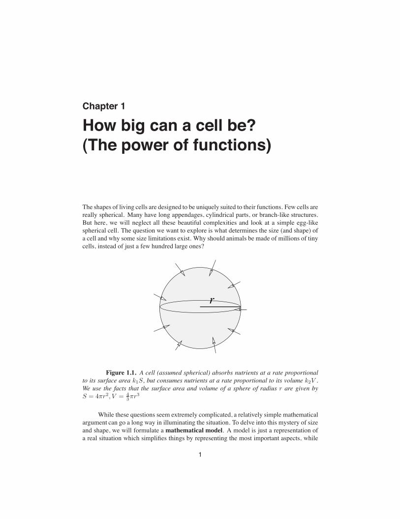
The shapes of living cells are designed to be uniquely suited to their functions. Few cells arereally spherical. Many have long appendages, cylindrical parts, or branch-like structures.But here, we will neglect all these beautiful complexities and look at a simple egg-likespherical cell. The question we want to explore is what determines the size (and shape) ofa cell and why some size limitations exist. Why should animals be made of millions of tinycells, instead of just a few hundred large ones?
r
Figure 1.1. A cell (assumed spherical) absorbs nutrients at a rate proportionalto its surface area k1S, but consumes nutrients at a rate proportional to its volume k2V .We use the facts that the surface area and volume of a sphere of radius r are given byS = 4πr2, V = 4
3πr3
While these questions seem extremely complicated, a relatively simple mathematicalargument can go a long way in illuminating the situation. To delve into this mystery of sizeand shape, we will formulate a mathematical model. A model is just a representation ofa real situation which simplifies things by representing the most important aspects, while
1
2 Chapter 1. How big can a cell be? (The power of functions)
neglecting or idealizing the other aspects. Below we follow a reasonable set of assumptionsand mathematical facts to explore how nutrient balance can affect and limit cell size.
In exploring this problem, we will encounter power functions. This will motivate adiscussion of the shapes and properties of such functions, and how they behave for smalland large values of the independent variable.
1.1 A simple model for nutrient balance in the cellWe base the model on the following assumptions:
1. The cell is roughly spherical (See Figure 1.1).
2. The cell absorbs oxygen and nutrients from the environment through its surface. Ifthe surface area, S, of the cell is bigger, it can absorb these substances at a fasterrate. We will assume that the rate at which nutrients (or oxygen) are absorbed isproportional to the surface area of the cell.
3. The rate at which nutrients are consumed in metabolism (i.e. used up) is propor-tional to the volume, V , of the cell; This means that the rate of consumption is someconstant multiple of the volume, and it also implies that the bigger the volume, themore nutrients are needed to keep the cell alive. We will assume that the rate at whichnutrients (or oxygen) are consumed is proportional to the volume of the cell.
We define the following quantities for our model of a single cell:
A = net rate of absorption of nutrients per unit time,C = net rate of consumption of nutrients per unit time,V = cell volume,S = cell surface area,r = radius of the cell.
We now rephrase the assumptions mathematically. By assumption (2), A is propor-tional to S: This means that
A = k1S,
where k1 is a constant of proportionality. Since absorption and surface area are positivequantities, in this case only positive values of the proportionality constant make sense, sothat k1 > 0. (The value of this constant would depend on the permeability of the cell mem-brane, how many pores or channels it contains, and/or any active transport mechanisms thathelp transfer substances across the cell surface into its interior.
Further, by assumption (3), C is proportional to V , so that
C = k2V,
where k2 > 0 is a second proportionality constant. The value of k2 would depend on therate of metabolism of the cell, i.e. how quickly it consumes nutrients in carrying out itsactivities.
1.2. Power functions 3
Since we have assumed that the cell is spherical, by assumption (1), the surface area,S, and volume V of the cell are:
S = 4πr2, V =4
3πr3. (1.1)
Putting these facts together leads to the following relationships between nutrient absorption,consumption, and cell radius:
A = k1(4πr2) = (4πk1)r
2, C = k2
(
4
3πr3
)
=
(
4
3πk2
)
r3.
We note that A,C are now quantities that depend on the radius of the cell. Indeed, since theterms in brackets on the right hand sides are just constant coefficients, each of the aboveexpressions is simply a power function, with r the independent variable, that is
A(r) = ar2, C(r) = cr3 (where a = 4πk1, c =4
3πk2 are constants).
Each of these expressions has the form
y = K rn
for some positive constant coefficient K Most importantly, the powers are n = 3 for con-sumption and n = 2 for absorption.
In order to appreciate how the size of the cell affects each of the two processes con-sumption and absorption of nutrients, let us review some elementary facts about powerfunctions.
1.2 Power functionsA power function has the form
y = f(x) = Kxn
where n is a positive integer and K is a constant. For simplicity, we here take K = 1.Power functions are among the most elementary and “elegant” functions. They are easy tocalculate1, are very predictable and smooth, and, from the point of view of calculus, arevery easy to handle.
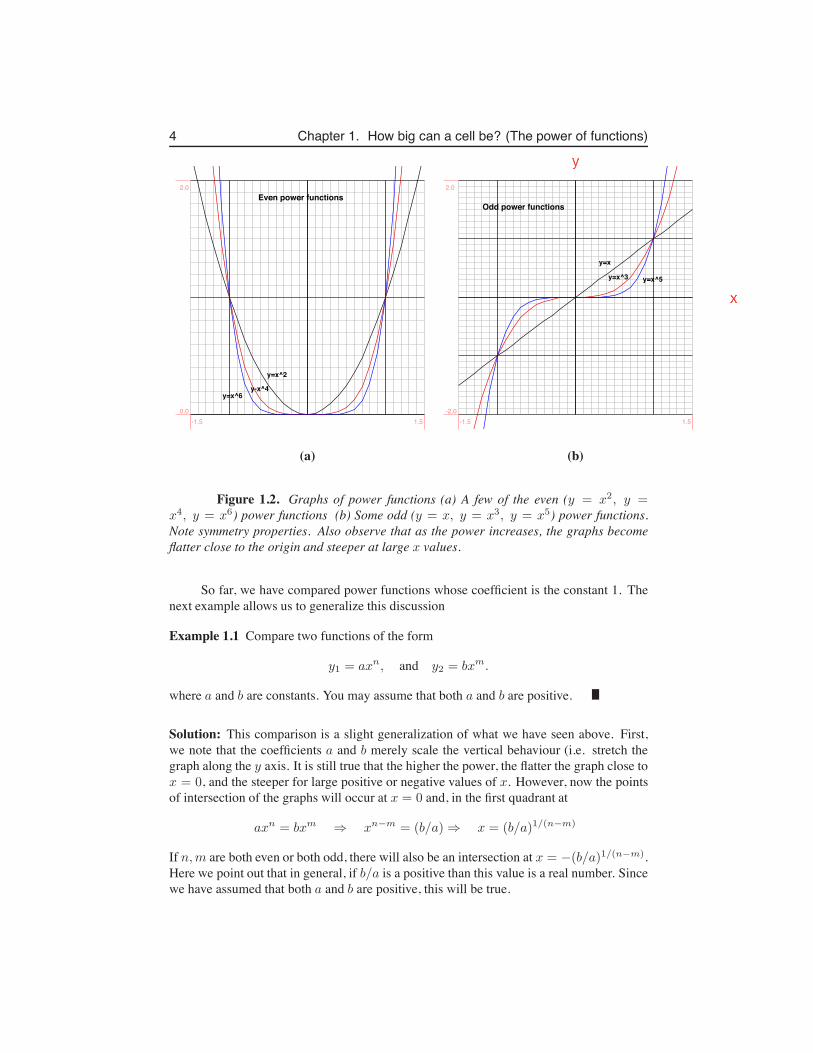
As shown in Fig. 1.2, even and odd powers lead to power functions of distinct sym-metry properties. Indeed the terms even and odd functions stem directly from the symme-try properties of the power functions. (See Appendix C for a review of symmetry.) FromFigure 1.2, we see that all the elementary power functions intersect at x = 0 and x = 1.Each of the even (odd) power functions also intersect one another at x = −1.
Figure 1.2 also demonstrates another extremely important feature of the power func-tions: the higher the power, the flatter the graph near the origin and the steeper the graphbeyond |x| > 1. This can be restated in terms of the relative size of the power functions.We say that close to the origin, the functions with lower powers dominate, while far fromthe origin, the higher powers dominate.
1We only need to use multiplication to compute the value of these functions at any point.
4 Chapter 1. How big can a cell be? (The power of functions)
Even power functions
y=x^2
y-x^4y=x^6
-1.5 1.50.0
2.0
Odd power functions
y=x
y=x^3 y=x^5
-1.5 1.5-2.0
2.0
(a) (b)
Figure 1.2. Graphs of power functions (a) A few of the even (y = x2, y =x4, y = x6) power functions (b) Some odd (y = x, y = x3, y = x5) power functions.Note symmetry properties. Also observe that as the power increases, the graphs becomeflatter close to the origin and steeper at large x values.
So far, we have compared power functions whose coefficient is the constant 1. Thenext example allows us to generalize this discussion
Example 1.1 Compare two functions of the form
y1 = axn, and y2 = bxm.
where a and b are constants. You may assume that both a and b are positive.
Solution: This comparison is a slight generalization of what we have seen above. First,we note that the coefficients a and b merely scale the vertical behaviour (i.e. stretch thegraph along the y axis. It is still true that the higher the power, the flatter the graph close tox = 0, and the steeper for large positive or negative values of x. However, now the pointsof intersection of the graphs will occur at x = 0 and, in the first quadrant at
axn = bxm ⇒ xn−m = (b/a) ⇒ x = (b/a)1/(n−m)
If n,m are both even or both odd, there will also be an intersection at x = −(b/a)1/(n−m).Here we point out that in general, if b/a is a positive than this value is a real number. Sincewe have assumed that both a and b are positive, this will be true.
Leah Keshet
x
Leah Keshet
y
1.3. Cell size for nutrient balance, continued 5
Example 1.2 Determine points of intersection for the following pairs of functions: (a)y1 = 3x4 and y2 = 27x2, (b) y1 = (4/3)πx3, y2 = 4πx2.
Solution: (a) intersections occur at x = 0 and at ±(27/3)1/(4−2) = ±√9 = ±3. (b)
These functions intersect only at x = 0, 3 but not for any negative values of x.
In many cases, the points of intersection will be irrational numbers whose decimalapproximations can only be obtained by a scientific calculator or some other method (e.g.see Newton’s Method in a later chapter).
1.3 Cell size for nutrient balance, continuedIn our discussion of cell size, we found two power functions that depend on the cell radius,namely the nutrient absorption and consumption rates,
A(r) = (4πk1)r2, and C(r) =
(
4
3πk2
)
r3.
The coefficients are indicated by terms in braces, each of which is a constant. Based on ourdiscussion of power functions, we can characterize whether absorption or consumption ofnutrients dominates for small, medium, or large cells.
Example 1.3 Discuss how the dependence of nutrient absorption and consumption on cellradius implies that one process dominates for small cells while another dominates for largecells. At what cell radius do these switch in dominance?
Solution: As discussed, for small r, the power function with the lower power of r (namelyA) dominates, but for very large values of r, the power function with the higher power (C)dominates. Where does the switch take place? As before, we find this by computing thepoint of intersection of the two graphs
A(r) = C(r) ⇒(
4
3πk2
)
r3 = (4πk1)r2.
One solution to this equation (which is not too interesting here) is r = 0. If r $= 0, then wecan cancel a factor of r2 from both sides to obtain:
r = 3k1k2
.
For cells of this radius, absorption and consumption are equal, it follows that for smaller cellsizes the absorptionA ≈ r2 is the dominant process, which for large cells, the consumptionC ≈ r3 is higher than absorption. We conclude that cells larger than the critical sizer = 3k1/k2 will be unable to keep up with the nutrient demand, and will not survive.
Thus, using this simple geometric argument, we have deduced that the size of the cellhas strong implications on its ability to absorb nutrients quickly enough to feed itself. The
6 Chapter 1. How big can a cell be? (The power of functions)
restriction on oxygen absorption is even more critical than the replenishment of other sub-stances such as glucose. For these reasons, cells larger than some maximal size (roughly 1mm in diameter) rarely occur. Furthermore, organisms that are bigger than this size cannotrely on simple diffusion to carry oxygen to their parts—they must develop a circulatorysystem to allow more rapid dispersal of such life-giving substances or else they will perish.
1.4 Observations about the “shapes” of powerfunctions
Before moving on, we collect some important observations that will prove helpful in othercontexts. Here we merely draw conclusions based on the graphs of power functions, butlater on, some of these properties will be studied in general
1.4.1 Even and odd (power) functionsFrom Fig 1.2(a) we see that power functions such as y = x2, y = x4 that have an evenpower are symmetric about the y axis, whereas from Fig 1.2(b) it is clear that odd powerfunctions such as y = x, y = x3 and so on are symmetric when rotated about the origin.We adopt the term even function and odd function to describe such symmetry properties.
More formally, if f is an even function the f(−x) = f(x), whereas if f is an oddfunction then f(−x) = −f(x). Many functions have no symmetry whatever, and areneither even nor odd. See Appendix C.D for details.
Example 1.4 Show that the function y = g(x) = x2 − 3x4 is an even function
Solution: We use the property that an even function should satisfy f(−x) = f(x). Wewrite g(−x) = (−x)2 − 3(−x)4 = x2 − 3x4 = g(x). Here we have used the fact that thequantity (−x), raised to any even power is the same as x raised to that power.
1.4.2 Maxima, minima, and behaviour “at infinity”From Fig 1.2 we see that all power functions go through the point (0, 0). Even powerfunctions have a local minimum at the origin whereas odd power functions do not.
Definition 1.5 (Local Minimum). A local minimum of a function f(x) is a point xmin
such that the value of f is larger at all sufficiently close points. Formally, f(xmin ± ε) >f(xmin) for ε small enough.
All power functions are continuous and unbounded. For x → ∞ both even and oddpower functions satisfy y = xn → ∞. For x → −∞, odd power functions tend to −∞.
1.4.3 Inverse functionsIn Examples 1.1-1.2, we used the idea that a relationship of the form y = xn can be writtenin the alternate form y1/n = x. The power function with fractional power 1/n “inverts”the operation of the integer power n. We say that

1.5. Polynomials 7
For x > 0 the function g(x) = x1/n is the inverse of the function f(x) =xn. In this case, we also use the notation g(x) = f−1(x) to denote theinverse function.
Odd power functions have the property that they are one-to-one. (That is, each valueof y is obtained from a unique value of x and vice versa.) This means that for odd powerfunctions the above relationship holds for all real x, not only for positive values. That thisis not the case for the even power functions can be seen from the example 22 = (−2)2 = 4:The function y = x2 is not one-to-one. For this reason, inverting the even power functionsis possible only if we restrict the domain to x > 0. Thus, we can associate y = x2 with theinverse x = y1/2 =
√y only for positive values of x and y.
1.5 PolynomialsA polynomial is a function in which the simple power functions are combined in a simpleway. A typical example is
y = p(x) = anxn + an−1x
n−1 + · · ·+ a1x+ a0.
This superposition of the basic power functions with integer powers and real coefficientsak proves to be a function with particularly convenient features in terms of computations:evaluating p at any point x reduces to simple arithmetical operations of multiplications andaddition (something that computers are well equipped for). Furthermore, as we shall see,these functions are easy to treat using basic calculus operations that we will describe in thefollowing chapters. The highest power n is called the degree of the polynomial.
In Appendix C, we present some of the special features of polynomials. Here we canbriefly mention that a polynomial of degree n can have up to n−1 “wiggles” (by which wemeanmaxima andminima). Every polynomial is unbounded as x → ∞ and as x → −∞.In fact, for large enough values of x, the power function y = f(x) = anxn with the largestpower, n, dominates so that
p(x) ≈ anxn for large x.
Similarly, for small x, close to the origin, the smallest powers dominates so that
p(x) ≈ a1x+ a0 for small x.
Example 1.6 Sketch the polynomial
y = p(x) = x3 + ax.
How would the sketch change if the constant a changes from positive or negative?
Solution: The polynomial has two terms, and we will consider their effects individually.Near the origin, for x ≈ 0 the term ax dominates so that, close to x = 0, the functionbehaves as
y ≈ ax.
8 Chapter 1. How big can a cell be? (The power of functions)
-5.0 5.0
-120.0
120.0 y
x
-0.5 0.5
-0.5
0.5 y
x
-2.0 2.0
-2.0
2.0 y
x
(a1) (b1) (c1)
-5.0 5.0
-120.0
120.0 y
x
-0.5 0.5
-0.5
0.5 y
x
-2.0 2.0
-2.0
2.0 y
x
(a2) (b2) (c2)
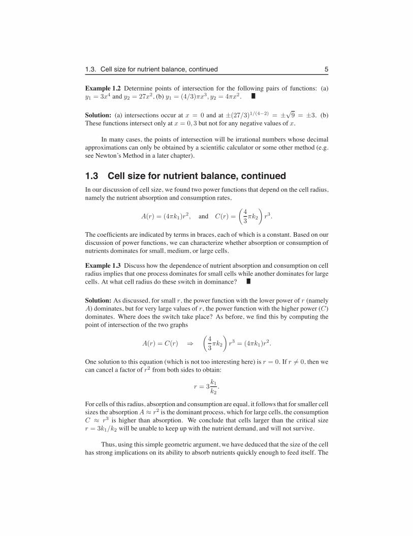
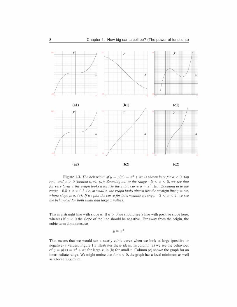
Figure 1.3. The behaviour of y = p(x) = x3 + ax is shown here for a < 0 (toprow) and a > 0 (bottom row). (a): Zooming out to the range −5 < x < 5, we see thatfor very large x the graph looks a lot like the cubic curve y = x3. (b): Zooming in to therange −0.5 < x < 0.5, i.e. at small x, the graph looks almost like the straight line y = ax,whose slope is a. (c): If we plot the curve for intermediate x range, −2 < x < 2, we seethe behaviour for both small and large x values.
This is a straight line with slope a. If a > 0 we should see a line with positive slope here,whereas if a < 0 the slope of the line should be negative. Far away from the origin, thecubic term dominates, so
y ≈ x3.
That means that we would see a nearly cubic curve when we look at large (positive ornegative) x values. Figure 1.3 illustrates these ideas. In column (a) we see the behaviourof y = p(x) = x3 + ax for large x, in (b) for small x. Column (c) shown the graph for anintermediate range. We might notice that for a < 0, the graph has a local minimum as wellas a local maximum.
1.6. Rate of an enzyme-catalyzed reaction 9
The zeros of the polynomial can be found by setting
y = p(x) = 0 ⇒ x3 + ax = 0 ⇒ x3 = −ax.
The above equation always has a solution x = 0, but if x $= 0, we can cancel and obtain
x2 = −a.
This would have no solutions if a is a positive number, so that in that case, the graphcrosses the x axis only once, at x = 0, as shown in Figure 1.3 (c2). If a is negative, thenthe negatives cancel, so the equation can be written in the form
x2 = |a|
and we would have two new zeros at
x = ±√
|a|.
For example, if a = −1 then the function y = x3 − x has zeros at x = 0, 1,−1.
1.6 Rate of an enzyme-catalyzed reactionA rational function is a function that can be written as
y =p1(x)
p2(x)where p1(x), p2(x) are polynomials.
Here we will encounter examples of such functions and their application in biochemistry.We will also find that observations about power functions will help to understand the prop-erties of such rational functions.
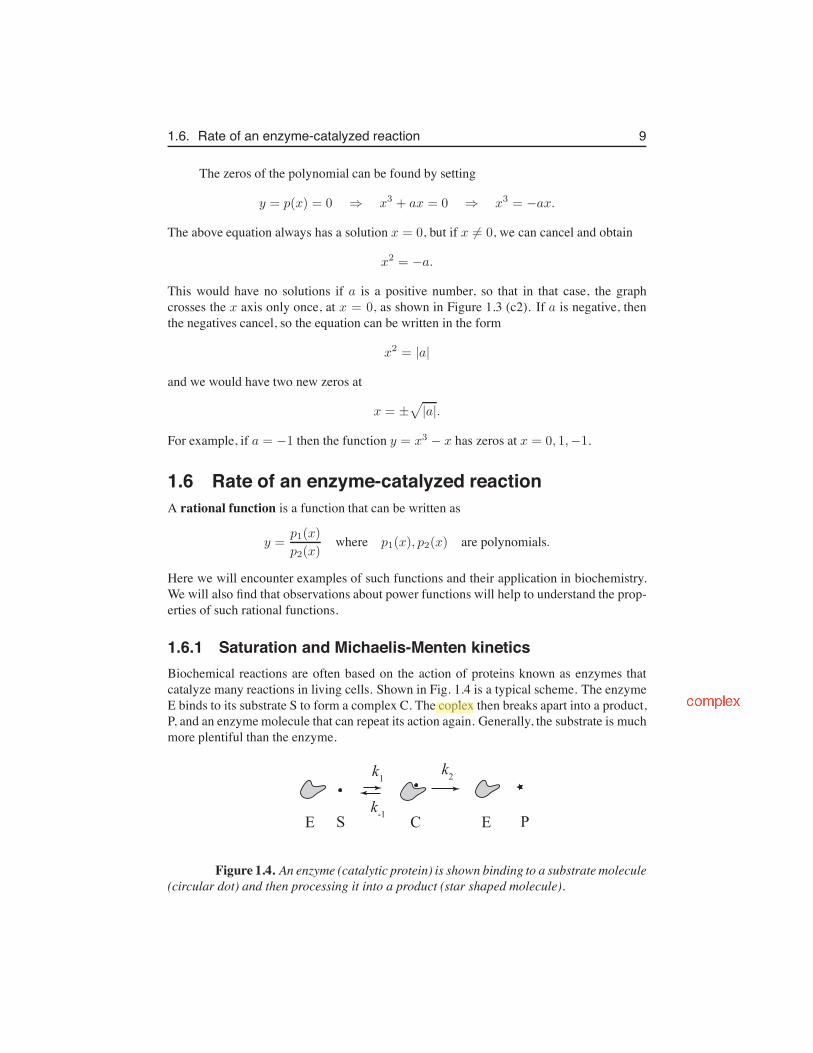
1.6.1 Saturation and Michaelis-Menten kineticsBiochemical reactions are often based on the action of proteins known as enzymes thatcatalyze many reactions in living cells. Shown in Fig. 1.4 is a typical scheme. The enzymeE binds to its substrate S to form a complex C. The coplex then breaks apart into a product,P, and an enzyme molecule that can repeat its action again. Generally, the substrate is muchmore plentiful than the enzyme.
E S C E P
k1
k-1
k2
Figure 1.4. An enzyme (catalytic protein) is shown binding to a substrate molecule(circular dot) and then processing it into a product (star shaped molecule).
Leah Keshet
Leah Keshet
complex
10 Chapter 1. How big can a cell be? (The power of functions)
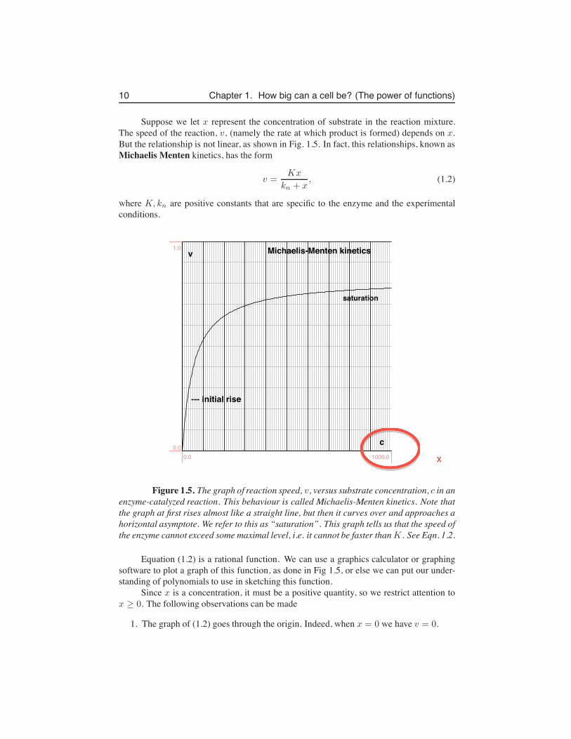
Suppose we let x represent the concentration of substrate in the reaction mixture.The speed of the reaction, v, (namely the rate at which product is formed) depends on x.But the relationship is not linear, as shown in Fig. 1.5. In fact, this relationships, known asMichaelis Menten kinetics, has the form
v =Kx
kn + x, (1.2)
where K, kn are positive constants that are specific to the enzyme and the experimentalconditions.
Michaelis-Menten kineticsv
c
--- initial rise
saturation
0.0 1000.00.0
1.0
Figure 1.5. The graph of reaction speed, v, versus substrate concentration, c in anenzyme-catalyzed reaction. This behaviour is called Michaelis-Menten kinetics. Note thatthe graph at first rises almost like a straight line, but then it curves over and approaches ahorizontal asymptote. We refer to this as “saturation”. This graph tells us that the speed ofthe enzyme cannot exceed some maximal level, i.e. it cannot be faster than K . See Eqn. 1.2.
Equation (1.2) is a rational function. We can use a graphics calculator or graphingsoftware to plot a graph of this function, as done in Fig 1.5, or else we can put our under-standing of polynomials to use in sketching this function.
Since x is a concentration, it must be a positive quantity, so we restrict attention tox ≥ 0. The following observations can be made
1. The graph of (1.2) goes through the origin. Indeed, when x = 0 we have v = 0.
Leah Keshet
Leah Keshet
x
1.6. Rate of an enzyme-catalyzed reaction 11
2. Close to the origin, the graph “looks like” a straight line. We can see this by consid-ering values of x that are much smaller than kn. Then the denominator (kn + x) iswell approximated by the constant kn. Thus, for small x, v ≈ (K/kn)x. Thus forsmall x the graph resembles a straight line with slope (K/kn).
3. For large x, there is a horizontal asymptote. The reader can use a similar argumentfor x ) kn, to show that v is approximately constant.
Michaelis-Menten kinetics thus represents one type of relationship in which the phe-nomenon of saturation occurs: the speed of the reaction increases for small increases in thelevel of substrate, but it cannot increase indefinitely, i.e. the enzymes saturate and operateat their fixed constant speed when the substrate concentration is very high.
It is worth pointing out the units of terms in (1.2). x carries units of concentration(e.g. nano Molar written nM, which means 10−9 Moles per litre) v carries units of con-centration over time (e.g. nM min−1). kn must have same units as x (only quantities withidentical units can be added or compared !). The units on the two sides of the relationship(1.2) have to balance too, meaning that K must have the same units as the speed of thereaction, v.
1.6.2 Hill functionsThe Michaelis-Menten kinetics we discussed above fit into a broader class of Hill func-tions, which are rational functions of the form
y =Axn
an + xn. (1.3)
Here A, a > 0 is a constant and n is some power. This function is often referred to as a Hillfunction with coefficient n, (although the “coefficient” is actually a power in terms of theterminology used in this chapter). Hill functions occur in biology in situations where therate of some enzyme-catalyzed reaction is affected by cooperative behaviour of a numberof subunits, or by a chain of steps.
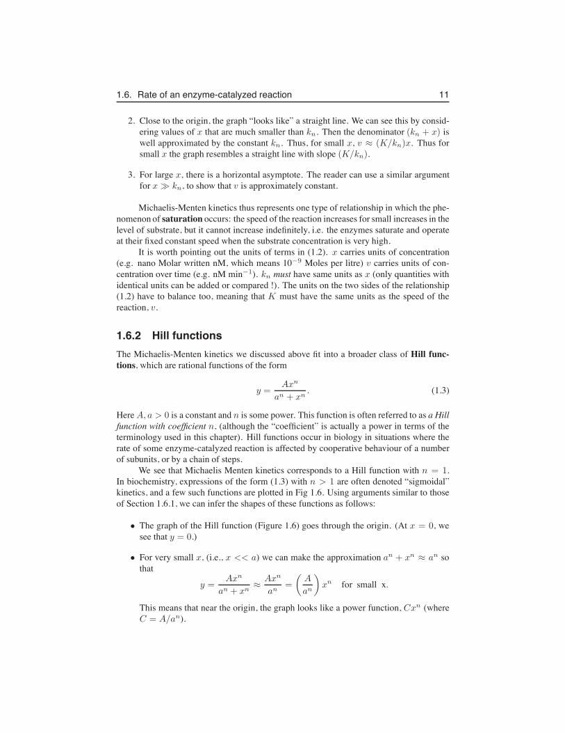
We see that Michaelis Menten kinetics corresponds to a Hill function with n = 1.In biochemistry, expressions of the form (1.3) with n > 1 are often denoted “sigmoidal”kinetics, and a few such functions are plotted in Fig 1.6. Using arguments similar to thoseof Section 1.6.1, we can infer the shapes of these functions as follows:
• The graph of the Hill function (Figure 1.6) goes through the origin. (At x = 0, wesee that y = 0.)
• For very small x, (i.e., x << a) we can make the approximation an + xn ≈ an sothat
y =Axn
an + xn≈
Axn
an=
(
A
an
)
xn for small x.
This means that near the origin, the graph looks like a power function, Cxn (whereC = A/an).

12 Chapter 1. How big can a cell be? (The power of functions)
y = 3 x^n / (1 + x^n)
n=1
n=2n=3
0.0 10.00.0
3.0
Figure 1.6. Three Hill functions with A = 3, a = 1 and coefficient n = 1, 2, 3 arecompared on this graph. As the Hill coefficient increases, the graph becomes flatter closeto the origin, and steeper in its rise to the asymptote at y = A.
• For large x, i.e. x >> a, it is approximately true that an + xn ≈ xn so that
y =Axn
an + xn≈
Axn
xn= A for large x.
This reveals that the graph has a horizontal asymptote y = A at large values of x.This means that the largest (“maximal”) value that y approaches is y = A. If yrepresents the speed of a chemical reaction (analogous to the variable we labeled vin chapter 1), then A is the “maximal rate” or “maximal speed”.
• Since the Hill function behaves like a simple power function close to the origin, weconclude directly that the higher the value of n, the flatter is its graph near 0. Further,large n means sharper rise to the eventual asymptote. Hill functions with large n areoften used to represent “switch-like” behaviour in genetic networks or biochemicalsignal transduction pathways.
• The constant a is sometimes called the “half-maximal activation level” for the fol-
1.7. For further study: Spacing of fish in a school 13
lowing reason: When x = a then
y =Aan
an + an=
Aa2
2a2=
A
2.
This shows that the level x = a leads to the half-maximal level of y.
1.7 For further study: Spacing of fish in a schoolMany animals live or function best when they are in a group. Social groups include herdsof wildebeest, flocks of birds, and schools of fish, as well as swarms of insects. Life in agroup can affect the way that individuals forage (search for food), their success at detectingor avoiding being eaten by a predator, and other functions such as mating, protection ofthe young, etc. Biologists are interested in the ecological implications of groups on theirown members or on other species with whom they interact, and how individual behaviour,combined with environmental factors and random effects affect the shape of the groups, thespacing, and the function.
In many social groups, the spacing between individuals is relatively constant fromone part of the formation to another, because animals that get too close start to move awayfrom one another, whereas those that get too far apart are attracted back. These spacingdistances can be observed in a variety of groups, and were described in many biologicalpublications. For example, Emlen [?] found that in flocks, gulls are spaced at about onebody length apart, whereas Conder [?] observed a 2-3 body lengths spacing distance intufted ducks. Miller [?] observed that sandhill cranes try to keep about 5.8 ft apart in theflock he observed.
To try to explain why certain spacing is maintained in a group of animals, it wasproposed that there are mutual attraction and repulsion interactions, (effectively acting likesimple forces) between individuals. Breder [?] followed a number of species of fish thatschool, and measured the individual spacing in units of the fish body length, showing thatindividuals are separated by 0.16-0.25 body length units. He suggested that the effectiveforces between individuals were similar to inverse power laws for repulsion and attraction.Breder considered a quantity he called cohesiveness, defined as:
c =A
xm−
R
xn, (1.4)
where A,R are magnitudes of attraction and repulsion, x is the distance between individ-uals, and m,n are integer powers that govern how quickly the interactions fall off withdistance. We could re-express (1.4) as
c = Ax−m −Rx−n
Thus, the function shown in Breder’s cohesiveness formula is related to our power func-tions, but the powers are negative integers. A specific case considered by Breder wasm = 0, n = 2, i.e. constant attraction and inverse square law repulsion,
c = A− (R/x2)
14 Chapter 1. How big can a cell be? (The power of functions)
Breder specifically considered the “point of neutrality”, where c = 0. The distance atwhich this occurs is:
x = (R/A)1/2
where attraction and repulsion are balanced. This is the distance at which two fish wouldbe most comfortable: neither tending to move apart, nor get closer together.
Other ecologists studying a similar problem have used a variety of assumptions aboutforces that cause group members to attract or repel one another.
1.8 For further study: TransformingMichaelis-Menten kinetics to a linear relationship
Michaelis-Menten kinetics that we explored in (1.2) is a nonlinear saturating function inwhich the concentration x is the independent variable on which the reaction velocity, vdepends. As discussed in Section 1.6.1, the constants K and kn depend on the enzyme andare often quantified in a biochemical assay of enzyme action. In older times, a convenientway to estimate the values of K and kn was to measure v for many different values of theinitial substrate concentration. Before nonlinear fitting software was widely available, theexpression (1.2) was transformed (meaning that it was rewritten as a linear relationship.
We can do so with the following algebraic steps:
v =Kx
kn + x
so, taking reciprocals and expanding leads to
1
v=
kn + x
Kx,
=knKx
+x
Kx
=
(
knK
)
1
x+
(
1
K
)
This suggests defining the two constants:
m =knK
, b =1
K.
In which case, the relationship between 1/v and 1/x becomes linear:[
1
v
]
= m
[
1
x
]
+ b. (1.5)
Both the slope, m and intercept b of the straight line provide information about the param-eters. The relationship (1.5), which is a disguised variant of Michaelian kinetics is calledthe Linweaver-Burke relationship. Later, we will see how this can be used to estimate thevalues of K and kn from biochemical data about an enzyme.
Exercises 15
Exercises1.1. Simple transformations: Consider the graphs of the simple functions y = x, y =
x2, and y = x3. What happens to each of these graphs when the functions aretransformed as follows:
(a) y = Ax, y = Ax2, and y = Ax3 where A > 1 is some constant.(b) y = x+ a, y = x2 + a, and y = x3 + a where a > 0 is some constant.(c) y = (x − b)2, and y = (x − b)3 where b > 0 is some constant.
1.2. Simple sketches: Sketch the graphs of the following functions:(a) y = x2,(b) y = (x + 4)2
(c) y = a(x − b)2 + c for the case a > 0, b > 0, c > 0.(d) Comment on the effects of the constants a, b, c on the properties of the graph
of y = a(x− b)2 + c.1.3. Power functions: Consider the functions y = xn, y = x1/n, y = x−n, where n is
an integer (n = 1, 2..) Which of these functions increases most steeply for values ofx greater than 1? Which decreases for large values of x? Which functions are notdefined for negative x values? Compare the values of these functions for 0 < x < 1.Which of these functions are not defined at x = 0?
1.4. Finding points of intersection(I):(a) Consider the two functions f(x) = 3x2 and g(x) = 2x5. Find all points of
intersection of these functions.(b) Repeat the calculation for the two functions f(x) = x3 and g(x) = 4x5.
1.5. Finding points of intersection(II): Consider the two functions f(x) = Axn andg(x) = Bxm. Suppose m > n > 1 are integers, and A,B > 0. Determine thevalues of x at which the values of the functions are the same. Are there two placesof intersection or three? How does this depend on the integer m − n? (Remark:The point (0,0) is always an intersection point. Thus, we are asking when there isonly one more and when there are two more intersection points. See Problem 4 fora simple example of both types.)
1.6. More intersection points: Find the intersection of each pair of functions.(a) y =
√x, y = x2
(b) y = −√x, y = x2
(c) y = x2 − 1, x2
4 + y2 = 1
1.7. Roots of a quadratic: Find the range of m such that the equation x2 − 2x−m = 0has two unequal roots.
1.8. Power functions with negative powers: Consider the function
f(x) =A
xa
16 Chapter 1. How big can a cell be? (The power of functions)
where A > 0, a > 1, with a an integer. This is the same as the function f(x) =Ax−a, which is a power function with a negative power.
(a) Sketch a rough graph of this function for x > 0.(b) How does the function change if A is increased?(c) How does the function change if a is increased?
1.9. Intersections of functions with negative powers: Consider two functions of theform
f(x) =A
xa, g(x) =
B
xb.
Suppose that A,B > 0, a, b > 1 and that A > B. Determine where these functionsintersect for positive x values.
1.10. Zeros of polynomials: Find all real zeros of the following polynomials:(a) x3 − 2x2 − 3x
(b) x5 − 1
(c) 3x2 + 5x− 2.(d) Find the points of intersection of the functions y = x3 + x2 − 2x + 1 and
y = x3.1.11. Qualitative sketching skills:
(a) Sketch the graph of the function y = ax− x5 for positive and negative valuesof the constant a. Comment on behaviour close to zero and far away fromzero.
(b) What are the zeros of this function and how does this depend on a ?(c) For what values of a would you expect that this function would have a local
maximum (“peak”) and a local minimum (“valley”)?1.12. Inverse functions: The functions y = x3 and y = x1/3 are inverse functions.
(a) Sketch both functions on the same graph for −2 < x < 2 showing clearlywhere they intersect.
(b) The tangent line to the curve y = x3 at the point (1,1) has slope m = 3,whereas the tangent line to y = x1/3 at the point (1,1) has slope m = 1/3.Explain the relationship of the two slopes.
1.13. Properties of a cube: The volume V and surface area S of a cube whose sides havelength a are given by the formulae
V = a3, S = 6a2.
Note that these relationships are expressed in terms of power functions. The inde-pendent variable is a, not x. We say that “V is a function of a” (and also “S is afunction of a”).
(a) Sketch V as a function of a and S as a function of a on the same set of axes.Which one grows faster as a increases?
Exercises 17
(b) What is the ratio of the volume to the surface area; that is, what is VS in terms
of a? Sketch a graph of VS as a function of a.
(c) The formulae above tell us the volume and the area of a cube of a given sidelength. But suppose we are given either the volume or the surface area andasked to find the side. Find the length of the side as a function of the volume(i.e. express a in terms of V ). Find the side as a function of the surface area.Use your results to find the side of a cubic tank whose volume is 1 litre (1 litre= 103 cm3). Find the side of a cubic tank whose surface area is 10 cm2.
1.14. Properties of a sphere: The volume V and surface area S of a sphere of radius rare given by the formulae
V =4π
3r3, S = 4πr2.
Note that these relationships are expressed in terms of power functions with constantmultiples such as 4π. The independent variable is r, not x. We say that “V is afunction of r” (and also “S is a function of r”).
(a) Sketch V as a function of r and S as a function of r on the same set of axes.Which one grows faster as r increases?
(b) What is the ratio of the volume to the surface area; that is, what is VS in terms
of r? Sketch a graph of VS as a function of r.
(c) The formulae above tell us the volume and the area of a sphere of a givenradius. But suppose we are given either the volume or the surface area andasked to find the radius. Find the radius as a function of the volume (i.e.express r in terms of V ). Find the radius as a function of the surface area. Useyour results to find the radius of a balloon whose volume is 1 litre. (1 litre =103 cm3). Find the radius of a balloon whose surface area is 10 cm2
1.15. The size of cell: Consider a cell in the shape of a thin cylinder (length L and ra-dius r). Assume that the cell absorbs nutrient through its surface at rate k1S andconsumes nutrients at rate k2V where S, V are the surface area and volume of thecylinder. Here we assume that k1 = 12µM µm−2 per min and k2 = 2µM µm−3
per min. (Note: µM is 10−6 moles. µm is 10−6meters.) Use the fact that a cylinder(without end-caps) has surface area S = 2πrL and volume V = πr2L to determinethe cell radius such that the rate of consumption exactly balances the rate of absorp-tion. What do you expect happens to cells with a bigger or smaller radius? Howdoes the length of the cylinder affect this nutrient balance?
1.16. Allometric relationship: Properties of animals are often related to their physicalsize or mass. For example, the metabolic rate of the animal (R), and its pulse rate(P ) may be related to its body mass m by the approximate formulae R = Amb andP = Cmd, where A,C, b, d are positive constants. Such relationships are known asallometric relationships.
(a) Use these formulae to derive a relationship between the metabolic rate and thepulse rate (Hint: eliminate m).
18 Chapter 1. How big can a cell be? (The power of functions)
(b) A similar process can be used to relate the Volume V = (4/3)πr3 and surfacearea S = 4πr2 of a sphere to one another. Eliminate r to find the correspond-ing relationship between volume and surface area for a sphere.
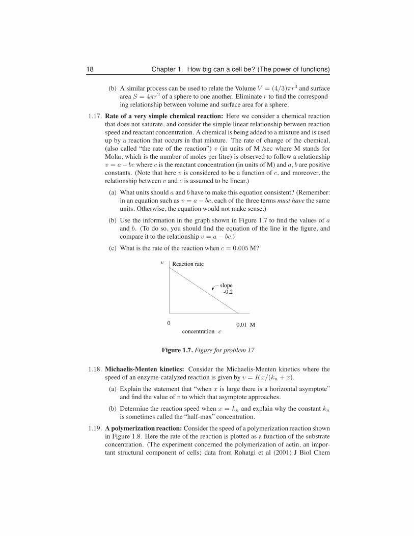
1.17. Rate of a very simple chemical reaction: Here we consider a chemical reactionthat does not saturate, and consider the simple linear relationship between reactionspeed and reactant concentration. A chemical is being added to a mixture and is usedup by a reaction that occurs in that mixture. The rate of change of the chemical,(also called “the rate of the reaction”) v (in units of M /sec where M stands forMolar, which is the number of moles per litre) is observed to follow a relationshipv = a− bc where c is the reactant concentration (in units of M) and a, b are positiveconstants. (Note that here v is considered to be a function of c, and moreover, therelationship between v and c is assumed to be linear.)
(a) What units should a and b have to make this equation consistent? (Remember:in an equation such as v = a− bc, each of the three terms must have the sameunits. Otherwise, the equation would not make sense.)
(b) Use the information in the graph shown in Figure 1.7 to find the values of aand b. (To do so, you should find the equation of the line in the figure, andcompare it to the relationship v = a− bc.)
(c) What is the rate of the reaction when c = 0.005 M?
0 0.01 Mconcentration
v
c
slope
Reaction rate
-0.2
Figure 1.7. Figure for problem 17
1.18. Michaelis-Menten kinetics: Consider the Michaelis-Menten kinetics where thespeed of an enzyme-catalyzed reaction is given by v = Kx/(kn + x).
(a) Explain the statement that “when x is large there is a horizontal asymptote”and find the value of v to which that asymptote approaches.
(b) Determine the reaction speed when x = kn and explain why the constant knis sometimes called the “half-max” concentration.
1.19. A polymerization reaction: Consider the speed of a polymerization reaction shownin Figure 1.8. Here the rate of the reaction is plotted as a function of the substrateconcentration. (The experiment concerned the polymerization of actin, an impor-tant structural component of cells; data from Rohatgi et al (2001) J Biol Chem
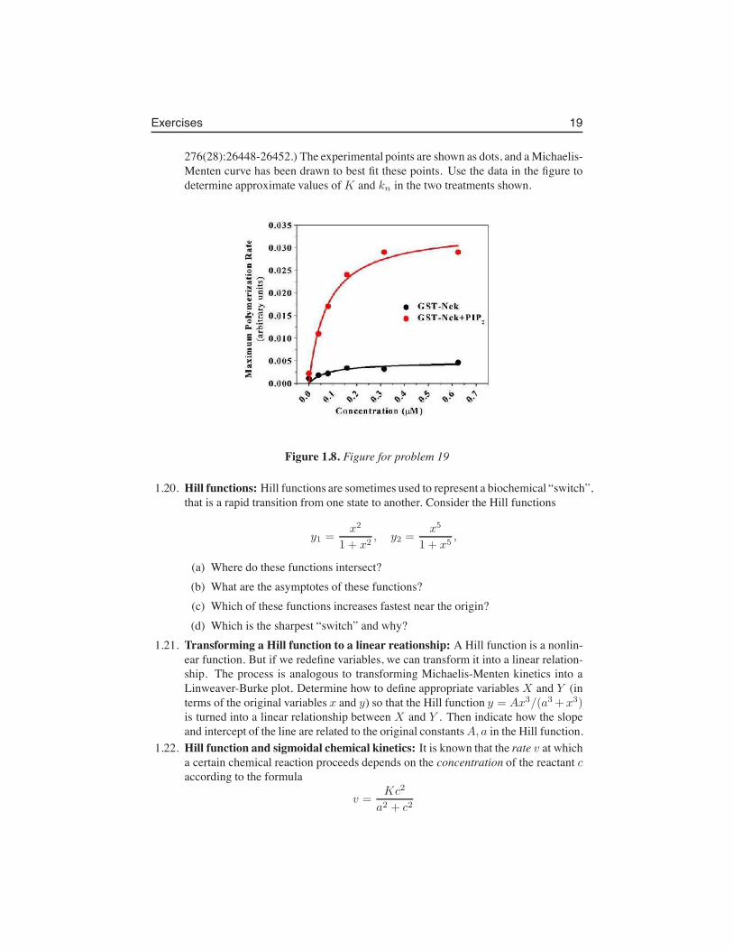
Exercises 19
276(28):26448-26452.) The experimental points are shown as dots, and a Michaelis-Menten curve has been drawn to best fit these points. Use the data in the figure todetermine approximate values of K and kn in the two treatments shown.
Figure 1.8. Figure for problem 19
1.20. Hill functions: Hill functions are sometimes used to represent a biochemical “switch”,that is a rapid transition from one state to another. Consider the Hill functions
y1 =x2
1 + x2, y2 =
x5
1 + x5,
(a) Where do these functions intersect?(b) What are the asymptotes of these functions?(c) Which of these functions increases fastest near the origin?(d) Which is the sharpest “switch” and why?
1.21. Transforming a Hill function to a linear reationship: A Hill function is a nonlin-ear function. But if we redefine variables, we can transform it into a linear relation-ship. The process is analogous to transforming Michaelis-Menten kinetics into aLinweaver-Burke plot. Determine how to define appropriate variables X and Y (interms of the original variables x and y) so that the Hill function y = Ax3/(a3+x3)is turned into a linear relationship between X and Y . Then indicate how the slopeand intercept of the line are related to the original constants A, a in the Hill function.
1.22. Hill function and sigmoidal chemical kinetics: It is known that the rate v at whicha certain chemical reaction proceeds depends on the concentration of the reactant caccording to the formula
v =Kc2
a2 + c2
20 Chapter 1. How big can a cell be? (The power of functions)
where K , a are some constants. When the chemist plots the values of the quantity1/v (on the “y” axis) versus the values of 1/c2 (on the “x axis”), she finds that thepoints are best described by a straight line with y-intercept 2 and slope 8. Use thisresult to find the values of the constants K and a.
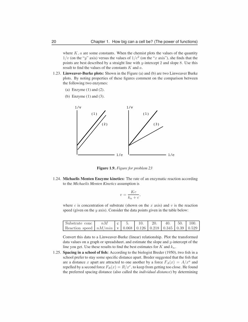
1.23. Linweaver-Burke plots: Shown in the Figure (a) and (b) are two Linweaver Burkeplots. By noting properties of these figures comment on the comparison betweenthe following two enzymes:
(a) Enzyme (1) and (2).(b) Enzyme (1) and (3).
(1)
(2)
1/c
1/v
(1)
(3)
1/c
1/v
Figure 1.9. Figure for problem 23
1.24. Michaelis Menten Enzyme kinetics: The rate of an enzymatic reaction accordingto the Michaelis Menten Kinetics assumption is
v =Kc
kn + c,
where c is concentration of substrate (shown on the x axis) and v is the reactionspeed (given on the y axis). Consider the data points given in the table below:
Substrate conc nM c 5. 10. 20. 40. 50. 100.Reaction speed nM/min v 0.068 0.126 0.218 0.345 0.39 0.529
Convert this data to a Linweaver-Burke (linear) relationship. Plot the transformeddata values on a graph or spreadsheet, and estimate the slope and y-intercept of theline you get. Use these results to find the best estimates for K and kn.
1.25. Spacing in a school of fish: According to the biologist Breder (1950), two fish in aschool prefer to stay some specific distance apart. Breder suggested that the fish thatare a distance x apart are attracted to one another by a force FA(x) = A/xa andrepelled by a second force FR(x) = R/xr, to keep from getting too close. He foundthe preferred spacing distance (also called the individual distance) by determining
Exercises 21
the value of x at which the repulsion and the attraction exactly balance. Find theindividual distance in terms of the quantities A,R, a, r (all assumed to be positiveconstants.)

22 Chapter 1. How big can a cell be? (The power of functions)
Chapter 2
Average rates of change,average velocity and thesecant line
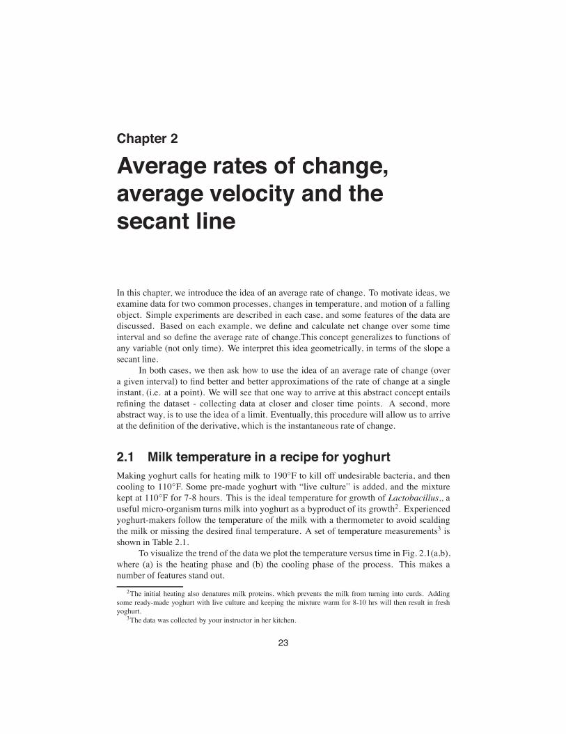
In this chapter, we introduce the idea of an average rate of change. To motivate ideas, weexamine data for two common processes, changes in temperature, and motion of a fallingobject. Simple experiments are described in each case, and some features of the data arediscussed. Based on each example, we define and calculate net change over some timeinterval and so define the average rate of change.This concept generalizes to functions ofany variable (not only time). We interpret this idea geometrically, in terms of the slope asecant line.
In both cases, we then ask how to use the idea of an average rate of change (overa given interval) to find better and better approximations of the rate of change at a singleinstant, (i.e. at a point). We will see that one way to arrive at this abstract concept entailsrefining the dataset - collecting data at closer and closer time points. A second, moreabstract way, is to use the idea of a limit. Eventually, this procedure will allow us to arriveat the definition of the derivative, which is the instantaneous rate of change.
2.1 Milk temperature in a recipe for yoghurtMaking yoghurt calls for heating milk to 190◦F to kill off undesirable bacteria, and thencooling to 110◦F. Some pre-made yoghurt with “live culture” is added, and the mixturekept at 110◦F for 7-8 hours. This is the ideal temperature for growth of Lactobacillus,, auseful micro-organism turns milk into yoghurt as a byproduct of its growth2. Experiencedyoghurt-makers follow the temperature of the milk with a thermometer to avoid scaldingthe milk or missing the desired final temperature. A set of temperature measurements3 isshown in Table 2.1.
To visualize the trend of the data we plot the temperature versus time in Fig. 2.1(a,b),where (a) is the heating phase and (b) the cooling phase of the process. This makes anumber of features stand out.
2The initial heating also denatures milk proteins, which prevents the milk from turning into curds. Addingsome ready-made yoghurt with live culture and keeping the mixture warm for 8-10 hrs will then result in freshyoghurt.
3The data was collected by your instructor in her kitchen.
23
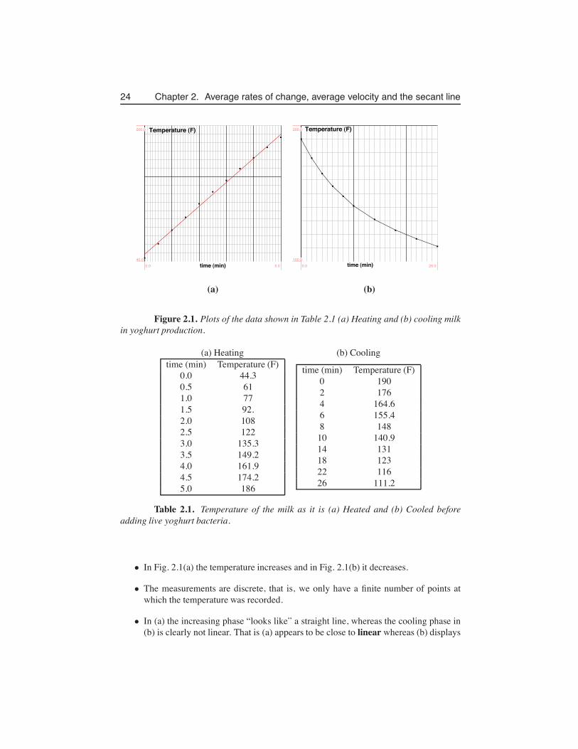
24 Chapter 2. Average rates of change, average velocity and the secant line
Temperature (F)
time (min)0.0 5.040.0
200.0 Temperature (F)
time (min)0.0 26.0100.0
200.0
(a) (b)
Figure 2.1. Plots of the data shown in Table 2.1 (a) Heating and (b) cooling milkin yoghurt production.
(a) Heating (b) Coolingtime (min) Temperature (F)
0.0 44.30.5 611.0 771.5 92.2.0 1082.5 1223.0 135.33.5 149.24.0 161.94.5 174.25.0 186
time (min) Temperature (F)0 1902 1764 164.66 155.48 148
10 140.914 13118 12322 11626 111.2
Table 2.1. Temperature of the milk as it is (a) Heated and (b) Cooled beforeadding live yoghurt bacteria.
• In Fig. 2.1(a) the temperature increases and in Fig. 2.1(b) it decreases.
• The measurements are discrete, that is, we only have a finite number of points atwhich the temperature was recorded.
• In (a) the increasing phase “looks like” a straight line, whereas the cooling phase in(b) is clearly not linear. That is (a) appears to be close to linear whereas (b) displays
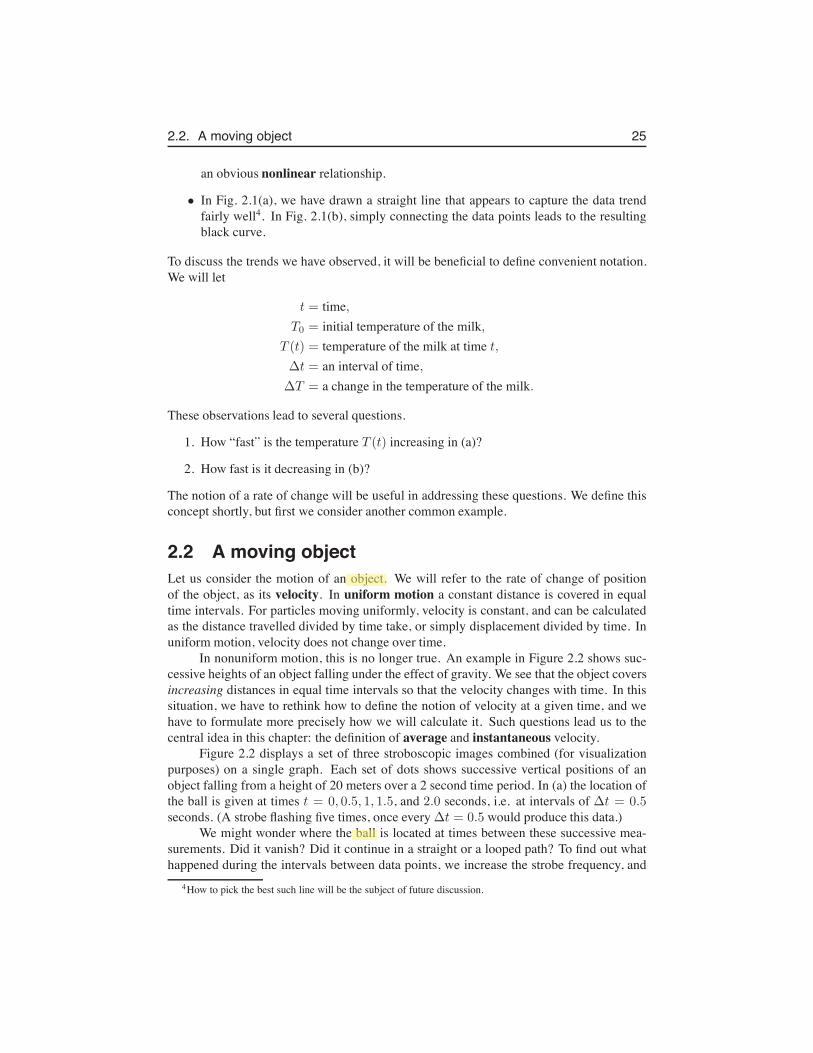
2.2. A moving object 25
an obvious nonlinear relationship.
• In Fig. 2.1(a), we have drawn a straight line that appears to capture the data trendfairly well4. In Fig. 2.1(b), simply connecting the data points leads to the resultingblack curve.
To discuss the trends we have observed, it will be beneficial to define convenient notation.We will let
t = time,T0 = initial temperature of the milk,
T (t) = temperature of the milk at time t,∆t = an interval of time,∆T = a change in the temperature of the milk.
These observations lead to several questions.
1. How “fast” is the temperature T (t) increasing in (a)?
2. How fast is it decreasing in (b)?
The notion of a rate of change will be useful in addressing these questions. We define thisconcept shortly, but first we consider another common example.
2.2 A moving objectLet us consider the motion of an object. We will refer to the rate of change of positionof the object, as its velocity. In uniform motion a constant distance is covered in equaltime intervals. For particles moving uniformly, velocity is constant, and can be calculatedas the distance travelled divided by time take, or simply displacement divided by time. Inuniform motion, velocity does not change over time.
In nonuniform motion, this is no longer true. An example in Figure 2.2 shows suc-cessive heights of an object falling under the effect of gravity. We see that the object coversincreasing distances in equal time intervals so that the velocity changes with time. In thissituation, we have to rethink how to define the notion of velocity at a given time, and wehave to formulate more precisely how we will calculate it. Such questions lead us to thecentral idea in this chapter: the definition of average and instantaneous velocity.
Figure 2.2 displays a set of three stroboscopic images combined (for visualizationpurposes) on a single graph. Each set of dots shows successive vertical positions of anobject falling from a height of 20 meters over a 2 second time period. In (a) the location ofthe ball is given at times t = 0, 0.5, 1, 1.5, and 2.0 seconds, i.e. at intervals of ∆t = 0.5seconds. (A strobe flashing five times, once every ∆t = 0.5 would produce this data.)
We might wonder where the ball is located at times between these successive mea-surements. Did it vanish? Did it continue in a straight or a looped path? To find out whathappened during the intervals between data points, we increase the strobe frequency, and
4How to pick the best such line will be the subject of future discussion.
Leah Keshet
Leah Keshet
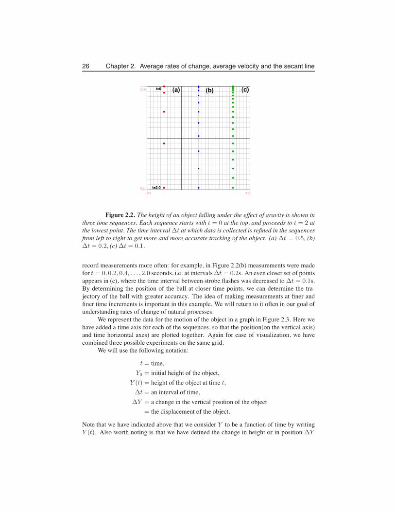
26 Chapter 2. Average rates of change, average velocity and the secant line
t=0
t=2.0
(a) (b) (c)
0.0 3.00.0
20.0
Figure 2.2. The height of an object falling under the effect of gravity is shown inthree time sequences. Each sequence starts with t = 0 at the top, and proceeds to t = 2 atthe lowest point. The time interval ∆t at which data is collected is refined in the sequencesfrom left to right to get more and more accurate tracking of the object. (a) ∆t = 0.5, (b)∆t = 0.2, (c) ∆t = 0.1.
record measurements more often: for example, in Figure 2.2(b) measurements were madefor t = 0, 0.2, 0.4, . . . , 2.0 seconds, i.e. at intervals ∆t = 0.2s. An even closer set of pointsappears in (c), where the time interval between strobe flashes was decreased to ∆t = 0.1s.By determining the position of the ball at closer time points, we can determine the tra-jectory of the ball with greater accuracy. The idea of making measurements at finer andfiner time increments is important in this example. We will return to it often in our goal ofunderstanding rates of change of natural processes.
We represent the data for the motion of the object in a graph in Figure 2.3. Here wehave added a time axis for each of the sequences, so that the position(on the vertical axis)and time horizontal axes) are plotted together. Again for ease of visualization, we havecombined three possible experiments on the same grid.
We will use the following notation:
t = time,Y0 = initial height of the object,
Y (t) = height of the object at time t,∆t = an interval of time,∆Y = a change in the vertical position of the object
= the displacement of the object.
Note that we have indicated above that we consider Y to be a function of time by writingY (t). Also worth noting is that we have defined the change in height or in position ∆Y
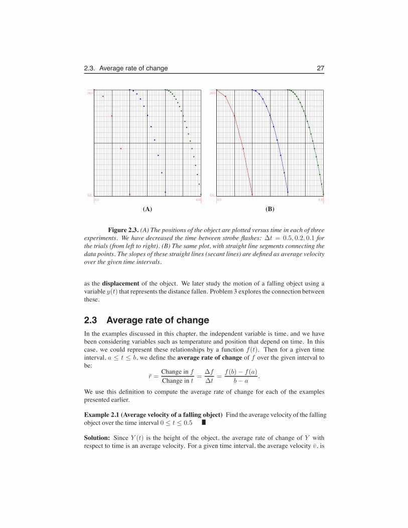
2.3. Average rate of change 27
0.0 6.00.0
20.0
0.0 6.00.0
20.0
(A) (B)
Figure 2.3. (A) The positions of the object are plotted versus time in each of threeexperiments. We have decreased the time between strobe flashes: ∆t = 0.5, 0.2, 0.1 forthe trials (from left to right). (B) The same plot, with straight line segments connecting thedata points. The slopes of these straight lines (secant lines) are defined as average velocityover the given time intervals.
as the displacement of the object. We later study the motion of a falling object using avariable y(t) that represents the distance fallen. Problem 3 explores the connection betweenthese.
2.3 Average rate of changeIn the examples discussed in this chapter, the independent variable is time, and we havebeen considering variables such as temperature and position that depend on time. In thiscase, we could represent these relationships by a function f(t). Then for a given timeinterval, a ≤ t ≤ b, we define the average rate of change of f over the given interval tobe:
r̄ =Change in f
Change in t=
∆f
∆t=
f(b)− f(a)
b− a.
We use this definition to compute the average rate of change for each of the examplespresented earlier.
Example 2.1 (Average velocity of a falling object) Find the average velocity of the fallingobject over the time interval 0 ≤ t ≤ 0.5
Solution: Since Y (t) is the height of the object, the average rate of change of Y withrespect to time is an average velocity. For a given time interval, the average velocity v̄, is
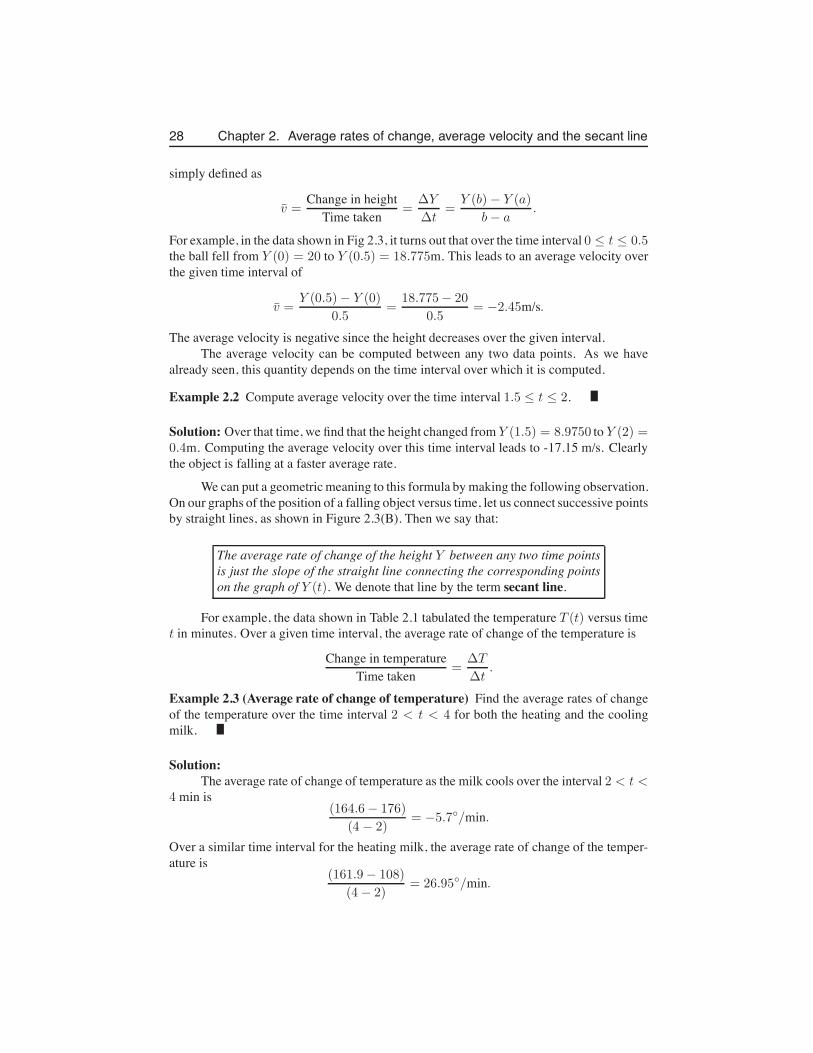
28 Chapter 2. Average rates of change, average velocity and the secant line
simply defined as
v̄ =Change in height
Time taken=
∆Y
∆t=
Y (b)− Y (a)
b− a.
For example, in the data shown in Fig 2.3, it turns out that over the time interval 0 ≤ t ≤ 0.5the ball fell from Y (0) = 20 to Y (0.5) = 18.775m. This leads to an average velocity overthe given time interval of
v̄ =Y (0.5)− Y (0)
0.5=
18.775− 20
0.5= −2.45m/s.
The average velocity is negative since the height decreases over the given interval.The average velocity can be computed between any two data points. As we have
already seen, this quantity depends on the time interval over which it is computed.
Example 2.2 Compute average velocity over the time interval 1.5 ≤ t ≤ 2.
Solution: Over that time, we find that the height changed from Y (1.5) = 8.9750 to Y (2) =0.4m. Computing the average velocity over this time interval leads to -17.15 m/s. Clearlythe object is falling at a faster average rate.
We can put a geometric meaning to this formula by making the following observation.On our graphs of the position of a falling object versus time, let us connect successive pointsby straight lines, as shown in Figure 2.3(B). Then we say that:
The average rate of change of the height Y between any two time pointsis just the slope of the straight line connecting the corresponding pointson the graph of Y (t). We denote that line by the term secant line.
For example, the data shown in Table 2.1 tabulated the temperature T (t) versus timet in minutes. Over a given time interval, the average rate of change of the temperature is
Change in temperatureTime taken
=∆T
∆t.
Example 2.3 (Average rate of change of temperature) Find the average rates of changeof the temperature over the time interval 2 < t < 4 for both the heating and the coolingmilk.
Solution:The average rate of change of temperature as the milk cools over the interval 2 < t <
4 min is(164.6− 176)
(4 − 2)= −5.7◦/min.
Over a similar time interval for the heating milk, the average rate of change of the temper-ature is
(161.9− 108)
(4− 2)= 26.95◦/min.
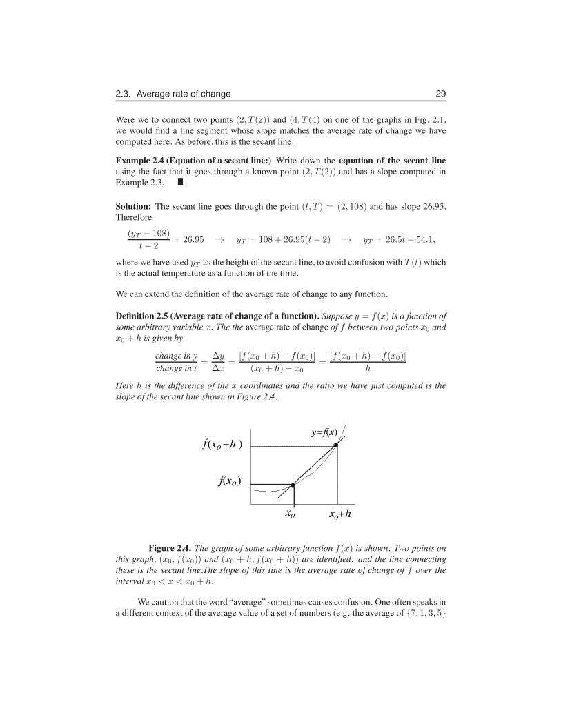
2.3. Average rate of change 29
Were we to connect two points (2, T (2)) and (4, T (4) on one of the graphs in Fig. 2.1,we would find a line segment whose slope matches the average rate of change we havecomputed here. As before, this is the secant line.
Example 2.4 (Equation of a secant line:) Write down the equation of the secant lineusing the fact that it goes through a known point (2, T (2)) and has a slope computed inExample 2.3.
Solution: The secant line goes through the point (t, T ) = (2, 108) and has slope 26.95.Therefore
(yT − 108)
t− 2= 26.95 ⇒ yT = 108 + 26.95(t− 2) ⇒ yT = 26.5t+ 54.1,
where we have used yT as the height of the secant line, to avoid confusion with T (t) whichis the actual temperature as a function of the time.
We can extend the definition of the average rate of change to any function.
Definition 2.5 (Average rate of change of a function). Suppose y = f(x) is a function ofsome arbitrary variable x. The the average rate of change of f between two points x0 andx0 + h is given by
change in ychange in t
=∆y
∆x=
[f(x0 + h)− f(x0)]
(x0 + h)− x0=
[f(x0 + h)− f(x0)]
h
Here h is the difference of the x coordinates and the ratio we have just computed is theslope of the secant line shown in Figure 2.4.
of(x +h )
x +hx oo
f(x )o
y=f(x)
Figure 2.4. The graph of some arbitrary function f(x) is shown. Two points onthis graph, (x0, f(x0)) and (x0 + h, f(x0 + h)) are identified. and the line connectingthese is the secant line.The slope of this line is the average rate of change of f over theinterval x0 < x < x0 + h.
We caution that the word “average” sometimes causes confusion. One often speaks ina different context of the average value of a set of numbers (e.g. the average of {7, 1, 3, 5}
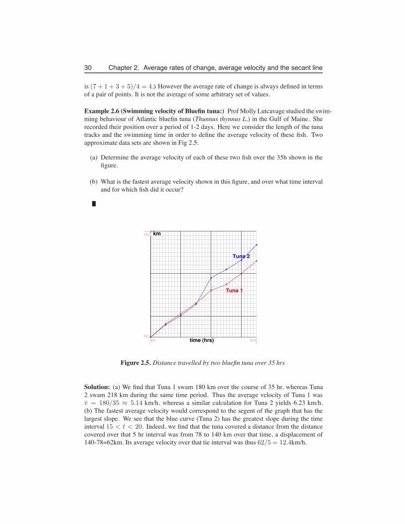
30 Chapter 2. Average rates of change, average velocity and the secant line
is (7 + 1 + 3 + 5)/4 = 4.) However the average rate of change is always defined in termsof a pair of points. It is not the average of some arbitrary set of values.
Example 2.6 (Swimming velocity of Bluefin tuna:) Prof Molly Lutcavage studied the swim-ming behaviour of Atlantic bluefin tuna (Thunnus thynnus L.) in the Gulf of Maine. Sherecorded their position over a period of 1-2 days. Here we consider the length of the tunatracks and the swimming time in order to define the average velocity of these fish. Twoapproximate data sets are shown in Fig 2.5.
(a) Determine the average velocity of each of these two fish over the 35h shown in thefigure.
(b) What is the fastest average velocity shown in this figure, and over what time intervaland for which fish did it occur?
km
time (hrs)
Tuna 1
Tuna 2
0.0 35.00.0
250.0
Figure 2.5. Distance travelled by two bluefin tuna over 35 hrs
Solution: (a) We find that Tuna 1 swam 180 km over the course of 35 hr, whereas Tuna2 swam 218 km during the same time period. Thus the average velocity of Tuna 1 wasv̄ = 180/35 ≈ 5.14 km/h, whereas a similar calculation for Tuna 2 yields 6.23 km/h.(b) The fastest average velocity would correspond to the segent of the graph that has thelargest slope. We see that the blue curve (Tuna 2) has the greatest slope during the timeinterval 15 < t < 20. Indeed, we find that the tuna covered a distance from the distancecovered over that 5 hr interval was from 78 to 140 km over that time, a displacement of140-78=62km. Its average velocity over that tie interval was thus 62/5 = 12.4km/h.
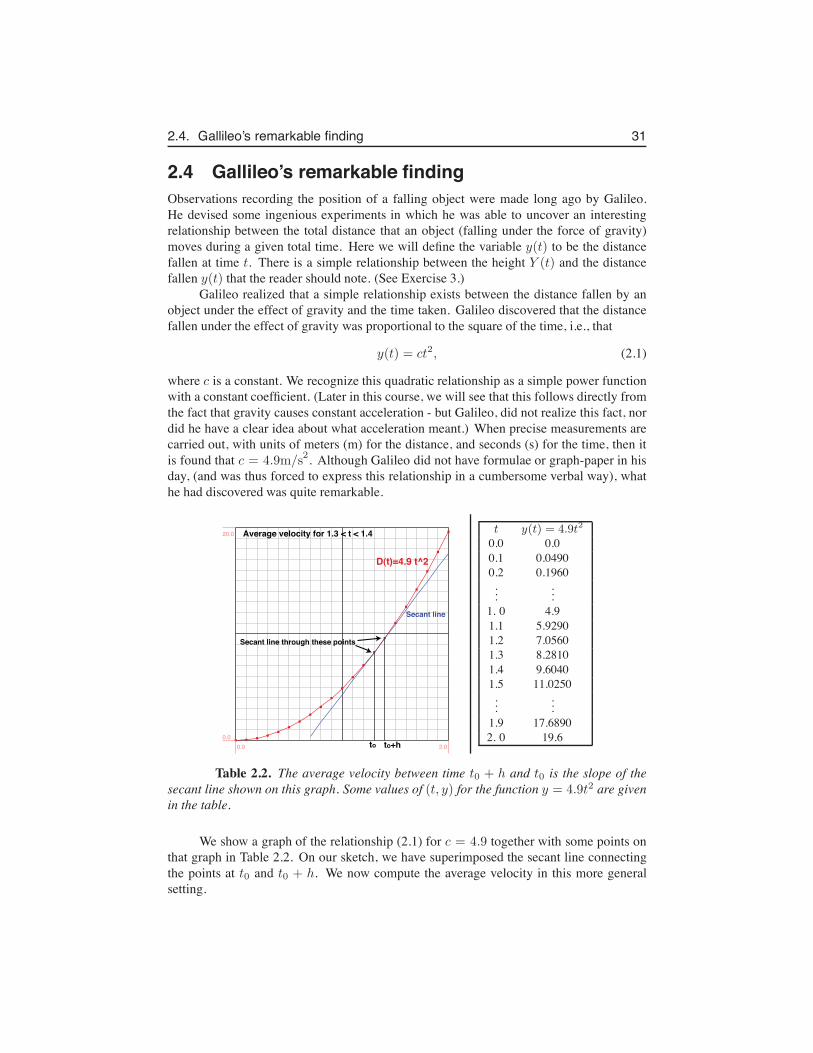
2.4. Gallileo’s remarkable finding 31
2.4 Gallileo’s remarkable findingObservations recording the position of a falling object were made long ago by Galileo.He devised some ingenious experiments in which he was able to uncover an interestingrelationship between the total distance that an object (falling under the force of gravity)moves during a given total time. Here we will define the variable y(t) to be the distancefallen at time t. There is a simple relationship between the height Y (t) and the distancefallen y(t) that the reader should note. (See Exercise 3.)
Galileo realized that a simple relationship exists between the distance fallen by anobject under the effect of gravity and the time taken. Galileo discovered that the distancefallen under the effect of gravity was proportional to the square of the time, i.e., that
y(t) = ct2, (2.1)
where c is a constant. We recognize this quadratic relationship as a simple power functionwith a constant coefficient. (Later in this course, we will see that this follows directly fromthe fact that gravity causes constant acceleration - but Galileo, did not realize this fact, nordid he have a clear idea about what acceleration meant.) When precise measurements arecarried out, with units of meters (m) for the distance, and seconds (s) for the time, then itis found that c = 4.9m/s2. Although Galileo did not have formulae or graph-paper in hisday, (and was thus forced to express this relationship in a cumbersome verbal way), whathe had discovered was quite remarkable.
to to+h
D(t)=4.9 t^2
Secant line
Secant line through these points
Average velocity for 1.3 < t < 1.4
0.0 2.0
0.0
20.0t y(t) = 4.9t2
0.0 0.00.1 0.04900.2 0.1960...
...1. 0 4.91.1 5.92901.2 7.05601.3 8.28101.4 9.60401.5 11.0250...
...1.9 17.68902. 0 19.6
Table 2.2. The average velocity between time t0 + h and t0 is the slope of thesecant line shown on this graph. Some values of (t, y) for the function y = 4.9t2 are givenin the table.
We show a graph of the relationship (2.1) for c = 4.9 together with some points onthat graph in Table 2.2. On our sketch, we have superimposed the secant line connectingthe points at t0 and t0 + h. We now compute the average velocity in this more generalsetting.
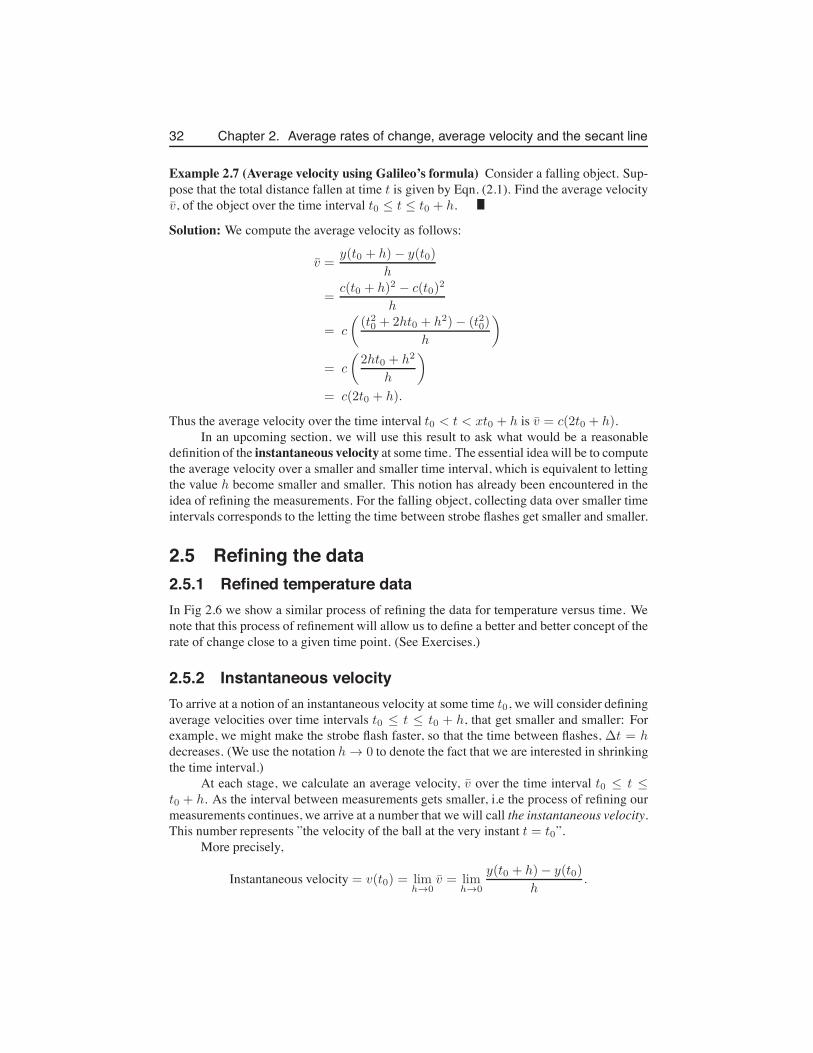
32 Chapter 2. Average rates of change, average velocity and the secant line
Example 2.7 (Average velocity using Galileo’s formula) Consider a falling object. Sup-pose that the total distance fallen at time t is given by Eqn. (2.1). Find the average velocityv̄, of the object over the time interval t0 ≤ t ≤ t0 + h.
Solution: We compute the average velocity as follows:
v̄ =y(t0 + h)− y(t0)
h
=c(t0 + h)2 − c(t0)2
h
= c
(
(t20 + 2ht0 + h2)− (t20)
h
)
= c
(
2ht0 + h2
h
)
= c(2t0 + h).
Thus the average velocity over the time interval t0 < t < xt0 + h is v̄ = c(2t0 + h).In an upcoming section, we will use this result to ask what would be a reasonable
definition of the instantaneous velocity at some time. The essential idea will be to computethe average velocity over a smaller and smaller time interval, which is equivalent to lettingthe value h become smaller and smaller. This notion has already been encountered in theidea of refining the measurements. For the falling object, collecting data over smaller timeintervals corresponds to the letting the time between strobe flashes get smaller and smaller.
2.5 Refining the data2.5.1 Refined temperature dataIn Fig 2.6 we show a similar process of refining the data for temperature versus time. Wenote that this process of refinement will allow us to define a better and better concept of therate of change close to a given time point. (See Exercises.)
2.5.2 Instantaneous velocityTo arrive at a notion of an instantaneous velocity at some time t0, we will consider definingaverage velocities over time intervals t0 ≤ t ≤ t0 + h, that get smaller and smaller: Forexample, we might make the strobe flash faster, so that the time between flashes, ∆t = hdecreases. (We use the notation h → 0 to denote the fact that we are interested in shrinkingthe time interval.)
At each stage, we calculate an average velocity, v̄ over the time interval t0 ≤ t ≤t0 + h. As the interval between measurements gets smaller, i.e the process of refining ourmeasurements continues, we arrive at a number that we will call the instantaneous velocity.This number represents ”the velocity of the ball at the very instant t = t0”.
More precisely,
Instantaneous velocity = v(t0) = limh→0
v̄ = limh→0
y(t0 + h)− y(t0)
h.
2.5. Refining the data 33
Temperature (F)
time (min)0.0 26.0100.0
200.0 Temperature (F)
time (min)0.0 26.0100.0
200.0 Temperature (F)
time (min)0.0 26.0100.0
200.0
(a) (b) (c)
Figure 2.6. Three graphs of the temperature of cooling milk showing (a) a coarsedata set (measurements every ∆t = 2 min.), (b) a more refined data set, (measurementsevery ∆t = 1 min) (c) an even more refined dataset (measurements every ∆t = 0.5 min.)
Example 2.8 Find the instantaneous velocity of the same falling object at time t0.
Solution: According to our definition, we must determine
v(t0) = limh→0
y(t0 + h)− y(t0)
h.
Our calculation would be nearly identical for v(t0) as for v̄, but for a final step of takingthe limit as h, the interval between time-points shrinks to zero:
v(t0) = limh→0
y(t0 + h)− y(t0)
h
= limh→0
c(t0 + h)2 − c(t0)2
h
= limh→0
c
(
(t20 + 2ht0 + h2)− (t20)
h
)
= limh→0
c
(
2ht0 + h2
h
)
= limh→0
c(2t0 + h)
= c(2t0) = 2ct0.
(2.2)
Remarks: In our final steps, we have allowed h to shrink. In the limit, and h → 0, weobtain the instantaneous velocity, i.e. v(t0) = 2ct0.
34 Chapter 2. Average rates of change, average velocity and the secant line
2.6 Introduction to the derivativeWith the concepts introduced in this chapter, we are ready for the the definition of thederivative.
Definition 2.9. The derivative of a function y = f(x) at a point x0 is denoted dy/dx orf ′(x0) and defined as
dy
dx= f ′(x0) = lim
h→0
[f(x0 + h)− f(x0)]
h.
Example 2.10 (Calculating the derivative) Compute the derivative of the function f(x) =Cx2 at some point x = x0.
Solution: In the previous section, we used the function y = f(t) = ct2 to calculate aninstantaneous velocity. We now recognize that our result in that problem, namely 2ct0 isthe same as the derivative of the function evaluated at t0. Thus, in a sense, we have alreadysolved this problem. By switching notation (t0 → x0 and c → C) we can write downthe answer, 2cx0 at once. However, as practice, we can rewrite the steps in the case of thegeneral point x
For y = f(x) = Cx2 we have
dy
dx= lim
h→0
f(x+ h)− f(x)
h
= limh→0
C(x + h)2 − Cx2
h
= limh→0
C(x2 + 2xh+ h2)− x2
h
= limh→0
C(2xh+ h2)
h= lim
h→0C(2x+ h)
= C(2x) = 2Cx.
Evaluating this result for x = x0 we obtain the answer 2Cx0.
We recognize from this definition that the derivative is obtained by starting with theslope of a secant line (average rate of change of f over the interval x0 < x < x0 + h)and proceeds to shrink the interval (limh→0) so that it approaches a single point (x0). Theresultant line will be denoted the tangent line. , and the value obtained will be identifiedas the the instantaneous rate of change of the function with respect to the variable x atthe point of interest, x0. Another notation used for the derivative is
df
dx
∣
∣
∣
∣
x0
.
We will explore properties and meanings of this concept in the next chapter.
Leah Keshet
Leah Keshet
typo: should be(dy/dx)|_x_0=
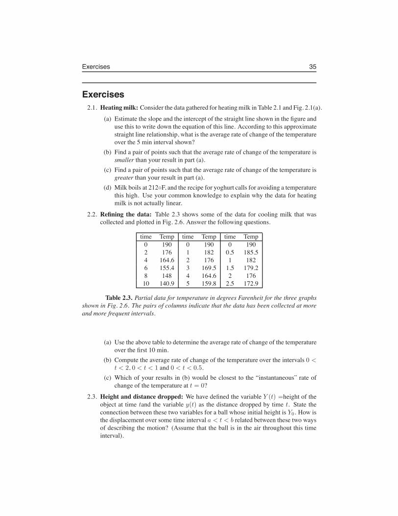
Exercises 35
Exercises2.1. Heatingmilk: Consider the data gathered for heating milk in Table 2.1 and Fig. 2.1(a).
(a) Estimate the slope and the intercept of the straight line shown in the figure anduse this to write down the equation of this line. According to this approximatestraight line relationship, what is the average rate of change of the temperatureover the 5 min interval shown?
(b) Find a pair of points such that the average rate of change of the temperature issmaller than your result in part (a).
(c) Find a pair of points such that the average rate of change of the temperature isgreater than your result in part (a).
(d) Milk boils at 212◦F, and the recipe for yoghurt calls for avoiding a temperaturethis high. Use your common knowledge to explain why the data for heatingmilk is not actually linear.
2.2. Refining the data: Table 2.3 shows some of the data for cooling milk that wascollected and plotted in Fig. 2.6. Answer the following questions.
time Temp time Temp time Temp0 190 0 190 0 1902 176 1 182 0.5 185.54 164.6 2 176 1 1826 155.4 3 169.5 1.5 179.28 148 4 164.6 2 17610 140.9 5 159.8 2.5 172.9
Table 2.3. Partial data for temperature in degrees Farenheit for the three graphsshown in Fig. 2.6. The pairs of columns indicate that the data has been collected at moreand more frequent intervals.
(a) Use the above table to determine the average rate of change of the temperatureover the first 10 min.
(b) Compute the average rate of change of the temperature over the intervals 0 <t < 2, 0 < t < 1 and 0 < t < 0.5.
(c) Which of your results in (b) would be closest to the “instantaneous” rate ofchange of the temperature at t = 0?
2.3. Height and distance dropped: We have defined the variable Y (t) =height of theobject at time tand the variable y(t) as the distance dropped by time t. State theconnection between these two variables for a ball whose initial height is Y0. How isthe displacement over some time interval a < t < b related between these two waysof describing the motion? (Assume that the ball is in the air throughout this timeinterval).
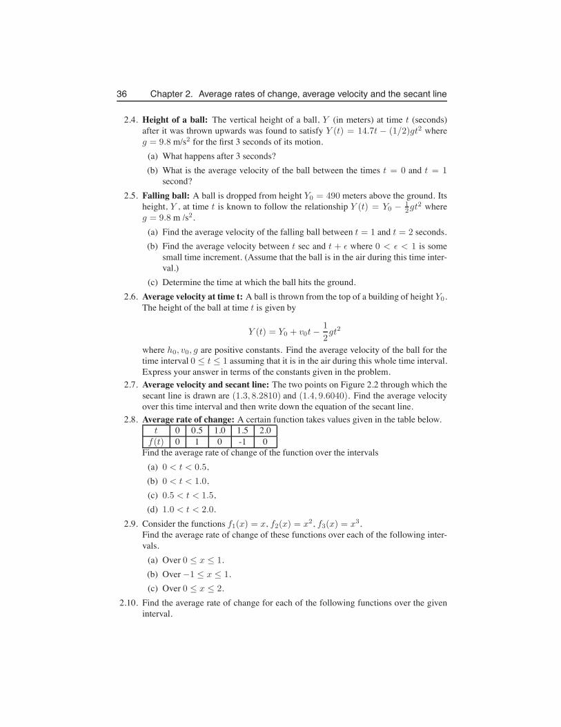
36 Chapter 2. Average rates of change, average velocity and the secant line
2.4. Height of a ball: The vertical height of a ball, Y (in meters) at time t (seconds)after it was thrown upwards was found to satisfy Y (t) = 14.7t − (1/2)gt2 whereg = 9.8 m/s2 for the first 3 seconds of its motion.
(a) What happens after 3 seconds?(b) What is the average velocity of the ball between the times t = 0 and t = 1
second?2.5. Falling ball: A ball is dropped from height Y0 = 490 meters above the ground. Its
height, Y , at time t is known to follow the relationship Y (t) = Y0 − 12gt
2 whereg = 9.8 m /s2.
(a) Find the average velocity of the falling ball between t = 1 and t = 2 seconds.(b) Find the average velocity between t sec and t + ε where 0 < ε < 1 is some
small time increment. (Assume that the ball is in the air during this time inter-val.)
(c) Determine the time at which the ball hits the ground.2.6. Average velocity at time t: A ball is thrown from the top of a building of height Y0.
The height of the ball at time t is given by
Y (t) = Y0 + v0t−1
2gt2
where h0, v0, g are positive constants. Find the average velocity of the ball for thetime interval 0 ≤ t ≤ 1 assuming that it is in the air during this whole time interval.Express your answer in terms of the constants given in the problem.
2.7. Average velocity and secant line: The two points on Figure 2.2 through which thesecant line is drawn are (1.3, 8.2810) and (1.4, 9.6040). Find the average velocityover this time interval and then write down the equation of the secant line.
2.8. Average rate of change: A certain function takes values given in the table below.t 0 0.5 1.0 1.5 2.0
f(t) 0 1 0 -1 0Find the average rate of change of the function over the intervals
(a) 0 < t < 0.5,(b) 0 < t < 1.0,(c) 0.5 < t < 1.5,(d) 1.0 < t < 2.0.
2.9. Consider the functions f1(x) = x, f2(x) = x2, f3(x) = x3.Find the average rate of change of these functions over each of the following inter-vals.
(a) Over 0 ≤ x ≤ 1.(b) Over −1 ≤ x ≤ 1.(c) Over 0 ≤ x ≤ 2.
2.10. Find the average rate of change for each of the following functions over the giveninterval.
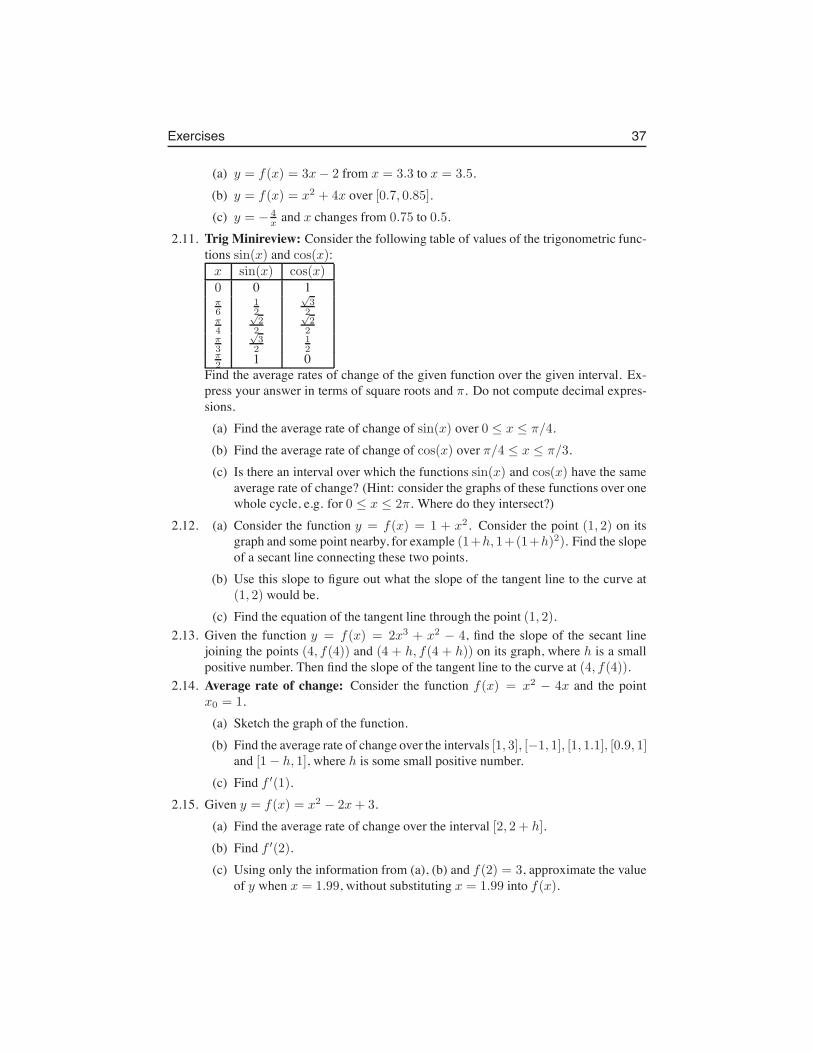
Exercises 37
(a) y = f(x) = 3x− 2 from x = 3.3 to x = 3.5.(b) y = f(x) = x2 + 4x over [0.7, 0.85].(c) y = − 4
x and x changes from 0.75 to 0.5.2.11. Trig Minireview: Consider the following table of values of the trigonometric func-
tions sin(x) and cos(x):x sin(x) cos(x)0 0 1π6
12
√32
π4
√22
√22
π3
√32
12
π2 1 0
Find the average rates of change of the given function over the given interval. Ex-press your answer in terms of square roots and π. Do not compute decimal expres-sions.
(a) Find the average rate of change of sin(x) over 0 ≤ x ≤ π/4.(b) Find the average rate of change of cos(x) over π/4 ≤ x ≤ π/3.(c) Is there an interval over which the functions sin(x) and cos(x) have the same
average rate of change? (Hint: consider the graphs of these functions over onewhole cycle, e.g. for 0 ≤ x ≤ 2π. Where do they intersect?)
2.12. (a) Consider the function y = f(x) = 1 + x2. Consider the point (1, 2) on itsgraph and some point nearby, for example (1+h, 1+(1+h)2). Find the slopeof a secant line connecting these two points.
(b) Use this slope to figure out what the slope of the tangent line to the curve at(1, 2) would be.
(c) Find the equation of the tangent line through the point (1, 2).2.13. Given the function y = f(x) = 2x3 + x2 − 4, find the slope of the secant line
joining the points (4, f(4)) and (4 + h, f(4 + h)) on its graph, where h is a smallpositive number. Then find the slope of the tangent line to the curve at (4, f(4)).
2.14. Average rate of change: Consider the function f(x) = x2 − 4x and the pointx0 = 1.
(a) Sketch the graph of the function.(b) Find the average rate of change over the intervals [1, 3], [−1, 1], [1, 1.1], [0.9, 1]
and [1− h, 1], where h is some small positive number.(c) Find f ′(1).
2.15. Given y = f(x) = x2 − 2x+ 3.(a) Find the average rate of change over the interval [2, 2 + h].(b) Find f ′(2).(c) Using only the information from (a), (b) and f(2) = 3, approximate the value
of y when x = 1.99, without substituting x = 1.99 into f(x).
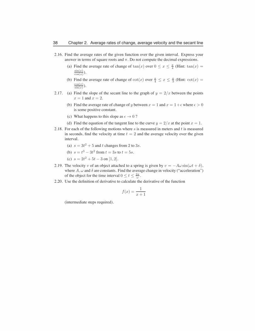
38 Chapter 2. Average rates of change, average velocity and the secant line
2.16. Find the average rates of the given function over the given interval. Express youranswer in terms of square roots and π. Do not compute the decimal expressions.
(a) Find the average rate of change of tan(x) over 0 ≤ x ≤ π4 (Hint: tan(x) =
sin(x)cos(x) ).
(b) Find the average rate of change of cot(x) over π4 ≤ x ≤ π
3 (Hint: cot(x) =cos(x)sin(x) ).
2.17. (a) Find the slope of the secant line to the graph of y = 2/x between the pointsx = 1 and x = 2.
(b) Find the average rate of change of y between x = 1 and x = 1+ε where ε > 0is some positive constant.
(c) What happens to this slope as ε → 0 ?(d) Find the equation of the tangent line to the curve y = 2/x at the point x = 1.
2.18. For each of the following motions where s is measured in meters and t is measuredin seconds, find the velocity at time t = 2 and the average velocity over the giveninterval.
(a) s = 3t2 + 5 and t changes from 2 to 3s.(b) s = t3 − 3t2 from t = 3s to t = 5s.(c) s = 2t2 + 5t− 3 on [1, 2].
2.19. The velocity v of an object attached to a spring is given by v = −Aω sin(ωt + δ),where A, ω and δ are constants. Find the average change in velocity (“acceleration”)of the object for the time interval 0 ≤ t ≤ 2π
ω .2.20. Use the definition of derivative to calculate the derivative of the function
f(x) =1
x+ 1
(intermediate steps required).
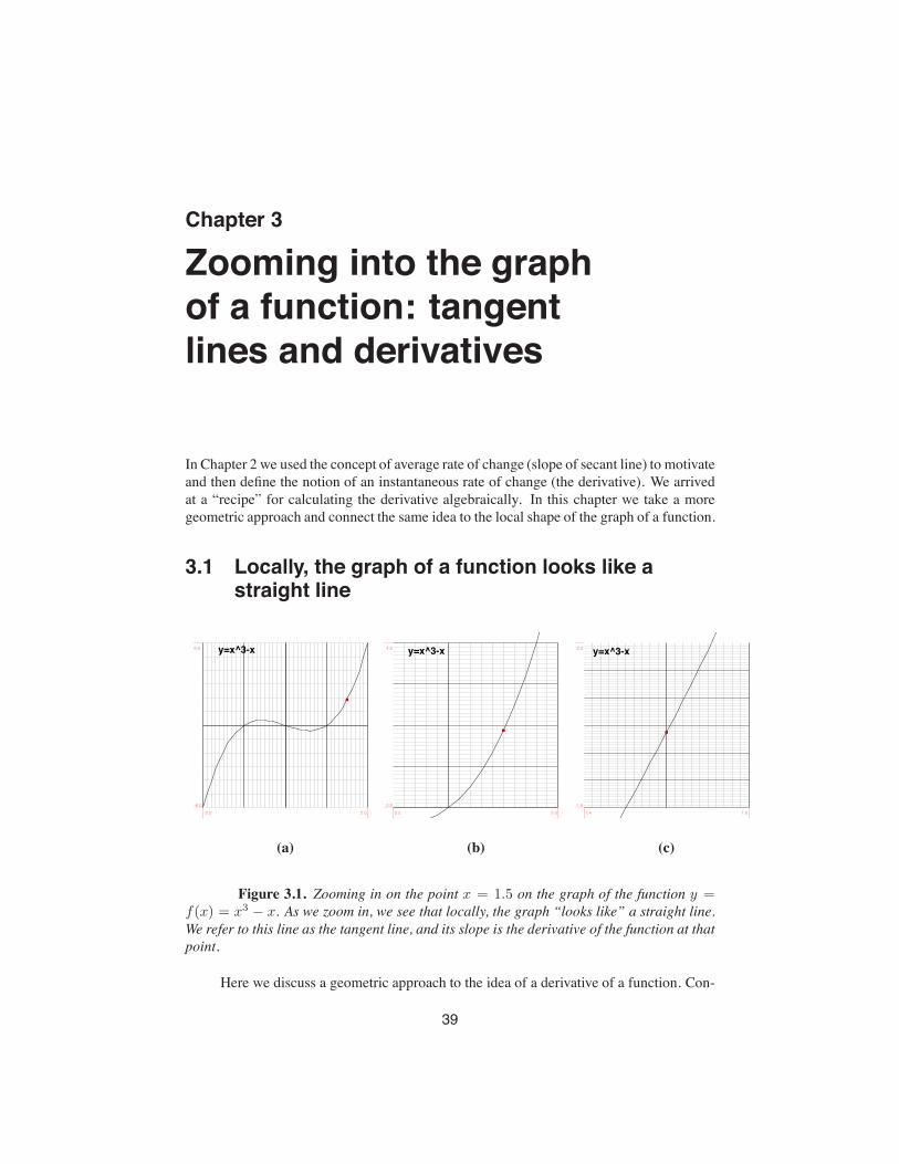
Chapter 3
Zooming into the graphof a function: tangentlines and derivatives
In Chapter 2 we used the concept of average rate of change (slope of secant line) to motivateand then define the notion of an instantaneous rate of change (the derivative). We arrivedat a “recipe” for calculating the derivative algebraically. In this chapter we take a moregeometric approach and connect the same idea to the local shape of the graph of a function.
3.1 Locally, the graph of a function looks like astraight line
y=x^3-x
-2.0 2.0-6.0
6.0 y=x^3-x
0.5 2.00.0
4.0 y=x^3-x
1.4 1.61.6
2.2
(a) (b) (c)
Figure 3.1. Zooming in on the point x = 1.5 on the graph of the function y =f(x) = x3 − x. As we zoom in, we see that locally, the graph “looks like” a straight line.We refer to this line as the tangent line, and its slope is the derivative of the function at thatpoint.
Here we discuss a geometric approach to the idea of a derivative of a function. Con-
39
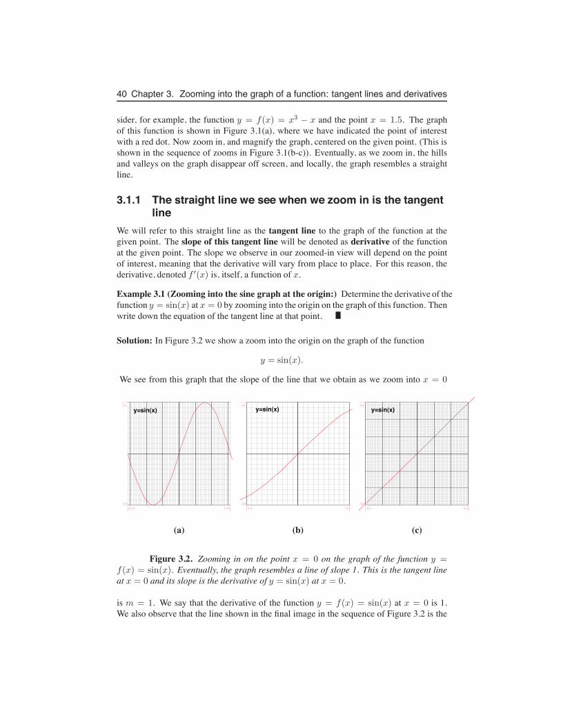
40 Chapter 3. Zooming into the graph of a function: tangent lines and derivatives
sider, for example, the function y = f(x) = x3 − x and the point x = 1.5. The graphof this function is shown in Figure 3.1(a), where we have indicated the point of interestwith a red dot. Now zoom in, and magnify the graph, centered on the given point. (This isshown in the sequence of zooms in Figure 3.1(b-c)). Eventually, as we zoom in, the hillsand valleys on the graph disappear off screen, and locally, the graph resembles a straightline.
3.1.1 The straight line we see when we zoom in is the tangentline
We will refer to this straight line as the tangent line to the graph of the function at thegiven point. The slope of this tangent line will be denoted as derivative of the functionat the given point. The slope we observe in our zoomed-in view will depend on the pointof interest, meaning that the derivative will vary from place to place. For this reason, thederivative, denoted f ′(x) is, itself, a function of x.
Example 3.1 (Zooming into the sine graph at the origin:) Determine the derivative of thefunction y = sin(x) at x = 0 by zooming into the origin on the graph of this function. Thenwrite down the equation of the tangent line at that point.
Solution: In Figure 3.2 we show a zoom into the origin on the graph of the function
y = sin(x).
We see from this graph that the slope of the line that we obtain as we zoom into x = 0
y=sin(x)
-3.14 3.14-1.0
1.0y=sin(x)
-1.0 1.0-1.0
1.0
y=sin(x)
-0.3 0.3-0.3
0.3
(a) (b) (c)
Figure 3.2. Zooming in on the point x = 0 on the graph of the function y =f(x) = sin(x). Eventually, the graph resembles a line of slope 1. This is the tangent lineat x = 0 and its slope is the derivative of y = sin(x) at x = 0.
is m = 1. We say that the derivative of the function y = f(x) = sin(x) at x = 0 is 1.We also observe that the line shown in the final image in the sequence of Figure 3.2 is the
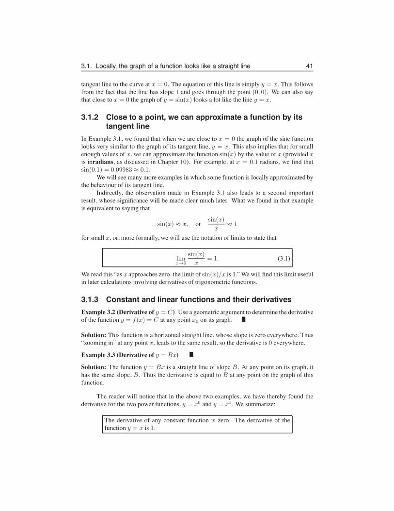
3.1. Locally, the graph of a function looks like a straight line 41
tangent line to the curve at x = 0. The equation of this line is simply y = x. This followsfrom the fact that the line has slope 1 and goes through the point (0, 0). We can also saythat close to x = 0 the graph of y = sin(x) looks a lot like the line y = x.
3.1.2 Close to a point, we can approximate a function by itstangent line
In Example 3.1, we found that when we are close to x = 0 the graph of the sine functionlooks very similar to the graph of its tangent line, y = x. This also implies that for smallenough values of x, we can approximate the function sin(x) by the value of x (provided xis inradians, as discussed in Chapter 10). For example, at x = 0.1 radians, we find thatsin(0.1) = 0.09983 ≈ 0.1.
We will see many more examples in which some function is locally approximated bythe behaviour of its tangent line.
Indirectly, the observation made in Example 3.1 also leads to a second importantresult, whose significance will be made clear much later. What we found in that exampleis equivalent to saying that
sin(x) ≈ x, or sin(x)
x≈ 1
for small x, or, more formally, we will use the notation of limits to state that
limx→0
sin(x)
x= 1. (3.1)
We read this “as x approaches zero, the limit of sin(x)/x is 1.” We will find this limit usefulin later calculations involving derivatives of trigonometric functions.
3.1.3 Constant and linear functions and their derivativesExample 3.2 (Derivative of y = C) Use a geometric argument to determine the derivativeof the function y = f(x) = C at any point x0 on its graph.
Solution: This function is a horizontal straight line, whose slope is zero everywhere. Thus“zooming in” at any point x, leads to the same result, so the derivative is 0 everywhere.
Example 3.3 (Derivative of y = Bx)
Solution: The function y = Bx is a straight line of slope B. At any point on its graph, ithas the same slope, B. Thus the derivative is equal to B at any point on the graph of thisfunction.
The reader will notice that in the above two examples, we have thereby found thederivative for the two power functions, y = x0 and y = x1. We summarize:
The derivative of any constant function is zero. The derivative of thefunction y = x is 1.
42 Chapter 3. Zooming into the graph of a function: tangent lines and derivatives
3.2 Equation of a tangent line
y=sin(x)
-3.14 3.14-1.5
1.5
y=sin(x)
1.5 1.640.98
1.01
y=sin(x)
1.56 1.580.99
1.01
(a) (b) (c)
Figure 3.3. Here we zoom in on the point x = π/2 on the graph of y = f(x) =sin(x). This point is a “local maximum”. Eventually, we see the tangent line whose slopeis 0 (it is is horizontal). Thus the derivative of y = sin(x) at x = π/2 is zero.
The examples above allow us to visualize the tangent line by examining the local(“zoomed in”) shape of the function. In two examples, we found the slope of that tangentline, which is identified by the derivative of the function at the given point. Using suchinformation, we can write down the equation of that tangent line.
Example 3.4 (Zooming in at π/2:) Find the equation of the tangent line to the graph ofy = sin(x) at the point x = π/2.
Solution:In the zooms shown in Fig. 3.3, we observe that the tangent line to y = sin(x) at the
point x = π/2 is horizontal (equivalent to saying it has slope 0). That line goes throughthe point (π/2, sin(π/2)) = (π/2, 1). Since the line is horizontal, its y value is constanteverywhere, so that the equation of this line is simply y = 1.
Example 3.5 Find the equation of the tangent line to the graph of y = f(x) = x3 − x atthe point x = 1.5 shown in Fig. 3.1.
Solution: The point of interest has coordinates (x, f(x)) = (1.5, 1.875). From the graphshown in Fig. 3.1 (c) we see that the “tangent line” approximately goes through (1.7, 1.47)as well as the red point (1.5, 1.875). We can compute its slope and find it to be approx-imately ∆y/∆x ≈ 5.8. To find the equation of the tangent line, we use this slope and apoint on that line to write
y − 1.875
x− 1.5= 5.8 ⇒ y = 1.875 + 5.8(x− 1.5) ⇒ y = 5.8x− 6.825
Later, we will use the (analytic) definition of the derivative and an exact algebraic calcula-tion to improve on this result.
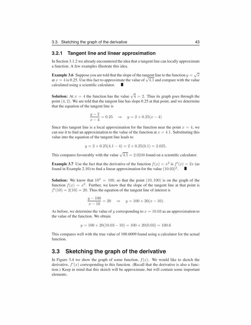
3.3. Sketching the graph of the derivative 43
3.2.1 Tangent line and linear approximationIn Section 3.1.2 we already encountered the idea that a tangent line can locally approximatea function. A few examples illustrate this idea.
Example 3.6 Suppose you are told that the slope of the tangent line to the function y =√x
at x = 4 is 0.25. Use this fact to approximate the value of√4.1 and compare with the value
calculated using a scientific calculator.
Solution: At x = 4 the function has the value√4 = 2. Thus its graph goes through the
point (4, 2). We are told that the tangent line has slope 0.25 at that point, and we determinethat the equation of the tangent line is
y − 2
x− 4= 0.25 ⇒ y = 2 + 0.25(x− 4)
Since this tangent line is a local approximation for the function near the point x = 4, wecan use it to find an approximation to the value of the function at x = 4.1. Substituting thisvalue into the equation of the tangent line leads to
y = 2 + 0.25(4.1− 4) = 2 + 0.25(0.1) = 2.025.
This compares favourably with the value√4.1 = 2.0248 found on a scientific calculator.
Example 3.7 Use the fact that the derivative of the function f(x) = x2 is f ′(x) = 2x (asfound in Example 2.10) to find a linear approximation for the value (10.03)2.
Solution: We know that 102 = 100, so that the point (10, 100) is on the graph of thefunction f(x) = x2. Further, we know that the slope of the tangent line at that point isf ′(10) = 2(10) = 20. Thus the equation of the tangent line of interest is
y − 100
x− 10= 20 ⇒ y = 100 + 20(x− 10).
As before, we determine the value of y corresponding to x = 10.03 as an approximation tothe value of the function. We obtain
y = 100 + 20(10.03− 10) = 100 + 20(0.03) = 100.6
This compares well with the true value of 100.6009 found using a calculator for the actualfunction.
3.3 Sketching the graph of the derivativeIn Figure 3.4 we show the graph of some function, f(x). We would like to sketch thederivative, f ′(x) corresponding to this function. (Recall that the derivative is also a func-tion.) Keep in mind that this sketch will be approximate, but will contain some importantelements.
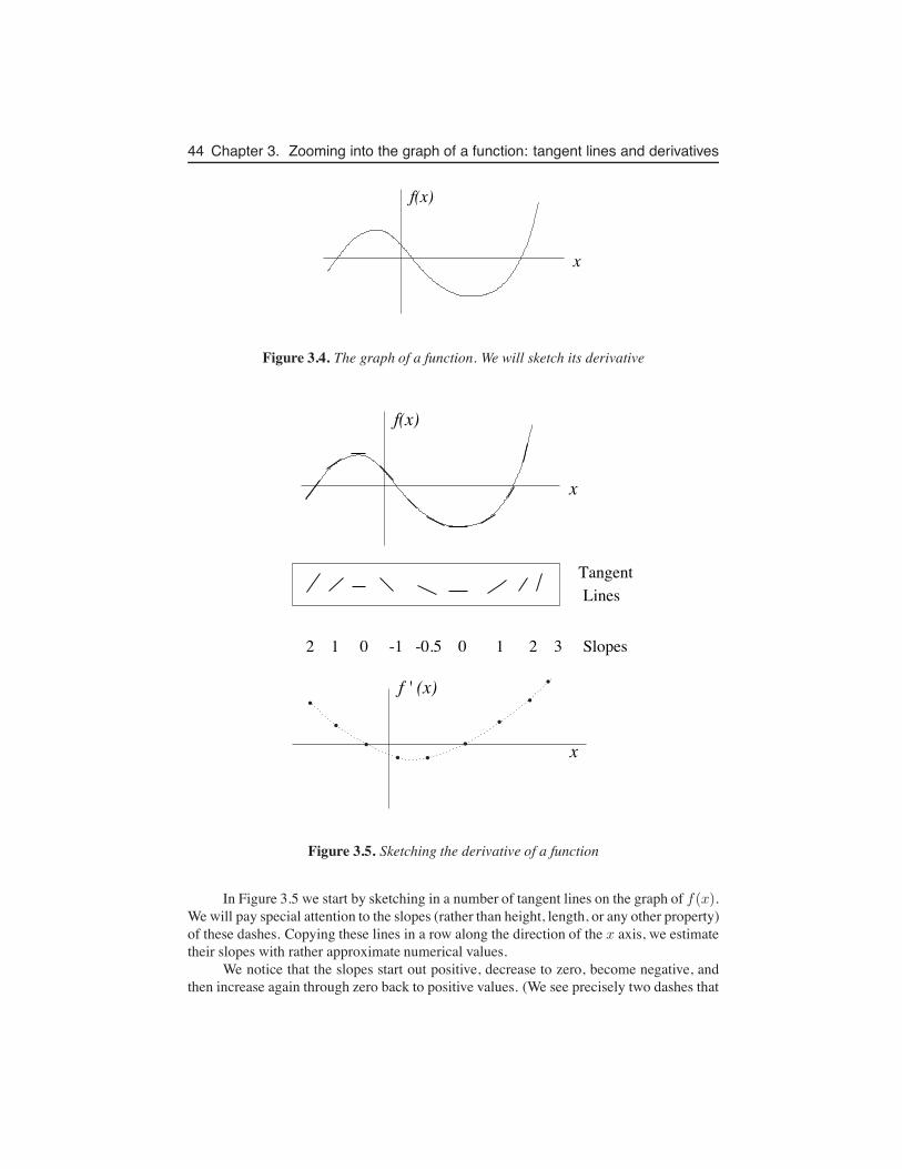
44 Chapter 3. Zooming into the graph of a function: tangent lines and derivatives
x
f(x)
Figure 3.4. The graph of a function. We will sketch its derivative
x
f(x)
Tangent
Lines
2 1 0 -1 -0.5 0 1 2 3 Slopes
x
f ' (x)
Figure 3.5. Sketching the derivative of a function
In Figure 3.5 we start by sketching in a number of tangent lines on the graph of f(x).We will pay special attention to the slopes (rather than height, length, or any other property)of these dashes. Copying these lines in a row along the direction of the x axis, we estimatetheir slopes with rather approximate numerical values.
We notice that the slopes start out positive, decrease to zero, become negative, andthen increase again through zero back to positive values. (We see precisely two dashes that
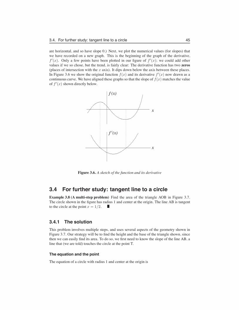
3.4. For further study: tangent line to a circle 45
are horizontal, and so have slope 0.) Next, we plot the numerical values (for slopes) thatwe have recorded on a new graph. This is the beginning of the graph of the derivative,f ′(x). Only a few points have been plotted in our figure of f ′(x); we could add othervalues if we so chose, but the trend, is fairly clear: The derivative function has two zeros(places of intersection with the x axis). It dips down below the axis between these places.In Figure 3.6 we show the original function f(x) and its derivative f ′(x) now drawn as acontinuous curve. We have aligned these graphs so that the slope of f(x) matches the valueof f ′(x) shown directly below.
x
f (x)
x
f (x)
Figure 3.6. A sketch of the function and its derivative
3.4 For further study: tangent line to a circleExample 3.8 (A multi-step problem) Find the area of the triangle AOB in Figure 3.7.The circle shown in the figure has radius 1 and center at the origin. The line AB is tangentto the circle at the point x = 1/2.
3.4.1 The solutionThis problem involves multiple steps, and uses several aspects of the geometry shown inFigure 3.7. Our strategy will be to find the height and the base of the triangle shown, sincethen we can easily find its area. To do so, we first need to know the slope of the line AB, aline that (we are told) touches the circle at the point T.
The equation and the point
The equation of a circle with radius 1 and center at the origin is
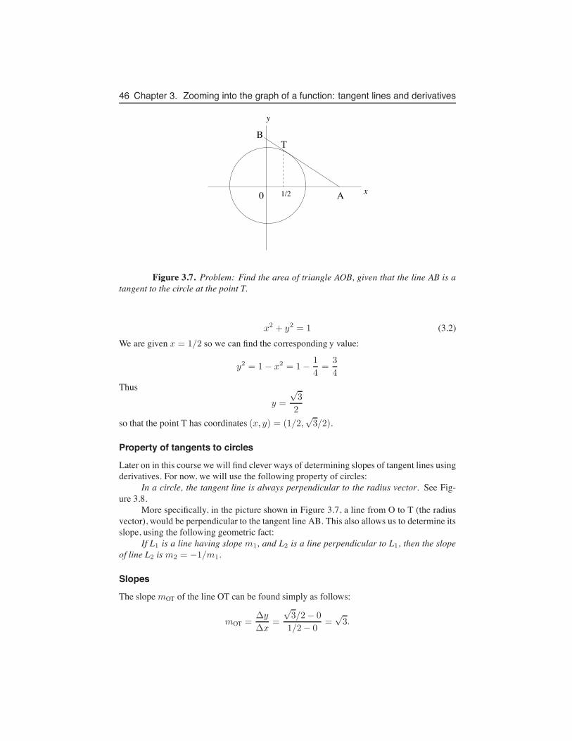
46 Chapter 3. Zooming into the graph of a function: tangent lines and derivatives
y
B
0 xA1/2
T
Figure 3.7. Problem: Find the area of triangle AOB, given that the line AB is atangent to the circle at the point T.
x2 + y2 = 1 (3.2)We are given x = 1/2 so we can find the corresponding y value:
y2 = 1− x2 = 1−1
4=
3
4
Thus
y =
√3
2
so that the point T has coordinates (x, y) = (1/2,√3/2).
Property of tangents to circles
Later on in this course we will find clever ways of determining slopes of tangent lines usingderivatives. For now, we will use the following property of circles:
In a circle, the tangent line is always perpendicular to the radius vector. See Fig-ure 3.8.
More specifically, in the picture shown in Figure 3.7, a line from O to T (the radiusvector), would be perpendicular to the tangent line AB. This also allows us to determine itsslope, using the following geometric fact:
If L1 is a line having slope m1, and L2 is a line perpendicular to L1, then the slopeof line L2 is m2 = −1/m1.
Slopes
The slope mOT of the line OT can be found simply as follows:
mOT =∆y
∆x=
√3/2− 0
1/2− 0=
√3.
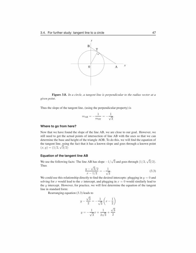
3.4. For further study: tangent line to a circle 47
y
B
0 xA
T
Figure 3.8. In a circle, a tangent line is perpendicular to the radius vector at agiven point.
Thus the slope of the tangent line, (using the perpendicular property) is
mAB = −1
mOT= −
1√3.
Where to go from here?
Now that we have found the slope of the line AB, we are close to our goal. However, westill need to get the actual points of intersection of line AB with the axes so that we candetermine the base and height of the triangle AOB. To do this, we will find the equation ofthe tangent line, using the fact that it has a known slope and goes through a known point(x, y) = (1/2,
√3/2)
Equation of the tangent line AB
We use the following facts: The line AB has slope −1/√3 and goes through (1/2,
√3/2).
Thusy −
√3/2
x− 1/2= −
1√3. (3.3)
We could use this relationship directly to find the desired intercepts: plugging in y = 0 andsolving for x would lead to the x intercept, and plugging in x = 0 would similarly lead tothe y intercept. However, for practice, we will first determine the equation of the tangentline in standard form:
Rearranging equation (3.3) leads to
y −√3
2= −
1√3
(
x−1
2
)
y = −1√3x+
1
2√3+
√3
2
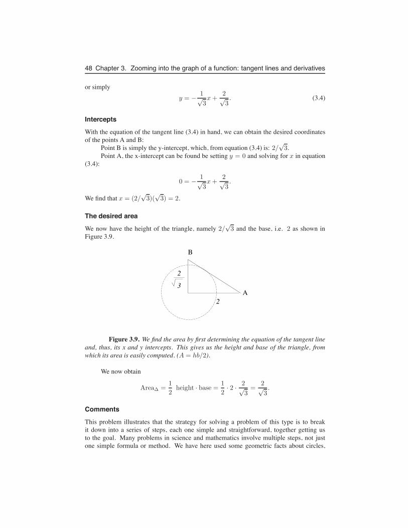
48 Chapter 3. Zooming into the graph of a function: tangent lines and derivatives
or simplyy = −
1√3x+
2√3. (3.4)
Intercepts
With the equation of the tangent line (3.4) in hand, we can obtain the desired coordinatesof the points A and B:
Point B is simply the y-intercept, which, from equation (3.4) is: 2/√3.
Point A, the x-intercept can be found be setting y = 0 and solving for x in equation(3.4):
0 = −1√3x+
2√3.
We find that x = (2/√3)(
√3) = 2.
The desired area
We now have the height of the triangle, namely 2/√3 and the base, i.e. 2 as shown in
Figure 3.9.
A
B
3
2
2
Figure 3.9. We find the area by first determining the equation of the tangent lineand, thus, its x and y intercepts. This gives us the height and base of the triangle, fromwhich its area is easily computed. (A = hb/2).
We now obtain
Area∆ =1
2height · base =
1
2· 2 ·
2√3=
2√3.
Comments
This problem illustrates that the strategy for solving a problem of this type is to breakit down into a series of steps, each one simple and straightforward, together getting usto the goal. Many problems in science and mathematics involve multiple steps, not justone simple formula or method. We have here used some geometric facts about circles,
3.4. For further study: tangent line to a circle 49
some knowledge of properties of slopes and straight lines, as well as simple algebraicmanipulations to get to our final destination.
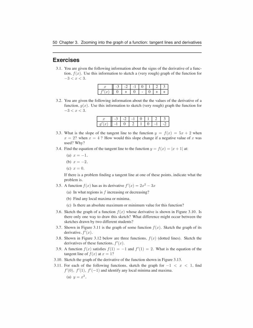
50 Chapter 3. Zooming into the graph of a function: tangent lines and derivatives
Exercises3.1. You are given the following information about the signs of the derivative of a func-
tion, f(x). Use this information to sketch a (very rough) graph of the function for−3 < x < 3.
x -3 -2 -1 0 1 2 3f ′(x) 0 + 0 - 0 + +
3.2. You are given the following information about the the values of the derivative of afunction, g(x). Use this information to sketch (very rough) graph the function for−3 < x < 3.
x -3 -2 -1 0 1 2 3g′(x) -1 0 2 1 0 -1 -2
3.3. What is the slope of the tangent line to the function y = f(x) = 5x + 2 whenx = 2? when x = 4 ? How would this slope change if a negative value of x wasused? Why?
3.4. Find the equation of the tangent line to the function y = f(x) = |x+ 1| at:(a) x = −1,(b) x = −2,(c) x = 0.
If there is a problem finding a tangent line at one of these points, indicate what theproblem is.
3.5. A function f(x) has as its derivative f ′(x) = 2x2 − 3x
(a) In what regions is f increasing or decreasing?(b) Find any local maxima or minima.(c) Is there an absolute maximum or minimum value for this function?
3.6. Sketch the graph of a function f(x) whose derivative is shown in Figure 3.10. Isthere only one way to draw this sketch? What difference might occur between thesketches drawn by two different students?
3.7. Shown in Figure 3.11 is the graph of some function f(x). Sketch the graph of itsderivative, f ′(x).
3.8. Shown in Figure 3.12 below are three functions, f(x) (dotted lines). Sketch thederivatives of these functions, f ′(x).
3.9. A function f(x) satisfies f(1) = −1 and f ′(1) = 2. What is the equation of thetangent line of f(x) at x = 1?
3.10. Sketch the graph of the derivative of the function shown in Figure 3.13.3.11. For each of the following functions, sketch the graph for −1 < x < 1, find
f ′(0), f ′(1), f ′(−1) and identify any local minima and maxima.(a) y = x2,
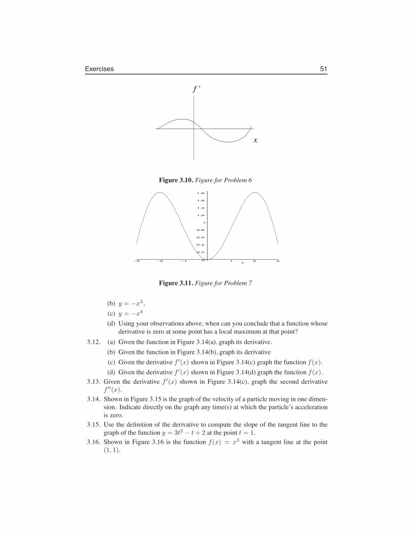
Exercises 51
x
f ’
Figure 3.10. Figure for Problem 6
0
0.2
0.4
0.6
0.8
1
1.2
1.4
1.6
1.8
–3 –2 –1 1 2 3x
Figure 3.11. Figure for Problem 7
(b) y = −x3,(c) y = −x4
(d) Using your observations above, when can you conclude that a function whosederivative is zero at some point has a local maximum at that point?
3.12. (a) Given the function in Figure 3.14(a), graph its derivative.(b) Given the function in Figure 3.14(b), graph its derivative(c) Given the derivative f ′(x) shown in Figure 3.14(c) graph the function f(x).(d) Given the derivative f ′(x) shown in Figure 3.14(d) graph the function f(x).
3.13. Given the derivative f ′(x) shown in Figure 3.14(c), graph the second derivativef ′′(x).
3.14. Shown in Figure 3.15 is the graph of the velocity of a particle moving in one dimen-sion. Indicate directly on the graph any time(s) at which the particle’s accelerationis zero.
3.15. Use the definition of the derivative to compute the slope of the tangent line to thegraph of the function y = 3t2 − t+ 2 at the point t = 1.
3.16. Shown in Figure 3.16 is the function f(x) = x3 with a tangent line at the point(1, 1).
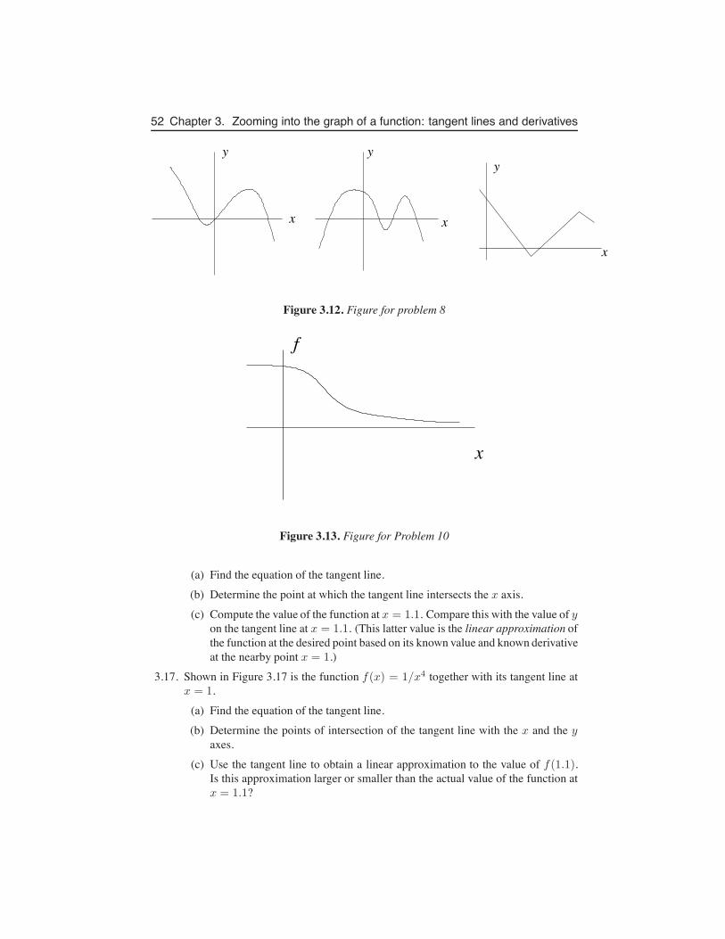
52 Chapter 3. Zooming into the graph of a function: tangent lines and derivatives
x x
x
y yy
Figure 3.12. Figure for problem 8
x
f
Figure 3.13. Figure for Problem 10
(a) Find the equation of the tangent line.(b) Determine the point at which the tangent line intersects the x axis.(c) Compute the value of the function at x = 1.1. Compare this with the value of y
on the tangent line at x = 1.1. (This latter value is the linear approximation ofthe function at the desired point based on its known value and known derivativeat the nearby point x = 1.)
3.17. Shown in Figure 3.17 is the function f(x) = 1/x4 together with its tangent line atx = 1.
(a) Find the equation of the tangent line.(b) Determine the points of intersection of the tangent line with the x and the y
axes.(c) Use the tangent line to obtain a linear approximation to the value of f(1.1).
Is this approximation larger or smaller than the actual value of the function atx = 1.1?
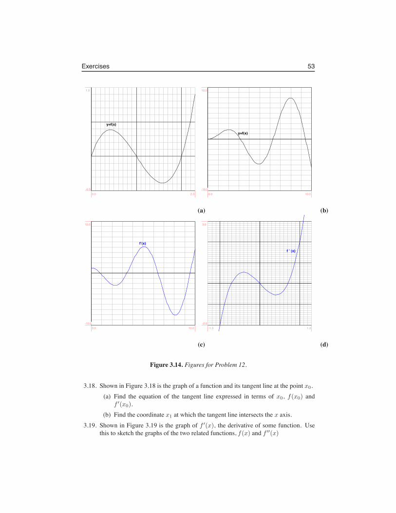
Exercises 53
y=f(x)
0.0 2.3-0.5
1.0
y=f(x)
0.0 10.0-10.0
10.0
(a) (b)
f’(x)
0.0 10.0-10.0
10.0
f ’ (x)
-1.3 1.3-2.0
3.0
(c) (d)
Figure 3.14. Figures for Problem 12.
3.18. Shown in Figure 3.18 is the graph of a function and its tangent line at the point x0.(a) Find the equation of the tangent line expressed in terms of x0, f(x0) and
f ′(x0).(b) Find the coordinate x1 at which the tangent line intersects the x axis.
3.19. Shown in Figure 3.19 is the graph of f ′(x), the derivative of some function. Usethis to sketch the graphs of the two related functions, f(x) and f ′′(x)
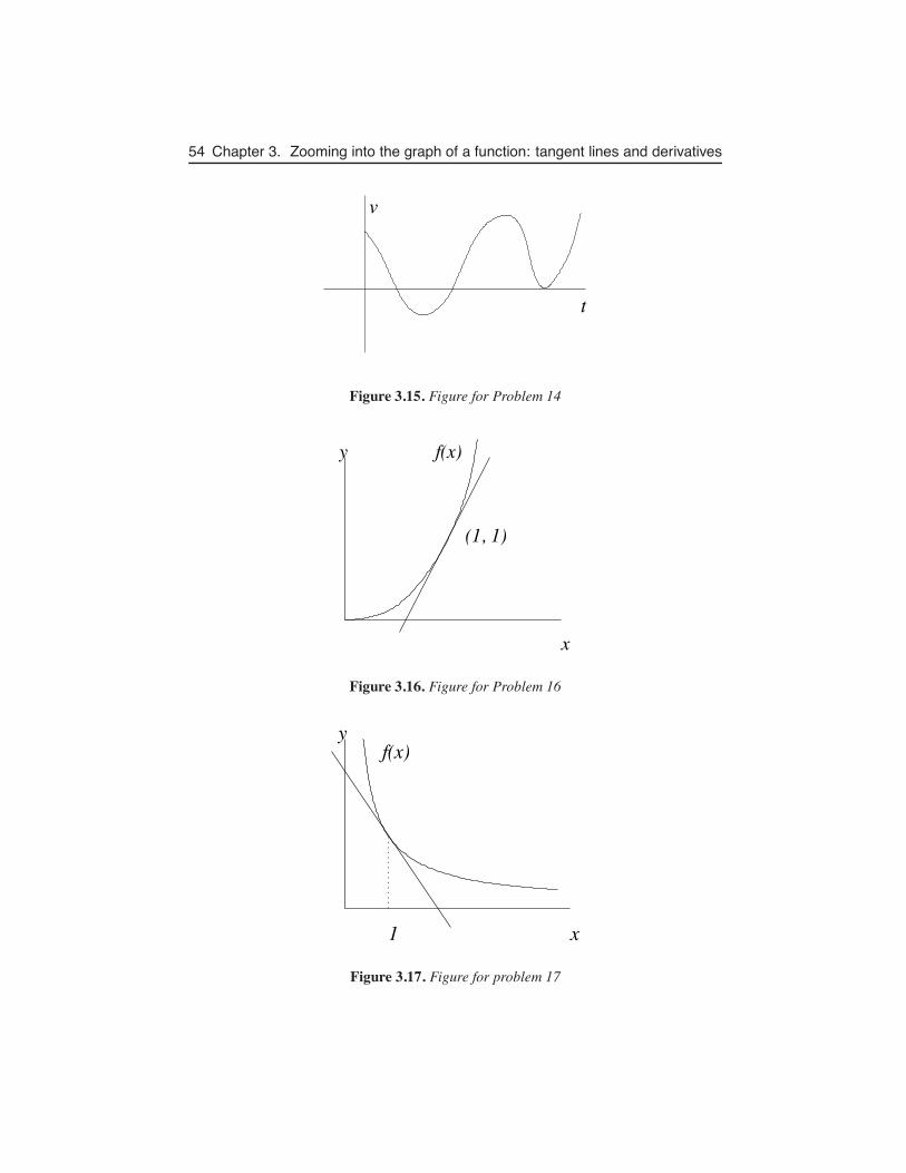
54 Chapter 3. Zooming into the graph of a function: tangent lines and derivatives
v
t
Figure 3.15. Figure for Problem 14
x
y
(1, 1)
f(x)
Figure 3.16. Figure for Problem 16
x
yf(x)
1
Figure 3.17. Figure for problem 17
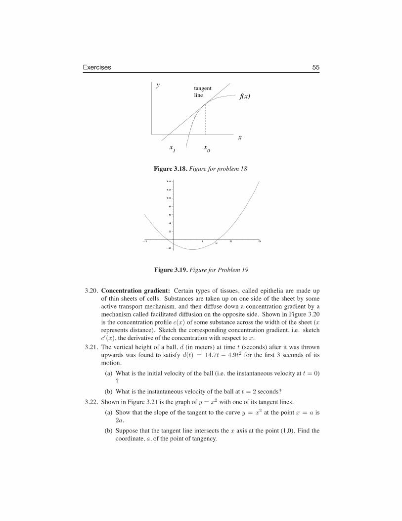
Exercises 55
x
yf(x)
xx1 0
tangentline
Figure 3.18. Figure for problem 18
–2
2
4
6
8
10
12
14
–1 1 2 3x
Figure 3.19. Figure for Problem 19
3.20. Concentration gradient: Certain types of tissues, called epithelia are made upof thin sheets of cells. Substances are taken up on one side of the sheet by someactive transport mechanism, and then diffuse down a concentration gradient by amechanism called facilitated diffusion on the opposite side. Shown in Figure 3.20is the concentration profile c(x) of some substance across the width of the sheet (xrepresents distance). Sketch the corresponding concentration gradient, i.e. sketchc′(x), the derivative of the concentration with respect to x.
3.21. The vertical height of a ball, d (in meters) at time t (seconds) after it was thrownupwards was found to satisfy d(t) = 14.7t − 4.9t2 for the first 3 seconds of itsmotion.
(a) What is the initial velocity of the ball (i.e. the instantaneous velocity at t = 0)?
(b) What is the instantaneous velocity of the ball at t = 2 seconds?3.22. Shown in Figure 3.21 is the graph of y = x2 with one of its tangent lines.
(a) Show that the slope of the tangent to the curve y = x2 at the point x = a is2a.
(b) Suppose that the tangent line intersects the x axis at the point (1,0). Find thecoordinate, a, of the point of tangency.
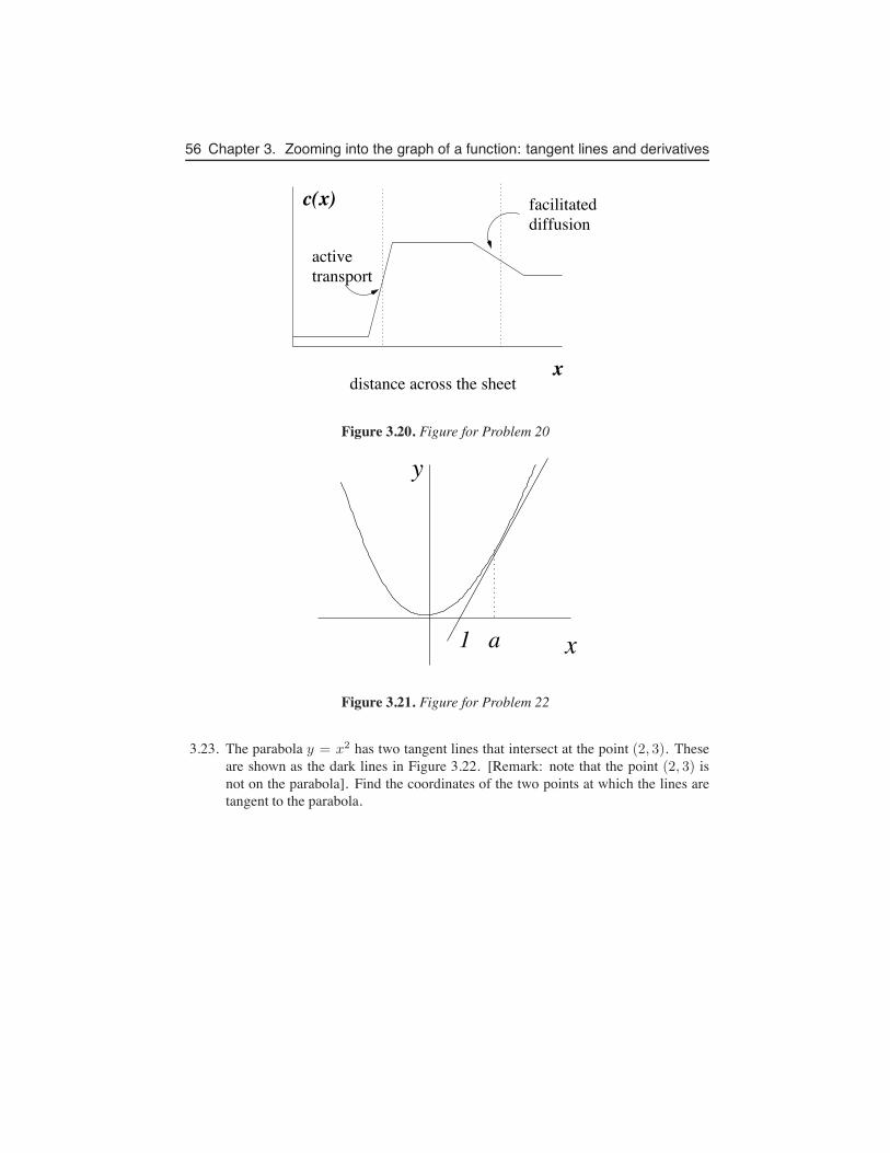
56 Chapter 3. Zooming into the graph of a function: tangent lines and derivatives
x
c(x) facilitateddiffusion
activetransport
distance across the sheet
Figure 3.20. Figure for Problem 20
x
y
1 a
Figure 3.21. Figure for Problem 22
3.23. The parabola y = x2 has two tangent lines that intersect at the point (2, 3). Theseare shown as the dark lines in Figure 3.22. [Remark: note that the point (2, 3) isnot on the parabola]. Find the coordinates of the two points at which the lines aretangent to the parabola.
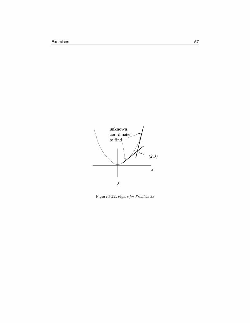
Exercises 57
unknowncoordinatesto find
(2,3)
x
y
Figure 3.22. Figure for Problem 23

58 Chapter 3. Zooming into the graph of a function: tangent lines and derivatives
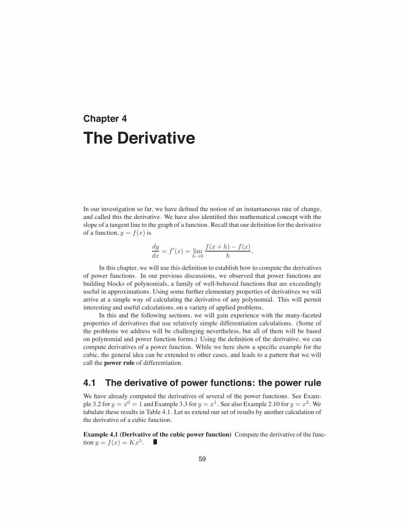
Chapter 4
The Derivative
In our investigation so far, we have defined the notion of an instantaneous rate of change,and called this the derivative. We have also identified this mathematical concept with theslope of a tangent line to the graph of a function. Recall that our definition for the derivativeof a function, y = f(x) is
dy
dx= f ′(x) = lim
h→0
f(x+ h)− f(x)
h.
In this chapter, we will use this definition to establish how to compute the derivativesof power functions. In our previous discussions, we observed that power functions arebuilding blocks of polynomials, a family of well-behaved functions that are exceedinglyuseful in approximations. Using some further elementary properties of derivatives we willarrive at a simple way of calculating the derivative of any polynomial. This will permitinteresting and useful calculations, on a variety of applied problems.
In this and the following sections, we will gain experience with the many-facetedproperties of derivatives that use relatively simple differentiation calculations. (Some ofthe problems we address will be challenging nevertheless, but all of them will be basedon polynomial and power function forms.) Using the definition of the derivative, we cancompute derivatives of a power function. While we here show a specific example for thecubic, the general idea can be extended to other cases, and leads to a pattern that we willcall the power rule of differentiation.
4.1 The derivative of power functions: the power ruleWe have already computed the derivatives of several of the power functions. See Exam-ple 3.2 for y = x0 = 1 and Example 3.3 for y = x1. See also Example 2.10 for y = x2. Wetabulate these results in Table 4.1. Let us extend our set of results by another calculation ofthe derivative of a cubic function.
Example 4.1 (Derivative of the cubic power function) Compute the derivative of the func-tion y = f(x) = Kx3.
59
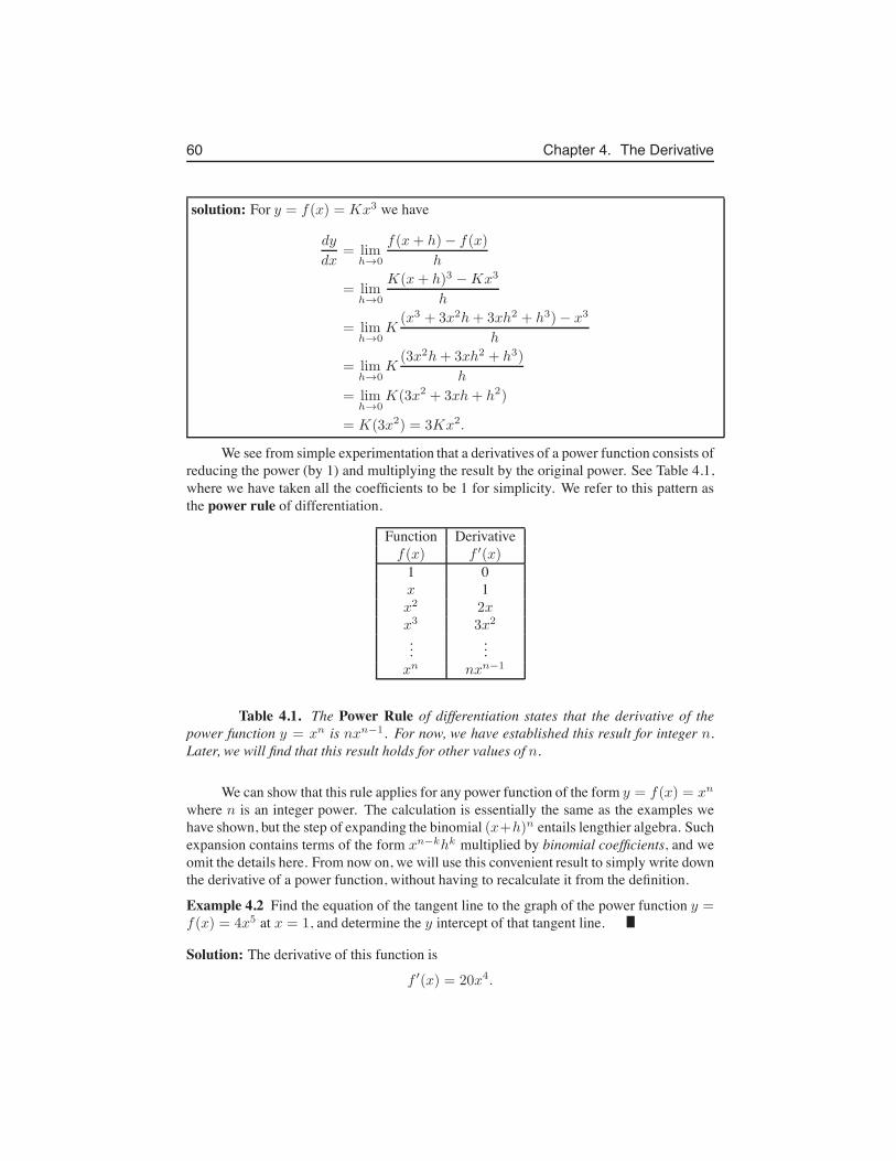
60 Chapter 4. The Derivative
solution: For y = f(x) = Kx3 we have
dy
dx= lim
h→0
f(x+ h)− f(x)
h
= limh→0
K(x+ h)3 −Kx3
h
= limh→0
K(x3 + 3x2h+ 3xh2 + h3)− x3
h
= limh→0
K(3x2h+ 3xh2 + h3)
h
= limh→0
K(3x2 + 3xh+ h2)
= K(3x2) = 3Kx2.
We see from simple experimentation that a derivatives of a power function consists ofreducing the power (by 1) and multiplying the result by the original power. See Table 4.1,where we have taken all the coefficients to be 1 for simplicity. We refer to this pattern asthe power rule of differentiation.
Function Derivativef(x) f ′(x)
1 0x 1x2 2xx3 3x2
......
xn nxn−1
Table 4.1. The Power Rule of differentiation states that the derivative of thepower function y = xn is nxn−1. For now, we have established this result for integer n.Later, we will find that this result holds for other values of n.
We can show that this rule applies for any power function of the form y = f(x) = xn
where n is an integer power. The calculation is essentially the same as the examples wehave shown, but the step of expanding the binomial (x+h)n entails lengthier algebra. Suchexpansion contains terms of the form xn−khk multiplied by binomial coefficients, and weomit the details here. From now on, we will use this convenient result to simply write downthe derivative of a power function, without having to recalculate it from the definition.
Example 4.2 Find the equation of the tangent line to the graph of the power function y =f(x) = 4x5 at x = 1, and determine the y intercept of that tangent line.
Solution: The derivative of this function is
f ′(x) = 20x4.
4.2. The derivative is a linear operation 61
At the point x = 1, we have dy/dx = f ′(1) = 20 and y = f(1) = 4. This means that thetangent line goes through the point (1, 4) and has slope 20. Thus, its equation is
y − 4
x− 1= 20
y = 4 + 20(x− 1) = 20x− 16.
(At this point is is a good idea to do a quick check that the point (1, 4) satisfies this equation,and that the slope of the line is 20.) Thus, we find that the y intercept of the tangent line isy = −16.
Next, we find that the result for derivatives of power functions can be extended to deriva-tives of polynomials, using further simple properties of the derivative.
4.2 The derivative is a linear operationThe derivative satisfies several convenient properties: The sum of two functions or the con-stant multiple of a function has a derivative that is related simply to the original function(s).The derivative of a sum is the same as the sum of the derivatives. A constant multiple of afunction can be brought outside the differentiation.
d
dx(f(x) + g(x)) =
df
dx+
dg
dx(4.1)
d
dxCf(x) = C
df
dx(4.2)
We can summarize these observations by saying that the derivative is a linear oper-ation. In general, a linear operation L is a rule or process that satisfies two properties: (1)L[f + g] = L[f ] + L[g] and L[cf ] = cL[f ], where f, g are objects (such as functions,vectors, etc) on which L acts, and c is a constant multiple. We will refer to (4.1) and (4.2)as the “linearity” properties of the derivative.
4.3 The derivative of a polynomialUsing the properties (4.1) and (4.2), we can extend our differentiation power rule to com-pute the derivative of any polynomial. Recall that polynomials are sums of power functionsmultiplied by constants. A polynomial of degree n has the form
p(x) = anxn + an−1x
n−1 + . . . a1x+ a0 (4.3)
where the coefficients, ai are constant and n is an integer. Thus, by the above two prop-erties, the derivative of a polynomial is just the sum of derivatives of power functions(multiplied by constants). Thus the derivative of (4.3) is
p′(x) =dy
dx= an · nxn−1 + an−1 · (n− 1)xn−2 + . . . a1 (4.4)
62 Chapter 4. The Derivative
(Observe that each term consists of the coefficient times the derivative of a power functions.The constant term a0 has disappeared since the derivative of any constant is zero.) Thederivative, p′(x), is apparently also a function, and a polynomial as well. Its degree isn − 1, one less than that of p(x). In view of this observation, we could ask what is thederivative of the derivative, which we henceforth call the second derivative., written inthe notation p′′(x) or, equivalently d2y
dx2 . Using the same rules, we can compute this easily,obtaining
p′′(x) =d2y
dx2= an · n(n− 1)xn−2 + an−1 · (n− 1) · (n− 2)xn−3 + . . . a2 (4.5)
We demonstrate the idea with a few examples
Example 4.3 Find the first and second derivatives of the function (a) y = f(x) = 2x5 +3x4 + x3 − 5x2 + x− 2 with respect to x and (b) y = f(t) = At3 +Bt2 + Ct+D withrespect to t.
Solution: We obtain the results (a) f ′(x) = 10x4 + 12x3 + 3x2 − 10x+ 1 and f ′′(x) =40x3 + 36x2 + 6x− 10. (b) f ′(t) = 3At2 + 2Bt+ C and f ′′(t) = 6At+ 2B. In (b) theindependent variable is t, but, of course, the rules of differentiation are the same.
Example 4.4 Find the equation of the tangent line to the graph of y = f(x) = x3 − x atthe point x = 1.5.
Solution: In Example 3.5, we approximated the slope of the tangent line shown in Fig. 3.1,and used that value to solve the problem. We return to this problem using the rules ofdifferentiation to get an exact result. As we have learned, the derivative of the polynomialf(x) = x3 − x is f ′(x) = 3x2 − 1. At x = 1.5 we have f ′(1.5) = 3(1.5)2 − 1 = 5.75, sothe slope of the tangent line is 5.75 (an exact result, better than our eyeball approximationin Example 3.5). The coordinates of the point of interest are f(1.5) = 1.875), as before.Thus the equation of the tangent line is
y − 1.875
x− 1.5= 5.75 ⇒ y = 1.875 + 5.75(x− 1.5) ⇒ y = 5.75x− 6.75.
4.4 Antiderivatives of polynomialsAs seen above, when we differentiate a polynomial, we obtain a polynomial of a lowerdegree, that is, the highest power decreases by 1. We now consider the idea of ”antidiffer-entiation”, which reverses the operation of the derivative. Suppose we are given that thesecond derivative of some function is
y′′(t) = c1t+ c2.
(This is a polynomial of degree 1.) Evidently, this function resulted by taking the derivativeof y′(t), which had to be a polynomial of degree 2. We can check that
y′(t) =c12t2 + c2t
4.5. Position, velocity, and acceleration 63
could be such a function, but so could
y′(t) =c12t2 + c2t+ c3
for any constant c3. In turn, the function y(t) had to be a polynomial of degree 3. We cansee that one such function is
y(t) =c16t3 +
c22t2 + c3t+ c4
where c4 is any constant. (This can be checked by differentiating.) The steps we have justillustrated are “antidifferentiation”. In short, the relationship is:
for differentiation y(t) → y′(t) → y′′(t)
whereasfor antidifferentiation y′′(t) → y′(t) → y(t).
(Arrows denote what is done to one function to arrive at the next.) We also note an impor-tant result that holds for functions other than polynomials:
Given a function, f(x) we can only determine its antiderivative up to some (additive)constant.
We apply these ideas in the following section.
4.5 Position, velocity, and accelerationAs an example of the relation between a function and its first and second derivative, wereturn to the discussion of displacement, velocity and acceleration of an object falling underthe force of gravity. Here we will use the notation y(t) to denote the position of the objectat time t. From now on, we will refer to the instantaneous velocity of a particle or object attime t simply as the velocity, v(t).
Definition 4.5 (The velocity). Given the position of some particle as a function of time,y(t), we define the velocity as the rate of change of the position, i.e. the derivative of y(t):
v(t) =dy
dt= y′(t).
Here we have just used two equivalent notations for the derivative. In general, v maydepend on time, a fact we indicated by writing v(t).
Definition 4.6 (The acceleration). We will also define the acceleration as the (instanta-neous) rate of change of the velocity, i.e. as the derivative of v(t).
a(t) =dv
dt= v′(t).
64 Chapter 4. The Derivative
(Acceleration could also depend on time, hence a(t).)
Since the acceleration is the derivative of a derivative of the original function, wealso use the notation
a(t) =d
dt
(
dy
dt
)
=d2y
dt2= y′′(t)
Here we have used three equivalent ways of writing a second derivative. (This notationevolved for historical reasons, and is used interchangeably in science.) The acceleration ishence the second derivative of the position.
In view of our discussion of antidifferentiation, given information about the acceler-ation as a function of t, we can obtain the velocity v(t) (up to some constant) by antidif-ferentiation. Similarly, we can use the velocity v(t) to determine the position y(t) (up tosome constant). The constants must be obtained from other information, as examples thatfollow will illustrate.
Example 4.7 (Uniformly accelerated motion) Suppose that the acceleration of an objectis constant in time, i.e. a(t) = g = constant. Use antidifferentiation to determine thevelocity and the position of the object as functions of time.
Solution: We ask: what function of time v(t) has the property that
a(t) = v′(t) = g = constant?
The function a(t) = v′(t) is a polynomial of degree 0 in the variable t. To find the velocity,we apply antidifferentiation to obtain a polynomial of degree 1,
v(t) = gt.
This is one antiderivative of the acceleration, but in fact, other functions such as
v(t) = gt+ c, (4.6)
would work for any constant c. How can we decide which value of the constant c to use?To determine c we need additional information about the velocity, for example at t = 0.Suppose we are told that v(0) = v0 is the known value of the initial velocity5. Then,substituting t = 0 into (4.6), we find that c = v0. Thus in general,
v(t) = gt+ v0
where v0 is the initial velocity of the object.To now determine the position of the particle as a function of the time t, we recall
that v(t) = y′(t). Thus, using the result (4.6), we have
y′(t) = v(t) = gt+ v0 (4.7)
5The statement v(0) = v0 will later be called an “initial condition”, since it specifies how fast the particle wasmoving initially.
4.5. Position, velocity, and acceleration 65
Then, by antidifferentiation of (4.7), we obtain a polynomial of degree 2,
y(t) =1
2gt2 + v0t+ k (4.8)
where, as before we allow for some additive constant k. It is a simple matter to check thatthe derivative of this function is the given expression for v(t). By reasoning as before, theconstant k can be determined from the initial position of the object y(0) = y0. A before,(plugging t = 0 into (4.9)) we find that k = y0, so that
y(t) =1
2gt2 + v0t+ y0. (4.9)
Here we use the acceleration due to gravity, g, but any other motion with constant acceler-ation would be treated in the same way.
Summary, uniformly accelerated motion: If an object moves with constant accelerationg, then given its initial velocity v0 and initial position y0 at time t = 0, the position at anylater time is described by:
y(t) =1
2gt2 + v0t+ y0.
This powerful and general result is a direct result of the assumption that the acceler-ation is constant, using the elementary rules of calculus, and the definitions of velocity andacceleration as first and second derivatives of the position. We further illustrate these ideaswith examples of motion under the influence of gravity.
Example 4.8 (The motion of a falling object, revisited) A falling object experiences uni-form acceleration (downwards) with a(t) = −g = constant 6. Suppose that an object isthrown upwards at initial velocity v0 from a building of height h0.
(a) Find the velocity and the acceleration of the object at any time t.
(b) When does the object hit the ground?
(c) Determine when the object reaches its highest point, and what is its velocity at thattime.
(d) Find the velocity of the object when it hits the ground.
Solution: By previous reasoning, the height of the object at time t, denoted y(t) is givenby
y(t) = −1
2gt2 + v0t+ h0.
6Here we have chosen a coordinate system in which the positive direction is “upwards”, and so the acceleration,which is in the opposite direction, is negative. On Earth, g = 9.8 m /s2.
66 Chapter 4. The Derivative
(a) The velocity is given by:
v(t) = y′(t) = v0 − 2(1
2gt) = v0 − gt.
We may observe that at t = 0, the initial velocity is v(0) = v0. If the object wasthrown upwards then v0 > 0, i.e., it is initially heading up. Differentiating one moretime, we find that the acceleration is:
a(t) = v′(t) = −g.
We observe that the acceleration is constant. The negative sign means that the objectis accelerating downwards, in the direction opposite to the positive direction of they axis. This makes sense, since the force of gravity acts downwards, causing thisacceleration.
(b) We will assume that the object hits the ground at level y = 0. Then we must solvefor t in the equation:
y(t) = h0 + v0t−1
2gt2 = 0.
Here we must observe that the highest power of the independent variable is 2, sothat y is a quadratic function of t, and solving for t requires us to solve a quadraticequation. This is a quadratic equation, which could be written in the form
1
2gt2 − v0t− h0 = 0, ⇒ gt2 − 2v0t− 2h0 = 0.
Using the quadratic formula, we obtain
tground =2v0 ±
√
4v20 + 8gh0
2g⇒ tground =
v0g
±√
v20 + 2gh0
g.
We have found two roots. One is positive and the other is negative. Since we areinterested in t > 0, we will reject the negative root, so
tground =v0g
+
√
v20 + 2gh0
g.
(c) To find when the object reaches its highest point, we note that the object shoots up,but it slows down with time. Eventually, it can no longer continue to go up: thishappens precisely when its velocity is zero. From then on it will start to fall to theground. The top of its trajectory is determined by finding when the velocity of theobject is zero. Equating
v(t) = v0 − gt = 0
we solve for t, to getttop =
v0g.
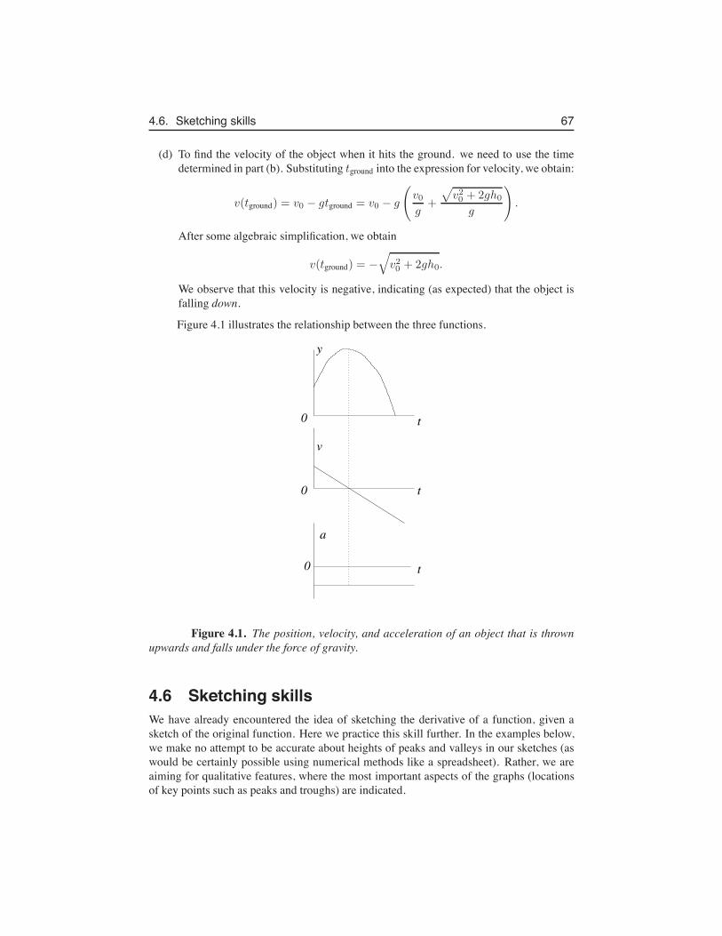
4.6. Sketching skills 67
(d) To find the velocity of the object when it hits the ground. we need to use the timedetermined in part (b). Substituting tground into the expression for velocity, we obtain:
v(tground) = v0 − gtground = v0 − g
(
v0g
+
√
v20 + 2gh0
g
)
.
After some algebraic simplification, we obtain
v(tground) = −√
v20 + 2gh0.
We observe that this velocity is negative, indicating (as expected) that the object isfalling down.
Figure 4.1 illustrates the relationship between the three functions.
t
t
t
y
v
a
0
0
0
Figure 4.1. The position, velocity, and acceleration of an object that is thrownupwards and falls under the force of gravity.
4.6 Sketching skillsWe have already encountered the idea of sketching the derivative of a function, given asketch of the original function. Here we practice this skill further. In the examples below,we make no attempt to be accurate about heights of peaks and valleys in our sketches (aswould be certainly possible using numerical methods like a spreadsheet). Rather, we areaiming for qualitative features, where the most important aspects of the graphs (locationsof key points such as peaks and troughs) are indicated.
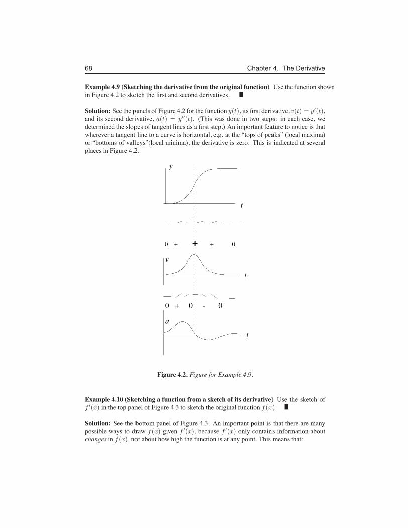
68 Chapter 4. The Derivative
Example 4.9 (Sketching the derivative from the original function) Use the function shownin Figure 4.2 to sketch the first and second derivatives.
Solution: See the panels of Figure 4.2 for the function y(t), its first derivative, v(t) = y′(t),and its second derivative, a(t) = y′′(t). (This was done in two steps: in each case, wedetermined the slopes of tangent lines as a first step.) An important feature to notice is thatwherever a tangent line to a curve is horizontal, e.g. at the “tops of peaks” (local maxima)or “bottoms of valleys”(local minima), the derivative is zero. This is indicated at severalplaces in Figure 4.2.
0 + + 0+
0 + 0 - 0
t
t
t
y
v
a
Figure 4.2. Figure for Example 4.9.
Example 4.10 (Sketching a function from a sketch of its derivative) Use the sketch off ′(x) in the top panel of Figure 4.3 to sketch the original function f(x)
Solution: See the bottom panel of Figure 4.3. An important point is that there are manypossible ways to draw f(x) given f ′(x), because f ′(x) only contains information aboutchanges in f(x), not about how high the function is at any point. This means that:
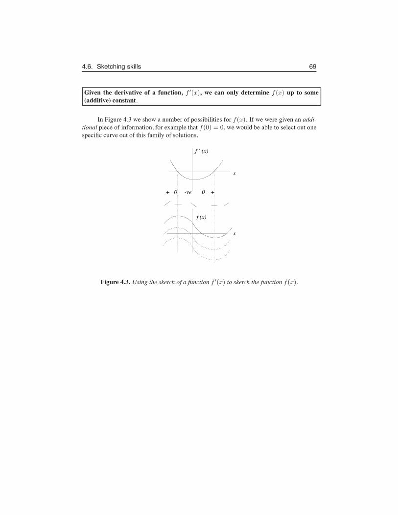
4.6. Sketching skills 69
Given the derivative of a function, f ′(x), we can only determine f(x) up to some(additive) constant.
In Figure 4.3 we show a number of possibilities for f(x). If we were given an addi-tional piece of information, for example that f(0) = 0, we would be able to select out onespecific curve out of this family of solutions.
+ 0 -ve 0 +
x
x
f ’ (x)
f (x)
Figure 4.3. Using the sketch of a function f ′(x) to sketch the function f(x).
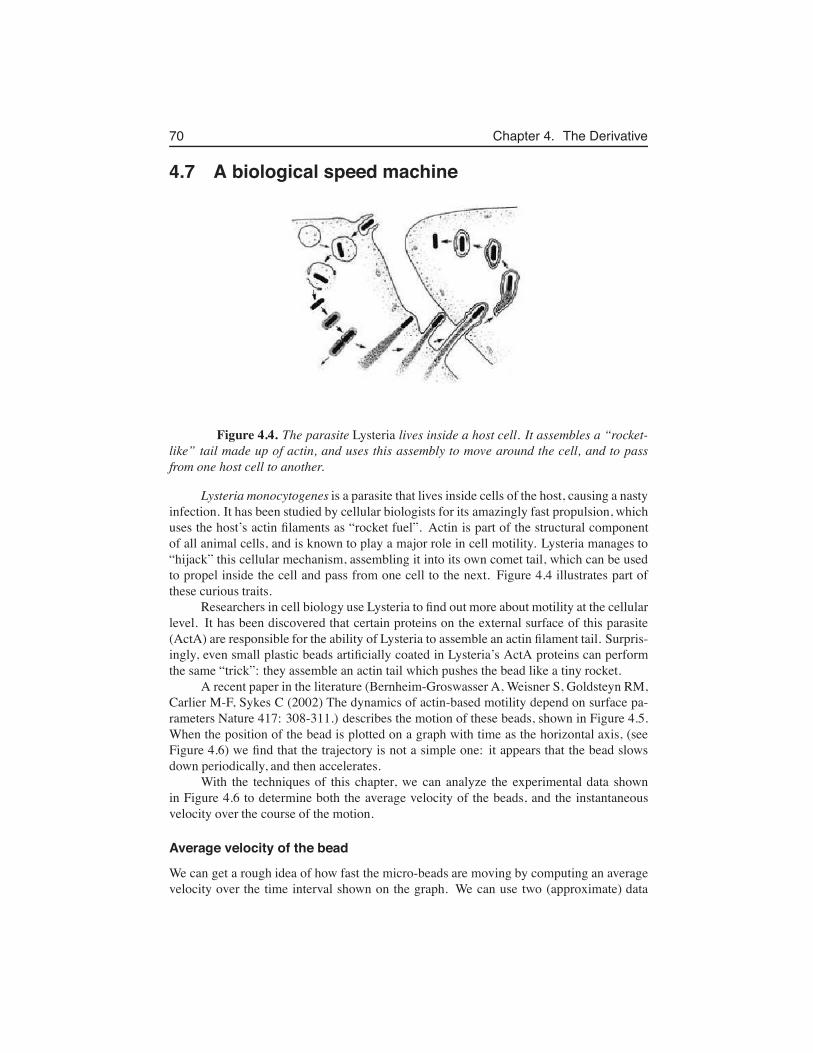
70 Chapter 4. The Derivative
4.7 A biological speed machine
Figure 4.4. The parasite Lysteria lives inside a host cell. It assembles a “rocket-like” tail made up of actin, and uses this assembly to move around the cell, and to passfrom one host cell to another.
Lysteria monocytogenes is a parasite that lives inside cells of the host, causing a nastyinfection. It has been studied by cellular biologists for its amazingly fast propulsion, whichuses the host’s actin filaments as “rocket fuel”. Actin is part of the structural componentof all animal cells, and is known to play a major role in cell motility. Lysteria manages to“hijack” this cellular mechanism, assembling it into its own comet tail, which can be usedto propel inside the cell and pass from one cell to the next. Figure 4.4 illustrates part ofthese curious traits.
Researchers in cell biology use Lysteria to find out more about motility at the cellularlevel. It has been discovered that certain proteins on the external surface of this parasite(ActA) are responsible for the ability of Lysteria to assemble an actin filament tail. Surpris-ingly, even small plastic beads artificially coated in Lysteria’s ActA proteins can performthe same “trick”: they assemble an actin tail which pushes the bead like a tiny rocket.
A recent paper in the literature (Bernheim-Groswasser A, Weisner S, Goldsteyn RM,Carlier M-F, Sykes C (2002) The dynamics of actin-based motility depend on surface pa-rameters Nature 417: 308-311.) describes the motion of these beads, shown in Figure 4.5.When the position of the bead is plotted on a graph with time as the horizontal axis, (seeFigure 4.6) we find that the trajectory is not a simple one: it appears that the bead slowsdown periodically, and then accelerates.
With the techniques of this chapter, we can analyze the experimental data shownin Figure 4.6 to determine both the average velocity of the beads, and the instantaneousvelocity over the course of the motion.
Average velocity of the bead
We can get a rough idea of how fast the micro-beads are moving by computing an averagevelocity over the time interval shown on the graph. We can use two (approximate) data
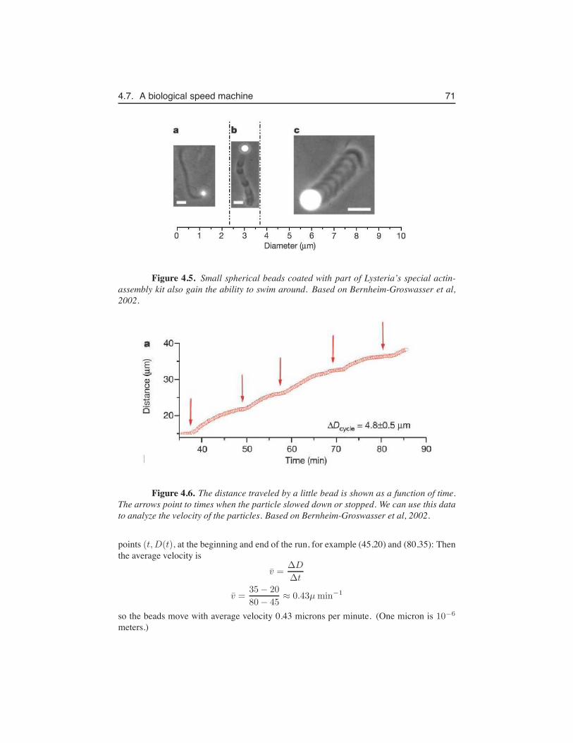
4.7. A biological speed machine 71
Figure 4.5. Small spherical beads coated with part of Lysteria’s special actin-assembly kit also gain the ability to swim around. Based on Bernheim-Groswasser et al,2002.
Figure 4.6. The distance traveled by a little bead is shown as a function of time.The arrows point to times when the particle slowed down or stopped. We can use this datato analyze the velocity of the particles. Based on Bernheim-Groswasser et al, 2002.
points (t,D(t), at the beginning and end of the run, for example (45,20) and (80,35): Thenthe average velocity is
v̄ =∆D
∆t
v̄ =35− 20
80− 45≈ 0.43µmin−1
so the beads move with average velocity 0.43 microns per minute. (One micron is 10−6
meters.)
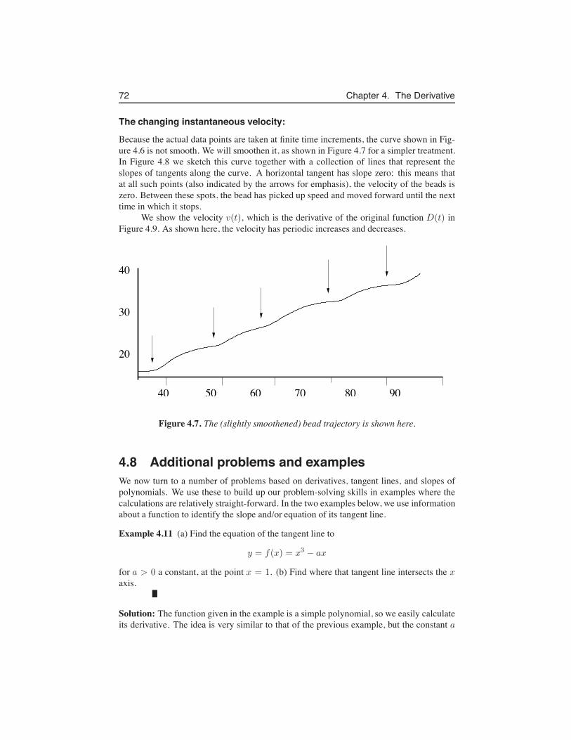
72 Chapter 4. The Derivative
The changing instantaneous velocity:
Because the actual data points are taken at finite time increments, the curve shown in Fig-ure 4.6 is not smooth. We will smoothen it, as shown in Figure 4.7 for a simpler treatment.In Figure 4.8 we sketch this curve together with a collection of lines that represent theslopes of tangents along the curve. A horizontal tangent has slope zero: this means thatat all such points (also indicated by the arrows for emphasis), the velocity of the beads iszero. Between these spots, the bead has picked up speed and moved forward until the nexttime in which it stops.
We show the velocity v(t), which is the derivative of the original function D(t) inFigure 4.9. As shown here, the velocity has periodic increases and decreases.
40 50 60 70 80 90
40
30
20
Figure 4.7. The (slightly smoothened) bead trajectory is shown here.
4.8 Additional problems and examplesWe now turn to a number of problems based on derivatives, tangent lines, and slopes ofpolynomials. We use these to build up our problem-solving skills in examples where thecalculations are relatively straight-forward. In the two examples below, we use informationabout a function to identify the slope and/or equation of its tangent line.
Example 4.11 (a) Find the equation of the tangent line to
y = f(x) = x3 − ax
for a > 0 a constant, at the point x = 1. (b) Find where that tangent line intersects the xaxis.
Solution: The function given in the example is a simple polynomial, so we easily calculateits derivative. The idea is very similar to that of the previous example, but the constant a
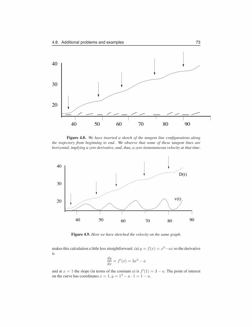
4.8. Additional problems and examples 73
40 50 60 70 80 90
40
30
20
Figure 4.8. We have inserted a sketch of the tangent line configurations alongthe trajectory from beginning to end. We observe that some of these tangent lines arehorizontal, implying a zero derivative, and, thus, a zero instantaneous velocity at that time.
40
30
20
D(t)
v(t)
40 50 60 70 9080
Figure 4.9. Here we have sketched the velocity on the same graph.
makes this calculation a little less straightforward. (a) y = f(x) = x3−ax so the derivativeis
dy
dx= f ′(x) = 3x2 − a
and at x = 1 the slope (in terms of the constant a) is f ′(1) = 3 − a. The point of intereston the curve has coordinates x = 1, y = 13 − a · 1 = 1− a.
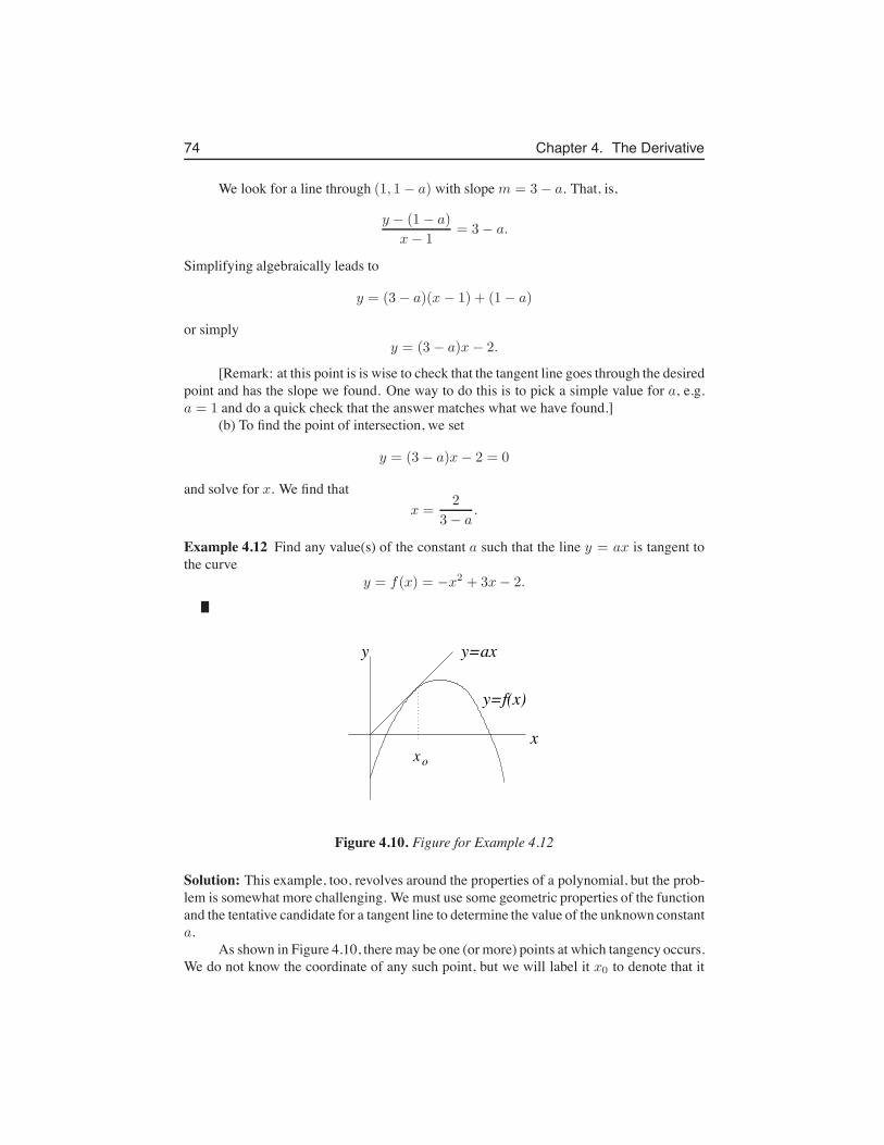
74 Chapter 4. The Derivative
We look for a line through (1, 1− a) with slope m = 3− a. That, is,
y − (1− a)
x− 1= 3− a.
Simplifying algebraically leads to
y = (3− a)(x − 1) + (1− a)
or simplyy = (3 − a)x− 2.
[Remark: at this point is is wise to check that the tangent line goes through the desiredpoint and has the slope we found. One way to do this is to pick a simple value for a, e.g.a = 1 and do a quick check that the answer matches what we have found.]
(b) To find the point of intersection, we set
y = (3− a)x− 2 = 0
and solve for x. We find thatx =
2
3− a.
Example 4.12 Find any value(s) of the constant a such that the line y = ax is tangent tothe curve
y = f(x) = −x2 + 3x− 2.
xx
y
o
y=f(x)
y=ax
Figure 4.10. Figure for Example 4.12
Solution: This example, too, revolves around the properties of a polynomial, but the prob-lem is somewhat more challenging. We must use some geometric properties of the functionand the tentative candidate for a tangent line to determine the value of the unknown constanta.
As shown in Figure 4.10, there may be one (or more) points at which tangency occurs.We do not know the coordinate of any such point, but we will label it x0 to denote that it
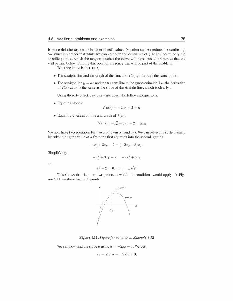
4.8. Additional problems and examples 75
is some definite (as yet to be determined) value. Notation can sometimes be confusing.We must remember that while we can compute the derivative of f at any point, only thespecific point at which the tangent touches the curve will have special properties that wewill outline below. Finding that point of tangency, x0, will be part of the problem.
What we know is that, at x0,
• The straight line and the graph of the function f(x) go through the same point.
• The straight line y = ax and the tangent line to the graph coincide, i.e. the derivativeof f(x) at x0 is the same as the slope of the straight line, which is clearly a
Using these two facts, we can write down the following equations:
• Equating slopes:f ′(x0) = −2x0 + 3 = a
• Equating y values on line and graph of f(x):
f(x0) = −x20 + 3x0 − 2 = ax0
We now have two equations for two unknowns, (a and x0). We can solve this system easilyby substituting the value of a from the first equation into the second, getting
−x20 + 3x0 − 2 = (−2x0 + 3)x0.
Simplifying:−x2
0 + 3x0 − 2 = −2x20 + 3x0
sox20 − 2 = 0, x0 = ±
√2.
This shows that there are two points at which the conditions would apply. In Fig-ure 4.11 we show two such points.
xx
y
o
y=f(x)
y=ax
Figure 4.11. Figure for solution to Example 4.12
We can now find the slope a using a = −2x0 + 3. We get:
x0 =√2 a = −2
√2 + 3,
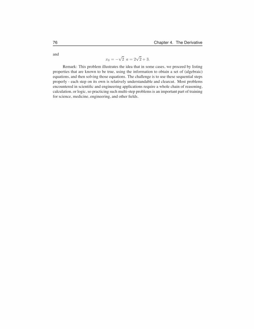
76 Chapter 4. The Derivative
andx0 = −
√2 a = 2
√2 + 3.
Remark: This problem illustrates the idea that in some cases, we proceed by listingproperties that are known to be true, using the information to obtain a set of (algebraic)equations, and then solving those equations. The challenge is to use these sequential stepsproperly - each step on its own is relatively understandable and clearcut. Most problemsencountered in scientific and engineering applications require a whole chain of reasoning,calculation, or logic, so practicing such multi-step problems is an important part of trainingfor science, medicine, engineering, and other fields.
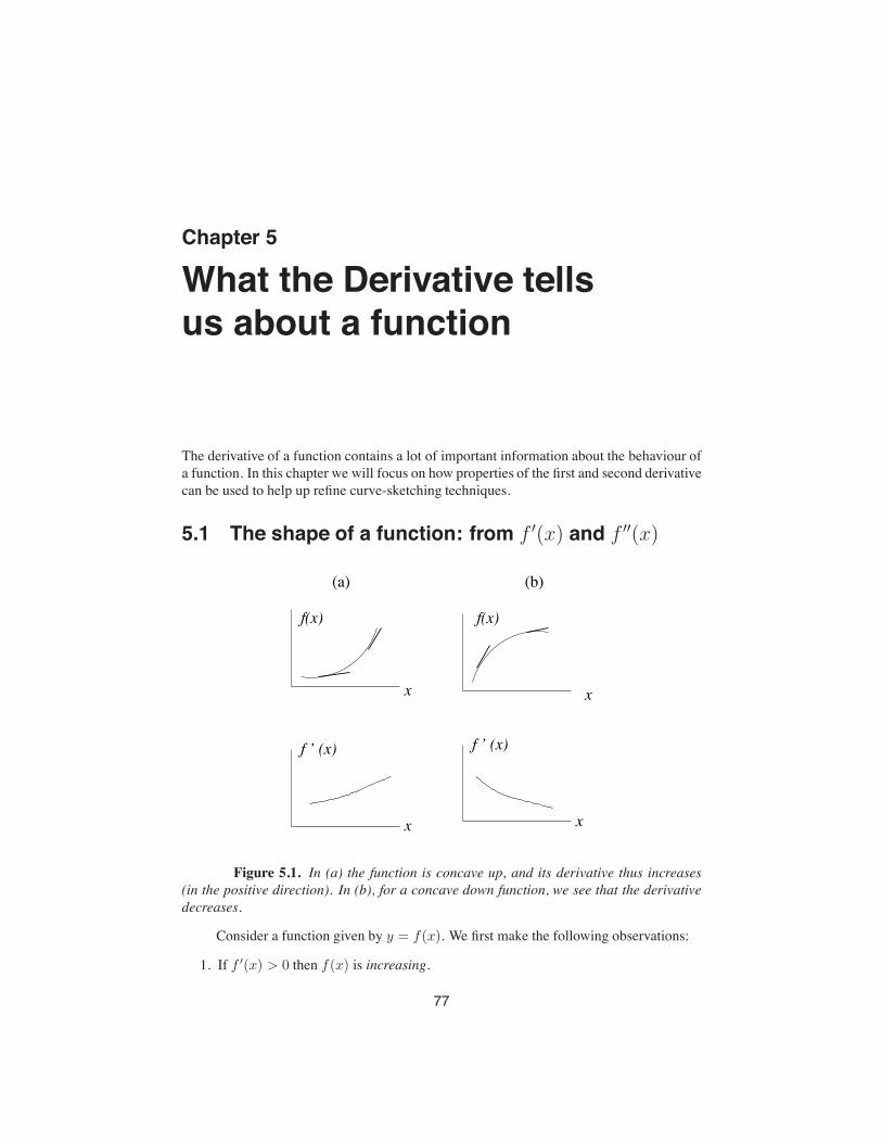
Chapter 5
What the Derivative tellsus about a function
The derivative of a function contains a lot of important information about the behaviour ofa function. In this chapter we will focus on how properties of the first and second derivativecan be used to help up refine curve-sketching techniques.
5.1 The shape of a function: from f ′(x) and f ′′(x)
x x
f(x) f(x)
(a) (b)
x x
f ’ (x) f ’ (x)
Figure 5.1. In (a) the function is concave up, and its derivative thus increases(in the positive direction). In (b), for a concave down function, we see that the derivativedecreases.
Consider a function given by y = f(x). We first make the following observations:
1. If f ′(x) > 0 then f(x) is increasing.
77
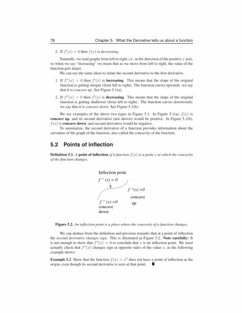
78 Chapter 5. What the Derivative tells us about a function
2. If f ′(x) < 0 then f(x) is decreasing.
Naturally, we read graphs from left to right, i.e. in the direction of the positive x axis,so when we say “increasing” we mean that as we move from left to right, the value of thefunction gets larger.
We can use the same ideas to relate the second derivative to the first derivative.
1. If f ′′(x) > 0 then f ′(x) is increasing. This means that the slope of the originalfunction is getting steeper (from left to right). The function curves upwards: we saythat it is concave up. See Figure 5.1(a).
2. If f ′′(x) < 0 then f ′(x) is decreasing. This means that the slope of the originalfunction is getting shallower (from left to right). The function curves downwards:we say that it is concave down. See Figure 5.1(b).
We see examples of the above two types in Figure 5.1. In Figure 5.1(a), f(x) isconcave up, and its second derivative (not shown) would be positive. In Figure 5.1(b),f(x) is concave down, and second derivative would be negative.
To summarize, the second derivative of a function provides information about thecurvature of the graph of the function, also called the concavity of the function.
5.2 Points of inflectionDefinition 5.1. A point of inflection of a function f(x) is a point x at which the concavityof the function changes.
f ’’(x) >0
f ’’ (x) <0
f ’’ (x) = 0
concaveup
concavedown
Inflection point
Figure 5.2. An inflection point is a place where the concavity of a function changes.
We can deduce from the definition and previous remarks that at a point of inflectionthe second derivative changes sign. This is illustrated in Figure 5.2. Note carefully: Itis not enough to show that f ′′(x) = 0 to conclude that x is an inflection point. We mustactually check that f ′′(x) changes sign at opposite sides of the value x, as the followingexample shows:
Example 5.2 Show that the function f(x) = x4 does not have a point of inflection at theorigin, even though its second derivative is zero at that point.
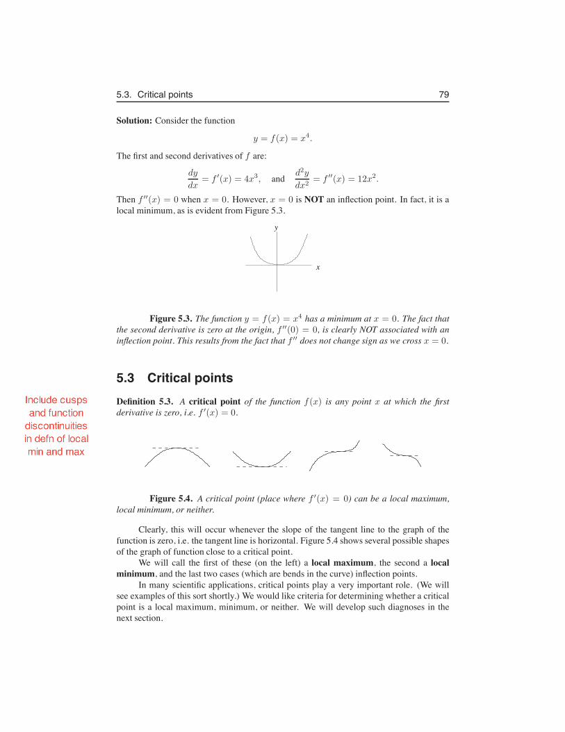
5.3. Critical points 79
Solution: Consider the function
y = f(x) = x4.
The first and second derivatives of f are:
dy
dx= f ′(x) = 4x3, and d2y
dx2= f ′′(x) = 12x2.
Then f ′′(x) = 0 when x = 0. However, x = 0 is NOT an inflection point. In fact, it is alocal minimum, as is evident from Figure 5.3.
x
y
Figure 5.3. The function y = f(x) = x4 has a minimum at x = 0. The fact thatthe second derivative is zero at the origin, f ′′(0) = 0, is clearly NOT associated with aninflection point. This results from the fact that f ′′ does not change sign as we cross x = 0.
5.3 Critical pointsDefinition 5.3. A critical point of the function f(x) is any point x at which the firstderivative is zero, i.e. f ′(x) = 0.
Figure 5.4. A critical point (place where f ′(x) = 0) can be a local maximum,local minimum, or neither.
Clearly, this will occur whenever the slope of the tangent line to the graph of thefunction is zero, i.e. the tangent line is horizontal. Figure 5.4 shows several possible shapesof the graph of function close to a critical point.
We will call the first of these (on the left) a local maximum, the second a localminimum, and the last two cases (which are bends in the curve) inflection points.
In many scientific applications, critical points play a very important role. (We willsee examples of this sort shortly.) We would like criteria for determining whether a criticalpoint is a local maximum, minimum, or neither. We will develop such diagnoses in thenext section.
Leah Keshet
Include cusps and function discontinuities in defn of local min and max
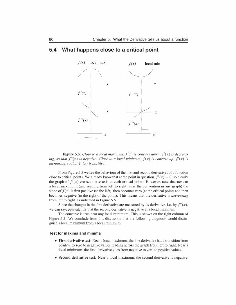
80 Chapter 5. What the Derivative tells us about a function
5.4 What happens close to a critical point
x x
x x
f (x) f (x)
f ’(x) f ’ (x)
x x
f ’’(x)f ’’(x)
local max local min
Figure 5.5. Close to a local maximum, f(x) is concave down, f ′(x) is decreas-ing, so that f ′′(x) is negative. Close to a local minimum, f(x) is concave up, f ′(x) isincreasing, so that f ′′(x) is positive.
From Figure 5.5 we see the behaviour of the first and second derivatives of a functionclose to critical points. We already know that at the point in question, f ′(x) = 0, so clearlythe graph of f ′(x) crosses the x axis at each critical point. However, note that next toa local maximum, (and reading from left to right, as is the convention in any graph) theslope of f(x) is first positive (to the left), then becomes zero (at the critical point) and thenbecomes negative (to the right of the point). This means that the derivative is decreasingfrom left to right, as indicated in Figure 5.5.
Since the changes in the first derivative are measured by its derivative, i.e. by f ′′(x),we can say, equivalently that the second derivative is negative at a local maximum.
The converse is true near any local minimum. This is shown on the right column ofFigure 5.5. We conclude from this discussion that the following diagnosis would distin-guish a local maximum from a local minimum:
Test for maxima and minima
• First derivative test: Near a local maximum, the first derivative has a transition frompositive to zero to negative values reading across the graph from left to right. Near alocal minimum, the first derivative goes from negative to zero to positive values.
• Second derivative test: Near a local maximum, the second derivative is negative.
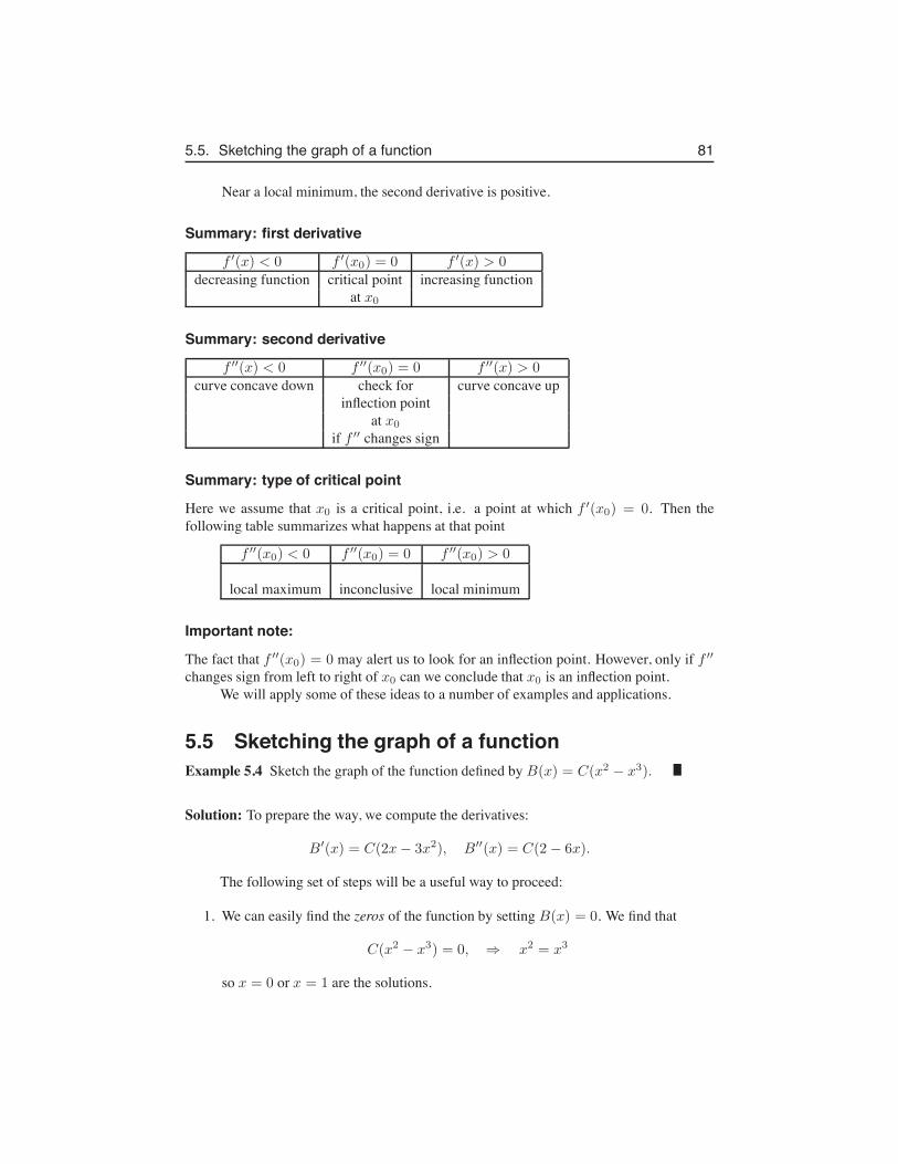
5.5. Sketching the graph of a function 81
Near a local minimum, the second derivative is positive.
Summary: first derivative
f ′(x) < 0 f ′(x0) = 0 f ′(x) > 0decreasing function critical point increasing function
at x0
Summary: second derivative
f ′′(x) < 0 f ′′(x0) = 0 f ′′(x) > 0curve concave down check for curve concave up
inflection pointat x0
if f ′′ changes sign
Summary: type of critical point
Here we assume that x0 is a critical point, i.e. a point at which f ′(x0) = 0. Then thefollowing table summarizes what happens at that point
f ′′(x0) < 0 f ′′(x0) = 0 f ′′(x0) > 0
local maximum inconclusive local minimum
Important note:
The fact that f ′′(x0) = 0 may alert us to look for an inflection point. However, only if f ′′
changes sign from left to right of x0 can we conclude that x0 is an inflection point.We will apply some of these ideas to a number of examples and applications.
5.5 Sketching the graph of a functionExample 5.4 Sketch the graph of the function defined by B(x) = C(x2 − x3).
Solution: To prepare the way, we compute the derivatives:
B′(x) = C(2x− 3x2), B′′(x) = C(2 − 6x).
The following set of steps will be a useful way to proceed:
1. We can easily find the zeros of the function by setting B(x) = 0. We find that
C(x2 − x3) = 0, ⇒ x2 = x3
so x = 0 or x = 1 are the solutions.
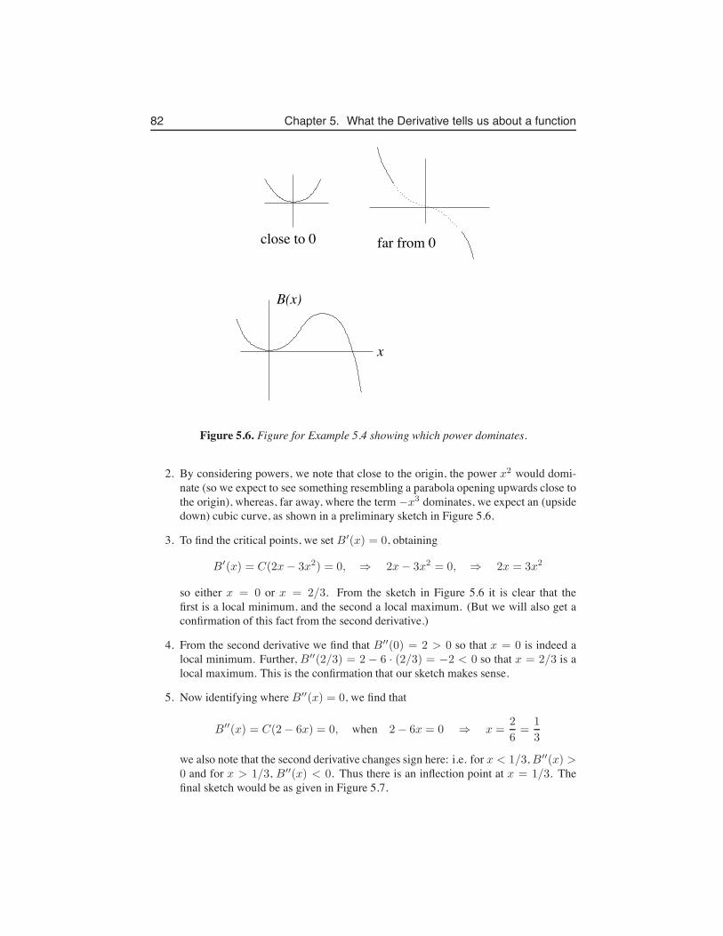
82 Chapter 5. What the Derivative tells us about a function
x
B(x)
close to 0 far from 0
Figure 5.6. Figure for Example 5.4 showing which power dominates.
2. By considering powers, we note that close to the origin, the power x2 would domi-nate (so we expect to see something resembling a parabola opening upwards close tothe origin), whereas, far away, where the term −x3 dominates, we expect an (upsidedown) cubic curve, as shown in a preliminary sketch in Figure 5.6.
3. To find the critical points, we set B′(x) = 0, obtaining
B′(x) = C(2x− 3x2) = 0, ⇒ 2x− 3x2 = 0, ⇒ 2x = 3x2
so either x = 0 or x = 2/3. From the sketch in Figure 5.6 it is clear that thefirst is a local minimum, and the second a local maximum. (But we will also get aconfirmation of this fact from the second derivative.)
4. From the second derivative we find that B′′(0) = 2 > 0 so that x = 0 is indeed alocal minimum. Further, B′′(2/3) = 2 − 6 · (2/3) = −2 < 0 so that x = 2/3 is alocal maximum. This is the confirmation that our sketch makes sense.
5. Now identifying where B′′(x) = 0, we find that
B′′(x) = C(2− 6x) = 0, when 2− 6x = 0 ⇒ x =2
6=
1
3
we also note that the second derivative changes sign here: i.e. for x < 1/3, B′′(x) >0 and for x > 1/3, B′′(x) < 0. Thus there is an inflection point at x = 1/3. Thefinal sketch would be as given in Figure 5.7.
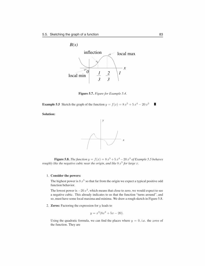
5.5. Sketching the graph of a function 83
x1 2 0 13 3
local max
local min
B(x)inflection
Figure 5.7. Figure for Example 5.4.
Example 5.5 Sketch the graph of the function y = f(x) = 8 x5 + 5 x4 − 20 x3
Solution:
x
y
Figure 5.8. The function y = f(x) = 8 x5+5 x4−20 x3 of Example 5.5 behavesroughly like the negative cubic near the origin, and like 8 x5 for large x.
1. Consider the powers:The highest power is 8 x5 so that far from the origin we expect a typical positive oddfunction behavior.The lowest power is −20 x3, which means that close to zero, we would expect to seea negative cubic. This already indicates to us that the function “turns around”, andso, must have some local maxima and minima. We draw a rough sketch in Figure 5.8.
2. Zeros: Factoring the expression for y leads to
y = x3(8x2 + 5x− 20).
Using the quadratic formula, we can find the places where y = 0, i.e. the zeros ofthe function. They are
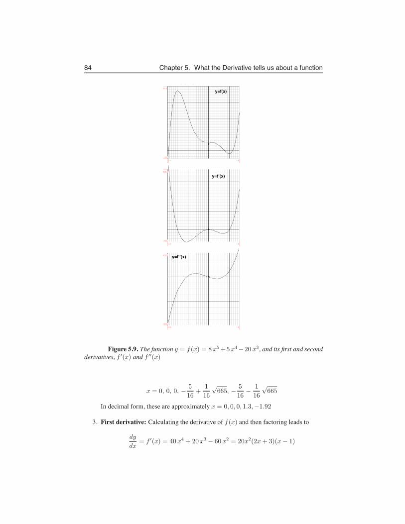
84 Chapter 5. What the Derivative tells us about a function
0
y=f(x)
-2.0 1.5-10.0
35.0
0
y=f’(x)
-2.0 1.5-40.0
200.0
0
y=f’’(x)
-2.0 1.5-800.0
400.0
Figure 5.9. The function y = f(x) = 8 x5+5 x4−20 x3, and its first and secondderivatives, f ′(x) and f ′′(x)
x = 0, 0, 0, −5
16+
1
16
√665, −
5
16−
1
16
√665
In decimal form, these are approximately x = 0, 0, 0, 1.3,−1.92
3. First derivative: Calculating the derivative of f(x) and then factoring leads to
dy
dx= f ′(x) = 40 x4 + 20 x3 − 60 x2 = 20x2(2x+ 3)(x− 1)
5.6. Product and Quotient rules for derivatives 85
so that the places where this derivative is zero are: x = 0, 0, 1,−3/2. We expectcritical points at these places.
4. Second derivative: We calculate the second derivative and factor to obtain
d2y
dx2= f ′′(x) = 160 x3 + 60 x2 − 120 x = 20x(8x2 + 3x− 6)
Thus, we can find places where the second derivative is zero. This occurs at
x = 0, −3
16+
1
16
√201, −
3
16−
1
16
√201
The values of these roots can be approximated by: x = 0, 0.69,−1.07
5. Classifying the critical points: To identify the types of critical points, we can usethe second derivative test, i.e. determine the sign of the second derivative at each ofthe critical points.
At x = 0 we see that f ′′(0) = 0 so the test is inconclusive. At x = 1, we havef ′′(1) = 20(8 + 3 − 6) > 0 implying that this is a local minimum. At x = −3/2we have f ′′(−1.5) = −225 < 0 so this is a local maximum. In fact we find that thevalue of the function at x = −1.5 is y = f(−1.5) = 32.0625, whereas at x = 1f(1) = −7.
The table below summarizes what we have found, and what we concluded. Each ofthe values of x across its top row has some significance in terms of the behaviour of thefunction.
x = −1.92 −1.5 −1.07 0 0.69 1 1.3f(x) = 0 32.0 0 −7 0f ′(x) = 0 0 0f ′′(x) = < 0 0 0 0 > 0
zero max inflection inflection min zero
We can now sketch the shape of the function, and its first and second derivatives inFigure 5.9.
5.6 Product and Quotient rules for derivativesSo far, using a single “rule” for differentiation, the power rule, together with properties ofthe derivative such as additivity and constant multiplication (described in Section 4.2), wewere able to calculate derivatives of polynomials. here we state without proof, two otherrules of differentiation that will prove to be useful in due time.
86 Chapter 5. What the Derivative tells us about a function
The product rule: If f(x) and g(x) are two functions, each differentiable in the domainof interest, then
d[f(x)g(x)]
dx=
df(x)
dxg(x) +
dg(x)
dxf(x).
Another notation for this rule is
[f(x)g(x)]′ = f ′(x)g(x) + g′(x)f(x).
Example 5.6 Find the derivative of the product of the two functions f(x) = x and g(x) =1 + x.
Solution: Using the product rule leads to
d[f(x)g(x)]
dx=
d[x(1 + x)]
dx=
d[x]
dx·(1+x)+
d[(1 + x)]
dx·x = 1 ·(1+x)+1 ·x = 2x+1.
(This can be easily checked by noting that f(x)g(x) = x(1+x) = x+x2, whose derivativeagrees with the above.)
The quotient rule: If f(x) and g(x) are two functions, each differentiable in the domainof interest, then
d
dx
[
f(x)
g(x)
]
=df(x)dx g(x)− dg(x)
dx f(x)
[g(x)]2.
We can also write this in the form[
f(x)
g(x)
]′
=f ′(x)g(x) − g′(x)f(x)
[g(x)]2.
Example 5.7 Find the derivative of the function y = ax−n = a/xn where a is a constantand n is a positive integer.
Solution: We can rewrite this as the quotient of the two functions f(x) = a and g(x) = xn.Then y = f(x)/g(x) so, using the quotient rule leads to the derivative
dy
dx=
f ′(x)g(x) − g′(x)f(x)
[g(x)]2=
0 · xn − (nxn−1) · a(xn)2
=−anxn−1
x2n
After algebraic simplification, we obtain dy/dx = a(−n)xn−1−2n = a(−n)x−n−1. Thisis an interesting result: The power rule of differentiation holds for negative integerpowers.
5.7. Global maxima and minima: behaviour at the endpoints of an interval 87
5.7 Global maxima and minima: behaviour at theendpoints of an interval
Global (absolute) maxima and minima:
A global (or absolute) maximum of a function y = f(x) over some interval is the largestvalue that the function attains on that interval. Similarly a global (or absolute) minimum isthe smallest value.
Comment: If the function is defined on a closed interval, we must check both thelocal maxima and minima as well as the endpoints of the interval to determine where theglobal maxima and minima occur.
Example 5.8 Consider the function y = f(x) = 2x + x2 0.1 < x < 4. Find the largest
and smallest values that this function takes over the given interval.
Solution: We first compute the derivatives:
f ′(x) = −21
x2+ 2x,
f ′′(x) = 41
x3+ 2.
We now determine where critical points f ′(x) = 0 occur:
−21
x2+ 2x = 0.
Simplifying, we find −2 1x2 = 2x, so x3 = 1 and the critical point is at x = 1. Observe that
the second derivative at this point is
f ′′(1) = 41
13+ 2 = 6 > 0,
so that x = 1 is a local minimum.We now calculate the value of the function at the endpoints x = 0.1 and x = 4
as well as at the critical point x = 1 to determine where global and local minima and/ormaxima occur:
f(0.1) = 20.01 f(1) = 3 f(4) = 16.5global maximum global minimum
We see that the global minimum occurs at x = 1. There are no local maxima. Theglobal maximum occurs at the left endpoint.
5.8 For further study: Automatic landing systemWe now discuss a practical example that uses many of the ideas so far. Our goal is to designan automatic landing system for an airplane.
We would like to find a polynomial of smallest degree that would describe the trajec-tory of an airplane as it makes its final approach to a landing site. We will assume that thelanding trajectory starts when the plane is at a distance x0 from the site where it touchesdown (at x = 0) and that it has been flying at a level (horizontal) direction up to that point.(See Figure 5.10.) We also want to make sure that the landing is as smooth as possible!
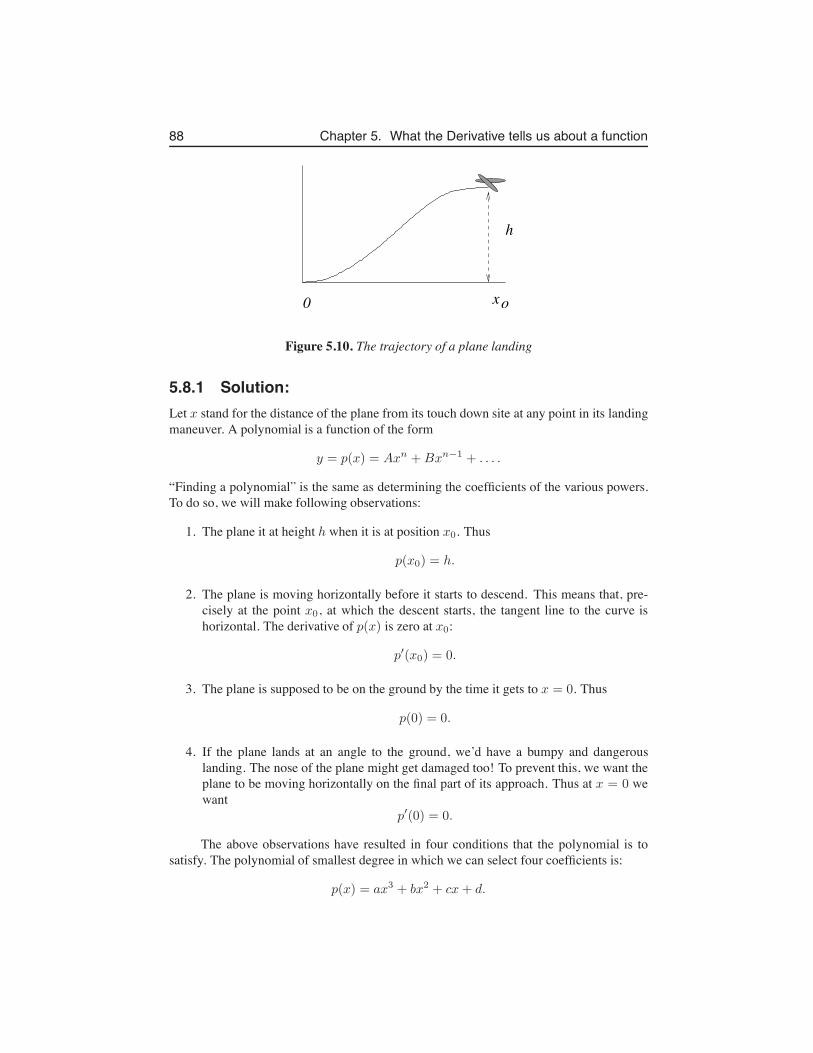
88 Chapter 5. What the Derivative tells us about a function
xo0
h
Figure 5.10. The trajectory of a plane landing
5.8.1 Solution:Let x stand for the distance of the plane from its touch down site at any point in its landingmaneuver. A polynomial is a function of the form
y = p(x) = Axn +Bxn−1 + . . . .
“Finding a polynomial” is the same as determining the coefficients of the various powers.To do so, we will make following observations:
1. The plane it at height h when it is at position x0. Thus
p(x0) = h.
2. The plane is moving horizontally before it starts to descend. This means that, pre-cisely at the point x0, at which the descent starts, the tangent line to the curve ishorizontal. The derivative of p(x) is zero at x0:
p′(x0) = 0.
3. The plane is supposed to be on the ground by the time it gets to x = 0. Thus
p(0) = 0.
4. If the plane lands at an angle to the ground, we’d have a bumpy and dangerouslanding. The nose of the plane might get damaged too! To prevent this, we want theplane to be moving horizontally on the final part of its approach. Thus at x = 0 wewant
p′(0) = 0.
The above observations have resulted in four conditions that the polynomial is tosatisfy. The polynomial of smallest degree in which we can select four coefficients is:
p(x) = ax3 + bx2 + cx+ d.
5.8. For further study: Automatic landing system 89
Below, we show how to solve for each of these coefficients in terms of the height h and thelocation x0 at which descent starts. (Note: if we use a polynomial of higher degree, ourfour conditions would not suffice to completely determine all the coefficients. Since we areasked to find the polynomial of least degree, we shall settle on this cubic polynomial.)
We will need to use the fact that the derivative of this polynomial is
p′(x) = 3ax2 + 2bx+ c.
From the above conditions we get:
1. p(x0) = h. Thusp(x0) = ax3
0 + bx20 + cx0 + d = h.
2. p′(x0) = 0. Thusp′(x0) = 3ax2
0 + 2bx0 + c = 0.
3. p(0) = 0. Thusp(0) = a · 03 + b · 02 + c · 0 + d = 0.
All the terms disappear but one, from which we conclude that d = 0.
4. p′(0) = 0. Thusp′(0) = 3a · 02 + 2b · 0 + c = 0.
Again, all terms but one disappear, leaving c = 0.
Using the fact that c, d = 0, and returning to the first two equations, we are left withtwo equations and two unknowns:
ax30 + bx2
0 = h,
3ax20 + 2bx0 = 0
(Remember that here we are trying to find the values of the unknown coefficients a, b, andthe quantities x0 and h are known fixed constants that represent the starting point of theplane as it initiates landing procedures.)
Solving for a and b we get, from the second equation:
3ax20 = −2bx0, a = −
2b
3x0.
Plugging into the first we arrive at:
−2b
3x0x30 + bx2
0 = h
−2b
3x20 + bx2
0 = h
bx20
(
−2
3+ 1
)
= h
90 Chapter 5. What the Derivative tells us about a function
so, after simplification, we get
b =3h
x20
, a = −2b
3x0= −
2h
x30
.
Thus, we have arrived at the desired result:
p(x) =
(
−2h
x30
)
x3 +
(
3h
x20
)
x2.
(The expression looks cumbersome, but we remember that the terms in brackets are actuallyconstants.)
To illustrate how this would work in a specific example, suppose that the plane startsits descent 20 km away from the airport at a height of 1 km. Then x0 = 20, h = 1, so
b =3
202= 0.0075, a = −
2
203= −0.00025.
In this case, the polynomial that describes the landing trajectory would be:
p(x) = −0.00025x3 + 0.0075x2
Exercises 91
Exercises5.1. A zero of a function is a place where f(x) = 0.
(a) Find the zeros, local maxima, and minima of the polynomial y = f(x) =x3 − 3x
(b) Find the local minima and maxima of the polynomial y = f(x) = (2/3)x3 −3x2 + 4x.
(c) A point of inflection is a point at which the second derivative changes sign.Determine whether each of the polynomials given in parts (a) and (b) have aninflection point.
5.2. Find the absolute maximum and minimum values on the given interval:(a) y = 2x2 on −3 ≤ x ≤ 3
(b) y = (x − 5)2 on 0 ≤ x ≤ 6
(c) y = x2 − x− 6 on 1 ≤ x ≤ 3
(d) y =1
x+ x on −4 ≤ x ≤ −
1
2.
5.3. Sketch the graph of x4 − x2 + 1 in the range −3 to 3. Find its minimum value.5.4. Identify all the critical points of the following function.
y = x3 − 27
5.5. Consider the function g(x) = x4 − 2x3 + x2. Determine locations of critical pointsand inflection points.
5.6. Consider the polynomial y = x3 + 3x2 + ax + 1. Show that when a > 3 thispolynomial has no critical points.
5.7. Find the values of a, b, and c if the parabola y = ax2 + bx+ c is tangent to the liney = −2x+ 3 at (2,−1) and has a critical point when x = 3.
5.8. The position of a particle is given by the function y = f(t) = t3 + 3t2.(a) Find the velocity and the acceleration of the particle.(b) A second particle has position given by the function y = g(t) = at4 + t3
where a is some constant and a > 0. At what time(s) are the particles in thesame position?
(c) At what times do the particles have the same velocity?(d) When do the particles have the same acceleration?
5.9. Double Wells and Physics: In physics, a function such as
f(x) = x4 − 2x2
is often called a double well potential. Physicists like to think of this as a “land-scape” with hills and valleys. They imagine a ball rolling along such a landscape:with friction, the ball eventually comes to rest at the bottom of one of the valleysin this potential. Sketch a picture of this landscape and use information about thederivative of this function to predict where the ball might be found, i.e. where thevalley bottoms are located.
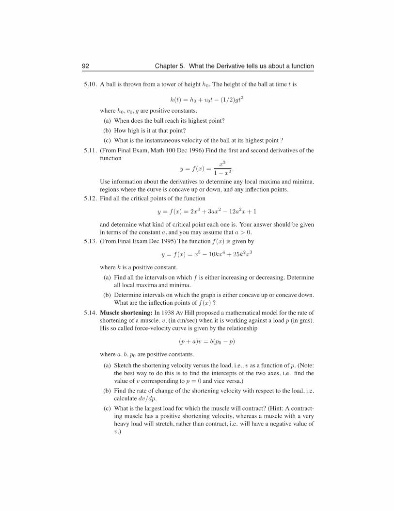
92 Chapter 5. What the Derivative tells us about a function
5.10. A ball is thrown from a tower of height h0. The height of the ball at time t is
h(t) = h0 + v0t− (1/2)gt2
where h0, v0, g are positive constants.(a) When does the ball reach its highest point?(b) How high is it at that point?(c) What is the instantaneous velocity of the ball at its highest point ?
5.11. (From Final Exam, Math 100 Dec 1996) Find the first and second derivatives of thefunction
y = f(x) =x3
1− x2.
Use information about the derivatives to determine any local maxima and minima,regions where the curve is concave up or down, and any inflection points.
5.12. Find all the critical points of the function
y = f(x) = 2x3 + 3ax2 − 12a2x+ 1
and determine what kind of critical point each one is. Your answer should be givenin terms of the constant a, and you may assume that a > 0.
5.13. (From Final Exam Dec 1995) The function f(x) is given by
y = f(x) = x5 − 10kx4 + 25k2x3
where k is a positive constant.(a) Find all the intervals on which f is either increasing or decreasing. Determine
all local maxima and minima.(b) Determine intervals on which the graph is either concave up or concave down.
What are the inflection points of f(x) ?5.14. Muscle shortening: In 1938 Av Hill proposed a mathematical model for the rate of
shortening of a muscle, v, (in cm/sec) when it is working against a load p (in gms).His so called force-velocity curve is given by the relationship
(p+ a)v = b(p0 − p)
where a, b, p0 are positive constants.
(a) Sketch the shortening velocity versus the load, i.e., v as a function of p. (Note:the best way to do this is to find the intercepts of the two axes, i.e. find thevalue of v corresponding to p = 0 and vice versa.)
(b) Find the rate of change of the shortening velocity with respect to the load, i.e.calculate dv/dp.
(c) What is the largest load for which the muscle will contract? (Hint: A contract-ing muscle has a positive shortening velocity, whereas a muscle with a veryheavy load will stretch, rather than contract, i.e. will have a negative value ofv.)
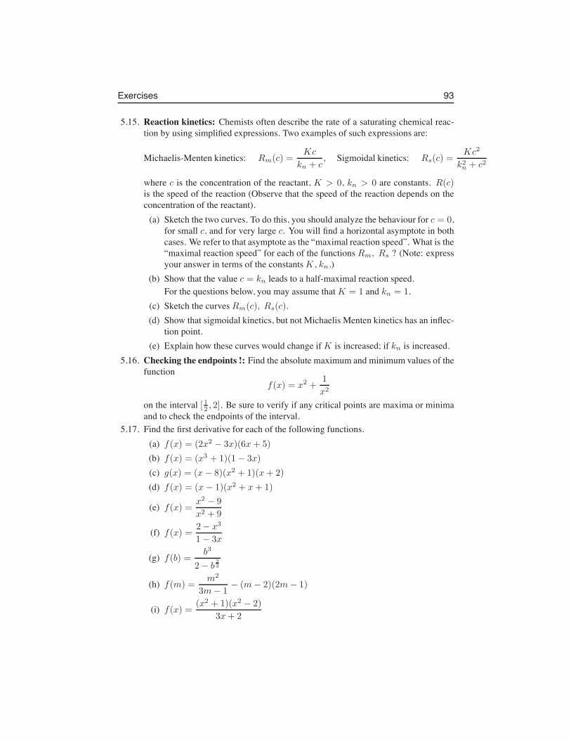
Exercises 93
5.15. Reaction kinetics: Chemists often describe the rate of a saturating chemical reac-tion by using simplified expressions. Two examples of such expressions are:
Michaelis-Menten kinetics: Rm(c) =Kc
kn + c, Sigmoidal kinetics: Rs(c) =
Kc2
k2n + c2
where c is the concentration of the reactant, K > 0, kn > 0 are constants. R(c)is the speed of the reaction (Observe that the speed of the reaction depends on theconcentration of the reactant).
(a) Sketch the two curves. To do this, you should analyze the behaviour for c = 0,for small c, and for very large c. You will find a horizontal asymptote in bothcases. We refer to that asymptote as the “maximal reaction speed”. What is the“maximal reaction speed” for each of the functions Rm, Rs ? (Note: expressyour answer in terms of the constants K , kn.)
(b) Show that the value c = kn leads to a half-maximal reaction speed.For the questions below, you may assume that K = 1 and kn = 1.
(c) Sketch the curves Rm(c), Rs(c).(d) Show that sigmoidal kinetics, but not Michaelis Menten kinetics has an inflec-
tion point.(e) Explain how these curves would change if K is increased; if kn is increased.
5.16. Checking the endpoints !: Find the absolute maximum and minimum values of thefunction
f(x) = x2 +1
x2
on the interval [ 12 , 2]. Be sure to verify if any critical points are maxima or minimaand to check the endpoints of the interval.
5.17. Find the first derivative for each of the following functions.(a) f(x) = (2x2 − 3x)(6x+ 5)
(b) f(x) = (x3 + 1)(1− 3x)
(c) g(x) = (x − 8)(x2 + 1)(x+ 2)
(d) f(x) = (x − 1)(x2 + x+ 1)
(e) f(x) =x2 − 9
x2 + 9
(f) f(x) =2− x3
1− 3x
(g) f(b) =b3
2− b23
(h) f(m) =m2
3m− 1− (m− 2)(2m− 1)
(i) f(x) =(x2 + 1)(x2 − 2)
3x+ 2

94 Chapter 5. What the Derivative tells us about a function
Chapter 6
Optimization
In this chapter, we collect a variety of problems in which the ideas developed in earliermaterial are put to use. In particular, we will use calculus to find local (and global) maxima,and minima so as to get the best (optimal) values of some desirable quantity. Setting upthese problems, from first verbal description, to clear cut mathematical formulation is themain challenge we will face. Often, we will use geometric ideas to express relationshipsbetween variables leading to our solution.
6.1 Density dependent (logistic) growth in apopulation
Biologists often notice that the growth rate of a population depends not only on the sizeof the population, but also on how crowded it is. When individuals have to compete forresources, nesting sites, mates, or food, they cannot reproduce as quickly, leading to adecline in the rate of growth of the population.
The rule that governs this growth, called logistic growth assumes that the growthrate G depends on the density of the population N as follows:
G(N) = rN
(
K −N
K
)
where r > 0 is a constant, called the intrinsic growth rate and K > 0 is a constant calledthe carrying capacity of the environment for the population. We will soon see that thelargest population that would grow at all is N = K . We show a sketch of this function inFigure 6.1. But how would we arrive at such a sketch?
Example 6.1 (Logistic growth rate:) Answer the following questions:
• Find the population density that leads to the maximal growth rate.
• What is the maximal growth rate?
• For what population size is the growth rate zero?
95
Leah Keshet
Leah Keshet
not a bounded interval
96 Chapter 6. Optimization
Solution:G(N) = rN
(
K −N
K
)
= rN −r
KN2
To find the maximal growth rate we differentiate G with respect to the variable N ,remembering that K, r > 0 are here treated as constants. We get
G′(N) = r − 2r
KN.
Setting G′(N) = 0 and solving for N leads to
r = 2r
KN ⇒ N =
K
2.
By taking a second derivative we find that
G′′(N) = −2r
K
which is negative for all population sizes. This tells us that the function G(N) is concavedown, and that N = K/2 is a local maximum. Thus the density leading to largest growthrate is one half of the carrying capacity.
The growth rate at this density is
G(K
2) = r
(
K
2
)
(
K − K2
K
)
= rK
2
1
2=
rK
4.
To find the population size at which the growth rate is zero, we set G = 0 and solve for N :
G(N) = rN
(
K −N
K
)
= 0.
The two solutions are N = 0 (which is not very interesting, since when there is no popula-tion there is no growth) and N = K .
We will have many more things to say about this type of density dependent growth alittle later on in this course.
6.2 Cell size and shapeWe have seen in Section 1.3 that the absorption and consumption rates A(r), C(r) for asimple spherical cell of radius r are:
A(r) = k1S = 4k1πr2, C(r) = k2V =
4
3πk2r
3,
where k1, k2 > 0 are constants and r is the radius of the cell. Here we examine the net rateof increase of nutrients, which is just the rate of absorption minus the rate of consumption.
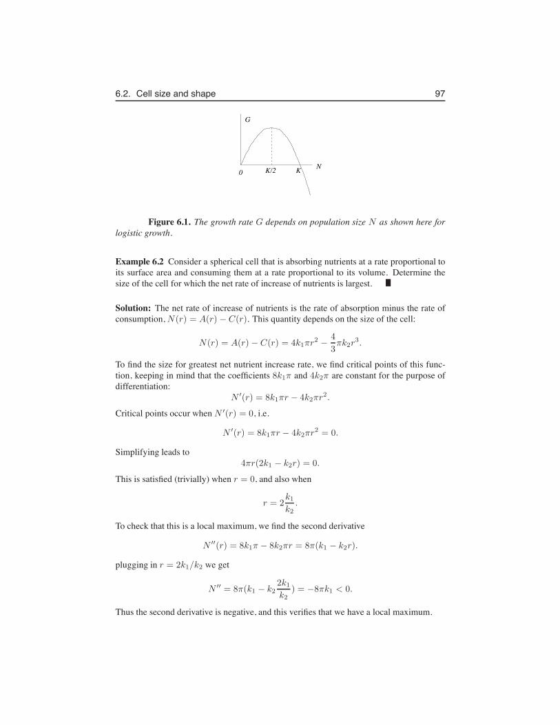
6.2. Cell size and shape 97
NK/2 K0
G
Figure 6.1. The growth rate G depends on population size N as shown here forlogistic growth.
Example 6.2 Consider a spherical cell that is absorbing nutrients at a rate proportional toits surface area and consuming them at a rate proportional to its volume. Determine thesize of the cell for which the net rate of increase of nutrients is largest.
Solution: The net rate of increase of nutrients is the rate of absorption minus the rate ofconsumption, N(r) = A(r) − C(r). This quantity depends on the size of the cell:
N(r) = A(r) − C(r) = 4k1πr2 −
4
3πk2r
3.
To find the size for greatest net nutrient increase rate, we find critical points of this func-tion, keeping in mind that the coefficients 8k1π and 4k2π are constant for the purpose ofdifferentiation:
N ′(r) = 8k1πr − 4k2πr2.
Critical points occur when N ′(r) = 0, i.e.
N ′(r) = 8k1πr − 4k2πr2 = 0.
Simplifying leads to4πr(2k1 − k2r) = 0.
This is satisfied (trivially) when r = 0, and also when
r = 2k1k2
.
To check that this is a local maximum, we find the second derivative
N ′′(r) = 8k1π − 8k2πr = 8π(k1 − k2r).
plugging in r = 2k1/k2 we get
N ′′ = 8π(k1 − k22k1k2
) = −8πk1 < 0.
Thus the second derivative is negative, and this verifies that we have a local maximum.
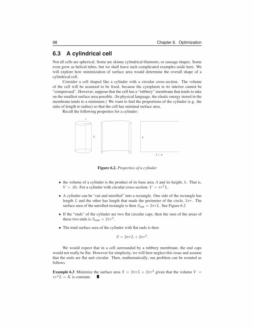
98 Chapter 6. Optimization
6.3 A cylindrical cellNot all cells are spherical. Some are skinny cylindrical filaments, or sausage shapes. Someeven grow as helical tubes, but we shall leave such complicated examples aside here. Wewill explore how minimization of surface area would determine the overall shape of acylindrical cell.
Consider a cell shaped like a cylinder with a circular cross-section. The volumeof the cell will be assumed to be fixed, because the cytoplasm in its interior cannot be“compressed”. However, suppose that the cell has a “rubbery” membrane that tends to takeon the smallest surface area possible. (In physical language, the elastic energy stored in themembrane tends to a minimum.) We want to find the proportions of the cylinder (e.g. theratio of length to radius) so that the cell has minimal surface area.
Recall the following properties for a cylinder:
2 r
L
r
L
!
Figure 6.2. Properties of a cylinder
• the volume of a cylinder is the product of its base area A and its height, h. That is,V = Ah. For a cylinder with circular cross-section: V = πr2L.
• A cylinder can be “cut and unrolled” into a rectangle. One side of the rectangle haslength L and the other has length that made the perimeter of the circle, 2πr. Thesurface area of the unrolled rectangle is then Sside = 2πrL. See Figure 6.2
• If the “ends” of the cylinder are two flat circular caps, then the sum of the areas ofthese two ends is Sends = 2πr2.
• The total surface area of the cylinder with flat ends is then
S = 2πrL+ 2πr2.
We would expect that in a cell surrounded by a rubbery membrane, the end capswould not really be flat. However for simplicity, we will here neglect this issue and assumethat the ends are flat and circular. Then, mathematically, our problem can be restated asfollows
Example 6.3 Minimize the surface area S = 2πrL + 2πr2 given that the volume V =πr2L = K is constant.
6.3. A cylindrical cell 99
Solution: The shape of the cell depends on both the length L, and the radius r of thecylinder. However, these are not independent . They are related to one another becausethe volume of the cell has to be constant. This is an example of an optimization problemwith a constraint, i.e. a condition that has to be satisfied. The constraint will allow us toeliminate one of the variables, as we show below.
The constraint is “the volume is fixed”, i.e.,
V = πr2L = K
where K > 0 is a constant that represents the volume of the given cell. We can use this toexpress one variable in terms of the other. For example, we can solve for L.
L =K
πr2. (6.1)
The function to minimize isS = 2πrL + 2πr2.
We eliminate L by using the previous relationship, (6.1) to obtain S as a function of ralone:
S(r) = 2πrK
πr2+ 2πr2
Simplification leads to
S(r) = 2K
r+ 2πr2.
observe that S is now clearly a function of the single variable, r, (K and π are constants).In order to find local minima, we will look for critical points of the function S(r).
We compute the relevant derivatives:
S′(r) = −2K
r2+ 4πr,
The second derivative will also be useful.
S′′(r) = 4K
r3+ 4π.
From the last calculation, we observe that the second derivative is always positive sinceK, r > 0, so the function S(r) is concave up. Any critical point we find thus will be aminimum automatically.
To find a critical point, set S′(r) = 0:
S′(r) = −2K
r2+ 4πr = 0.
Solving for r:
2K
r2= 4πr ⇒ r3 =
K
2π⇒ r =
(
K
2π
)1/3
.
100 Chapter 6. Optimization
We also find the length of this cell using Eqn. 6.1.
L =
(
4K
π
)1/3
.
This comes about from a manipulation of powers:
L =K
πr2= Kπ−1
(
K
2π
)−2/3
= K1−2/3π−1+2/322/3 = K1/3 π−1/3 41/3.
We can finally characterize the shape of the cell. One way to do this is to specify the ratio ofits radius to its length. Based on our previous results, we can compute that ratio as follows:
L
r=
(4K/π)1/3
(K/2π)1/3= 81/3 = 2.
Thus, the length of this cylinder is the same as its diameter (which is twice the radius). Thismeans that in a cylindrical cell with a rubbery membrane, we find a short and fat shape. Inorder for the cell to grow as a long skinny cylinder, it has to have some structural supportthat prevents the surface area from contracting to the smallest possible area. An example ofthis type occurs in fungal cells. These grow as long branched filaments. The outer cell wallcontains structural components that prevent the cell surface from contracting elastically.
I would like to thank Prof Nima Geffen (Tel Aviv University) with providing the inspi-ration for this example.
6.4 Geometric optimizationWe consider several other examples of optimization where volumes, lengths, and/or surfaceareas are considered.
Example 6.4 (Wrapping a rectangular box:) A box with square base and arbitrary heighthas string tied around each of its perimeter. The total length of string so used is 10 inches.Find the dimensions of the box with largest surface area. (That is, figure out what is thelargest amount of wrapping paper needed to wrap this box.)
Solution: The total length of string shown in Figure 6.3, consisting of three perimeters ofthe box is as follows:
L = 2(x+ x) + 2(x+ y) + 2(x+ y) = 8x+ 4y = 10.
This total length is to be kept constant, so the above equation is the constraint in thisproblem. This means that x and y are related to one another. We will use this fact toeliminate one of them from the formula for surface area.
The surface area of the box is
S = 4(xy) + 2x2.
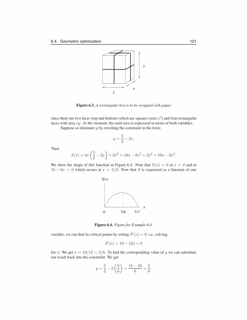
6.4. Geometric optimization 101
xx
y
Figure 6.3. A rectangular box is to be wrapped with paper
since there are two faces (top and bottom) which are squares (area x2) and four rectangularfaces with area xy. At the moment, the total area is expressed in terms of both variables.
Suppose se eliminate y by rewriting the constraint in the form:
y =5
2− 2x.
ThenS(x) = 4x
(
5
2− 2x
)
+ 2x2 = 10x− 8x2 + 2x2 = 10x− 6x2.
We show the shape of this function in Figure 6.4. Note that S(x) = 0 at x = 0 and at10 − 6x = 0 which occurs at x = 5/3. Now that S is expressed as a function of one
S(x)
x0 5/6 5/3
Figure 6.4. Figure for Example 6.4.
variable, we can find its critical points by setting S′(x) = 0, i.e., solving
S′(x) = 10− 12x = 0
for x: We get x = 10/12 = 5/6. To find the corresponding value of y we can substituteour result back into the constraint. We get
y =5
2− 2
(
5
6
)
=15− 10
6=
5
6.
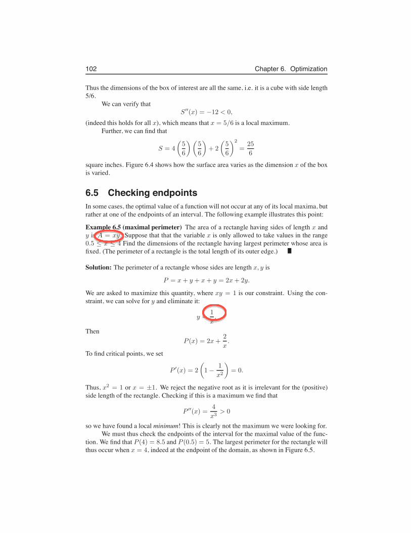
102 Chapter 6. Optimization
Thus the dimensions of the box of interest are all the same, i.e. it is a cube with side length5/6.
We can verify thatS′′(x) = −12 < 0,
(indeed this holds for all x), which means that x = 5/6 is a local maximum.Further, we can find that
S = 4
(
5
6
)(
5
6
)
+ 2
(
5
6
)2
=25
6
square inches. Figure 6.4 shows how the surface area varies as the dimension x of the boxis varied.
6.5 Checking endpointsIn some cases, the optimal value of a function will not occur at any of its local maxima, butrather at one of the endpoints of an interval. The following example illustrates this point:
Example 6.5 (maximal perimeter) The area of a rectangle having sides of length x andy is A = xy. Suppose that that the variable x is only allowed to take values in the range0.5 ≤ x ≤ 4 Find the dimensions of the rectangle having largest perimeter whose area isfixed. (The perimeter of a rectangle is the total length of its outer edge.)
Solution: The perimeter of a rectangle whose sides are length x, y is
P = x+ y + x+ y = 2x+ 2y.
We are asked to maximize this quantity, where xy = 1 is our constraint. Using the con-straint, we can solve for y and eliminate it:
y =1
x.
ThenP (x) = 2x+
2
x.
To find critical points, we set
P ′(x) = 2
(
1−1
x2
)
= 0.
Thus, x2 = 1 or x = ±1. We reject the negative root as it is irrelevant for the (positive)side length of the rectangle. Checking if this is a maximum we find that
P ′′(x) =4
x3> 0
so we have found a local minimum! This is clearly not the maximum we were looking for.We must thus check the endpoints of the interval for the maximal value of the func-
tion. We find that P (4) = 8.5 and P (0.5) = 5. The largest perimeter for the rectangle willthus occur when x = 4, indeed at the endpoint of the domain, as shown in Figure 6.5.
Leah Keshet
Leah Keshet
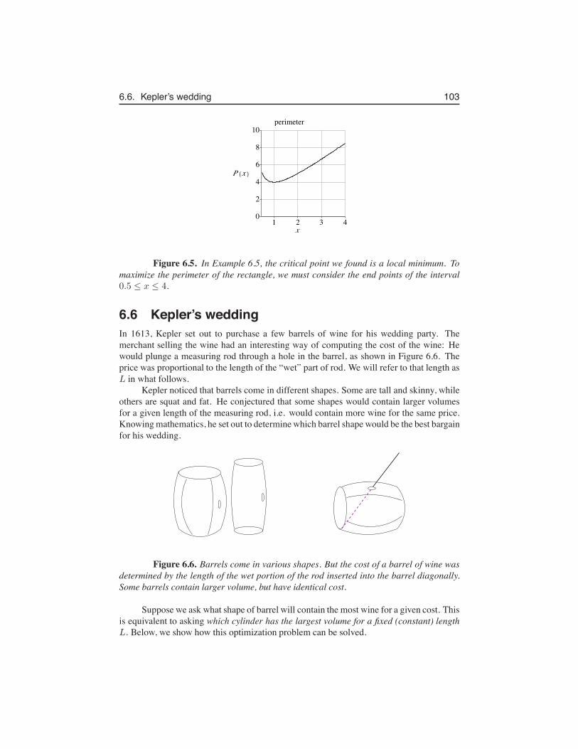
6.6. Kepler’s wedding 103
Figure 6.5. In Example 6.5, the critical point we found is a local minimum. Tomaximize the perimeter of the rectangle, we must consider the end points of the interval0.5 ≤ x ≤ 4.
6.6 Kepler’s weddingIn 1613, Kepler set out to purchase a few barrels of wine for his wedding party. Themerchant selling the wine had an interesting way of computing the cost of the wine: Hewould plunge a measuring rod through a hole in the barrel, as shown in Figure 6.6. Theprice was proportional to the length of the “wet” part of rod. We will refer to that length asL in what follows.
Kepler noticed that barrels come in different shapes. Some are tall and skinny, whileothers are squat and fat. He conjectured that some shapes would contain larger volumesfor a given length of the measuring rod, i.e. would contain more wine for the same price.Knowing mathematics, he set out to determine which barrel shape would be the best bargainfor his wedding.
Figure 6.6. Barrels come in various shapes. But the cost of a barrel of wine wasdetermined by the length of the wet portion of the rod inserted into the barrel diagonally.Some barrels contain larger volume, but have identical cost.
Suppose we ask what shape of barrel will contain the most wine for a given cost. Thisis equivalent to asking which cylinder has the largest volume for a fixed (constant) lengthL. Below, we show how this optimization problem can be solved.
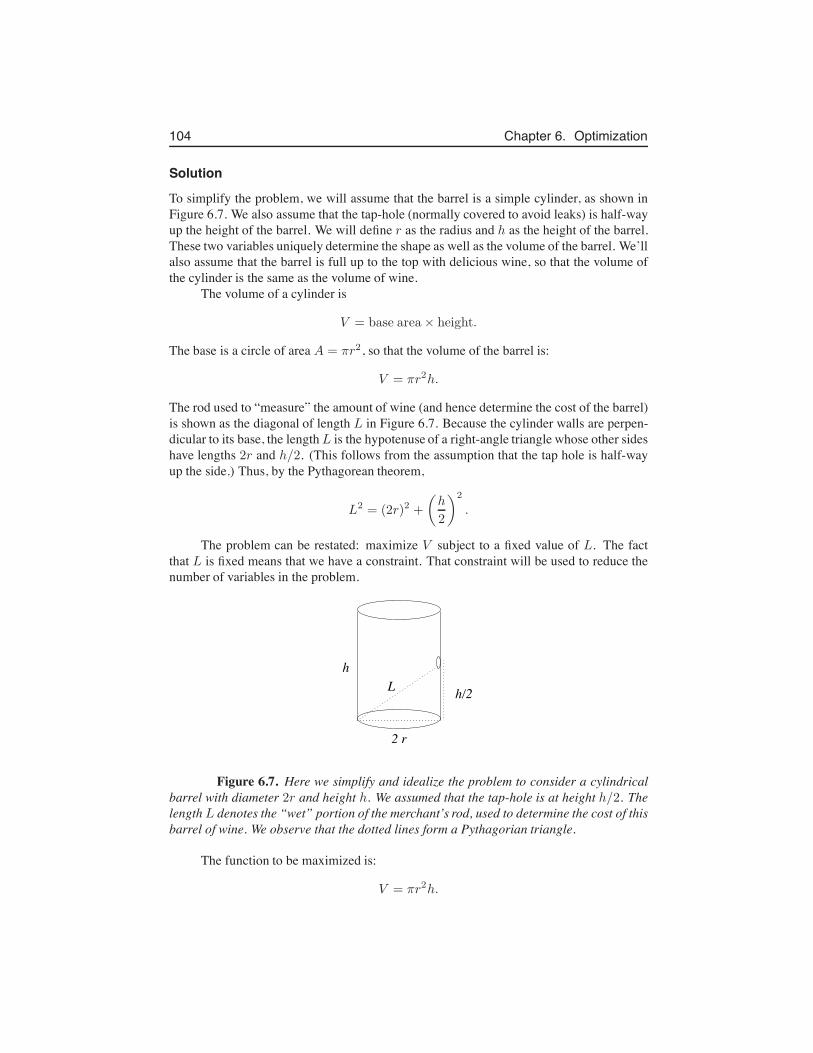
104 Chapter 6. Optimization
Solution
To simplify the problem, we will assume that the barrel is a simple cylinder, as shown inFigure 6.7. We also assume that the tap-hole (normally covered to avoid leaks) is half-wayup the height of the barrel. We will define r as the radius and h as the height of the barrel.These two variables uniquely determine the shape as well as the volume of the barrel. We’llalso assume that the barrel is full up to the top with delicious wine, so that the volume ofthe cylinder is the same as the volume of wine.
The volume of a cylinder is
V = base area× height.
The base is a circle of area A = πr2, so that the volume of the barrel is:
V = πr2h.
The rod used to “measure” the amount of wine (and hence determine the cost of the barrel)is shown as the diagonal of length L in Figure 6.7. Because the cylinder walls are perpen-dicular to its base, the length L is the hypotenuse of a right-angle triangle whose other sideshave lengths 2r and h/2. (This follows from the assumption that the tap hole is half-wayup the side.) Thus, by the Pythagorean theorem,
L2 = (2r)2 +
(
h
2
)2
.
The problem can be restated: maximize V subject to a fixed value of L. The factthat L is fixed means that we have a constraint. That constraint will be used to reduce thenumber of variables in the problem.
Lh
h/2
2 r
Figure 6.7. Here we simplify and idealize the problem to consider a cylindricalbarrel with diameter 2r and height h. We assumed that the tap-hole is at height h/2. Thelength L denotes the “wet” portion of the merchant’s rod, used to determine the cost of thisbarrel of wine. We observe that the dotted lines form a Pythagorian triangle.
The function to be maximized is:
V = πr2h.
6.6. Kepler’s wedding 105
After expanding the squares, the constraint is:
L2 = 4r2 +h2
4.
We can use the constraint to eliminate one variable; in this case the simplest way is toreplace r2 using:
r2 =1
4
(
L2 −h2
4
)
.
Then
V = πr2h =π
4
(
L2 −h2
4
)
h =π
4
(
L2h−1
4h3
)
.
We now have a function of one variable, namely
V (h) =π
4
(
L2h−1
4h3
)
.
For this function, the variable h could sensibly take on any value in the range 0 ≤ h ≤ 2L.Outside this range, the volume is negative, and at the two endpoints the volume is zero.Thus, we anticipate that somewhere inside this range of values we should find the desiredoptimum.
To find any critical points of the function V (h), we calculate the derivative V ′(h)and set it to zero:
V ′(h) =π
4
(
L2 −3
4h2
)
= 0
This implies that L2 − 34h
2 = 0, i.e.
3h2 = 4L2,
h2 = 4L2
3,
h = 2L√3.
Now we must check whether this solution is a local maximum (or a minimum).The second derivative is:
V ′′(h) =π
4
(
0− 2 ·3
4h
)
= −3
8πh < 0.
From this we see that V ′′(h) < 0 for any positive value of h. The the function V (h) isconcave down when h > 0. This verifies that the solution above is a local maximum.According to the discussion of the relevant range of values of h, this local maximum is alsothe optimal solution we need. i.e. there are no larger values at endpoints of the interval0 ≤ h ≤ 2L.
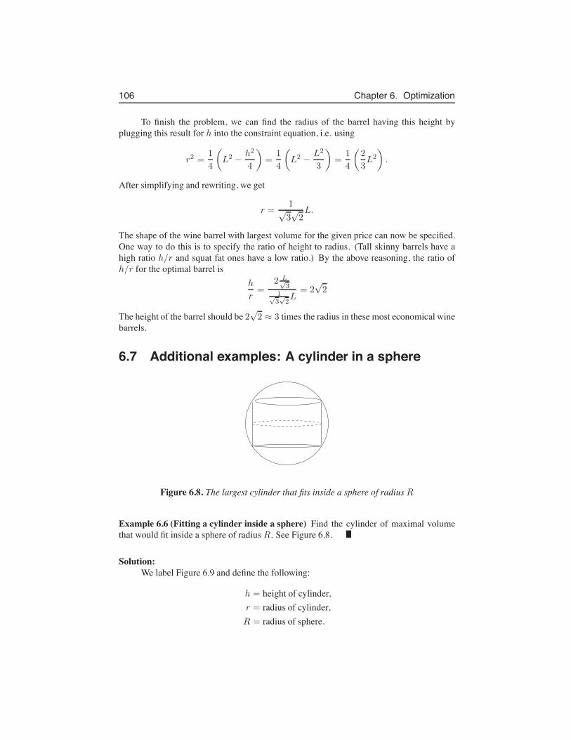
106 Chapter 6. Optimization
To finish the problem, we can find the radius of the barrel having this height byplugging this result for h into the constraint equation, i.e. using
r2 =1
4
(
L2 −h2
4
)
=1
4
(
L2 −L2
3
)
=1
4
(
2
3L2
)
.
After simplifying and rewriting, we get
r =1√3√2L.
The shape of the wine barrel with largest volume for the given price can now be specified.One way to do this is to specify the ratio of height to radius. (Tall skinny barrels have ahigh ratio h/r and squat fat ones have a low ratio.) By the above reasoning, the ratio ofh/r for the optimal barrel is
h
r=
2 L√3
1√3√2L
= 2√2
The height of the barrel should be 2√2 ≈ 3 times the radius in these most economical wine
barrels.
6.7 Additional examples: A cylinder in a sphere
Figure 6.8. The largest cylinder that fits inside a sphere of radius R
Example 6.6 (Fitting a cylinder inside a sphere) Find the cylinder of maximal volumethat would fit inside a sphere of radius R. See Figure 6.8.
Solution:We label Figure 6.9 and define the following:
h = height of cylinder,r = radius of cylinder,R = radius of sphere.
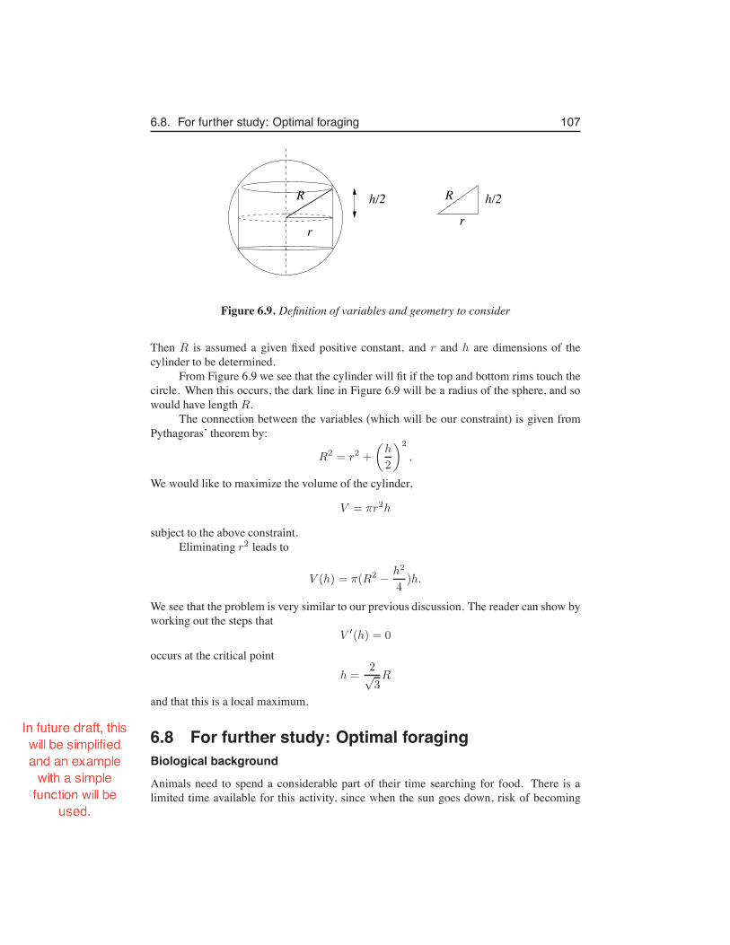
6.8. For further study: Optimal foraging 107
h/2
r
R R h/2r
Figure 6.9. Definition of variables and geometry to consider
Then R is assumed a given fixed positive constant, and r and h are dimensions of thecylinder to be determined.
From Figure 6.9 we see that the cylinder will fit if the top and bottom rims touch thecircle. When this occurs, the dark line in Figure 6.9 will be a radius of the sphere, and sowould have length R.
The connection between the variables (which will be our constraint) is given fromPythagoras’ theorem by:
R2 = r2 +
(
h
2
)2
.
We would like to maximize the volume of the cylinder,
V = πr2h
subject to the above constraint.Eliminating r2 leads to
V (h) = π(R2 −h2
4)h.
We see that the problem is very similar to our previous discussion. The reader can show byworking out the steps that
V ′(h) = 0
occurs at the critical pointh =
2√3R
and that this is a local maximum.
6.8 For further study: Optimal foragingBiological background
Animals need to spend a considerable part of their time searching for food. There is alimited time available for this activity, since when the sun goes down, risk of becoming
Leah Keshet
In future draft, this will be simplified and an example with a simple function will be used.
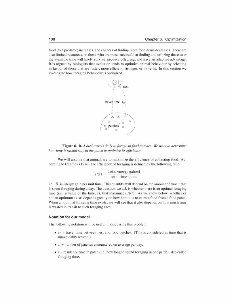
108 Chapter 6. Optimization
food (to a predator) increases, and chances of finding more food items decreases. There arealso limited resources, so those who are most successful at finding and utilizing these overthe available time will likely survive, produce offspring, and have an adaptive advantage.It is argued by biologists that evolution tends to optimize animal behaviour by selectingin favour of those that are faster, more efficient, stronger, or more fit. In this section weinvestigate how foraging behaviour is optimized.
nest
travel time
patchesn
t o
Figure 6.10. A bird travels daily to forage in food patches. We want to determinehow long it should stay in the patch to optimize its efficiency.
We will assume that animals try to maximize the efficiency of collecting food. Ac-cording to Charnov (1976), the efficiency of foraging is defined by the following ratio:
R(t) =Total energy gained
total time spent
i.e., R, is energy gain per unit time. This quantity will depend on the amount of time t thatis spent foraging during a day. The question we ask is whether there is an optimal foragingtime (i.e. a value of the time, t), that maximizes R(t). As we show below, whether ornot an optimum exists depends greatly on how hard it is to extract food from a food patch.When an optimal foraging time exists, we will see that it also depends on how much timeis wasted in transit to such foraging sites.
Notation for our model
The following notation will be useful in discussing this problem:
• t0 = travel time between nest and food patches. (This is considered as time that isunavoidably wasted.)
• n = number of patches encountered on average per day,
• t = residence time in patch (i.e. how long to spend foraging in one patch), also calledforaging time,
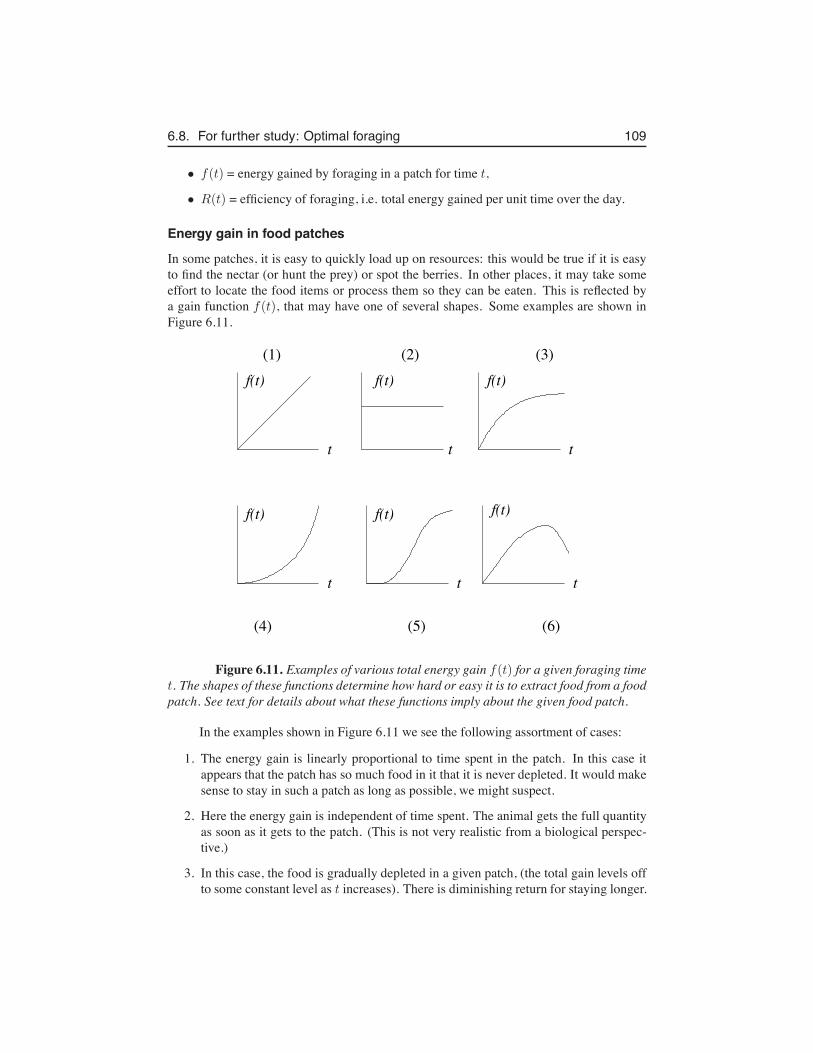
6.8. For further study: Optimal foraging 109
• f(t) = energy gained by foraging in a patch for time t,
• R(t) = efficiency of foraging, i.e. total energy gained per unit time over the day.
Energy gain in food patches
In some patches, it is easy to quickly load up on resources: this would be true if it is easyto find the nectar (or hunt the prey) or spot the berries. In other places, it may take someeffort to locate the food items or process them so they can be eaten. This is reflected bya gain function f(t), that may have one of several shapes. Some examples are shown inFigure 6.11.
t t t
t t t
f(t) f(t) f(t)
f(t) f(t) f(t)
(1) (2) (3)
(4) (5) (6)
Figure 6.11. Examples of various total energy gain f(t) for a given foraging timet. The shapes of these functions determine how hard or easy it is to extract food from a foodpatch. See text for details about what these functions imply about the given food patch.
In the examples shown in Figure 6.11 we see the following assortment of cases:
1. The energy gain is linearly proportional to time spent in the patch. In this case itappears that the patch has so much food in it that it is never depleted. It would makesense to stay in such a patch as long as possible, we might suspect.
2. Here the energy gain is independent of time spent. The animal gets the full quantityas soon as it gets to the patch. (This is not very realistic from a biological perspec-tive.)
3. In this case, the food is gradually depleted in a given patch, (the total gain levels offto some constant level as t increases). There is diminishing return for staying longer.
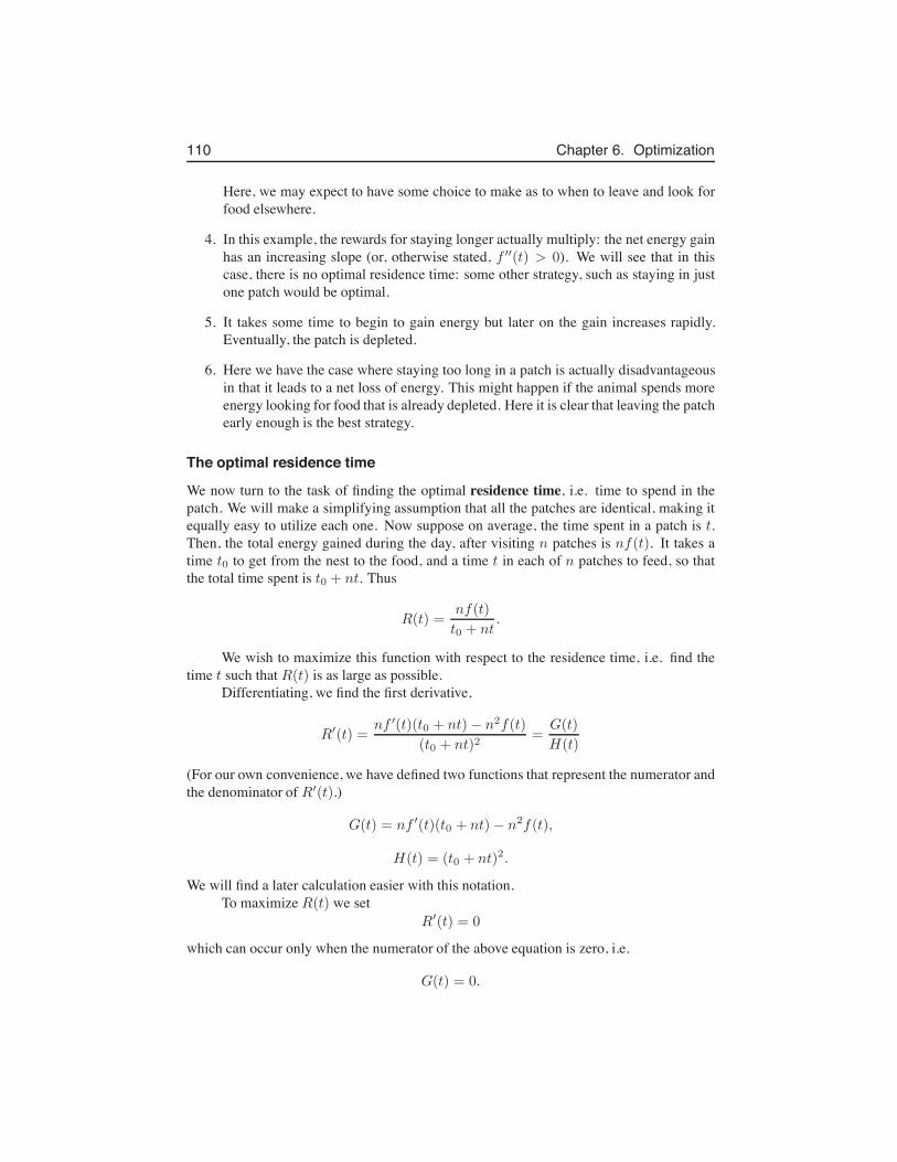
110 Chapter 6. Optimization
Here, we may expect to have some choice to make as to when to leave and look forfood elsewhere.
4. In this example, the rewards for staying longer actually multiply: the net energy gainhas an increasing slope (or, otherwise stated, f ′′(t) > 0). We will see that in thiscase, there is no optimal residence time: some other strategy, such as staying in justone patch would be optimal.
5. It takes some time to begin to gain energy but later on the gain increases rapidly.Eventually, the patch is depleted.
6. Here we have the case where staying too long in a patch is actually disadvantageousin that it leads to a net loss of energy. This might happen if the animal spends moreenergy looking for food that is already depleted. Here it is clear that leaving the patchearly enough is the best strategy.
The optimal residence time
We now turn to the task of finding the optimal residence time, i.e. time to spend in thepatch. We will make a simplifying assumption that all the patches are identical, making itequally easy to utilize each one. Now suppose on average, the time spent in a patch is t.Then, the total energy gained during the day, after visiting n patches is nf(t). It takes atime t0 to get from the nest to the food, and a time t in each of n patches to feed, so thatthe total time spent is t0 + nt. Thus
R(t) =nf(t)
t0 + nt.
We wish to maximize this function with respect to the residence time, i.e. find thetime t such that R(t) is as large as possible.
Differentiating, we find the first derivative,
R′(t) =nf ′(t)(t0 + nt)− n2f(t)
(t0 + nt)2=
G(t)
H(t)
(For our own convenience, we have defined two functions that represent the numerator andthe denominator of R′(t).)
G(t) = nf ′(t)(t0 + nt)− n2f(t),
H(t) = (t0 + nt)2.
We will find a later calculation easier with this notation.To maximize R(t) we set
R′(t) = 0
which can occur only when the numerator of the above equation is zero, i.e.
G(t) = 0.
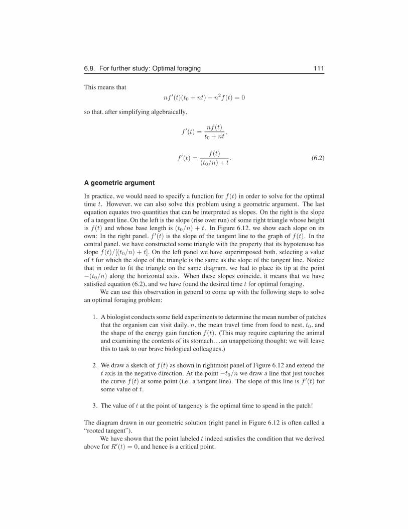
6.8. For further study: Optimal foraging 111
This means thatnf ′(t)(t0 + nt)− n2f(t) = 0
so that, after simplifying algebraically,
f ′(t) =nf(t)
t0 + nt,
f ′(t) =f(t)
(t0/n) + t. (6.2)
A geometric argument
In practice, we would need to specify a function for f(t) in order to solve for the optimaltime t. However, we can also solve this problem using a geometric argument. The lastequation equates two quantities that can be interpreted as slopes. On the right is the slopeof a tangent line, On the left is the slope (rise over run) of some right triangle whose heightis f(t) and whose base length is (t0/n) + t. In Figure 6.12, we show each slope on itsown: In the right panel, f ′(t) is the slope of the tangent line to the graph of f(t). In thecentral panel, we have constructed some triangle with the property that its hypotenuse hasslope f(t)/[(t0/n) + t]. On the left panel we have superimposed both, selecting a valueof t for which the slope of the triangle is the same as the slope of the tangent line. Noticethat in order to fit the triangle on the same diagram, we had to place its tip at the point−(t0/n) along the horizontal axis. When these slopes coincide, it means that we havesatisfied equation (6.2), and we have found the desired time t for optimal foraging.
We can use this observation in general to come up with the following steps to solvean optimal foraging problem:
1. A biologist conducts some field experiments to determine the mean number of patchesthat the organism can visit daily, n, the mean travel time from food to nest, t0, andthe shape of the energy gain function f(t). (This may require capturing the animaland examining the contents of its stomach. . . an unappetizing thought; we will leavethis to task to our brave biological colleagues.)
2. We draw a sketch of f(t) as shown in rightmost panel of Figure 6.12 and extend thet axis in the negative direction. At the point −t0/n we draw a line that just touchesthe curve f(t) at some point (i.e. a tangent line). The slope of this line is f ′(t) forsome value of t.
3. The value of t at the point of tangency is the optimal time to spend in the patch!
The diagram drawn in our geometric solution (right panel in Figure 6.12 is often called a“rooted tangent”).
We have shown that the point labeled t indeed satisfies the condition that we derivedabove for R′(t) = 0, and hence is a critical point.
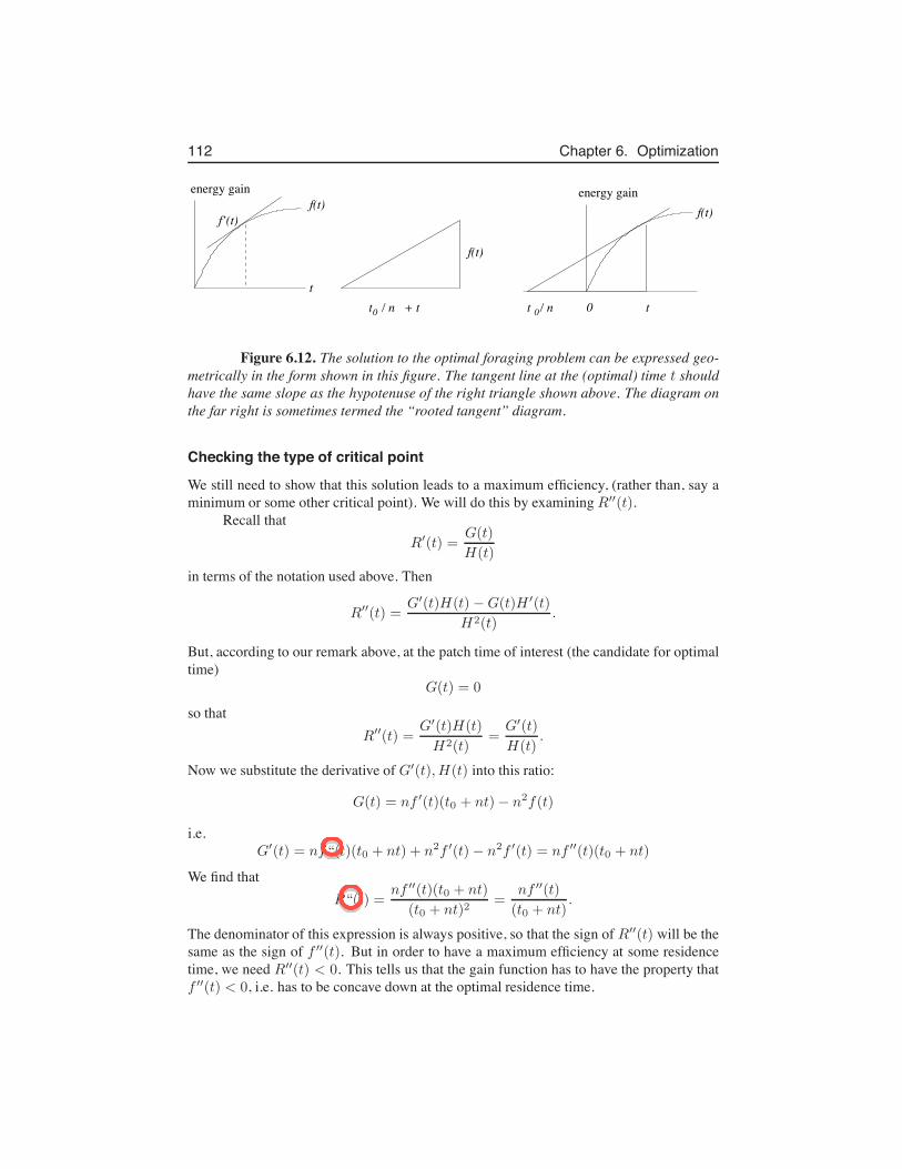
112 Chapter 6. Optimization
00
f(t)
tt / n + t
f(t)f(t)f’(t)
t
energy gain energy gain
0t / n
Figure 6.12. The solution to the optimal foraging problem can be expressed geo-metrically in the form shown in this figure. The tangent line at the (optimal) time t shouldhave the same slope as the hypotenuse of the right triangle shown above. The diagram onthe far right is sometimes termed the “rooted tangent” diagram.
Checking the type of critical point
We still need to show that this solution leads to a maximum efficiency, (rather than, say aminimum or some other critical point). We will do this by examining R′′(t).
Recall thatR′(t) =
G(t)
H(t)
in terms of the notation used above. Then
R′′(t) =G′(t)H(t)−G(t)H ′(t)
H2(t).
But, according to our remark above, at the patch time of interest (the candidate for optimaltime)
G(t) = 0
so thatR′′(t) =
G′(t)H(t)
H2(t)=
G′(t)
H(t).
Now we substitute the derivative of G′(t), H(t) into this ratio:
G(t) = nf ′(t)(t0 + nt)− n2f(t)
i.e.G′(t) = nf“(t)(t0 + nt) + n2f ′(t)− n2f ′(t) = nf ′′(t)(t0 + nt)
We find thatR“(t) =
nf ′′(t)(t0 + nt)
(t0 + nt)2=
nf ′′(t)
(t0 + nt).
The denominator of this expression is always positive, so that the sign of R′′(t) will be thesame as the sign of f ′′(t). But in order to have a maximum efficiency at some residencetime, we need R′′(t) < 0. This tells us that the gain function has to have the property thatf ′′(t) < 0, i.e. has to be concave down at the optimal residence time.
Leah Keshet
Leah Keshet
6.8. For further study: Optimal foraging 113
Going back to some of the shapes of the function f(t) that we discussed in ourexamples, we see that only some of these will lead to an optimal solution. In cases (1),(2), (4) the function f(t) has no points of downwards concavity on its graph. This meansthat in such cases there will be no local maximum. The optimal efficiency would then beattained by spending as much time as possible in just one patch, or as little time as possiblein any patch, i.e. it would be attained at the endpoints.
6.8.1 References:1. Stephens DW, Krebs J R (1986) Foraging Theory, Princeton University Press, Prince-
ton, NJ.
2. Charnov EL (1976) Optimal Foraging: the marginal value theorem; Theor. Pop.Biol. 9 : 129-136.
114 Chapter 6. Optimization
Exercises6.1. The sum of two positive number is 20. Find the numbers
(a) if their product is a maximum.(b) if the sum of their squares is a minimum.(c) if the product of the square of one and the cube of the other is a maximum.
6.2. A tram ride at Disney World departs from its starting place at t = 0 and travelsto the end of its route and back. Its distance from the terminal at time t can beapproximately described by the expression
S(t) = 4t3(10− t)
(where t is in minutes, 0 < t < 10, and S is distance in meters.)(a) Find the velocity as a function of time.(b) When is the tram moving at the fastest rate?(c) At what time does it get to the furthest point away from its starting position?(d) Sketch the acceleration, the velocity, and the position of the tram on the same
set of axes.6.3. At 9A.M., car B is 25 km west of another car A. Car A then travels to the south at
30 km/h and car B travels east at 40 km/h. When will they be the closest to eachother and what is this distance?
6.4. A cannonball is shot vertically upwards from the ground with initial velocity v0 =15m/sec. It is determined that the height of the ball, y (in meters), as a function ofthe time, t (in sec) is given by
y = v0t− 4.9t2
Determine the following:(a) The time at which the cannonball reaches its highest point,(b) The velocity and acceleration of the cannonball at t = 0.5 s, and t = 1.5 s.(c) The time at which the cannonball hits the ground.
6.5. (From Final Exam, Math 100, Dec 1997) A closed 3-dimensional box is to be con-structed in such a way that its volume is 4500 cm3. It is also specified that the lengthof the base is 3 times the width of the base. Find the dimensions of the box whichsatisfy these conditions and have the minimum possible surface area. Justify youranswer.
6.6. A box with a square base is to be made so that its diagonal has length 1. SeeFigure 6.13.
(a) What height y would make the volume maximal?(b) What is the maximal volume?
[Hint: A box having side lengths &, w, h has diagonal length D where D2 =&2 + w2 + h2 and volume V = &wh.]
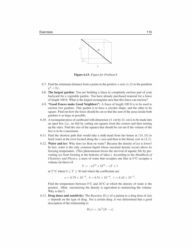
Exercises 115
x
x
Dy
Figure 6.13. Figure for Problem 6
6.7. Find the minimum distance from a point on the positive x-axis (a, 0) to the parabolay2 = 8x.
6.8. The largest garden: You are building a fence to completely enclose part of yourbackyard for a vegetable garden. You have already purchased material for a fenceof length 100 ft. What is the largest rectangular area that this fence can enclose?
6.9. “Good Fences make Good Neighbors”: A fence of length 100 ft is to be used toenclose two gardens. One garden is to have a circular shape, and the other to besquare. Find out how the fence should be cut so that the sum of the areas inside bothgardens is as large as possible.
6.10. A rectangular piece of cardboard with dimension 12 cm by 24 cm is to be made intoan open box (i.e., no lid) by cutting out squares from the corners and then turningup the sides. Find the size of the squares that should be cut out if the volume of thebox is to be a maximum.
6.11. Find the shortest path that would take a milk-maid from her house at (10, 10) tofetch water at the river located along the x axis and then to the thirsty cow at (3, 5).
6.12. Water and ice: Why does ice float on water? Because the density of ice is lower!In fact, water is the only common liquid whose maximal density occurs above itsfreezing temperature. (This phenomenon favors the survival of aquatic life by pre-venting ice from forming at the bottoms of lakes.) According to the Handbook ofChemistry and Physics, a mass of water that occupies one liter at 0◦C occupies avolume (in liters) of
V = −aT 3 + bT 2 − cT + 1
at T ◦C where 0 ≤ T ≤ 30 and where the coefficients are
a = 6.79× 10⁻⁸, b = 8.51× 10⁻⁶, c = 6.42× 10⁻⁵.
Find the temperature between 0◦C and 30◦C at which the density of water is thegreatest. (Hint: maximizing the density is equivalent to minimizing the volume.Why is this?)
6.13. Drug doses and sensitivity: The Reaction R(x) of a patient to a drug dose of sizex depends on the type of drug. For a certain drug, it was determined that a gooddescription of the relationship is:
R(x) = Ax2(B − x)
116 Chapter 6. Optimization
where A and B are positive constants. The Sensitivity of the patient’s body to thedrug is defined to be R′(x).
(a) For what value of x is the reaction a maximum, and what is that maximumreaction value?
(b) For what value of x is the sensitivity a maximum? What is the maximumsensitivity?
6.14. Thermoregulation in a swarm of bees:: In the winter, honeybees sometimes es-cape the hive and form a tight swarm in a tree, where, by shivering, they can produceheat and keep the swarm temperature elevated. Heat energy is lost through the sur-face of the swarm at a rate proportional to the surface area (k1S where k1 > 0 isa constant). Heat energy is produced inside the swarm at a rate proportional to themass of the swarm (which you may take to be a constant times the volume). Wewill assume that the heat production is k2V where k2 > 0 is constant. Swarms thatare not large enough may lose more heat than they can produce, and then they willdie. The heat depletion rate is the loss rate minus the production rate. Assume thatthe swarm is spherical. Find the size of the swarm for which the rate of depletion ofheat energy is greatest.
6.15. A right circular cone is circumscribed about a sphere of radius 5. Find the dimensionof this cone if its volume is to be a minimum. (Remark: this is a rather challenginggeometric problem.)
6.16. Optimal Reproductive Strategy: Animals that can produce many healthy babiesthat survive to the next generation are at an evolutionary advantage over other, com-peting, species. However, too many young produce a heavy burden on the parents(who must feed and care for them). If this causes the parents to die, the advantage islost. Also, competition of the young with one another for food and parental attentionjeopardizes the survival of these babies. Suppose that the evolutionary AdvantageA to the parents of having litter size x is
A(x) = ax− bx2.
Suppose that the Cost C to the parents of having litter size x is
C(x) = mx+ e.
The Net Reproductive Gain G is defined as
G = A− C.
(a) Explain the expressions for A,C and G.(b) At what litter size is the advantage, A, greatest?(c) At what litter size is there least cost to the parents?(d) At what litter size is the Net Reproductive Gain greatest?.
6.17. Behavioural Ecology:: Social animals that live in groups can spend less time scan-ning for predators than solitary individuals. However, they do waste time fighting
Exercises 117
with the other group members over the available food. There is some group sizeat which the net benefit is greatest because the animals spend least time on theseunproductive activities, and thus can spend time on feeding, mating, etc.Assume that for a group of size x, the fraction of time spent scanning for predatorsis
S(x) = A1
(x+ 1)
and the fraction of time spent fighting with other animals over food is
F (x) = B(x + 1)2
where A,B are constants. Find the size of the group for which the time wasted onscanning and fighting is smallest.
6.18. Logistic growth: Consider a fish population whose density (individuals per unitarea) is N . The rate of growth R of this population is found to satisfy
R(N) = rN(1−N/K)
where r and K are positive constants. This type of growth rate is called logistic (ordensity dependent) growth.
(a) Sketch R and a function of N .(b) For what density of fish is the growth rate maximal?
6.19. Logistic growth with harvesting: Consider a fish population of density N growinglogistically, i.e. with rate of growth R(N) = rN(1 − N/K) where r and K arepositive constants. The rate of harvesting (i.e. removal) of the population is
h(N) = qEN
where E, the effort of the fishermen, and q, the catchability of this type of fish, arepositive constants.At what density of fish does the growth rate exactly balance the harvesting rate ?(This density is called the maximal sustainable yield: MSY.)
6.20. Conservation of a harvested population: Conservationists insist that the densityof fish should never be allowed to go below a level at which growth rate of thefish exactly balances with the harvesting rate. (At this level, the harvesting is at itsmaximal sustainable yield. If more fish are taken, the population will keep droppingand the fish will eventually go extinct.) What level of fishing effort should be used tolead to the greatest harvest at this maximal sustainable yield? [Remark: you shouldfirst do the previous problem.]

118 Chapter 6. Optimization
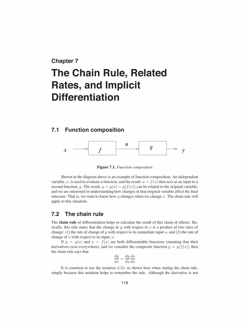
Chapter 7
The Chain Rule, RelatedRates, and ImplicitDifferentiation
7.1 Function composition
xu
yf g
Figure 7.1. Function composition
Shown in the diagram above is an example of function composition: An independentvariable, x, is used to evaluate a function, and the result, u = f(x) then acts as an input to asecond function, g. The result, y = g(u) = g(f(x)) can be related to the original variable,and we are interested in understanding how changes in that original variable affect the finaloutcome: That is, we want to know how y changes when we change x. The chain rule willapply to this situation.
7.2 The chain ruleThe chain rule of differentiation helps to calculate the result of this chain of effects. Ba-sically, this rule states that the change in y with respect to x is a product of two rates ofchange: (1) the rate of change of y with respect to its immediate input u, and (2) the rate ofchange of u with respect to its input, x.
If y = g(u) and u = f(x) are both differentiable functions (meaning that theirderivatives exist everywhere), and we consider the composite function y = g(f(x)) thenthe chain rule says that
dy
dx=
dy
du
du
dx
It is common to use the notation d/dx as shown here when stating the chain rule,simply because this notation helps to remember the rule. Although the derivative is not
119
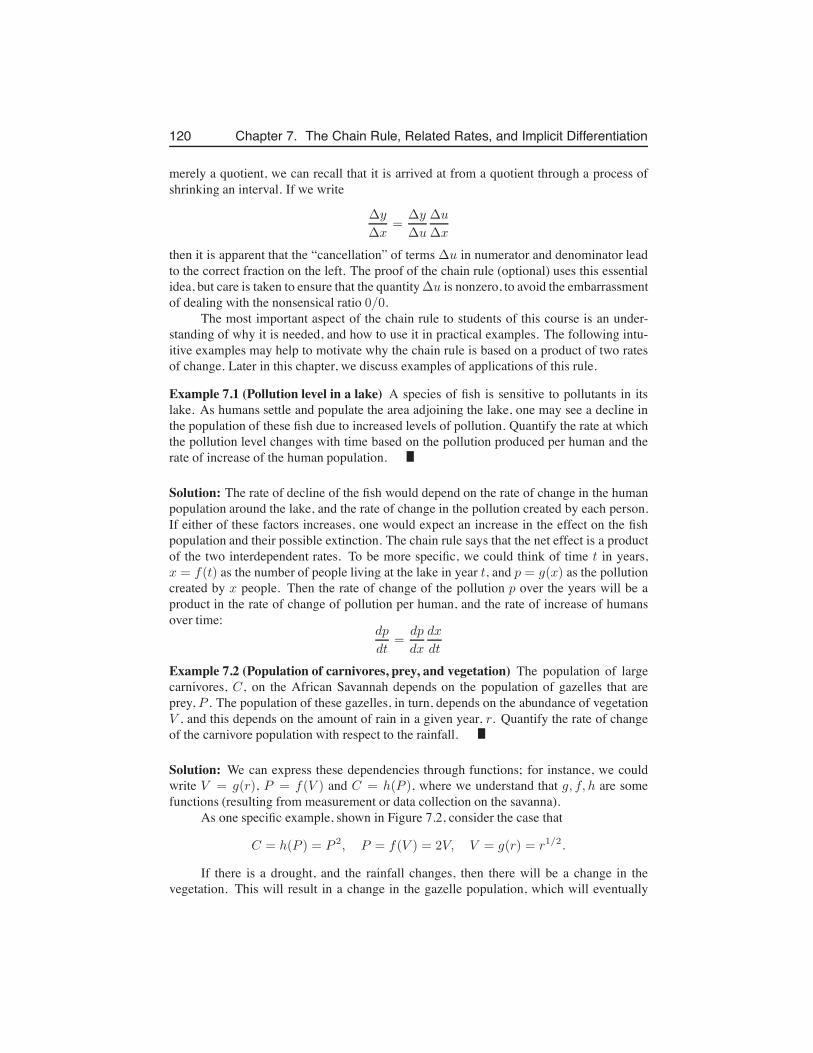
120 Chapter 7. The Chain Rule, Related Rates, and Implicit Differentiation
merely a quotient, we can recall that it is arrived at from a quotient through a process ofshrinking an interval. If we write
∆y
∆x=
∆y
∆u
∆u
∆x
then it is apparent that the “cancellation” of terms ∆u in numerator and denominator leadto the correct fraction on the left. The proof of the chain rule (optional) uses this essentialidea, but care is taken to ensure that the quantity∆u is nonzero, to avoid the embarrassmentof dealing with the nonsensical ratio 0/0.
The most important aspect of the chain rule to students of this course is an under-standing of why it is needed, and how to use it in practical examples. The following intu-itive examples may help to motivate why the chain rule is based on a product of two ratesof change. Later in this chapter, we discuss examples of applications of this rule.
Example 7.1 (Pollution level in a lake) A species of fish is sensitive to pollutants in itslake. As humans settle and populate the area adjoining the lake, one may see a decline inthe population of these fish due to increased levels of pollution. Quantify the rate at whichthe pollution level changes with time based on the pollution produced per human and therate of increase of the human population.
Solution: The rate of decline of the fish would depend on the rate of change in the humanpopulation around the lake, and the rate of change in the pollution created by each person.If either of these factors increases, one would expect an increase in the effect on the fishpopulation and their possible extinction. The chain rule says that the net effect is a productof the two interdependent rates. To be more specific, we could think of time t in years,x = f(t) as the number of people living at the lake in year t, and p = g(x) as the pollutioncreated by x people. Then the rate of change of the pollution p over the years will be aproduct in the rate of change of pollution per human, and the rate of increase of humansover time:
dp
dt=
dp
dx
dx
dt
Example 7.2 (Population of carnivores, prey, and vegetation) The population of largecarnivores, C, on the African Savannah depends on the population of gazelles that areprey, P . The population of these gazelles, in turn, depends on the abundance of vegetationV , and this depends on the amount of rain in a given year, r. Quantify the rate of changeof the carnivore population with respect to the rainfall.
Solution: We can express these dependencies through functions; for instance, we couldwrite V = g(r), P = f(V ) and C = h(P ), where we understand that g, f, h are somefunctions (resulting from measurement or data collection on the savanna).
As one specific example, shown in Figure 7.2, consider the case that
C = h(P ) = P 2, P = f(V ) = 2V, V = g(r) = r1/2.
If there is a drought, and the rainfall changes, then there will be a change in thevegetation. This will result in a change in the gazelle population, which will eventually
7.2. The chain rule 121
r
V
V
P
P
C
Figure 7.2. An example in which the population of carnivores, C = h(P ) =P 2 depends on prey P , while the prey depend on vegetation P = f(V ) = 2V, and thevegetation depends on rainfall V = g(r) = r1/2.
affect the population of carnivores on the savanna. We would like to compute the rate ofchange in the carnivores population with respect to the rainfall, dC/dr.
According to the chain rule,
dC
dr=
dC
dP
dP
dV
dV
dr.
The derivatives we need are
dV
dr=
1
2r−1/2,
dP
dV= 2,
dC
dP= 2P.
so thatdC
dr=
dC
dP
dP
dV
dV
dr=
1
2r−1/2(2)(2P ) =
2P
r1/2.
We can simplify this result by using the fact that V = r1/2 and P = 2V . Plugging thesein, we obtain
dC
dr=
2P
V=
2(2V )
V= 4.
This example is simple enough that we can also express the number of carnivoresexplicitly in terms of rainfall, by using the fact that C = h(P ) = h(f(V )) = h(f(g(r))).We can eliminate all the intermediate variables and express P in terms of r directly:
C = P 2 = (2V )2 = 4V 2 = 4(r1/2)2 = 4r.
(This may be much more cumbersome in more complicated examples.) We can computethe desired derivative in the simple old way, i.e.
dC
dr= 4.
We can see that our two answers agree.
Example 7.3 (Budget for coffee) The budget spent on coffee depends on the number ofcups consumed per day and on the price per cup. The total budget might change if the pricegoes up or if the consumption goes up (e.g. during late nights preparing for midterm ex-ams). Quantify the rate at which your budget for coffee would change if both consumptionand price change.
122 Chapter 7. The Chain Rule, Related Rates, and Implicit Differentiation
Solution: The total rate of change of the coffee budget is a product of the change in theprice and the change in the consumption. (In this example, we might think of time t in daysas the independent variable, x = f(t) as the number of cups of coffee consumed on day t,and y = g(x) as the price for x cups of coffee.)
dy
dt=
dy
dx
dx
dt
7.3 Applications of the chain rule to “related rates”
Volume of sphere V = 43πr
3
Surface area of sphere S = 4πr2
Area of circle A = πr2
Perimeter of circle P = 2πrVolume of cylinder V = πr2h
Volume of cone V = 13πr
2hArea of rectangle A = xy
Perimeter of rectangle P = 2x+ 2yVolume of box V = xyz
Sides of Pythagorean triangle c2 = a2 + b2
Table 7.1. Common relationships on which problems about related rates are often based.
In most of the applications given below, we are interested in processes that take placeover time. We ask how the relationships between certain geometric (or physical) variablesaffects that rates at which they change over time. Many of these examples are given as wordproblems, and we are called on to assemble the required geometric or other relationshipsin solving the problem.
A few relationships that we will find useful are concentrated in Table 7.1 shownbelow
Example 7.4 (Tumor growth:) A tumor grows so that its radius expands at a constantrate, k. Determine the rate of growth of the volume of the tumor when the radius is onecentimeter. Assume that the shape of the tumor is well approximated by a sphere.
Solution: The volume of a sphere of radius r is V = (4/3)πr3. Here both r and V arechanging with time so that
V (t) =4
3π[r(t)]3.
Thusd
dtV (t) =
4
3πd
dt[r(t)]3.
dV
dt=
4
3π3[r(t)]2
dr
dt= 4πr2
dr
dt.
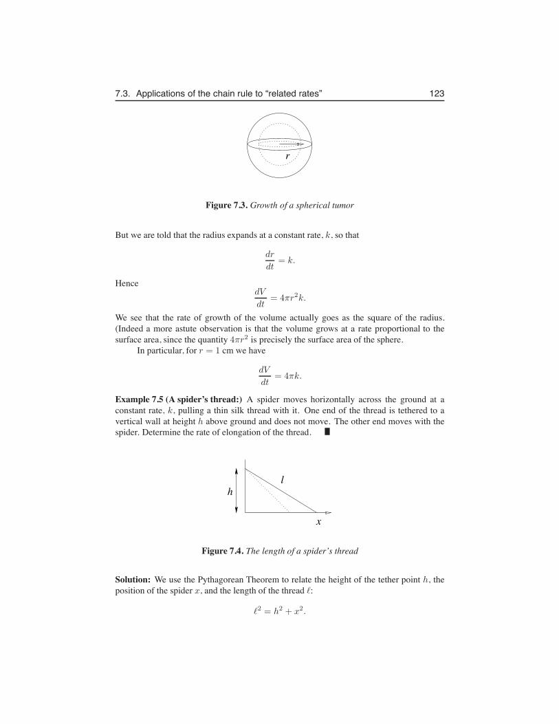
7.3. Applications of the chain rule to “related rates” 123
r
Figure 7.3. Growth of a spherical tumor
But we are told that the radius expands at a constant rate, k, so that
dr
dt= k.
HencedV
dt= 4πr2k.
We see that the rate of growth of the volume actually goes as the square of the radius.(Indeed a more astute observation is that the volume grows at a rate proportional to thesurface area, since the quantity 4πr2 is precisely the surface area of the sphere.
In particular, for r = 1 cm we have
dV
dt= 4πk.
Example 7.5 (A spider’s thread:) A spider moves horizontally across the ground at aconstant rate, k, pulling a thin silk thread with it. One end of the thread is tethered to avertical wall at height h above ground and does not move. The other end moves with thespider. Determine the rate of elongation of the thread.
h
x
l
Figure 7.4. The length of a spider’s thread
Solution: We use the Pythagorean Theorem to relate the height of the tether point h, theposition of the spider x, and the length of the thread &:
&2 = h2 + x2.
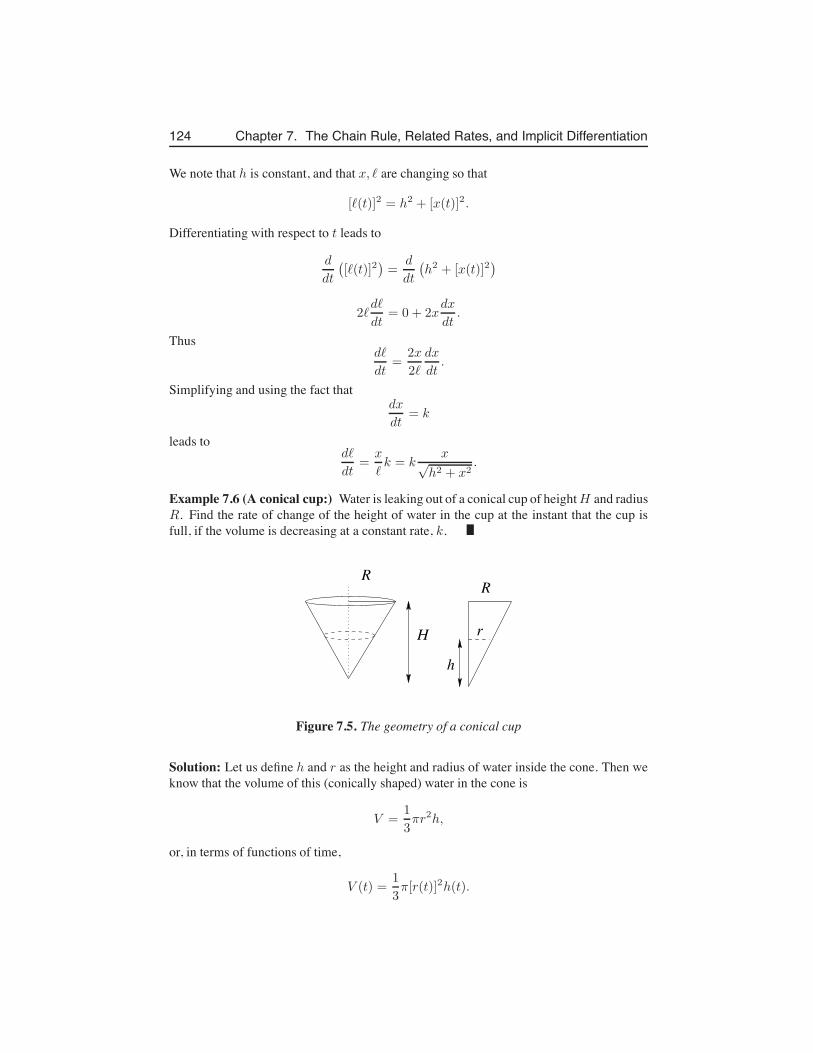
124 Chapter 7. The Chain Rule, Related Rates, and Implicit Differentiation
We note that h is constant, and that x, & are changing so that
[&(t)]2 = h2 + [x(t)]2.
Differentiating with respect to t leads to
d
dt
(
[&(t)]2)
=d
dt
(
h2 + [x(t)]2)
2&d&
dt= 0 + 2x
dx
dt.
Thusd&
dt=
2x
2&
dx
dt.
Simplifying and using the fact thatdx
dt= k
leads tod&
dt=
x
&k = k
x√h2 + x2
.
Example 7.6 (A conical cup:) Water is leaking out of a conical cup of heightH and radiusR. Find the rate of change of the height of water in the cup at the instant that the cup isfull, if the volume is decreasing at a constant rate, k.
H
RR
r
h
Figure 7.5. The geometry of a conical cup
Solution: Let us define h and r as the height and radius of water inside the cone. Then weknow that the volume of this (conically shaped) water in the cone is
V =1
3πr2h,
or, in terms of functions of time,
V (t) =1
3π[r(t)]2h(t).
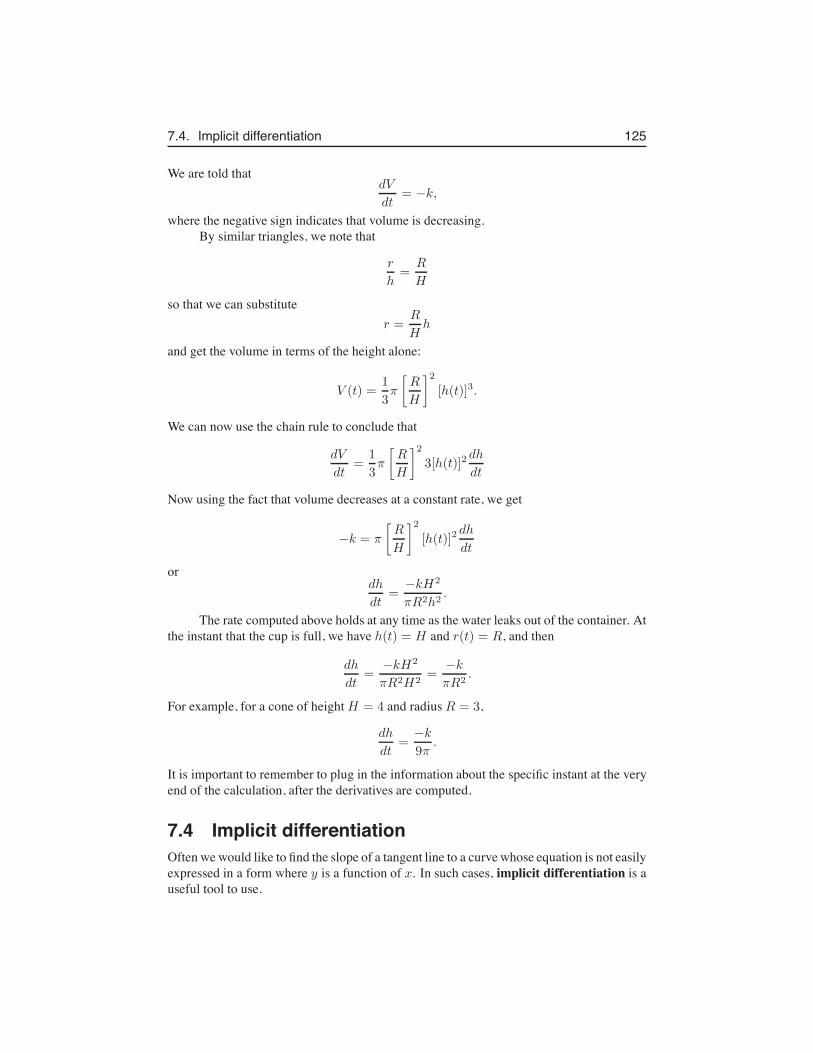
7.4. Implicit differentiation 125
We are told thatdV
dt= −k,
where the negative sign indicates that volume is decreasing.By similar triangles, we note that
r
h=
R
H
so that we can substituter =
R
Hh
and get the volume in terms of the height alone:
V (t) =1
3π
[
R
H
]2
[h(t)]3.
We can now use the chain rule to conclude that
dV
dt=
1
3π
[
R
H
]2
3[h(t)]2dh
dt
Now using the fact that volume decreases at a constant rate, we get
−k = π
[
R
H
]2
[h(t)]2dh
dt
ordh
dt=
−kH2
πR2h2.
The rate computed above holds at any time as the water leaks out of the container. Atthe instant that the cup is full, we have h(t) = H and r(t) = R, and then
dh
dt=
−kH2
πR2H2=
−k
πR2.
For example, for a cone of height H = 4 and radius R = 3,
dh
dt=
−k
9π.
It is important to remember to plug in the information about the specific instant at the veryend of the calculation, after the derivatives are computed.
7.4 Implicit differentiationOften we would like to find the slope of a tangent line to a curve whose equation is not easilyexpressed in a form where y is a function of x. In such cases, implicit differentiation is auseful tool to use.
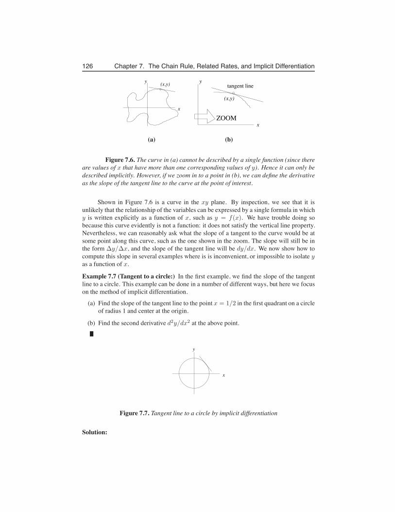
126 Chapter 7. The Chain Rule, Related Rates, and Implicit Differentiation
(x,y)
x
y
x
y
(x,y)
tangent line
ZOOM
(a) (b)
Figure 7.6. The curve in (a) cannot be described by a single function (since thereare values of x that have more than one corresponding values of y). Hence it can only bedescribed implicitly. However, if we zoom in to a point in (b), we can define the derivativeas the slope of the tangent line to the curve at the point of interest.
Shown in Figure 7.6 is a curve in the xy plane. By inspection, we see that it isunlikely that the relationship of the variables can be expressed by a single formula in whichy is written explicitly as a function of x, such as y = f(x). We have trouble doing sobecause this curve evidently is not a function: it does not satisfy the vertical line property.Nevertheless, we can reasonably ask what the slope of a tangent to the curve would be atsome point along this curve, such as the one shown in the zoom. The slope will still be inthe form ∆y/∆x, and the slope of the tangent line will be dy/dx. We now show how tocompute this slope in several examples where is is inconvenient, or impossible to isolate yas a function of x.
Example 7.7 (Tangent to a circle:) In the first example, we find the slope of the tangentline to a circle. This example can be done in a number of different ways, but here we focuson the method of implicit differentiation.
(a) Find the slope of the tangent line to the point x = 1/2 in the first quadrant on a circleof radius 1 and center at the origin.
(b) Find the second derivative d2y/dx2 at the above point.
x
y
Figure 7.7. Tangent line to a circle by implicit differentiation
Solution:
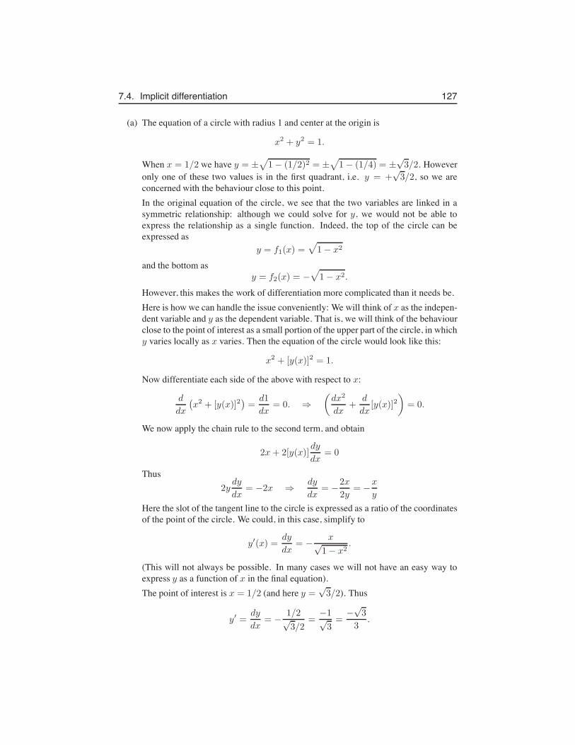
7.4. Implicit differentiation 127
(a) The equation of a circle with radius 1 and center at the origin is
x2 + y2 = 1.
When x = 1/2 we have y = ±√
1− (1/2)2 = ±√
1− (1/4) = ±√3/2. However
only one of these two values is in the first quadrant, i.e. y = +√3/2, so we are
concerned with the behaviour close to this point.In the original equation of the circle, we see that the two variables are linked in asymmetric relationship: although we could solve for y, we would not be able toexpress the relationship as a single function. Indeed, the top of the circle can beexpressed as
y = f1(x) =√
1− x2
and the bottom asy = f2(x) = −
√
1− x2.
However, this makes the work of differentiation more complicated than it needs be.Here is how we can handle the issue conveniently: We will think of x as the indepen-dent variable and y as the dependent variable. That is, we will think of the behaviourclose to the point of interest as a small portion of the upper part of the circle, in whichy varies locally as x varies. Then the equation of the circle would look like this:
x2 + [y(x)]2 = 1.
Now differentiate each side of the above with respect to x:
d
dx
(
x2 + [y(x)]2)
=d1
dx= 0. ⇒
(
dx2
dx+
d
dx[y(x)]2
)
= 0.
We now apply the chain rule to the second term, and obtain
2x+ 2[y(x)]dy
dx= 0
Thus2y
dy
dx= −2x ⇒
dy
dx= −
2x
2y= −
x
y
Here the slot of the tangent line to the circle is expressed as a ratio of the coordinatesof the point of the circle. We could, in this case, simplify to
y′(x) =dy
dx= −
x√1− x2
.
(This will not always be possible. In many cases we will not have an easy way toexpress y as a function of x in the final equation).The point of interest is x = 1/2 (and here y =
√3/2). Thus
y′ =dy
dx= −
1/2√3/2
=−1√3=
−√3
3.
128 Chapter 7. The Chain Rule, Related Rates, and Implicit Differentiation
(b) The second derivative can be computed by differentiating
y′ =dy
dx= −
x
y
We use the quotient rule:d2y
dx2=
d
dx
(
−x
y
)
d2y
dx2= −
1y − xy′
y2= −
y − x−xy
y2= −
y2 + x2
y3= −
1
y3.
Substituting y =√3/2 from part (a) yields
d2y
dx2= −
1
(√3/2)3
= −8
3(3/2).
We have used the equation of the circle, and our previous result for the first deriva-tive in simplifying the above. We can see from this last expression that the secondderivative is negative for y > 0, i.e. for the top semi-circle, indicating that this part ofthe curve is concave down (as expected). Similarly, for y < 0, the second derivativeis positive, and this agrees with the concave up property of that portion of the circle.
As in the case of simple functions, the second derivative can thus help identify con-cavity of curves.
7.5 The power rule for fractional powersImplicit differentiation can help in determining the derivatives of a number of new func-tions. In this case, we use what we know about the integer powers to determine the deriva-tive for a fractional power such as 1/2. A similar idea will recur several times later on inthis course, when we encounter a new type of function and its inverse function.
Example 7.8 (Derivative of√x:) Consider the function
y =√x
Use implicit differentiation to compute the derivative of this function.
Solution: We can re-express this function in the form
y = x1/2.
In this example, we will show that the power rule applies in the same way to fractionalpowers: That is, we show that
y′(x) =1
2x−1/2
7.5. The power rule for fractional powers 129
We rewrite the function y =√x in the form
y2 = x
but we will continue to think of y as the dependent variable, i.e. when we differentiate, wewill remember that
[y(x)]2 = x
Taking derivatives of both sides leads to
d
dx
(
[y(x)]2)
=d
dx(x)
2[y(x)]dy
dx= 1
dy
dx=
1
2y.
We now use the original relationship to eliminate y, i.e. we substitute y =√x. We find
thatdy
dx=
1
2√x=
1
2x−1/2.
This verifies the power law for the above example.A similar procedure can be applied to a power function with fractional power. When
we apply similar steps, we find that
Derivative of fractional-power function: The derivative of
y = f(x) = xm/n
isdy
dx=
m
nx(m
n−1).
This is left as an exercise for the reader.
Example 7.9 Compute the derivative of the function
y = f(x) =√
x2 + a2, where a is some positive real number
Solution: This function can be considered as the composition of g(u) =√u and u(x) =
x2+a2, That is, we can write f(x) = g(h(x)) We rewrite g in the form of a power functionand then use the chain rule to compute the derivative. We obtain
dy
dx=
1
2· (x2 + d2)−1/2 · 2x =
x
(x2 + d2)1/2=
x√x2 + d2
130 Chapter 7. The Chain Rule, Related Rates, and Implicit Differentiation
Example 7.10 Compute the derivative of the function
y = f(x) =x√
x2 + d2, where d is some positive real number
Solution: We use both the quotient rule and the chain rule for this calculation.
dy
dx=
[x]′ ·√x2 + d2 − [
√x2 + d2]′ · x
(√x2 + d2)2
Here the ′ denotes differentiation. Then
dy
dx=
1 ·√x2 + d2 − [ 12 · 2x · (x2 + d2)−1/2] · x
(x2 + d2)
We simplify algebraically by multiplying top and bottom by (x2 + d2)1/2 and cancelingfactors of 2 to obtain
dy
dx=
x2 + d2 − x2
(x2 + d2)1/2(x2 + d2)=
d2
(x2 + d2)3/2
Example 7.11 (The astroid:) The curve
x2/3 + y2/3 = 22/3
has the shape of an astroid. It describes the shape generated by a ball of radius 12 rolling
inside a ball of radius 2. Find the slope of the tangent line to a point on the astroid.
Solution: We use implicit differentiation as follows:d
dx
(
x2/3 + y2/3)
=d
dx22/3
2
3x−1/3 +
d
dy(y2/3)
dy
dx= 0
2
3x−1/3 +
2
3y−1/3 dy
dx= 0
x−1/3 + y−1/3 dy
dx= 0
We can rearrange into the form:
dy
dx= −
x−1/3
y−1/3.
We can see from this form that the derivative fails to exist at both x = 0 (where x−1/3
would be undefined) and at y = 0 (where y−1/3 would be undefined. This stems from thesharp points that the curve has at these places.
In the next example we put the second derivative to work in an implicit differentiationproblem. The goal is as follows:
7.5. The power rule for fractional powers 131
Example 7.12 (Horizontal tangent and concavity on a rotated ellipse:) Find the highestpoint on the (rotated) ellipse
x2 + 3y2 − xy = 1
Solution: The highest point on the ellipse will have a horizontal tangent line, so we shouldlook for the point on this curve at which dy/dx = 0. We proceed as follows:
1. Finding the slope of the tangent line: By implicit differentiation,
d
dx[x2 + 3y2 − xy] =
d
dx1
d(x2)
dx+
d(3y2)
dx−
d(xy)
dx= 0.
We must use the product rule to compute the derivative of the last term on the LHS:
2x+ 6ydy
dx− x
dy
dx−
dx
dxy = 0
2x+ 6ydy
dx− x
dy
dx− 1y = 0
Grouping terms, we have
(6y − x)dy
dx+ (2x− y) = 0
Thusdy
dx=
(y − 2x)
(6y − x).
We can also use the notation
y′(x) =(y − 2x)
(6y − x)
to denote the derivative. Setting dy/dx = 0, we obtain y − 2x = 0 so that y = 2xat the point of interest. However, we still need to find the coordinates of the pointsatisfying this condition.
2. Determining the coordinates of the point we want: To do so, we look for a pointthat satisfies the equation of the curve as well as the condition y = 2x. Plugging intothe original equation of the ellipse, we get:
x2 + 3y2 − xy = 1
x2 + 3(2x)2 − x(2x) = 1.
After simplifying, this equation becomes 11x2 = 1, leading to the two possibilities
x = ±1√11
, y = ±2√11
.
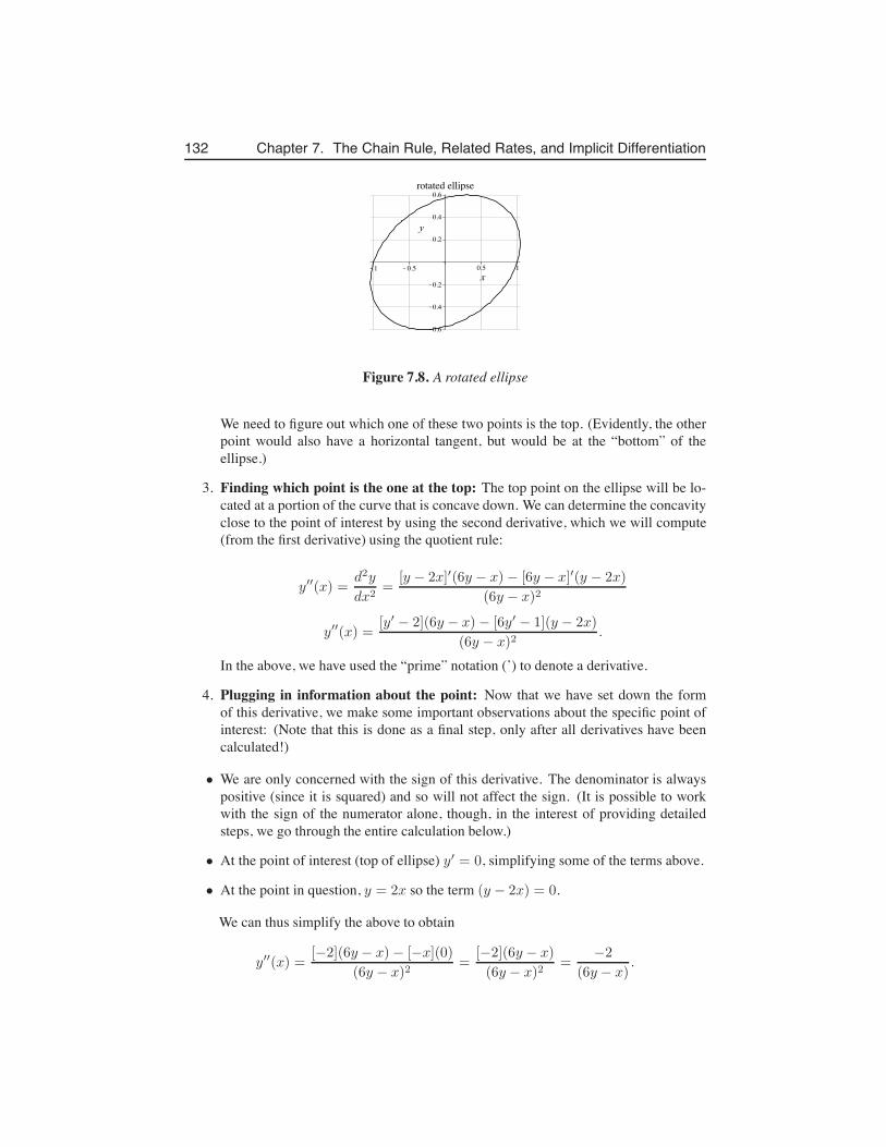
132 Chapter 7. The Chain Rule, Related Rates, and Implicit Differentiation
Figure 7.8. A rotated ellipse
We need to figure out which one of these two points is the top. (Evidently, the otherpoint would also have a horizontal tangent, but would be at the “bottom” of theellipse.)
3. Finding which point is the one at the top: The top point on the ellipse will be lo-cated at a portion of the curve that is concave down. We can determine the concavityclose to the point of interest by using the second derivative, which we will compute(from the first derivative) using the quotient rule:
y′′(x) =d2y
dx2=
[y − 2x]′(6y − x)− [6y − x]′(y − 2x)
(6y − x)2
y′′(x) =[y′ − 2](6y − x)− [6y′ − 1](y − 2x)
(6y − x)2.
In the above, we have used the “prime” notation (’) to denote a derivative.
4. Plugging in information about the point: Now that we have set down the formof this derivative, we make some important observations about the specific point ofinterest: (Note that this is done as a final step, only after all derivatives have beencalculated!)
• We are only concerned with the sign of this derivative. The denominator is alwayspositive (since it is squared) and so will not affect the sign. (It is possible to workwith the sign of the numerator alone, though, in the interest of providing detailedsteps, we go through the entire calculation below.)
• At the point of interest (top of ellipse) y′ = 0, simplifying some of the terms above.
• At the point in question, y = 2x so the term (y − 2x) = 0.
We can thus simplify the above to obtain
y′′(x) =[−2](6y − x)− [−x](0)
(6y − x)2=
[−2](6y − x)
(6y − x)2=
−2
(6y − x).
7.6. Food choice and attention 133
Using again the fact that y = 2x, we get the final form
y′′(x) =−2
(6(2x)− x)=
−2
11x.
We see directly from this result that the second derivative is negative (implying concavedown curve) whenever x is positive. This tells us that at the point with positive x value,x = 1/
√11, we are at the top of the ellipse. A graph of this curve is shown in Figure 7.8.
7.6 Food choice and attentionThe example described in this section is taken from actual biological research. It has severalnoteworthy features: First, we do put the chain rule to use in the problem. Second, weencounter a surprise in some of our elementary calculations. Third, we find that not everyproblem has an elegant or analytically simple solution. Finally, we see that some verygeneral observations can provide insight that we do not get as easily from the specificcases. The problem is taken from the study of animal behaviour.
Paying attention
Behavioural ecologist Reuven Dukas (McMaster U) studies the choices that animals makewhen deciding which food to look for. His work has resulted in both theoretical and ex-perimental conclusions about choices and strategies that animals follow. The example de-scribed below is based on his work with blue jays described in several publications. (Seereferences.)
Many types of food are cryptic, i.e. hidden in the environment, and require timeand attention to find. Some types of food are more easy to detect than other types, andsome foods provide more nourishment than other types. Clearly, the animal that succeedsin gaining the greatest nourishment during a typical day will have a greater chance ofsurviving and out-competing others. Thus, it makes sense that animals should chose todivide their time and attention between food types in such a way as to maximize the totalgain over the given time period available for foraging.
Setting up a model
Suppose that there are two types of food available in the environment. We will define avariable that represents the attention that an animal can devote to finding a given food type.
• Let x = attention devoted to finding food of some type. Assume that 0 < x < 1, withx = 0 representing no attention at all to that type of food and x = 1 full attentiondevoted to finding that item.
• Let P (x) denote the probability of finding the food given that attention x is devotedto the task. Then 0 < P < 1, as is commonly assumed for a probability. P = 0means that the food is never found, and P = 1 means that the food is always found.
• Consider foods that have the property P (0) = 0, P (1) = 1. This means that if noattention is payed (x = 0) then there is no probability of finding the food (P = 0),
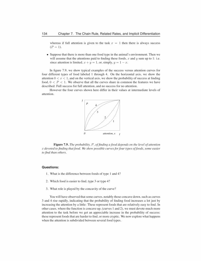
134 Chapter 7. The Chain Rule, Related Rates, and Implicit Differentiation
whereas if full attention is given to the task x = 1 then there is always success(P = 1).
• Suppose that there is more than one food type in the animal’s environment. Then wewill assume that the attentions paid to finding these foods, x and y sum up to 1: i.e.since attention is limited, x+ y = 1, or, simply, y = 1− x.
In figure 7.9, we show typical examples of the success versus attention curves forfour different types of food labeled 1 through 4. On the horizontal axis, we show theattention 0 < x < 1, and on the vertical axis, we show the probability of success at findingfood, 0 < P < 1. We observe that all the curves share in common the features we havedescribed: Full success for full attention, and no success for no attention.
However the four curves shown here differ in their values at intermediate levels ofattention.
0 1
1P
attention, x
12
3
4
Figure 7.9. The probability, P , of finding a food depends on the level of attentionx devoted to finding that food. We show possible curves for four types of foods, some easierto find than others.
Questions:
1. What is the difference between foods of type 1 and 4?
2. Which food is easier to find, type 3 or type 4?
3. What role is played by the concavity of the curve?
You will have observed that some curves, notably those concave down, such as curves3 and 4 rise rapidly, indicating that the probability of finding food increases a lot just byincreasing the attention by a little: These represent foods that are relatively easy to find. Inother cases, where the function is concave up, (curves 1 and 2), we must devote much moreattention to the task before we get an appreciable increase in the probability of success:these represent foods that are harder to find, or more cryptic. We now explore what happenswhen the attention is subdivided between several food types.
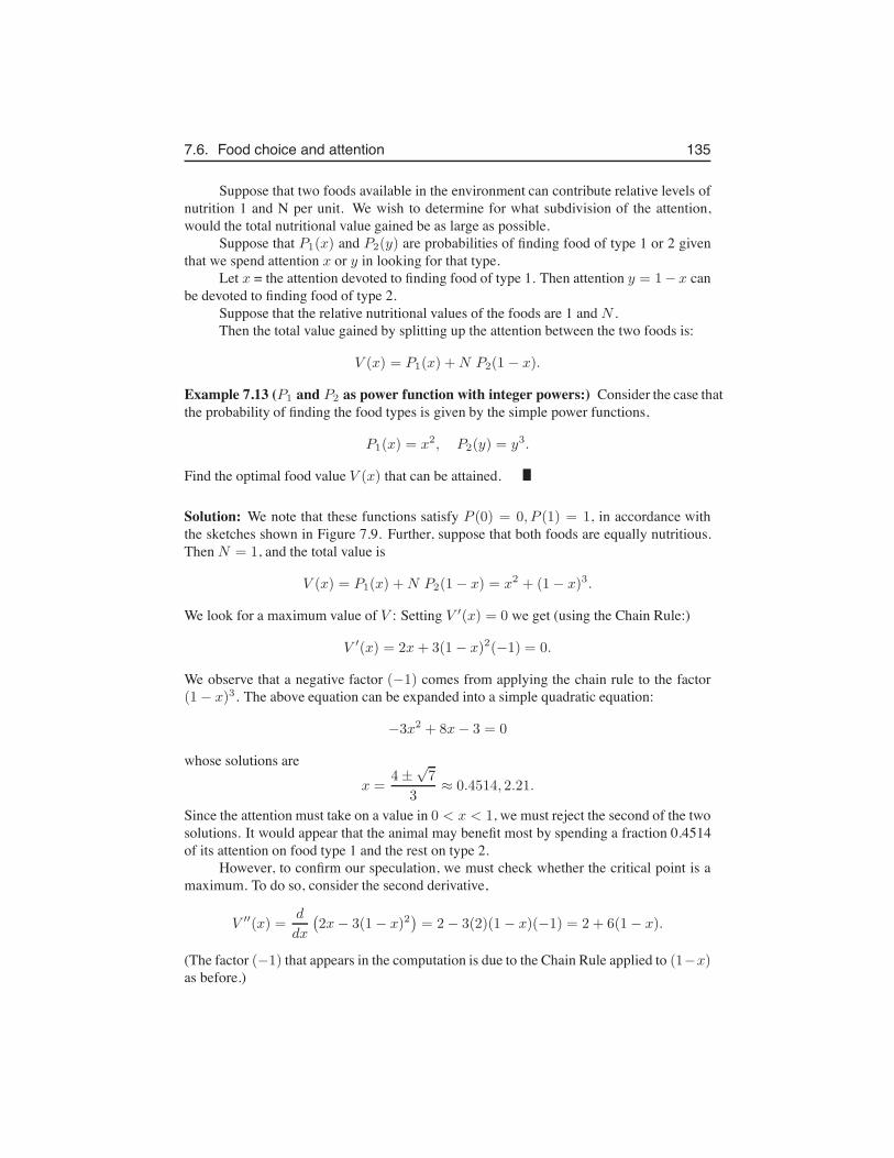
7.6. Food choice and attention 135
Suppose that two foods available in the environment can contribute relative levels ofnutrition 1 and N per unit. We wish to determine for what subdivision of the attention,would the total nutritional value gained be as large as possible.
Suppose that P1(x) and P2(y) are probabilities of finding food of type 1 or 2 giventhat we spend attention x or y in looking for that type.
Let x = the attention devoted to finding food of type 1. Then attention y = 1− x canbe devoted to finding food of type 2.
Suppose that the relative nutritional values of the foods are 1 and N .Then the total value gained by splitting up the attention between the two foods is:
V (x) = P1(x) +N P2(1 − x).
Example 7.13 (P1 and P2 as power function with integer powers:) Consider the case thatthe probability of finding the food types is given by the simple power functions,
P1(x) = x2, P2(y) = y3.
Find the optimal food value V (x) that can be attained.
Solution: We note that these functions satisfy P (0) = 0, P (1) = 1, in accordance withthe sketches shown in Figure 7.9. Further, suppose that both foods are equally nutritious.Then N = 1, and the total value is
V (x) = P1(x) +N P2(1− x) = x2 + (1− x)3.
We look for a maximum value of V : Setting V ′(x) = 0 we get (using the Chain Rule:)
V ′(x) = 2x+ 3(1− x)2(−1) = 0.
We observe that a negative factor (−1) comes from applying the chain rule to the factor(1− x)3. The above equation can be expanded into a simple quadratic equation:
−3x2 + 8x− 3 = 0
whose solutions are
x =4±
√7
3≈ 0.4514, 2.21.
Since the attention must take on a value in 0 < x < 1, we must reject the second of the twosolutions. It would appear that the animal may benefit most by spending a fraction 0.4514of its attention on food type 1 and the rest on type 2.
However, to confirm our speculation, we must check whether the critical point is amaximum. To do so, consider the second derivative,
V ′′(x) =d
dx
(
2x− 3(1− x)2)
= 2− 3(2)(1− x)(−1) = 2 + 6(1− x).
(The factor (−1) that appears in the computation is due to the Chain Rule applied to (1−x)as before.)
136 Chapter 7. The Chain Rule, Related Rates, and Implicit Differentiation
Observing the result, and recalling that x < 1, we note that the second derivativeis positive for all values of x! This is unfortunate, as it signifies a local minimum! Theanimal gains least by splitting up its attention between the foods in this case. Indeed, fromFigure 7.10(a), we see that the most gain occurs at either x = 0 (only food of type 2 sought)or x = 1 (only food of type 1 sought). Again we observe the importance of checking forthe type of critical point before drawing hasty conclusions.
V1(x)
0.0 1.00.0
1.0
V2(x)
0.0 1.01.0
1.6
(a) (b)
Figure 7.10. (a) Figure for Example 7.13 and (b) for Example 7.14
Example 7.14 (Fractional-power functions for P1, P2:) As a second example, considerthe case that the probability of finding the food types is given by the concave down powerfunctions,
P1(x) = x1/2, P2(y) = y1/3
and both foods are equally nutritious (N = 1). Find the optimal food value V (x).
Solution: These functions also satisfy P (0) = 0, P (1) = 1, in accordance with thesketches shown in Figure 7.9. Then
V (x) = P1(x) + P2(1− x) =√x+ (1 − x)(1/3),
V ′(x) =1
2√x−
1
3 (1.0− x)(2/3),
V ′′(x) = −1
4 x(3/2)−
2
9 (1.0− x)(5/3).
Calculations to actually determine the critical point are rather ugly, and best handled nu-merically. We state without details the fact that a critical point occurs at x = 0.61977 (andy = 1 − x = 0.38022.) within the interval of interest. A plotting program is used to dis-play the Value obtained by splitting up the attention in this way in Figure 7.10(b). It is clear
Leah Keshet
7.7. Shortest path from food to nest 137
from this figure that a maximum occurs in the middle of the interval, i.e for attention splitbetween finding both foods. We further see from V ′′(x) that the second derivative is neg-ative for all values of x in the interval, indicating that we have obtained a local maximum,as expected.
Epilogue
While the conclusions drawn above were disappointing in one specific case, it is not alwaystrue that concentrating all one’s attention on one type is optimal. We can examine theproblem in more generality to find when the opposite conclusion might be satisfied. In thegeneral case, the value gained is
V (x) = P1(x) +N P2(1 − x).
A critical point occurs when
V ′(x) =d
dx[P1(x) +N P2(1− x)] = P ′
1(x) +NP ′2(1− x)(−1) = 0.
(By now you realize where the extra term (−1) comes from - yes, from the Chain Rule!)Suppose we have found a value of x in 0 < x < 1 at which this is satisfied. We thenexamine the second derivative:
V ′′(x) =d
dx[V ′(x)] =
d
dx[P ′
1(x)−NP ′2(1− x)]
= P ′′1 (x) −NP ′′
2 (1− x)(−1) = P ′′1 (x) +NP ′′
2 (1− x).
The concavity of the function V is thus related to the concavity of the two functions P1(x)and P2(1− x). If these are concave down (e.g. as in food types 3 or 4 in Figure 7.9), thenV ′′(x) < 0 and a local maximum will occur at any critical point found by our differentia-tion.
Another way of stating this observation is: if both food types are relatively easy tofind, one can gain most benefit by splitting up the attention between the two. Otherwise, ifboth are hard to find, then it is best to look for only one at a time.
7.7 Shortest path from food to nestAnts are good mathematicians! They are able to find the shortest route that connects theirnest to a food source, to be as efficient as possible in bringing the food back home.
But how do they do it? It transpires that each ant secretes a chemical pheromonethat other ants like to follow. This marks up the trail that they use, and recruits nest-mates to food sources. The pheromone (chemical message for marking a route) evaporatesafter a while, so that, for a given number of foraging ants, a longer trail will have a lessconcentrated chemical marking than a shorter trail. This means that whenever a shorterroute is found, the ants will favour it. After some time, this leads to selection of the shortestpossible trail.
Shown in the figure below is a common laboratory test scenario, where ants at a nestare offered two equivalent food sources to utilize. We will use the chain rule and other
Leah Keshet
consider also variant where ants mark trails differently and/or number of ants on given path is considered
Leah Keshet
Leah Keshet
As we have seen in the second example,
Leah Keshet
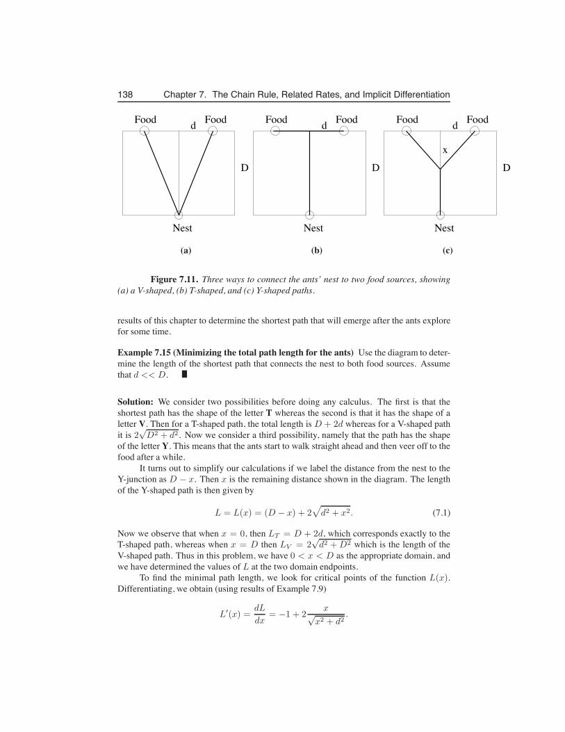
138 Chapter 7. The Chain Rule, Related Rates, and Implicit Differentiation
Food
Nest
D
d Food Food
Nest
D
d Food Food
Nest
Dx
d Food
(a) (b) (c)
Figure 7.11. Three ways to connect the ants’ nest to two food sources, showing(a) a V-shaped, (b) T-shaped, and (c) Y-shaped paths.
results of this chapter to determine the shortest path that will emerge after the ants explorefor some time.
Example 7.15 (Minimizing the total path length for the ants) Use the diagram to deter-mine the length of the shortest path that connects the nest to both food sources. Assumethat d << D.
Solution: We consider two possibilities before doing any calculus. The first is that theshortest path has the shape of the letter T whereas the second is that it has the shape of aletter V. Then for a T-shaped path, the total length is D + 2d whereas for a V-shaped pathit is 2
√D2 + d2. Now we consider a third possibility, namely that the path has the shape
of the letter Y. This means that the ants start to walk straight ahead and then veer off to thefood after a while.
It turns out to simplify our calculations if we label the distance from the nest to theY-junction as D − x. Then x is the remaining distance shown in the diagram. The lengthof the Y-shaped path is then given by
L = L(x) = (D − x) + 2√
d2 + x2. (7.1)
Now we observe that when x = 0, then LT = D + 2d, which corresponds exactly to theT-shaped path, whereas when x = D then LV = 2
√d2 +D2 which is the length of the
V-shaped path. Thus in this problem, we have 0 < x < D as the appropriate domain, andwe have determined the values of L at the two domain endpoints.
To find the minimal path length, we look for critical points of the function L(x).Differentiating, we obtain (using results of Example 7.9)
L′(x) =dL
dx= −1 + 2
x√x2 + d2
.
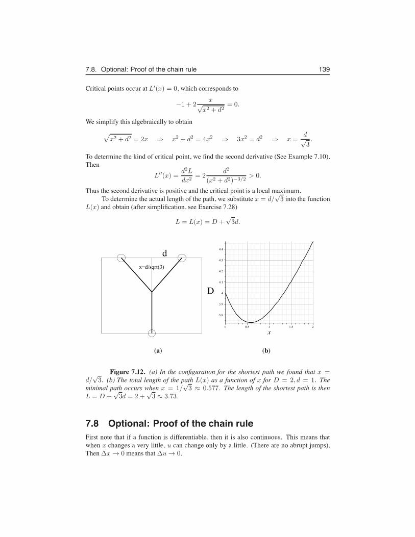
7.8. Optional: Proof of the chain rule 139
Critical points occur at L′(x) = 0, which corresponds to
−1 + 2x√
x2 + d2= 0.
We simplify this algebraically to obtain√
x2 + d2 = 2x ⇒ x2 + d2 = 4x2 ⇒ 3x2 = d2 ⇒ x =d√3.
To determine the kind of critical point, we find the second derivative (See Example 7.10).Then
L′′(x) =d2L
dx2= 2
d2
(x2 + d2)−3/2> 0.
Thus the second derivative is positive and the critical point is a local maximum.To determine the actual length of the path, we substitute x = d/
√3 into the function
L(x) and obtain (after simplification, see Exercise 7.28)
L = L(x) = D +√3d.
x=d/sqrt(3)
D
d
(a) (b)
Figure 7.12. (a) In the configuration for the shortest path we found that x =d/
√3. (b) The total length of the path L(x) as a function of x for D = 2, d = 1. The
minimal path occurs when x = 1/√3 ≈ 0.577. The length of the shortest path is then
L = D +√3d = 2 +
√3 ≈ 3.73.
7.8 Optional: Proof of the chain ruleFirst note that if a function is differentiable, then it is also continuous. This means thatwhen x changes a very little, u can change only by a little. (There are no abrupt jumps).Then ∆x → 0 means that ∆u → 0.
140 Chapter 7. The Chain Rule, Related Rates, and Implicit Differentiation
Now consider the definition of the derivative dy/du:
dy
du= lim
∆u→0
∆y
∆u
This means that for any (finite) ∆u,
∆y
∆u=
dy
du+ ε
where ε → 0 as ∆u → 0. Then
∆y =dy
du∆u + ε∆u
Now divide both sides by some (nonzero) ∆x: Then
∆y
∆x=
dy
du
∆u
∆x+ ε
∆u
∆x
Taking ∆x → 0 we get ∆u → 0, (by continuity) and hence also ε → 0 so that as desired,
dy
dx=
dy
du
du
dx
• Dukas R, Kamil A C(2001) Limited attention: The constraint underlying search im-age. Behavioral Ecology. 12(2): 192-199.
• Dukas R; Kamil A C (2000) The cost of limited attention in blue jays. BehavioralEcology 11(5): 502-506.
• Dukas R, Ellner S, (1993) Information processing and prey detection. Ecology.74(5): 1337-1346.
Exercises 141
Exercises7.1. For each of the following, find the derivative of y with respect to x.
(a) y6 + 3y − 2x− 7x3 = 0
(b) ey + 2xy =√3
(c) y = xcos x
7.2. Consider the growth of a cell, assumed spherical in shape. Suppose that the radiusof the cell increases at a constant rate per unit time. (Call the constant k, and assumethat k > 0.)
(a) At what rate would the volume, V , increase ?(b) At what rate would the surface area, S, increase ?(c) At what rate would the ratio of surface area to volume S/V change? Would
this ratio increase or decrease as the cell grows? [Remark: note that the an-swers you give will be expressed in terms of the radius of the cell.]
7.3. Growth of a circular fungal colony: A fungal colony grows on a flat surface start-ing with a single spore. The shape of the colony edge is circular (with the initial siteof the spore at the center of the circle.) Suppose the radius of the colony increasesat a constant rate per unit time. (Call this constant C.)
(a) At what rate does the area covered by the colony change ?(b) The biomass of the colony is proportional to the area it occupies (factor of
proportionality α). At what rate does the biomass increase?7.4. Limb development: During early development, the limb of a fetus increases in size,
but has a constant proportion. Suppose that the limb is roughly a circular cylinderwith radius r and length l in proportion
l/r = C
where C is a positive constant. It is noted that during the initial phase of growth, theradius increases at an approximately constant rate, i.e. that
dr/dt = a.
At what rate does the mass of the limb change during this time? [Note: assume thatthe density of the limb is 1 gm/cm3 and recall that the volume of a cylinder is
V = Al
where A is the base area (in this case of a circle) and l is length.]7.5. A rectangular trough is 2 meter long, 0.5 meter across the top and 1 meter deep. At
what rate must water be poured into the trough such that the depth of the water isincreasing at 1 m/min when the depth of the water is 0.7 m?
7.6. Gas is being pumped into a spherical balloon at the rate of 3 cm3/s.
Leah Keshet
Leah Keshet
these questions will be modified to avoid using exp and cos, whose derivatives are discussed later.
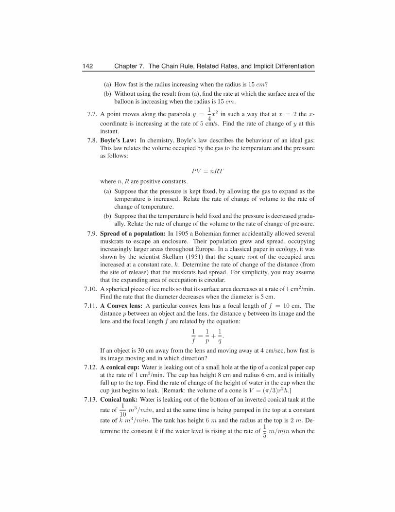
142 Chapter 7. The Chain Rule, Related Rates, and Implicit Differentiation
(a) How fast is the radius increasing when the radius is 15 cm?(b) Without using the result from (a), find the rate at which the surface area of the
balloon is increasing when the radius is 15 cm.
7.7. A point moves along the parabola y =1
4x2 in such a way that at x = 2 the x-
coordinate is increasing at the rate of 5 cm/s. Find the rate of change of y at thisinstant.
7.8. Boyle’s Law: In chemistry, Boyle’s law describes the behaviour of an ideal gas:This law relates the volume occupied by the gas to the temperature and the pressureas follows:
PV = nRT
where n,R are positive constants.(a) Suppose that the pressure is kept fixed, by allowing the gas to expand as the
temperature is increased. Relate the rate of change of volume to the rate ofchange of temperature.
(b) Suppose that the temperature is held fixed and the pressure is decreased gradu-ally. Relate the rate of change of the volume to the rate of change of pressure.
7.9. Spread of a population: In 1905 a Bohemian farmer accidentally allowed severalmuskrats to escape an enclosure. Their population grew and spread, occupyingincreasingly larger areas throughout Europe. In a classical paper in ecology, it wasshown by the scientist Skellam (1951) that the square root of the occupied areaincreased at a constant rate, k. Determine the rate of change of the distance (fromthe site of release) that the muskrats had spread. For simplicity, you may assumethat the expanding area of occupation is circular.
7.10. A spherical piece of ice melts so that its surface area decreases at a rate of 1 cm2/min.Find the rate that the diameter decreases when the diameter is 5 cm.
7.11. A Convex lens: A particular convex lens has a focal length of f = 10 cm. Thedistance p between an object and the lens, the distance q between its image and thelens and the focal length f are related by the equation:
1
f=
1
p+
1
q.
If an object is 30 cm away from the lens and moving away at 4 cm/sec, how fast isits image moving and in which direction?
7.12. A conical cup: Water is leaking out of a small hole at the tip of a conical paper cupat the rate of 1 cm3/min. The cup has height 8 cm and radius 6 cm, and is initiallyfull up to the top. Find the rate of change of the height of water in the cup when thecup just begins to leak. [Remark: the volume of a cone is V = (π/3)r2h.]
7.13. Conical tank: Water is leaking out of the bottom of an inverted conical tank at therate of 1
10m3/min, and at the same time is being pumped in the top at a constant
rate of k m3/min. The tank has height 6 m and the radius at the top is 2 m. De-termine the constant k if the water level is rising at the rate of 1
5m/min when the
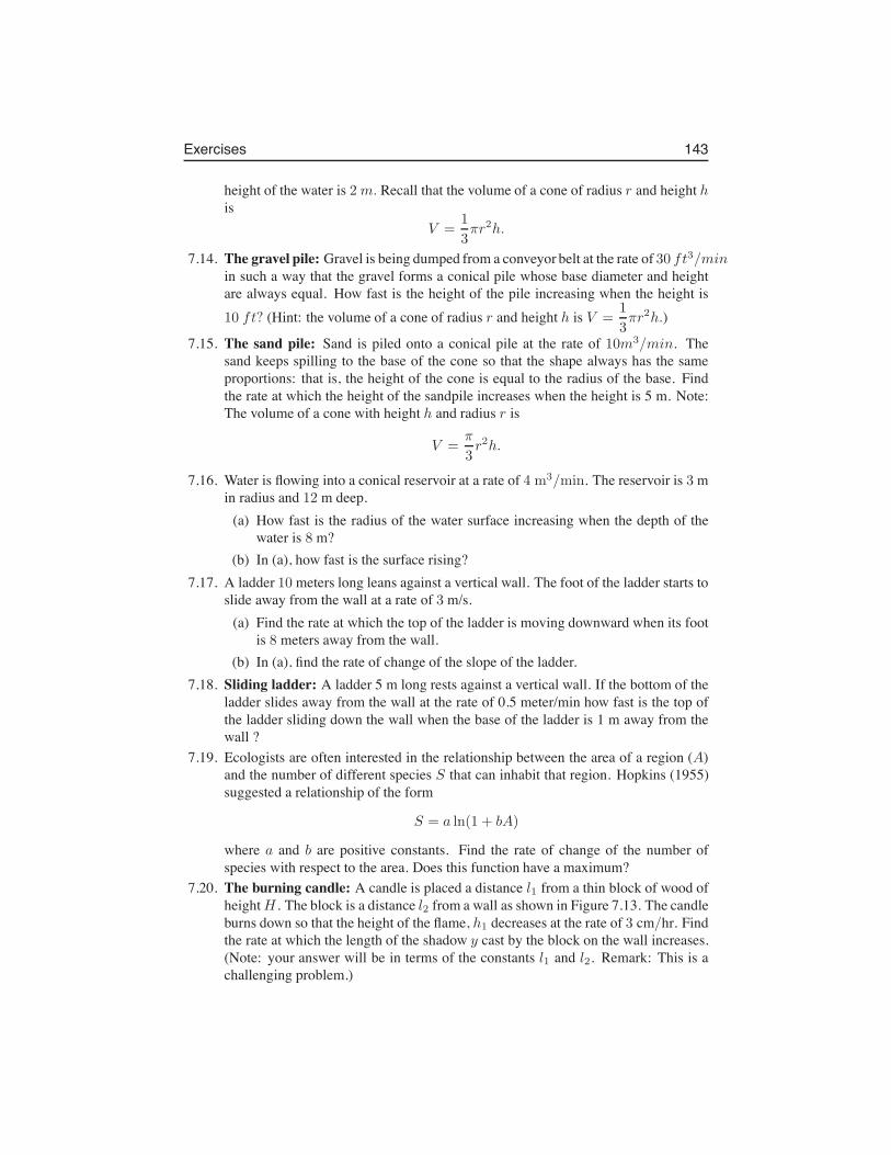
Exercises 143
height of the water is 2m. Recall that the volume of a cone of radius r and height his
V =1
3πr2h.
7.14. The gravel pile: Gravel is being dumped from a conveyor belt at the rate of 30 ft3/minin such a way that the gravel forms a conical pile whose base diameter and heightare always equal. How fast is the height of the pile increasing when the height is10 ft? (Hint: the volume of a cone of radius r and height h is V =
1
3πr2h.)
7.15. The sand pile: Sand is piled onto a conical pile at the rate of 10m3/min. Thesand keeps spilling to the base of the cone so that the shape always has the sameproportions: that is, the height of the cone is equal to the radius of the base. Findthe rate at which the height of the sandpile increases when the height is 5 m. Note:The volume of a cone with height h and radius r is
V =π
3r2h.
7.16. Water is flowing into a conical reservoir at a rate of 4 m3/min. The reservoir is 3 min radius and 12 m deep.
(a) How fast is the radius of the water surface increasing when the depth of thewater is 8 m?
(b) In (a), how fast is the surface rising?7.17. A ladder 10 meters long leans against a vertical wall. The foot of the ladder starts to
slide away from the wall at a rate of 3 m/s.(a) Find the rate at which the top of the ladder is moving downward when its foot
is 8 meters away from the wall.(b) In (a), find the rate of change of the slope of the ladder.
7.18. Sliding ladder: A ladder 5 m long rests against a vertical wall. If the bottom of theladder slides away from the wall at the rate of 0.5 meter/min how fast is the top ofthe ladder sliding down the wall when the base of the ladder is 1 m away from thewall ?
7.19. Ecologists are often interested in the relationship between the area of a region (A)and the number of different species S that can inhabit that region. Hopkins (1955)suggested a relationship of the form
S = a ln(1 + bA)
where a and b are positive constants. Find the rate of change of the number ofspecies with respect to the area. Does this function have a maximum?
7.20. The burning candle: A candle is placed a distance l1 from a thin block of wood ofheight H . The block is a distance l2 from a wall as shown in Figure 7.13. The candleburns down so that the height of the flame, h1 decreases at the rate of 3 cm/hr. Findthe rate at which the length of the shadow y cast by the block on the wall increases.(Note: your answer will be in terms of the constants l1 and l2. Remark: This is achallenging problem.)
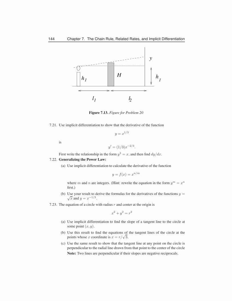
144 Chapter 7. The Chain Rule, Related Rates, and Implicit Differentiation
l l
Hh h
1
1 1
y
2
Figure 7.13. Figure for Problem 20
7.21. Use implicit differentiation to show that the derivative of the function
y = x1/3
isy′ = (1/3)x−2/3.
First write the relationship in the form y3 = x, and then find dy/dx.7.22. Generalizing the Power Law:
(a) Use implicit differentiation to calculate the derivative of the function
y = f(x) = xn/m
where m and n are integers. (Hint: rewrite the equation in the form ym = xn
first.)(b) Use your result to derive the formulas for the derivatives of the functions y =√
x and y = x−1/3.7.23. The equation of a circle with radius r and center at the origin is
x2 + y2 = r2
(a) Use implicit differentiation to find the slope of a tangent line to the circle atsome point (x, y).
(b) Use this result to find the equations of the tangent lines of the circle at thepoints whose x coordinate is x = r/
√3.
(c) Use the same result to show that the tangent line at any point on the circle isperpendicular to the radial line drawn from that point to the center of the circleNote: Two lines are perpendicular if their slopes are negative reciprocals.
Exercises 145
7.24. The equation of a circle with radius 5 and center at (1, 1) is
(x− 1)2 + (y − 1)2 = 25
(a) Find the slope of the tangent line to this curve at the point (4, 5).(b) Find the equation of the tangent line.
7.25. Tangent to a hyperbola: The curve
x2 − y2 = 1
is a hyperbola. Use implicit differentiation to show that for large x and y values, theslope dy/dx of the curve is approximately 1.
7.26. An ellipse: Use implicit differentiation to find the points on the ellipse
x2
4+
y2
9= 1
at which the slope is -1/2.7.27. Motion of a cell: In the study of cell motility, biologists often investigate a type of
cell called a keratocyte, an epidermal cell that is found in the scales of fish. Thisflat, elliptical cell crawls on a flat surface, and is known to be important in healingwounds. The 2D outline of the cell can be approximated by the ellipse
x2/100 + y2/25 = 1
where x and y are distances in µ (Note: 1 micron is 10−6 meters). When the motionof the cell is filmed, it is seen that points on the “leading edge” (top arc of the ellipse)move in a direction perpendicular to the edge. Determine the direction of motion ofthe point (xp, yp) on the leading edge.
7.28. Shortest path from nest to food sources:(a) Use the first derivative test to verify that the value x = d√
3is a local minimum
of the function L(x) given by Eqn (7.1)(b) Show that the shortest path is L = D +
√3d.
(c) In Section 7.7 we assumed that d << D, so that the food sources were closetogether relative to the distance from the nest. Now suppose that D = d/2.How would this change the solution to the problem?
7.29. Geometry of the shortest ants’ path: Use the results of Section 7.7 to show that inthe shortest path, the angles between the branches of the Y-shaped path are all 120◦,You may find it helpful to recall that sin(30) = 1/2, sin(60) =
√3/2.
7.30. The Folium of Descartes: A famous curve (see Figure 7.14) that was studied his-torically by many mathematicians (including Descartes) is
x3 + y3 = 3axy
You may assume that a is a positive constant.
Leah Keshet
Leah Keshet
Leah Keshet
degrees
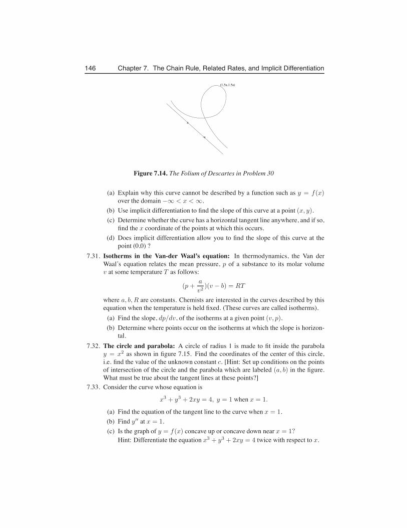
146 Chapter 7. The Chain Rule, Related Rates, and Implicit Differentiation
a
-a
(1.5a,1.5a)
Figure 7.14. The Folium of Descartes in Problem 30
(a) Explain why this curve cannot be described by a function such as y = f(x)over the domain −∞ < x < ∞.
(b) Use implicit differentiation to find the slope of this curve at a point (x, y).(c) Determine whether the curve has a horizontal tangent line anywhere, and if so,
find the x coordinate of the points at which this occurs.(d) Does implicit differentiation allow you to find the slope of this curve at the
point (0,0) ?7.31. Isotherms in the Van-der Waal’s equation: In thermodynamics, the Van der
Waal’s equation relates the mean pressure, p of a substance to its molar volumev at some temperature T as follows:
(p+a
v2)(v − b) = RT
where a, b, R are constants. Chemists are interested in the curves described by thisequation when the temperature is held fixed. (These curves are called isotherms).
(a) Find the slope, dp/dv, of the isotherms at a given point (v, p).(b) Determine where points occur on the isotherms at which the slope is horizon-
tal.7.32. The circle and parabola: A circle of radius 1 is made to fit inside the parabola
y = x2 as shown in figure 7.15. Find the coordinates of the center of this circle,i.e. find the value of the unknown constant c. [Hint: Set up conditions on the pointsof intersection of the circle and the parabola which are labeled (a, b) in the figure.What must be true about the tangent lines at these points?]
7.33. Consider the curve whose equation is
x3 + y3 + 2xy = 4, y = 1 when x = 1.
(a) Find the equation of the tangent line to the curve when x = 1.(b) Find y′′ at x = 1.(c) Is the graph of y = f(x) concave up or concave down near x = 1?
Hint: Differentiate the equation x3 + y3 + 2xy = 4 twice with respect to x.
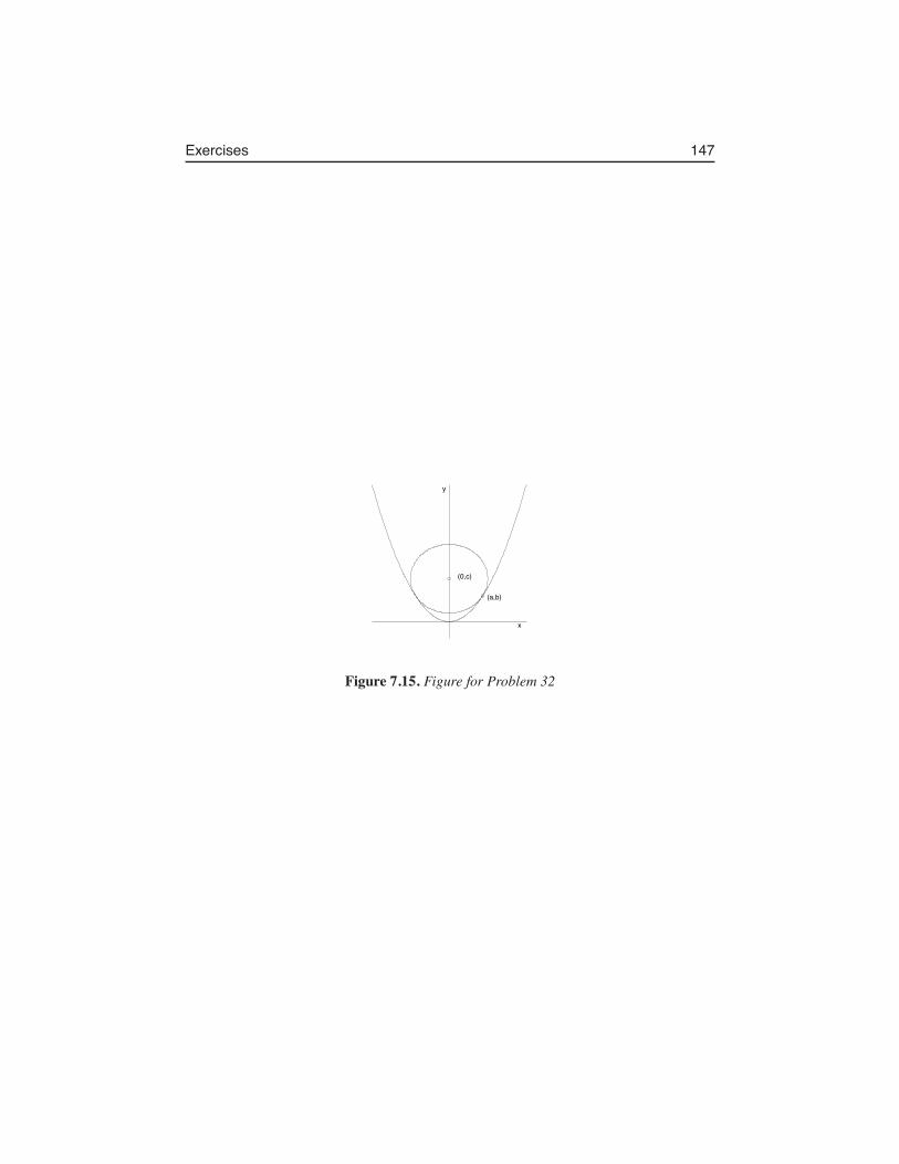
Exercises 147
x
y
(0,c)
(a,b)
Figure 7.15. Figure for Problem 32

148 Chapter 7. The Chain Rule, Related Rates, and Implicit Differentiation
Chapter 8
Exponential functions
8.1 The Andromeda Strain”The mathematics of uncontrolled growth are frightening. A single cell of the bacterium E.coli would, under ideal circumstances, divide every twenty minutes. That is not particularlydisturbing until you think about it, but the fact is that bacteria multiply geometrically: onebecomes two, two become four, four become eight, and so on. In this way it can be shownthat in a single day, one cell of E. coli could produce a super-colony equal in size andweight to the entire planet Earth.”
Michael Crichton (1969) The Andromeda Strain, Dell, N.Y. p247
The Andromeda Strain scenario motivates our investigation of a new family of functionsthat represent exponential growth. We start with values of the form 2n where n = 1, 2 . . .is an integer. To get a sense of how 2n grows with n, we list the first such values (n =1, . . . , 10) in Table 8.1. It is clear that an initially “gentle” growth becomes extremelysteep in just a few steps.
Our goal in this chapter is to generalize the discrete pattern of numbers in this tableto a continuous function 2x where x need not be an integer. We investigate how the base ofthe exponential function ax, where a > 0 is arbitrary affects the pattern. Once a continuousfunction is defined, we can attach a meaning to the idea of its derivative. Computing thederivative of an exponential function, we encounter a specially convenient base denoted e,and then inestigate the exponential function ex.
On the way to this goal, we also check the claim made by Michael Crichton aboutthe rapid growth of a bacterial colony.
Example 8.1 (Growth of E. coli:) Use the following facts to check the assertion made byMichael Crichton in the quotation at the beginning of this chapter.
• Mass of 1 E. coli cell : 1 nanogram = 10−9gm = 10−12kg.
• Mass of Planet Earth : 6 · 1024 kg
149
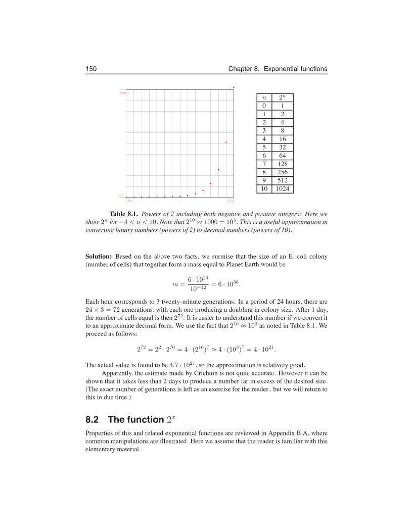
150 Chapter 8. Exponential functions
-4.0 10.00.0
1000.0n 2n
0 11 22 43 84 165 326 647 1288 2569 512
10 1024
Table 8.1. Powers of 2 including both negative and positive integers: Here weshow 2n for −4 < n < 10. Note that 210 ≈ 1000 = 103. This is a useful approximation inconverting binary numbers (powers of 2) to decimal numbers (powers of 10).
Solution: Based on the above two facts, we surmise that the size of an E. coli colony(number of cells) that together form a mass equal to Planet Earth would be
m =6 · 1024
10−12= 6 · 1036.
Each hour corresponds to 3 twenty-minute generations. In a period of 24 hours, there are24× 3 = 72 generations, with each one producing a doubling in colony size. After 1 day,the number of cells equal is then 272. It is easier to understand this number if we convert itto an approximate decimal form. We use the fact that 210 ≈ 103 as noted in Table 8.1. Weproceed as follows:
272 = 22 · 270 = 4 · (210)7 ≈ 4 · (103)7 = 4 · 1021.
The actual value is found to be 4.7 · 1021, so the approximation is relatively good.Apparently, the estimate made by Crichton is not quite accurate. However it can be
shown that it takes less than 2 days to produce a number far in excess of the desired size.(The exact number of generations is left as an exercise for the reader.. but we will return tothis in due time.)
8.2 The function 2x
Properties of this and related exponential functions are reviewed in Appendix B.A, wherecommon manipulations are illustrated. Here we assume that the reader is familiar with thiselementary material.
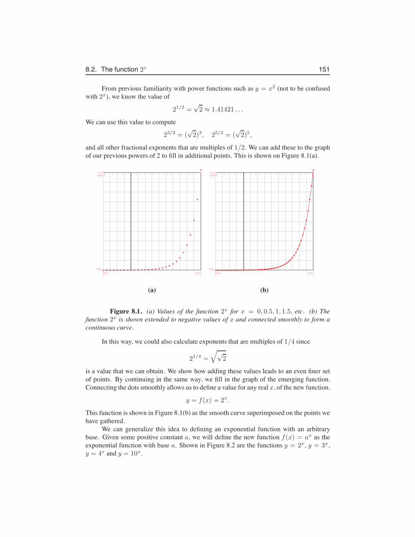
8.2. The function 2x 151
From previous familiarity with power functions such as y = x2 (not to be confusedwith 2x), we know the value of
21/2 =√2 ≈ 1.41421 . . .
We can use this value to compute
23/2 = (√2)3, 25/2 = (
√2)5,
and all other fractional exponents that are multiples of 1/2. We can add these to the graphof our previous powers of 2 to fill in additional points. This is shown on Figure 8.1(a).
-4.0 10.00.0
1000.0
-4.0 10.00.0
1000.0
(a) (b)
Figure 8.1. (a) Values of the function 2x for x = 0, 0.5, 1, 1.5, etc. (b) Thefunction 2x is shown extended to negative values of x and connected smoothly to form acontinuous curve.
In this way, we could also calculate exponents that are multiples of 1/4 since
21/4 =
√√2
is a value that we can obtain. We show how adding these values leads to an even finer setof points. By continuing in the same way, we fill in the graph of the emerging function.Connecting the dots smoothly allows us to define a value for any real x, of the new function,
y = f(x) = 2x.
This function is shown in Figure 8.1(b) as the smooth curve superimposed on the points wehave gathered.
We can generalize this idea to defining an exponential function with an arbitrarybase. Given some positive constant a, we will define the new function f(x) = ax as theexponential function with base a. Shown in Figure 8.2 are the functions y = 2x, y = 3x,y = 4x and y = 10x.
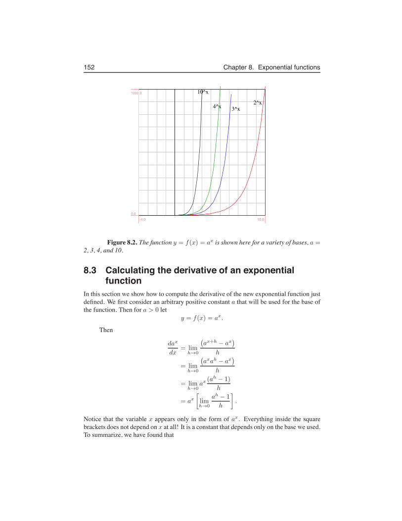
152 Chapter 8. Exponential functions
10^x
4^x 3^x2^x
-4.0 10.00.0
1000.0
Figure 8.2. The function y = f(x) = ax is shown here for a variety of bases, a =2, 3, 4, and 10.
8.3 Calculating the derivative of an exponentialfunction
In this section we show how to compute the derivative of the new exponential function justdefined. We first consider an arbitrary positive constant a that will be used for the base ofthe function. Then for a > 0 let
y = f(x) = ax.
Then
dax
dx= lim
h→0
(
ax+h − ax)
h
= limh→0
(
axah − ax)
h
= limh→0
ax(ah − 1)
h
= ax[
limh→0
ah − 1
h
]
.
Notice that the variable x appears only in the form of ax. Everything inside the squarebrackets does not depend on x at all! It is a constant that depends only on the base we used.To summarize, we have found that
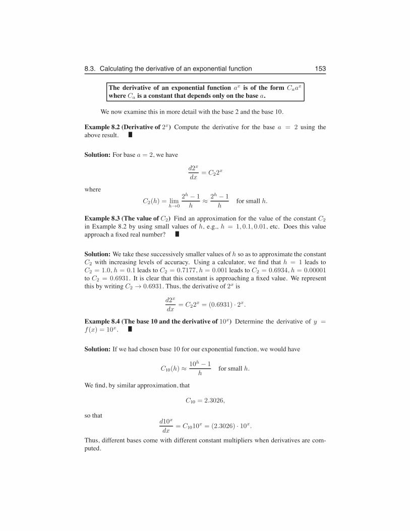
8.3. Calculating the derivative of an exponential function 153
The derivative of an exponential function ax is of the form Caax
where Ca is a constant that depends only on the base a.
We now examine this in more detail with the base 2 and the base 10.
Example 8.2 (Derivative of 2x) Compute the derivative for the base a = 2 using theabove result.
Solution: For base a = 2, we have
d2x
dx= C22
x
where
C2(h) = limh→0
2h − 1
h≈
2h − 1
hfor small h.
Example 8.3 (The value of C2) Find an approximation for the value of the constant C2
in Example 8.2 by using small values of h, e.g., h = 1, 0.1, 0.01, etc. Does this valueapproach a fixed real number?
Solution: We take these successively smaller values of h so as to approximate the constantC2 with increasing levels of accuracy. Using a calculator, we find that h = 1 leads toC2 = 1.0, h = 0.1 leads to C2 = 0.7177, h = 0.001 leads to C2 = 0.6934, h = 0.00001to C2 = 0.6931. It is clear that this constant is approaching a fixed value. We representthis by writing C2 → 0.6931. Thus, the derivative of 2x is
d2x
dx= C22
x = (0.6931) · 2x.
Example 8.4 (The base 10 and the derivative of 10x) Determine the derivative of y =f(x) = 10x.
Solution: If we had chosen base 10 for our exponential function, we would have
C10(h) ≈10h − 1
hfor small h.
We find, by similar approximation, that
C10 = 2.3026,
so thatd10x
dx= C1010
x = (2.3026) · 10x.
Thus, different bases come with different constant multipliers when derivatives are com-puted.
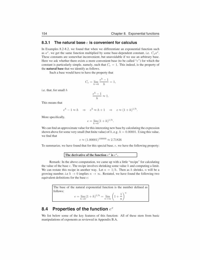
154 Chapter 8. Exponential functions
8.3.1 The natural base e is convenient for calculusIn Examples 8.2-8.2, we found that when we differentiate an exponential function suchas ax, we get the same function multiplied by some base-dependent constant, i.e. Caax.These constants are somewhat inconvenient, but unavoidable if we use an arbitrary base.Here we ask whether there exists a more convenient base (to be called “e”) for which theconstant is particularly simple, namely, such that Ce = 1. This indeed, is the property ofthe natural base that we identify as follows.
Such a base would have to have the property that
Ce = limh→0
eh − 1
h= 1,
i.e. that, for small heh − 1
h≈ 1.
This means that
eh − 1 ≈ h ⇒ eh ≈ h+ 1 ⇒ e ≈ (1 + h)1/h.
More specifically,e = lim
h→0(1 + h)1/h.
We can find an approximate value for this interesting new base by calculating the expressionshown above for some very small (but finite value) of h, e.g. h = 0.00001. Using this value,we find that
e ≈ (1.00001)100000 ≈ 2.71826
To summarize, we have found that for this special base, e, we have the following property:
The derivative of the function ex is ex.
Remark: In the above computation, we came up with a little “recipe” for calculatingthe value of the base e. The recipe involves shrinking some value h and computing a limit.We can restate this recipe in another way. Let n = 1/h. Then as h shrinks, n will be agrowing number, i.e h → 0 implies n → ∞. Restated, we have found the following twoequivalent definitions for the base e:
The base of the natural exponential function is the number defined asfollows:
e = limh→0
(1 + h)1/h = limn→∞
(
1 +1
n
)n
8.4 Properties of the function ex
We list below some of the key features of this function: All of these stem from basicmanipulations of exponents as reviewed in Appendix B.A.
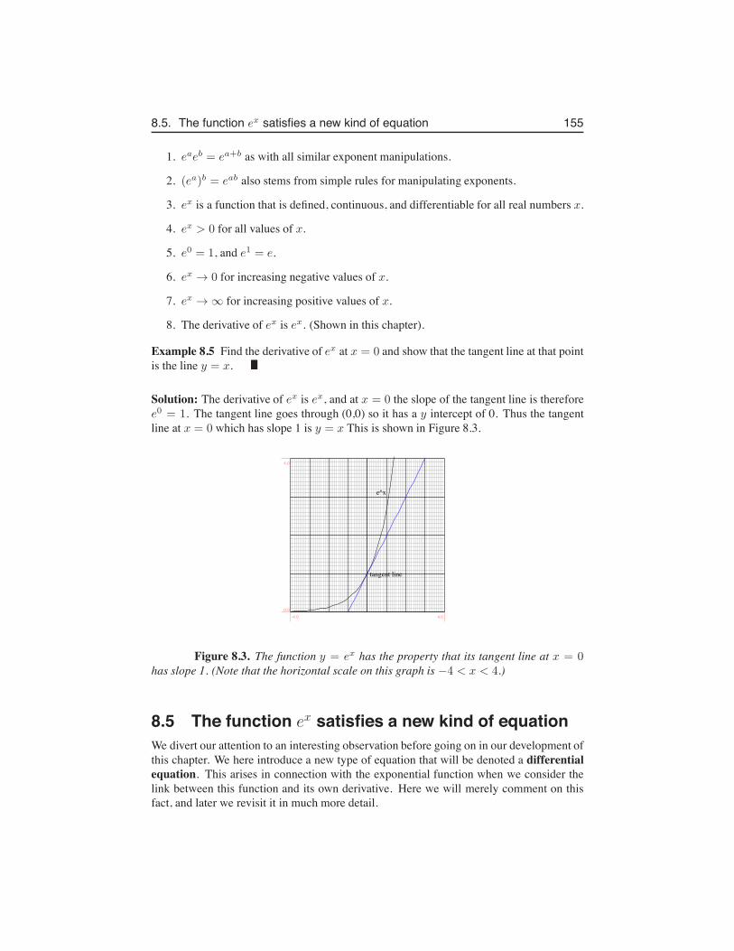
8.5. The function ex satisfies a new kind of equation 155
1. eaeb = ea+b as with all similar exponent manipulations.
2. (ea)b = eab also stems from simple rules for manipulating exponents.
3. ex is a function that is defined, continuous, and differentiable for all real numbers x.
4. ex > 0 for all values of x.
5. e0 = 1, and e1 = e.
6. ex → 0 for increasing negative values of x.
7. ex → ∞ for increasing positive values of x.
8. The derivative of ex is ex. (Shown in this chapter).
Example 8.5 Find the derivative of ex at x = 0 and show that the tangent line at that pointis the line y = x.
Solution: The derivative of ex is ex, and at x = 0 the slope of the tangent line is thereforee0 = 1. The tangent line goes through (0,0) so it has a y intercept of 0. Thus the tangentline at x = 0 which has slope 1 is y = x This is shown in Figure 8.3.
e^x
tangent line
-4.0 4.00.0
4.0
Figure 8.3. The function y = ex has the property that its tangent line at x = 0has slope 1. (Note that the horizontal scale on this graph is −4 < x < 4.)
8.5 The function ex satisfies a new kind of equationWe divert our attention to an interesting observation before going on in our development ofthis chapter. We here introduce a new type of equation that will be denoted a differentialequation. This arises in connection with the exponential function when we consider thelink between this function and its own derivative. Here we will merely comment on thisfact, and later we revisit it in much more detail.
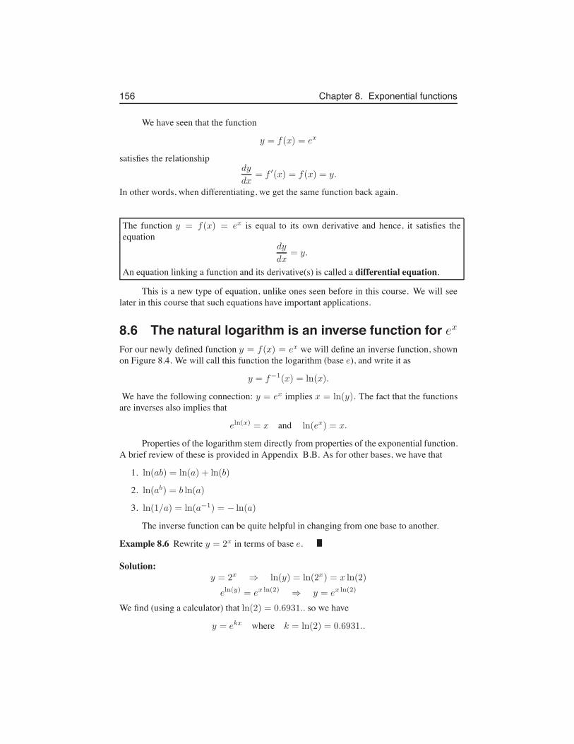
156 Chapter 8. Exponential functions
We have seen that the function
y = f(x) = ex
satisfies the relationshipdy
dx= f ′(x) = f(x) = y.
In other words, when differentiating, we get the same function back again.
The function y = f(x) = ex is equal to its own derivative and hence, it satisfies theequation
dy
dx= y.
An equation linking a function and its derivative(s) is called a differential equation.
This is a new type of equation, unlike ones seen before in this course. We will seelater in this course that such equations have important applications.
8.6 The natural logarithm is an inverse function for exFor our newly defined function y = f(x) = ex we will define an inverse function, shownon Figure 8.4. We will call this function the logarithm (base e), and write it as
y = f−1(x) = ln(x).
We have the following connection: y = ex implies x = ln(y). The fact that the functionsare inverses also implies that
eln(x) = x and ln(ex) = x.
Properties of the logarithm stem directly from properties of the exponential function.A brief review of these is provided in Appendix B.B. As for other bases, we have that
1. ln(ab) = ln(a) + ln(b)
2. ln(ab) = b ln(a)
3. ln(1/a) = ln(a−1) = − ln(a)
The inverse function can be quite helpful in changing from one base to another.
Example 8.6 Rewrite y = 2x in terms of base e.
Solution:y = 2x ⇒ ln(y) = ln(2x) = x ln(2)
eln(y) = ex ln(2) ⇒ y = ex ln(2)
We find (using a calculator) that ln(2) = 0.6931.. so we have
y = ekx where k = ln(2) = 0.6931..
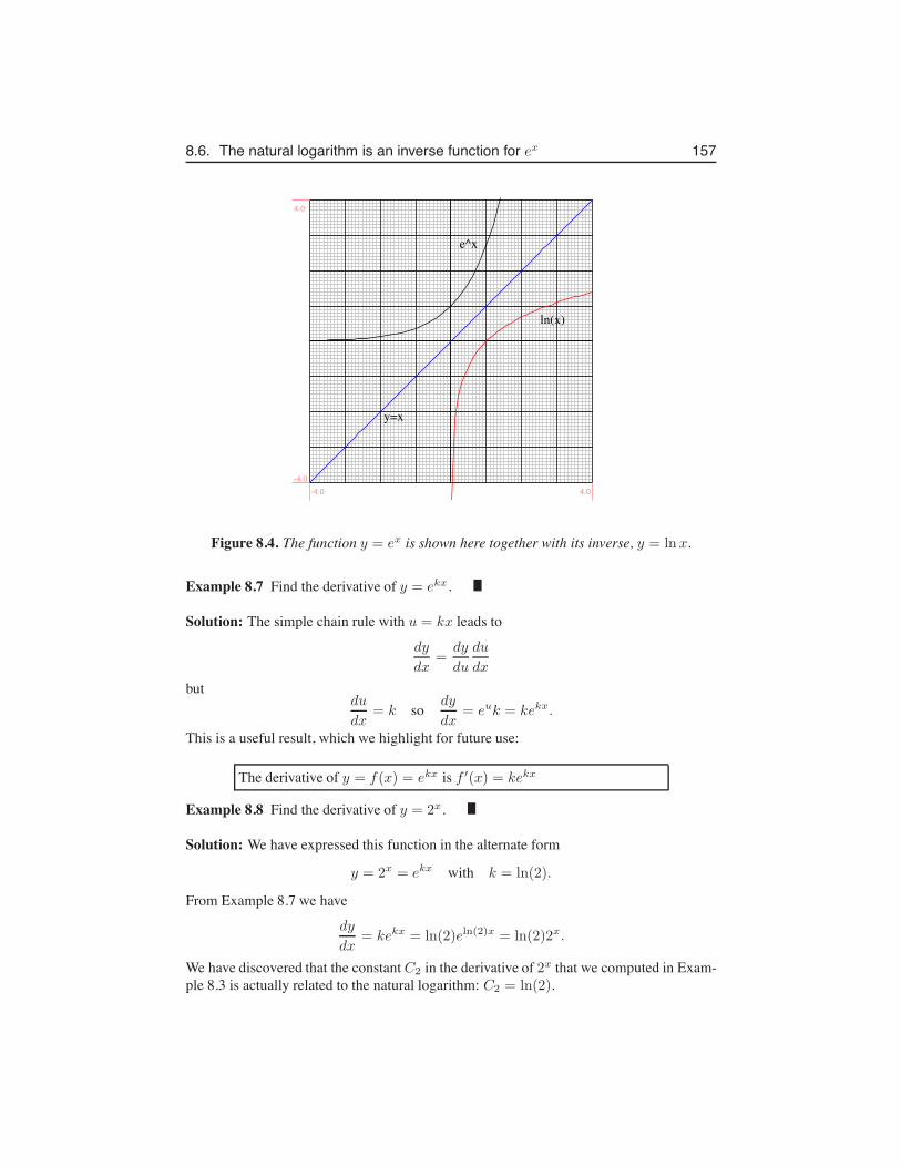
8.6. The natural logarithm is an inverse function for ex 157
e^x
ln(x)
y=x
-4.0 4.0-4.0
4.0
Figure 8.4. The function y = ex is shown here together with its inverse, y = lnx.
Example 8.7 Find the derivative of y = ekx.
Solution: The simple chain rule with u = kx leads to
dy
dx=
dy
du
du
dx
butdu
dx= k so dy
dx= euk = kekx.
This is a useful result, which we highlight for future use:
The derivative of y = f(x) = ekx is f ′(x) = kekx
Example 8.8 Find the derivative of y = 2x.
Solution: We have expressed this function in the alternate form
y = 2x = ekx with k = ln(2).
From Example 8.7 we have
dy
dx= kekx = ln(2)eln(2)x = ln(2)2x.
We have discovered that the constant C2 in the derivative of 2x that we computed in Exam-ple 8.3 is actually related to the natural logarithm: C2 = ln(2).
158 Chapter 8. Exponential functions
8.7 How many bacteriaWe can now return to our Andromeda strain and answer a question we had left unanswered:How long will it take for the population to attain a size of 6 · 1036 cells, i.e. to grow to anEarth-sized colony.
We recall that the doubling time for the bacteria is 20 min, so that one generation (orone doubling occurs for every multiple of t/20). However, it is not necessarily true that allcells will split in a synchronized way. This means that after t minutes, we expect that thenumber, B(t) of bacteria would be roughly given by the smooth function:
B(t) = 2t/20.
(Note that this function agrees with our previous table and graph for powers of 2 at allinteger multiples of the generation time, i.e. for t = 20, 40, 60, 80.. minutes.)
Example 8.9 How long will it take to reach size B = 6 · 1036?
Solution: We can compute this as follows:
6 · 1036 = 2t/20 ⇒ ln(6 · 1036) = ln(2t/20)
ln(6) + 36 ln(10) =t
20ln(2)
so
t = 20ln(6) + 36 ln(10)
ln(2)= 20
1.79 + 36(2.3)
0.693= 2441.27
This is the time in minutes. In hours, it would take 2441.27/60 = 40.68 hours for the colonyto grow to such a size.
Example 8.10 (Using base e:) Express the number of bacteria in terms of base e (for prac-tice with base conversions).
Solution: We would do this as follows:
B(t) = 2t/20 ⇒ ln(B) =t
20ln(2)
eln(B(t)) = et20
ln(2) ⇒ B(t) = ekt where k =ln(2)
20.
The constant k will be referred to as the growth rate of the bacteria. We observe that thisconstant can be written as:
k =ln(2)
doubling time.
We will see the usefulness of this approach very soon.
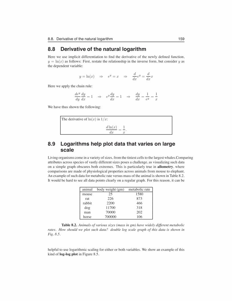
8.8. Derivative of the natural logarithm 159
8.8 Derivative of the natural logarithmHere we use implicit differentiation to find the derivative of the newly defined function,y = ln(x) as follows: First, restate the relationship in the inverse form, but consider y asthe dependent variable:
y = ln(x) ⇒ ey = x ⇒d
dxey =
d
dxx
Here we apply the chain rule:
dey
dy
dy
dx= 1 ⇒ ey
dy
dx= 1 ⇒
dy
dx=
1
ey=
1
x
We have thus shown the following:
The derivative of ln(x) is 1/x:
d ln(x)
dx=
1
x.
8.9 Logarithms help plot data that varies on largescale
Living organisms come in a variety of sizes, from the tiniest cells to the largest whales.Comparingattributes across species of vastly different sizes poses a challenge, as visualizing such dataon a simple graph obscures both extremes. This is particularly true in allometry, wherecomparisons are made of physiological properties across animals from mouse to elephant.An example of such data for metabolic rate versus mass of the animal is shown in Table 8.2.It would be hard to see all data points clearly on a regular graph. For this reason, it can be
animal body weight (gm) metabolic ratemouse 25 1580
rat 226 873rabbit 2200 466dog 11700 318man 70000 202horse 700000 106
Table 8.2. Animals of various sizes (mass in gm) have widely different metabolicrates. How should we plot such data? double log scale graph of this data is shown inFig. 8.5.
helpful to use logarithmic scaling for either or both variables. We show an example of thiskind of log-log plot in Figure 8.5.
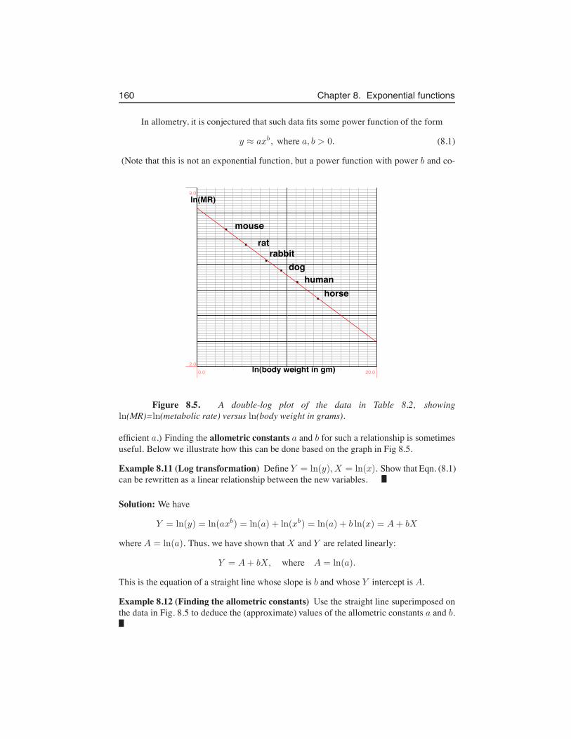
160 Chapter 8. Exponential functions
In allometry, it is conjectured that such data fits some power function of the form
y ≈ axb, where a, b > 0. (8.1)
(Note that this is not an exponential function, but a power function with power b and co-
ln(body weight in gm)
ln(MR)
mouse
ratrabbit
doghuman
horse
0.0 20.02.0
9.0
Figure 8.5. A double-log plot of the data in Table 8.2, showingln(MR)=ln(metabolic rate) versus ln(body weight in grams).
efficient a.) Finding the allometric constants a and b for such a relationship is sometimesuseful. Below we illustrate how this can be done based on the graph in Fig 8.5.
Example 8.11 (Log transformation) Define Y = ln(y), X = ln(x). Show that Eqn. (8.1)can be rewritten as a linear relationship between the new variables.
Solution: We have
Y = ln(y) = ln(axb) = ln(a) + ln(xb) = ln(a) + b ln(x) = A+ bX
where A = ln(a). Thus, we have shown that X and Y are related linearly:
Y = A+ bX, where A = ln(a).
This is the equation of a straight line whose slope is b and whose Y intercept is A.
Example 8.12 (Finding the allometric constants) Use the straight line superimposed onthe data in Fig. 8.5 to deduce the (approximate) values of the allometric constants a and b.
8.10. Additional problems 161
Solution: We use the straight line that has been fitted to the data in Fig. 8.5. The Y interceptof this line is roughly 8.2. The line goes through the points (20,3) and (0,8.2) so its slopeis ≈ (3− 8.2)/20 = −0.26. According to the relationship we found in Example 8.11,
8.2 = A = ln(a) ⇒ a = e8.2 = 3640, and b = −0.26.
Thus, reverting to the original allometric relationship leads to
y = axb = 3640x−0.26 =3640
x0.26.
It is clear that the metabolic rate y decreases with the size x of the animal, as indicated bythe data in Table 8.2.
8.10 Additional problems8.10.1 Chemical reactionsAccording to the collision theory of bimolecular gas reactions, a reaction between twomolecules occurs when the molecules collide with energy greater than some activationenergy, Ea, referred to as the Arrhenius activation energy. We will assume that Ea > 0is constant for the given substance. The fraction of bimolecular reactions in which thiscollision energy is achieved is
F = e−(Ea/RT )
where T is temperature (in degrees Kelvin) and R > 0 is the gas constant.
Example 8.13 Suppose that the temperature T increases at some constant rate C per unittime. Determine the rate of change of the fraction F of collisions that result in a successfulreaction.
Solution: We are givenF = e−(Ea/RT )
anddT
dt= C.
Let u = −Ea/RT then F = eu, We use the chain rule to calculate:
dF
dt=
dF
du
du
dT
dT
dt.
Further, we havedF
du= eu and du
dT=
Ea
RT 2.
Assembling these parts, we have
dF
dt= eu
Ea
RT 2C = C
Ea
RT−2e−(Ea/RT ).
162 Chapter 8. Exponential functions
Exercises8.1. Graph the following functions:
(a) f(x) = x2e−x
(b) f(x) = ln(x2 + 3)
(c) f(x) = ln(e2x)
8.2. Express the following in terms of base e:(a) y = 3x
(b) y = 17x
(c) y = 15x2+2
Express the following in terms of base 2:(d) y = 9x
(e) y = 8x
(f) y = −ex2+3
Express the following in terms of base 10:(g) y = 21x
(h) y = 1000−10x
(i) y = 50x2−1
8.3. Compare the values of each pair of numbers (i.e. indicate which is larger):(a) 50.75, 50.65
(b) 0.4−0.2, 0.40.2
(c) 1.0012, 1.0013
(d) 0.9991.5, 0.9992.3
8.4. Rewrite each of the following equations in logarithmic form:(a) 34 = 81
(b) 3−2 = 19
(c) 27−13 =
1
38.5. Solve the following equations for x:
(a) lnx = 2 lna+ 3 ln b
(b) loga x = loga b− 23 loga c
8.6. Reflections and transformations: What is the relationship between the graph ofy = 3x and the graph of each of the following functions?
(a) y = −3x (b) y = 3−x (c) y = 31−x
(d) y = 3|x| (e) y = 2 · 3x (e) y = log3 x
8.7. Solve the following equations for x:
Exercises 163
(a) e3−2x = 5
(b) ln(3x− 1) = 4
(c) ln(ln(x)) = 2
(d) eax = Cebx, where a $= b and C > 0.8.8. Find the first derivative for each of the following functions:
(a) y = ln(2x+ 3)3
(b) y = ln3(2x+ 3)
(c) y = ln(cos 12x)
(d) y = loga(x3 − 2x) (Hint :
d
dx(loga x) =
1
x ln a)
(e) y = e3x2
(f) y = a−12x
(g) y = x3 · 2x
(h) y = eex
(i) y =et − e−t
et + e−t
8.9. Find the maximum and minimum points as well as all inflection points of the fol-lowing functions:
(a) f(x) = x(x2 − 4)
(b) f(x) = x3 − ln(x), x > 0
(c) f(x) = xe−x
(d) f(x) = 11−x + 1
1+x ,−1 < x < 1
(e) f(x) = x− 3 3√x
(f) f(x) = e−2x − e−x
8.10. Shown in Figure 10 is the graph of y = Cekt for some constants C, k, and a tangentline. Use data from the graph to determine C and k.
8.11. Consider the two functions(a) y1(t) = 10e−0.1t,(b) y2(t) = 10e0.1t.
Which one is decreasing and which one is increasing? In each case, find the valueof the function at t = 0. Find the time at which the increasing function has doubledfrom this initial value. Find the time at which the decreasing function has fallen tohalf of its initial value. [Remark: these values of t are called, the doubling time, andthe half-life, respectively]
8.12. Shannon Entropy: In a recent application of information theory to the field ofgenomics, a function called the Shannon entropy, H , was considered. A given geneis represented as a binary device: it can be either “on” or “off” (i.e. being expressed
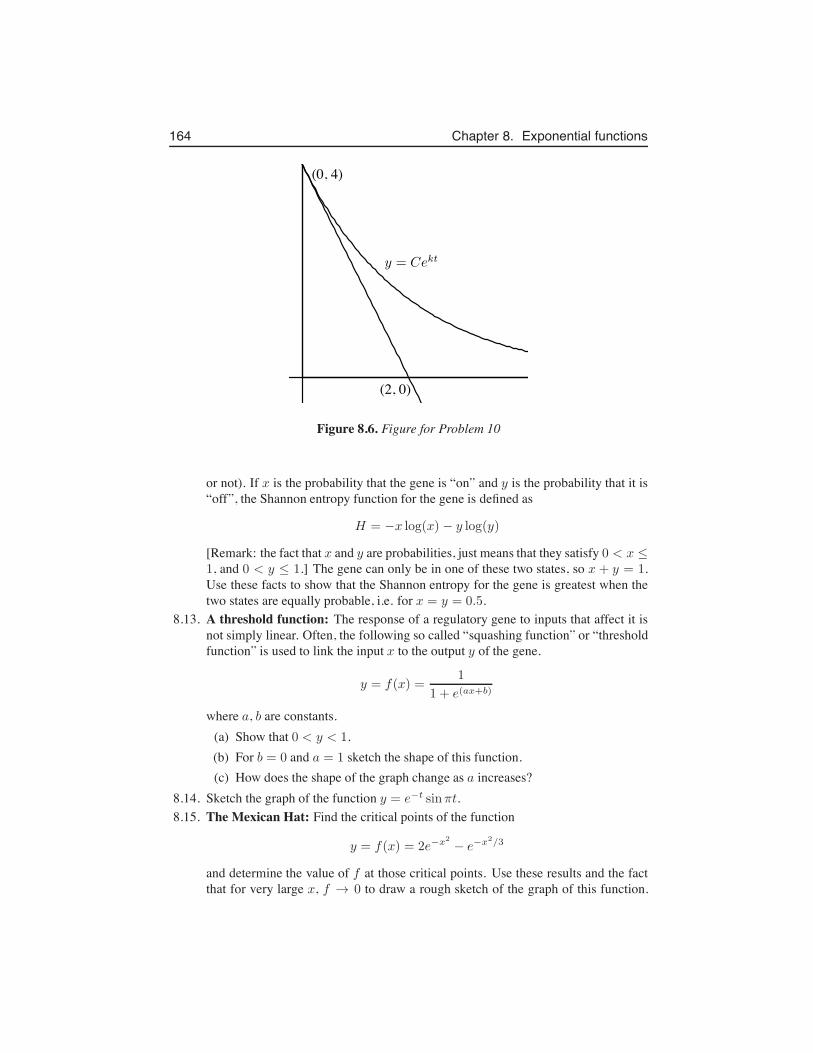
164 Chapter 8. Exponential functions
(0, 4)
(2, 0)
y = Cekt
Figure 8.6. Figure for Problem 10
or not). If x is the probability that the gene is “on” and y is the probability that it is“off”, the Shannon entropy function for the gene is defined as
H = −x log(x) − y log(y)
[Remark: the fact that x and y are probabilities, just means that they satisfy 0 < x ≤1, and 0 < y ≤ 1.] The gene can only be in one of these two states, so x + y = 1.Use these facts to show that the Shannon entropy for the gene is greatest when thetwo states are equally probable, i.e. for x = y = 0.5.
8.13. A threshold function: The response of a regulatory gene to inputs that affect it isnot simply linear. Often, the following so called “squashing function” or “thresholdfunction” is used to link the input x to the output y of the gene.
y = f(x) =1
1 + e(ax+b)
where a, b are constants.(a) Show that 0 < y < 1.(b) For b = 0 and a = 1 sketch the shape of this function.(c) How does the shape of the graph change as a increases?
8.14. Sketch the graph of the function y = e−t sinπt.8.15. The Mexican Hat: Find the critical points of the function
y = f(x) = 2e−x2
− e−x2/3
and determine the value of f at those critical points. Use these results and the factthat for very large x, f → 0 to draw a rough sketch of the graph of this function.
Exercises 165
Comment on why this function might be called “a Mexican Hat”. (Note: The sec-ond derivative is not very informative here, and we will not ask you to use it fordetermining concavity in this example. However, you may wish to calculate it justfor practice with the chain rule.)
8.16. The Ricker Equation: In studying salmon populations, a model often used is theRicker equation which relates the size of a fish population this year, x to the expectedsize next year y. (Note that these populations do not change continuously, since allthe parents die before the eggs are hatched.) The Ricker equation is
y = αxe−βx
where α,β > 0. Find the value of the current population which maximizes thesalmon population next year according to this model.
8.17. Spacing in a fish school: Life in a social group has advantages and disadvantages:protection from predators is one advantage. Disadvantages include competition withothers for food or resources. Spacing of individuals in a school of fish or a flock ofbirds is determined by the mutual attraction and repulsion of neighbors from oneanother: each individual does not want to stray too far from others, nor get tooclose.Suppose that when two fish are at distance x > 0 from one another, they are attractedwith “force” Fa and repelled with “force” Fr given by:
Fa = Ae−x/a
Fr = Re−x/r
where A,R, a, r are positive constants. A,R are related to the magnitudes of theforces, and a, r to the spatial range of these effects.
(a) Show that at the distance x = a the first function has fallen to (1/e) times itsvalue at the origin. (Recall e ≈ 2.7.) For what value of x does the secondfunction fall to (1/e) times its value at the origin? Note that this is the reasonwhy a, r are called spatial ranges of the forces.
(b) It is generally assumed that R > A and r < a. Interpret what this meanabout the comparative effects of the forces and sketch a graph showing the twofunctions on the same set of axes.
(c) Find the distance at which the forces exactly balance. This is called the com-fortable distance for the two individuals.
(d) If either A or R changes so that the ratio R/A decreases, does the comfortabledistance increase or decrease? (Give reason.)
(e) Similarly comment on what happens to the comfortable distance if a increasesor r decreases.
8.18. Seed distribution: The density of seeds at a distance x from a parent tree is ob-served to be
D(x) = D0e−x2/a2
,
166 Chapter 8. Exponential functions
where a > 0, D0 > 0 are positive constants. Insects that eat these seeds tend tocongregate near the tree so that the fraction of seeds that get eaten is
F (x) = e−x2/b2
where b > 0. (Remark: These functions are called Gaussian or Normal distributions.The parameters a, b are related to the “width” of these bell-shaped curves.) Thenumber of seeds that survive (i.e. are produced and not eaten by insects) is
S(x) = D(x)(1 − F (x))
Determine the distance x from the tree at which the greatest number of seeds survive.8.19. Euler’s “e”: In 1748, Euler wrote a classic book on calculus (“Introductio in
Analysin Infinitorum”) in which he showed that the function ex could be writtenin an expanded form similar to an (infinitely long) polynomial:
ex = 1 + x+x2
1 · 2+
x3
1 · 2 · 3+ ...
Use as many terms as necessary to find an approximate value for the number e andfor 1/e to 5 decimal places. Remark: we will see later that such expansions, calledpower series, are central to approximations of many functions.
Chapter 9
Exponential Growth andDecay: DifferentialEquations
9.1 Observations about the exponential functionIn a previous chapter we made an observation about a special property of the exponentialfunction
y = f(x) = ex
namely, that it satisfies the relationship
dy
dx= ex = y.
In this way, we encountered an important new class of equations,
dy
dx= y.
We call this a differential equation because it connects (one or more) derivatives of afunction with the function itself.
In this chapter we will study the implications of the above observation. Since mostof the applications that we examine will be time-dependent processes, we will here use t(for time) as the independent variable.
Then we can make the following observations:
1. Let y be the function of time:y = f(t) = et.
Thendy
dt= et = y.
With this slight change of notation, we see that the function y = et satisfies thedifferential equation
dy
dt= y.
167
168 Chapter 9. Exponential Growth and Decay: Differential Equations
2. Now considery = ekt.
Then, using the chain rule, and setting u = kt, and y = eu we find that
dy
dt=
dy
du
du
dt= eu · k = kekt = ky.
So we see that the function y = ekt satisfies the differential equation
dy
dt= ky.
3. If instead we had the functiony = e−kt,
we could similarly show that the differential equation it satisfies is
dy
dt= −ky.
4. Now suppose we had a constant in front, e.g. we were interested in the function
y = 5ekt.
Then, by simple differentiation and rearrangement we have
dy
dt= 5
d
dtekt = 5(kekt) = k(5ekt) = ky.
So we see that this function with the constant in front also satisfies the differentialequation
dy
dt= ky.
5. The conclusion we reached in the previous step did not depend at all on the constantout front. Indeed, if we had started with a function of the form
y = Cekt,
where C is any constant, we would still have a function that satisfies the same differ-ential equation.
6. While we will not prove this here, it turns out that these are the only functions thatsatisfy this equation.
The differential equationdy
dt= ky (9.1)
has as its solution, the function
y = Cekt.. (9.2)
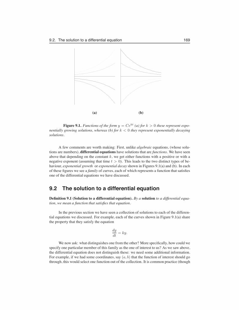
9.2. The solution to a differential equation 169
(a) (b)
Figure 9.1. Functions of the form y = Cekt (a) for k > 0 these represent expo-nentially growing solutions, whereas (b) for k < 0 they represent exponentially decayingsolutions.
A few comments are worth making: First, unlike algebraic equations, (whose solu-tions are numbers), differential equations have solutions that are functions. We have seenabove that depending on the constant k, we get either functions with a positive or with anegative exponent (assuming that time t > 0). This leads to the two distinct types of be-haviour, exponential growth or exponential decay shown in Figures 9.1(a) and (b). In eachof these figures we see a family of curves, each of which represents a function that satisfiesone of the differential equations we have discussed.
9.2 The solution to a differential equationDefinition 9.1 (Solution to a differential equation). By a solution to a differential equa-tion, we mean a function that satisfies that equation.
In the previous section we have seen a collection of solutions to each of the differen-tial equations we discussed. For example, each of the curves shown in Figure 9.1(a) sharethe property that they satisfy the equation
dy
dt= ky.
We now ask: what distinguishes one from the other? More specifically, how could wespecify one particular member of this family as the one of interest to us? As we saw above,the differential equation does not distinguish these: we need some additional information.For example, if we had some coordinates, say (a, b) that the function of interest should gothrough, this would select one function out of the collection. It is common practice (though
170 Chapter 9. Exponential Growth and Decay: Differential Equations
not essential) to specify the starting value or initial value of the function i.e. its value attime t = 0.
Definition 9.2 (Initial value). An initial value is the value at time t = 0 of the desiredsolution of a differential equation.
Example 9.3 Suppose we are given the differential equation (9.1) and the initial value
y(0) = y0
where y0 is some (known) fixed value. Find the value of the constant C in the solution(9.2).
Solution: We proceed as follows:
y(t) = Cekt, so y(0) = Cek·0 = Ce0 = C · 1 = C.
But, by the initial condition, y(0) = y0. So then,
C = y0
and we have established that
y(t) = y0ekt, where y0 is the initial value.
9.3 Where do differential equations come from?Figure 9.2 shows how differential equations arise in scientific investigations. The process ofgoing from initial vague observations about a system of interest (such as planetary motion)to a mathematical model, often involves a great deal of speculation, at first, about what ishappening, what causes the motion or the changes that take place, and what assumptionsmight be fruitful in trying to analyze and understand the system.
Once the cloud of doubt and vague ideas settles somewhat, and once the right sim-plifying assumptions are made, we often find that the mathematical model leads to a differ-ential equation. In most scientific applications, it may then be a huge struggle to figure outwhich functions would be the appropriate class of solutions to that differential equation,but if we can find those functions, we are in position to make quantitative predictions aboutthe system of interest.
In our case, we have stumbled on a simple differential equation by noticing a propertyof functions that we were already familiar with. This is a lucky accident, and we will exploitit in an application shortly.
In many cases, the process of modelling hardly stops when we have found the linkbetween the differential equation and solutions. Usually, we would then compare the pre-dictions to observations that may help us to refine the model, reject incorrect or inaccurateassumptions, or determine to what extent the model has limitations.
A simple example of population growth modelling is given as motivation for some ofthe ideas seen in this discussion.
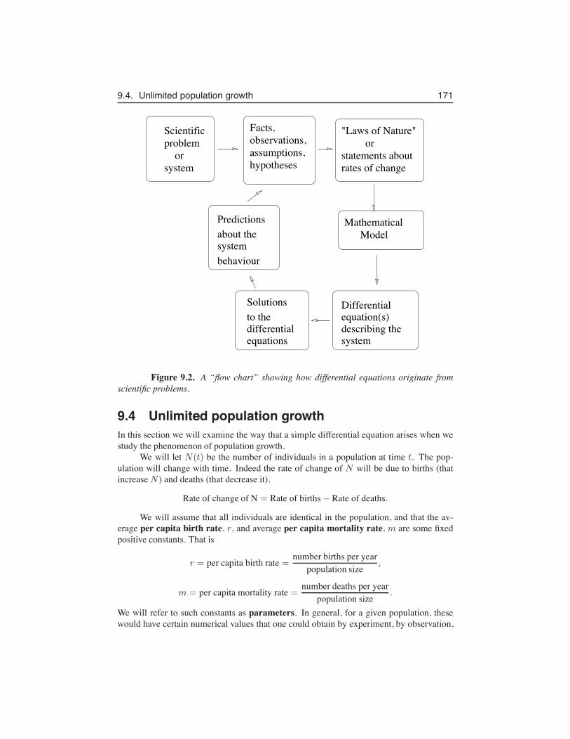
9.4. Unlimited population growth 171
Scientificproblem orsystem
Facts,observations,assumptions,hypotheses
"Laws of Nature" orstatements aboutrates of change
Mathematical
systemdescribing theequation(s)Differential
equationsdifferentialto theSolutions
Predictionsabout thesystem behaviour
Model
Figure 9.2. A “flow chart” showing how differential equations originate fromscientific problems.
9.4 Unlimited population growthIn this section we will examine the way that a simple differential equation arises when westudy the phenomenon of population growth.
We will let N(t) be the number of individuals in a population at time t. The pop-ulation will change with time. Indeed the rate of change of N will be due to births (thatincrease N ) and deaths (that decrease it).
Rate of change of N = Rate of births − Rate of deaths.
We will assume that all individuals are identical in the population, and that the av-erage per capita birth rate, r, and average per capita mortality rate, m are some fixedpositive constants. That is
r = per capita birth rate =number births per year
population size,
m = per capita mortality rate =number deaths per year
population size.
We will refer to such constants as parameters. In general, for a given population, thesewould have certain numerical values that one could obtain by experiment, by observation,
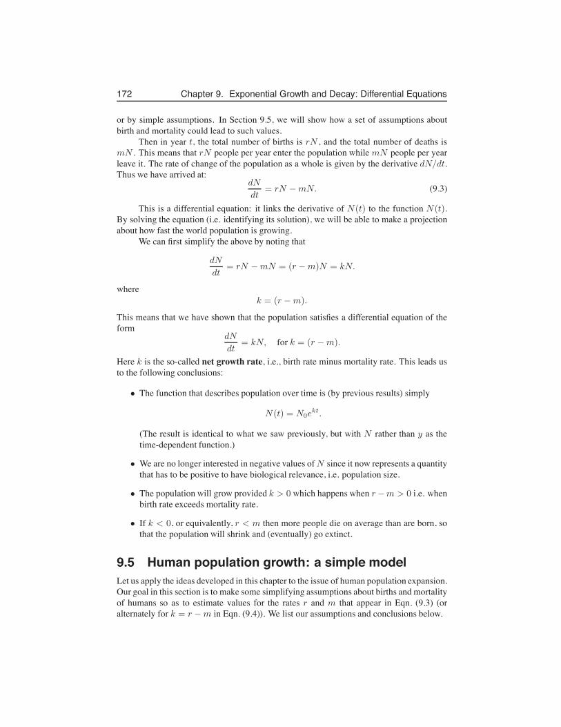
172 Chapter 9. Exponential Growth and Decay: Differential Equations
or by simple assumptions. In Section 9.5, we will show how a set of assumptions aboutbirth and mortality could lead to such values.
Then in year t, the total number of births is rN , and the total number of deaths ismN . This means that rN people per year enter the population while mN people per yearleave it. The rate of change of the population as a whole is given by the derivative dN/dt.Thus we have arrived at:
dN
dt= rN −mN. (9.3)
This is a differential equation: it links the derivative of N(t) to the function N(t).By solving the equation (i.e. identifying its solution), we will be able to make a projectionabout how fast the world population is growing.
We can first simplify the above by noting that
dN
dt= rN −mN = (r −m)N = kN.
wherek = (r −m).
This means that we have shown that the population satisfies a differential equation of theform
dN
dt= kN, for k = (r −m).
Here k is the so-called net growth rate, i.e., birth rate minus mortality rate. This leads usto the following conclusions:
• The function that describes population over time is (by previous results) simply
N(t) = N0ekt.
(The result is identical to what we saw previously, but with N rather than y as thetime-dependent function.)
• We are no longer interested in negative values of N since it now represents a quantitythat has to be positive to have biological relevance, i.e. population size.
• The population will grow provided k > 0 which happens when r−m > 0 i.e. whenbirth rate exceeds mortality rate.
• If k < 0, or equivalently, r < m then more people die on average than are born, sothat the population will shrink and (eventually) go extinct.
9.5 Human population growth: a simple modelLet us apply the ideas developed in this chapter to the issue of human population expansion.Our goal in this section is to make some simplifying assumptions about births and mortalityof humans so as to estimate values for the rates r and m that appear in Eqn. (9.3) (oralternately for k = r −m in Eqn. (9.4)). We list our assumptions and conclusions below.
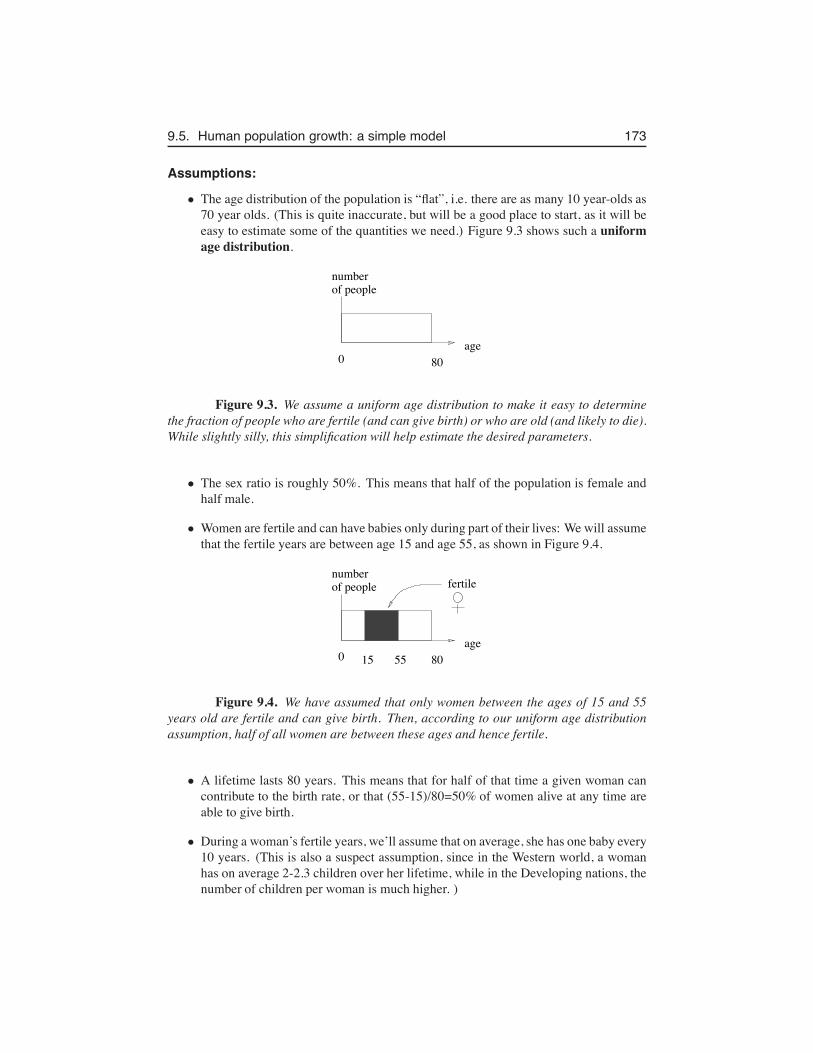
9.5. Human population growth: a simple model 173
Assumptions:
• The age distribution of the population is “flat”, i.e. there are as many 10 year-olds as70 year olds. (This is quite inaccurate, but will be a good place to start, as it will beeasy to estimate some of the quantities we need.) Figure 9.3 shows such a uniformage distribution.
age0 80
number of people
Figure 9.3. We assume a uniform age distribution to make it easy to determinethe fraction of people who are fertile (and can give birth) or who are old (and likely to die).While slightly silly, this simplification will help estimate the desired parameters.
• The sex ratio is roughly 50%. This means that half of the population is female andhalf male.
• Women are fertile and can have babies only during part of their lives: We will assumethat the fertile years are between age 15 and age 55, as shown in Figure 9.4.
age0 80
number of people
15 55
fertile
Figure 9.4. We have assumed that only women between the ages of 15 and 55years old are fertile and can give birth. Then, according to our uniform age distributionassumption, half of all women are between these ages and hence fertile.
• A lifetime lasts 80 years. This means that for half of that time a given woman cancontribute to the birth rate, or that (55-15)/80=50% of women alive at any time areable to give birth.
• During a woman’s fertile years, we’ll assume that on average, she has one baby every10 years. (This is also a suspect assumption, since in the Western world, a womanhas on average 2-2.3 children over her lifetime, while in the Developing nations, thenumber of children per woman is much higher. )
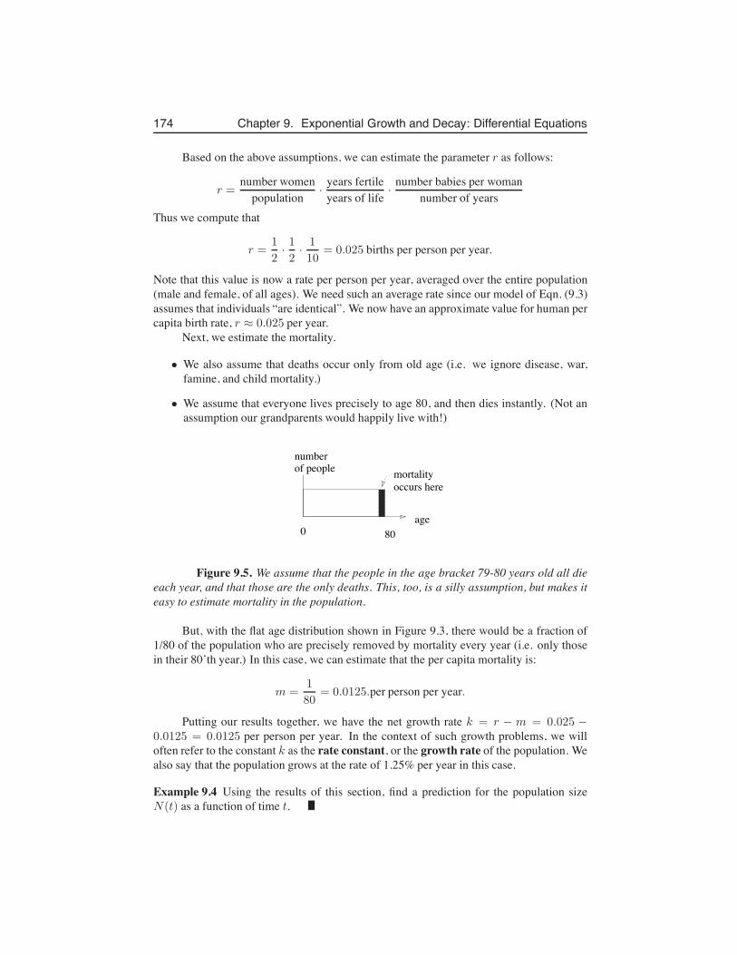
174 Chapter 9. Exponential Growth and Decay: Differential Equations
Based on the above assumptions, we can estimate the parameter r as follows:
r =number women
population·
years fertileyears of life
·number babies per woman
number of yearsThus we compute that
r =1
2·1
2·1
10= 0.025 births per person per year.
Note that this value is now a rate per person per year, averaged over the entire population(male and female, of all ages). We need such an average rate since our model of Eqn. (9.3)assumes that individuals “are identical”. We now have an approximate value for human percapita birth rate, r ≈ 0.025 per year.
Next, we estimate the mortality.
• We also assume that deaths occur only from old age (i.e. we ignore disease, war,famine, and child mortality.)
• We assume that everyone lives precisely to age 80, and then dies instantly. (Not anassumption our grandparents would happily live with!)
age0 80
number of people mortality
occurs here
Figure 9.5. We assume that the people in the age bracket 79-80 years old all dieeach year, and that those are the only deaths. This, too, is a silly assumption, but makes iteasy to estimate mortality in the population.
But, with the flat age distribution shown in Figure 9.3, there would be a fraction of1/80 of the population who are precisely removed by mortality every year (i.e. only thosein their 80’th year.) In this case, we can estimate that the per capita mortality is:
m =1
80= 0.0125.per person per year.
Putting our results together, we have the net growth rate k = r − m = 0.025 −0.0125 = 0.0125 per person per year. In the context of such growth problems, we willoften refer to the constant k as the rate constant, or the growth rate of the population. Wealso say that the population grows at the rate of 1.25% per year in this case.
Example 9.4 Using the results of this section, find a prediction for the population sizeN(t) as a function of time t.
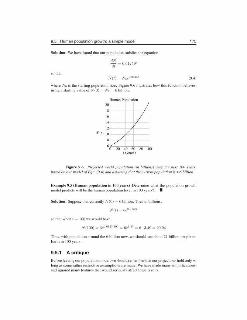
9.5. Human population growth: a simple model 175
Solution: We have found that our population satisfies the equation
dN
dt= 0.0125N
so thatN(t) = N0e
0.0125t (9.4)
where N0 is the starting population size. Figure 9.6 illustrates how this function behaves,using a starting value of N(0) = N0 = 6 billion.
Figure 9.6. Projected world population (in billions) over the next 100 years,based on our model of Eqn. (9.4) and assuming that the current population is ≈6 billion.
Example 9.5 (Human population in 100 years) Determine what the population growthmodel predicts will be the human population level in 100 years?
Solution: Suppose that currently N(0) = 6 billion. Then in billions,
N(t) = 6e0.0125t
so that when t = 100 we would have
N(100) = 6e0.0125·100 = 6e1.25 = 6 · 3.49 = 20.94
Thus, with population around the 6 billion now, we should see about 21 billion people onEarth in 100 years.
9.5.1 A critiqueBefore leaving our population model, we should remember that our projections hold only solong as some rather restrictive assumptions are made. We have made many simplifications,and ignored many features that would seriously affect these results.
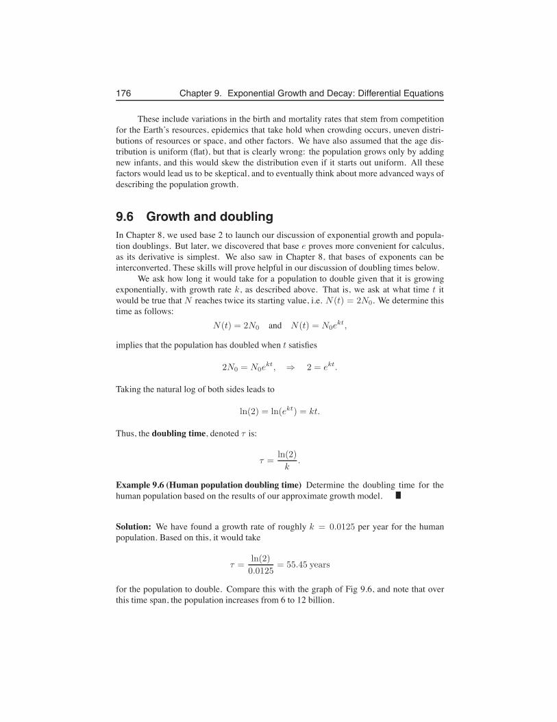
176 Chapter 9. Exponential Growth and Decay: Differential Equations
These include variations in the birth and mortality rates that stem from competitionfor the Earth’s resources, epidemics that take hold when crowding occurs, uneven distri-butions of resources or space, and other factors. We have also assumed that the age dis-tribution is uniform (flat), but that is clearly wrong: the population grows only by addingnew infants, and this would skew the distribution even if it starts out uniform. All thesefactors would lead us to be skeptical, and to eventually think about more advanced ways ofdescribing the population growth.
9.6 Growth and doublingIn Chapter 8, we used base 2 to launch our discussion of exponential growth and popula-tion doublings. But later, we discovered that base e proves more convenient for calculus,as its derivative is simplest. We also saw in Chapter 8, that bases of exponents can beinterconverted. These skills will prove helpful in our discussion of doubling times below.
We ask how long it would take for a population to double given that it is growingexponentially, with growth rate k, as described above. That is, we ask at what time t itwould be true that N reaches twice its starting value, i.e. N(t) = 2N0. We determine thistime as follows:
N(t) = 2N0 and N(t) = N0ekt,
implies that the population has doubled when t satisfies
2N0 = N0ekt, ⇒ 2 = ekt.
Taking the natural log of both sides leads to
ln(2) = ln(ekt) = kt.
Thus, the doubling time, denoted τ is:
τ =ln(2)
k.
Example 9.6 (Human population doubling time) Determine the doubling time for thehuman population based on the results of our approximate growth model.
Solution: We have found a growth rate of roughly k = 0.0125 per year for the humanpopulation. Based on this, it would take
τ =ln(2)
0.0125= 55.45 years
for the population to double. Compare this with the graph of Fig 9.6, and note that overthis time span, the population increases from 6 to 12 billion.
9.7. Exponential decay and radioactivity 177
In general, an equation of the form
dy
dt= ky
that represents an exponential growth will have a doubling time of
τ =ln(2)
k.
t
y
y2y
oo
"
Figure 9.7. Doubling time for exponential growth.
This is shown in Figure 9.7. The interesting thing that we discovered is that thepopulation doubles every 55 years! So that, for example, after 110 years there have beentwo doublings, or a quadrupling of the population.
Example 9.7 (A ten year doubling time) Suppose we are told that some animal popula-tion doubles every 10 years. What growth rate would lead to such a trend?
Solution: Rearranging
t2 =ln(2)
k
we obtaink =
ln(2)
t2=
0.6931
10≈ 0.07 per year.
Thus, we may say that a growth rate of 7% leads to doubling roughly every 10 years.
9.7 Exponential decay and radioactivityA radioactive material consists of atoms that undergo a spontaneous change. Every sooften, an atom will emit a particle, and change to another form. We call this a process ofradioactive decay.
178 Chapter 9. Exponential Growth and Decay: Differential Equations
For any one atom, it is impossible to predict when this event would occur. However,if we have very many atoms, on average some fraction, k, will undergo this decay duringany given unit time. (This fraction will depend on the material.) This means that ky of theamount will be lost per unit time.
We will define y(t) to be the amount of radioactivity remaining at time t. This quan-tity can be measured with Geiger counters, and will depend on time. In the decay process,radioactivity will be continually lost. Thus
[rate of change of y] = −[amount lost per unit time] ⇒dy
dt= −ky.
We see again, a (by now) familiar differential equation.Suppose that initially, there was an amount y0. Then the initial condition that comes
with this differential equation isy(0) = y0.
From familiarity with the differential equation, we know that the function that satisfies itwill be
y(t) = Ce−kt
and using the initial condition will specify that
y(t) = y0e−kt.
For k > 0 a constant, this is a decreasing function of time that we refer to as exponentialdecay.
9.7.1 The half lifeGiven a process of exponential decay, we can ask how long it would take for half of theoriginal amount to remain. That is, we look for t such that
y(t) =y02.
We will refer to the value of t that satisfies this as the half life.
Example 9.8 (Half life) Determine the half life in the exponential decay described above
Solution: We compute:y02
= y0e−kt ⇒
1
2= e−kt.
Now taking reciprocals:2 =
1
e−kt= ekt.
Thus we find the same result as in our calculation for doubling times, namely,
ln(2) = ln(ekt) = kt,
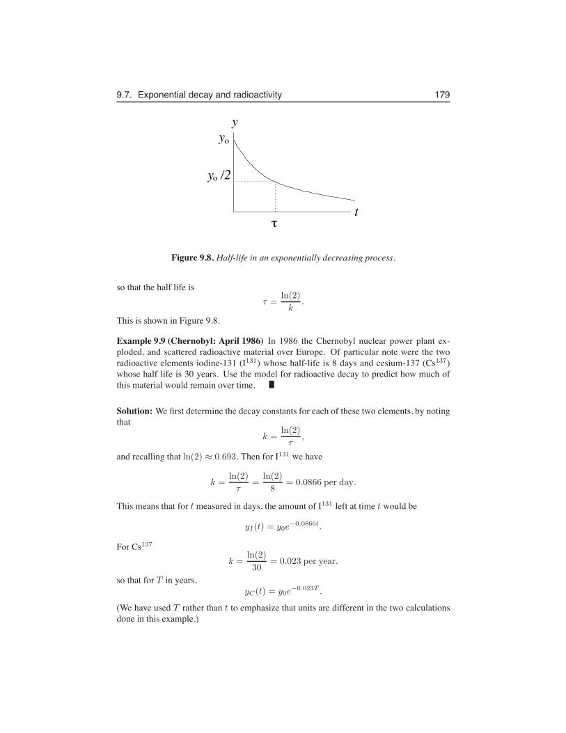
9.7. Exponential decay and radioactivity 179
t
y
τ
y
y /2ο
ο
Figure 9.8. Half-life in an exponentially decreasing process.
so that the half life isτ =
ln(2)
k.
This is shown in Figure 9.8.
Example 9.9 (Chernobyl: April 1986) In 1986 the Chernobyl nuclear power plant ex-ploded, and scattered radioactive material over Europe. Of particular note were the tworadioactive elements iodine-131 (I131) whose half-life is 8 days and cesium-137 (Cs137)whose half life is 30 years. Use the model for radioactive decay to predict how much ofthis material would remain over time.
Solution: We first determine the decay constants for each of these two elements, by notingthat
k =ln(2)
τ,
and recalling that ln(2) ≈ 0.693. Then for I131 we have
k =ln(2)
τ=
ln(2)
8= 0.0866 per day.
This means that for t measured in days, the amount of I131 left at time t would be
yI(t) = y0e−0.0866t.
For Cs137
k =ln(2)
30= 0.023 per year.
so that for T in years,yC(t) = y0e
−0.023T .
(We have used T rather than t to emphasize that units are different in the two calculationsdone in this example.)
180 Chapter 9. Exponential Growth and Decay: Differential Equations
Example 9.10 (Decay to 0.1% of the initial level) How long it would take for I131 to de-cay to 0.1 % of its initial level? (Assume that initial level was just after the explosion atChernobyl.)
Solution: We must calculate the time t such that yI = 0.001y0:
0.001y0 = y0e−0.0866t ⇒ 0.001 = e−0.0866t ⇒ ln(0.001) = −0.0866t.
Therefore,t =
ln(0.001)
−0.0866=
−6.9
−0.0866= 79.7 days.
Thus it would take about 80 days for the level of Iodine-131 to decay to 0.1% of its initiallevel.
9.8 Checking (analytic) solutions to a differentialequation
By analytic solution, we mean a “formula” in the form y = f(x). We have seen a numberof examples of simple differential equations in this chapter, and our main purpose was toshow how these arise in the context of a physical or biological process of growth or decay.Most of these examples led to the differential equation
dy
dt= ky
and therefore, by our observations, to its analytic solution, the exponential function
y = f(t) = Cekt.
However, as we will see, there can be many distinct types of differential equations,and it may not always be clear which function is a solution. Finding the correct solutioncan be quite challenging, even to professional mathematicians. We mention two ideas thatare sometimes helpful.
In some cases, we encounter a new differential equation, and we are given a functionthat is believed to satisfy that equation. We can always check and verify that this claim iscorrect (or find it incorrect) by simple differentiation.
9.8.1 Newtons Law of CoolingNewton’s Law of Cooling states that the rate of change of the temperature of an object T ,is proportional to the difference between the ambient (environment) temperature, E, andthe temperature of the object, T . If the temperature of the environment is constant, andthe objects starts out at temperature T0 initially, then the differential equation and initialcondition describing this process is
dT
dt= k(E − T ), T (0) = T0. (9.5)
9.8. Checking (analytic) solutions to a differential equation 181
The parameter k is a constant that represents the properties of the material. (Some objectsconduct heat better than others, and thus cool off or heat up more quickly. The readershould be able to figure out that these types of objects have higher values of k, as thisimplies larger rates of change per unit time.) We study properties of this equation later, buthere we show how to check which of two possible functions are its solutions.
Example 9.11 (Candidate 1:) Consider the function T (t) = T0e−kt. Show that this sim-ple exponential function is NOT usually a solution to the differential equation (9.5) forNewton’s Law of Cooling.
Solution: We observe, first that this function does satisfy the initial condition, T (0) = T0
by plugging t = 0 into the function:
T (0) = T0e−k·0 = T0.
Next, by simply differentiating the above “candidate function”, we find that its derivativeis
dT
dt= −T0ke
−kt.
To satisfy the differential equation, we must have
dT
dt= k(E − T ). (9.6)
The term on the right hand side would lead to the expression
k(E − T0e−kt)
once the candidate function T (t) is substituted for T . However, in general,
dT
dt= −T0ke
−kt $= k(E − T0e−kt).
(Only in the case that E = 0 do the two sides match, but for arbitrary ambient temperature,this is not the case.) Thus the simple exponential function T (t) = T0e−kt is NOT asolution to this differential equation when E $= 0.
Example 9.12 (Candidate 2:) Show that the modified function
T (t) = E + (T0 − E)e−kt (9.7)
is a solution to the differential equation chap9:eqNLC-diffeqOnly and initial value T (0) =T0.
Solution: Note, first, that by plugging the initial time, t = 0, into the function in Eqn. (9.7)we have
T (0) = E + (T0 − E)e−k·0 = E + (T0 − E) · 1 = E + (T0 − E) = T0.
182 Chapter 9. Exponential Growth and Decay: Differential Equations
Thus the initial condition is satisfied by the given function.Second, we must show that the derivative dT/dt of the function in (9.7) agrees with
the expression k(E − T ) so that the differential equation is satisfied.We compute the derivative of the function in (9.7) and find it to be is
dT
dt=
d
dt
(
E + (T0 − E)e−kt)
= −k(T0 − E)e−kt.
(This follows from the fact that E is a constant, (T0 − E) is constant, and from the chainrule applied to the exponent −kt.) Next, we compute the expression k(E − T ) whereT = T (t) is the function in in (9.7):
k(E − T ) = k(E − [E + (T0 − E)e−kt]) = −k(T0 − E)e−kt.
We now observe agreement between the terms obtained from each of the right and lefthand sides of the differential equation, applied to the above function. We conclude thatthe differential equation is satisfied, so that indeed this candidate function is a solution, asclaimed.
Example 9.13 (Height of water draining out of a cylindrical container:) A cylindrical con-tainer with cross-sectional area A contains water. When a small hole of area a is openedat its base, the water leaks out. It can be shown that height of water h(t) in the containersatisfies the differential equation
dh
dt= −
a
A
√
2gh = −k√h. (9.8)
where k is a constant that depends on the size and shape of the cylinder and its hole:k = a
A
√2g, where g is the acceleration due to gravity. Show that the function
h(t) =
(
√
h0 − kt
2
)2
. (9.9)
is a solution to the differential equation (9.8) and the initial condition h(0) = h0.
Solution: By plugging in t = 0, we see that h(0) = h0 in (9.9). Thus, the initial conditionis satisfied. To show that the differential equation (9.8) is satisfied, we differentiate thefunction in (9.9):
dh(t)
dt=
d
dt
(
√
h0 − kt
2
)2
= 2
(
√
h0 − kt
2
)
·(
−k
2
)
= −k
(
√
h0 − kt
2
)
.
Here we have used the power law and the chain rule, remembering that h0, k are constants.Now we notice that, using (9.9), the expression for
√
h(t) exactly matches what we havecomputed for dh/dt. Thus, we have shown that the function in (9.9) satisfies both the initialcondition and the differential equation. Remark: The derivation of the differential equationfrom physical principles, and the calculation that discovers its solution is discussed in asecond semester calculus course.
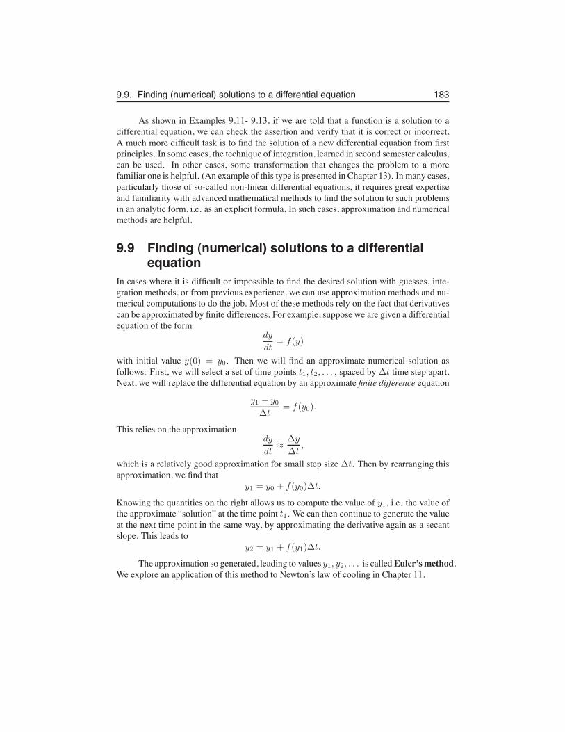
9.9. Finding (numerical) solutions to a differential equation 183
As shown in Examples 9.11- 9.13, if we are told that a function is a solution to adifferential equation, we can check the assertion and verify that it is correct or incorrect.A much more difficult task is to find the solution of a new differential equation from firstprinciples. In some cases, the technique of integration, learned in second semester calculus,can be used. In other cases, some transformation that changes the problem to a morefamiliar one is helpful. (An example of this type is presented in Chapter 13). In many cases,particularly those of so-called non-linear differential equations, it requires great expertiseand familiarity with advanced mathematical methods to find the solution to such problemsin an analytic form, i.e. as an explicit formula. In such cases, approximation and numericalmethods are helpful.
9.9 Finding (numerical) solutions to a differentialequation
In cases where it is difficult or impossible to find the desired solution with guesses, inte-gration methods, or from previous experience, we can use approximation methods and nu-merical computations to do the job. Most of these methods rely on the fact that derivativescan be approximated by finite differences. For example, suppose we are given a differentialequation of the form
dy
dt= f(y)
with initial value y(0) = y0. Then we will find an approximate numerical solution asfollows: First, we will select a set of time points t1, t2, . . . , spaced by ∆t time step apart.Next, we will replace the differential equation by an approximate finite difference equation
y1 − y0∆t
= f(y0).
This relies on the approximationdy
dt≈
∆y
∆t,
which is a relatively good approximation for small step size ∆t. Then by rearranging thisapproximation, we find that
y1 = y0 + f(y0)∆t.
Knowing the quantities on the right allows us to compute the value of y1, i.e. the value ofthe approximate “solution” at the time point t1. We can then continue to generate the valueat the next time point in the same way, by approximating the derivative again as a secantslope. This leads to
y2 = y1 + f(y1)∆t.
The approximation so generated, leading to values y1, y2, . . . is calledEuler’s method.We explore an application of this method to Newton’s law of cooling in Chapter 11.
184 Chapter 9. Exponential Growth and Decay: Differential Equations
Exercises9.1. A differential equation is an equation in which some function is related to its own
derivative(s). For each of the following functions, calculate the appropriate deriva-tive, and show that the function satisfies the indicated differential equation
(a) f(x) = 2e−3x, f ′(x) = −3f(x)
(b) f(t) = Cekt, f ′(t) = kf(t)
(c) f(t) = 1− e−t, f ′(t) = 1− f(t)
9.2. Consider the function y = f(t) = Cekt where C and k are constants. For whatvalue(s) of these constants does this function satisfy the equation
(a) dydt = −5y,
(b) dydt = 3y.
[Remark: an equation which involves a function and its derivative is called a differ-ential equation.]
9.3. Find a function that satisfies each of the following differential equations. [Remark:all your answers will be exponential functions, but they may have different depen-dent and independent variables.]
(a) dy
dt= −y,
(b) dc
dx= −0.1c and c(0) = 20,
(c) dz
dt= 3z and z(0) = 5.
9.4. If 70% of a radioactive substance remains after one year, find its half-life.9.5. Carbon 14: Carbon 14 has a half-life of 5730 years. This means that after 5730
years, a sample of Carbon 14, which is a radioactive isotope of carbon will have lostone half of its original radioactivity.
(a) Estimate how long it takes for the sample to fall to roughly 0.001 of its originallevel of radioactivity.
(b) Each gram of 14C has an activity given here in units of 12 decays per minute.After some time, the amount of radioactivity decreases. For example, a sample5730 years old has only one half the original activity level, i.e. 6 decays perminute. If a 1 gm sample of material is found to have 45 decays per hour,approximately how old is it? (Note: 14C is used in radiocarbon dating, aprocess by which the age of materials containing carbon can be estimated.W. Libby received the Nobel prize in chemistry in 1960 for developing thistechnique.)
9.6. Strontium-90: Strontium-90 is a radioactive isotope with a half-life of 29 years.If you begin with a sample of 800 units, how long will it take for the amount ofradioactivity of the strontium sample to be reduced to
Exercises 185
(a) 400 units(b) 200 units(c) 1 unit
9.7. More radioactivity: The half-life of a radioactive material is 1620 years.(a) What percentage of the radioactivity will remain after 500 years?(b) Cobalt 60 is a radioactive substance with half life 5.3 years. It is used in
medical application (radiology). How long does it take for 80% of a sample ofthis substance to decay?
9.8. Assume the atmospheric pressure y at a height x meters above the sea level satisfiesthe relation dy
dx= kx. If one day at a certain location the atmospheric pressures
are 760 and 675 torr (unit for pressure) at sea level and at 1000 meters above sealevel, respectively, find the value of the atmospheric pressure at 600 meters abovesea level.
9.9. Population growth and doubling: A population of animals has a per-capita birthrate of b = 0.08 per year and a per-capita death rate of m = 0.01 per year. Thepopulation density, P (t) is found to satisfy the differential equation
dP (t)
dt= bP (t)−mP (t)
(a) If the population is initially P (0) = 1000, find how big the population will bein 5 years.
(b) When will the population double?9.10. Rodent population: The per capita birthrate of one species of rodent is 0.05 new-
borns per day. (This means that, on average, each member of the population willresult in 5 newborn rodents every 100 days.) Suppose that over the period of 1000days there are no deaths, and that the initial population of rodents is 250. Write adifferential equation for the population size N(t) at time t (in days). Write down theinitial condition that N satisfies. Find the solution, i.e. express N as some functionof time t that satisfies your differential equation and initial condition. How manyrodents will there be after 1 year ?
9.11. Growth and extinction of microorganisms:(a) The population y(t) of a certain microorganism grows continuously and fol-
lows an exponential behaviour over time. Its doubling time is found to be0.27 hours. What differential equation would you use to describe its growth? (Note: you will have to find the value of the rate constant, k, using thedoubling time.)
(b) With exposure to ultra-violet radiation, the population ceases to grow, and themicroorganisms continuously die off. It is found that the half-life is then 0.1hours. What differential equation would now describe the population?
9.12. A bacterial population: A bacterial population grows at a rate proportional to thepopulation size at time t. Let y(t) be the population size at time t. By experiment it
186 Chapter 9. Exponential Growth and Decay: Differential Equations
is determined that the population at t = 10 min is 15, 000 and at t = 30 min it is20, 000.
(a) What was the initial population?(b) What will the population be at time t = 60min?
9.13. Antibiotic treatment: A colony of bacteria is treated with a mild antibiotic agent sothat the bacteria start to die. It is observed that the density of bacteria as a function oftime follows the approximate relationship b(t) = 85e−0.5t where t is time in hours.Determine the time it takes for half of the bacteria to disappear (This is called thehalf life.) Find how long it takes for 99% of the bacteria to die.
9.14. Chemical breakdown: In a chemical reaction, a substance S is broken down. Theconcentration of the substance is observed to change at a rate proportional to the cur-rent concentration. It was observed that 1 Mole/liter of S decreased to 0.5 Moles/literin 10 minutes. How long will it take until only 0.25 Moles per liter remain? Untilonly 1% of the original concentration remains?
9.15. Two populations: Two populations are studied. Population 1 is found to obey thedifferential equation
dy1/dt = 0.2y1
and population 2 obeysdy2/dt = −0.3y2
where t is time in years.(a) Which population is growing and which is declining?(b) Find the doubling time (respectively half-life) associated with the given popu-
lation.(c) If the initial levels of the two populations were y1(0) = 100 and y2(0) =
10, 000, how big would each population be at time t ?(d) At what time would the two populations be exactly equal?
9.16. The human population: The human population on Earth doubles roughly every 50years. In October 2000 there were 6.1 billion humans on earth. Determine what thehuman population would be 500 years later under the uncontrolled growth scenario.How many people would have to inhabit each square kilometer of the planet for thispopulation to fit on earth? (Take the circumference of the earth to be 40,000 km forthe purpose of computing its surface area.)
9.17. First order chemical kinetics: When chemists say that a chemical reaction follows“first order kinetics”, they mean that the concentration of the reactant at time t, i.e.c(t), satisfies an equation of the form dc
dt = −rc where r is a rate constant, hereassumed to be positive. Suppose the reaction mixture initially has concentration 1M(“1 molar”) and that after 1 hour there is half this amount.
(a) Find the “half life” of the reactant.(b) Find the value of the rate constant r.(c) Determine how much will be left after 2 hours.(d) When will only 10% of the initial amount be left?
Exercises 187
9.18. Fish in two lakes: Two lakes have populations of fish, but the conditions are quitedifferent in these lakes. In the first lake, the fish population is growing and satisfiesthe differential equation
dy
dt= 0.2y
where t is time in years. At time t = 0 there were 500 fish in this lake. In the secondlake, the population is dying due to pollution. Its population satisfies the differentialequation
dy
dt= −0.1y,
and initially there were 4000 fish in this lake. At what time will the fish populationsin the two lakes be identical?
9.19. A barrel initially contains 2 kg of salt dissolved in 20 L of water. If water flows inthe rate of 0.4 L per minute and the well-mixed salt water solution flows out at thesame rate. How much salt is present after 8 minutes?
9.20. A savings account: You deposit a sum P (“the Principal”) in a savings accountwith an annual interest rate, r and make no withdrawals over the first year. If theinterest is compounded annually, after one year the amount in this account will be
A(1) = P + rP = P (1 + r).
If the interest is compounded semi-annually (once every 1/2 year), then every 6months half of the interest is added to your account, i.e.
A
(
1
2
)
= P +r
2P = P
(
1 +r
2
)
A(1) = A
(
1
2
)
(
1 +r
2
)
= P(
1 +r
2
)(
1 +r
2
)
= P(
1 +r
2
)2
(a) Suppose that you invest $500 in an account with interest rate 4% compoundedsemi-annually. How much money would you have after 6 months? After 1year ? After 10 years ? Roughly how long does it take to double your moneyin this way? How would it differ if the interest was 8% ?
(b) Interest can also be compounded more frequently, for example monthly (i.e.12 times per year, each time with an increment of r/12). Answer the questionsposed in part (a) in this case
(c) Is it better to save your money in a bank with 4% interest compounded monthly,or 5% interest compounded annually?

188 Chapter 9. Exponential Growth and Decay: Differential Equations
Chapter 10
Trigonometric functions
In this chapter we will explore periodic and oscillatory phenomena. The trigonometricfunctions will be the basis for much of what we construct, and hence, we first introducethese and familiarize ourselves with their properties.
10.1 Introduction: angles and circlesAngles can be measured in a number of ways. One way is to assign a value in degrees, withthe convention that one complete revolution is represented by 360◦. Why 360? And what isa degree exactly? Is this some universal measure that any intelligent being (say on Mars orelsewhere) would find appealing? Actually, 360 is a rather arbitrary convention that arosehistorically, and has no particular meaning. We could as easily have had mathematicalancestors that decided to divide circles into 1000 “equal pieces” or 240 or some othersubdivision. It turns out that this measure is not particularly convenient, and we will replaceit by a more universal quantity.
The universal quantity stems from the fact that circles of all sizes have one commongeometric feature: they have the same ratio of circumference to diameter, no matter whattheir size (or where in the universe they occur). We call that ratio π, that is
π =Circumference of circle
Diameter of circle
The diameter D of a circle of radius r is just twice the radius,
D = 2r,
so this naturally leads to the familiar relationship of circumference, C, to radius
C = 2πr.
(But we should not forget that this is merely a definition of the constant π. The moreinteresting conclusion that develops from this definition is that the area of the circle isA = πr2, but we shall see the reason for this later, in the context of areas and integration.)
189
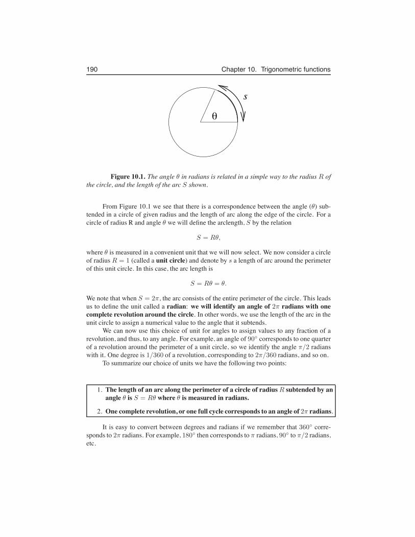
190 Chapter 10. Trigonometric functions
#
s
Figure 10.1. The angle θ in radians is related in a simple way to the radius R ofthe circle, and the length of the arc S shown.
From Figure 10.1 we see that there is a correspondence between the angle (θ) sub-tended in a circle of given radius and the length of arc along the edge of the circle. For acircle of radius R and angle θ we will define the arclength, S by the relation
S = Rθ,
where θ is measured in a convenient unit that we will now select. We now consider a circleof radius R = 1 (called a unit circle) and denote by s a length of arc around the perimeterof this unit circle. In this case, the arc length is
S = Rθ = θ.
We note that when S = 2π, the arc consists of the entire perimeter of the circle. This leadsus to define the unit called a radian: we will identify an angle of 2π radians with onecomplete revolution around the circle. In other words, we use the length of the arc in theunit circle to assign a numerical value to the angle that it subtends.
We can now use this choice of unit for angles to assign values to any fraction of arevolution, and thus, to any angle. For example, an angle of 90◦ corresponds to one quarterof a revolution around the perimeter of a unit circle, so we identify the angle π/2 radianswith it. One degree is 1/360 of a revolution, corresponding to 2π/360 radians, and so on.
To summarize our choice of units we have the following two points:
1. The length of an arc along the perimeter of a circle of radiusR subtended by anangle θ is S = Rθ where θ is measured in radians.
2. One complete revolution, or one full cycle corresponds to an angle of 2π radians.
It is easy to convert between degrees and radians if we remember that 360◦ corre-sponds to 2π radians. For example, 180◦ then corresponds to π radians, 90◦ to π/2 radians,etc.
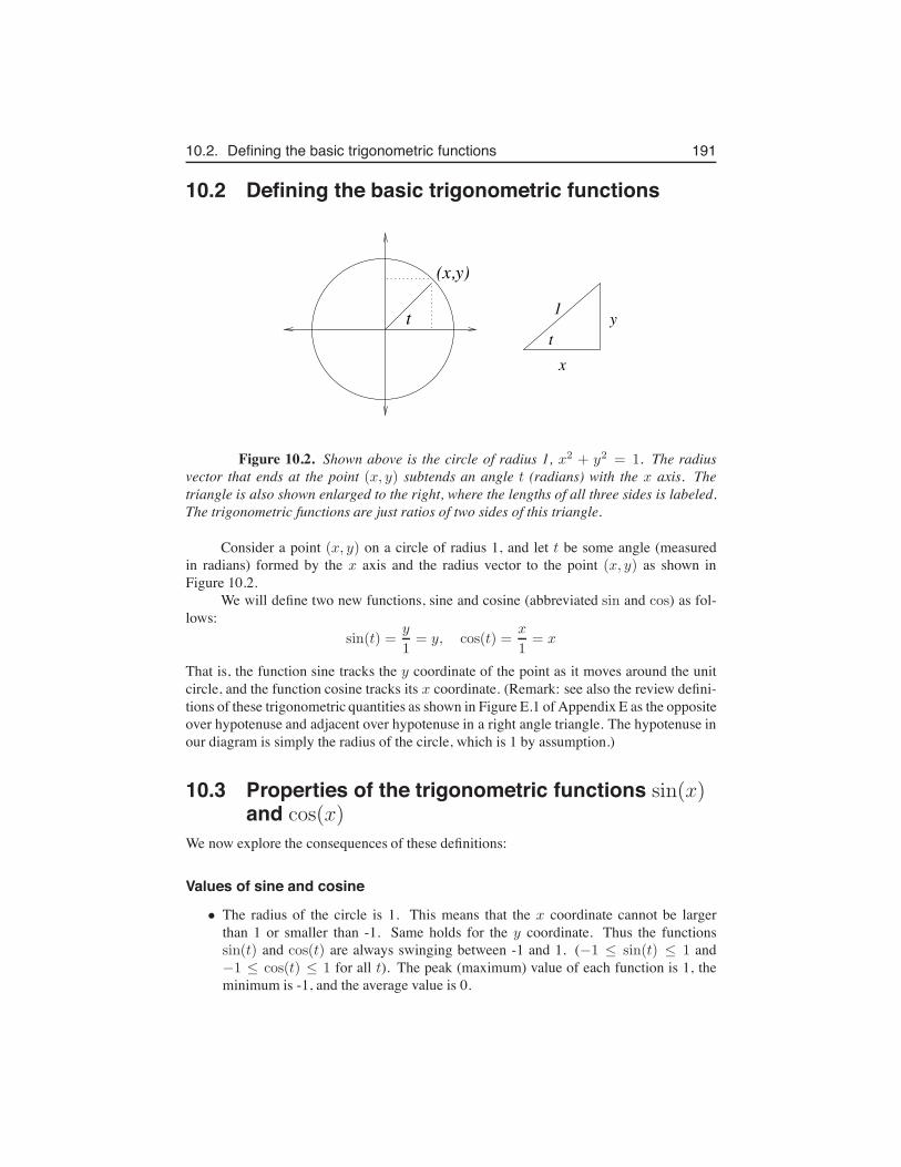
10.2. Defining the basic trigonometric functions 191
10.2 Defining the basic trigonometric functions
tt
y
x
(x,y)
1
Figure 10.2. Shown above is the circle of radius 1, x2 + y2 = 1. The radiusvector that ends at the point (x, y) subtends an angle t (radians) with the x axis. Thetriangle is also shown enlarged to the right, where the lengths of all three sides is labeled.The trigonometric functions are just ratios of two sides of this triangle.
Consider a point (x, y) on a circle of radius 1, and let t be some angle (measuredin radians) formed by the x axis and the radius vector to the point (x, y) as shown inFigure 10.2.
We will define two new functions, sine and cosine (abbreviated sin and cos) as fol-lows:
sin(t) =y
1= y, cos(t) =
x
1= x
That is, the function sine tracks the y coordinate of the point as it moves around the unitcircle, and the function cosine tracks its x coordinate. (Remark: see also the review defini-tions of these trigonometric quantities as shown in Figure E.1 of Appendix E as the oppositeover hypotenuse and adjacent over hypotenuse in a right angle triangle. The hypotenuse inour diagram is simply the radius of the circle, which is 1 by assumption.)
10.3 Properties of the trigonometric functions sin(x)and cos(x)
We now explore the consequences of these definitions:
Values of sine and cosine
• The radius of the circle is 1. This means that the x coordinate cannot be largerthan 1 or smaller than -1. Same holds for the y coordinate. Thus the functionssin(t) and cos(t) are always swinging between -1 and 1. (−1 ≤ sin(t) ≤ 1 and−1 ≤ cos(t) ≤ 1 for all t). The peak (maximum) value of each function is 1, theminimum is -1, and the average value is 0.
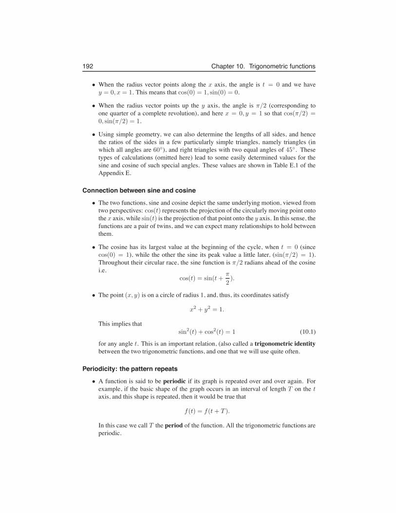
192 Chapter 10. Trigonometric functions
• When the radius vector points along the x axis, the angle is t = 0 and we havey = 0, x = 1. This means that cos(0) = 1, sin(0) = 0.
• When the radius vector points up the y axis, the angle is π/2 (corresponding toone quarter of a complete revolution), and here x = 0, y = 1 so that cos(π/2) =0, sin(π/2) = 1.
• Using simple geometry, we can also determine the lengths of all sides, and hencethe ratios of the sides in a few particularly simple triangles, namely triangles (inwhich all angles are 60◦), and right triangles with two equal angles of 45◦. Thesetypes of calculations (omitted here) lead to some easily determined values for thesine and cosine of such special angles. These values are shown in Table E.1 of theAppendix E.
Connection between sine and cosine
• The two functions, sine and cosine depict the same underlying motion, viewed fromtwo perspectives: cos(t) represents the projection of the circularly moving point ontothe x axis, while sin(t) is the projection of that point onto the y axis. In this sense, thefunctions are a pair of twins, and we can expect many relationships to hold betweenthem.
• The cosine has its largest value at the beginning of the cycle, when t = 0 (sincecos(0) = 1), while the other the sine its peak value a little later, (sin(π/2) = 1).Throughout their circular race, the sine function is π/2 radians ahead of the cosinei.e.
cos(t) = sin(t+π
2).
• The point (x, y) is on a circle of radius 1, and, thus, its coordinates satisfy
x2 + y2 = 1.
This implies thatsin2(t) + cos2(t) = 1 (10.1)
for any angle t. This is an important relation, (also called a trigonometric identitybetween the two trigonometric functions, and one that we will use quite often.
Periodicity: the pattern repeats
• A function is said to be periodic if its graph is repeated over and over again. Forexample, if the basic shape of the graph occurs in an interval of length T on the taxis, and this shape is repeated, then it would be true that
f(t) = f(t+ T ).
In this case we call T the period of the function. All the trigonometric functions areperiodic.
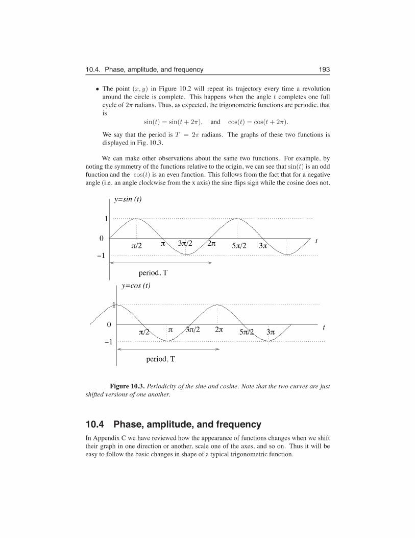
10.4. Phase, amplitude, and frequency 193
• The point (x, y) in Figure 10.2 will repeat its trajectory every time a revolutionaround the circle is complete. This happens when the angle t completes one fullcycle of 2π radians. Thus, as expected, the trigonometric functions are periodic, thatis
sin(t) = sin(t+ 2π), and cos(t) = cos(t+ 2π).
We say that the period is T = 2π radians. The graphs of these two functions isdisplayed in Fig. 10.3.
We can make other observations about the same two functions. For example, bynoting the symmetry of the functions relative to the origin, we can see that sin(t) is an oddfunction and the cos(t) is an even function. This follows from the fact that for a negativeangle (i.e. an angle clockwise from the x axis) the sine flips sign while the cosine does not.
3!2!!!/2 3!/2 5!/2
1
$1
0
y=sin (t)
t
period, T
3!2!!!/2 3!/2 5!/2
1
$1
0 t
period, T
y=cos (t)
Figure 10.3. Periodicity of the sine and cosine. Note that the two curves are justshifted versions of one another.
10.4 Phase, amplitude, and frequencyIn Appendix C we have reviewed how the appearance of functions changes when we shifttheir graph in one direction or another, scale one of the axes, and so on. Thus it will beeasy to follow the basic changes in shape of a typical trigonometric function.
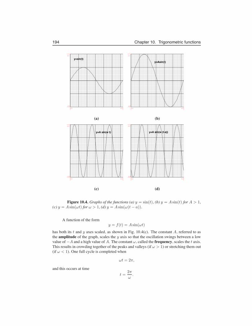
194 Chapter 10. Trigonometric functions
y=sin(t)
0.0 6.3-2.0
2.0
y=Asin(t)
0.0 6.3-2.0
2.0
(a) (b)
y=A sin(w t)
0.0 6.3-2.0
2.0
y=A sin(w (t-a))
0.0 6.3-2.0
2.0
(c) (d)
Figure 10.4. Graphs of the functions (a) y = sin(t), (b) y = A sin(t) for A > 1,(c) y = A sin(ωt) for ω > 1, (d) y = A sin(ω(t− a)).
A function of the formy = f(t) = A sin(ωt)
has both its t and y axes scaled, as shown in Fig. 10.4(c). The constant A, referred to asthe amplitude of the graph, scales the y axis so that the oscillation swings between a lowvalue of −A and a high value of A. The constant ω, called the frequency, scales the t axis.This results in crowding together of the peaks and valleys (if ω > 1) or stretching them out(if ω < 1). One full cycle is completed when
ωt = 2π,
and this occurs at timet =
2π
ω.
10.5. Rhythmic processes 195
We will use the symbol T , to denote this special time, and we refer to T as the period. Wenote the connection between frequency and period:
ω =2π
T, ⇒ T =
2π
ω.
If we examine a graph of function
y = f(t) = A sin(ω(t− a))
we find that the graph has been shifted in the positive t direction by a, as in Fig. 10.4(d).We note that at time t = a, the value of the function is
y = f(t) = A sin(ω(a− a)) = A sin(0) = 0.
This tells us that the cycle “starts” with a delay, i.e. the value of y goes through zero whenwhen t = a.
Another common variant of the same function can be written in the form
y = f(t) = A sin(ωt− φ).
Here φ is called the phase shift of the oscillation. Comparing the above two related forms,we see that they are the same if we identify φ with ωa. The phase shift, φ is consideredto be a quantity without units, whereas the quantity a has units of time, same as t. Whenφ = 2π, (which is the same as the case that a = 2π/ω, the graph has been moved over tothe right by one full period. (Naturally, when the graph is so moved, it looks the same as itdid originally, since each cycle is the same as the one before, and same as the one after.)
Some of the scaled, shifted, sine functions described here are shown in Figure 10.4.
10.5 Rhythmic processesMany natural phenomena are cyclic. It is often convenient to represent such phenomenawith one or another simple periodic functions, and sine and cosine can be adapted forthe purpose. The idea is to pick the right function, the right frequency (or period), theamplitude, and possibly the phase shift, so as to represent the desired behaviour.
To select one or another of these functions, it helps to remember that cosine starts acycle (at t = 0) at its peak value, while sine starts the cycle at 0, i.e., at its average value. Afunction that starts at the lowest point of the cycle is − cos(t). In most cases, the choice offunction to use is somewhat arbitrary, since a phase shift can correct for the phase at whichthe oscillation starts.
Next, we pick a constant ω such that the trigonometric function sin(ωt) (or cos(ωt))has the correct period. Given a period for the oscillation, T , recall that the correspondingfrequency is simply ω = 2π
T . We then select the amplitude, and horizontal and verticalshifts to complete the mission. The examples below illustrate this process.
Example 10.1 (Daylight hours:) In Vancouver, the shortest day (8 hours of light) occursaround December 22, and the longest day (16 hours of light) is around June 21. Approxi-mate the cyclic changes of daylight through the season using the sine function.
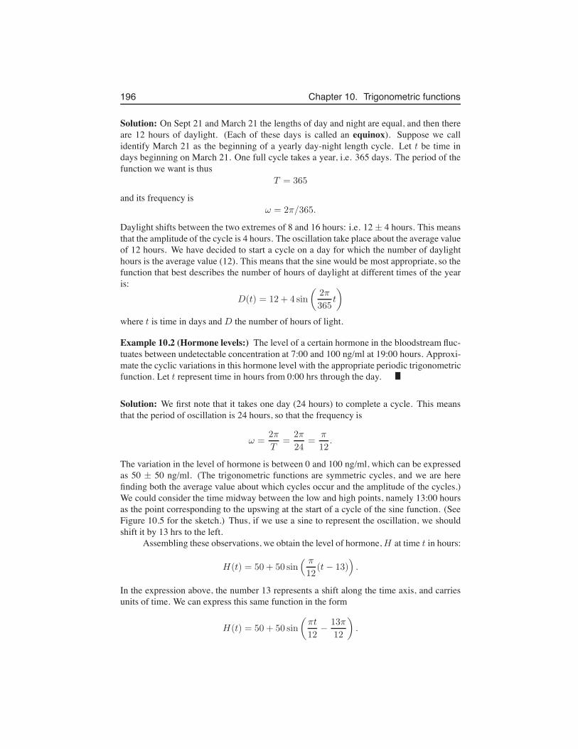
196 Chapter 10. Trigonometric functions
Solution: On Sept 21 and March 21 the lengths of day and night are equal, and then thereare 12 hours of daylight. (Each of these days is called an equinox). Suppose we callidentify March 21 as the beginning of a yearly day-night length cycle. Let t be time indays beginning on March 21. One full cycle takes a year, i.e. 365 days. The period of thefunction we want is thus
T = 365
and its frequency isω = 2π/365.
Daylight shifts between the two extremes of 8 and 16 hours: i.e. 12 ± 4 hours. This meansthat the amplitude of the cycle is 4 hours. The oscillation take place about the average valueof 12 hours. We have decided to start a cycle on a day for which the number of daylighthours is the average value (12). This means that the sine would be most appropriate, so thefunction that best describes the number of hours of daylight at different times of the yearis:
D(t) = 12 + 4 sin
(
2π
365t
)
where t is time in days and D the number of hours of light.
Example 10.2 (Hormone levels:) The level of a certain hormone in the bloodstream fluc-tuates between undetectable concentration at 7:00 and 100 ng/ml at 19:00 hours. Approxi-mate the cyclic variations in this hormone level with the appropriate periodic trigonometricfunction. Let t represent time in hours from 0:00 hrs through the day.
Solution: We first note that it takes one day (24 hours) to complete a cycle. This meansthat the period of oscillation is 24 hours, so that the frequency is
ω =2π
T=
2π
24=
π
12.
The variation in the level of hormone is between 0 and 100 ng/ml, which can be expressedas 50 ± 50 ng/ml. (The trigonometric functions are symmetric cycles, and we are herefinding both the average value about which cycles occur and the amplitude of the cycles.)We could consider the time midway between the low and high points, namely 13:00 hoursas the point corresponding to the upswing at the start of a cycle of the sine function. (SeeFigure 10.5 for the sketch.) Thus, if we use a sine to represent the oscillation, we shouldshift it by 13 hrs to the left.
Assembling these observations, we obtain the level of hormone, H at time t in hours:
H(t) = 50 + 50 sin( π
12(t− 13)
)
.
In the expression above, the number 13 represents a shift along the time axis, and carriesunits of time. We can express this same function in the form
H(t) = 50 + 50 sin
(
πt
12−
13π
12
)
.
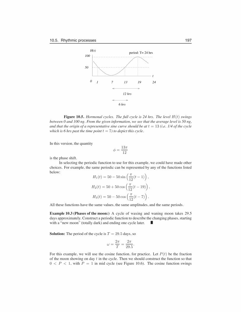
10.5. Rhythmic processes 197
0 7 191 13
50
100
t
12 hrs
6 hrs
H(t)
24
period: T= 24 hrs
Figure 10.5. Hormonal cycles. The full cycle is 24 hrs. The level H(t) swingsbetween 0 and 100 ng. From the given information, we see that the average level is 50 ng,and that the origin of a representative sine curve should be at t = 13 (i.e. 1/4 of the cyclewhich is 6 hrs past the time point t = 7) to depict this cycle.
In this version, the quantityφ =
13π
12
is the phase shift.In selecting the periodic function to use for this example, we could have made other
choices. For example, the same periodic can be represented by any of the functions listedbelow:
H1(t) = 50− 50 sin( π
12(t− 1)
)
,
H2(t) = 50 + 50 cos( π
12(t− 19)
)
,
H3(t) = 50− 50 cos( π
12(t− 7)
)
.
All these functions have the same values, the same amplitudes, and the same periods.
Example 10.3 (Phases of the moon:) A cycle of waxing and waning moon takes 29.5days approximately. Construct a periodic function to describe the changing phases, startingwith a “new moon” (totally dark) and ending one cycle later.
Solution: The period of the cycle is T = 29.5 days, so
ω =2π
T=
2π
29.5.
For this example, we will use the cosine function, for practice. Let P (t) be the fractionof the moon showing on day t in the cycle. Then we should construct the function so that0 < P < 1, with P = 1 in mid cycle (see Figure 10.6). The cosine function swings
198 Chapter 10. Trigonometric functions
0 29.5
Figure 10.6. Periodic moon phases
between the values -1 and 1. To obtain a positive function in the desired range for P (t), wewill add a constant and scale the cosine as follows:
1
2[1 + cos(ωt)].
This is not quite right, though because at t = 0 this function takes the value 1, rather than0, as shown in Figure 10.6. To correct this we can either introduce a phase shift, i.e. set
P (t) =1
2[1 + cos(ωt+ π)].
(Then when t = 0, we get P (t) = 0.5[1 + cosπ] = 0.5[1− 1] = 0.) or we can write
P (t) =1
2[1− cos(ωt+ π)],
which achieves the same result.
10.6 Other trigonometric functionsAlthough we shall mostly be concerned with the two basic functions described above,several others are historically important and are encountered frequently in integral cal-culus. These include the following: tan(t) = sin(t)/ cos(t), cot(t) = 1/ tan(t), sec(t) =1/ cos(t), and csc(t) = 1 sin(t). We review these and the identities that they satisfy in Ap-pendix E. We also include the Law of Cosines (E.1), and angle-sum identities in the sameappendix.
10.7 Limits involving the trigonometric functionsIn Chapter 3, we zoomed in on the graph of the sine function close to the origin (Fig. 3.2).By doing so, we reasoned that
sin(x) ≈ x, for small x.
Restated, with h replacing the variable x, we would have sin(h) ≈ h for small h, or inmore formal limit notation,
limh→0
sin(h)
h= 1. (10.2)
10.7. Limits involving the trigonometric functions 199
(See (3.1).) This is a very important limit, that will be used directly in computing thederivative of the trigonometric functions using the definition of the derivative.
A similar analysis of the graph of the cosine function, (here omitted) leads to a secondimportant limit:
limh→0
cos(h)− 1
h= 0. (10.3)
We can now apply these to computing derivatives.
10.7.1 Derivatives of the trigonometric functionsLet y = f(x) = sin(x) be the function to differentiate, where x is now the independentvariable (previously called t). Below, we use the definition of the derivative to compute thederivative of this function.
Example 10.4 (Derivative of sin(x):) Compute the derivative of y = sin(x) using thedefinition of the derivative.
Solution: We apply the definition of the derivative as follows:
f ′(x) = limh→0
f(x+ h)− f(x)
hd sin(x)
dx= lim
h→0
sin(x+ h)− sin(x)
h
= limh→0
sin(x) cos(h) + sin(h) cos(x) − sin(x)
h
= limh→0
(
sin(x)cos(h)− 1
h+ cos(x)
sin(h)
h
)
= sin(x)
(
limh→0
cos(h)− 1
h
)
+ cos(x)
(
limh→0
sin(h)
h
)
= cos(x).
Observe that the limits (10.2) and (10.3) were used in arriving at our final result.A similar calculation using the function cos(x) leads to the result
d cos(x)
dx= − sin(x).
(The same two limits appear in this calculation as well.) We can now calculate the deriva-tive of the any of the other trigonometric functions using the quotient rule.
Example 10.5 (Derivative of the function tan(x):) Compute the derivative of y = tan(x).
Solution: We apply the quotient rule:
d tan(x)
dx=
[sin(x)]′ cos(x) − [cos(x)]′ sin(x)
cos2(x)
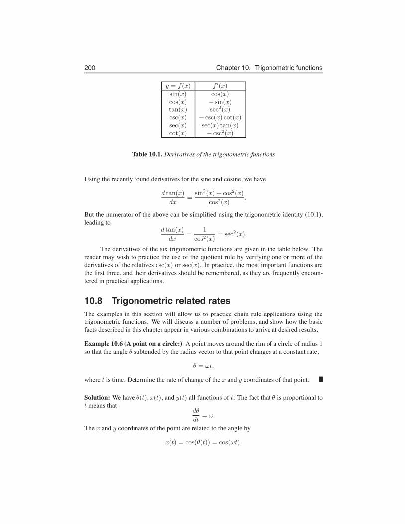
200 Chapter 10. Trigonometric functions
y = f(x) f ′(x)sin(x) cos(x)cos(x) − sin(x)tan(x) sec2(x)csc(x) − csc(x) cot(x)sec(x) sec(x) tan(x)cot(x) − csc2(x)
Table 10.1. Derivatives of the trigonometric functions
Using the recently found derivatives for the sine and cosine, we have
d tan(x)
dx=
sin2(x) + cos2(x)
cos2(x).
But the numerator of the above can be simplified using the trigonometric identity (10.1),leading to
d tan(x)
dx=
1
cos2(x)= sec2(x).
The derivatives of the six trigonometric functions are given in the table below. Thereader may wish to practice the use of the quotient rule by verifying one or more of thederivatives of the relatives csc(x) or sec(x). In practice, the most important functions arethe first three, and their derivatives should be remembered, as they are frequently encoun-tered in practical applications.
10.8 Trigonometric related ratesThe examples in this section will allow us to practice chain rule applications using thetrigonometric functions. We will discuss a number of problems, and show how the basicfacts described in this chapter appear in various combinations to arrive at desired results.
Example 10.6 (A point on a circle:) A point moves around the rim of a circle of radius 1so that the angle θ subtended by the radius vector to that point changes at a constant rate,
θ = ωt,
where t is time. Determine the rate of change of the x and y coordinates of that point.
Solution: We have θ(t), x(t), and y(t) all functions of t. The fact that θ is proportional tot means that
dθ
dt= ω.
The x and y coordinates of the point are related to the angle by
x(t) = cos(θ(t)) = cos(ωt),
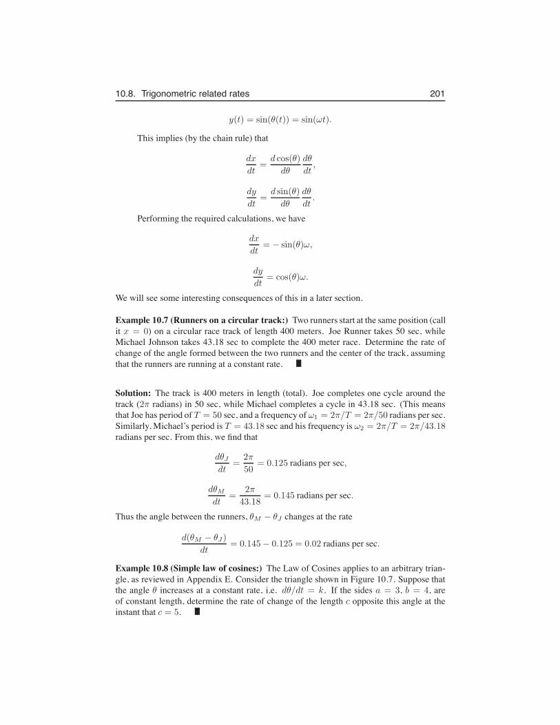
10.8. Trigonometric related rates 201
y(t) = sin(θ(t)) = sin(ωt).
This implies (by the chain rule) that
dx
dt=
d cos(θ)
dθ
dθ
dt,
dy
dt=
d sin(θ)
dθ
dθ
dt.
Performing the required calculations, we have
dx
dt= − sin(θ)ω,
dy
dt= cos(θ)ω.
We will see some interesting consequences of this in a later section.
Example 10.7 (Runners on a circular track:) Two runners start at the same position (callit x = 0) on a circular race track of length 400 meters. Joe Runner takes 50 sec, whileMichael Johnson takes 43.18 sec to complete the 400 meter race. Determine the rate ofchange of the angle formed between the two runners and the center of the track, assumingthat the runners are running at a constant rate.
Solution: The track is 400 meters in length (total). Joe completes one cycle around thetrack (2π radians) in 50 sec, while Michael completes a cycle in 43.18 sec. (This meansthat Joe has period of T = 50 sec, and a frequency of ω1 = 2π/T = 2π/50 radians per sec.Similarly, Michael’s period is T = 43.18 sec and his frequency is ω2 = 2π/T = 2π/43.18radians per sec. From this, we find that
dθJdt
=2π
50= 0.125 radians per sec,
dθMdt
=2π
43.18= 0.145 radians per sec.
Thus the angle between the runners, θM − θJ changes at the rate
d(θM − θJ)
dt= 0.145− 0.125 = 0.02 radians per sec.
Example 10.8 (Simple law of cosines:) The Law of Cosines applies to an arbitrary trian-gle, as reviewed in Appendix E. Consider the triangle shown in Figure 10.7. Suppose thatthe angle θ increases at a constant rate, i.e. dθ/dt = k. If the sides a = 3, b = 4, areof constant length, determine the rate of change of the length c opposite this angle at theinstant that c = 5.
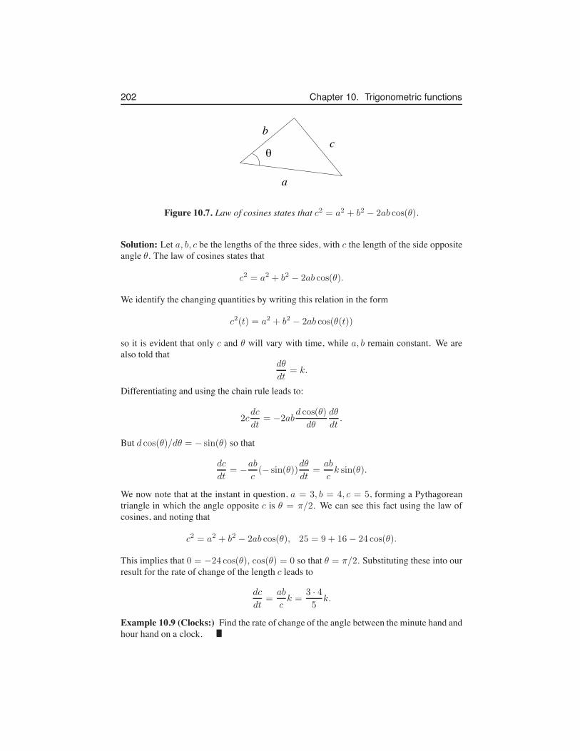
202 Chapter 10. Trigonometric functions
a
bc
θ
Figure 10.7. Law of cosines states that c2 = a2 + b2 − 2ab cos(θ).
Solution: Let a, b, c be the lengths of the three sides, with c the length of the side oppositeangle θ. The law of cosines states that
c2 = a2 + b2 − 2ab cos(θ).
We identify the changing quantities by writing this relation in the form
c2(t) = a2 + b2 − 2ab cos(θ(t))
so it is evident that only c and θ will vary with time, while a, b remain constant. We arealso told that
dθ
dt= k.
Differentiating and using the chain rule leads to:
2cdc
dt= −2ab
d cos(θ)
dθ
dθ
dt.
But d cos(θ)/dθ = − sin(θ) so that
dc
dt= −
ab
c(− sin(θ))
dθ
dt=
ab
ck sin(θ).
We now note that at the instant in question, a = 3, b = 4, c = 5, forming a Pythagoreantriangle in which the angle opposite c is θ = π/2. We can see this fact using the law ofcosines, and noting that
c2 = a2 + b2 − 2ab cos(θ), 25 = 9 + 16− 24 cos(θ).
This implies that 0 = −24 cos(θ), cos(θ) = 0 so that θ = π/2. Substituting these into ourresult for the rate of change of the length c leads to
dc
dt=
ab
ck =
3 · 45
k.
Example 10.9 (Clocks:) Find the rate of change of the angle between the minute hand andhour hand on a clock.
10.8. Trigonometric related rates 203
x
#1
2 #x
#1$#2
(a) (b)
Figure 10.8. Figure for Examples 10.9 and 10.10.
Solution: We will call θ1 the angle that the minute hand subtends with the x axis (horizon-tal direction) and θ2 the angle that the hour hand makes with the same axis.
If our clock is working properly, each hand will move around at a constant rate.The hour hand will trace out one complete revolution (2π radians) every 12 hours, whilethe minute hand will complete a revolution every hour. Both hands move in a clockwisedirection, which (by convention) is towards negative angles. This means that
dθ1dt
= −2π radians per hour,
dθ2dt
= −2π
12radians per hour.
The angle between the two hands is the difference of the two angles, i.e.
θ = θ1 − θ2.
Thus,dθ
dt=
d
dt(θ1 − θ2) =
dθ1dt
−dθ2dt
= −2π +2π
12.
We find that the rate of change of the angle between the hands is
dθ
dt= −2π
11
12= −π
11
6.
Example 10.10 (Clocks, continued:) Suppose that the length of the minute hand is 4 cmand the length of the hour hand is 3 cm. At what rate is the distance between the handschanging when it is 3:00 o’clock?
Solution: We use the law of cosines to give us the rate of change of the desired distance.We have the triangle shown in figure 10.8 in which side lengths are a = 3, b = 4, and c(t)opposite the angle θ(t). From the previous example, we have
dc
dt=
ab
csin(θ)
dθ
dt.
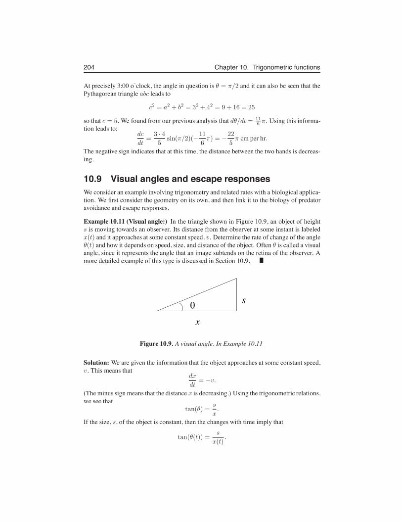
204 Chapter 10. Trigonometric functions
At precisely 3:00 o’clock, the angle in question is θ = π/2 and it can also be seen that thePythagorean triangle abc leads to
c2 = a2 + b2 = 32 + 42 = 9 + 16 = 25
so that c = 5. We found from our previous analysis that dθ/dt = 116 π. Using this informa-
tion leads to:dc
dt=
3 · 45
sin(π/2)(−11
6π) = −
22
5π cm per hr.
The negative sign indicates that at this time, the distance between the two hands is decreas-ing.
10.9 Visual angles and escape responsesWe consider an example involving trigonometry and related rates with a biological applica-tion. We first consider the geometry on its own, and then link it to the biology of predatoravoidance and escape responses.
Example 10.11 (Visual angle:) In the triangle shown in Figure 10.9, an object of heights is moving towards an observer. Its distance from the observer at some instant is labeledx(t) and it approaches at some constant speed, v. Determine the rate of change of the angleθ(t) and how it depends on speed, size, and distance of the object. Often θ is called a visualangle, since it represents the angle that an image subtends on the retina of the observer. Amore detailed example of this type is discussed in Section 10.9.
x
sθ
Figure 10.9. A visual angle. In Example 10.11
Solution: We are given the information that the object approaches at some constant speed,v. This means that
dx
dt= −v.
(The minus sign means that the distance x is decreasing.) Using the trigonometric relations,we see that
tan(θ) =s
x.
If the size, s, of the object is constant, then the changes with time imply that
tan(θ(t)) =s
x(t).
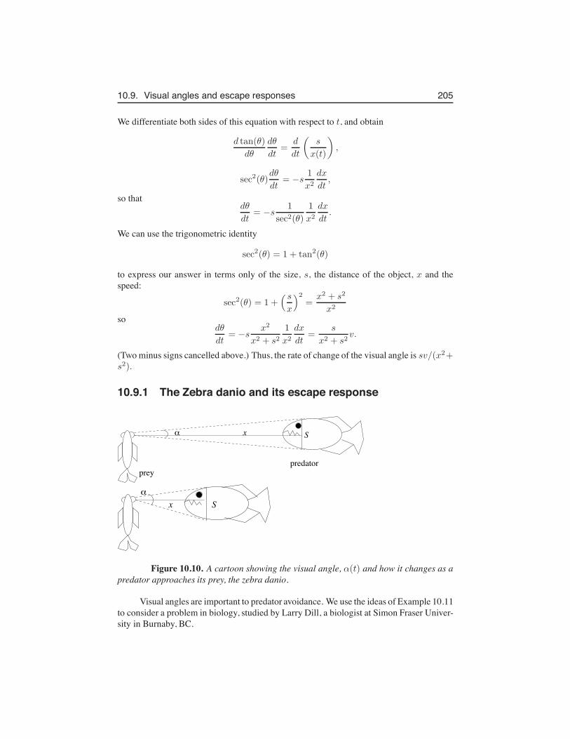
10.9. Visual angles and escape responses 205
We differentiate both sides of this equation with respect to t, and obtain
d tan(θ)
dθ
dθ
dt=
d
dt
(
s
x(t)
)
,
sec2(θ)dθ
dt= −s
1
x2
dx
dt,
so thatdθ
dt= −s
1
sec2(θ)
1
x2
dx
dt.
We can use the trigonometric identity
sec2(θ) = 1 + tan2(θ)
to express our answer in terms only of the size, s, the distance of the object, x and thespeed:
sec2(θ) = 1 +( s
x
)2=
x2 + s2
x2
sodθ
dt= −s
x2
x2 + s21
x2
dx
dt=
s
x2 + s2v.
(Two minus signs cancelled above.) Thus, the rate of change of the visual angle is sv/(x2+s2).
10.9.1 The Zebra danio and its escape response
% x S
preypredator
S%
x
Figure 10.10. A cartoon showing the visual angle, α(t) and how it changes as apredator approaches its prey, the zebra danio.
Visual angles are important to predator avoidance. We use the ideas of Example 10.11to consider a problem in biology, studied by Larry Dill, a biologist at Simon Fraser Univer-sity in Burnaby, BC.
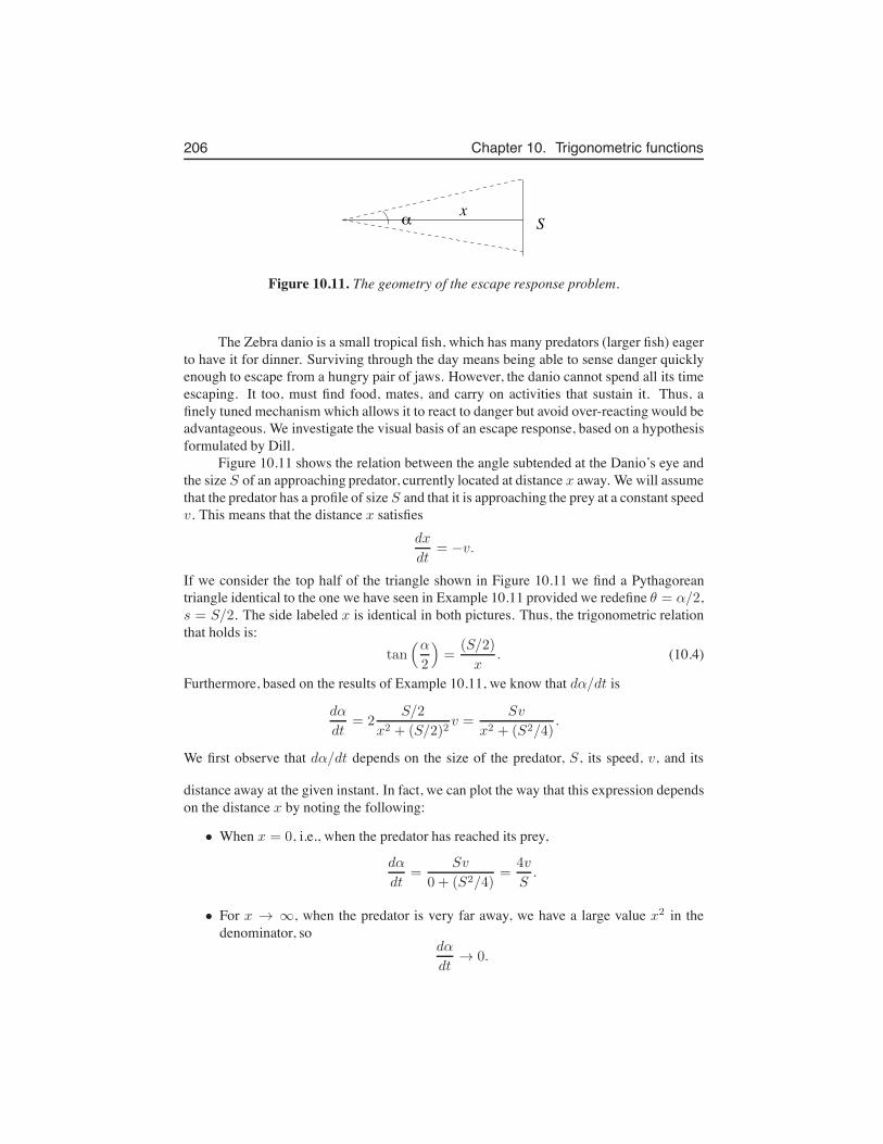
206 Chapter 10. Trigonometric functions
% xS
Figure 10.11. The geometry of the escape response problem.
The Zebra danio is a small tropical fish, which has many predators (larger fish) eagerto have it for dinner. Surviving through the day means being able to sense danger quicklyenough to escape from a hungry pair of jaws. However, the danio cannot spend all its timeescaping. It too, must find food, mates, and carry on activities that sustain it. Thus, afinely tuned mechanism which allows it to react to danger but avoid over-reacting would beadvantageous. We investigate the visual basis of an escape response, based on a hypothesisformulated by Dill.
Figure 10.11 shows the relation between the angle subtended at the Danio’s eye andthe size S of an approaching predator, currently located at distance x away. We will assumethat the predator has a profile of size S and that it is approaching the prey at a constant speedv. This means that the distance x satisfies
dx
dt= −v.
If we consider the top half of the triangle shown in Figure 10.11 we find a Pythagoreantriangle identical to the one we have seen in Example 10.11 provided we redefine θ = α/2,s = S/2. The side labeled x is identical in both pictures. Thus, the trigonometric relationthat holds is:
tan(α
2
)
=(S/2)
x. (10.4)
Furthermore, based on the results of Example 10.11, we know that dα/dt is
dα
dt= 2
S/2
x2 + (S/2)2v =
Sv
x2 + (S2/4).
We first observe that dα/dt depends on the size of the predator, S, its speed, v, and its
distance away at the given instant. In fact, we can plot the way that this expression dependson the distance x by noting the following:
• When x = 0, i.e., when the predator has reached its prey,
dα
dt=
Sv
0 + (S2/4)=
4v
S.
• For x → ∞, when the predator is very far away, we have a large value x2 in thedenominator, so
dα
dt→ 0.
10.9. Visual angles and escape responses 207
A rough sketch of the way that the rate of change of the visual angle depends on thecurrent distance to the predator is shown in the curve on Figure 10.12.
10.9.2 When to escape?What sort of visual input should the danio respond to, if it is to be efficient at avoiding thepredator? In principle, we would like to consider a response that has the following features
• If the predator is too far away, if it is moving slowly, or if it is moving in the oppositedirection, it should appear harmless and should not cause undue panic and inappro-priate escape response, since this uses up the prey’s energy to no good purpose.
• If the predator is coming quickly towards the danio, and approaching directly, itshould be perceived as a threat and should trigger the escape response.
In keeping with these reasonable expectations, the hypothesis proposed by Dill isthat:
The escape response is triggered when the predator approaches so quickly, thatthe rate of change of the visual angle is greater than some critical value.
We will call that critical value Kcrit. This constant would depend on how “skittish”the Danio is given factors such as perceived risks of its environment. This means that theescape response is triggered in the Danio when
dα
dt= Kcrit
i.e. whenKcrit =
Sv
x2 + (S2/4).
Figure 10.12(a) illustrates geometrically a solution to this equation. We show the liney = Kcrit and the curve y = Sv/(x2 + (S2/4)) superimposed on the same coordinatesystem. The value of x, labeled xreact will be the distance of the predator at the instant thatthe Danio realizes that it is under threat and should escape. We can determine the value ofthis distance, referred to as the reaction distance, by solving for x.
10.9.3 Large slow predators beat Danio’s escape responseFigure 10.12(b) illustrates a possibility where there is no distance at which which Kcrit =Sv/(x2 + (S2/4)). This may happen if either the Danio has a very high threshold of alert,so that it fails to react to threats, or if the curve depicting dα/dt is too low. That happenseither if S is very large (big predator) or if v is small (slow moving predator “sneaking up”on its prey). From this scenario, we find that in some situations, the fate of the Danio wouldbe sealed in the jaws of its pursuer.
To determine how far away the predator is detected in the happier scenario of Fig-ure 10.12(a), we solve for the reaction distance, xreact:
x2 + (S2/4) =Sv
Kcrit⇒ xreact =
√
Sv
Kcrit−
S2
4=
√
S
(
v
Kcrit−
S
4
)
.
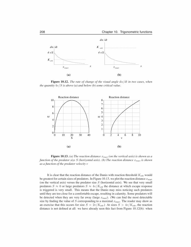
208 Chapter 10. Trigonometric functions
x
4 v/S
critK
% d /dt
x reactx
4 v/S
x react
d /dt %
K crit
(a) (b)
Figure 10.12. The rate of change of the visual angle dα/dt in two cases, whenthe quantity 4v/S is above (a) and below (b) some critical value.
(a) (b)
Figure 10.13. (a) The reaction distance xreact (on the vertical axis) is shown as afunction of the predator size S (horizontal axis). (b) The reaction distance xreact is shownas a function of the predator velocity v
It is clear that the reaction distance of the Danio with reaction threshold Kcrit wouldbe greatest for certain sizes of predators. In Figure 10.13, we plot the reaction distance xreact(on the vertical axis) versus the predator size S (horizontal axis). We see that very smallpredators S ≈ 0 or large predators S ≈ 4v/Kcrit the distance at which escape responseis triggered is very small. This means that the Danio may miss noticing such predatorsuntil they are too close for a comfortable escape, resulting in calamity. Some predators willbe detected when they are very far away (large xreact). (We can find the most detectablesize by finding the value of S corresponding to a maximal xreact. The reader may show asan exercise that this occurs for size S = 2v/Kcrit.) At sizes S > 4v/Kcrit, the reactiondistance is not defined at all: we have already seen this fact from Figure 10.12(b): when
10.9. Visual angles and escape responses 209
Kcrit > 4v/S, the straight line and the curve fail to intersect, and there is no solution.Figure 10.13(b) illustrates the dependence of the reaction distance xreact on the speed
v of the predator. We find that for small values of v, i.e. v < KcritS/4, xreact is not defined:the Danio would not notice the threat posed by predators that swim very slowly.
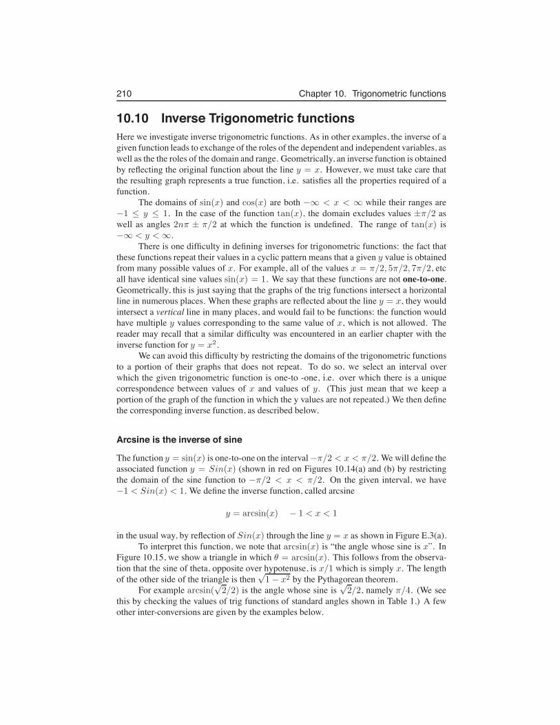
210 Chapter 10. Trigonometric functions
10.10 Inverse Trigonometric functionsHere we investigate inverse trigonometric functions. As in other examples, the inverse of agiven function leads to exchange of the roles of the dependent and independent variables, aswell as the the roles of the domain and range. Geometrically, an inverse function is obtainedby reflecting the original function about the line y = x. However, we must take care thatthe resulting graph represents a true function, i.e. satisfies all the properties required of afunction.
The domains of sin(x) and cos(x) are both −∞ < x < ∞ while their ranges are−1 ≤ y ≤ 1. In the case of the function tan(x), the domain excludes values ±π/2 aswell as angles 2nπ ± π/2 at which the function is undefined. The range of tan(x) is−∞ < y < ∞.
There is one difficulty in defining inverses for trigonometric functions: the fact thatthese functions repeat their values in a cyclic pattern means that a given y value is obtainedfrom many possible values of x. For example, all of the values x = π/2, 5π/2, 7π/2, etcall have identical sine values sin(x) = 1. We say that these functions are not one-to-one.Geometrically, this is just saying that the graphs of the trig functions intersect a horizontalline in numerous places. When these graphs are reflected about the line y = x, they wouldintersect a vertical line in many places, and would fail to be functions: the function wouldhave multiple y values corresponding to the same value of x, which is not allowed. Thereader may recall that a similar difficulty was encountered in an earlier chapter with theinverse function for y = x2.
We can avoid this difficulty by restricting the domains of the trigonometric functionsto a portion of their graphs that does not repeat. To do so, we select an interval overwhich the given trigonometric function is one-to -one, i.e. over which there is a uniquecorrespondence between values of x and values of y. (This just mean that we keep aportion of the graph of the function in which the y values are not repeated.) We then definethe corresponding inverse function, as described below.
Arcsine is the inverse of sine
The function y = sin(x) is one-to-one on the interval −π/2 < x < π/2. We will define theassociated function y = Sin(x) (shown in red on Figures 10.14(a) and (b) by restrictingthe domain of the sine function to −π/2 < x < π/2. On the given interval, we have−1 < Sin(x) < 1. We define the inverse function, called arcsine
y = arcsin(x) − 1 < x < 1
in the usual way, by reflection of Sin(x) through the line y = x as shown in Figure E.3(a).To interpret this function, we note that arcsin(x) is “the angle whose sine is x”. In
Figure 10.15, we show a triangle in which θ = arcsin(x). This follows from the observa-tion that the sine of theta, opposite over hypotenuse, is x/1 which is simply x. The lengthof the other side of the triangle is then
√1− x2 by the Pythagorean theorem.
For example arcsin(√2/2) is the angle whose sine is
√2/2, namely π/4. (We see
this by checking the values of trig functions of standard angles shown in Table 1.) A fewother inter-conversions are given by the examples below.
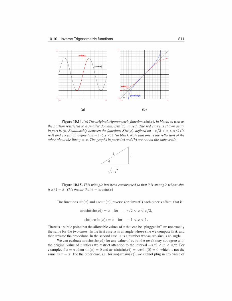
10.10. Inverse Trigonometric functions 211
y=sin(x)
y=Sin(x)
-6.3 6.3-1.5
1.5
y=x
y=Sin(x)
y=arcsin(x)
-1.5 1.5-1.5
1.5
(a) (b)
Figure 10.14. (a) The original trigonometric function, sin(x), in black, as well asthe portion restricted to a smaller domain, Sin(x), in red. The red curve is shown againin part b. (b) Relationship between the functions Sin(x), defined on −π/2 < x < π/2 (inred) and arcsin(x) defined on −1 < x < 1 (in blue). Note that one is the reflection of theother about the line y = x. The graphs in parts (a) and (b) are not on the same scale.
#
1
1!x2
x
Figure 10.15. This triangle has been constructed so that θ is an angle whose sineis x/1 = x. This means that θ = arcsin(x)
The functions sin(x) and arcsin(x), reverse (or “invert”) each other’s effect, that is:
arcsin(sin(x)) = x for − π/2 < x < π/2,
sin(arcsin(x)) = x for − 1 < x < 1.
There is a subtle point that the allowable values of x that can be “plugged in” are not exactlythe same for the two cases. In the first case, x is an angle whose sine we compute first, andthen reverse the procedure. In the second case, x is a number whose arc-sine is an angle.
We can evaluate arcsin(sin(x)) for any value of x, but the result may not agree withthe original value of x unless we restrict attention to the interval −π/2 < x < π/2. Forexample, if x = π, then sin(x) = 0 and arcsin(sin(x)) = arcsin(0) = 0, which is not thesame as x = π. For the other case, i.e. for sin(arcsin(x)), we cannot plug in any value of
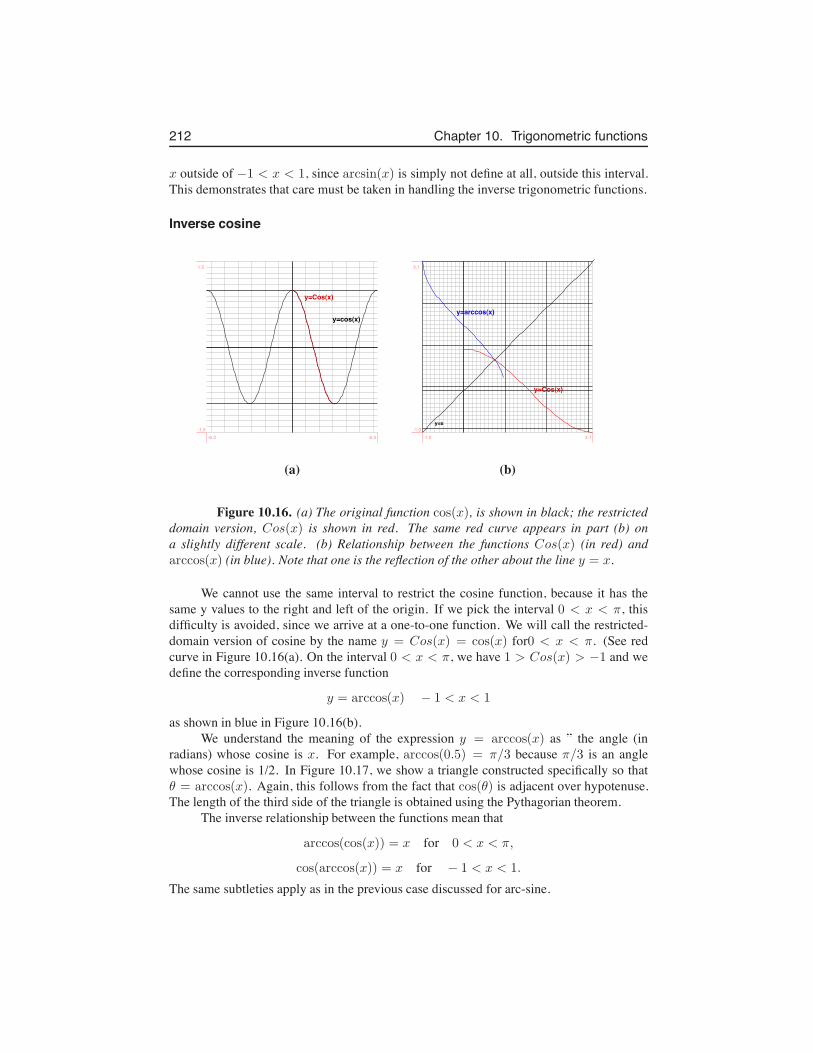
212 Chapter 10. Trigonometric functions
x outside of −1 < x < 1, since arcsin(x) is simply not define at all, outside this interval.This demonstrates that care must be taken in handling the inverse trigonometric functions.
Inverse cosine
y=cos(x)
y=Cos(x)
-6.3 6.3-1.5
1.5
y=x
y=Cos(x)
y=arccos(x)
-1.0 3.1-1.0
3.1
(a) (b)
Figure 10.16. (a) The original function cos(x), is shown in black; the restricteddomain version, Cos(x) is shown in red. The same red curve appears in part (b) ona slightly different scale. (b) Relationship between the functions Cos(x) (in red) andarccos(x) (in blue). Note that one is the reflection of the other about the line y = x.
We cannot use the same interval to restrict the cosine function, because it has thesame y values to the right and left of the origin. If we pick the interval 0 < x < π, thisdifficulty is avoided, since we arrive at a one-to-one function. We will call the restricted-domain version of cosine by the name y = Cos(x) = cos(x) for0 < x < π. (See redcurve in Figure 10.16(a). On the interval 0 < x < π, we have 1 > Cos(x) > −1 and wedefine the corresponding inverse function
y = arccos(x) − 1 < x < 1
as shown in blue in Figure 10.16(b).We understand the meaning of the expression y = arccos(x) as ” the angle (in
radians) whose cosine is x. For example, arccos(0.5) = π/3 because π/3 is an anglewhose cosine is 1/2. In Figure 10.17, we show a triangle constructed specifically so thatθ = arccos(x). Again, this follows from the fact that cos(θ) is adjacent over hypotenuse.The length of the third side of the triangle is obtained using the Pythagorian theorem.
The inverse relationship between the functions mean that
arccos(cos(x)) = x for 0 < x < π,
cos(arccos(x)) = x for − 1 < x < 1.
The same subtleties apply as in the previous case discussed for arc-sine.
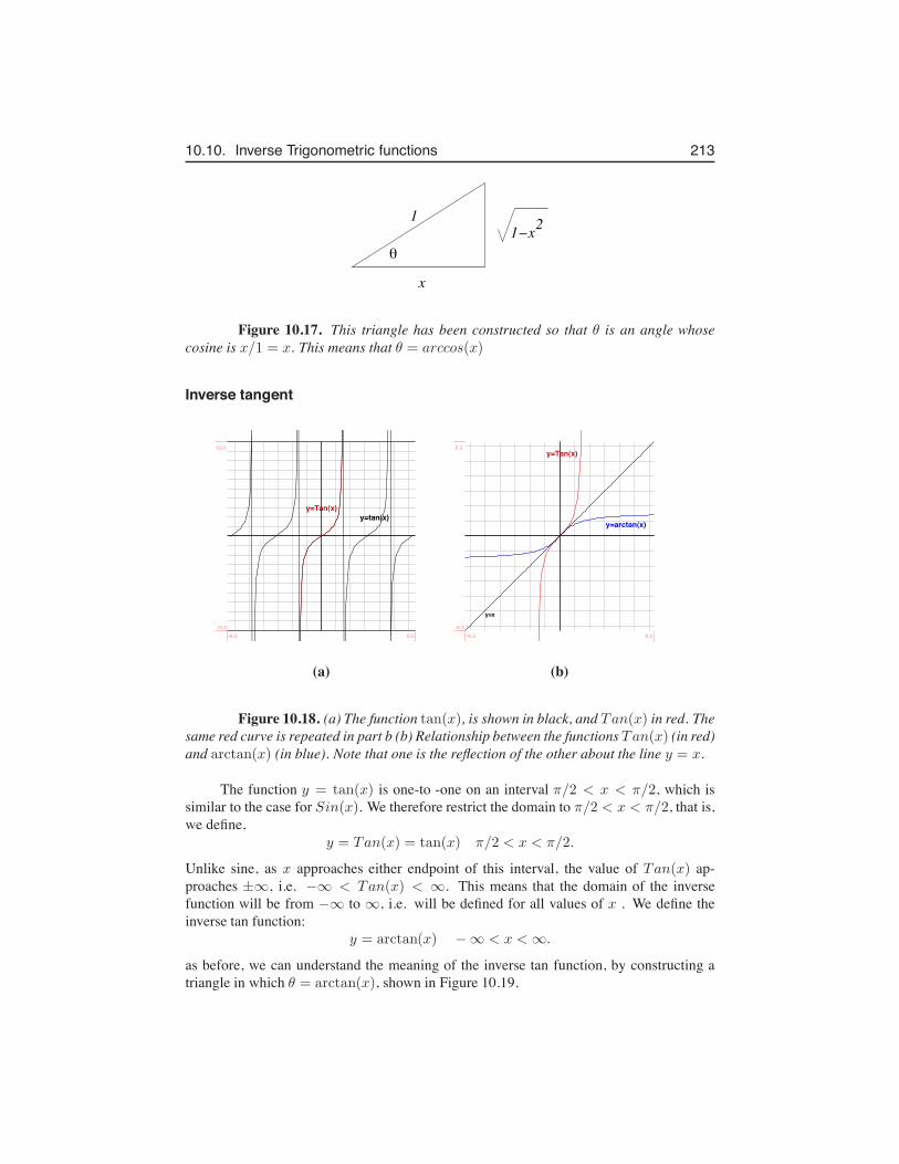
10.10. Inverse Trigonometric functions 213
#
x
11!x2
Figure 10.17. This triangle has been constructed so that θ is an angle whosecosine is x/1 = x. This means that θ = arccos(x)
Inverse tangent
y=tan(x)y=Tan(x)
-6.5 6.5-10.0
10.0
y=x
y=Tan(x)
y=arctan(x)
-6.3 6.3-6.3
6.3
(a) (b)
Figure 10.18. (a) The function tan(x), is shown in black, and Tan(x) in red. Thesame red curve is repeated in part b (b) Relationship between the functions Tan(x) (in red)and arctan(x) (in blue). Note that one is the reflection of the other about the line y = x.
The function y = tan(x) is one-to -one on an interval π/2 < x < π/2, which issimilar to the case for Sin(x). We therefore restrict the domain to π/2 < x < π/2, that is,we define,
y = Tan(x) = tan(x) π/2 < x < π/2.
Unlike sine, as x approaches either endpoint of this interval, the value of Tan(x) ap-proaches ±∞, i.e. −∞ < Tan(x) < ∞. This means that the domain of the inversefunction will be from −∞ to ∞, i.e. will be defined for all values of x . We define theinverse tan function:
y = arctan(x) −∞ < x < ∞.
as before, we can understand the meaning of the inverse tan function, by constructing atriangle in which θ = arctan(x), shown in Figure 10.19.
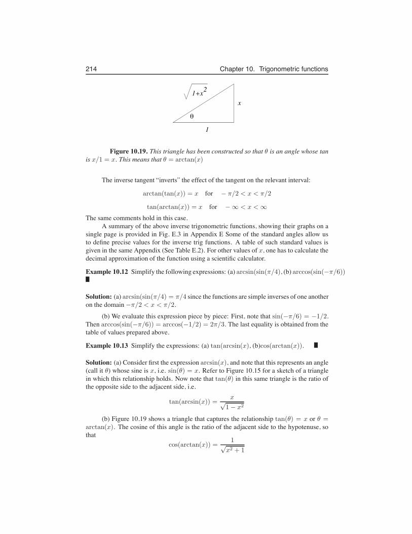
214 Chapter 10. Trigonometric functions
#
x
2
1
1+x
Figure 10.19. This triangle has been constructed so that θ is an angle whose tanis x/1 = x. This means that θ = arctan(x)
The inverse tangent “inverts” the effect of the tangent on the relevant interval:
arctan(tan(x)) = x for − π/2 < x < π/2
tan(arctan(x)) = x for −∞ < x < ∞The same comments hold in this case.
A summary of the above inverse trigonometric functions, showing their graphs on asingle page is provided in Fig. E.3 in Appendix E Some of the standard angles allow usto define precise values for the inverse trig functions. A table of such standard values isgiven in the same Appendix (See Table E.2). For other values of x, one has to calculate thedecimal approximation of the function using a scientific calculator.
Example 10.12 Simplify the following expressions: (a) arcsin(sin(π/4), (b) arccos(sin(−π/6))
Solution: (a) arcsin(sin(π/4) = π/4 since the functions are simple inverses of one anotheron the domain −π/2 < x < π/2.
(b) We evaluate this expression piece by piece: First, note that sin(−π/6) = −1/2.Then arccos(sin(−π/6)) = arccos(−1/2) = 2π/3. The last equality is obtained from thetable of values prepared above.
Example 10.13 Simplify the expressions: (a) tan(arcsin(x), (b)cos(arctan(x)).
Solution: (a) Consider first the expression arcsin(x), and note that this represents an angle(call it θ) whose sine is x, i.e. sin(θ) = x. Refer to Figure 10.15 for a sketch of a trianglein which this relationship holds. Now note that tan(θ) in this same triangle is the ratio ofthe opposite side to the adjacent side, i.e.
tan(arcsin(x)) =x√
1− x2
(b) Figure 10.19 shows a triangle that captures the relationship tan(θ) = x or θ =arctan(x). The cosine of this angle is the ratio of the adjacent side to the hypotenuse, sothat
cos(arctan(x)) =1√
x2 + 1
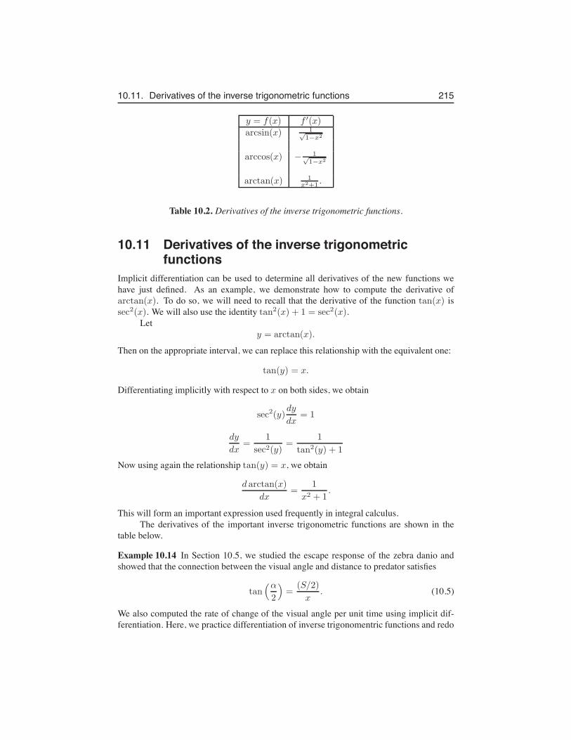
10.11. Derivatives of the inverse trigonometric functions 215
y = f(x) f ′(x)arcsin(x) 1√
1−x2
arccos(x) − 1√1−x2
arctan(x) 1x2+1 .
Table 10.2. Derivatives of the inverse trigonometric functions.
10.11 Derivatives of the inverse trigonometricfunctions
Implicit differentiation can be used to determine all derivatives of the new functions wehave just defined. As an example, we demonstrate how to compute the derivative ofarctan(x). To do so, we will need to recall that the derivative of the function tan(x) issec2(x). We will also use the identity tan2(x) + 1 = sec2(x).
Lety = arctan(x).
Then on the appropriate interval, we can replace this relationship with the equivalent one:
tan(y) = x.
Differentiating implicitly with respect to x on both sides, we obtain
sec2(y)dy
dx= 1
dy
dx=
1
sec2(y)=
1
tan2(y) + 1
Now using again the relationship tan(y) = x, we obtain
d arctan(x)
dx=
1
x2 + 1.
This will form an important expression used frequently in integral calculus.The derivatives of the important inverse trigonometric functions are shown in the
table below.
Example 10.14 In Section 10.5, we studied the escape response of the zebra danio andshowed that the connection between the visual angle and distance to predator satisfies
tan(α
2
)
=(S/2)
x. (10.5)
We also computed the rate of change of the visual angle per unit time using implicit dif-ferentiation. Here, we practice differentiation of inverse trigonomentric functions and redo
216 Chapter 10. Trigonometric functions
the same calculation using these functions. Use the inverse function arctan to restate theangle α in Eqn. 10.5 as a function of x. Then differentiate that function using the chainrule to compute dα/dt.
Solution: We can restate this relationship using the inverse trigonometric function arctanas follows:
α
2= arctan
(
S
2x
)
.
Our experience with the derivative of this function will be useful below. Since both theangle α and the distance from the predator x change with time, we indicate so by writing
α(t) = 2 arctan
(
S
2x(t)
)
.
We apply the chain rule to this expression to calculate the rate of change of the angle αwith respect to time. Let u = S/2x. Recall that S is a constant. Then the derivative of theinverse trigonometric function,
d arctan(u)
du=
1
u2 + 1
and the chain rule leads to
dα(t)
dt=
d arctan(u)
du
du
dx
dx
dt=
1
u2 + 1
(
−S
2x2(t)
)
(−v).
By simplifying, we arrive at the same result, namely that
dα
dt=
Sv
x2 + (S2/4).
This is the rate of change of the visual angle, and agrees with Example 10.11.
10.12 For further study: Trigonometric functions anddifferential equations
As we have seen in this chapter, the functions sin(t) and cos(t) are related to one anothervia differentiation: one is the derivative of the other (with a multiple of the factor (-1).):
d sin(t)
dt= cos(t),
d cos(t)
dt= − sin(t).
The connection becomes even clearer when we examine the second derivatives of thesefunctions:
d2 sin(t)
dt2=
d cos(t)
dt= − sin(t),
d2 cos(t)
dt2= −
d sin(t)
dt= − cos(t).
Thus, for each of the functions y = sin(t), y = cos(t), we find that the function and itssecond derivative are related to one another by the differential equation (DE) d2y/dt2 =
10.13. Additional examples: Implicit differentiation 217
−y. Here the highest derivative is a second derivative, and we denote this as a secondorder DE.
More generally, we make the following observations. These follow by the samereasoning, where the chain rule is applied in differentiation.
The functionsx(t) = cos(ωt), y(t) = sin(ωt)
satisfy a pair of differential equations,
dx
dt= −ωy,
dy
dt= ωx.
The functionsx(t) = cos(ωt), y(t) = sin(ωt)
also satisfy a related differential equation with a second derivative
d2x
dt2= −ω2x.
Students of physics will here recognize the equation that governs the behaviour of aharmonic oscillator, and will see the connection between the circular motion of our pointon the circle, and the differential equation for periodic motion.
10.13 Additional examples: Implicit differentiationThis section is dedicated to practicing implicit differentiation in the context of trigonomet-ric functions.
A surface that looks like an “egg carton” can be described by the function
z = sin(x) cos(y)
See Figure 10.20(a) for the shape of this surface.Suppose we slice though the surface at various levels. We would then see a collection
of circular contours, as found on a topographical map of a mountain range. Such contoursare called level curves, and some of these can be seen in Figure 10.20. We will here beinterested in the contours formed at some specific height, e.g. at height z = 1/2. This setof curves can be described by the equation:
sin(x) cos(y) =1
2.
Let us look at one of these, e.g. the curve shown in Figure 10.20(b). This is justone of the contours, namely the one located in the portion of the graph for −1 < y < 1,0 < x < 3. We practice implicit differentiation for this curve, i.e. we find the slope oftangent lines to this curve.
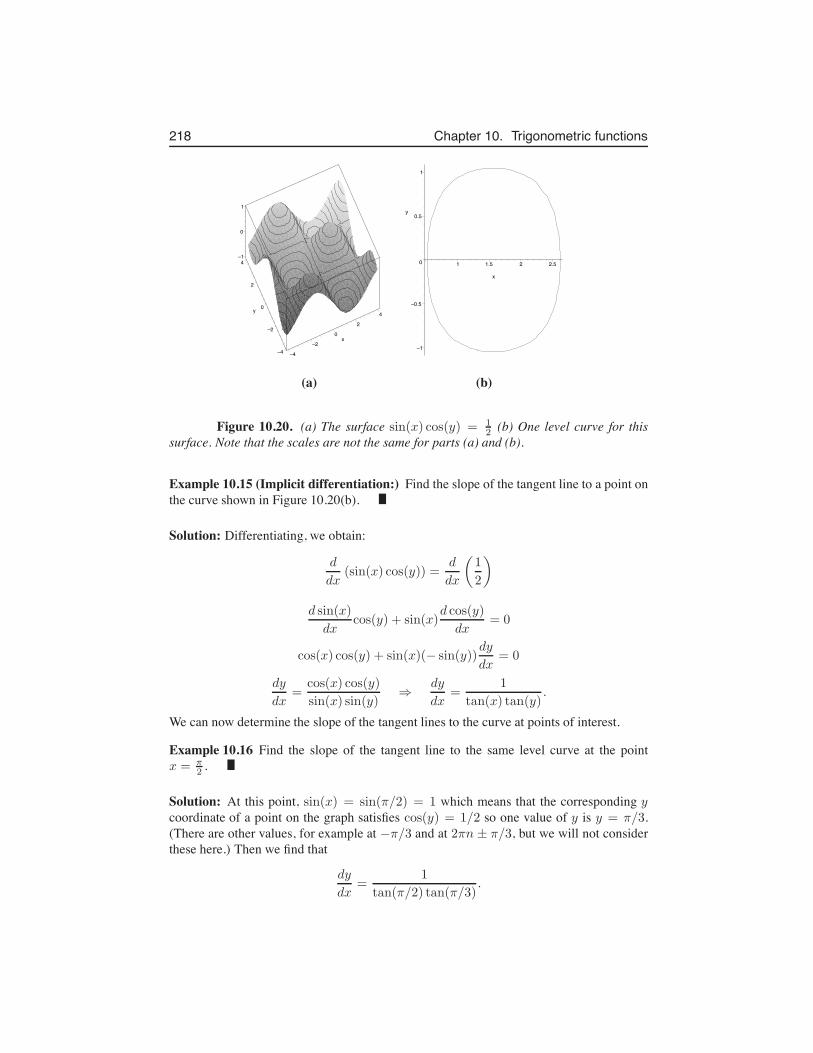
218 Chapter 10. Trigonometric functions
–4
–2
0
2
4
x
–4
–2
0
2
4
y
–1
0
1
–1
–0.5
0
0.5
1
y
1 1.5 2 2.5
x
(a) (b)
Figure 10.20. (a) The surface sin(x) cos(y) = 12 (b) One level curve for this
surface. Note that the scales are not the same for parts (a) and (b).
Example 10.15 (Implicit differentiation:) Find the slope of the tangent line to a point onthe curve shown in Figure 10.20(b).
Solution: Differentiating, we obtain:
d
dx(sin(x) cos(y)) =
d
dx
(
1
2
)
d sin(x)
dxcos(y) + sin(x)
d cos(y)
dx= 0
cos(x) cos(y) + sin(x)(− sin(y))dy
dx= 0
dy
dx=
cos(x) cos(y)
sin(x) sin(y)⇒
dy
dx=
1
tan(x) tan(y).
We can now determine the slope of the tangent lines to the curve at points of interest.
Example 10.16 Find the slope of the tangent line to the same level curve at the pointx = π
2 .
Solution: At this point, sin(x) = sin(π/2) = 1 which means that the corresponding ycoordinate of a point on the graph satisfies cos(y) = 1/2 so one value of y is y = π/3.(There are other values, for example at −π/3 and at 2πn ± π/3, but we will not considerthese here.) Then we find that
dy
dx=
1
tan(π/2) tan(π/3).
10.13. Additional examples: Implicit differentiation 219
But tan(π/2) = ∞ so that the ratio above leads to dydx = 0. The tangent line is horizontal
as it goes though the point (π/2,π/3) on the graph.
Example 10.17 Find the slope of the tangent line to the same level curve at the pointx = π
4 .
Solution: Here we have sin(x) = sin(π/4) =√2/2, and we find that the y coordinate
satisfies √2
2cos(y) =
1
2
This means that cos(y) = 1√2=
√22 so that y = π/4. Thus
dy
dx=
1
tan(π/4) tan(π/4)=
1
1= 1
so that the tangent line at the point (π/4,π/4) has slope 1.
220 Chapter 10. Trigonometric functions
Exercises10.1. Calculate the first derivative for the following functions.
(a) y = sinx2
(b) y = sin2 x
(c) y = cot2 3√x
(d) y = sec(x− 3x2)
(e) y = 2x3 tanx
(f) y = xcosx
(g) y = x cosx
(h) y = e− sin2 1x
(i) y = (2 tan 3x+ 3 cosx)2
(j) y = cos(sinx) + cosx sinx
10.2. Take the derivative of the following functions.(a) f(x) = cos(ln(x4 + 5x2 + 3))
(b) f(x) = sin(√
cos2(x) + x3)
(c) f(x) = 2x3 + log3(x)
(d) f(x) = (x2ex + tan(3x))4
(e) f(x) = x2√
sin3(x) + cos3(x)
10.3. Convert the following expressions in radians to degrees:(a) π (b) 5π/3 (c) 21π/23 (d) 24πConvert the following expressions in degrees to radians:(e) 100o (f) 8o (g) 450o (h) 90oUsing a Pythagorean triangle, evaluate each of the following:(i) cos(π/3) (j) sin(π/4) (k) tan(π/6)
10.4. Graph the following functions over the indicated ranges:(a) y = x sin(x) for −2π < x < 2π
(b) y = ex cos(x) for 0 < x < 4π.10.5. Sketch the graph for each of the following functions:
(a) y =1
2sin 3(x−
π
4)
(b) y = 2− sinx
(c) y = 3 cos 2x
(d) y = 2 cos(1
2x+
π
4)
10.6. The Radian is an important unit associated with angles. One revolution about a circleis equivalent to 360 degrees or 2π radians. Convert the following angles (in degrees)to angles in radians. (Express these as multiples of π, not as decimal expansions):
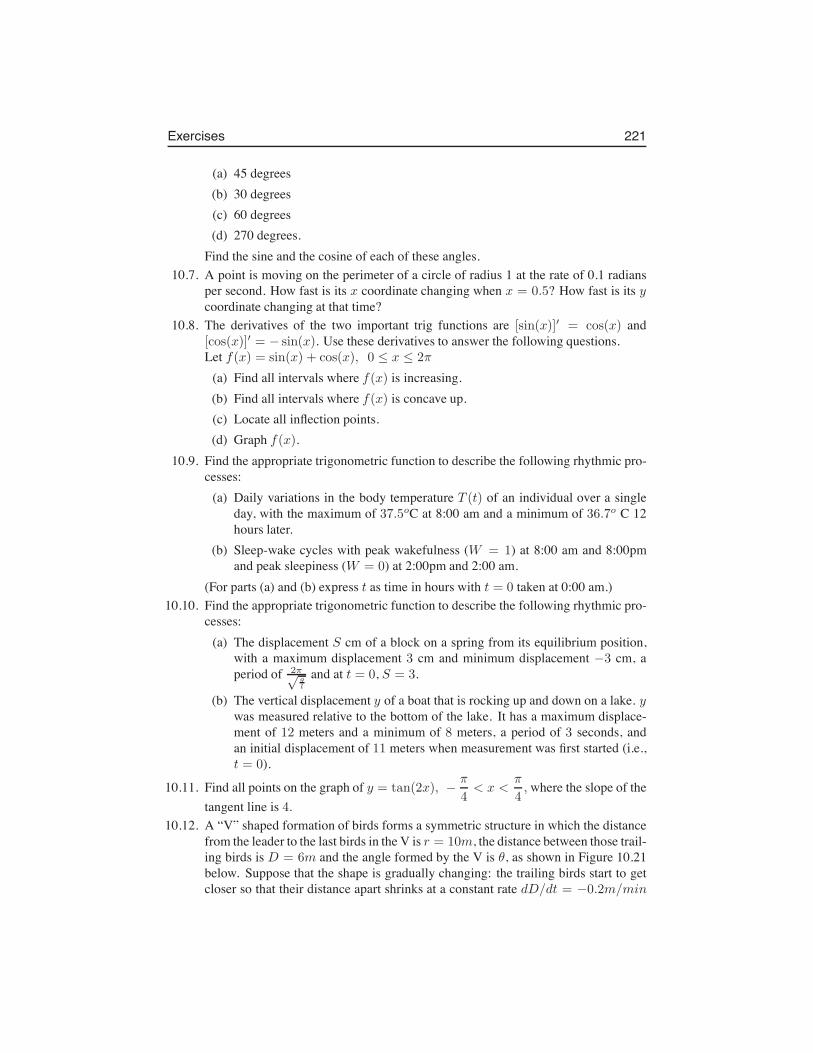
Exercises 221
(a) 45 degrees(b) 30 degrees(c) 60 degrees(d) 270 degrees.
Find the sine and the cosine of each of these angles.10.7. A point is moving on the perimeter of a circle of radius 1 at the rate of 0.1 radians
per second. How fast is its x coordinate changing when x = 0.5? How fast is its ycoordinate changing at that time?
10.8. The derivatives of the two important trig functions are [sin(x)]′ = cos(x) and[cos(x)]′ = − sin(x). Use these derivatives to answer the following questions.Let f(x) = sin(x) + cos(x), 0 ≤ x ≤ 2π
(a) Find all intervals where f(x) is increasing.(b) Find all intervals where f(x) is concave up.(c) Locate all inflection points.(d) Graph f(x).
10.9. Find the appropriate trigonometric function to describe the following rhythmic pro-cesses:
(a) Daily variations in the body temperature T (t) of an individual over a singleday, with the maximum of 37.5oC at 8:00 am and a minimum of 36.7o C 12hours later.
(b) Sleep-wake cycles with peak wakefulness (W = 1) at 8:00 am and 8:00pmand peak sleepiness (W = 0) at 2:00pm and 2:00 am.
(For parts (a) and (b) express t as time in hours with t = 0 taken at 0:00 am.)10.10. Find the appropriate trigonometric function to describe the following rhythmic pro-
cesses:(a) The displacement S cm of a block on a spring from its equilibrium position,
with a maximum displacement 3 cm and minimum displacement −3 cm, aperiod of 2π√
gl
and at t = 0, S = 3.
(b) The vertical displacement y of a boat that is rocking up and down on a lake. ywas measured relative to the bottom of the lake. It has a maximum displace-ment of 12 meters and a minimum of 8 meters, a period of 3 seconds, andan initial displacement of 11 meters when measurement was first started (i.e.,t = 0).
10.11. Find all points on the graph of y = tan(2x), −π
4< x <
π
4, where the slope of the
tangent line is 4.10.12. A “V” shaped formation of birds forms a symmetric structure in which the distance
from the leader to the last birds in the V is r = 10m, the distance between those trail-ing birds is D = 6m and the angle formed by the V is θ, as shown in Figure 10.21below. Suppose that the shape is gradually changing: the trailing birds start to getcloser so that their distance apart shrinks at a constant rate dD/dt = −0.2m/min
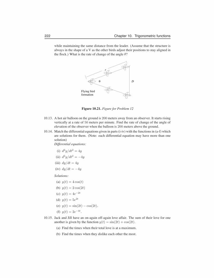
222 Chapter 10. Trigonometric functions
while maintaining the same distance from the leader. (Assume that the structure isalways in the shape of a V as the other birds adjust their positions to stay aligned inthe flock.) What is the rate of change of the angle θ?
#
Flying birdformation
D
r
Figure 10.21. Figure for Problem 12
10.13. A hot air balloon on the ground is 200 meters away from an observer. It starts risingvertically at a rate of 50 meters per minute. Find the rate of change of the angle ofelevation of the observer when the balloon is 200 meters above the ground.
10.14. Match the differential equations given in parts (i-iv) with the functions in (a-f) whichare solutions for them. (Note: each differential equation may have more than onesolution)Differential equations:
(i) d2y/dt2 = 4y
(ii) d2y/dt2 = −4y
(iii) dy/dt = 4y
(iv) dy/dt = −4y
Solutions:
(a) y(t) = 4 cos(t)
(b) y(t) = 2 cos(2t)
(c) y(t) = 4e−2t
(d) y(t) = 5e2t
(e) y(t) = sin(2t)− cos(2t),
(f) y(t) = 2e−4t.
10.15. Jack and Jill have an on-again off-again love affair. The sum of their love for oneanother is given by the function y(t) = sin(2t) + cos(2t).
(a) Find the times when their total love is at a maximum.
(b) Find the times when they dislike each other the most.
Exercises 223
10.16. A ladder of length L is leaning against a wall so that its point of contact with theground is a distance x from the wall, and its point of contact with the wall is atheight y. The ladder slips away from the wall at a constant rate C.
(a) Find an expression for the rate of change of the height y.(b) Find an expression for the rate of change of the angle θ formed between the
ladder and the wall.10.17. A cannon-ball fired by a cannon at ground level at angle θ to the horizon (0 ≤ θ ≤
π/2) will travel a horizontal distance (called the range, R) given by the formulabelow:
R =1
16v20 sin θ cos θ.
Here v0 > 0, the initial velocity of the cannon-ball, is a fixed constant and airresistance is neglected. (See Figure 10.22.) What is the maximum possible range?
R
#
Figure 10.22. Figure for problem 17
10.18. A wheel of radius 1 meter rolls on a flat surface without slipping. The wheel movesfrom left to right, rotating clockwise at a constant rate of 2 revolutions per second.Stuck to the rim of the wheel is a piece of gum, (labeled G); as the wheel rollsalong, the gum follows a path shown by the wide arc (called a “cycloid curve”) inFigure 10.23. The (x, y) coordinates of the gum (G) are related to the wheel’s angleof rotation θ by the formulae
x = θ − sin θ,
y = 1− cos θ,
where 0 ≤ θ ≤ 2π. How fast is the gum moving horizontally at the instant that itreaches its highest point? How fast is it moving vertically at that same instant?
10.19. In Figure 10.24, the point P is connected to the point O by a rod 3 cm long. Thewheel rotates around O in the clockwise direction at a constant speed, making 5revolutions per second. The point Q, which is connected to the point P by a rod 5cm long, moves along the horizontal line through O. How fast and in what directionis Q moving when P lies directly above O? (Remember the law of cosines: c2 =a2 + b2 − 2ab cos θ.)
10.20. A ship sails away from a harbor at a constant speed v. The total height of the shipincluding its mast is h. See Figure 10.25.
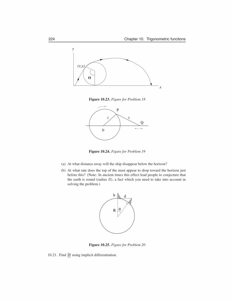
224 Chapter 10. Trigonometric functions
&
y
x
(x,y)
Figure 10.23. Figure for Problem 18
0
P
Q3 5
Figure 10.24. Figure for Problem 19
(a) At what distance away will the ship disappear below the horizon?(b) At what rate does the top of the mast appear to drop toward the horizon just
before this? (Note: In ancient times this effect lead people to conjecture thatthe earth is round (radius R), a fact which you need to take into account insolving the problem.)
R
h d
#
Figure 10.25. Figure for Problem 20
10.21. Find dydx using implicit differentiation.
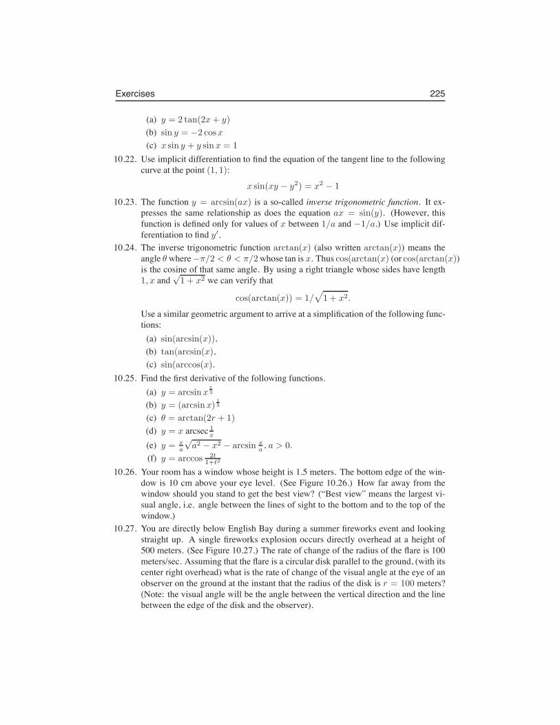
Exercises 225
(a) y = 2 tan(2x+ y)
(b) sin y = −2 cosx
(c) x sin y + y sinx = 1
10.22. Use implicit differentiation to find the equation of the tangent line to the followingcurve at the point (1, 1):
x sin(xy − y2) = x2 − 1
10.23. The function y = arcsin(ax) is a so-called inverse trigonometric function. It ex-presses the same relationship as does the equation ax = sin(y). (However, thisfunction is defined only for values of x between 1/a and −1/a.) Use implicit dif-ferentiation to find y′.
10.24. The inverse trigonometric function arctan(x) (also written arctan(x)) means theangle θ where−π/2 < θ < π/2whose tan is x. Thus cos(arctan(x) (or cos(arctan(x))is the cosine of that same angle. By using a right triangle whose sides have length1, x and
√1 + x2 we can verify that
cos(arctan(x)) = 1/√
1 + x2.
Use a similar geometric argument to arrive at a simplification of the following func-tions:
(a) sin(arcsin(x)),(b) tan(arcsin(x),(c) sin(arccos(x).
10.25. Find the first derivative of the following functions.(a) y = arcsinx
13
(b) y = (arcsinx)13
(c) θ = arctan(2r + 1)
(d) y = x arcsec 1x
(e) y = xa
√a2 − x2 − arcsin x
a , a > 0.
(f) y = arccos 2t1+t2
10.26. Your room has a window whose height is 1.5 meters. The bottom edge of the win-dow is 10 cm above your eye level. (See Figure 10.26.) How far away from thewindow should you stand to get the best view? (“Best view” means the largest vi-sual angle, i.e. angle between the lines of sight to the bottom and to the top of thewindow.)
10.27. You are directly below English Bay during a summer fireworks event and lookingstraight up. A single fireworks explosion occurs directly overhead at a height of500 meters. (See Figure 10.27.) The rate of change of the radius of the flare is 100meters/sec. Assuming that the flare is a circular disk parallel to the ground, (with itscenter right overhead) what is the rate of change of the visual angle at the eye of anobserver on the ground at the instant that the radius of the disk is r = 100 meters?(Note: the visual angle will be the angle between the vertical direction and the linebetween the edge of the disk and the observer).
226 Chapter 10. Trigonometric functions
0
#
%
x
window1.5
0.1
Figure 10.26. Figure for Problem 26
fireworks
O
#500
Figure 10.27. Figure for Problem 27
Chapter 11
Approximation methods
11.1 IntroductionIn this chapter we explore a few techniques for finding approximate solutions to problemsof great practical significance. The techniques here described are linked by a number ofcommon features; most notably, all are based on exploiting the fact that a tangent line isa good (local) approximation to the behaviour of a function (at least close to the point oftangency).
The first method, that of linear approximation has been discussed before, and is adirect application of the tangent line to approximate local behaviour of a function. We willillustrate how this approximation can lead to simple one-step computation of rough valuesthat a function of interest takes.
A second technique described here, Newton’s method, is used to find precise deci-mal approximations to zeros of a function: recall these are places where a function crossesthe x-axis, i.e. where f(x) = 0. The method gives an important example of an itera-tion scheme: that is, a recipe that is repeated (several times) to generate successively finerapproximations.
A third technique is applied to calculating numerical solutions of a differential equa-tion. This method, called Euler’s method, uses the initial condition and the differentialequation to compute approximate values of the solution step by step, starting with the ini-tial time and incrementally computing the solution value for each of many small time steps.
While some of these techniques have been superseded by improved (graphics) cal-culators, or mathematical software, the concepts behind the methods are still fundamental.Also important is understanding the limitations of such methods, since each relies on cer-tain assumptions and underlying concepts.
11.2 Linear approximationWe have already encountered the idea that the tangent line approximates the behaviour of afunction. In this technique, the approximation is used to generate rough values of a functionclose to some point at which the value of the function and of its derivative are known, or
227
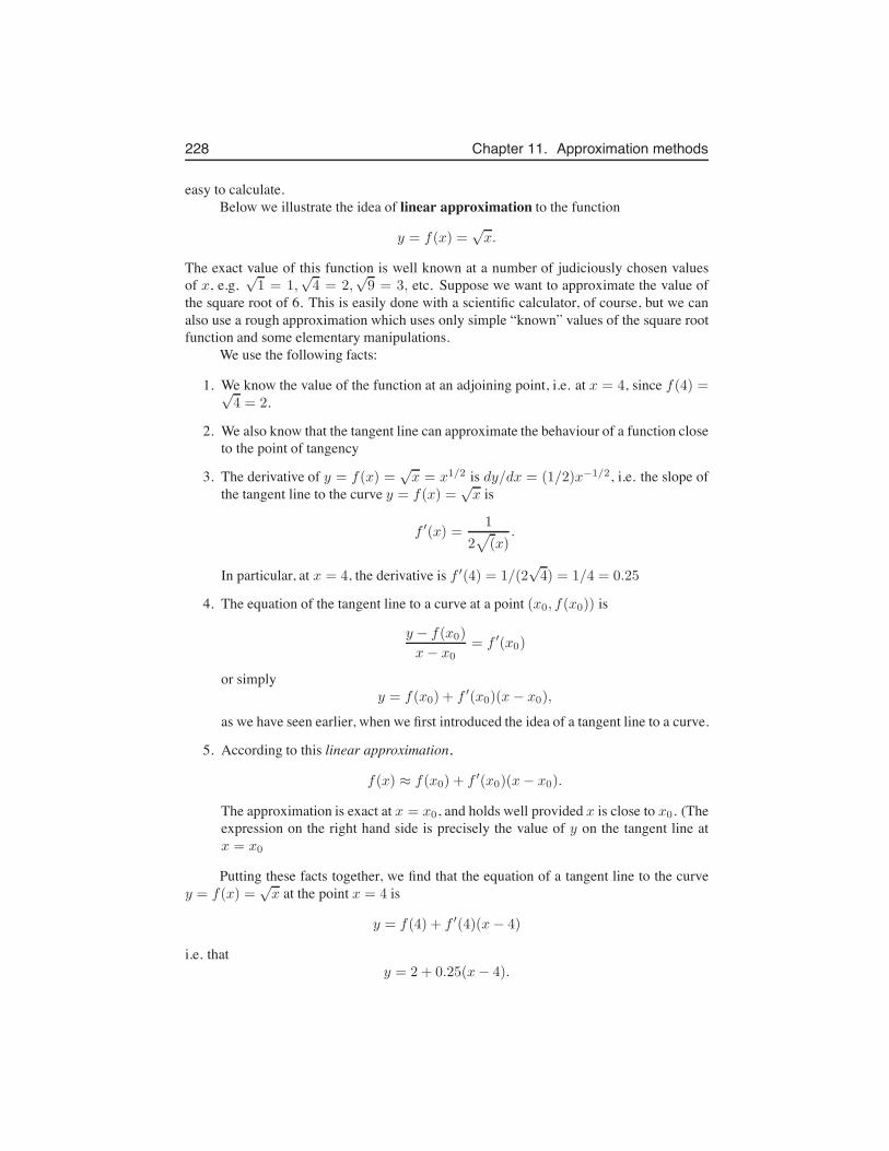
228 Chapter 11. Approximation methods
easy to calculate.Below we illustrate the idea of linear approximation to the function
y = f(x) =√x.
The exact value of this function is well known at a number of judiciously chosen valuesof x, e.g.
√1 = 1,
√4 = 2,
√9 = 3, etc. Suppose we want to approximate the value of
the square root of 6. This is easily done with a scientific calculator, of course, but we canalso use a rough approximation which uses only simple “known” values of the square rootfunction and some elementary manipulations.
We use the following facts:
1. We know the value of the function at an adjoining point, i.e. at x = 4, since f(4) =√4 = 2.
2. We also know that the tangent line can approximate the behaviour of a function closeto the point of tangency
3. The derivative of y = f(x) =√x = x1/2 is dy/dx = (1/2)x−1/2, i.e. the slope of
the tangent line to the curve y = f(x) =√x is
f ′(x) =1
2√
(x).
In particular, at x = 4, the derivative is f ′(4) = 1/(2√4) = 1/4 = 0.25
4. The equation of the tangent line to a curve at a point (x0, f(x0)) is
y − f(x0)
x− x0= f ′(x0)
or simplyy = f(x0) + f ′(x0)(x− x0),
as we have seen earlier, when we first introduced the idea of a tangent line to a curve.
5. According to this linear approximation,
f(x) ≈ f(x0) + f ′(x0)(x− x0).
The approximation is exact at x = x0, and holds well provided x is close to x0. (Theexpression on the right hand side is precisely the value of y on the tangent line atx = x0
Putting these facts together, we find that the equation of a tangent line to the curvey = f(x) =
√x at the point x = 4 is
y = f(4) + f ′(4)(x − 4)
i.e. thaty = 2 + 0.25(x− 4).
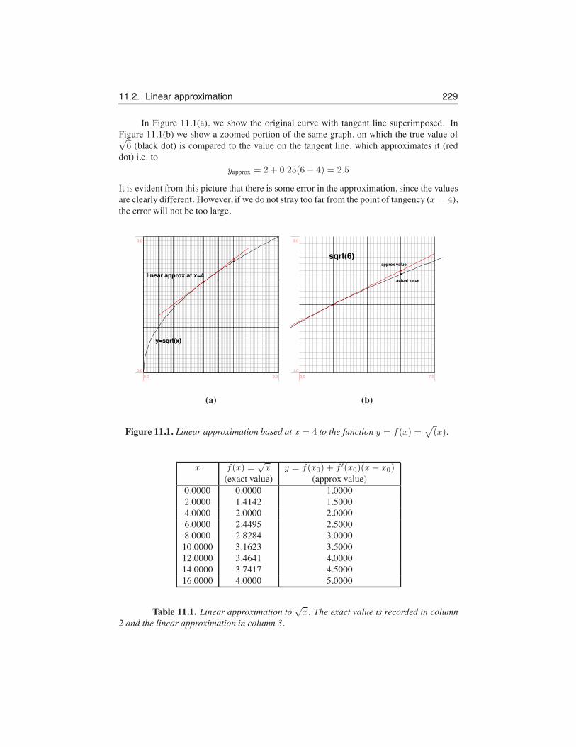
11.2. Linear approximation 229
In Figure 11.1(a), we show the original curve with tangent line superimposed. InFigure 11.1(b) we show a zoomed portion of the same graph, on which the true value of√6 (black dot) is compared to the value on the tangent line, which approximates it (red
dot) i.e. toyapprox = 2 + 0.25(6− 4) = 2.5
It is evident from this picture that there is some error in the approximation, since the valuesare clearly different. However, if we do not stray too far from the point of tangency (x = 4),the error will not be too large.
y=sqrt(x)
linear approx at x=4
0.0 9.00.0
3.0
sqrt(6)
actual value
approx value
3.0 7.01.0
3.0
(a) (b)
Figure 11.1. Linear approximation based at x = 4 to the function y = f(x) =√
(x).
x f(x) =√x y = f(x0) + f ′(x0)(x− x0)
(exact value) (approx value)0.0000 0.0000 1.00002.0000 1.4142 1.50004.0000 2.0000 2.00006.0000 2.4495 2.50008.0000 2.8284 3.0000
10.0000 3.1623 3.500012.0000 3.4641 4.000014.0000 3.7417 4.500016.0000 4.0000 5.0000
Table 11.1. Linear approximation to√x. The exact value is recorded in column
2 and the linear approximation in column 3.
230 Chapter 11. Approximation methods
In Table 11.1, we collect values of the function f(x) =√x (computed by scientific
calculator), and compare with values of the linear approximation using the tangent linethrough the point (4, 2). At x = 4, the values of the function and of its approximationare identical (naturally - since we “rigged it” to match at this point). Close the x = 4, thevalues of the approximation are fairly close to the values of the function. Further away,however, the difference between these gets bigger, and the approximation is no longer verygood at all.
These remarks illustrate two features: (1) the method is easy to use, and involves onlydetermination of a derivative, and elementary arithmetic. (2) The method has limitations,and work well only close to the point at which the tangent line is based.
11.3 Newton’s methodNewton’s method is a technique for finding approximate values for roots of an algebraicequation, that is, values of x satisfying
f(x) = 0.
(These values are also called zeros of the function f(x).) While this seems like a fairlyrestricted type of problem, actually, there are numerous applications in which this techniqueis useful, and many problems in applied and basic science that lead to such equations.We have seen that finding critical points of some function G(x), is equivalent to solvingG′(x) = 0. (i.e. if define the function of interest to be f(x) = G′(x), then we are solvingprecisely an equation of the form shown above.
We first distinguish between cases that do and do not require Newton’s method, andthen show how Newton’s method is derived and how it is used.
11.3.1 When Newton’s method is not neededExample 11.1 Find the value of x that satisfies
f(x) = 0
where f(x) = x2 + 4x+ 3.
Solution: We are asked to solve the equation
x2 + 4x+ 3 = 0.
This is a simple quadratic equation, and we have an exact formula (the quadratic formula)for the roots, i.e.
x =−4±
√
42 − 4(3)
2=
−4±√4
2= 3, 1.
In this case, we do not need Newton’s formula.
Example 11.2 Find values of x for which sin(x) = 1.
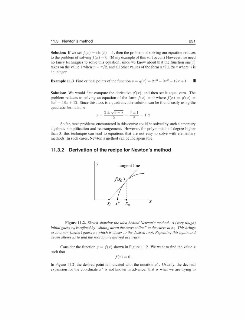
11.3. Newton’s method 231
Solution: If we set f(x) = sin(x) − 1, then the problem of solving our equation reducesto the problem of solving f(x) = 0. (Many example of this sort occur.) However, we needno fancy techniques to solve this equation, since we know about that the function sin(x)takes on the value 1 when x = π/2, and all other values of the form π/2± 2nπ where n isan integer.
Example 11.3 Find critical points of the function y = g(x) = 2x3 − 9x2 + 12x+ 1.
Solution: We would first compute the derivative g′(x), and then set it equal zero. Theproblem reduces to solving an equation of the form f(x) = 0 where f(x) = g′(x) =6x2 − 18x + 12. Since this, too, is a quadratic, the solution can be found easily using thequadratic formula, i.e.
x =3±
√9− 8
2=
3± 1
2= 1, 2
So far, most problems encountered in this course could be solved by such elementaryalgebraic simplification and rearrangement. However, for polynomials of degree higherthan 3, this technique can lead to equations that are not easy to solve with elementarymethods. In such cases, Newton’s method can be indispensable.
11.3.2 Derivation of the recipe for Newton’s method
x
y
x
f(x )
x x* 01
0
tangent line
Figure 11.2. Sketch showing the idea behind Newton’s method. A (very rough)initial guess x0 is refined by “sliding down the tangent line” to the curve at x0. This bringsus to a new (better) guess x1 which is closer to the desired root. Repeating this again andagain allows us to find the root to any desired accuracy.
Consider the function y = f(x) shown in Figure 11.2. We want to find the value xsuch that
f(x) = 0.
In Figure 11.2, the desired point is indicated with the notation x∗. Usually, the decimalexpansion for the coordinate x∗ is not known in advance: that is what we are trying to
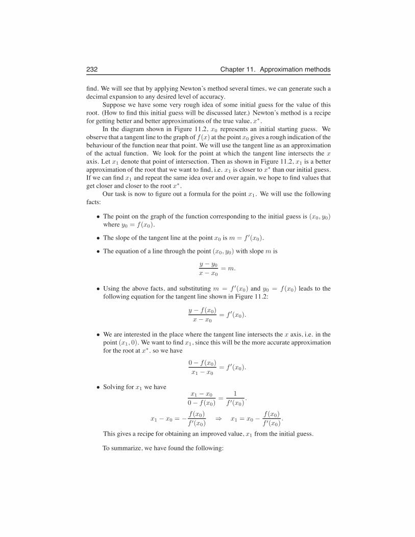
232 Chapter 11. Approximation methods
find. We will see that by applying Newton’s method several times, we can generate such adecimal expansion to any desired level of accuracy.
Suppose we have some very rough idea of some initial guess for the value of thisroot. (How to find this initial guess will be discussed later.) Newton’s method is a recipefor getting better and better approximations of the true value, x∗.
In the diagram shown in Figure 11.2, x0 represents an initial starting guess. Weobserve that a tangent line to the graph of f(x) at the pointx0 gives a rough indication of thebehaviour of the function near that point. We will use the tangent line as an approximationof the actual function. We look for the point at which the tangent line intersects the xaxis. Let x1 denote that point of intersection. Then as shown in Figure 11.2, x1 is a betterapproximation of the root that we want to find, i.e. x1 is closer to x∗ than our initial guess.If we can find x1 and repeat the same idea over and over again, we hope to find values thatget closer and closer to the root x∗.
Our task is now to figure out a formula for the point x1. We will use the followingfacts:
• The point on the graph of the function corresponding to the initial guess is (x0, y0)where y0 = f(x0).
• The slope of the tangent line at the point x0 is m = f ′(x0).
• The equation of a line through the point (x0, y0) with slope m is
y − y0x− x0
= m.
• Using the above facts, and substituting m = f ′(x0) and y0 = f(x0) leads to thefollowing equation for the tangent line shown in Figure 11.2:
y − f(x0)
x− x0= f ′(x0).
• We are interested in the place where the tangent line intersects the x axis, i.e. in thepoint (x1, 0). We want to find x1, since this will be the more accurate approximationfor the root at x∗. so we have
0− f(x0)
x1 − x0= f ′(x0).
• Solving for x1 we havex1 − x0
0− f(x0)=
1
f ′(x0).
x1 − x0 = −f(x0)
f ′(x0)⇒ x1 = x0 −
f(x0)
f ′(x0).
This gives a recipe for obtaining an improved value, x1 from the initial guess.
To summarize, we have found the following:
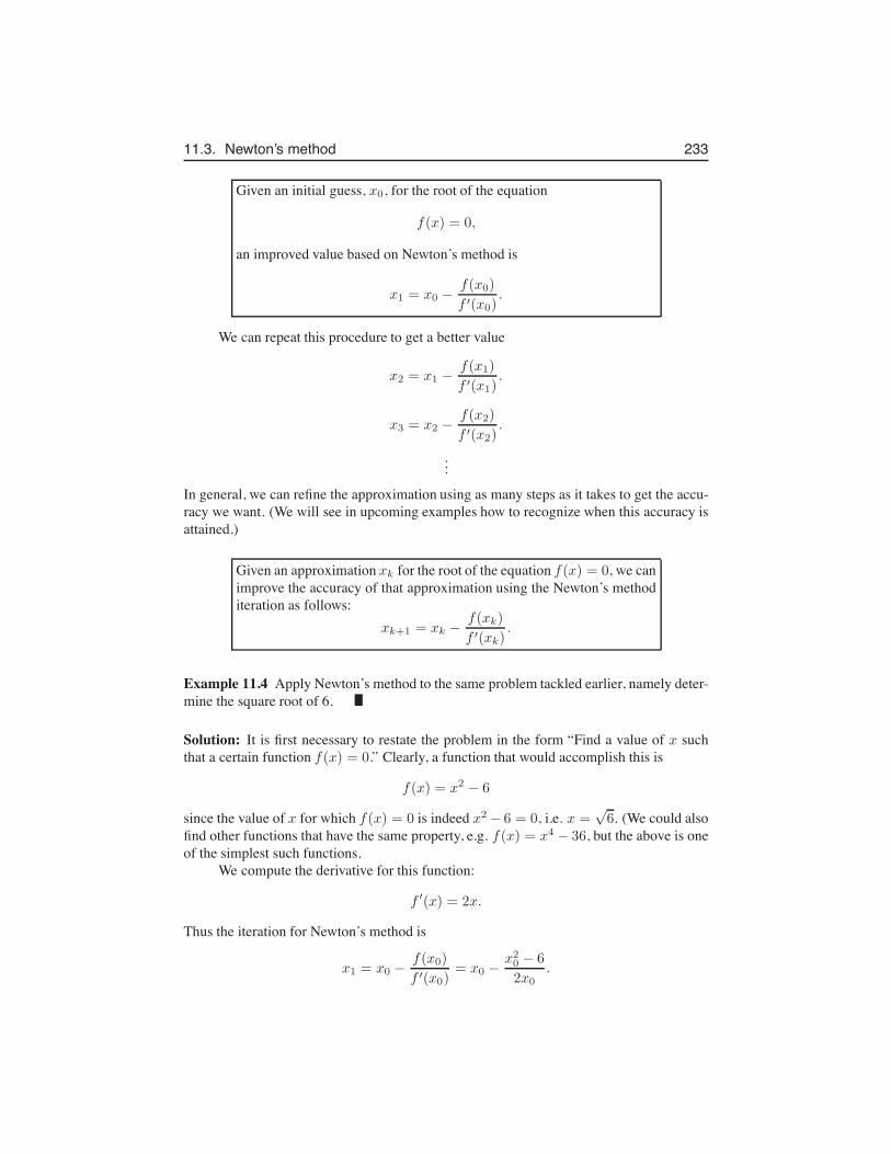
11.3. Newton’s method 233
Given an initial guess, x0, for the root of the equation
f(x) = 0,
an improved value based on Newton’s method is
x1 = x0 −f(x0)
f ′(x0).
We can repeat this procedure to get a better value
x2 = x1 −f(x1)
f ′(x1).
x3 = x2 −f(x2)
f ′(x2).
...
In general, we can refine the approximation using as many steps as it takes to get the accu-racy we want. (We will see in upcoming examples how to recognize when this accuracy isattained.)
Given an approximation xk for the root of the equation f(x) = 0, we canimprove the accuracy of that approximation using the Newton’s methoditeration as follows:
xk+1 = xk −f(xk)
f ′(xk).
Example 11.4 Apply Newton’s method to the same problem tackled earlier, namely deter-mine the square root of 6.
Solution: It is first necessary to restate the problem in the form “Find a value of x suchthat a certain function f(x) = 0.” Clearly, a function that would accomplish this is
f(x) = x2 − 6
since the value of x for which f(x) = 0 is indeed x2 − 6 = 0, i.e. x =√6. (We could also
find other functions that have the same property, e.g. f(x) = x4 − 36, but the above is oneof the simplest such functions.
We compute the derivative for this function:
f ′(x) = 2x.
Thus the iteration for Newton’s method is
x1 = x0 −f(x0)
f ′(x0)= x0 −
x20 − 6
2x0.
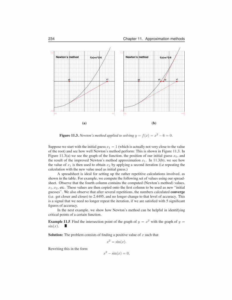
234 Chapter 11. Approximation methods
x0 x1
Newton’s method f(x)=x^2-6
0.0 4.0-7.0
7.0
x0 x1
Newton’s method f(x)=x^2-6
x2x3
0.0 4.0-7.0
7.0
(a) (b)
Figure 11.3. Newton’s method applied to solving y = f(x) = x2 − 6 = 0.
Suppose we start with the initial guess x1 = 1 (which is actually not very close to the valueof the root) and see how well Newton’s method perform: This is shown in Figure 11.3. InFigure 11.3(a) we see the graph of the function, the position of our initial guess x0, andthe result of the improved Newton’s method approximation x1. In 11.3(b), we see howthe value of x1 is then used to obtain x2 by applying a second iteration (i.e repeating thecalculation with the new value used as initial guess.)
A spreadsheet is ideal for setting up the rather repetitive calculations involved, asshown in the table. For example, we compute the following set of values using our spread-sheet. Observe that the fourth column contains the computed (Newton’s method) values,x1, x2, etc. These values are then copied onto the first column to be used as new “initialguesses”. We also observe that after several repetitions, the numbers calculated converge(i.e. get closer and closer) to 2.4495, and no longer change to that level of accuracy. Thisis a signal that we need no longer repeat the iteration, if we are satisfied with 5 significantfigures of accuracy.
In the next example, we show how Newton’s method can be helpful in identifyingcritical points of a certain function.
Example 11.5 Find the intersection point of the graph of y = x2 with the graph of y =sin(x).
Solution: The problem consists of finding a positive value of x such that
x2 = sin(x).
Rewriting this in the formx2 − sin(x) = 0,
11.3. Newton’s method 235
k xk f(xk) f ′(xk) xk+1
0 1.00 -5.00 2.00 3.51 3.5 6.250 7.00 2.60712 2.6071 0.7972 5.2143 2.45433 2.4543 0.0234 4.9085 2.44954 2.4495 0.000 4.8990 2.4495
Table 11.2. Newton’s method applied to Example 11.4. We start with x0 = 1 asour initial approximation and refine it four times.
we recognize a problem of the sort that Newton’s method can solve. We let f(x) = x2 −sin(x), and look for roots of f(x) = 0.
To start, we observe that for x0 = 1 it is true that x2 = 1, and sin(x) ≈ x ≈ 1. Thissuggests that we could use the initial guess x0 = 1.
We havef(x) = x2 − sin(x),
sof ′(x) = 2x− cos(x).
and thusx1 = x0 −
f(x0)
f ′(x0)= x0 −
x20 − sin(x0)
2x0 − cos(x0).
Sox1 = 1−
1− sin(1)
2− cos(1)= 1−
1− 0.8414
2− 0.54= 0.8914
We then evaluate
x2 = x1 −f(x1)
f ′(x1)= x1 −
x21 − sin(x1)
2x1 − cos(x1)= 0.8770.
We similarly find thatx3 = 0.8767,
x4 = 0.8767.
Thus, the sequence of values converges easily to the value of the root after only threerepetitions.
Example 11.6 Find a critical point of the function y = x3 + e−x.
Solution: The function is shown in Figure 11.4. We must turn this into the appropriateproblem to which Newton’s method will apply. The critical points of this function arevalues of x such that
dy
dx= 3x2 − e−x = 0.
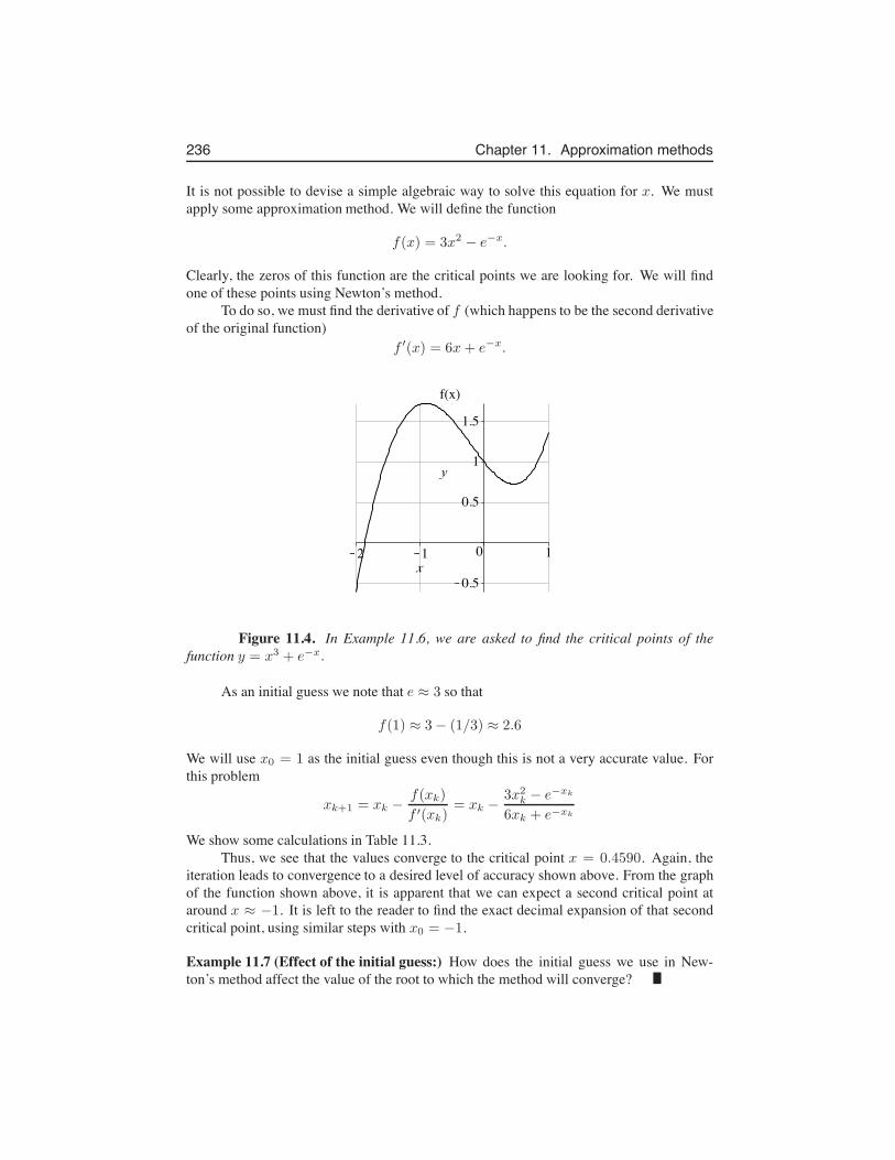
236 Chapter 11. Approximation methods
It is not possible to devise a simple algebraic way to solve this equation for x. We mustapply some approximation method. We will define the function
f(x) = 3x2 − e−x.
Clearly, the zeros of this function are the critical points we are looking for. We will findone of these points using Newton’s method.
To do so, we must find the derivative of f (which happens to be the second derivativeof the original function)
f ′(x) = 6x+ e−x.
Figure 11.4. In Example 11.6, we are asked to find the critical points of thefunction y = x3 + e−x.
As an initial guess we note that e ≈ 3 so that
f(1) ≈ 3− (1/3) ≈ 2.6
We will use x0 = 1 as the initial guess even though this is not a very accurate value. Forthis problem
xk+1 = xk −f(xk)
f ′(xk)= xk −
3x2k − e−xk
6xk + e−xk
We show some calculations in Table 11.3.Thus, we see that the values converge to the critical point x = 0.4590. Again, the
iteration leads to convergence to a desired level of accuracy shown above. From the graphof the function shown above, it is apparent that we can expect a second critical point ataround x ≈ −1. It is left to the reader to find the exact decimal expansion of that secondcritical point, using similar steps with x0 = −1.
Example 11.7 (Effect of the initial guess:) How does the initial guess we use in New-ton’s method affect the value of the root to which the method will converge?
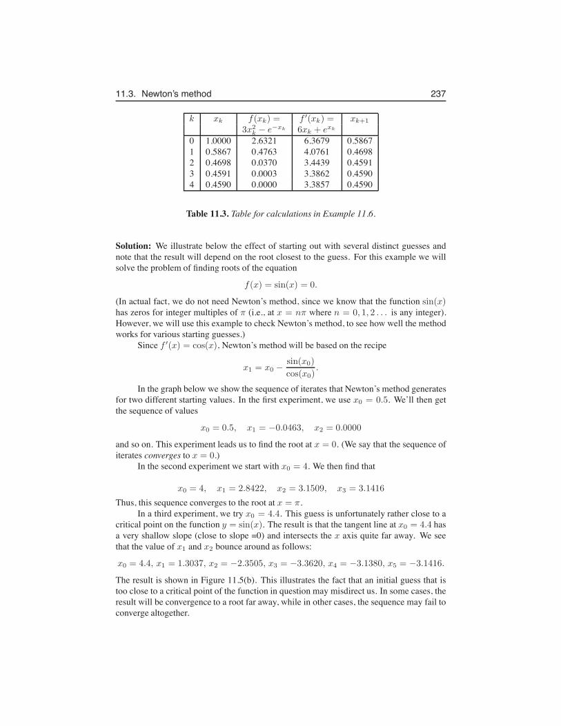
11.3. Newton’s method 237
k xk f(xk) = f ′(xk) = xk+1
3x2k − e−xk 6xk + exk
0 1.0000 2.6321 6.3679 0.58671 0.5867 0.4763 4.0761 0.46982 0.4698 0.0370 3.4439 0.45913 0.4591 0.0003 3.3862 0.45904 0.4590 0.0000 3.3857 0.4590
Table 11.3. Table for calculations in Example 11.6.
Solution: We illustrate below the effect of starting out with several distinct guesses andnote that the result will depend on the root closest to the guess. For this example we willsolve the problem of finding roots of the equation
f(x) = sin(x) = 0.
(In actual fact, we do not need Newton’s method, since we know that the function sin(x)has zeros for integer multiples of π (i.e., at x = nπ where n = 0, 1, 2 . . . is any integer).However, we will use this example to check Newton’s method, to see how well the methodworks for various starting guesses.)
Since f ′(x) = cos(x), Newton’s method will be based on the recipe
x1 = x0 −sin(x0)
cos(x0).
In the graph below we show the sequence of iterates that Newton’s method generatesfor two different starting values. In the first experiment, we use x0 = 0.5. We’ll then getthe sequence of values
x0 = 0.5, x1 = −0.0463, x2 = 0.0000
and so on. This experiment leads us to find the root at x = 0. (We say that the sequence ofiterates converges to x = 0.)
In the second experiment we start with x0 = 4. We then find that
x0 = 4, x1 = 2.8422, x2 = 3.1509, x3 = 3.1416
Thus, this sequence converges to the root at x = π.In a third experiment, we try x0 = 4.4. This guess is unfortunately rather close to a
critical point on the function y = sin(x). The result is that the tangent line at x0 = 4.4 hasa very shallow slope (close to slope =0) and intersects the x axis quite far away. We seethat the value of x1 and x2 bounce around as follows:
x0 = 4.4, x1 = 1.3037, x2 = −2.3505, x3 = −3.3620, x4 = −3.1380, x5 = −3.1416.
The result is shown in Figure 11.5(b). This illustrates the fact that an initial guess that istoo close to a critical point of the function in question may misdirect us. In some cases, theresult will be convergence to a root far away, while in other cases, the sequence may fail toconverge altogether.
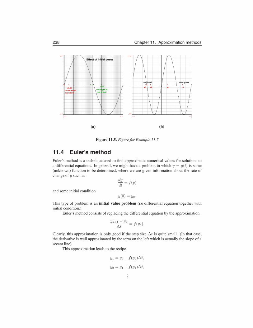
238 Chapter 11. Approximation methods
x0=0.5converges toroot at x=0
x0=4converges toroot at x=pi
Effect of initial guess
-0.1 6.3-1.0
1.0
x0x1x2x3
initial guessroot found
-6.3 6.3-1.0
1.0
(a) (b)
Figure 11.5. Figure for Example 11.7
11.4 Euler’s methodEuler’s method is a technique used to find approximate numerical values for solutions toa differential equations. In general, we might have a problem in which y = g(t) is some(unknown) function to be determined, where we are given information about the rate ofchange of y such as
dy
dt= f(y)
and some initial conditiony(0) = y0.
This type of problem is an initial value problem (i.e differential equation together withinitial condition.)
Euler’s method consists of replacing the differential equation by the approximation
yk+1 − yk∆t
= f(yk).
Clearly, this approximation is only good if the step size ∆t is quite small. (In that case,the derivative is well approximated by the term on the left which is actually the slope of asecant line)
This approximation leads to the recipe
y1 = y0 + f(y0)∆t,
y2 = y1 + f(y1)∆t,
...
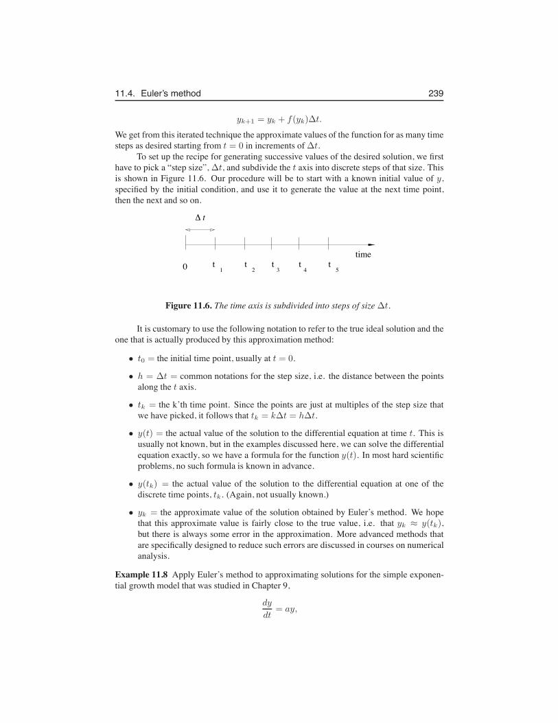
11.4. Euler’s method 239
yk+1 = yk + f(yk)∆t.
We get from this iterated technique the approximate values of the function for as many timesteps as desired starting from t = 0 in increments of ∆t.
To set up the recipe for generating successive values of the desired solution, we firsthave to pick a “step size”, ∆t, and subdivide the t axis into discrete steps of that size. Thisis shown in Figure 11.6. Our procedure will be to start with a known initial value of y,specified by the initial condition, and use it to generate the value at the next time point,then the next and so on.
time
' t
t t t t t0 1 2 3 4 5
Figure 11.6. The time axis is subdivided into steps of size ∆t.
It is customary to use the following notation to refer to the true ideal solution and theone that is actually produced by this approximation method:
• t0 = the initial time point, usually at t = 0.
• h = ∆t = common notations for the step size, i.e. the distance between the pointsalong the t axis.
• tk = the k’th time point. Since the points are just at multiples of the step size thatwe have picked, it follows that tk = k∆t = h∆t.
• y(t) = the actual value of the solution to the differential equation at time t. This isusually not known, but in the examples discussed here, we can solve the differentialequation exactly, so we have a formula for the function y(t). In most hard scientificproblems, no such formula is known in advance.
• y(tk) = the actual value of the solution to the differential equation at one of thediscrete time points, tk. (Again, not usually known.)
• yk = the approximate value of the solution obtained by Euler’s method. We hopethat this approximate value is fairly close to the true value, i.e. that yk ≈ y(tk),but there is always some error in the approximation. More advanced methods thatare specifically designed to reduce such errors are discussed in courses on numericalanalysis.
Example 11.8 Apply Euler’s method to approximating solutions for the simple exponen-tial growth model that was studied in Chapter 9,
dy
dt= ay,
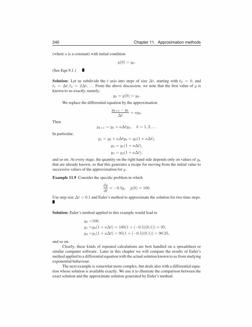
240 Chapter 11. Approximation methods
(where a is a constant) with initial condition
y(0) = y0.
(See Eqn 9.1.)
Solution: Let us subdivide the t axis into steps of size ∆t, starting with t0 = 0, andt1 = ∆t, t2 = 2∆t, . . . From the above discussion, we note that the first value of y isknown to us exactly, namely,
y0 = y(0) = y0.
We replace the differential equation by the approximation
yk+1 − yk∆t
= ayk.
Thenyk+1 = yk + a∆tyk, k = 1, 2, . . .
In particular,y1 = y0 + a∆ty0 = y0(1 + a∆t),
y2 = y1(1 + a∆t),
y3 = y2(1 + a∆t),
and so on. At every stage, the quantity on the right hand side depends only on values of ykthat are already known, so that this generates a recipe for moving from the initial value tosuccessive values of the approximation for y.
Example 11.9 Consider the specific problem in which
dy
dt= −0.5y, y(0) = 100.
Use step size ∆t = 0.1 and Euler’s method to approximate the solution for two time steps.
Solution: Euler’s method applied to this example would lead to
y0 =100.
y1 =y0(1 + a∆t) = 100(1 + (−0.5)(0.1)) = 95,
y2 =y1(1 + a∆t) = 95(1 + (−0.5)(0.1)) = 90.25,
and so on.Clearly, these kinds of repeated calculations are best handled on a spreadsheet or
similar computer software. Later in this chapter we will compare the results of Euler’smethod applied to a differential equation with the actual solution known to us from studyingexponential behaviour.
The next example is somewhat more complex, but deals also with a differential equa-tion whose solution is available exactly. We use it to illustrate the comparison between theexact solution and the approximate solution generated by Euler’s method.
11.4. Euler’s method 241
11.4.1 Applying Euler’s method to Newton’s law of coolingWe apply Euler’s method to the differential equation that describes the cooling of an object.(This differential equation is called Newton’s Law of Cooling, though it is unrelated to theNewton’s method we investigated above.) According to Newton,
The rate of change of temperature T of an object is proportionalto the difference between its temperature and the ambient tempera-ture, E.
This hypothesis about the way that temperature T (t) changes leads to the differentialequation
dT
dt= k(E − T ).
Suppose we are given an initial condition that prescribes the temperature at the beginningof the observation, T (0) = T0. This initial value problem has a solution that can be writtenin a simple formula, i.e.
T (t) = E + (T0 − E)e−kt.
(See Chapter 12 for a derivation of this result.) We will refer to this formula, which holdsexactly for all values of time t as the true solution. Observe that it is some function oftime that gives a full record of the behaviour of the temperature of the object as it coolsoff or heats up in its environment. However, the numerical values of temperature at agiven time still need to be plotted or computed for this formula to be useful quantitatively.This motivates us to look for some approximate technique that would use the differentialequation and the initial condition directly to plot quantitative behaviour, without the needfor a formula for the solution, T (t).
Example 11.10 (Newton’s law of cooling:) For simplicity, consider the case that the am-bient temperature is E = 10 degrees. Suppose that the constant k is k = 0.2. Find theexact solution, that is, determine the (formula for) the temperature as a function of timeT (t).
Solution: In this case, the differential equation has the form
dT
dt= 0.2(10− T ),
and its solution (which is known exactly) is
T (t) = 10 + (T0 − 10)e−0.2t.
We will investigate the solutions from several initial conditions, T (0) = 0, 5, 15, 20 de-grees.
Example 11.11 (Euler’s method applied to Newton’s law of cooling:) Write down the Eu-ler’s method formula that can be used to find an approximation to the solution of Exam-ple 11.10
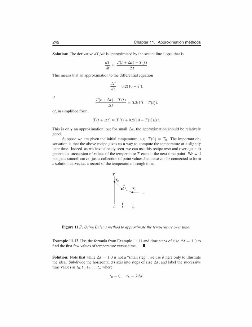
242 Chapter 11. Approximation methods
Solution: The derivative dT/dt is approximated by the secant line slope, that is
dT
dt≈
T (t+∆t)− T (t)
∆t.
This means that an approximation to the differential equation
dT
dt= 0.2(10− T ),
isT (t+∆t)− T (t)
∆t= 0.2(10− T (t)).
or, in simplified form,
T (t+∆t) ≈ T (t) + 0.2(10− T (t))∆t.
This is only an approximation, but for small ∆t, the approximation should be relativelygood.
Suppose we are given the initial temperature, e.g. T (0) = T0. The important ob-servation is that the above recipe gives us a way to compute the temperature at a slightlylater time. Indeed, as we have already seen, we can use this recipe over and over again togenerate a succession of values of the temperature T each at the next time point. We willnot get a smooth curve: just a collection of point values, but these can be connected to forma solution curve, i.e. a record of the temperature through time.
T
T
TT
0 t t
12
0
1 2
Figure 11.7. Using Euler’s method to approximate the temperature over time.
Example 11.12 Use the formula from Example 11.11 and time steps of size ∆t = 1.0 tofind the first few values of temperature versus time.
Solution: Note that while ∆t = 1.0 is not a “small step”, we use it here only to illustratethe idea. Subdivide the horizontal (t) axis into steps of size ∆t, and label the successivetime values as t0, t1, t2, . . . tn where
t0 = 0, tk = k∆t.
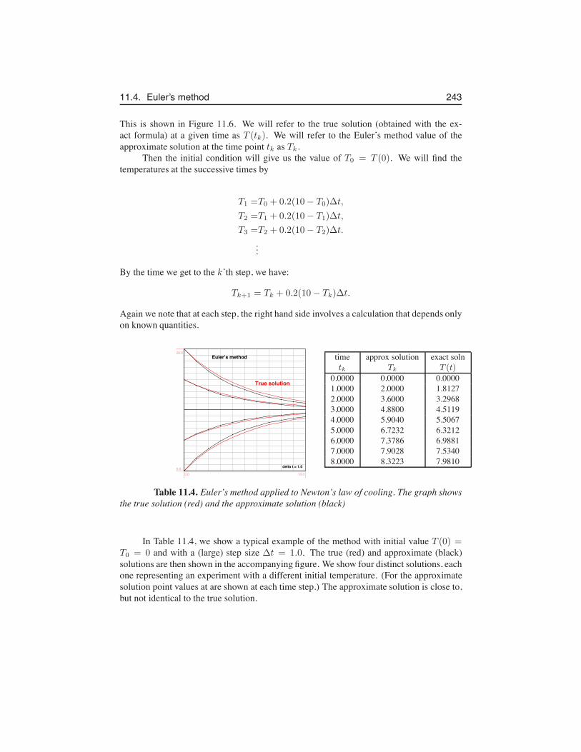
11.4. Euler’s method 243
This is shown in Figure 11.6. We will refer to the true solution (obtained with the ex-act formula) at a given time as T (tk). We will refer to the Euler’s method value of theapproximate solution at the time point tk as Tk.
Then the initial condition will give us the value of T0 = T (0). We will find thetemperatures at the successive times by
T1 =T0 + 0.2(10− T0)∆t,
T2 =T1 + 0.2(10− T1)∆t,
T3 =T2 + 0.2(10− T2)∆t.
...
By the time we get to the k’th step, we have:
Tk+1 = Tk + 0.2(10− Tk)∆t.
Again we note that at each step, the right hand side involves a calculation that depends onlyon known quantities.
delta t = 1.0
Euler’s method
True solution
0.0 10.00.0
20.0time approx solution exact solntk Tk T (t)
0.0000 0.0000 0.00001.0000 2.0000 1.81272.0000 3.6000 3.29683.0000 4.8800 4.51194.0000 5.9040 5.50675.0000 6.7232 6.32126.0000 7.3786 6.98817.0000 7.9028 7.53408.0000 8.3223 7.9810
Table 11.4. Euler’s method applied to Newton’s law of cooling. The graph showsthe true solution (red) and the approximate solution (black)
In Table 11.4, we show a typical example of the method with initial value T (0) =T0 = 0 and with a (large) step size ∆t = 1.0. The true (red) and approximate (black)solutions are then shown in the accompanying figure. We show four distinct solutions, eachone representing an experiment with a different initial temperature. (For the approximatesolution point values at are shown at each time step.) The approximate solution is close to,but not identical to the true solution.
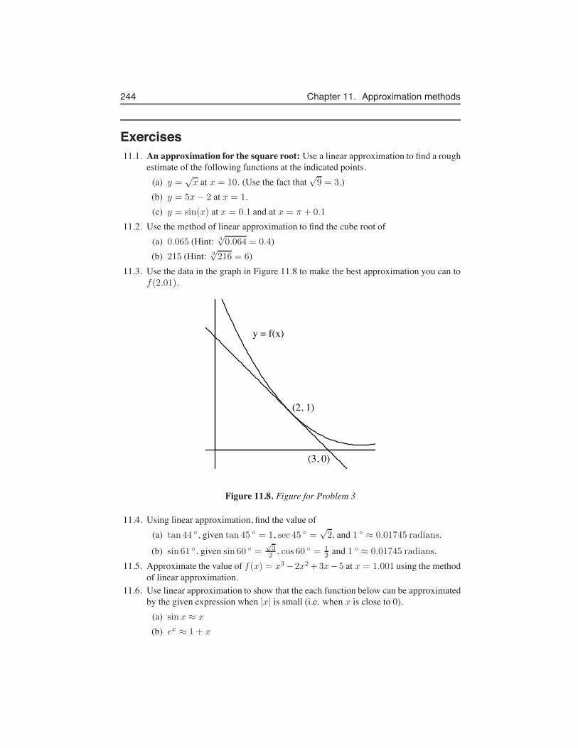
244 Chapter 11. Approximation methods
Exercises11.1. An approximation for the square root: Use a linear approximation to find a rough
estimate of the following functions at the indicated points.(a) y =
√x at x = 10. (Use the fact that
√9 = 3.)
(b) y = 5x− 2 at x = 1.(c) y = sin(x) at x = 0.1 and at x = π + 0.1
11.2. Use the method of linear approximation to find the cube root of(a) 0.065 (Hint: 3
√0.064 = 0.4)
(b) 215 (Hint: 3√216 = 6)
11.3. Use the data in the graph in Figure 11.8 to make the best approximation you can tof(2.01).
(2, 1)
(3, 0)
y = f(x)
Figure 11.8. Figure for Problem 3
11.4. Using linear approximation, find the value of(a) tan 44 ◦, given tan 45 ◦ = 1, sec 45 ◦ =
√2, and 1 ◦ ≈ 0.01745 radians.
(b) sin 61 ◦, given sin 60 ◦ =√32 , cos 60 ◦ = 1
2 and 1 ◦ ≈ 0.01745 radians.11.5. Approximate the value of f(x) = x3−2x2+3x−5 at x = 1.001 using the method
of linear approximation.11.6. Use linear approximation to show that the each function below can be approximated
by the given expression when |x| is small (i.e. when x is close to 0).(a) sinx ≈ x
(b) ex ≈ 1 + x
Exercises 245
(c) ln(1 + x) ≈ x
11.7. Approximate the volume of a cube whose length of each side is 10.1 cm.11.8. Finding critical points: Use Newton’s method to find critical points of the function
y = ex − 2x2
11.9. Estimating a square root: Use Newton’s method to find an approximate value for√8. (Hint: First think of a function, f(x), such that f(x) = 0 has the solution
x =√8).
11.10. Finding points of intersection: Find the point(s) of intersection of:
(a) y1 = 8x3 − 10x2 + x+ 2 and y2 = x3 + 15x2 − x− 4 (Hint: an intersectionpoint exists between x = 3 and x = 4).
(b) y1 = e−x and y2 = lnx
11.11. Roots of cubic equations: Find the roots for each of the following cubic equationsusing Newton’s method:
(a) x3 + 3x− 1 = 0
(b) x3 + x2 + x− 2 = 0
(c) x3+5x2−2 = 0 (Hint: Find an approximation to a first root a using Newton’smethod, then divide the left hand side of the equation by (x − a) to obtain aquadratic equation, which can be solved by the quadratic formula.)
(d) f(x) = x ln x and g(x) = 2 (find the larger root only)
11.12. Use Newton’s method to find an approximation (correct to ±0.01 ) for any roots ofthe equation
sin(x) =1
2x
How many roots does this equation actually have ? Draw a diagram showing thefunctions y = sin(x) and y = x/2 on the same set of axes to help answer thisquestion.
11.13. More critical points: Let f(x) = (x2 + x− 1)e−x2 .
(a) Find all critical points of f(x) and indicate whether each one is a local maxi-mum, local minimum, or neither.
(b) Graph f(x). Indicate the regions where f ′′(x) is positive.
11.14. Use Newton’s method to find a value of x that satisfies
ex − x2/2 = 0 .
Use the starting value x0 = 0. Display your answer to 4 significant figures.11.15. We will use Newton’s method to investigate zeros of the function
y = f(x) = sin(x)− e−x
(i.e. roots of the equation f(x) = 0.)
246 Chapter 11. Approximation methods
(a) Use the spreadsheet to graph the function
f(x) = sin(x)− exp(−x)
for values of x from 0 up to 6.(b) Find the equation of the tangent line to the curve at the point x0 = 1 and plot
it on the same graph.(c) Use the value x0 = 1 as an initial guess, and apply Newton’s method. Plot
the values (x1, 0), (x2, 0), and (x3, 0) on the same graph produced by yourspreadsheet to show how the points approach the zero of the function. Use thismethod to find the value of the root to four significant figures.
(d) Use a separate computation with the spreadsheet to determine the value of theroot you find with the starting guess x0 = 4. (You need not show this on thegraph). Do you get to the same value as you did in part (c)? Why or why not?
(e) This function has lots of zeros. From your familiarity with the functions sin(x)and e−x, where do you expect to find the roots for larger x values?Hand in a graph produced by the spreadsheet, and an additional page showingany calculations you made to get the answers. You can print the spreadsheetcontents as part of your hand-in work.
11.16. Comparing approximate and true solutions:(a) Use Euler’s method to find an approximate solution to the differential equation
dy
dx= y
with y(0) = 1. Use a step size h = 0.1 and find the values of y up to x =0.5. Compare the value you have calculated for y(0.5) using Euler’s methodwith the true solution of this differential equation. What is the error i.e. thedifference between the true solution and the approximation?
(b) Now use Euler’s method on the differential equation
dy
dx= −y
with y(0) = 1. Use a step size h = 0.1 again and find the values of y upto x = 0.5. Compare the value you have calculated for y(0.5) using Euler’smethod with the true solution of this differential equation. What is the errorthis time?
11.17. Euler’s method applied to logistic growth: Consider the logistic differential equa-tion
dy
dt= ry(1 − y)
Let r = 1. Use Euler’s method to find a solution to this differential equation startingwith y(0) = 0.5, and step size h = 0.2. Find the values of y up to time t = 1.0.
Exercises 247
11.18. Use the spreadsheet and Euler’s method to solve the differential equation shownbelow:
dy/dt = 0.5y(2− y)
Use a step size of h = 0.1 and show (on the same graph) solutions for the followingfour initial values:
y(0) = 0.5, y(0) = 1, y(0) = 1.5, y(0) = 2.25
For full credit, you must include a short explanation of what you did (e.g. 1-2sentences and whatever equations you implemented on the spreadsheet.)
11.19. Other differential equations: For each of the following differential equations, findthe approximate solution by Euler’s method in the specified interval using the giveninitial condition and step size (display three decimal places for your answer).
(a) dy
dx= y, y(0) = 1
2 . Find the five successive values of y(x) using a step sizeof step size ∆x = h = 0.1. (your values will correspond to points along theinterval 0 < x < 0.5).
(b) dy
dx= x + y, y(0) = 1, step size 0.1 on the interval [−0.5, 0]. (Note: starting
at x = 0, you are going in the negative x direction.)
(c) dy
dx=
√x+ y, y(1) = 2, find y on [1, 2] in 5 steps.
11.20. For each of the following differential equations, find value of y at the specific pointby Euler’s method using the given initial condition and step size (display three dec-imal places for your answer).
(a) dy
dx= x+ y2, y(0) = 1, step size h = 0.02, find y(0.1).
(b) dy
dx=
√
x2 + y2, y(0.2) = 0.5, find y(0.4) in 4 steps.

248 Chapter 11. Approximation methods
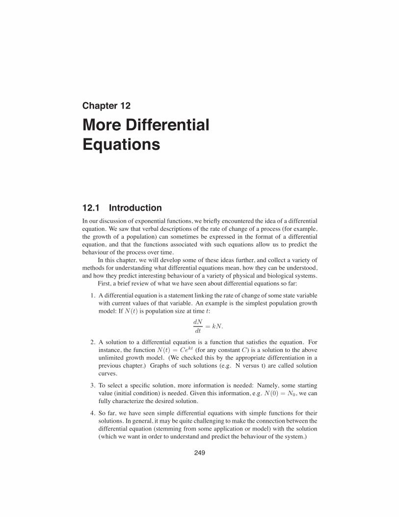
Chapter 12
More DifferentialEquations
12.1 IntroductionIn our discussion of exponential functions, we briefly encountered the idea of a differentialequation. We saw that verbal descriptions of the rate of change of a process (for example,the growth of a population) can sometimes be expressed in the format of a differentialequation, and that the functions associated with such equations allow us to predict thebehaviour of the process over time.
In this chapter, we will develop some of these ideas further, and collect a variety ofmethods for understanding what differential equations mean, how they can be understood,and how they predict interesting behaviour of a variety of physical and biological systems.
First, a brief review of what we have seen about differential equations so far:
1. A differential equation is a statement linking the rate of change of some state variablewith current values of that variable. An example is the simplest population growthmodel: If N(t) is population size at time t:
dN
dt= kN.
2. A solution to a differential equation is a function that satisfies the equation. Forinstance, the function N(t) = Cekt (for any constant C) is a solution to the aboveunlimited growth model. (We checked this by the appropriate differentiation in aprevious chapter.) Graphs of such solutions (e.g. N versus t) are called solutioncurves.
3. To select a specific solution, more information is needed: Namely, some startingvalue (initial condition) is needed. Given this information, e.g. N(0) = N0, we canfully characterize the desired solution.
4. So far, we have seen simple differential equations with simple functions for theirsolutions. In general, it may be quite challenging to make the connection between thedifferential equation (stemming from some application or model) with the solution(which we want in order to understand and predict the behaviour of the system.)
249

250 Chapter 12. More Differential Equations
In this chapter we will expand our familiarity with differential equations and assem-ble a variety of techniques for understanding these. We will encounter both qualitative andquantitative methods. Geometric as well as algebraic techniques will form the core of theconcepts here discussed.
12.2 Review and simple examplesWe first review the simplest differential equation representing an exponential growth model.
Example 12.1 (Exponential growth, revisited) Characterize the solutions to the exponen-tial growth model with initial condition
dy
dt= y, y(0) = y0.
Solution: We know that solutions are y(t) = y0et. These are functions that grow withtime, as shown on the left panel in Figure 12.1.
Example 12.2 (Exponential decay:) What are solutions to the differential equation andinitial condition
dy
dt= −y, y(0) = y0.
Solution: This differential equation has solutions of the form y(t) = y0et, which arefunctions that decrease with time. We show some of these on the right panel of Figure 12.1.(Both graphs were produced with Euler’s method and a spreadsheet.)
Example 12.3 Suppose we are given a differential equation in a related, but slightly dif-ferent form
dy
dt= 1− y, (12.1)
with initial condition y(0) = y0. Determine the solutions to this differential equation.
Solution: In this section we display the solutions to this equation, and study its properties.We show how a simple transformation of the variable can lead us to a solution to thisequation.
Let v = 1− y. Thendv
dt= −
dy
dt.
But dy/dt = 1− y, so thatdv
dt= −(1− y) = −v.
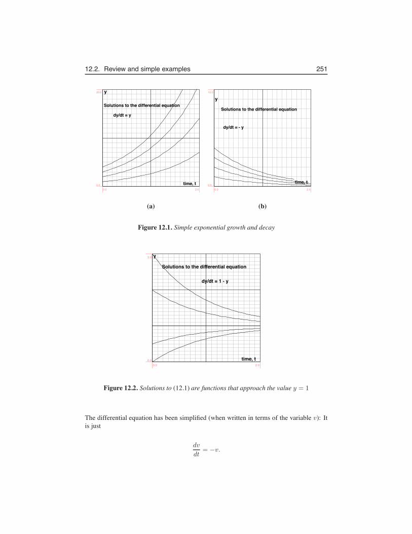
12.2. Review and simple examples 251
dy/dt = y
Solutions to the differential equation
y
time, t0.0 2.0
0.0
20.0
dy/dt = - y
Solutions to the differential equation
y
time, t0.0 2.0
0.0
10.0
(a) (b)
Figure 12.1. Simple exponential growth and decay
dy/dt = 1 - y
Solutions to the differential equation
time, t
y
0.0 2.00.0
3.0
Figure 12.2. Solutions to (12.1) are functions that approach the value y = 1
The differential equation has been simplified (when written in terms of the variable v): Itis just
dv
dt= −v.
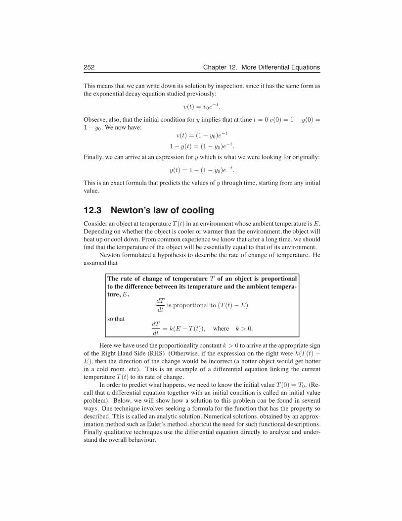
252 Chapter 12. More Differential Equations
This means that we can write down its solution by inspection, since it has the same form asthe exponential decay equation studied previously:
v(t) = v0e−t.
Observe, also, that the initial condition for y implies that at time t = 0 v(0) = 1− y(0) =1− y0. We now have:
v(t) = (1− y0)e−t
1− y(t) = (1 − y0)e−t.
Finally, we can arrive at an expression for y which is what we were looking for originally:
y(t) = 1− (1 − y0)e−t.
This is an exact formula that predicts the values of y through time, starting from any initialvalue.
12.3 Newton’s law of coolingConsider an object at temperature T (t) in an environment whose ambient temperature is E.Depending on whether the object is cooler or warmer than the environment, the object willheat up or cool down. From common experience we know that after a long time, we shouldfind that the temperature of the object will be essentially equal to that of its environment.
Newton formulated a hypothesis to describe the rate of change of temperature. Heassumed that
The rate of change of temperature T of an object is proportionalto the difference between its temperature and the ambient tempera-ture, E.
dT
dtis proportional to (T (t)− E)
so thatdT
dt= k(E − T (t)), where k > 0.
Here we have used the proportionality constant k > 0 to arrive at the appropriate signof the Right Hand Side (RHS). (Otherwise, if the expression on the right were k(T (t) −E), then the direction of the change would be incorrect (a hotter object would get hotterin a cold room, etc). This is an example of a differential equation linking the currenttemperature T (t) to its rate of change.
In order to predict what happens, we need to know the initial value T (0) = T0. (Re-call that a differential equation together with an initial condition is called an initial valueproblem). Below, we will show how a solution to this problem can be found in severalways. One technique involves seeking a formula for the function that has the property sodescribed. This is called an analytic solution. Numerical solutions, obtained by an approx-imation method such as Euler’s method, shortcut the need for such functional descriptions.Finally qualitative techniques use the differential equation directly to analyze and under-stand the overall behaviour.
12.3. Newton’s law of cooling 253
An analytic solution to Newton’s law of cooling
Considering the temperature T (t) as a function of time, we would like to solve the differ-ential equation
dT
dt= k(E − T ),
together with the initial conditionT (0) = T0.
We will assume that the ambient temperature, E is constant, as is the thermal con-ductivity, k > 0. We are hoping to identify a function T (t) that satisfies this equation, i.e.such that when we differentiate this function we find that
dT (t)
dt= k(E − T (t)).
The same “trick” as before can be used to convert this to an equation that we know how tosolve. If we define a new variable, v(t) = E − T (t), we can show that
dv(t)
dt= −kv
(This is left as an exercise for the reader.) We can also see that v(0) = E−T (0) = E−T0.Just as in the previous example, when the dust clears, we can find the formula for thesolution, which turns out to be
T (t) = E + (T0 − E)e−kt.
In Figure 12.3 we show a number of the curves that describe this behaviour for fivedifferent starting values of the temperature. (We have set E = 10 and k = 0.2 in this case.)This set of curves is often called the solution curves to the differential equation.
0
5
10
15
20temperature
0 5 10 15 20time
Figure 12.3. Temperature versus time for a cooling object
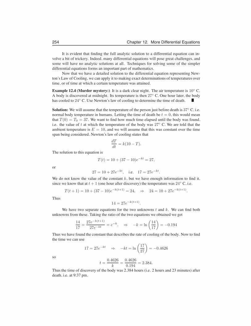
254 Chapter 12. More Differential Equations
It is evident that finding the full analytic solution to a differential equation can in-volve a bit of trickery. Indeed, many differential equations will pose great challenges, andsome will have no analytic solutions at all. Techniques for solving some of the simplerdifferential equations forms an important part of mathematics.
Now that we have a detailed solution to the differential equation representing New-ton’s Law of Cooling, we can apply it to making exact determinations of temperatures overtime, or of time at which a certain temperature was attained.
Example 12.4 (Murder mystery:) It is a dark clear night. The air temperature is 10◦ C.A body is discovered at midnight. Its temperature is then 27◦ C. One hour later, the bodyhas cooled to 24◦ C. Use Newton’s law of cooling to determine the time of death.
Solution: We will assume that the temperature of the person just before death is 37◦ C, i.e.normal body temperature in humans. Letting the time of death be t = 0, this would meanthat T (0) = T0 = 37. We want to find how much time elapsed until the body was found,i.e. the value of t at which the temperature of the body was 27◦ C. We are told that theambient temperature is E = 10, and we will assume that this was constant over the timespan being considered. Newton’s law of cooling states that
dT
dt= k(10− T ).
The solution to this equation is
T (t) = 10 + (37− 10)e−kt = 27,
or27 = 10 + 27e−kt, i.e. 17 = 27e−kt.
We do not know the value of the constant k, but we have enough information to find it,since we know that at t+ 1 (one hour after discovery) the temperature was 24◦ C, i.e.
T (t+ 1) = 10 + (37− 10)e−k(t+1) = 24, ⇒ 24 = 10 + 27e−k(t+1).
Thus14 = 27e−k(t+1).
We have two separate equations for the two unknowns t and k. We can find bothunknowns from these. Taking the ratio of the two equations we obtained we get
14
17=
27e−k(t+1)
27e−kt= e−k. ⇒ −k = ln
(
14
17
)
= −0.194
Thus we have found the constant that describes the rate of cooling of the body. Now to findthe time we can use
17 = 27e−kt ⇒ −kt = ln
(
17
27
)
= −0.4626
sot =
0.4626
k=
0.4626
0.194= 2.384.
Thus the time of discovery of the body was 2.384 hours (i.e. 2 hours and 23 minutes) afterdeath, i.e. at 9:37 pm.
12.4. Related examples 255
12.4 Related examplesThe differential equation that we have studied in Newton’s Law of Cooling is one repre-sentative member of a class of differential equations that share similar behaviour. In thissection we describe a more general form, comment on the general aspects of the solutionsand list a few other examples. Consider the differential equation
dy
dt= a− by
where a, b are constants together with the initial value
y(0) = y0.
While this appears to be an example unrelated to our previous work, by a slight reinterpre-tation, we will see the connection.
Rewrite the differential equation in the form
dy
dt= b
(a
b− y
)
Now note that our previous differential equation for cooling can be translated into the newequation by the following correspondence:
T (t) → y(t), E →a
b, k → b.
Rewriting Newton’s Law of Cooling in this notation produces the equation given above.But we are already familiar with all aspects of the solution to the previous problem ofcooling, so, just be reinterpreting it in terms of new quantities, we get the correspondingsolution to the more general differential equation:
y(t) =(
y0 −a
b
)
e−bt +a
b
Remarks made in our discussion of cooling should carry over directly to this functionand to the behaviour it describes. For example, we find that dy/dt = 0 for y = a/b. Wealso note that after a long time the value of y(t) should approach a/b.
12.4.1 Friction and terminal velocityThe velocity of a falling object changes due to the acceleration of gravity, but friction has aneffect of slowing down this acceleration. The differential equation satisfied by the velocityv(t) of the falling object is
dv
dt= g − kv
where g is acceleration due to gravity and k is a constant that represents the effect offriction.
256 Chapter 12. More Differential Equations
12.4.2 Production and removal of a substanceAn infusion containing a fixed concentration of substance is introduced into a fixed vol-ume. Inside the volume, a chemical reaction results in decay of the substance at a rateproportional to its concentration. Letting c(t) denote the time-dependent concentration ofthe substance, we would obtain a differential equation of the form
dc
dt= Kin − γc
where Kin represents the rate of input of substance and γ the decay rate.We can understand the behaviour of these systems by translating our notation from
the general to the specific forms given above. For example,
c(t) → y(t), Kin → a, γ → b.
Thus the behaviour found in the general case, can be interpreted in each of the specificsituations of interest.
12.5 Qualitative methodsFinding the formula that described temperature over time involved some convenient re-casting of the problem into familiar form. However, not all differential equations are aseasily solved analytically. Furthermore, even when we find the analytic solution, it is notalways easy to interpret, graph, or understand. This motivates a number of simpler qual-itative methods that lead us to an overall understanding of the behaviour directly frominformation contained in the differential equation, without the challenges of finding a fullfunctional form of the solution. We describe some of these methods below.
12.5.1 Rates of changeA differential equation
dy
dt= f(y)
encodes information about the rate of change dy/dt of the variable y, and how this rate ofchange is linked to the current value of y. It can be helpful to sketch the way that the rate ofchange depends on y, because certain interesting conclusions emerge from such diagrams.
Example 12.5 Consider the differential equation
dy
dt= y − y3. (12.2)
Then the rate of change is f(y) = y − y3 . (This is the function on the right hand sideof the differential equation.) Use this observation to determine values of y for which y isstatic (does not change).
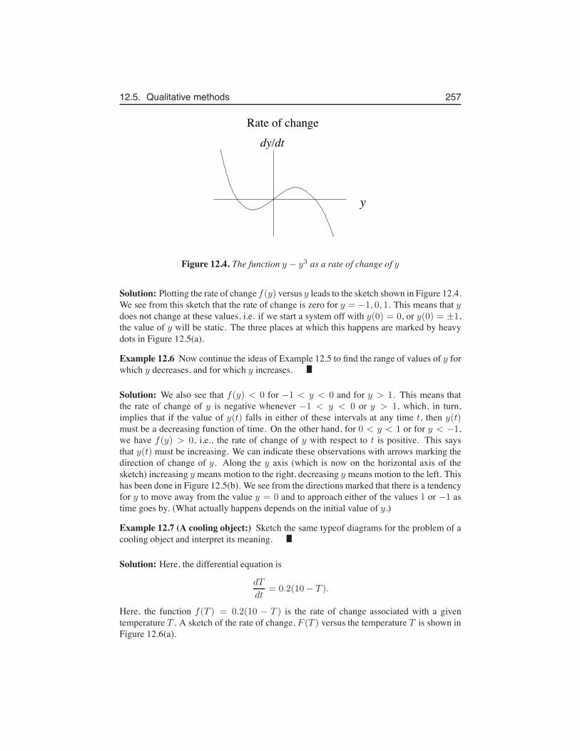
12.5. Qualitative methods 257
y
Rate of changedy/dt
Figure 12.4. The function y − y3 as a rate of change of y
Solution: Plotting the rate of change f(y) versus y leads to the sketch shown in Figure 12.4.We see from this sketch that the rate of change is zero for y = −1, 0, 1. This means that ydoes not change at these values, i.e. if we start a system off with y(0) = 0, or y(0) = ±1,the value of y will be static. The three places at which this happens are marked by heavydots in Figure 12.5(a).
Example 12.6 Now continue the ideas of Example 12.5 to find the range of values of y forwhich y decreases, and for which y increases.
Solution: We also see that f(y) < 0 for −1 < y < 0 and for y > 1. This means thatthe rate of change of y is negative whenever −1 < y < 0 or y > 1, which, in turn,implies that if the value of y(t) falls in either of these intervals at any time t, then y(t)must be a decreasing function of time. On the other hand, for 0 < y < 1 or for y < −1,we have f(y) > 0, i.e., the rate of change of y with respect to t is positive. This saysthat y(t) must be increasing. We can indicate these observations with arrows marking thedirection of change of y. Along the y axis (which is now on the horizontal axis of thesketch) increasing y means motion to the right, decreasing y means motion to the left. Thishas been done in Figure 12.5(b). We see from the directions marked that there is a tendencyfor y to move away from the value y = 0 and to approach either of the values 1 or −1 astime goes by. (What actually happens depends on the initial value of y.)
Example 12.7 (A cooling object:) Sketch the same typeof diagrams for the problem of acooling object and interpret its meaning.
Solution: Here, the differential equation is
dT
dt= 0.2(10− T ).
Here, the function f(T ) = 0.2(10 − T ) is the rate of change associated with a giventemperature T . A sketch of the rate of change, F (T ) versus the temperature T is shown inFigure 12.6(a).
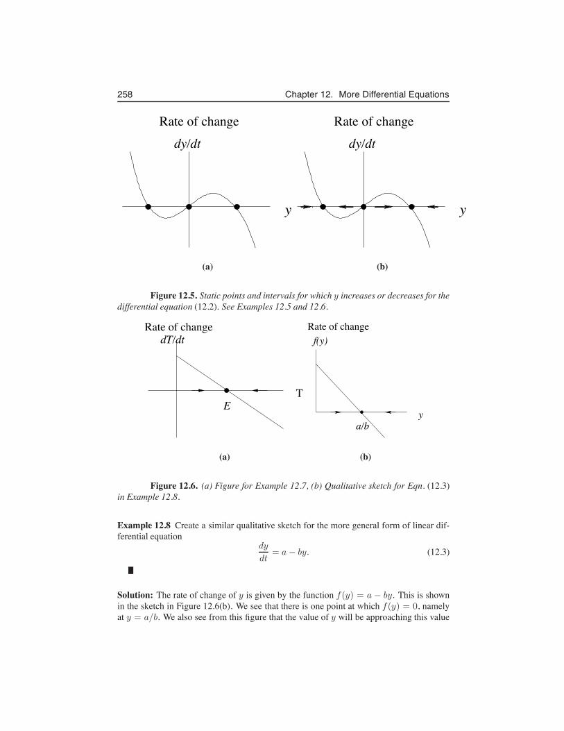
258 Chapter 12. More Differential Equations
y
Rate of changedy/dt
y
Rate of changedy/dt
(a) (b)
Figure 12.5. Static points and intervals for which y increases or decreases for thedifferential equation (12.2). See Examples 12.5 and 12.6.
Rate of change
T
dT/dt
E
f(y)
y
Rate of change
a/b
(a) (b)
Figure 12.6. (a) Figure for Example 12.7, (b) Qualitative sketch for Eqn. (12.3)in Example 12.8.
Example 12.8 Create a similar qualitative sketch for the more general form of linear dif-ferential equation
dy
dt= a− by. (12.3)
Solution: The rate of change of y is given by the function f(y) = a − by. This is shownin the sketch in Figure 12.6(b). We see that there is one point at which f(y) = 0, namelyat y = a/b. We also see from this figure that the value of y will be approaching this value
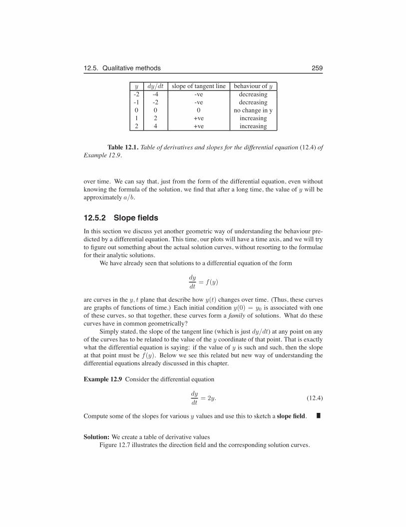
12.5. Qualitative methods 259
y dy/dt slope of tangent line behaviour of y-2 -4 -ve decreasing-1 -2 -ve decreasing0 0 0 no change in y1 2 +ve increasing2 4 +ve increasing
Table 12.1. Table of derivatives and slopes for the differential equation (12.4) ofExample 12.9.
over time. We can say that, just from the form of the differential equation, even withoutknowing the formula of the solution, we find that after a long time, the value of y will beapproximately a/b.
12.5.2 Slope fieldsIn this section we discuss yet another geometric way of understanding the behaviour pre-dicted by a differential equation. This time, our plots will have a time axis, and we will tryto figure out something about the actual solution curves, without resorting to the formulaefor their analytic solutions.
We have already seen that solutions to a differential equation of the form
dy
dt= f(y)
are curves in the y, t plane that describe how y(t) changes over time. (Thus, these curvesare graphs of functions of time.) Each initial condition y(0) = y0 is associated with oneof these curves, so that together, these curves form a family of solutions. What do thesecurves have in common geometrically?
Simply stated, the slope of the tangent line (which is just dy/dt) at any point on anyof the curves has to be related to the value of the y coordinate of that point. That is exactlywhat the differential equation is saying: if the value of y is such and such, then the slopeat that point must be f(y). Below we see this related but new way of understanding thedifferential equations already discussed in this chapter.
Example 12.9 Consider the differential equation
dy
dt= 2y. (12.4)
Compute some of the slopes for various y values and use this to sketch a slope field.
Solution: We create a table of derivative valuesFigure 12.7 illustrates the direction field and the corresponding solution curves.
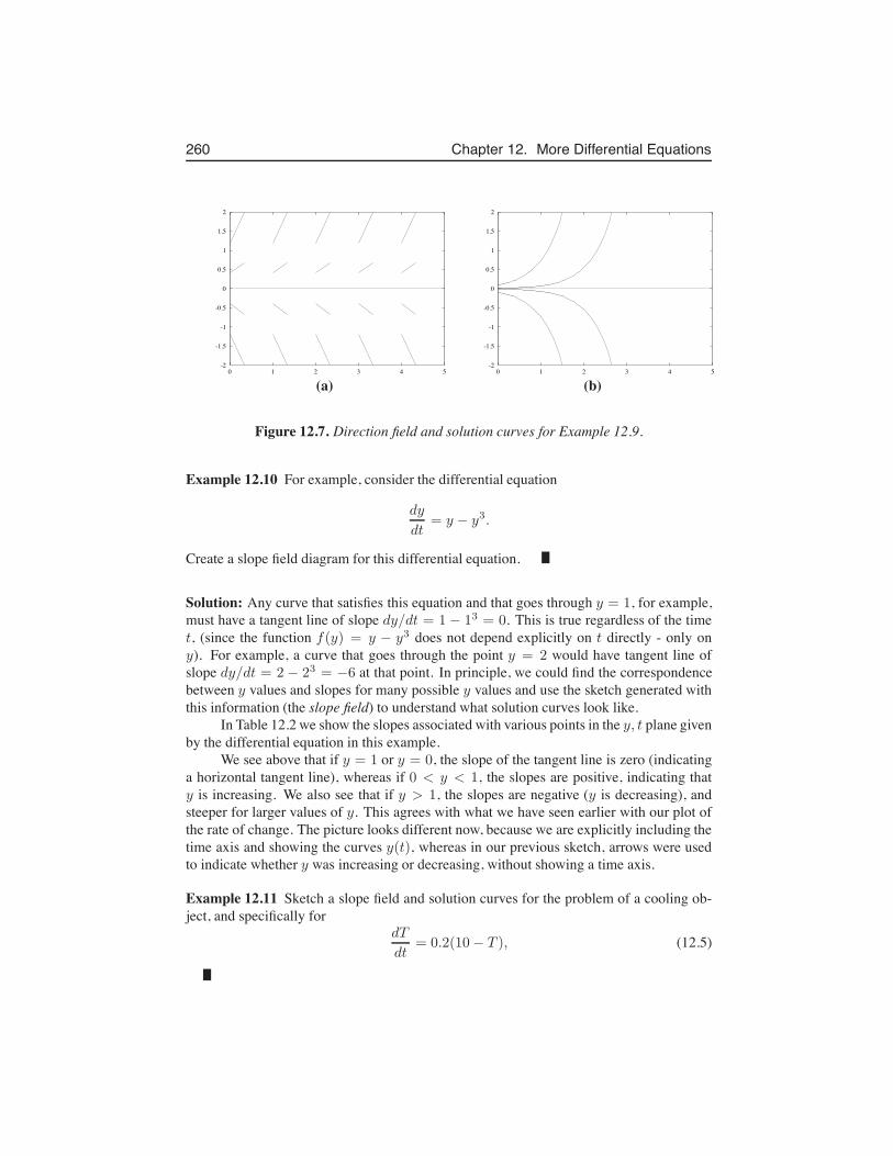
260 Chapter 12. More Differential Equations
-2
-1.5
-1
-0.5
0
0.5
1
1.5
2
0 1 2 3 4 5-2
-1.5
-1
-0.5
0
0.5
1
1.5
2
0 1 2 3 4 5
(a) (b)
Figure 12.7. Direction field and solution curves for Example 12.9.
Example 12.10 For example, consider the differential equation
dy
dt= y − y3.
Create a slope field diagram for this differential equation.
Solution: Any curve that satisfies this equation and that goes through y = 1, for example,must have a tangent line of slope dy/dt = 1 − 13 = 0. This is true regardless of the timet, (since the function f(y) = y − y3 does not depend explicitly on t directly - only ony). For example, a curve that goes through the point y = 2 would have tangent line ofslope dy/dt = 2 − 23 = −6 at that point. In principle, we could find the correspondencebetween y values and slopes for many possible y values and use the sketch generated withthis information (the slope field) to understand what solution curves look like.
In Table 12.2 we show the slopes associated with various points in the y, t plane givenby the differential equation in this example.
We see above that if y = 1 or y = 0, the slope of the tangent line is zero (indicatinga horizontal tangent line), whereas if 0 < y < 1, the slopes are positive, indicating thaty is increasing. We also see that if y > 1, the slopes are negative (y is decreasing), andsteeper for larger values of y. This agrees with what we have seen earlier with our plot ofthe rate of change. The picture looks different now, because we are explicitly including thetime axis and showing the curves y(t), whereas in our previous sketch, arrows were usedto indicate whether y was increasing or decreasing, without showing a time axis.
Example 12.11 Sketch a slope field and solution curves for the problem of a cooling ob-ject, and specifically for
dT
dt= 0.2(10− T ), (12.5)
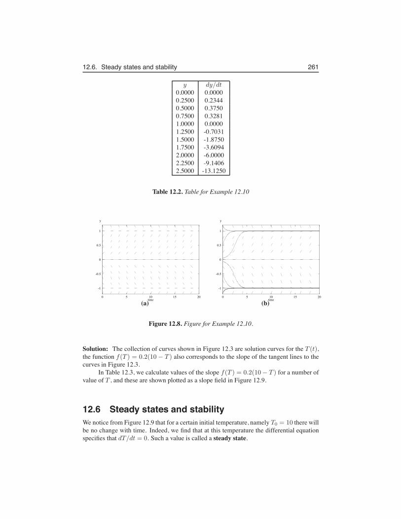
12.6. Steady states and stability 261
y dy/dt0.0000 0.00000.2500 0.23440.5000 0.37500.7500 0.32811.0000 0.00001.2500 -0.70311.5000 -1.87501.7500 -3.60942.0000 -6.00002.2500 -9.14062.5000 -13.1250
Table 12.2. Table for Example 12.10
-1
-0.5
0
0.5
1
y
0 5 10 15 20time
-1
-0.5
0
0.5
1
y
0 5 10 15 20time(a) (b)
Figure 12.8. Figure for Example 12.10.
Solution: The collection of curves shown in Figure 12.3 are solution curves for the T (t),the function f(T ) = 0.2(10 − T ) also corresponds to the slope of the tangent lines to thecurves in Figure 12.3.
In Table 12.3, we calculate values of the slope f(T ) = 0.2(10− T ) for a number ofvalue of T , and these are shown plotted as a slope field in Figure 12.9.
12.6 Steady states and stabilityWe notice from Figure 12.9 that for a certain initial temperature, namely T0 = 10 there willbe no change with time. Indeed, we find that at this temperature the differential equationspecifies that dT/dt = 0. Such a value is called a steady state.
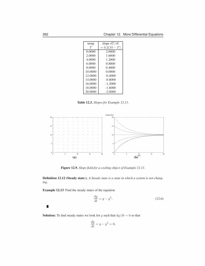
262 Chapter 12. More Differential Equations
temp slope dT/dtT = 0.2(10− T )
0.0000 2.00002.0000 1.60004.0000 1.20006.0000 0.80008.0000 0.4000
10.0000 0.000012.0000 -0.400014.0000 -0.800016.0000 -1.200018.0000 -1.600020.0000 -2.0000
Table 12.3. Slopes for Example 12.11.
0
5
10
15
20
0 5 10 15 200
5
10
15
20temperature
0 5 10 15 20time(a) (b)
Figure 12.9. Slope field for a cooling object of Example 12.11.
Definition 12.12 (Steady state:). A Steady state is a state in which a system is not chang-ing.
Example 12.13 Find the steady states of the equation
dy
dt= y − y3, (12.6)
Solution: To find steady states we look for y such that dy/dt = 0 so that
dy
dt= y − y3 = 0,
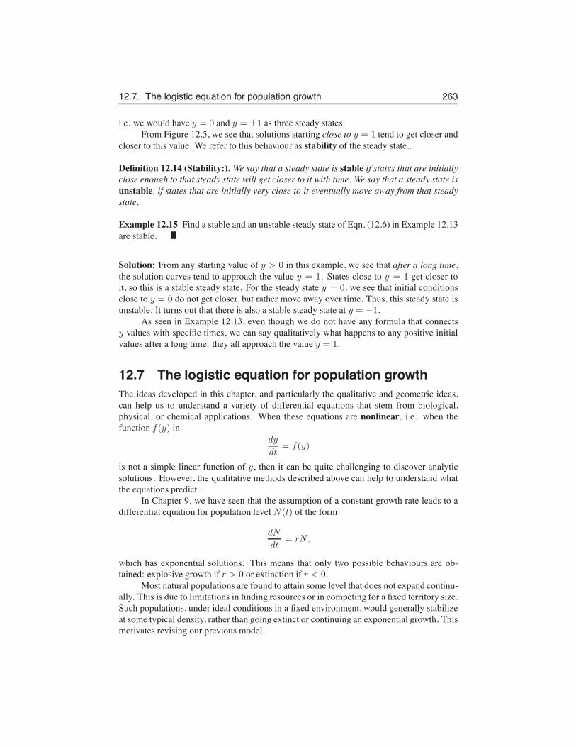
12.7. The logistic equation for population growth 263
i.e. we would have y = 0 and y = ±1 as three steady states.From Figure 12.5, we see that solutions starting close to y = 1 tend to get closer and
closer to this value. We refer to this behaviour as stability of the steady state..
Definition 12.14 (Stability:). We say that a steady state is stable if states that are initiallyclose enough to that steady state will get closer to it with time. We say that a steady state isunstable, if states that are initially very close to it eventually move away from that steadystate.
Example 12.15 Find a stable and an unstable steady state of Eqn. (12.6) in Example 12.13are stable.
Solution: From any starting value of y > 0 in this example, we see that after a long time,the solution curves tend to approach the value y = 1. States close to y = 1 get closer toit, so this is a stable steady state. For the steady state y = 0, we see that initial conditionsclose to y = 0 do not get closer, but rather move away over time. Thus, this steady state isunstable. It turns out that there is also a stable steady state at y = −1.
As seen in Example 12.13, even though we do not have any formula that connectsy values with specific times, we can say qualitatively what happens to any positive initialvalues after a long time: they all approach the value y = 1.
12.7 The logistic equation for population growthThe ideas developed in this chapter, and particularly the qualitative and geometric ideas,can help us to understand a variety of differential equations that stem from biological,physical, or chemical applications. When these equations are nonlinear, i.e. when thefunction f(y) in
dy
dt= f(y)
is not a simple linear function of y, then it can be quite challenging to discover analyticsolutions. However, the qualitative methods described above can help to understand whatthe equations predict.
In Chapter 9, we have seen that the assumption of a constant growth rate leads to adifferential equation for population level N(t) of the form
dN
dt= rN,
which has exponential solutions. This means that only two possible behaviours are ob-tained: explosive growth if r > 0 or extinction if r < 0.
Most natural populations are found to attain some level that does not expand continu-ally. This is due to limitations in finding resources or in competing for a fixed territory size.Such populations, under ideal conditions in a fixed environment, would generally stabilizeat some typical density, rather than going extinct or continuing an exponential growth. Thismotivates revising our previous model.
264 Chapter 12. More Differential Equations
In the modification studied here, we will let N(t) represent the size of a populationat time t. Consider the differential equation
dN
dt= rN
(K −N)
K. (12.7)
We call this the differential equation the logistic equation. Here the parameter r > 0is called the intrinsic growth rate and K > 0 is the carrying capacity. Both theseparameters are assumed to be positive constants.
The logistic equation can be justified in one of several ways as a convenient simplemodel for population growth that has a greater relevance than exponential growth. In theform written above, we could interpret it at
dN
dt= R(N)N.
where R(N) = r(K −N)/K is a so-called density dependent growth rate. (It replacesthe previously assumed constant growth rate rN , that leads to unlimited growth.) Rewrittenin the form
dN
dt= rN − bN2
(where b = r/K is a positive quantity), it can be interpreted as the usual linear growthterm rN , with a superimposed quadratic (nonlinear) rate of death due to overcrowding orcompetition bN2. We already know that this quadratic term will dominate for larger valuesof N , and this means that when the population is crowded, the loss of individuals is greaterthan the rate of reproduction.
In this section we will familiarize ourselves with the behaviour predicted by the lo-gistic equation.
Example 12.16 Find the steady states of the Logistic Equation (12.7).
Solution: To determine the steady states of the equation (12.7), i.e. the level of populationthat would not change over time, we look for values of N such that
dN
dt= 0
This leads torN
(K −N)
K= 0
which has solutions N = 0 (no population at all) or N = K (the population is at itscarrying capacity).
The logistic equation has a long history in modelling population growth of microor-ganisms, animals, and human populations. It is justified either by considering it to be aspecial case of the density dependent growth equation
dN
dt= R(N)N
12.7. The logistic equation for population growth 265
(In that case the reproductive rate has the form R(N) = r(K −N)/K), or, equivalently, itcan be considered to fall into a class of equations that have the form
dN
dt= rN − bN2
(where the constant is b = r/K), which means that a constant rate of reproduction rN ismodified by a quadratic mortality rate bN2. The mortality would tend to dominate onlyfor larger values of the population, i.e. if conditions are crowded so that animals haveto compete for resources or habitat. (This stems from the fact that the quadratic term issmaller than the linear term near N = 0, but dominates for large N , as we have alreadydiscussed in Chapter 1.)
It is often desirable to formulate the problem in the simplest possible terms. We cando this by a process called rescaling:
Example 12.17 (Rescaling:) Define a new variable
y(t) =N(t)
K.
Interpret what this variable represents and show that the Logistic equation can be writtenin a simpler form in terms of this variable.
Solution: The rescaled variable, y(t), is a population density expressed in units of thecarrying capacity. (For example, if the environment can sustain 1000 individuals, and thecurrent population size is N = 950 then the value of y is y = 0.950.) Since K is assumedconstant,
dy
dt=
1
K
dN
dt
and we can simplify the equation:
dy
dt= ry(1 − y). (12.8)
We observe that indeed, this equation “looks simpler” and also has only one constant pa-rameter left in it. It is generally the case that rescaling reduces the number of parameters ina differential equation such as seen here.
Example 12.18 Draw a plot of the rate of change dy/dt versus the value of y for therescaled logistic equation (12.8).
Solution: This plot is shown in Figure 12.10. The steady states are located at y = 0, 1(which correspond to N = 0 and N = K in the original variable.) We also find that in theinterval 0 < y < 1, the rate of change is positive, so that y increases, whereas for y > 1,the rate of change is negative, so y decreases. Since y refers to population size, we neednot concern ourselves with behaviour for y < 0.
From Figure 12.10 we expect to see solutions to the differential equation that ap-proach the value y = 1 after a long time. (The only exception to this would be the case
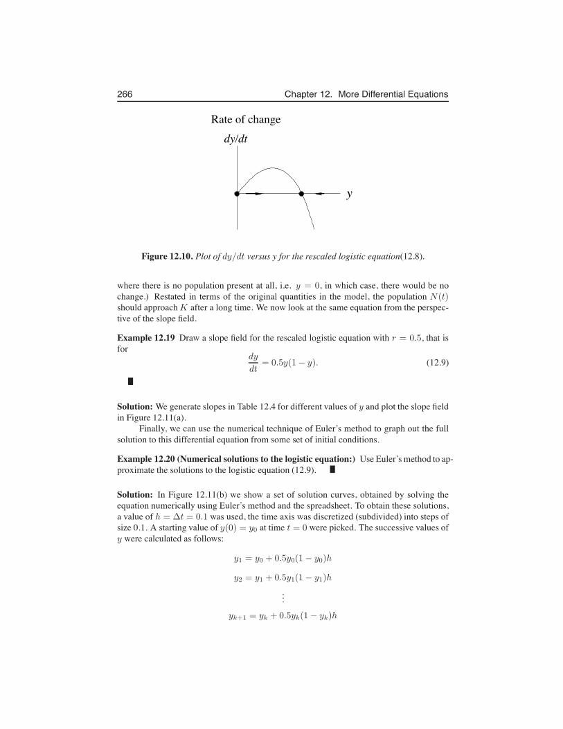
266 Chapter 12. More Differential Equations
Rate of changedy/dt
y
Figure 12.10. Plot of dy/dt versus y for the rescaled logistic equation(12.8).
where there is no population present at all, i.e. y = 0, in which case, there would be nochange.) Restated in terms of the original quantities in the model, the population N(t)should approach K after a long time. We now look at the same equation from the perspec-tive of the slope field.
Example 12.19 Draw a slope field for the rescaled logistic equation with r = 0.5, that isfor
dy
dt= 0.5y(1− y). (12.9)
Solution: We generate slopes in Table 12.4 for different values of y and plot the slope fieldin Figure 12.11(a).
Finally, we can use the numerical technique of Euler’s method to graph out the fullsolution to this differential equation from some set of initial conditions.
Example 12.20 (Numerical solutions to the logistic equation:) Use Euler’s method to ap-proximate the solutions to the logistic equation (12.9).
Solution: In Figure 12.11(b) we show a set of solution curves, obtained by solving theequation numerically using Euler’s method and the spreadsheet. To obtain these solutions,a value of h = ∆t = 0.1 was used, the time axis was discretized (subdivided) into steps ofsize 0.1. A starting value of y(0) = y0 at time t = 0 were picked. The successive values ofy were calculated as follows:
y1 = y0 + 0.5y0(1− y0)h
y2 = y1 + 0.5y1(1− y1)h
...
yk+1 = yk + 0.5yk(1− yk)h
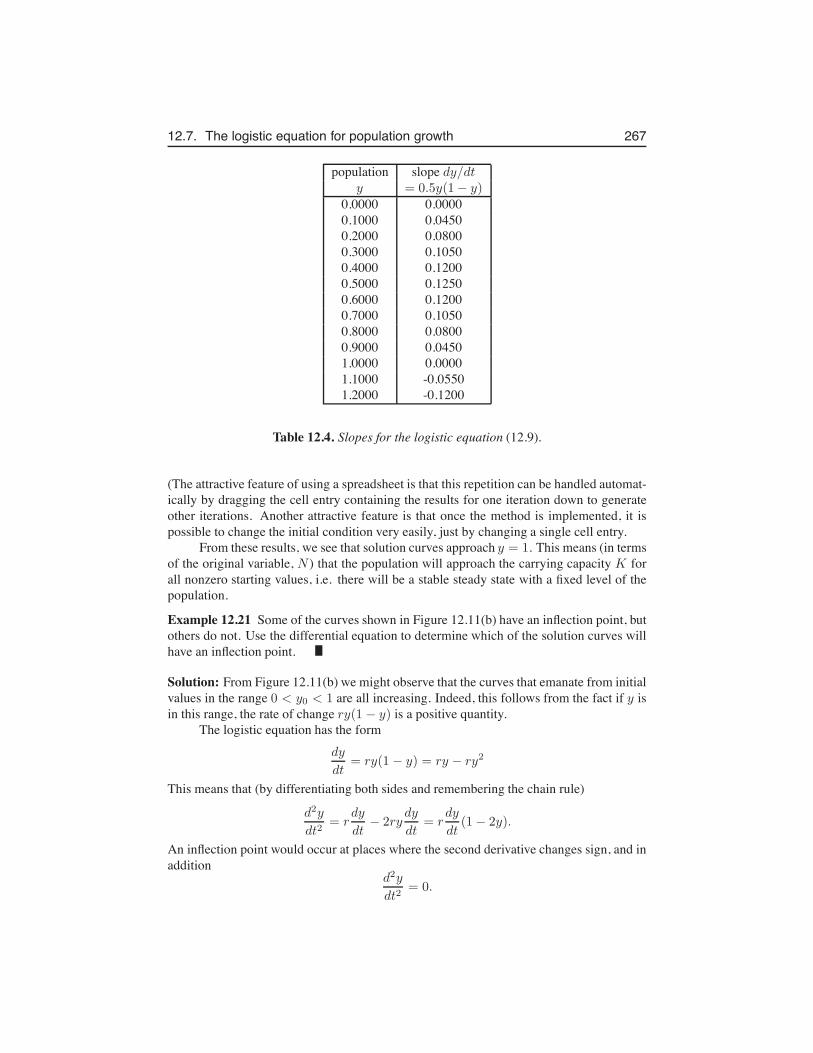
12.7. The logistic equation for population growth 267
population slope dy/dty = 0.5y(1− y)
0.0000 0.00000.1000 0.04500.2000 0.08000.3000 0.10500.4000 0.12000.5000 0.12500.6000 0.12000.7000 0.10500.8000 0.08000.9000 0.04501.0000 0.00001.1000 -0.05501.2000 -0.1200
Table 12.4. Slopes for the logistic equation (12.9).
(The attractive feature of using a spreadsheet is that this repetition can be handled automat-ically by dragging the cell entry containing the results for one iteration down to generateother iterations. Another attractive feature is that once the method is implemented, it ispossible to change the initial condition very easily, just by changing a single cell entry.
From these results, we see that solution curves approach y = 1. This means (in termsof the original variable, N ) that the population will approach the carrying capacity K forall nonzero starting values, i.e. there will be a stable steady state with a fixed level of thepopulation.
Example 12.21 Some of the curves shown in Figure 12.11(b) have an inflection point, butothers do not. Use the differential equation to determine which of the solution curves willhave an inflection point.
Solution: From Figure 12.11(b) we might observe that the curves that emanate from initialvalues in the range 0 < y0 < 1 are all increasing. Indeed, this follows from the fact if y isin this range, the rate of change ry(1 − y) is a positive quantity.
The logistic equation has the formdy
dt= ry(1 − y) = ry − ry2
This means that (by differentiating both sides and remembering the chain rule)
d2y
dt2= r
dy
dt− 2ry
dy
dt= r
dy
dt(1− 2y).
An inflection point would occur at places where the second derivative changes sign, and inaddition
d2y
dt2= 0.
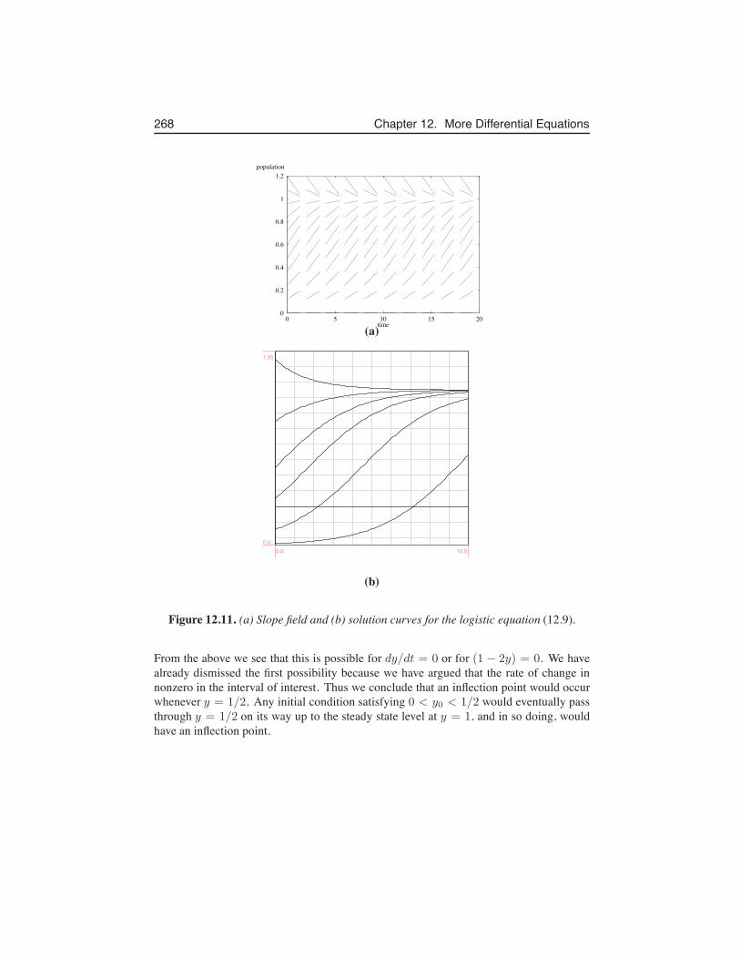
268 Chapter 12. More Differential Equations
0
0.2
0.4
0.6
0.8
1
1.2population
0 5 10 15 20time(a)
0.0 10.00.0
1.25
(b)
Figure 12.11. (a) Slope field and (b) solution curves for the logistic equation (12.9).
From the above we see that this is possible for dy/dt = 0 or for (1 − 2y) = 0. We havealready dismissed the first possibility because we have argued that the rate of change innonzero in the interval of interest. Thus we conclude that an inflection point would occurwhenever y = 1/2. Any initial condition satisfying 0 < y0 < 1/2 would eventually passthrough y = 1/2 on its way up to the steady state level at y = 1, and in so doing, wouldhave an inflection point.
Exercises 269
Exercises12.1. Consider the differential equation
dy
dt= a− by
where a, b are constants.(a) Show that the function
y(t) =a
b− Ce−bt
satisfies the above differential equation for any constant C.(b) Show that by setting
C =a
b− y0
we also satisfy the initial condition
y(0) = y0.
Remark: You have now shown that the function
y(t) =(
y0 −a
b
)
e−bt +a
b
is a solution to the initial value problem (i.e differential equation plus initialcondition)
dy
dt= a− by, y(0) = y0.
12.2. For each of the following, show the given function y is a solution to the given dif-ferential equation.
(a) t ·dy
dt= 3y, y = 2t3.
(b)d2y
dt2+ y = 0, y = −2 sin t+ 3 cos t.
(c) d2y
dt2− 2
dy
dt+ y = 6et, y = 3t2et.
12.3. Show the function determined by the equation 2x2 + xy − y2 = C, where C is aconstant and 2y $= x, is a solution to the differential equation (x−2y)
dy
dx= −4x−y.
12.4. Find the constant C that satisfies the given initial conditions.(a) 2x2 − 3y2 = C, y|x=0 = 2.(b) y = C1e5t + C2te5t, y|t=0 = 1 and dy
dt |t=0 = 0.
(c) y = C1 cos(t− C2), y|t=π2= 0 and dy
dt |t=π2= 1.
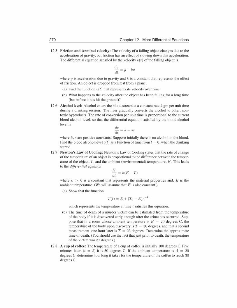
270 Chapter 12. More Differential Equations
12.5. Friction and terminal velocity: The velocity of a falling object changes due to theacceleration of gravity, but friction has an effect of slowing down this acceleration.The differential equation satisfied by the velocity v(t) of the falling object is
dv
dt= g − kv
where g is acceleration due to gravity and k is a constant that represents the effectof friction. An object is dropped from rest from a plane.
(a) Find the function v(t) that represents its velocity over time.(b) What happens to the velocity after the object has been falling for a long time
(but before it has hit the ground)?12.6. Alcohol level: Alcohol enters the blood stream at a constant rate k gm per unit time
during a drinking session. The liver gradually converts the alcohol to other, non-toxic byproducts. The rate of conversion per unit time is proportional to the currentblood alcohol level, so that the differential equation satisfied by the blood alcohollevel is
dc
dt= k − sc
where k, s are positive constants. Suppose initially there is no alcohol in the blood.Find the blood alcohol level c(t) as a function of time from t = 0, when the drinkingstarted.
12.7. Newton’s Law of Cooling: Newton’s Law of Cooling states that the rate of changeof the temperature of an object is proportional to the difference between the temper-ature of the object, T , and the ambient (environmental) temperature, E. This leadsto the differential equation
dT
dt= k(E − T )
where k > 0 is a constant that represents the material properties and, E is theambient temperature. (We will assume that E is also constant.)
(a) Show that the function
T (t) = E + (T0 − E)e−kt
which represents the temperature at time t satisfies this equation.(b) The time of death of a murder victim can be estimated from the temperature
of the body if it is discovered early enough after the crime has occurred. Sup-pose that in a room whose ambient temperature is E = 20 degrees C, thetemperature of the body upon discovery is T = 30 degrees, and that a secondmeasurement, one hour later is T = 25 degrees. Determine the approximatetime of death. (You should use the fact that just prior to death, the temperatureof the victim was 37 degrees.)
12.8. A cup of coffee: The temperature of a cup of coffee is initially 100 degrees C. Fiveminutes later, (t = 5) it is 50 degrees C. If the ambient temperature is A = 20degrees C, determine how long it takes for the temperature of the coffee to reach 30degrees C.
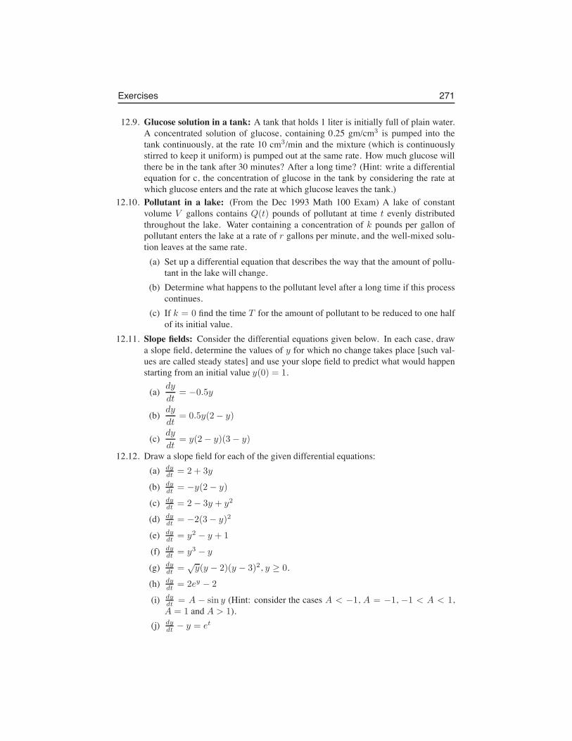
Exercises 271
12.9. Glucose solution in a tank: A tank that holds 1 liter is initially full of plain water.A concentrated solution of glucose, containing 0.25 gm/cm3 is pumped into thetank continuously, at the rate 10 cm3/min and the mixture (which is continuouslystirred to keep it uniform) is pumped out at the same rate. How much glucose willthere be in the tank after 30 minutes? After a long time? (Hint: write a differentialequation for c, the concentration of glucose in the tank by considering the rate atwhich glucose enters and the rate at which glucose leaves the tank.)
12.10. Pollutant in a lake: (From the Dec 1993 Math 100 Exam) A lake of constantvolume V gallons contains Q(t) pounds of pollutant at time t evenly distributedthroughout the lake. Water containing a concentration of k pounds per gallon ofpollutant enters the lake at a rate of r gallons per minute, and the well-mixed solu-tion leaves at the same rate.
(a) Set up a differential equation that describes the way that the amount of pollu-tant in the lake will change.
(b) Determine what happens to the pollutant level after a long time if this processcontinues.
(c) If k = 0 find the time T for the amount of pollutant to be reduced to one halfof its initial value.
12.11. Slope fields: Consider the differential equations given below. In each case, drawa slope field, determine the values of y for which no change takes place [such val-ues are called steady states] and use your slope field to predict what would happenstarting from an initial value y(0) = 1.
(a) dy
dt= −0.5y
(b) dy
dt= 0.5y(2− y)
(c) dy
dt= y(2− y)(3− y)
12.12. Draw a slope field for each of the given differential equations:(a) dy
dt = 2 + 3y
(b) dydt = −y(2− y)
(c) dydt = 2− 3y + y2
(d) dydt = −2(3− y)2
(e) dydt = y2 − y + 1
(f) dydt = y3 − y
(g) dydt =
√y(y − 2)(y − 3)2, y ≥ 0.
(h) dydt = 2ey − 2
(i) dydt = A − sin y (Hint: consider the cases A < −1, A = −1, −1 < A < 1,A = 1 and A > 1).
(j) dydt − y = et
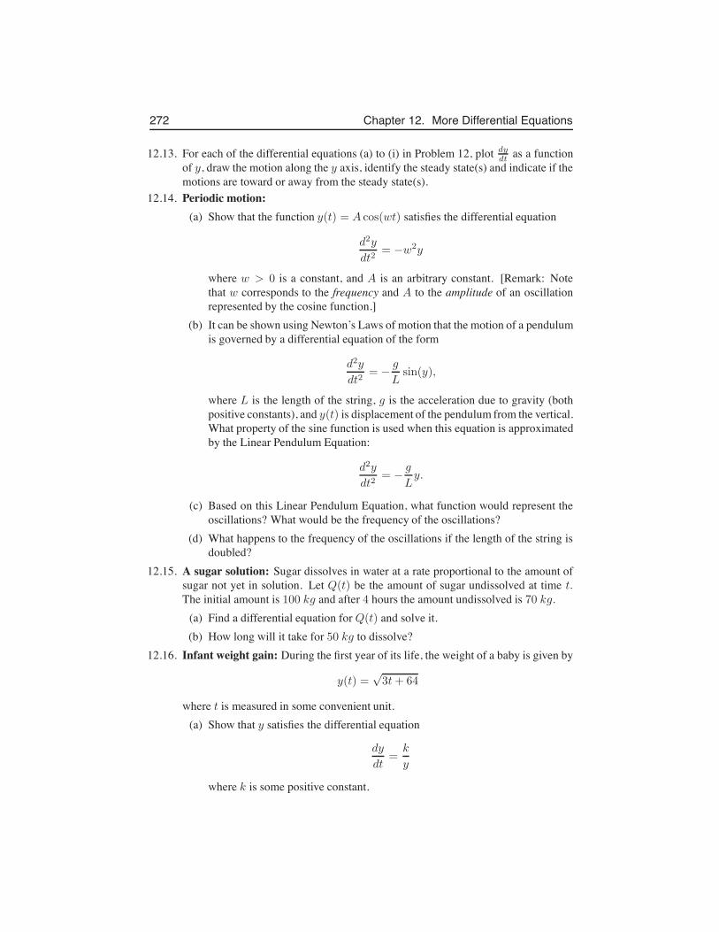
272 Chapter 12. More Differential Equations
12.13. For each of the differential equations (a) to (i) in Problem 12, plot dydt as a function
of y, draw the motion along the y axis, identify the steady state(s) and indicate if themotions are toward or away from the steady state(s).
12.14. Periodic motion:(a) Show that the function y(t) = A cos(wt) satisfies the differential equation
d2y
dt2= −w2y
where w > 0 is a constant, and A is an arbitrary constant. [Remark: Notethat w corresponds to the frequency and A to the amplitude of an oscillationrepresented by the cosine function.]
(b) It can be shown using Newton’s Laws of motion that the motion of a pendulumis governed by a differential equation of the form
d2y
dt2= −
g
Lsin(y),
where L is the length of the string, g is the acceleration due to gravity (bothpositive constants), and y(t) is displacement of the pendulum from the vertical.What property of the sine function is used when this equation is approximatedby the Linear Pendulum Equation:
d2y
dt2= −
g
Ly.
(c) Based on this Linear Pendulum Equation, what function would represent theoscillations? What would be the frequency of the oscillations?
(d) What happens to the frequency of the oscillations if the length of the string isdoubled?
12.15. A sugar solution: Sugar dissolves in water at a rate proportional to the amount ofsugar not yet in solution. Let Q(t) be the amount of sugar undissolved at time t.The initial amount is 100 kg and after 4 hours the amount undissolved is 70 kg.
(a) Find a differential equation for Q(t) and solve it.(b) How long will it take for 50 kg to dissolve?
12.16. Infant weight gain: During the first year of its life, the weight of a baby is given by
y(t) =√3t+ 64
where t is measured in some convenient unit.(a) Show that y satisfies the differential equation
dy
dt=
k
y
where k is some positive constant.
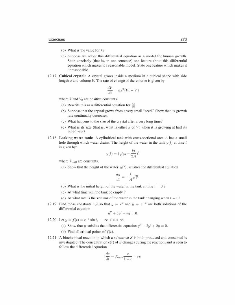
Exercises 273
(b) What is the value for k?(c) Suppose we adopt this differential equation as a model for human growth.
State concisely (that is, in one sentence) one feature about this differentialequation which makes it a reasonable model. State one feature which makes itunreasonable.
12.17. Cubical crystal: A crystal grows inside a medium in a cubical shape with sidelength x and volume V. The rate of change of the volume is given by
dV
dt= kx2(V0 − V )
where k and V0 are positive constants.(a) Rewrite this as a differential equation for dx
dt .
(b) Suppose that the crystal grows from a very small “seed.” Show that its growthrate continually decreases.
(c) What happens to the size of the crystal after a very long time?(d) What is its size (that is, what is either x or V ) when it is growing at half its
initial rate?12.18. Leaking water tank: A cylindrical tank with cross-sectional area A has a small
hole through which water drains. The height of the water in the tank y(t) at time tis given by:
y(t) = (√y0 −
kt
2A)2
where k, y0 are constants.(a) Show that the height of the water, y(t), satisfies the differential equation
dy
dt= −
k
A
√y.
(b) What is the initial height of the water in the tank at time t = 0 ?(c) At what time will the tank be empty ?(d) At what rate is the volume of the water in the tank changing when t = 0?
12.19. Find those constants a, b so that y = ex and y = e−x are both solutions of thedifferential equation
y′′ + ay′ + by = 0.
12.20. Let y = f(t) = e−t sin t, −∞ < t < ∞.
(a) Show that y satisfies the differential equation y′′ + 2y′ + 2y = 0.
(b) Find all critical points of f(t).12.21. A biochemical reaction in which a substance S is both produced and consumed is
investigated. The concentration c(t) of S changes during the reaction, and is seen tofollow the differential equation
dc
dt= Kmax
c
k + c− rc
274 Chapter 12. More Differential Equations
where Kmax, k, r are positive constants with certain convenient units. The first termis a concentration-dependent production term and the second term represents con-sumption of the substance.
(a) What is the maximal rate at which the substance is produced? At what con-centration is the production rate 50% of this maximal value?
(b) If the production is turned off, the substance will decay. How long would ittake for the concentration to drop by 50%?
(c)At what concentration does the production rate just balance the consumption rate?
Appendices
275

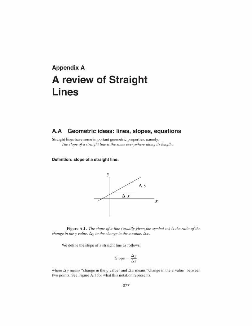
Appendix A
A review of StraightLines
A.A Geometric ideas: lines, slopes, equationsStraight lines have some important geometric properties, namely:
The slope of a straight line is the same everywhere along its length.
Definition: slope of a straight line:
' y
x
y
' x
Figure A.1. The slope of a line (usually given the symbol m) is the ratio of thechange in the y value, ∆y to the change in the x value, ∆x.
We define the slope of a straight line as follows:
Slope =∆y
∆x
where ∆y means “change in the y value” and ∆x means “change in the x value” betweentwo points. See Figure A.1 for what this notation represents.
277
278 Appendix A. A review of Straight Lines
Equation of a straight line
Using this basic geometric property, we can find the equation of a straight line given any ofthe following information about the line:
• The y intercept, b, and the slope, m:
y = mx+ b.
• A point (x0, y0) on the line, and the slope, m, of the line:
y − y0x− x0
= m
• Two points on the line, say (x1, y1) and (x2, y2):
y − y1x− x1
=y2 − y1x2 − x1
Remark: any of these can be rearranged or simplified to produce the standard formy = mx+ b, as discussed in the problem set.
The following examples will refresh your memory on how to find the equation of theline that satisfies each of the given conditions.
Example A.1 In each case write down the equation of the straight line that satisfies thegiven statements. (Note: you should also be able to easily sketch the line in each case.)
(a) The line has slope 2 and y intercept 4.
(b) The line goes through the points (1,1) and (3,-2).
(c) The line has y intercept -1 and x intercept 3.
(d) The line has slope -1 and goes through the point (-2,-5).
Solution:
(a) We can use the standard form of the equation of a straight line, y = mx + b wherem is the slope and b is the y intercept to obtain the equation: y = 2x+ 4
(b) The line goes through the points (1,1) and (3,-2). We use the fact that the slope is thesame all along the line. Thus,
(y − y0)
(x− x0)=
(y1 − y0)
(x1 − x0)= m.
Substituting in the values (x0, y0) = (1, 1) and (x1, y1) = (3,−2),
(y − 1)
(x− 1)=
(1 + 2)
(1− 3)= −
3
2.
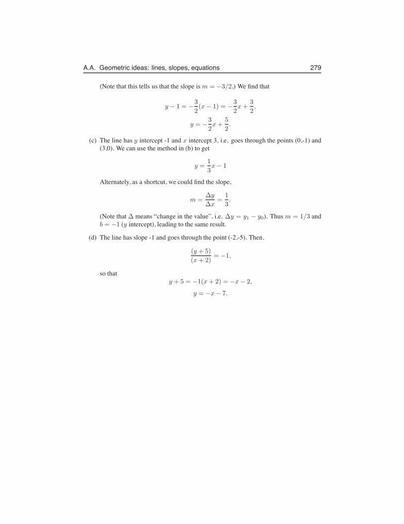
A.A. Geometric ideas: lines, slopes, equations 279
(Note that this tells us that the slope is m = −3/2.) We find that
y − 1 = −3
2(x− 1) = −
3
2x+
3
2,
y = −3
2x+
5
2.
(c) The line has y intercept -1 and x intercept 3, i.e. goes through the points (0,-1) and(3,0). We can use the method in (b) to get
y =1
3x− 1
Alternately, as a shortcut, we could find the slope,
m =∆y
∆x=
1
3.
(Note that ∆ means “change in the value”, i.e. ∆y = y1 − y0). Thus m = 1/3 andb = −1 (y intercept), leading to the same result.
(d) The line has slope -1 and goes through the point (-2,-5). Then,
(y + 5)
(x + 2)= −1,
so thaty + 5 = −1(x+ 2) = −x− 2,
y = −x− 7.
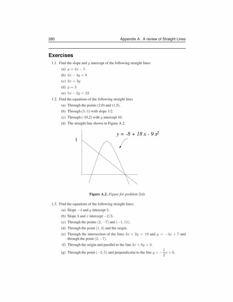
280 Appendix A. A review of Straight Lines
Exercises1.1. Find the slope and y intercept of the following straight lines:
(a) y = 4x− 5
(b) 3x− 4y = 8
(c) 2x = 3y
(d) y = 3
(e) 5x− 2y = 23
1.2. Find the equations of the following straight lines(a) Through the points (2,0) and (1,5).(b) Through (3,-1) with slope 1/2.(c) Through (-10,2) with y intercept 10.(d) The straight line shown in Figure A.2.
1y = -8 + 18 x - 9 x 2
Figure A.2. Figure for problem 2(d)
1.3. Find the equations of the following straight lines:(a) Slope −4 and y intercept 3.(b) Slope 3 and x intercept −2/3.(c) Through the points (2,−7) and (−1, 11).(d) Through the point (1, 3) and the origin.(e) Through the intersection of the lines 3x + 2y = 19 and y = −4x + 7 and
through the point (2,−7).(f) Through the origin and parallel to the line 2x+ 8y = 3.
(g) Through the point (−2, 5) and perpendicular to the line y = −1
2x+ 6.
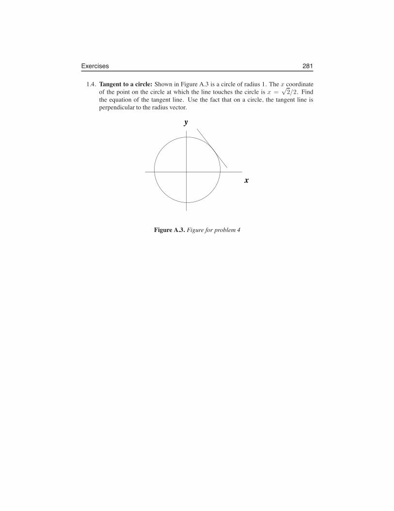
Exercises 281
1.4. Tangent to a circle: Shown in Figure A.3 is a circle of radius 1. The x coordinateof the point on the circle at which the line touches the circle is x =
√2/2. Find
the equation of the tangent line. Use the fact that on a circle, the tangent line isperpendicular to the radius vector.
x
y
Figure A.3. Figure for problem 4

282 Appendix A. A review of Straight Lines
Appendix B
A precalculus review
B.A Manipulating exponentsRecall that 2n = 2 · 2 . . . 2 (with n factors of 2).
This means that 2n ·2m = (2 ·2 . . .2) ·(2 ·2 . . .2) = 2n+m, where we have expandedthe product into n and then m factors of 2. Similarly, we can derive many properties ofmanipulations of exponents. A list of these appears below, and holes for any positive basea
1. 2a2b = 2a+b as with all similar exponent manipulations.
2. (2a)b = 2ab also stems from simple rules for manipulating exponents
3. 2x is a function that is defined, continuous, and differentiable for all real numbers x.
4. 2x > 0 for all values of x.
5. We define 20 = 1, and we also have that 21 = 2.
6. 2x → 0 for increasing negative values of x
7. 2x → ∞ for increasing positive values of x
B.B Manipulating logarithmsThe following properties hold for logarithms of any base. Since we have used the base 2 inour previous section, we keep the same base here as well Properties of the logarithm stemdirectly from properties of the exponential function, and include the following:
1. log2(ab) = log2(a) + log2(b)
2. log2(ab) = b log2(a)
3. log2(1/a) = log2(a−1) = − log2(a)
283

284 Appendix B. A precalculus review
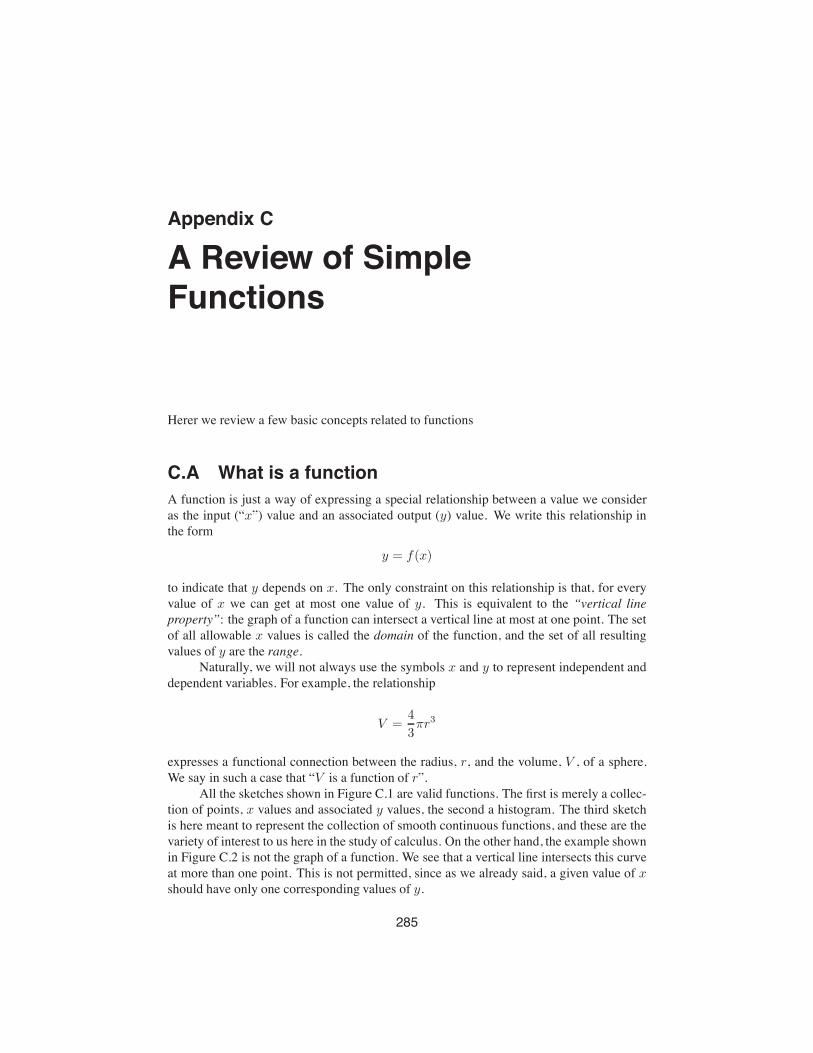
Appendix C
A Review of SimpleFunctions
Herer we review a few basic concepts related to functions
C.A What is a functionA function is just a way of expressing a special relationship between a value we consideras the input (“x”) value and an associated output (y) value. We write this relationship inthe form
y = f(x)
to indicate that y depends on x. The only constraint on this relationship is that, for everyvalue of x we can get at most one value of y. This is equivalent to the “vertical lineproperty”: the graph of a function can intersect a vertical line at most at one point. The setof all allowable x values is called the domain of the function, and the set of all resultingvalues of y are the range.
Naturally, we will not always use the symbols x and y to represent independent anddependent variables. For example, the relationship
V =4
3πr3
expresses a functional connection between the radius, r, and the volume, V , of a sphere.We say in such a case that “V is a function of r”.
All the sketches shown in Figure C.1 are valid functions. The first is merely a collec-tion of points, x values and associated y values, the second a histogram. The third sketchis here meant to represent the collection of smooth continuous functions, and these are thevariety of interest to us here in the study of calculus. On the other hand, the example shownin Figure C.2 is not the graph of a function. We see that a vertical line intersects this curveat more than one point. This is not permitted, since as we already said, a given value of xshould have only one corresponding values of y.
285
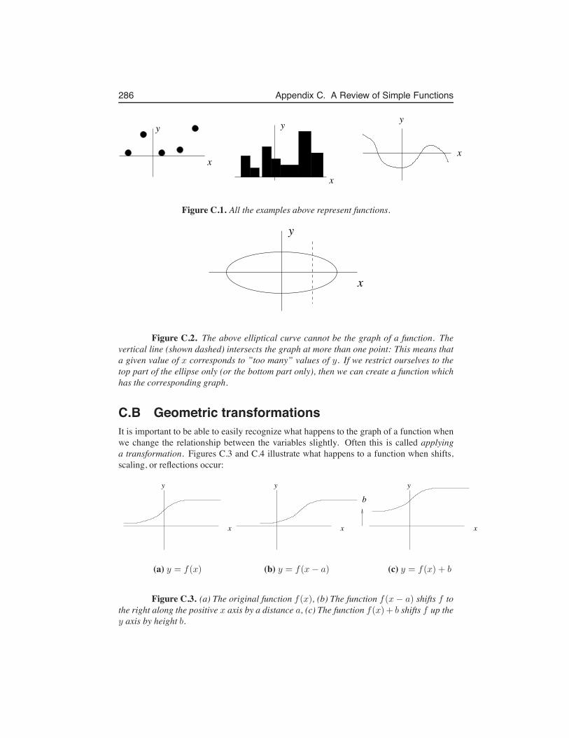
286 Appendix C. A Review of Simple Functions
x
x
x
yyy
Figure C.1. All the examples above represent functions.
x
y
Figure C.2. The above elliptical curve cannot be the graph of a function. Thevertical line (shown dashed) intersects the graph at more than one point: This means thata given value of x corresponds to ”too many” values of y. If we restrict ourselves to thetop part of the ellipse only (or the bottom part only), then we can create a function whichhas the corresponding graph.
C.B Geometric transformationsIt is important to be able to easily recognize what happens to the graph of a function whenwe change the relationship between the variables slightly. Often this is called applyinga transformation. Figures C.3 and C.4 illustrate what happens to a function when shifts,scaling, or reflections occur:
x
y
x
y
x
y
b
(a) y = f(x) (b) y = f(x− a) (c) y = f(x) + b
Figure C.3. (a) The original function f(x), (b) The function f(x− a) shifts f tothe right along the positive x axis by a distance a, (c) The function f(x) + b shifts f up they axis by height b.
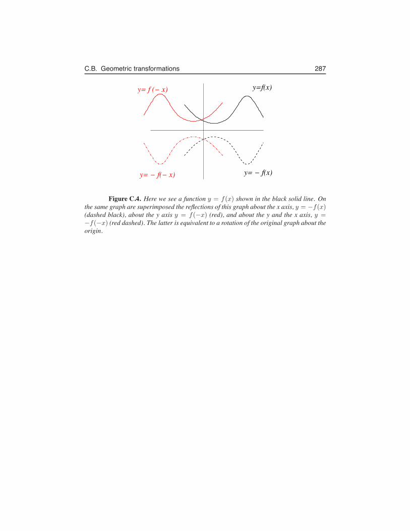
C.B. Geometric transformations 287
y= f (! x) y=f(x)
y= ! f(x)y= ! f(! x)
Figure C.4. Here we see a function y = f(x) shown in the black solid line. Onthe same graph are superimposed the reflections of this graph about the x axis, y = −f(x)(dashed black), about the y axis y = f(−x) (red), and about the y and the x axis, y =−f(−x) (red dashed). The latter is equivalent to a rotation of the original graph about theorigin.
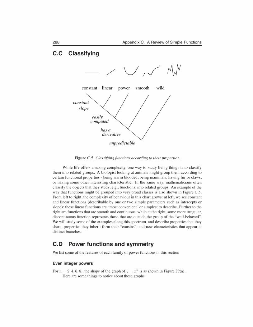
288 Appendix C. A Review of Simple Functions
C.C Classifying
constant linear power smooth wild
constantslope
easilycomputed
has aderivative
unpredictable
Figure C.5. Classifying functions according to their properties.
While life offers amazing complexity, one way to study living things is to classifythem into related groups. A biologist looking at animals might group them according tocertain functional properties - being warm blooded, being mammals, having fur or claws,or having some other interesting characteristic. In the same way, mathematicians oftenclassify the objects that they study, e.g., functions, into related groups. An example of theway that functions might be grouped into very broad classes is also shown in Figure C.5.From left to right, the complexity of behaviour in this chart grows: at left, we see constantand linear functions (describable by one or two simple parameters such as intercepts orslope): these linear functions are “most convenient” or simplest to describe. Further to theright are functions that are smooth and continuous, while at the right, some more irregular,discontinuous function represents those that are outside the group of the “well-behaved”.We will study some of the examples along this spectrum, and describe properties that theyshare, properties they inherit form their “cousins”, and new characteristics that appear atdistinct branches.
C.D Power functions and symmetryWe list some of the features of each family of power functions in this section
Even integer powers
For n = 2, 4, 6, 8.. the shape of the graph of y = xn is as shown in Figure ??(a).Here are some things to notice about these graphs:
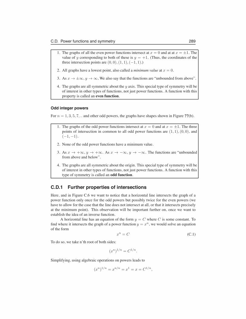
C.D. Power functions and symmetry 289
1. The graphs of all the even power functions intersect at x = 0 and at at x = ±1. Thevalue of y corresponding to both of these is y = +1. (Thus, the coordinates of thethree intersection points are (0, 0), (1, 1), (−1, 1).)
2. All graphs have a lowest point, also called a minimum value at x = 0.
3. As x → ±∞, y → ∞, We also say that the functions are “unbounded from above”.
4. The graphs are all symmetric about the y axis. This special type of symmetry will beof interest in other types of functions, not just power functions. A function with thisproperty is called an even function.
Odd integer powers
For n = 1, 3, 5, 7, .. and other odd powers, the graphs have shapes shown in Figure ??(b).
1. The graphs of the odd power functions intersect at x = 0 and at x = ±1. The threepoints of intersection in common to all odd power functions are (1, 1), (0, 0), and(−1,−1).
2. None of the odd power functions have a minimum value.
3. As x → +∞, y → +∞. As x → −∞, y → −∞. The functions are “unboundedfrom above and below”.
4. The graphs are all symmetric about the origin. This special type of symmetry will beof interest in other types of functions, not just power functions. A function with thistype of symmetry is called an odd function.
C.D.1 Further properties of intersectionsHere, and in Figure C.6 we want to notice that a horizontal line intersects the graph of apower function only once for the odd powers but possibly twice for the even powers (wehave to allow for the case that the line does not intersect at all, or that it intersects preciselyat the minimum point). This observation will be important further on, once we want toestablish the idea of an inverse function.
A horizontal line has an equation of the form y = C where C is some constant. Tofind where it intersects the graph of a power function y = xn, we would solve an equationof the form
xn = C (C.1)
To do so, we take n’th root of both sides:
(xn)1/n = C1/n.
Simplifying, using algebraic operations on powers leads to
(xn)1/n = xn/n = x1 = x = C1/n,
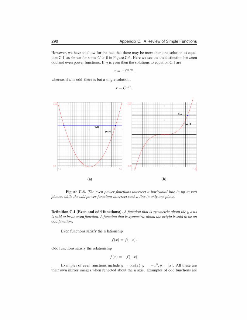
290 Appendix C. A Review of Simple Functions
However, we have to allow for the fact that there may be more than one solution to equa-tion C.1, as shown for some C > 0 in Figure C.6. Here we see the the distinction betweenodd and even power functions. If n is even then the solutions to equation C.1 are
x = ±C1/n,
whereas if n is odd, there is but a single solution,
x = C1/n.
y=x^2
y=C
-1.5 1.50.0
2.25
y=x^3
y=C
-1.5 1.5-2.25
2.25
(a) (b)
Figure C.6. The even power functions intersect a horizontal line in up to twoplaces, while the odd power functions intersect such a line in only one place.
Definition C.1 (Even and odd functions:). A function that is symmetric about the y axisis said to be an even function. A function that is symmetric about the origin is said to be anodd function.
Even functions satisfy the relationship
f(x) = f(−x).
Odd functions satisfy the relationship
f(x) = −f(−x).
Examples of even functions include y = cos(x), y = −x8, y = |x|. All these aretheir own mirror images when reflected about the y axis. Examples of odd functions are
C.D. Power functions and symmetry 291
y = sin(x), y = −x3, y = x. Each of these functions is its own double-reflection (about yand then x axes).
In a later calculus course, when we compute integrals, taking these symmetries intoaccount can help to simplify (or even avoid) calculations.
C.D.2 Optional: Combining even and odd functionsNot every function is either odd or even. However, if we start with symmetric functions,certain manipulations either preserve or reverse the symmetry.
Example C.2 Show that the product of an even and an odd function is an odd function.
Solution: Let f(x) be even. Then
f(x) = f(−x).
Let g(x) be an odd function. Then g(x) = −g(−x). We define h(x) to be the product ofthese two functions,
h(x) = f(x)g(x).
Using the properties of f and g,
f(x)g(x) = f(−x)[−g(−x)]
so, rearranging, we get
h(x) = f(x)g(x) = f(−x)[−g(−x)] = −[f(−x)g(−x)].
but this is just the same as −h(−x). We have established that
h(x) = −h(−x)
so that the new function is odd.A function is not always even or odd. Many functions are neither even nor odd.
However, by a little trick, we can show that given any function, y = f(x), we can write itas a sum of an even and an odd function.
Hint: Suppose f(x) is not an even nor an odd function. Consider defining the two associ-ated functions:
fe(x) =1
2(f(x) + f(−x)),
andf0(x) =
1
2(f(x)− f(−x)).
(Can you draw a sketch of what these would look like for the function given in Fig-ure C.3(a)?) Show that fe(x) is even and that f0(x) is odd. Now show that
f(x) = fe(x) + f0(x).
292 Appendix C. A Review of Simple Functions
C.E Inverse functions and fractional powersSuppose we are given a function expressed in the form
y = f(x).
What this implies, is that x is the independent variable, and y is obtained from it by evalu-ating a function, i.e. by using the “rule” or operation specified by that function. The abovemathematical statement expresses a certain relationship between the two variables, x andy, in which the roles are distinct. x is a value we pick, and y is then calculated from it.
However, sometimes we can express a relationship in more than one way: as anexample, if the connection between x and y is simple squaring, then provided x > 0, wemight write either
y = x2
orx = y1/2 =
√y
to express the same relationship. In other words
y = x2 ⇔ x =√y.
Observe that we have used two distinct functions in describing the relationship fromthe two points of view: One function involves squaring and the other takes a square root.We may also notice that for x > 0
f(g(x)) = (√x)2 = x
g(f(x)) =√
(x2) = x
i.e. that these two functions invert each other’s effect.Functions that satisfy
y = f(x) ⇔ x = g(y)
are said to be inverse functions. We will often use the notation
f−1(x)
to denote the function that acts as an inverse function to f(x).
C.E.1 Graphical property of inverse functionsThe graph of an inverse function y = f−1(x) is geometrically related to the graph of theoriginal function: it is a reflection of y = f(x) about the 45◦ line, y = x. This relationshipis shown in figure C.7 for a pair of functions f and f−1.
But why should this be true? The idea is as follows: Suppose that (a, b) is anypoint on the graph of y = f(x). This means that b = f(a). That, in turn, implies thata = f−1(b), which then tells us that (b, a) must be a point on the graph of f−1(x). But thepoints (a, b) and (b, a) are related by reflection about the line y = x. This is true for anyarbitrary point, and so must be true for all points on the graphs of the two functions.
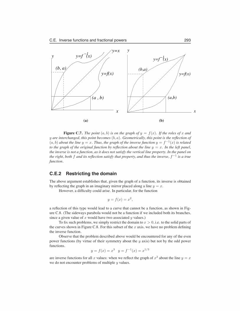
C.E. Inverse functions and fractional powers 293
x
yy=x
y=f(x)
y=f (x)!1
(a , b)
(b, a)
!1
y
x
(a,b)
(b,a)y=f(x)
y=f (x)
(a) (b)
Figure C.7. The point (a, b) is on the graph of y = f(x). If the roles of x andy are interchanged, this point becomes (b, a). Geometrically, this point is the reflection of(a, b) about the line y = x. Thus, the graph of the inverse function y = f−1(x) is relatedto the graph of the original function by reflection about the line y = x. In the left panel,the inverse is not a function, as it does not satisfy the vertical line property. In the panel onthe right, both f and its reflection satisfy that property, and thus the inverse, f−1 is a truefunction.
C.E.2 Restricting the domainThe above argument establishes that, given the graph of a function, its inverse is obtainedby reflecting the graph in an imaginary mirror placed along a line y = x.
However, a difficulty could arise. In particular, for the function
y = f(x) = x2,
a reflection of this type would lead to a curve that cannot be a function, as shown in Fig-ure C.8. (The sideways parabola would not be a function if we included both its branches,since a given value of x would have two associated y values.)
To fix such problems, we simply restrict the domain to x > 0, i.e. to the solid parts ofthe curves shown in Figure C.8. For this subset of the x axis, we have no problem definingthe inverse function.
Observe that the problem described above would be encountered for any of the evenpower functions (by virtue of their symmetry about the y axis) but not by the odd powerfunctions.
y = f(x) = x3 y = f−1(x) = x1/3
are inverse functions for all x values: when we reflect the graph of x3 about the line y = xwe do not encounter problems of multiple y values.
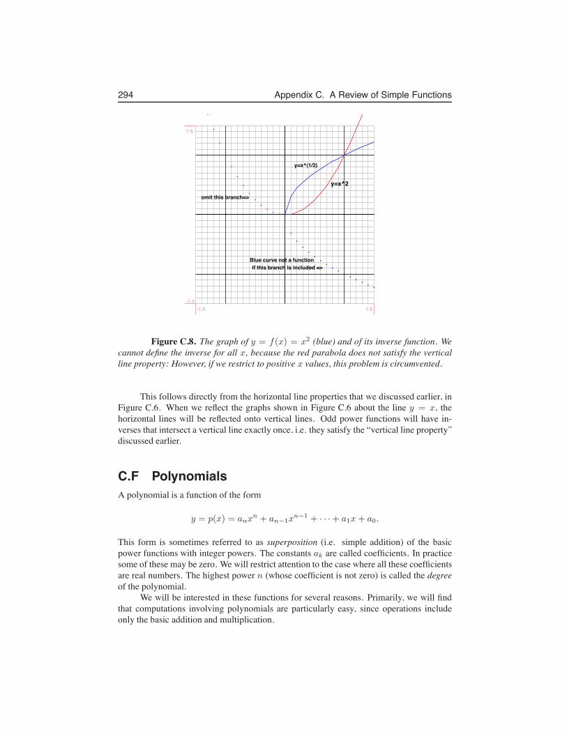
294 Appendix C. A Review of Simple Functions
y=x^2
y=x^(1/2)
omit this branch=>
Blue curve not a functionif this branch is included =>
-1.5 1.5-1.5
1.5
Figure C.8. The graph of y = f(x) = x2 (blue) and of its inverse function. Wecannot define the inverse for all x, because the red parabola does not satisfy the verticalline property: However, if we restrict to positive x values, this problem is circumvented.
This follows directly from the horizontal line properties that we discussed earlier, inFigure C.6. When we reflect the graphs shown in Figure C.6 about the line y = x, thehorizontal lines will be reflected onto vertical lines. Odd power functions will have in-verses that intersect a vertical line exactly once, i.e. they satisfy the “vertical line property”discussed earlier.
C.F PolynomialsA polynomial is a function of the form
y = p(x) = anxn + an−1x
n−1 + · · ·+ a1x+ a0.
This form is sometimes referred to as superposition (i.e. simple addition) of the basicpower functions with integer powers. The constants ak are called coefficients. In practicesome of these may be zero. We will restrict attention to the case where all these coefficientsare real numbers. The highest power n (whose coefficient is not zero) is called the degreeof the polynomial.
We will be interested in these functions for several reasons. Primarily, we will findthat computations involving polynomials are particularly easy, since operations includeonly the basic addition and multiplication.
C.F. Polynomials 295
C.F.1 Features of polynomials• Zeros of a polynomial are values of x such that
y = p(x) = 0.
If p(x) is quadratic (a polynomial of degree 2) then the quadratic formula gives asimple way of finding roots of this equation (also called “zeros” of the polynomial).Generally, for most polynomials of degree higher than 5, there is no analytical recipefor finding zeros. Geometrically, zeros are places where the graph of the functiony = p(x) crosses the x axis. We will exploit this fact much later in the course toapproximate the values of the zeros using Newton’s Method.
• Critical Points: Places on the graph where the value of the function is locally largerthan those nearby (local maxima) or smaller than those nearby (local minima) will beof interest to us. Calculus will be one of the main tools for detecting and identifyingsuch places.
• Behaviour for very large x: All polynomials are unbounded as x → ∞ and asx → −∞. In fact, for large enough values of x, we have seen that the power functiony = f(x) = xn with the largest power, n, dominates over other power functions withsmaller powers.For
p(x) = anxn + an−1x
n−1 + · · ·+ a1x+ a0
the first (highest power) term will dominate for large x. Thus for large x (whetherpositive or negative)
p(x) ≈ anxn for large x.
• Behaviour for small x: Close to the origin, we have seen that power functions withsmallest powers dominate. This means that for x ≈ 0 the polynomial is governed bythe behaviour of the smallest (non-zero coefficient) power, i.e,
p(x) ≈ a1x+ a0 for small x.
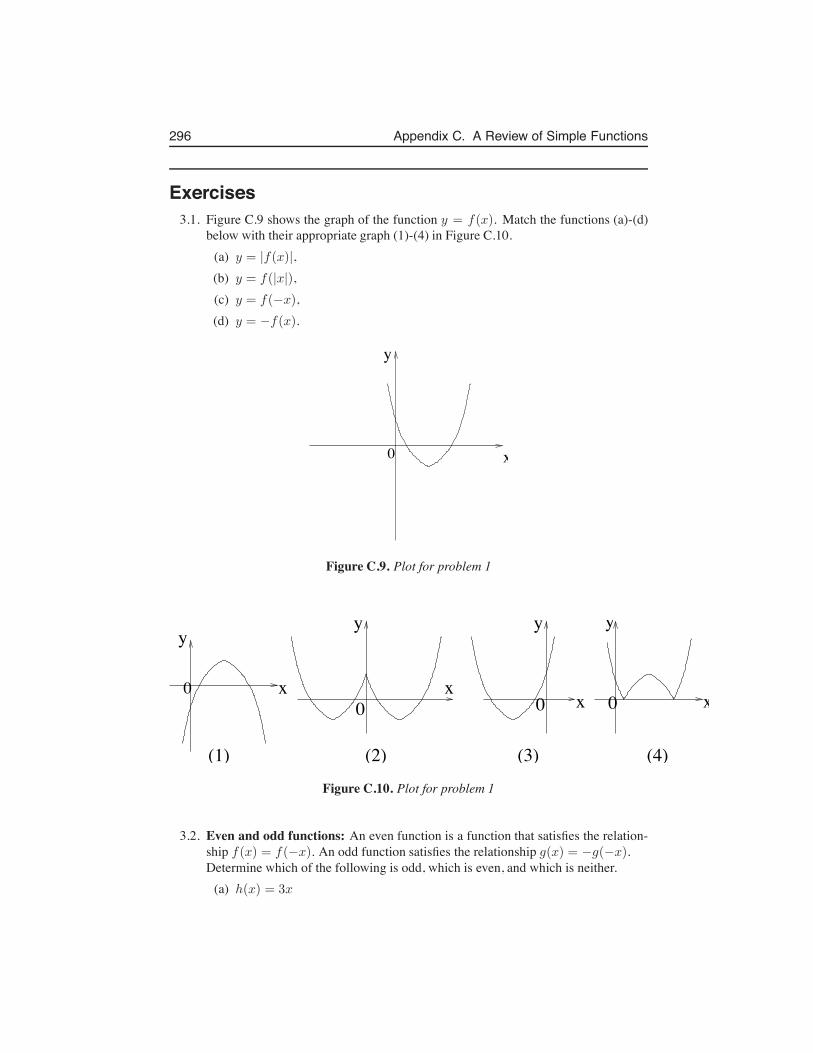
296 Appendix C. A Review of Simple Functions
Exercises3.1. Figure C.9 shows the graph of the function y = f(x). Match the functions (a)-(d)
below with their appropriate graph (1)-(4) in Figure C.10.(a) y = |f(x)|,(b) y = f(|x|),(c) y = f(−x),(d) y = −f(x).
0
y
x
Figure C.9. Plot for problem 1
xx
y
x
y
x
y
(1) (2) (3) (4)
y
0 000
Figure C.10. Plot for problem 1
3.2. Even and odd functions: An even function is a function that satisfies the relation-ship f(x) = f(−x). An odd function satisfies the relationship g(x) = −g(−x).Determine which of the following is odd, which is even, and which is neither.
(a) h(x) = 3x
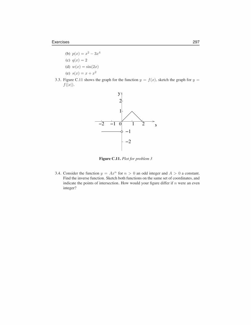
Exercises 297
(b) p(x) = x2 − 3x4
(c) q(x) = 2
(d) w(x) = sin(2x)
(e) s(x) = x+ x2
3.3. Figure C.11 shows the graph for the function y = f(x), sketch the graph for y =f(|x|).
0
2
!2 1 2!1
1
x
y
!1
!2
Figure C.11. Plot for problem 3
3.4. Consider the function y = Axn for n > 0 an odd integer and A > 0 a constant.Find the inverse function. Sketch both functions on the same set of coordinates, andindicate the points of intersection. How would your figure differ if n were an eveninteger?

298 Appendix C. A Review of Simple Functions
Appendix D
Limits
We have surreptitiously introduced some notation involving limits without carefully defin-ing what was meant. Here, such technical matters are briefly discussed.
The concept of a limit helps us to describe the behaviour of a function close to somepoint of interest. This proves to be most useful in the case of functions that are either notcontinuous, or not defined somewhere. We will use the notation
limx→a
f(x)
to denote the value that the function f approaches as x gets closer and closer to the valuea.
D.A Limits for continuous functionsIf x = a is a point at which the function is defined and continuous (informally, has no“breaks in its graph”) the value of the limit and the value of the function at a point are thesame, i.e.
If f is continuous at x = a then
limx→a
f(x) = f(a).
Example D.1 Find limx→0
f(x) for the function y = f(x) = 10
Solution: This function is continuous (and constant) everywhere. In fact, the value of thefunction is independent of x. We conclude immediately that
limx→0
f(x) = limx→0
10 = 10.
Example D.2 Find limx→0
f(x) for the function y = f(x) = sin(x).
299
300 Appendix D. Limits
Solution: This function is a continuous trigonometric function, and has the value sin(0) =0 at the origin. Thus
limx→0
f(x) = limx→0
sin(x) = 0
Power functions are continuous everywhere. This motivates the next example.
Example D.3 Compute the limit limx→0
xn where n is a positive integer.
Solution: The function in question, f(x) = xn is a simple power function that is continu-ous everywhere. Further, f(0) = 0. Hence the limit as x → 0 coincides with the value ofthe function oat that point, so
limx→0
xn = 0.
D.B Properties of limitsSuppose we are given two functions, f(x) and g(x). We will also assume that both func-tions have (finite) limits at the point x = a. Then the following statements follow.
1.limx→a
(f(x) + g(x)) = limx→a
f(x) + limx→a
g(x)
2.limx→a
(cf(x)) = c limx→a
f(x)
3.limx→a
(f(x) · g(x)) =(
limx→a
f(x))
·(
limx→a
g(x))
4. Provided that limx→a
g(x) $= 0, we also have that
limx→a
(
f(x)
g(x)
)
=
(
limx→a
f(x)
limx→a
g(x)
)
.
The first two statements are equivalent to linearity of the process of computing alimit.
Example D.4 Find limx→2
f(x) for the function y = f(x) = 2x2 − x3.
Solution: Since this function is a polynomial, and so continuous everywhere, we can sim-ply plug in the relevant value of x, i.e.
limx→2
(
2x2 − x3)
= 2 · 22 − 23 = 0.
Thus when x gets closer to 2, the value of the function gets closer to 0. (In fact, the valueof the limit is the same as the value of the function at the given point.)
D.C. Limits of rational functions 301
D.C Limits of rational functionsD.C.1 Case 1: Denominator nonzeroWe first consider functions that are the quotient of two polynomials, y = f(x)/g(x) atpoints were g(x) $= 0. This allows us to apply Property 4 of limits together with whatwe have learned about the properties of power functions and polynomials. Much of thisdiscussion is related to the properties of power functions and dominance of lower (higher)powers at small (large) values of x, as discussed in Chapter 1. In the examples below, weconsider both limits at the origin (at x = 0) and at infinity (for x → ∞). The latter means“very large x”. See Section 1.5 for examples of the informal version of the same reasoningused to reach the same conclusions.
Example D.5 Find the limit as x → 0 and as x → ∞ of the quotients
(a)Kx
kn + x, (b)
Axn
an + xn.
Solution: We recognize (a) as an example of the Michaelis Menten kinetics, found in (1.2)and (b) as a Hill function in (1.3) of Chapter 1. We now compute, first for x → 0,
(a) limx→0
Kx
kn + x= 0, (b) lim
x→0
Axn
an + xn= 0.
This follows from the fact that, provided a, kn $= 0, both functions are continuous at x = 0,so that their limits are the same as the actual values attained by the functions. Now forx → ∞
(a) limx→∞
Kx
kn + x= lim
x→∞
Kx
x= K, (b) lim
x→∞
Axn
an + xn= lim
x→∞
Axn
xn= A.
This follows from the fact that the constants kn, an are always “swamped out” by the valueof x as x → ∞, allowing us to obtain the result. Other than the formal limit notation, thereis nothing new here that we have not already discussed in Sections 1.6.
Below we apply similar reasoning to other examples of rational functions.
Example D.6 Find the limit as x → 0 and as x → ∞ of the quotients
(a) 3x2
9 + x2, (b) 1 + x
1 + x3.
Solution: For part (a) we note that as x → ∞, the quotient approaches 3x2/x2 = 3. Asx → 0, both numerator and denominator are defined and the denominator is nonzero, sowe can use the 4th property of limits. We thus find that
(a) limx→∞
3x2
9 + x2= 3, lim
x→0
3x2
9 + x2= 0,
302 Appendix D. Limits
For part (b), we use the fact that as x → ∞, the limit approaches x/x3 = x−2 → 0. Asx → 0 we can apply property 4 yet again to compute the (finite) limit, so that
(b) limx→∞
1 + x
1 + x3, lim
x→0
1 + x
1 + x3.
Example D.7 Find the limits of the following function at 0 and ∞
y =x4 − 3x2 + x− 1
x5 + x.
Solution: for x → ∞ powers with the largest power dominate, whereas for x → 0, smallerpowers dominate. Hence, we find
limx→∞
x4 − 3x2 + x− 1
x5 + x= lim
x→∞
x4
x5= lim
x→∞
1
x= 0.
limx→0
x4 − 3x2 + x− 1
x5 + x= lim
x→0
−1
x= − lim
x→0
1
x= ∞
So in the latter case, the limit does not exist.
D.C.2 Case 2: zero in the denominator and “holes” in a graphIn the previous examples, evaluating the limit, where it existed, was as simple as pluggingthe appropriate value of x into the function itself. The next example shows that this is notalways possible.
Example D.8 Compute the limit as x → 4 of the function f(x) = 1/(x− 4)
Solution: This function has a vertical asymptote at x = 4. Indeed, the value of the functionshoots off to +∞ if we approach x = 4 from above, and −∞ if we approach the same pointfrom below. We say that the limit does not exist in this case.
Example D.9 Compute the limit as x → −1 of the function f(x) = x/(x2 − 1)
Solution: We compute
limx→−1
x
x2 − 1= lim
x→−1
x
(x − 1)(x+ 1)
It is evident (even before factoring as we have done) that this function has a vertical asymp-tote at x = −1 where the denominator approaches zero. Hence, the limit does not exist.
Next, we describe an extremely important example where the function has a “hole” inits graph, but where a finite limit exists. This kind of limit plays a huge role in the definitionof a derivative.
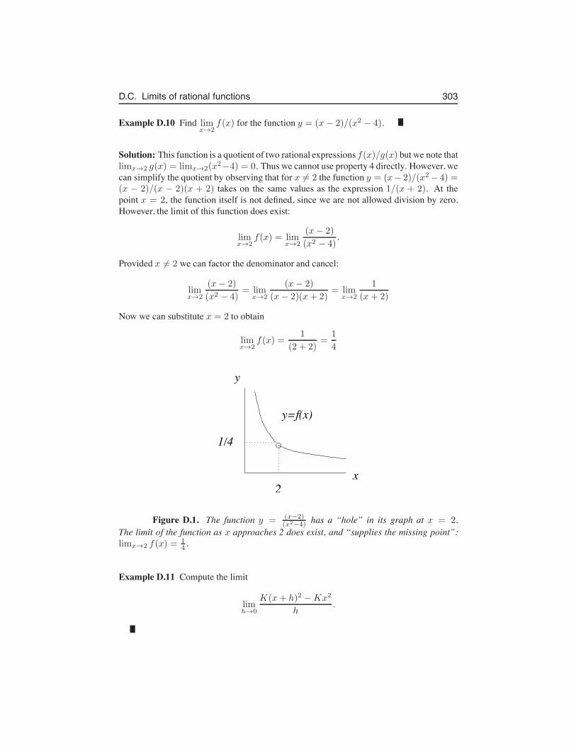
D.C. Limits of rational functions 303
Example D.10 Find limx→2
f(x) for the function y = (x− 2)/(x2 − 4).
Solution: This function is a quotient of two rational expressions f(x)/g(x) but we note thatlimx→2 g(x) = limx→2(x2−4) = 0. Thus we cannot use property 4 directly. However, wecan simplify the quotient by observing that for x $= 2 the function y = (x− 2)/(x2− 4) =(x − 2)/(x − 2)(x + 2) takes on the same values as the expression 1/(x + 2). At thepoint x = 2, the function itself is not defined, since we are not allowed division by zero.However, the limit of this function does exist:
limx→2
f(x) = limx→2
(x− 2)
(x2 − 4).
Provided x $= 2 we can factor the denominator and cancel:
limx→2
(x− 2)
(x2 − 4)= lim
x→2
(x− 2)
(x− 2)(x+ 2)= lim
x→2
1
(x + 2)
Now we can substitute x = 2 to obtain
limx→2
f(x) =1
(2 + 2)=
1
4
y
2
1/4
y=f(x)
x
Figure D.1. The function y = (x−2)(x2−4) has a “hole” in its graph at x = 2.
The limit of the function as x approaches 2 does exist, and “supplies the missing point”:limx→2 f(x) =
14 .
Example D.11 Compute the limit
limh→0
K(x+ h)2 −Kx2
h.
304 Appendix D. Limits
Solution: This is a calculation we would perform to compute the derivative of the functiony = Kx2 from the definition of the derivative. Details have already been displayed in Ex-ample 2.10. The essential idea is that we expand the numerator and simplify algebraicallyas follows:
limh→0
K(2xh+ h2)
h= lim
h→0K(2x+ h) = 2Kx.
Even though the quotient is not defined at the value h = 0 (as the denominator is zerothere), the limit exists, and hence the derivative can be defined. See also Example 4.1 for asimilar calculation for the function Kx3.
D.D Right and left sided limitsSome functions are discontinuous at a point, but we may still be able to define a limit thatthe function attains as we approach that point from the right or from the left. (This isequivalent to gradually decreasing or gradually increasing x as we get closer to the pointof interest.
Consider the function
f(x) =
{
0 if x < 0;1 if x > 0.
This is a step function, whose values is 0 for negative real numbers, and 1 for positive realnumbers. The function is not even defined at the point x = 0 and has a jump in its graph.However, we can still define a right and a left limit as follows:
limx→+0
f(x) = 0, limx→−0
f(x) = 1.
That is, the limit as we approach from the right is 0 whereas from the left it is 1. We alsostate the following result:
If f(x) has a right and a left limit at a point x = a and if those limitsare equal, then we say that the limit at x = a exists, and we write
limx→+a
f(x) = limx→−a
f(x) = limx→a
f(x)
Example D.12 Find limx→π/2
f(x) for the function y = f(x) = tan(x).
Solution: The function tan(x) = sin(x)/ cos(x) cannot be continuous at x = π/2 becausecos(x) in the denominator takes on the value of zero at the point x = π/2. Moreover, thevalue of this function becomes unbounded (grows without a limit) as x → π/2. We say inthis case that “the limit does not exist”. We sometimes use the notation
limx→π/2
tan(x) = ±∞.
(We can distinguish the fact that the function approaches +∞ as x approaches π/2 frombelow, and −∞ as x approaches π/2 from higher values.
D.E. Limits at infinity 305
D.E Limits at infinityWe can also describe the behaviour “at infinity” i.e. the trend displayed by a function forvery large (positive or negative) values of x. We consider a few examples of this sort below.
Example D.13 Find limx→∞
f(x) for the function y = f(x) = x3 − x5 + x.
Solution: All polynomials grow in an unbounded way as x tends to very large values. Wecan determine whether the function approaches positive or negative unbounded values bylooking at the coefficient of the highest power of x, since that power dominates at large xvalues. In this example, we find that the term −x5 is that highest power. Since this has anegative coefficient, the function will approach unbounded negative values as x gets largerin the positive direction, i.e.
limx→∞
x3 − x5 + x = limx→∞
−x5 = −∞.
Example D.14 Determine the following two limits:
(a) limx→∞
e−2x, (b) limx→−∞
e5x,
Solution: The function y = e−2x becomes arbitrarily small as x → ∞. The functiony = e5x becomes arbitrarily small as x → −∞. Thus we have
(a) limx→∞
e−2x = 0, (b) limx→−∞
e5x = 0.
Example D.15 Find the limits below:
(a) limx→∞
x2e−2x, (b) limx→0
1
xe−x,
Solution: For part (a) we state here the fact that as x → ∞, the exponential function withnegative exponent decays to zero faster than any power function increases. For part (b) wenote that for the quotient e−x/x we have that as x → 0 the top satisfies e−x → e0 = 1,while the denominator has x → 0. Thus the limit at x → 0 cannot exist. We find that
(a) limx→∞
x2e−2x = 0, (b) limx→0
1
xe−x = ∞,
D.F Summary of special limitsAs a reference, in the table below, we collect some of the special limits that are useful in avariety of situations.
We can summarize the information in this table informally as follows:
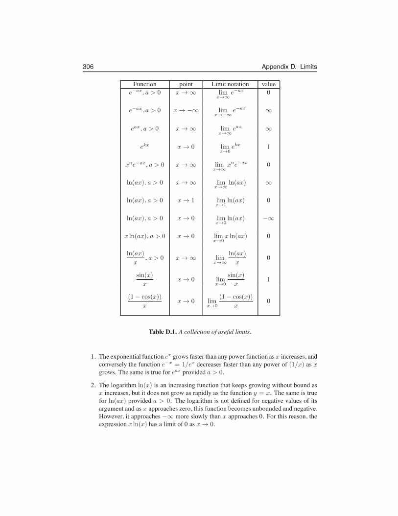
306 Appendix D. Limits
Function point Limit notation valuee−ax, a > 0 x → ∞ lim
x→∞e−ax 0
e−ax, a > 0 x → −∞ limx→−∞
e−ax ∞
eax, a > 0 x → ∞ limx→∞
eax ∞
ekx x → 0 limx→0
ekx 1
xne−ax, a > 0 x → ∞ limx→∞
xne−ax 0
ln(ax), a > 0 x → ∞ limx→∞
ln(ax) ∞
ln(ax), a > 0 x → 1 limx→1
ln(ax) 0
ln(ax), a > 0 x → 0 limx→0
ln(ax) −∞
x ln(ax), a > 0 x → 0 limx→0
x ln(ax) 0
ln(ax)
x, a > 0 x → ∞ lim
x→∞
ln(ax)
x0
sin(x)
xx → 0 lim
x→0
sin(x)
x1
(1− cos(x))
xx → 0 lim
x→0
(1 − cos(x))
x0
Table D.1. A collection of useful limits.
1. The exponential function ex grows faster than any power function as x increases, andconversely the function e−x = 1/ex decreases faster than any power of (1/x) as xgrows. The same is true for eax provided a > 0.
2. The logarithm ln(x) is an increasing function that keeps growing without bound asx increases, but it does not grow as rapidly as the function y = x. The same is truefor ln(ax) provided a > 0. The logarithm is not defined for negative values of itsargument and as x approaches zero, this function becomes unbounded and negative.However, it approaches −∞ more slowly than x approaches 0. For this reason, theexpression x ln(x) has a limit of 0 as x → 0.
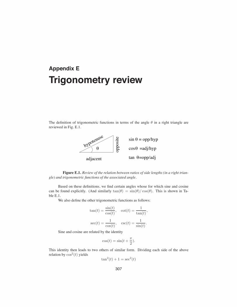
Appendix E
Trigonometry review
The definition of trigonometric functions in terms of the angle θ in a right triangle arereviewed in Fig. E.1.
adjacent
hypotenuse
# oppo
site sin = opp/hyp
cos =adj/hyp
tan =opp/adj
#
#
#
Figure E.1. Review of the relation between ratios of side lengths (in a right trian-gle) and trigonometric functions of the associated angle.
Based on these definitions, we find certain angles whose for which sine and cosinecan be found explicitly. (And similarly tan(θ) = sin(θ)/ cos(θ). This is shown in Ta-ble E.1.
We also define the other trigonometric functions as follows:
tan(t) =sin(t)
cos(t), cot(t) =
1
tan(t),
sec(t) =1
cos(t), csc(t) =
1
sin(t).
Sine and cosine are related by the identity
cos(t) = sin(t+π
2).
This identity then leads to two others of similar form. Dividing each side of the aboverelation by cos2(t) yields
tan2(t) + 1 = sec2(t)
307
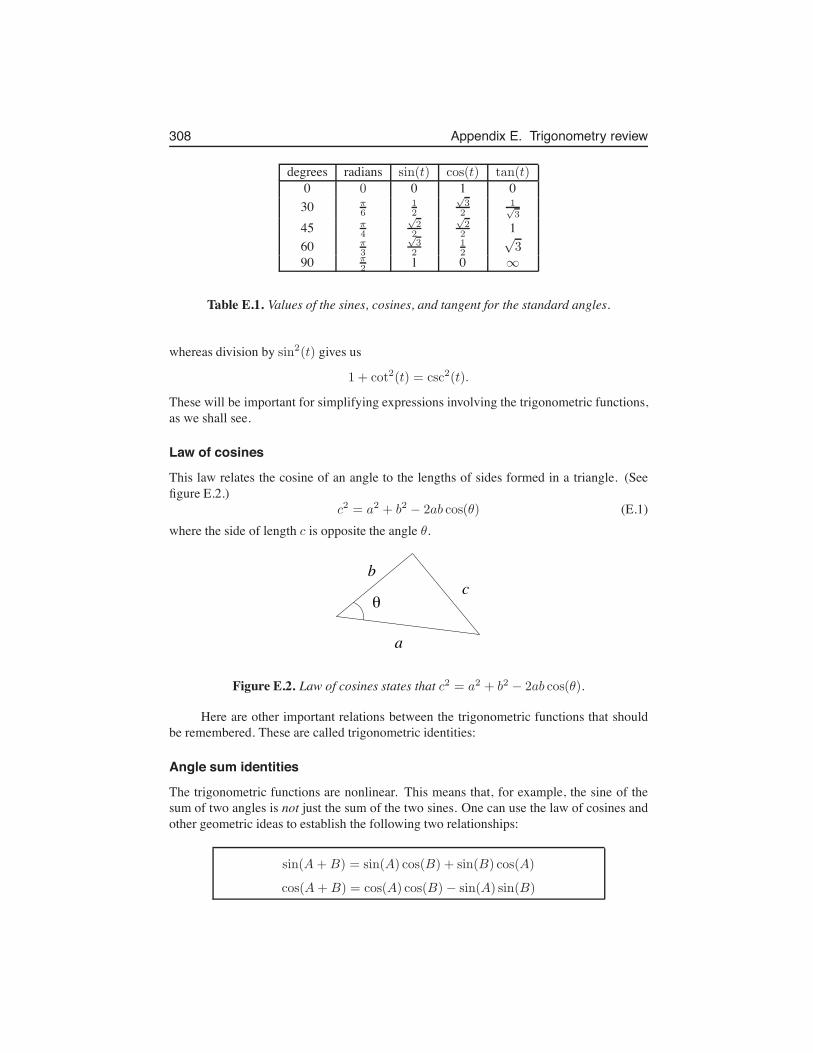
308 Appendix E. Trigonometry review
degrees radians sin(t) cos(t) tan(t)0 0 0 1 0
30 π6
12
√32
1√3
45 π4
√22
√22 1
60 π3
√32
12
√3
90 π2 1 0 ∞
Table E.1. Values of the sines, cosines, and tangent for the standard angles.
whereas division by sin2(t) gives us
1 + cot2(t) = csc2(t).
These will be important for simplifying expressions involving the trigonometric functions,as we shall see.
Law of cosines
This law relates the cosine of an angle to the lengths of sides formed in a triangle. (Seefigure E.2.)
c2 = a2 + b2 − 2ab cos(θ) (E.1)where the side of length c is opposite the angle θ.
a
bc
θ
Figure E.2. Law of cosines states that c2 = a2 + b2 − 2ab cos(θ).
Here are other important relations between the trigonometric functions that shouldbe remembered. These are called trigonometric identities:
Angle sum identities
The trigonometric functions are nonlinear. This means that, for example, the sine of thesum of two angles is not just the sum of the two sines. One can use the law of cosines andother geometric ideas to establish the following two relationships:
sin(A+B) = sin(A) cos(B) + sin(B) cos(A)
cos(A+B) = cos(A) cos(B)− sin(A) sin(B)
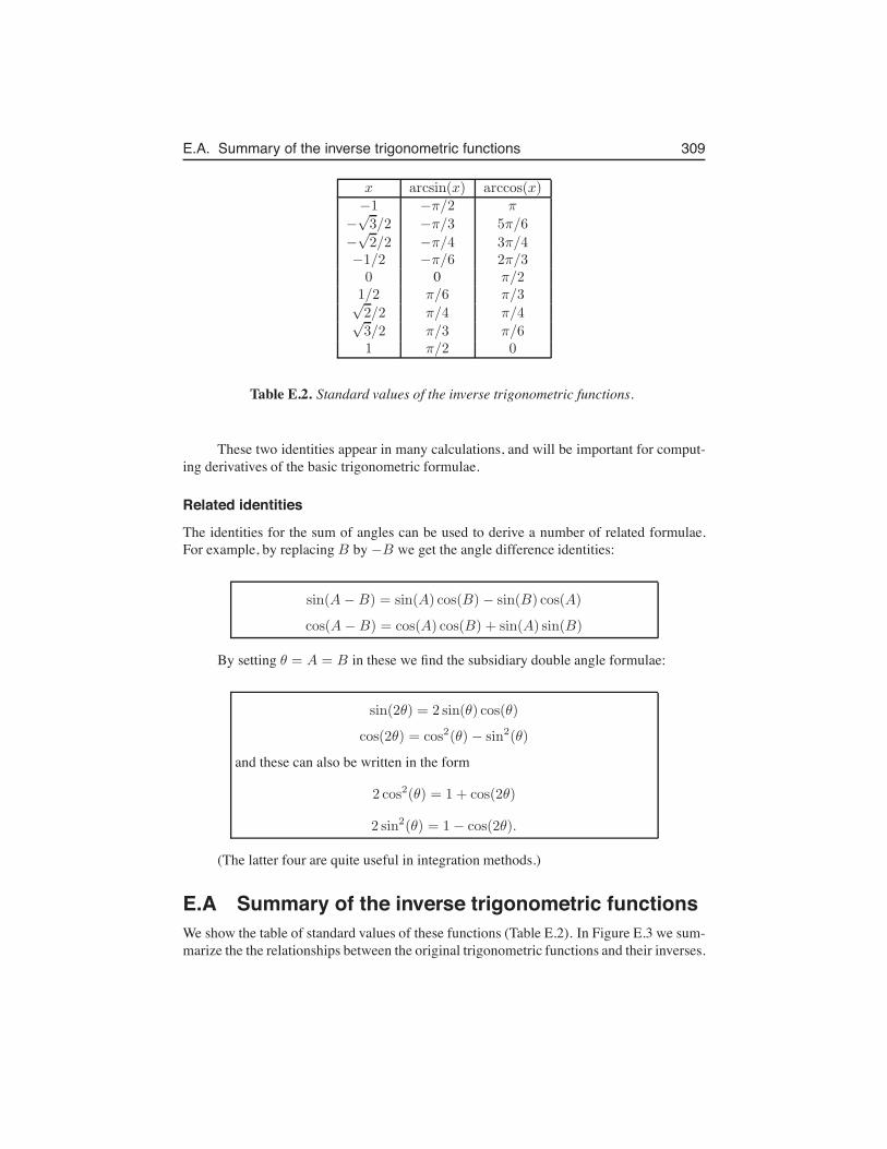
E.A. Summary of the inverse trigonometric functions 309
x arcsin(x) arccos(x)−1 −π/2 π
−√3/2 −π/3 5π/6
−√2/2 −π/4 3π/4
−1/2 −π/6 2π/30 0 π/2
1/2 π/6 π/3√2/2 π/4 π/4√3/2 π/3 π/61 π/2 0
Table E.2. Standard values of the inverse trigonometric functions.
These two identities appear in many calculations, and will be important for comput-ing derivatives of the basic trigonometric formulae.
Related identities
The identities for the sum of angles can be used to derive a number of related formulae.For example, by replacing B by −B we get the angle difference identities:
sin(A−B) = sin(A) cos(B)− sin(B) cos(A)
cos(A−B) = cos(A) cos(B) + sin(A) sin(B)
By setting θ = A = B in these we find the subsidiary double angle formulae:
sin(2θ) = 2 sin(θ) cos(θ)
cos(2θ) = cos2(θ)− sin2(θ)
and these can also be written in the form
2 cos2(θ) = 1 + cos(2θ)
2 sin2(θ) = 1− cos(2θ).
(The latter four are quite useful in integration methods.)
E.A Summary of the inverse trigonometric functionsWe show the table of standard values of these functions (Table E.2). In Figure E.3 we sum-marize the the relationships between the original trigonometric functions and their inverses.
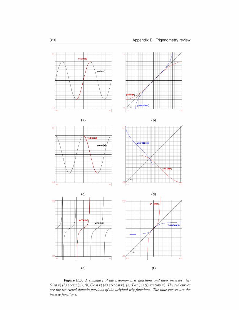
310 Appendix E. Trigonometry review
y=sin(x)
y=Sin(x)
-6.3 6.3-1.5
1.5
y=x
y=Sin(x)
y=arcsin(x)
-1.5 1.5-1.5
1.5
(a) (b)
y=cos(x)
y=Cos(x)
-6.3 6.3-1.5
1.5
y=x
y=Cos(x)
y=arccos(x)
-1.0 3.1-1.0
3.1
(c) (d)
y=tan(x)y=Tan(x)
-6.5 6.5-10.0
10.0
y=x
y=Tan(x)
y=arctan(x)
-6.3 6.3-6.3
6.3
(e) (f)
Figure E.3. A summary of the trigonometric functions and their inverses. (a)Sin(x) (b) arcsin(x), (b) Cos(x) (d) arccos(x), (e) Tan(x) (f) arctan(x). The red curvesare the restricted domain portions of the original trig functions. The blue curves are theinverse functions.
Appendix F
Short Answers toProblems
311

312 Appendix F. Short Answers to Problems
F..1 Answers to Chapter 1 Problems• Problem 1.1:
(a) Stretched in y direction by factor A; (b) Shifted up by a; (c) Shifted in positive xdirection by b.
• Problem 1.2:Not Provided
• Problem 1.3:y = xn; y = x−n; y = x1/n, n = 2, 4, 6, . . .; y = x−n, n = 1, 2, 3, . . .
• Problem 1.4:(a) x = 0, (3/2)1/3; (b) x = 0, x = ±
√
1/4.
• Problem 1.5:if m− n even: x = ±
(
AB
)1/(m−n), x = 0; if m− n odd: x =
(
AB
)1/(m−n), x = 0
• Problem 1.6:(a) (0, 0) and (1, 1); (b) (0, 0); (c) (
√72 , 3
4 ), (−√72 , 3
4 ), and (0,−1).
• Problem 1.7:m > −1
• Problem 1.8:Not Provided
• Problem 1.9:
x =
(
B
A
)1
b−a
• Problem 1.10:(a) x = 0, −1, 3; (b) x = 1; (c) x = −2, 1/3; (d) x = 1.
• Problem 1.11:(b) a < 0: x = 0; a ≥ 0: x = 0, ±a1/4; (c) a > 0.
• Problem 1.12:Not Provided
• Problem 1.13:
(a) V ; (b) VS
=1
6a, a > 0; (c) a = V
13 ; a = (16S)
12 ; a = 10 cm; a =
√153 cm.
• Problem 1.14:(a) V ; (b) r
3; (c) r =
(
34π
)1/3V 1/3; r =
(
14π
)1/2S1/2; r ≈ 6.2035 cm; r ≈
0.8921 cm.
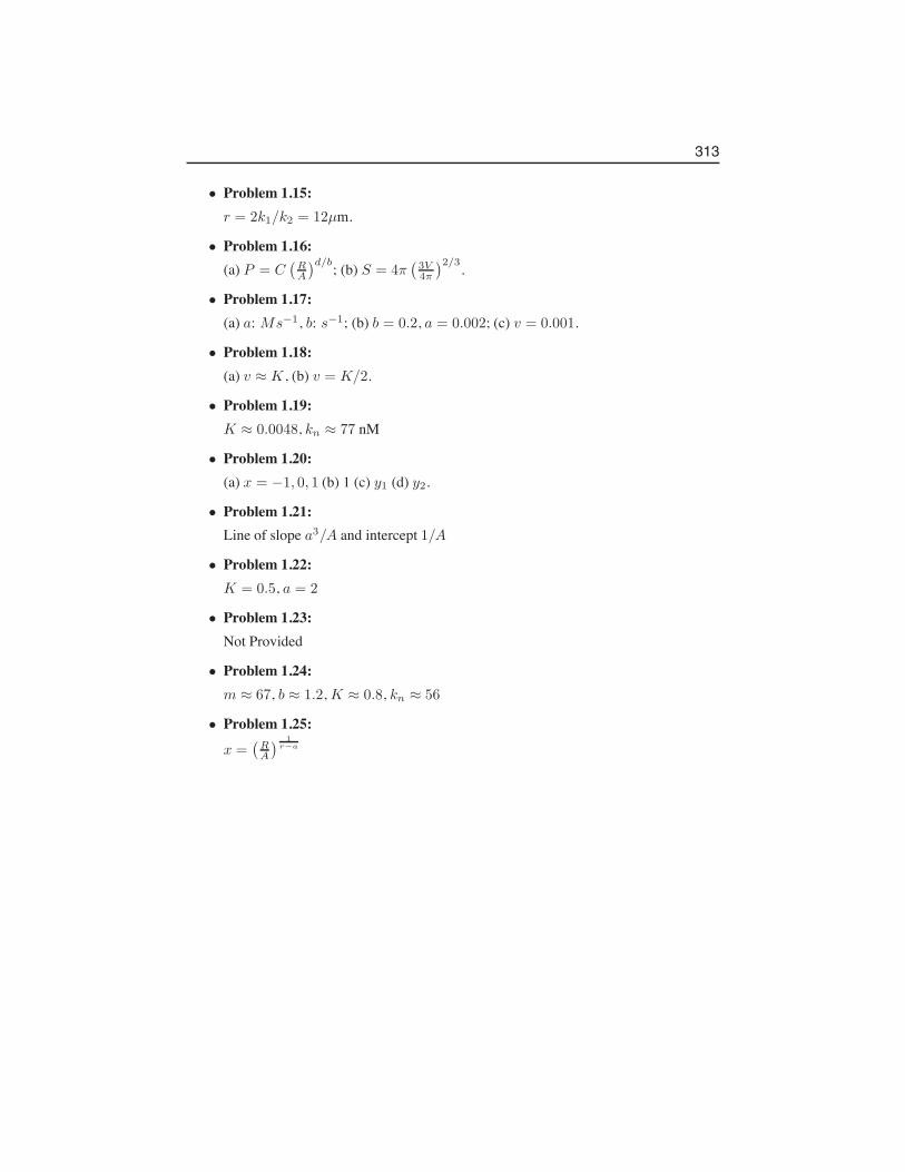
313
• Problem 1.15:r = 2k1/k2 = 12µm.
• Problem 1.16:(a) P = C
(
RA
)d/b; (b) S = 4π(
3V4π
)2/3.
• Problem 1.17:(a) a: Ms−1, b: s−1; (b) b = 0.2, a = 0.002; (c) v = 0.001.
• Problem 1.18:(a) v ≈ K , (b) v = K/2.
• Problem 1.19:K ≈ 0.0048, kn ≈ 77 nM
• Problem 1.20:(a) x = −1, 0, 1 (b) 1 (c) y1 (d) y2.
• Problem 1.21:Line of slope a3/A and intercept 1/A
• Problem 1.22:K = 0.5, a = 2
• Problem 1.23:Not Provided
• Problem 1.24:m ≈ 67, b ≈ 1.2, K ≈ 0.8, kn ≈ 56
• Problem 1.25:
x =(
RA
)1
r−a
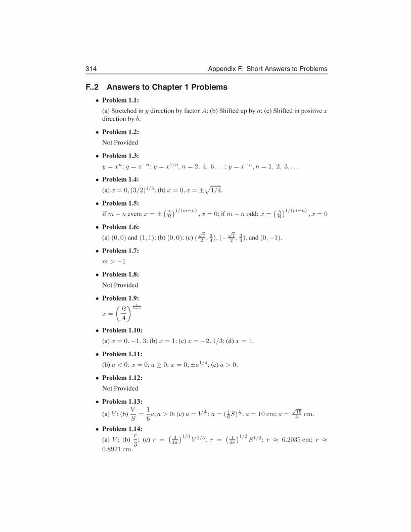
314 Appendix F. Short Answers to Problems
F..2 Answers to Chapter 1 Problems• Problem 1.1:
(a) Stretched in y direction by factor A; (b) Shifted up by a; (c) Shifted in positive xdirection by b.
• Problem 1.2:Not Provided
• Problem 1.3:y = xn; y = x−n; y = x1/n, n = 2, 4, 6, . . .; y = x−n, n = 1, 2, 3, . . .
• Problem 1.4:(a) x = 0, (3/2)1/3; (b) x = 0, x = ±
√
1/4.
• Problem 1.5:if m− n even: x = ±
(
AB
)1/(m−n), x = 0; if m− n odd: x =
(
AB
)1/(m−n), x = 0
• Problem 1.6:(a) (0, 0) and (1, 1); (b) (0, 0); (c) (
√72 , 3
4 ), (−√72 , 3
4 ), and (0,−1).
• Problem 1.7:m > −1
• Problem 1.8:Not Provided
• Problem 1.9:
x =
(
B
A
)1
b−a
• Problem 1.10:(a) x = 0, −1, 3; (b) x = 1; (c) x = −2, 1/3; (d) x = 1.
• Problem 1.11:(b) a < 0: x = 0; a ≥ 0: x = 0, ±a1/4; (c) a > 0.
• Problem 1.12:Not Provided
• Problem 1.13:
(a) V ; (b) VS
=1
6a, a > 0; (c) a = V
13 ; a = (16S)
12 ; a = 10 cm; a =
√153 cm.
• Problem 1.14:(a) V ; (b) r
3; (c) r =
(
34π
)1/3V 1/3; r =
(
14π
)1/2S1/2; r ≈ 6.2035 cm; r ≈
0.8921 cm.

315
• Problem 1.15:r = 2k1/k2 = 12µm.
• Problem 1.16:(a) P = C
(
RA
)d/b; (b) S = 4π(
3V4π
)2/3.
• Problem 1.17:(a) a: Ms−1, b: s−1; (b) b = 0.2, a = 0.002; (c) v = 0.001.
• Problem 1.18:(a) v ≈ K , (b) v = K/2.
• Problem 1.19:K ≈ 0.0048, kn ≈ 77 nM
• Problem 1.20:(a) x = −1, 0, 1 (b) 1 (c) y1 (d) y2.
• Problem 1.21:Line of slope a3/A and intercept 1/A
• Problem 1.22:K = 0.5, a = 2
• Problem 1.23:Not Provided
• Problem 1.24:m ≈ 67, b ≈ 1.2, K ≈ 0.8, kn ≈ 56
• Problem 1.25:
x =(
RA
)1
r−a
316 Appendix F. Short Answers to Problems
F..3 Answers to Chapter 2 Problems• Problem 2.1:
(a) m = 28◦/min, b = 50.
• Problem 2.2:(a) −4.91◦F/min. (b) -7, -8, -9 ◦F/min. (c) -9 ◦F/min.
• Problem 2.3:Displacements have same magnitude, opposite signs.
• Problem 2.4:(b) 9.8 m/s.
• Problem 2.5:(a) −14.7 m/s; (b) −gt− gε
2 ; (c) t = 10 s.
• Problem 2.6:v0 − g/2
• Problem 2.7:v̄ = 13.23 m/s.; secant line is y = 13.23x− 2.226
• Problem 2.8:(a) 2; (b) 0; (c) −2; (d) 0.
• Problem 2.9:(a) 1; 1; 1; (b) 1; 0; 1; (c) 1; 2; 4.
• Problem 2.10:(a) 3; (b) 5.55; (c) 32
3 .
• Problem 2.11:(a) 2
√2
π ; (b) 6(1−√2)
π ; (c) π/4 ≤ x ≤ 5π/4 (one solution).
• Problem 2.12:(a) 2 + h; (b) 2; (c) y = 2x.
• Problem 2.13:2h2 + 25h+ 104; 104
• Problem 2.14:(b) 0,−4,−1.9,−2.1,−2− h; (c) −2.
• Problem 2.15:(a) 2 + h; (b) 2; (c) 2.98.
317
• Problem 2.16:(a) 4
π ; (b) 4√3−12π .
• Problem 2.17:(a) −1; (b) −2
1+ε ; (c) Slope approaches -2; (d) y = −2x+ 4.
• Problem 2.18:(a) v(2) = 12 m/s; v̄ = 15 m/s; (b) v(2) = 0 m/s; v̄ = 25 m/s; (c) v(2) = 13 m/s;v̄ = 11 m/s.
• Problem 2.19:0
• Problem 2.20:−1
(x+1)2
318 Appendix F. Short Answers to Problems
F..4 Answers to Chapter 3 Problems• Problem 3.1:
Not Provided
• Problem 3.2:Not Provided
• Problem 3.3:5; 5; no change; linear function
• Problem 3.4:(a) no tangent line; (b) y = −(x+ 1); (c) y = (x+ 1).
• Problem 3.5:(a) increasing: −∞ < x < 0, 1.5 < x < ∞; decreasing for 0 < x < 1.5; (b) 0,local maximum; 1.5, local minimum; (c) No.
• Problem 3.6:Not Provided
• Problem 3.7:Not Provided
• Problem 3.8:Not Provided
• Problem 3.9:y = 2x− 3
• Problem 3.10:Not Provided
• Problem 3.11:(a) f ′(x) = 2x, f ′(0) = 0, f ′(1) = 2 > 0, f ′(−1) = −2 < 0. Local minimum atx = 0; (b) f ′(x) = −3x2, f ′(0) = 0, f ′(1) = −3 < 0, f ′(−1) = −3 < 0. No localmaxima nor minima; (c) f ′(x) = −4x3, f ′(0) = 0, f ′(1) = −4 < 0,f ′(−1) = 4 >0. Local maximum at x = 0.
• Problem 3.12:Not Provided
• Problem 3.13:Not Provided
• Problem 3.14:Not Provided
319
• Problem 3.15:5
• Problem 3.16:(a) y = 3x− 2; (b) x = 2/3; (c) 1.331; 1.3.
• Problem 3.17:(a) y = −4x+ 5; (b) x = 5/4, y = 5; (c) y = 0.6, smaller.
• Problem 3.18:
(a) y = f ′(x0)(x− x0) + f(x0); (b) x = x0 −f(x0)
f ′(x0).
• Problem 3.19:Not Provided
• Problem 3.20:Not Provided
• Problem 3.21:(a) 14.7 m/s; (b) −4.9 m/s.
• Problem 3.22:(b) a = 2.
• Problem 3.23:(3, 9), (1, 1)
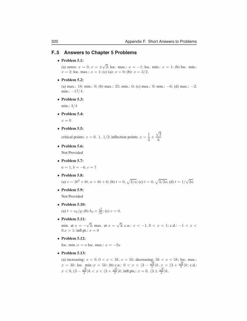
320 Appendix F. Short Answers to Problems
F..5 Answers to Chapter 5 Problems• Problem 5.1:
(a) zeros: x = 0, x = ±√3; loc. max.: x = −1; loc. min.: x = 1; (b) loc. min.:
x = 2; loc. max.: x = 1; (c) (a): x = 0; (b): x = 3/2.
• Problem 5.2:(a) max.: 18; min.: 0; (b) max.: 25; min.: 0; (c) max.: 0; min.: −6; (d) max.: −2;min.: −17/4.
• Problem 5.3:min.: 3/4
• Problem 5.4:x = 0
• Problem 5.5:
critical points: x = 0, 1, 1/2; inflection points: x =1
2±
√3
6
• Problem 5.6:Not Provided
• Problem 5.7:a = 1, b = −6, c = 7
• Problem 5.8:(a) v = 3t2 + 6t, a = 6t+ 6; (b) t = 0,
√
3/a; (c) t = 0,√
3/2a; (d) t = 1/√2a.
• Problem 5.9:Not Provided
• Problem 5.10:(a) t = v0/g; (b) h0 +
v20
2g ; (c) v = 0.
• Problem 5.11:min. at x = −
√3; max. at x =
√3; c.u.: x < −1, 0 < x < 1; c.d.: −1 < x <
0,x > 1; infl.pt.: x = 0
• Problem 5.12:loc. min.:x = a loc. max.: x = −2a
• Problem 5.13:(a) increasing: x < 0, 0 < x < 3k, x > 5k; decreasing: 3k < x < 5k; loc. max.:x = 3k; loc. min.:x = 5k; (b) c.u.: 0 < x < (3 −
√62 )k, x > (3 +
√62 )k; c.d.:
x < 0, (3 −√62 )k < x < (3 +
√62 )k; infl.pts.: x = 0, (3±
√62 )k.
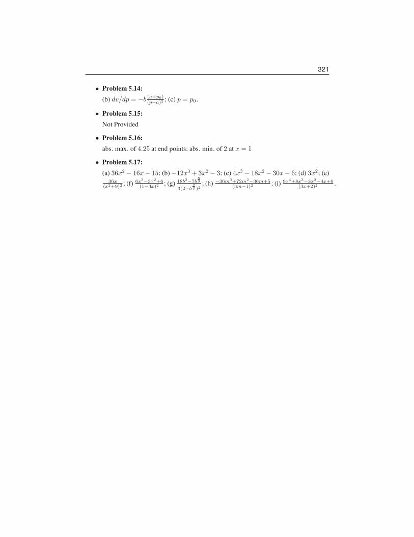
321
• Problem 5.14:(b) dv/dp = −b (a+p0)
(p+a)2 ; (c) p = p0.
• Problem 5.15:Not Provided
• Problem 5.16:abs. max. of 4.25 at end points; abs. min. of 2 at x = 1
• Problem 5.17:(a) 36x2 − 16x− 15; (b) −12x3 + 3x2 − 3; (c) 4x3 − 18x2 − 30x− 6; (d) 3x2; (e)
36x(x2+9)2 ; (f) 6x3−3x2+6
(1−3x)2 ; (g) 18b2−7b83
3(2−b23 )2
; (h) −36m3+72m2−36m+5(3m−1)2 ; (i) 9x4+8x3−3x2−4x+6
(3x+2)2 .
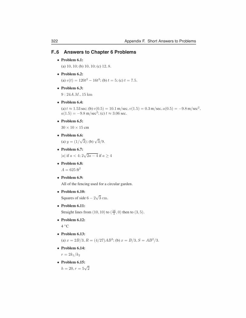
322 Appendix F. Short Answers to Problems
F..6 Answers to Chapter 6 Problems• Problem 6.1:
(a) 10, 10; (b) 10, 10; (c) 12, 8.
• Problem 6.2:(a) v(t) = 120t2 − 16t3; (b) t = 5; (c) t = 7.5.
• Problem 6.3:9 : 24A.M., 15 km
• Problem 6.4:(a) t ≈ 1.53 sec; (b) v(0.5) = 10.1m/sec, v(1.5) = 0.3m/sec, a(0.5) = −9.8m/sec2,a(1.5) = −9.8 m/sec2; (c) t ≈ 3.06 sec.
• Problem 6.5:30× 10× 15 cm
• Problem 6.6:(a) y = (1/
√3); (b)
√3/9.
• Problem 6.7:|a| if a < 4; 2
√2a− 4 if a ≥ 4
• Problem 6.8:A = 625 ft2
• Problem 6.9:All of the fencing used for a circular garden.
• Problem 6.10:Squares of side 6− 2
√3 cm.
• Problem 6.11:Straight lines from (10, 10) to (163 , 0) then to (3, 5).
• Problem 6.12:4 ◦C
• Problem 6.13:(a) x = 2B/3, R = (4/27)AB3; (b) x = B/3, S = AB2/3.
• Problem 6.14:r = 2k1/k2
• Problem 6.15:h = 20, r = 5
√2
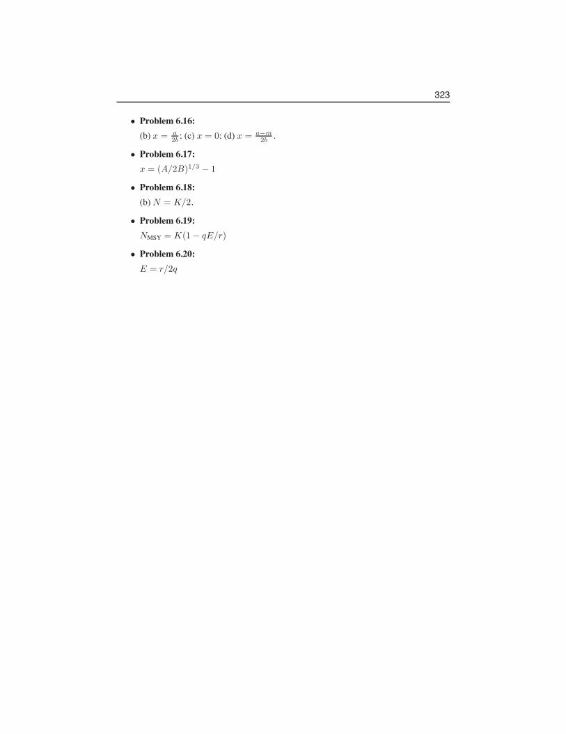
323
• Problem 6.16:(b) x = a
2b ; (c) x = 0; (d) x = a−m2b .
• Problem 6.17:x = (A/2B)1/3 − 1
• Problem 6.18:(b) N = K/2.
• Problem 6.19:NMSY = K(1− qE/r)
• Problem 6.20:E = r/2q
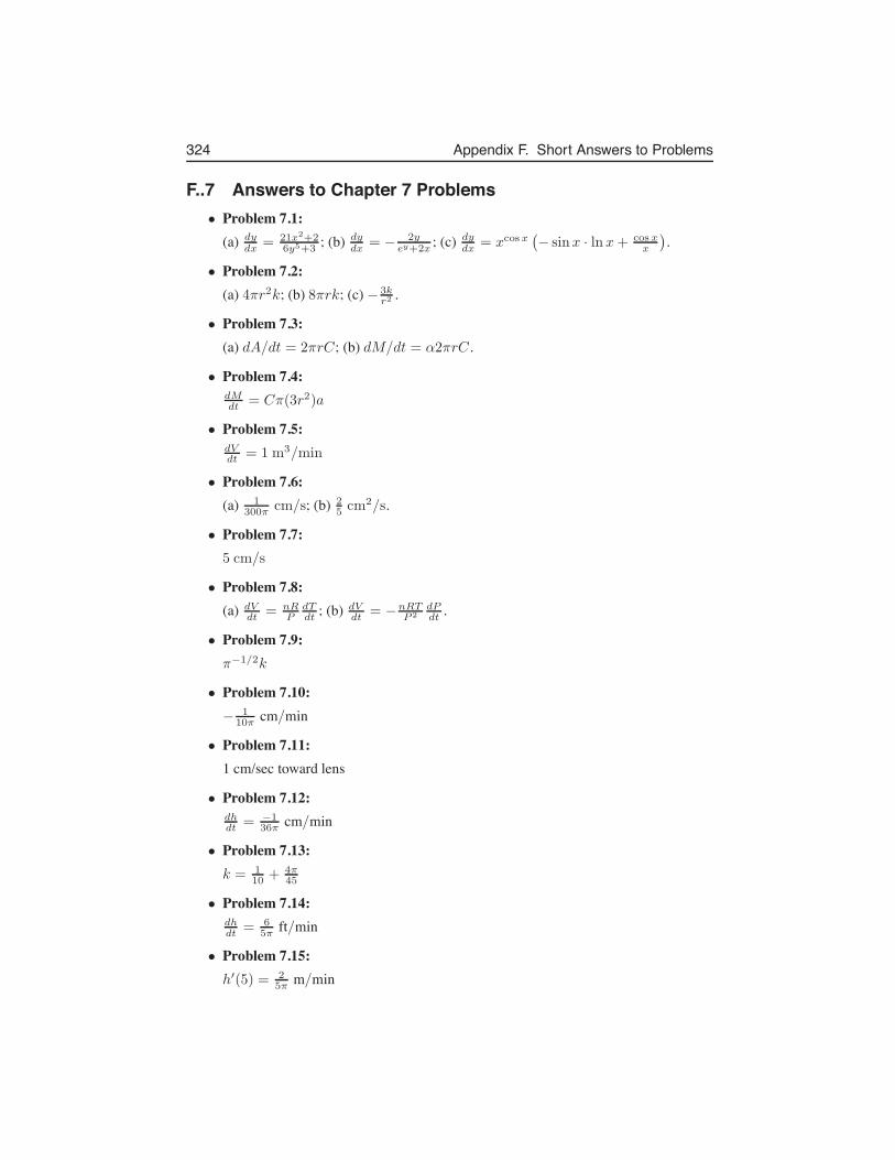
324 Appendix F. Short Answers to Problems
F..7 Answers to Chapter 7 Problems• Problem 7.1:
(a) dydx = 21x2+2
6y5+3 ; (b) dydx = − 2y
ey+2x ; (c) dydx = xcosx
(
− sinx · lnx+ cos xx
)
.
• Problem 7.2:(a) 4πr2k; (b) 8πrk; (c) − 3k
r2 .
• Problem 7.3:(a) dA/dt = 2πrC; (b) dM/dt = α2πrC.
• Problem 7.4:dMdt = Cπ(3r2)a
• Problem 7.5:dVdt = 1 m3/min
• Problem 7.6:(a) 1
300π cm/s; (b) 25 cm2/s.
• Problem 7.7:5 cm/s
• Problem 7.8:(a) dV
dt = nRP
dTdt ; (b) dV
dt = −nRTP 2
dPdt .
• Problem 7.9:π−1/2k
• Problem 7.10:− 1
10π cm/min
• Problem 7.11:1 cm/sec toward lens
• Problem 7.12:dhdt = −1
36π cm/min
• Problem 7.13:k = 1
10 + 4π45
• Problem 7.14:dhdt = 6
5π ft/min
• Problem 7.15:h′(5) = 2
5π m/min
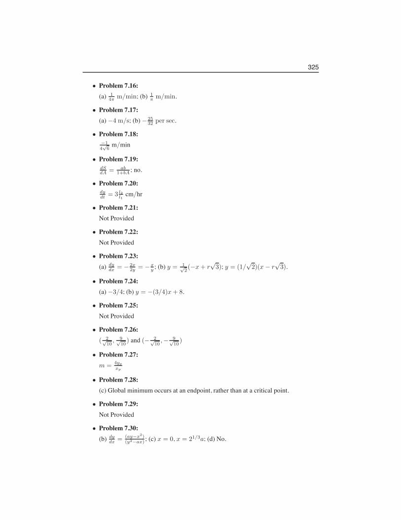
325
• Problem 7.16:(a) 1
4π m/min; (b) 1π m/min.
• Problem 7.17:(a) −4 m/s; (b) − 25
32 per sec.
• Problem 7.18:−14√6
m/min
• Problem 7.19:dSdA = ab
1+bA ; no.
• Problem 7.20:dydt = 3 l2
l1cm/hr
• Problem 7.21:Not Provided
• Problem 7.22:Not Provided
• Problem 7.23:(a) dy
dx = − 2x2y = −x
y ; (b) y = 1√2(−x+ r
√3); y = (1/
√2)(x − r
√3).
• Problem 7.24:(a) −3/4; (b) y = −(3/4)x+ 8.
• Problem 7.25:Not Provided
• Problem 7.26:( 2√
10, 9√
10) and (− 2√
10,− 9√
10)
• Problem 7.27:m = 4yp
xp
• Problem 7.28:(c) Global minimum occurs at an endpoint, rather than at a critical point.
• Problem 7.29:Not Provided
• Problem 7.30:(b) dy
dx = (ay−x2)(y2−ax) ; (c) x = 0, x = 21/3a; (d) No.
326 Appendix F. Short Answers to Problems
• Problem 7.31:(a) dp
dv = (2 av3 )− (p+ a
v2 )/(v − b).
• Problem 7.32:(0, 5/4)
• Problem 7.33:(a) y − 1 = −1(x− 1); (b) y′′ = 4
5 ; (c) concave up.
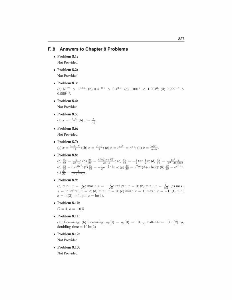
327
F..8 Answers to Chapter 8 Problems• Problem 8.1:
Not Provided
• Problem 8.2:Not Provided
• Problem 8.3:(a) 50.75 > 50.65; (b) 0.4−0.2 > 0.40.2; (c) 1.0012 < 1.0013; (d) 0.9991.5 >0.9992.3.
• Problem 8.4:Not Provided
• Problem 8.5:(a) x = a2b3; (b) x = b
c23
.
• Problem 8.6:Not Provided
• Problem 8.7:(a) x = 3−ln(5)
2 ; (b) x = e4+13 ; (c) x = e(e
2) = ee·e; (d) x = ln(C)a−b .
• Problem 8.8:(a) dy
dx = 62x+3 ; (b) dy
dx = 6[ln(2x+3)]2
2x+3 ; (c) dydx = − 1
2 tan12x; (d) dy
dx = 3x2−2(x3−2x) ln a ;
(e) dydx = 6xe3x
2 ; (f) dydx = − 1
2a− 1
2x ln a; (g) dy
dx = x22x(3+x ln 2); (h) dydx = ee
x+x;(i) dy
dx = 4(et+e−t)2 .
• Problem 8.9:(a) min.: x = 2√
3; max.: x = − 2√
3; infl.pt.: x = 0; (b) min.: x = 1
3√3
; (c) max.:x = 1; inf.pt.: x = 2; (d) min.: x = 0; (e) min.: x = 1; max.: x = −1; (f) min.:x = ln(2); infl. pt.: x = ln(4).
• Problem 8.10:C = 4, k = −0.5
• Problem 8.11:(a) decreasing; (b) increasing; y1(0) = y2(0) = 10; y1 half-life = 10 ln(2); y2doubling-time = 10 ln(2)
• Problem 8.12:Not Provided
• Problem 8.13:Not Provided
328 Appendix F. Short Answers to Problems
• Problem 8.14:Not Provided
• Problem 8.15:crit.pts.: x = 0, x ≈ ±1.64; f(0) = 1; f(±1.64) ≈ −0.272
• Problem 8.16:x = 1/β
• Problem 8.17:(a) x = r; (c) x = ar
a−r ln(
RA
)
; (d) decrease; (e) decrease.
• Problem 8.18:x = b
√
ln((a2 + b2)/b2)
• Problem 8.19:Not Provided
329
F..9 Answers to Chapter 9 Problems• Problem 9.1:
Not Provided
• Problem 9.2:(a) C any value, k = −5; (b) C any value, k = 3.
• Problem 9.3:(a) y(t) = Ce−t; (b) c(x) = 20e−0.1x; (c) z(t) = 5e3t.
• Problem 9.4:t = − ln 2
ln 7−ln 10
• Problem 9.5:(a) 57300 years; (b) 22920 years
• Problem 9.6:(a) 29 years; (b) 58 years; (c) 279.7 years.
• Problem 9.7:(a) 80.7%; (b) 12.3 years.
• Problem 9.8:y ≈ 707.8 torr
• Problem 9.9:(a) P (5) ≈ 1419; (b) t ≈ 9.9years.
• Problem 9.10:dNdt = 0.05N ; N(0) = 250; N(t) = 250e0.05t; 2.1× 10¹⁰ rodents
• Problem 9.11:(a) dy/dt = 2.57y; (b) dy/dt = −6.93y.
• Problem 9.12:(a) 12990; (b) 30792 bacteria.
• Problem 9.13:1.39 hours; 9.2 hours
• Problem 9.14:20 min; 66.44 min
• Problem 9.15:(a) y1 growing, y2 decreasing; (b) 3.5, 2.3; (c) y1(t) = 100e0.2t, y2(t) = 10000e−0.3t;(d) t ≈ 9.2 years.
330 Appendix F. Short Answers to Problems
• Problem 9.16:12265 people/km2
• Problem 9.17:(a) 1 hour; (b) r = ln(2); (c) 0.25 M; (d) t = 3.322 hours.
• Problem 9.18:6.93 years
• Problem 9.19:1.7043 kg
• Problem 9.20:(a) $510, $520.20, $742.97; 17.5 years; for 8% interest: $520, $540.80, $1095.56;(b) $510.08, $520.37, $745.42; (c) 5%.
331
F..10 Answers to Chapter 10 Problems• Problem 10.1:
(a) dydx = 2x cosx2; (b) dy
dx = sin 2x; (c) dydx = − 2
3x− 2
3 (cot 3√x)(csc2 3
√x); (d)
dydx = (1−6x) sec(x−3x2) tan(x−3x2); (e) dy
dx = 6x2 tanx+2x3 sec2 x; (f) dydx =
cosx+x sin xcos2 x ; (g) dy
dx = cosx − x sinx; (h) dydx =
sin 2x
x2esin2 1
x
; (i) dydx = 6(2 tan 3x +
3 cosx)(2 sec2 3x− sinx); (j) dydx = − sin(sinx) · cosx+ cos 2x.
• Problem 10.2:
(a) f ′(x) = −(4x3+10x) sin(ln(x4+5x2+3))(x4+5x2+3) ; (b) f ′(x) =
(3x2−2 cos(x) sin(x)) cos(√
cos2(x)+x3)
(2√
cos2(x)+x3);
(c) f ′(x) = 6x2+ 1x ln(3) ; (d) f ′(x) = 4(x2ex+tan(3x))3(2xex+x2ex+3 sec2(3x));
(e) f ′(x) = 2x√
sin3(x) + cos3(x) + 3x2(sin2(x) cos(x)−cos2(x) sin(x))
2√
sin3(x)+cos3(x).
• Problem 10.3:(a) 180o (b) 300o (c) 164.35o (d) 4320o
(e) 5π/9 (f) 2π/45 (g) 5π/2 (h) π/2
(i) 1/2 (j)√2/2 (k)
√3/3
• Problem 10.4:Not Provided
• Problem 10.5:Not Provided
• Problem 10.6:Not Provided
• Problem 10.7:−√3/20, 1/20
• Problem 10.8:(a) [0,π/4], [5π/4, 2π]; (b) [3π/4, 7π/4]; (c) x = 3π/4, 7π/4.
• Problem 10.9:(a) T (t) = 37.1 + 0.4 cos[π(t− 8)/12]; (b) W (t) = 0.5 + 0.5 cos[π(t− 8)/6].
• Problem 10.10:(a) S = 3 cos
(√ gl t)
; (b) y = 2 sin(
2π3 t+ π
6
)
+ 10.
• Problem 10.11:±(π8 , 1)
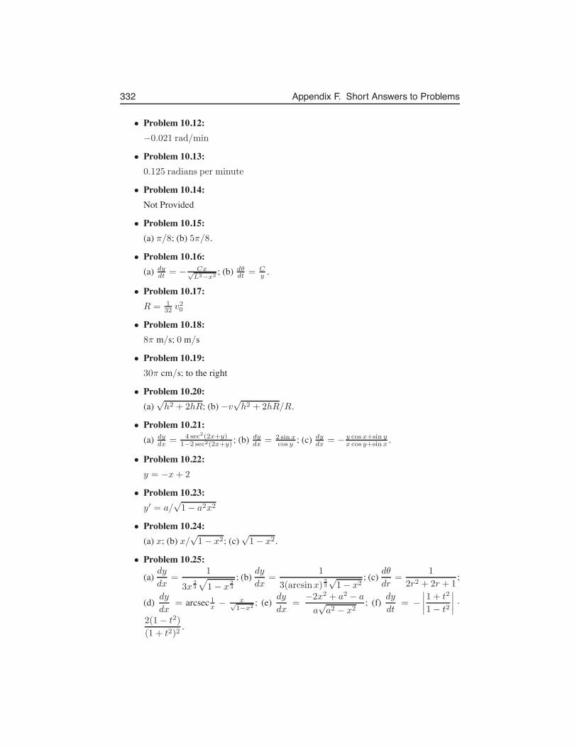
332 Appendix F. Short Answers to Problems
• Problem 10.12:−0.021 rad/min
• Problem 10.13:0.125 radians per minute
• Problem 10.14:Not Provided
• Problem 10.15:(a) π/8; (b) 5π/8.
• Problem 10.16:(a) dy
dt = − Cx√L2−x2
; (b) dθdt = C
y .
• Problem 10.17:R = 1
32 v20
• Problem 10.18:8π m/s; 0 m/s
• Problem 10.19:30π cm/s; to the right
• Problem 10.20:(a)
√h2 + 2hR; (b) −v
√h2 + 2hR/R.
• Problem 10.21:(a) dy
dx = 4 sec2(2x+y)1−2 sec2(2x+y) ; (b) dy
dx = 2 sin xcos y ; (c) dy
dx = − y cosx+sin yx cos y+sin x .
• Problem 10.22:y = −x+ 2
• Problem 10.23:y′ = a/
√1− a2x2
• Problem 10.24:(a) x; (b) x/
√1− x2; (c)
√1− x2.
• Problem 10.25:
(a)dy
dx=
1
3x23
√
1− x23
; (b)dy
dx=
1
3(arcsinx)23
√1− x2
; (c)dθ
dr=
1
2r2 + 2r + 1;
(d) dy
dx= arcsec 1
x − x√1−x2
; (e) dy
dx=
−2x2 + a2 − a
a√a2 − x2
; (f) dy
dt= −
∣
∣
∣
∣
1 + t2
1− t2
∣
∣
∣
∣
·
2(1− t2)
(1 + t2)2.
333
• Problem 10.26:0.4 m
• Problem 10.27:526 rad/s
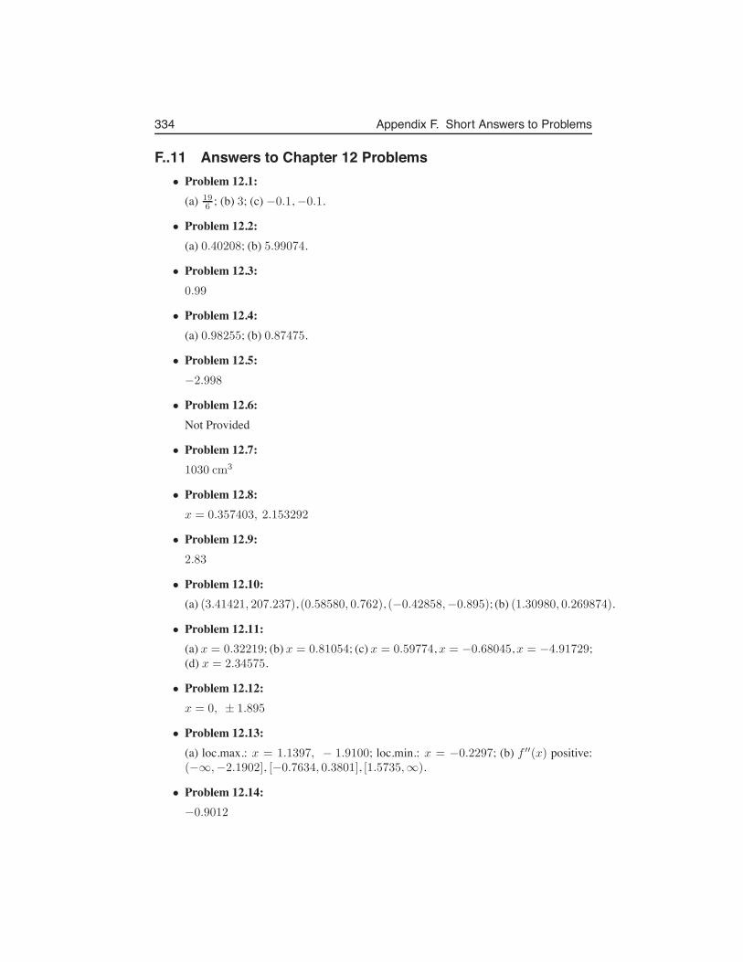
334 Appendix F. Short Answers to Problems
F..11 Answers to Chapter 12 Problems• Problem 12.1:
(a) 196 ; (b) 3; (c) −0.1, −0.1.
• Problem 12.2:(a) 0.40208; (b) 5.99074.
• Problem 12.3:0.99
• Problem 12.4:(a) 0.98255; (b) 0.87475.
• Problem 12.5:−2.998
• Problem 12.6:Not Provided
• Problem 12.7:1030 cm3
• Problem 12.8:x = 0.357403, 2.153292
• Problem 12.9:2.83
• Problem 12.10:(a) (3.41421, 207.237), (0.58580, 0.762), (−0.42858,−0.895); (b) (1.30980, 0.269874).
• Problem 12.11:(a) x = 0.32219; (b) x = 0.81054; (c) x = 0.59774, x = −0.68045, x = −4.91729;(d) x = 2.34575.
• Problem 12.12:x = 0, ± 1.895
• Problem 12.13:(a) loc.max.: x = 1.1397, − 1.9100; loc.min.: x = −0.2297; (b) f ′′(x) positive:(−∞,−2.1902], [−0.7634, 0.3801], [1.5735,∞).
• Problem 12.14:−0.9012
335
• Problem 12.15:Not Provided
• Problem 12.16:(a) y5 = 1.61051; y(0.5) = 1.6487213; error = 0.03821; (b) y5 = 0.59049;y(0.5) = 0.60653; error = 0.01604.
• Problem 12.17:0.55, 0.5995, 0.6475, 0.6932, 0.7357
• Problem 12.18:Not Provided
• Problem 12.19:(a) 0.806; (b) 0.681; (c) 4.027.
• Problem 12.20:(a) 1.112; (b) 0.622.
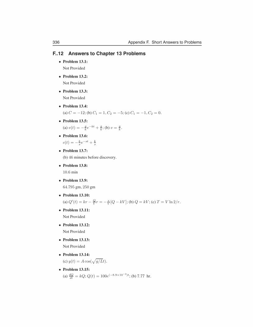
336 Appendix F. Short Answers to Problems
F..12 Answers to Chapter 13 Problems• Problem 13.1:
Not Provided
• Problem 13.2:Not Provided
• Problem 13.3:Not Provided
• Problem 13.4:(a) C = −12; (b) C1 = 1, C2 = −5; (c) C1 = −1, C2 = 0.
• Problem 13.5:(a) v(t) = − g
k e−kt + g
k ; (b) v = gk .
• Problem 13.6:c(t) = −k
s e−st + k
s
• Problem 13.7:(b) 46 minutes before discovery.
• Problem 13.8:10.6 min
• Problem 13.9:64.795 gm, 250 gm
• Problem 13.10:(a) Q′(t) = kr − Q
V r = − rV [Q− kV ]; (b) Q = kV ; (c) T = V ln 2/r.
• Problem 13.11:Not Provided
• Problem 13.12:Not Provided
• Problem 13.13:Not Provided
• Problem 13.14:(c) y(t) = A cos(
√
g/Lt).
• Problem 13.15:(a) dQ
dt = kQ; Q(t) = 100e(−8.9×10⁻²)t; (b) 7.77 hr.
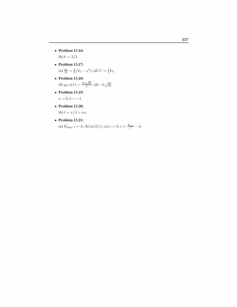
337
• Problem 13.16:(b) k = 3/2.
• Problem 13.17:(a) dx
dt = k3 (V0 − x3); (d) V = 1
2V0.
• Problem 13.18:(b) y0; (c) t = 2A
√y0
k ; (d) −k√y0.
• Problem 13.19:a = 0, b = −1
• Problem 13.20:(b) t = π/4 + nπ.
• Problem 13.21:(a) Kmax, c = k; (b) ln(2)/r; (c) c = 0, c = Kmax
r − k.
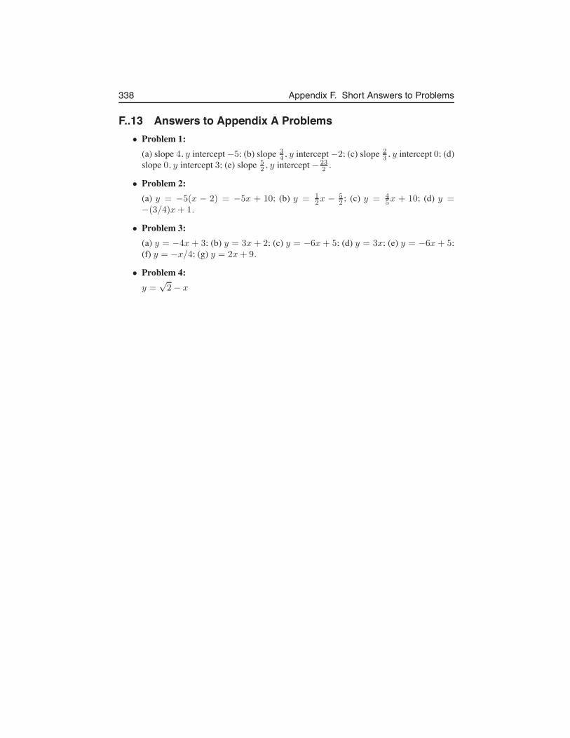
338 Appendix F. Short Answers to Problems
F..13 Answers to Appendix A Problems• Problem 1:
(a) slope 4, y intercept −5; (b) slope 34 , y intercept −2; (c) slope 2
3 , y intercept 0; (d)slope 0, y intercept 3; (e) slope 5
2 , y intercept − 232 .
• Problem 2:(a) y = −5(x − 2) = −5x + 10; (b) y = 1
2x − 52 ; (c) y = 4
5x + 10; (d) y =−(3/4)x+ 1.
• Problem 3:(a) y = −4x+ 3; (b) y = 3x+ 2; (c) y = −6x+ 5; (d) y = 3x; (e) y = −6x+ 5;(f) y = −x/4; (g) y = 2x+ 9.
• Problem 4:y =
√2− x
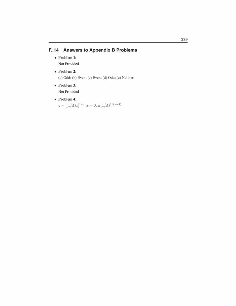
339
F..14 Answers to Appendix B Problems• Problem 1:
Not Provided
• Problem 2:(a) Odd; (b) Even; (c) Even; (d) Odd; (e) Neither.
• Problem 3:Not Provided
• Problem 4:y = [(1/A)x]1/n; x = 0,±(1/A)1/(n−1)

340 Appendix F. Short Answers to Problems
Index
Arrhenius, 161differential equation, 169Lysteria
monocytogenes, 70power function, 2
acceleration, 63, 67uniform, 64
ActA, 70actin, 70age distribution, 173
uniform, 173airplane, 87allometric constants, 160allometry, 159ambient temperature, 180, 252amplitude, 194Andromeda strain, 149, 158angle
degrees, 189radians, 190
ant trails, 137antiderivative, 62antidifferentiation, 62, 64approximation
linear, 227arc length, 190arccosine, 212arcsine, 210arctan, 214argument
geometric, 5astroid, 130attention, 133attraction, 13average
rate of change, 27, 29
baseof exponent, 149
biochemicalreaction, 9
bird flock, 13birth rate
human, 174box
rectangular, 100
carrying capacity, 95, 264cell
length, 100shape, 1size, 97spherical, 2
cesium-137, 179chain rule, 119Chernoby, 179circle
area of, 189clock hands, 202, 203coffee budget, 121comet tail, 70concave
down, 78up, 78
cone, 124constraint, 99converge, 234, 237cooling, 23cooling object, 257cosine, 308
derivative, 199Crichton
Michael, 149critical point, 79, 231, 234
341
342 Index
critical pointsclassifying, 85
cryptic food, 133cubic, 59cycle
peridic, 194cylinder
surface area, 98volume, 98
daylight cycle, 195decay
exponential, 178decreasing
function, 78degree
of polynomial, 61density dependent
growth, 95growth rate, 264
derivative, 34, 40definition, 34
differential equation, 155, 156, 167, 217,241, 249
DillLarry, 205
displacement, 25, 27doubling time, 176, 177Dukas
Reuven, 133
E. coli, 149ellipse
rotated, 131endpoints
maxima at, 102energy gain, 109enzyme, 9equinox, 196Euler’s method, 183, 227, 238, 250, 266even
function, 3, 4, 6, 193exponential decay, 250exponential function, 152, 167
base 10, 153base 2, 153
base e, 154exponential growth, 239, 250
falling object, 27, 63, 65, 255fertility, 173fish school, 13food patch, 108food type, 133foraging
optimal, 108frequency, 194
Galileo, 31geometric argument, 5, 111geometric relationships, 122gravity, 31, 63growth rate, 174
intrinsic, 95
half life, 178harmonic oscillator, 217heating, 23Hill
coefficient, 12function, 11
hormone cycle, 196
identitytrigonometric, 192
implicit differentiation, 125, 217increasing
function, 78inflection
point, 78infusion, 256initial
velocity, 64initial guess, 236initial value, 170
problem, 238instantaneous
rate of change, 34intrinsic growth rate, 264inverse function, 156, 210iodine-131, 179iteration, 233
Index 343
iteration scheme, 227
Kepler, 103wedding, 103
Lactobacillus, 23landing system, 87law of cosines, 201, 308level curves, 217linear, 24
approximation, 227, 228operation, 61
linearityof derivative, 61of limits, 300
Linweaver-Burke, 14local
maximum, 79minimum, 79
log-log plot, 159logarithm
natural, 156logistic
growth, 95logistic equation, 263, 264logistic growth, 95
maximum, 95absolute, 87global, 87
Michaelis-Mentenkinetics, 10
milktemperature, 23
minimum, 95absolute, 87global, 87local, 6
modelmathematical, 1
molecular collision, 161moon phase, 197mortality, 174moving bead, 70moving object, 25murder mystery, 254
net growth rate, 172Newton’s
law of cooling, 180, 241, 252method, 5, 227, 230
nMnano Molar, 11
nonlinear, 25differential equation, 263
nuclear power plant, 179numerical solution, 183nutrient
absorption, 3balance, 2consumption, 3
oddfunction, 3, 4, 6, 193
one-to-one, 7, 210oxygen, 6
parameter, 171per capita
birth rate, 171mortality rate, 171
percentgrowth, 174
perimetermaximal, 102of circle, 190
period, 192periodic function, 192phase shift, 195pheromone, 137pollution, 120polynomial, 7, 61
degree, 7derivative of, 61
populationdensity, 95growth, 171, 249
position, 67power
dominant, 3function, 3, 4, 59
power rule, 59, 86, 128powers
344 Index
of 2, 150predator
size, 206Preface, xviiproportional, 2proportionality
constant, 2Pythagoras theorem, 107, 210, 212
race track, 201radian, 41, 190radioactive decay, 177radioactivity, 177rate
constant, 174rate of change
average, 23, 27, 29instantaneous, 59
rate of increasenet, 96
rational function, 9, 10reaction
speed, 10related rates, 200repulsion, 13rescaling, 265residence time, 110restricting the domain, 210roots, 230
of equation, 237
saturation, 11scientific problems, 171secant line, 28, 29, 31second derivative, 62, 80second order
DE, 217shortest path, 137sine, 308
derivative, 199sketching
the derivative, 44, 67slope
of tangent line, 40, 59slope field, 259solution
approximate, 227numerical, 227to differential equation, 169
solution curve, 249, 253spacing distance, 13spreadsheet, 234, 240stability, 263stable
steady state, 263steady state, 261step size, 239stroboscope, 25substrate, 9superposition, 7symmetry, 3
tangentto a circle, 45
tangent line, 34, 40, 42, 62, 72temperature
ambient, 180, 241milk, 23
terminal velocity, 255time of death, 254trigonometric functions, 189, 210trigonometric identities, 308tumor growth, 122
unbounded, 6unit circle, 190unstable, 263
velocity, 25, 63, 67average, 25instantaneous, 25, 32
visual angle, 204, 216
wine barrel, 103
yoghurt, 23
zebra danio, 206zeros
of a function, 45, 83, 230zoom, 40