Differentiable Direct Volume Rendering

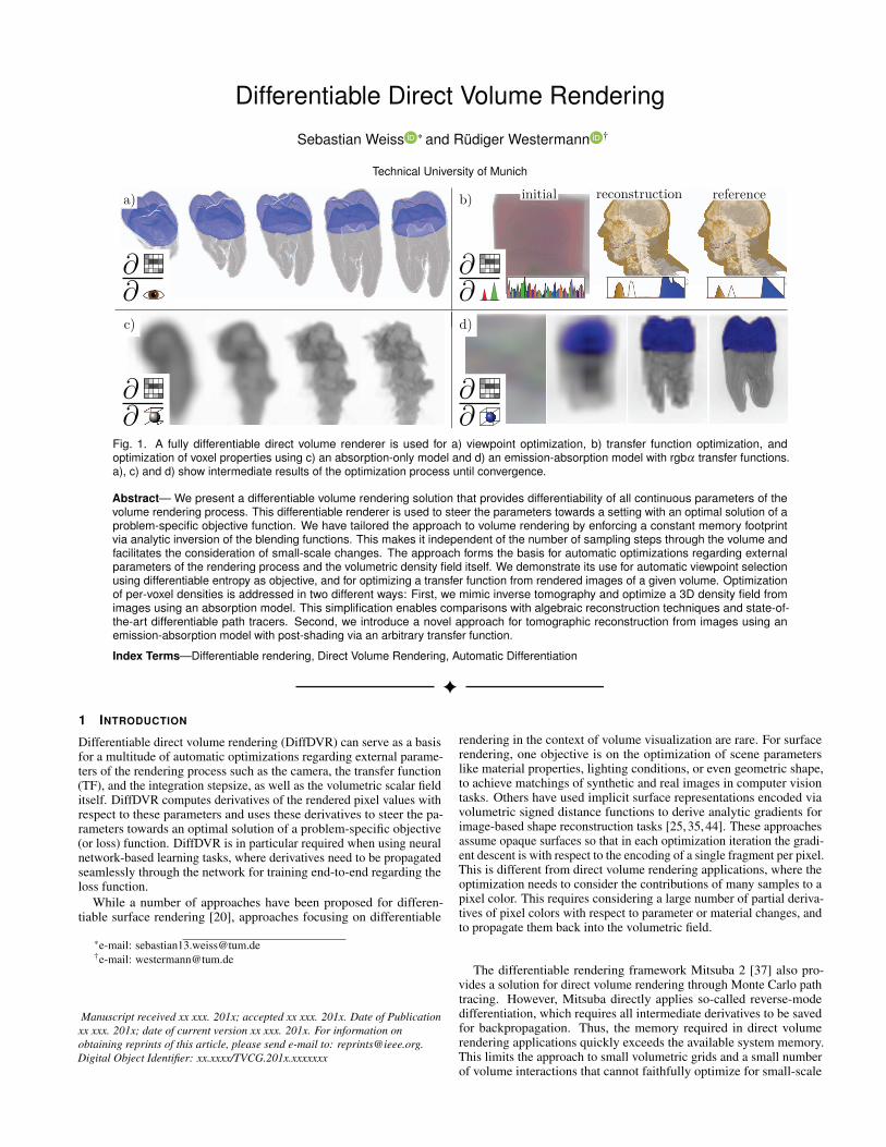
Differentiable Direct Volume Rendering

Sebastian Weiss * and Rudiger Westermann †

Technical University of Munich

∂∂

∂∂

∂∂

∂∂

Fig. 1. A fully differentiable direct volume renderer is used for a) viewpoint optimization, b) transfer function optimization, andoptimization of voxel properties using c) an absorption-only model and d) an emission-absorption model with rgbα transfer functions.a), c) and d) show intermediate results of the optimization process until convergence.

Abstract— We present a differentiable volume rendering solution that provides differentiability of all continuous parameters of thevolume rendering process. This differentiable renderer is used to steer the parameters towards a setting with an optimal solution of aproblem-specific objective function. We have tailored the approach to volume rendering by enforcing a constant memory footprintvia analytic inversion of the blending functions. This makes it independent of the number of sampling steps through the volume andfacilitates the consideration of small-scale changes. The approach forms the basis for automatic optimizations regarding externalparameters of the rendering process and the volumetric density field itself. We demonstrate its use for automatic viewpoint selectionusing differentiable entropy as objective, and for optimizing a transfer function from rendered images of a given volume. Optimizationof per-voxel densities is addressed in two different ways: First, we mimic inverse tomography and optimize a 3D density field fromimages using an absorption model. This simplification enables comparisons with algebraic reconstruction techniques and state-of-the-art differentiable path tracers. Second, we introduce a novel approach for tomographic reconstruction from images using anemission-absorption model with post-shading via an arbitrary transfer function.

Index Terms—Differentiable rendering, Direct Volume Rendering, Automatic Differentiation

1 INTRODUCTION

Differentiable direct volume rendering (DiffDVR) can serve as a basisfor a multitude of automatic optimizations regarding external parame-ters of the rendering process such as the camera, the transfer function(TF), and the integration stepsize, as well as the volumetric scalar fielditself. DiffDVR computes derivatives of the rendered pixel values withrespect to these parameters and uses these derivatives to steer the pa-rameters towards an optimal solution of a problem-specific objective(or loss) function. DiffDVR is in particular required when using neuralnetwork-based learning tasks, where derivatives need to be propagatedseamlessly through the network for training end-to-end regarding theloss function.

While a number of approaches have been proposed for differen-tiable surface rendering [20], approaches focusing on differentiable

*e-mail: [email protected]†e-mail: [email protected]

Manuscript received xx xxx. 201x; accepted xx xxx. 201x. Date of Publicationxx xxx. 201x; date of current version xx xxx. 201x. For information onobtaining reprints of this article, please send e-mail to: [email protected] Object Identifier: xx.xxxx/TVCG.201x.xxxxxxx

rendering in the context of volume visualization are rare. For surfacerendering, one objective is on the optimization of scene parameterslike material properties, lighting conditions, or even geometric shape,to achieve matchings of synthetic and real images in computer visiontasks. Others have used implicit surface representations encoded viavolumetric signed distance functions to derive analytic gradients forimage-based shape reconstruction tasks [25, 35, 44]. These approachesassume opaque surfaces so that in each optimization iteration the gradi-ent descent is with respect to the encoding of a single fragment per pixel.This is different from direct volume rendering applications, where theoptimization needs to consider the contributions of many samples to apixel color. This requires considering a large number of partial deriva-tives of pixel colors with respect to parameter or material changes, andto propagate them back into the volumetric field.

The differentiable rendering framework Mitsuba 2 [37] also pro-vides a solution for direct volume rendering through Monte Carlo pathtracing. However, Mitsuba directly applies so-called reverse-modedifferentiation, which requires all intermediate derivatives to be savedfor backpropagation. Thus, the memory required in direct volumerendering applications quickly exceeds the available system memory.This limits the approach to small volumetric grids and a small numberof volume interactions that cannot faithfully optimize for small-scale

structures. A follow-up work [36] addresses this issue but limits thedifferentiability to volume densities and colors.

1.1 ContributionThis work presents a general solution for DiffDVR: differentiable Di-rect Volume Rendering using the emission-absorption model withoutmultiple scattering. This requires analyzing approaches for automaticdifferentiation (AD) with respect to the specific requirements in di-rect volume rendering (DVR). So-called forward-mode approaches areefficient if the number of parameters is low, yet they become com-putationally too expensive with an increasing number of parameters,i.e., when optimizing for per-voxel densities in a volumetric field. Theso-called reverse mode or adjoint mode records the operations and inter-mediate results in a graph structure. This structure is then traversed inreverse order during the backward pass that propagates the changes tothe sample locations. However, this requires storing O(kn) intermediateresults, where n is the number of pixels and k the number of samplelocations, and reversing the order of operations.

We show that a-priori knowledge about the operations performedin DVR can be exploited to avoid recording the operations in reverse-mode AD. We propose a custom computation kernel that inverts theorder of operations in turn and derives the gradients used by AD. Wefurther present a method for recomputing intermediate results via ananalytic inversion of the light accumulation along the view rays. Bythis, intermediate results do not need to be recorded and the memoryconsumption of reverse-mode AD becomes proportional to O(n).

As our second contribution, we discuss a number of use cases inwhich AD is applied in volume rendering applications (Fig. 1). Theseuse cases demonstrate the automatic optimization of external param-eters of the rendering process, i.e., the camera and the TF. Here the3D density field is not changed, but the optimization searches for theexternal parameters that—when used to render this field—yield an opti-mal solution of a problem-specific loss function. In addition, we coverproblems where the optimization is with respect to the densities. I.e.,the field values are optimized so that an image-based loss function—after rendering the optimized field—yields an optimal solution. Weconsider inverse tomography by restricting the rendering process to anabsorption-only model without a TF and optimize the densities usinggiven images of the field. For this case, we compare our method againstalgebraic reconstruction techniques [49, 50] and Mitsuba 2 [36, 37].Beyond that, and for the first time to our best knowledge, we show howto incorporate TFs and an emission-absorption model into tomographicreconstruction and deal with the resulting non-convex optimizationproblem.

DiffDVR is written in C++ and CUDA, and it provides seamlessinteroperability with PyTorch for a simple embedding into existingtraining environments with complex, potentially network-based lossfunctions. The code is made publicly available under a BSD license1.

2 RELATED WORK

Differentiable Rendering A number of differentiable renderershave been introduced for estimating scene parameters or even geometryfrom reference images, for example, under the assumption of localillumination and smooth shading variations [21,26,41,42], or via edgesampling to cope with discontinuities at visibility boundaries [24].Scattering parameters of homogeneous volumes have been estimatedfrom observed scattering pattern [12]. Recently, Nimier-David et al.proposed Mitsuba 2 [37], a fully-differentiable physically-based Monte-Carlo renderer. Mitsuba 2 also handles volumetric objects, yet it re-quires storing intermediate results during the ray sampling process ateach sampling point. This quickly exceeds the available memory andmakes the approach unfeasible for direct volume rendering applications.Later, the authors have shown how to avoid storing the intermediate re-sults [36], by restricting the parameters that can be derived to, e.g., onlyshading and emission. However, these methods are tailored for pathtracing with multiple scattering and rely on Monte-Carlo integrationwith delta tracking. This makes them prone to noise and leads to long

1https://github.com/shamanDevel/DiffDVR

computation times compared to classical DVR methods without scat-tering. Our method, in contrast, does not require storing intermediateresults and can, thus, use large volumes with arbitrary many samplingsteps without resorting to a restricted parameter set. Furthermore, itdoes not impose restrictions on the parameters of the volume renderingprocess that can be differentiated.

Parameter Optimization for Volume Visualization An interest-ing problem in volume visualization is the automatic optimization ofvisualization parameters like the viewpoint, the TF, or the samplingstepsize that is required to convey the relevant information in the mostefficient way. This requires at first hand an image-based loss functionthat can be used to steer the optimizer toward an optimal parametersetting. To measure a viewpoint’s quality from a rendered image,loss functions based on image entropy [7, 19, 46, 51] or image similar-ity [47, 57] have been used. For volume visualization, the relationshipsbetween image entropy and voxel significance [5] as well as importancemeasures of specific features like isosurfaces [45] have been considered.None of these methods, however, considers the rendering process inthe optimization process. Instead, views are first generated from manyviewpoints, e.g., by sampling via the Fibonacci sphere algorithm [28],and then the best view regarding the used loss function is determined.We envision that by considering the volume rendering process in theoptimization, more accurate and faster reconstructions can be achieved.

Another challenging problem is the automatic selection of a “mean-ingful” TF for a given dataset, as the features to be displayed dependhighly on the user expectation. Early works attempted to find a goodTF using clusters in histograms of statistical image properties [15] orfitting visibility histograms [8]. Others have focused on guiding anexplorative user interaction [27, 59], also by using neural networks [3].For optimizing a TF based on information measures, Ruiz et al. [43]proposed to bin voxels of similar density and match their visibility dis-tribution from multiple viewpoints with a target distribution defined bylocal volume features. For optimization, the authors employ a gradient-based method where the visibility derivatives for each density bin areapproximated via local linearization.

Concerning the performance of direct volume rendering, it is crucialto determine the minimum number of data samples that are required toaccurately represent the volume. In prior works, strategies for optimalsampling in screen-space have been proposed, for instance, basedon perceptual models [4], image saliency maps [39], entropy-basedmeasures [56], temporal history [29], or using neural networks [53, 54].Other approaches adaptively change the sampling stepsize along theview rays to reduce the number of samples in regions that do notcontribute much to the image [6, 9, 23, 32]. DiffDVR’s capability tocompute gradients with respect to the stepsize gives rise to a gradient-based adaptation using image-based loss functions instead of gradient-free optimizations or heuristics.

Neural Rendering As an alternative to classical rendering tech-niques that are adapted to make them differentiable, several works haveproposed to replace the whole rendering process with a neural network.For a general overview of neural rendering approaches let us refer to therecent summary article by Tewari et al. [48]. For example, RenderNetproposed by Nguyen-Phuoc et al. [34] replaces the mesh rasterizerwith a combination of convolutional and fully connected networks. Invisualization, the works by Berger et al. [3] and He et al. [16] fall intothe same line of research. The former trained a network on renderedimages and parameters of the rendering process, and use the networkto predict new renderings by using only the camera and TF parameters.The latter let a network learn the relationships between the input pa-rameters of a simulation and the rendered output, and then used thisnetwork to skip the rendering process and create images just from giveninput parameters.

3 BACKGROUND

In the following, we review the fundamentals underlying DVR usingan optical emission-absorption model [30]. Then we briefly summarisethe foundation of Automatic Differentiation (AD), a method to system-atically compute derivatives for arbitrary code [2].

3.1 Direct Volume Rendering IntegralLet V :R3→ [0,1] be the scalar volume of densities and let r :R+→R

3

be an arc-length parameterized ray through the volume. Let τ : [0,1]→R+0 be the absorption and C : [0,1]→ R

+0 the self-emission due to a

given density. Then, the light intensity reaching the eye is given by

L(a,b) =∫ b

ag(V (r(t)))e−

∫ ta τ(V (r(u)))dudt, (1)

were the exponential term is the transparency of the line segment fromt = a, the eye, to b, the far plane, and g(v) = τ(v)C(v) is the emission.The transparency is one if the medium between a and b does not absorbany light and approaches zero for complete absorption.

We assume that the density volume is given at the vertices vi ofa rectangular grid, and the density values are obtained via trilinearinterpolation. The functions τ and C define the mapping from densityto absorption and emission. We assume that both functions are dis-cretized into R regularly spaced control points with linear interpolationin between. This is realized on the GPU as a 1D texture map T withhardware-supported linear interpolation.

For arbitrary mappings of the density to absorption and emission, thevolume rendering integral in Equation 1 cannot be solved analytically.Instead, it is approximated by discretizing the ray into N segmentsover which the absorption αi and emission Li are assumed constant.We make use of the Beer-Lambert model αi = 1− exp(−Δtτ(di)),where di is the sampled volume density, to approximate a segment’stransparency. This leads to a Riemann sum which can be computed infront-to-back order using iterative application of alpha-blending, i.e.,L = L+(1−α)Li, and α = α +(1−α)αi.

3.2 Automatic DifferentiationThe evaluation of any program for a fixed input can be expressed as acomputation graph, a directed acyclic graph where the nodes are theoperations and the edges the intermediate values. Such a computationgraph can be reformulated as a linear sequence of operations, alsocalled a Wengert list [2, 55],

xxx0 = const

xxx1 = f1(xxx0,www1)

xxx2 = f2(xxx1,www2). . .

xxxout = fk(xxxk−1,wwwk)

(2)

where the wwwi’s ∈ Rp are the external parameters of the operations of

size p and the xxxi’s ∈ Rn refer to the state of intermediate results after

the i-th operation of size n. The output xxxout ∈Rm has size m. Note here

that in DiffDVR, n and k are usually large, i.e., n is in the order of thenumber of pixels and k in the order of the number of sampling pointsalong the view rays. The output xxxout is a scalar (m = 1), computed,for example, as the average per-pixel loss over the image. The goal is

then to compute the derivatives dxxxout

dwwwi. The basic idea is to split these

derivatives into simpler terms for each operation using the chain rule.For example, assuming univariate functions and w1 the only parameterof interest, the chain rule yields

x3 = f3( f2( f1(w1))) ⇒ x′3 = f ′3( f2( f1(x))) f ′2( f1(x)) f ′1(x). (3)

There are two fundamentally different approaches to automaticallyevaluate the chain rule, which depend on the order of evaluations. If theproduct in the above example is evaluated left-to-right, the derivativesare propagated from bottom to top in Equation 2. This gives rise to theadjoint- or backward-mode differentiation (see Sect. 4.3). If the productis evaluated right-to-left, the derivatives “ripple downward” from top tobottom in Equation 2. This corresponds to the so-called forward-modedifferentiation (see Sect. 4.2).

4 AD FOR DIRECT VOLUME RENDERING

Now we introduce the principal procedure when using AD for DiffDVRand hint at the task-dependent differences when applied for viewpoint

optimization (Sect. 5.1), TF reconstruction (Sect. 5.2) and volumereconstruction (Sect. 5.3 and Sect. 5.4). We further discuss computa-tional aspects and memory requirements of AD in volume renderingapplications and introduce the specific modifications to make DiffDVRfeasible.

4.1 The Direct Volume Rendering AlgorithmIn direct volume rendering, the pixel color represents the accumulatedattenuated emissions at the sampling points along the view rays. In themodel of the Wengert list (see Equation 2), a function fi is computedfor each sample. Hence, the number of operations k is proportional tothe overall number of samples along the rays. The intermediate resultsxxxi are rgbα images of the rendered object up to the i-th sample, i.e., xxxiis of size n = W ∗H ∗ 4, where W and H, respectively, are the widthand height of the screen. The last operation fk in the optimizationprocess is the evaluation of a scalar-valued loss function. Thus, the sizeof the output variable is m = 1. The parameters wwwi depend on the usecase. For instance, in viewpoint optimization, the optimization is forthe longitude and latitude of the camera position, i.e., p = 2. Whenreconstructing a TF, the optimization is for the R rgbα entries of theTF, i.e., p = 4R.

The DVR algorithm with interpolation, TF mapping, and front-to-back blending is shown in Algorithm 1. For clarity, the variables in thealgorithm are named by their function, instead of using wwwi and xxxi as inthe Wengert list (Equation 2). In the Wengert list model, the step sizeΔt, the camera intrinsics cam, the TF T , and the volume density V arethe parameters wwwi. The other intermediate variables are represented bythe states xxxi. Each function operates on a single ray but is executed inparallel over all pixels.

Algorithm 1 Direct Volume Rendering Algorithm

Parameters: stepsize Δt, camera cam, TF T , volume VInput: uv the pixel positions where to shoot the rays

1: colori = 0 � initial foreground color2: xo,ω = fcamera(uv,cam) � start xo and direction ω for all rays3: for i = 0, ...,N−1 do4: xi = xo + iΔtω � current position along the ray5: di = finterpolate(xi,V ) � Trilinear interpolation6: ci = fTF(di,T ) � TF evaluation7: colori+1 = fblend(colori,ci) � blending of the sample8: end for9: xxxout = floss(colorN) � Loss function on the output rgbα image

When Algorithm 1 is executed, the operations form the computa-tional graph. AD considers this graph to compute the derivatives of xxxout

with respect to the parameters Δt,cam,T, and V , so that the changesthat should be applied to the parameters to optimize the loss func-tion can be computed automatically. Our implementation allows forcomputing derivatives with respect to all parameters, yet due to spacelimitations, we restrict the discussion to the computation of derivativesof xxxout with respect to the camera cam, the TF T and the volume densi-ties V . In the following, we discuss the concrete implementations offorward and adjoint differentiation to compute these derivatives.

4.2 Forward DifferentiationOn the elementary level, the functions in Algorithm 1 can be expressedas a sequence of scalar arithmetic operations like c = f (a,b) = a∗b.In forward-mode differentiation [2, 33], every variable is replaced bythe associated forward variable

a =

⟨a,

dadw

⟩, b =

⟨b,

dbdw

⟩, (4)

i.e., tuples of the original value and the derivative with respect to theparameter w that is optimized. Each function c = f (a,b) is replaced bythe respective forward function

c = f (a, b) =⟨

f (a,b),∂ f∂a

dadw

+∂ f∂b

dbdw

⟩. (5)

Constant variables are initialized with zero, xconst = 〈xconst,0〉, andparameters for which to trace the derivatives are initialized with one,w = 〈w,1〉. If derivatives for multiple parameters should be computed,the tuple of forward variables is extended.

Forward differentiation uses a custom templated datatype for theforward variable and operator overloading. Each variable is wrapped inan instance of this datatype, called fvar, which stores the derivativeswith respect to up to p parameters along with their current values.

template<typename T, int p>

struct fvar

{

T value;

T derivatives[p];

};

Next, operator overloads are provided for all common arithmetic opera-tions and their gradients. For example, multiplication is implementedsimilar to:

template<typename T, int p>

fvar<T, p> operator*(fvar<T, p> a, fvar<T, p> b)

{

fvar<T, P> c; //to store c = a*b and derivatives

c.value = a.value * b.value;

for (int i=0; i<p; ++i) { //partial derivatives

c.derivative[i] = a.value*b.derivative[i]

+ b.value*a.derivative[i];

}

return c;

}

The user has to write the functions in such a way that arbitrary inputtypes are possible, i.e., regular floats or instances of fvar, via C++templates. All intermediate variables are declared with type auto.This allows the compiler to use normal arithmetic if no gradients arepropagated, but when forward variables with gradients are passed asinput, the corresponding operator overloads are chosen.

As an example (see Fig. 2 for a schematics), let us assume thatderivatives should be computed with respect to a single entry in a 1Dtexture-based TF, e.g., the red channel of the first texel T0,red. When

loading the TF from memory, T0,red is replaced by T0,red = 〈T0,red,1〉,i.e., it is wrapped in an instance of fvar with the derivative for thatparameter set to 1. Algorithm 1 executes in the normal way untilT0,red is encountered in the code for the TF lookup. Now, the operatoroverloading mechanism selects the forward function instead of thenormal non-differentiated function. The result is not a regular color ci,but the forward variable of the color ci. All following functions (i.e.,the blend and loss function) continue to propagate the derivatives. Incontrast, if derivatives should be computed with respect to the camera,already the first operation requires tracing the derivatives with fvar.

It is worth noting that in the above example only the derivative of onesingle texel in the TF is computed. This process needs to be repeatedfor each texel, respectively each color component of each texel, byextending the array fvar::derivatives to store the required numberof p parameters. Notably, for input data that is high dimensional,like TFs or a 3D volumetric field, forward differentiation becomesunfeasible. For viewpoint selection, on the other hand, where only twoparameters are optimized, forward differentiation can be performedefficiently.

The computational complexity of the forward method scales linearlywith the number of parameters p, as they have to be propagated throughevery operation. However, as every forward variable directly storesthe derivative of that variable w.r.t. the parameters, gradients for anarbitrary number of outputs m can be directly realized. Furthermore,the memory requirement is proportional to O(np), as only the currentstate needs to be stored.

4.3 Adjoint DifferentiationAdjoint differentiation [31], also called the adjoint method, backwardor reverse mode differentiation, or backpropagation, evaluates the chain

Blend

Interpolation:

Transfer Function:

Blending: Blend Loss Σ ∈ ℝ

Ray

( , , ) ( , , )

LossBlend Σ

= 1

Blend

.

= 1.

Fig. 2. Schematic representation of the forward method for TF reconstruc-tion. Gradients are stored in the forward variables (blue), and parametervalues are propagated simultaneously.

rule in the inverse order than forward differentiation. For each variablexxxi, the associated adjoint variable

xxxi =∂xout

∂xxxi, wwwi =

∂xout

∂wwwi, (6)

stores the derivative of the final output with respect to the currentvariable. Tracing the derivatives starts by setting xout = 1. Then, theadjoint variables are tracked backward through the algorithm, calledthe backward pass. This is equivalent to evaluating the chain ruleEquation 3 from left to right, instead of right to left as in the forwardmethod. Let c = f (a,b) be again our model function, then the adjoint

variables a, b are computed from c as

a =

(∂ f∂a

)Tc, b =

(∂ f∂b

)Tc. (7)

This process is repeated from the last operation to the first operation,giving rise to the adjoint code. At the end, one arrives again at the

derivatives with respect to the parameters www = ∂xout

∂www . If a parameteris used multiple times, either along the ray or over multiple rays, theadjoint variables are summed up. The reverted evaluation of the DVRalgorithm with the gradient propagation from Equation 7 is sketched inAlgorithm 2. A schematic visualization is shown in Fig. 3.

Because the adjoint method requires reversing the order of operation,simple operator overloading as in the forward method is no longerapplicable. Common implementations of the adjoint method like Ten-sorFlow [1] or PyTorch [40] record the operations in a computationgraph, which is then traversed backward in the backward pass. Asit is too costly to record every single arithmetic operation, high-level

.

Blend

Interpolation:

Transfer Function:

Blend Loss Σ ∈ ℝ

Ray

( , , ) ( , , )

Σ = 1LossBlend Σ

Σ

Σ

.

Blend Σ

Σ

Σ

Adjoint

+

+ TFΣ

VolumeΣ

Blending:

Fig. 3. Schematic representation of the adjoint method for density and TFreconstruction. Gradients in the adjoint variables (red) are propagatedbackward through the algorithm. A circled + indicates the summation ofthe gradients over all steps and rays.

Algorithm 2 Adjoint Code of the DVR Algorithm. Each line corre-sponds to a line in Algorithm 1 in reverse order.

Parameters: stepsize Δt, camera cam, TF T , volume VInput: the adjoint of the output xxxout

all intermediate adjoint variables are initialized with 0

1: ˆcolorN += ∂ floss(colorN)T xxxout

2: for i = N−1, ...,0 do3: ˆcolori, ci += ∂ fblend(colori,ci)

T ˆcolorN4: di, T += ∂ fTF(di,T )T ci5: xi,V += ∂ finterpolate(xi,V )T di

6: xo += xi , Δt += iωT xi , ω += iΔtxi7: end for8: ˆcam += ∂ fcamera(uv,cam)T [xo;ω]

9: ˆcolor0 is ignored

Output: Δt, ˆcam, T ,V

functions like the evaluation of a single layer in neural networks aretreated as atomic, and only these are recorded. Within such a high-levelfunction, the order of operations is known and the adjoint code usingEquation 7 is manually derived and implemented. We follow the sameidea and treat the rendering algorithm as one unit and manually derivethe adjoint code.

4.4 The Inversion TrickOne of the major limitations of the adjoint method is its memoryconsumption because the input values for the gradient computationsneed to be stored. For example, the blending operation (line 7 inAlgorithm 1) is defined as follows: Let α,C be the opacity and rgb-emission at the current sample, i.e., the components of ci, and let

α(i),C(i) be the accumulated opacity and emission up to the currentsample, i.e., the components of colori in Algorithm 1. Then, the nextopacity and emission is given by front-to-back blending

C(i+1) =C(i) +(1−α(i))C

α(i+1) = α(i) +(1−α(i))α.(8)

In the following adjoint code with α(i+1),C(i+1) as input it can be seenthat the derivatives again require the input values.

α = (1−α(i))α(i+1), C = (C−α(i))C(i+1),

α(i) = (1−α)α(i+1)−C ·C(i+1),

C(i) = C(i+1).

(9)

Therefore, the algorithm is first executed in its non-adjoint form, andthe intermediate colors are stored with the computation graph. This iscalled the forward pass. During the backward pass, when the order ofoperations is reversed and the derivatives are propagated (the adjointcode), the intermediate values are reused. In DVR, intermediate valuesneed to be stored at every step through the volume. Thus, the memoryrequirement scales linearly with the number of steps and quickly ex-ceeds the available memory. To overcome this limitation, we propose amethod that avoids storing the intermediate colors after each step and,thus, has a constant memory requirement.

We exploit that the blending step is invertible (see Fig. 4): If

α(i+1),C(i+1) are given and the current sample is recomputed to obtain

α and C, α(i),C(i) can be reconstructed as

α(i) =α−α(i+1)

α−1

C(i) =C(i+1)− (1−α(i))C.

(10)

With Equation 10 and α < 1, the adjoint pass can be computed withconstant memory by re-evaluating the current sample ci and recon-structing colori instead of storing the intermediate results. Thus, only

BlendΣ ΣΣ(store) (recompute)

(a) No Inversion

BlendΣ ΣΣ

(recompute)

Blendd-d-1

(b) With Inversion

Fig. 4. (a) To compute the current contribution ci, intermediate accumu-lated colors colori need to be stored for every step along the ray. (b) Theinversion trick enables to reconstruct colori from colori+1. Thus, only thefinal color used in the loss function needs to be stored.

the output color used in the loss function needs to be stored, while allintermediate values are recomputed on-the-fly. Note that α = 1 is notpossible in practice, since it requires the absorption stored in the TF tobe at infinity.

In the implementation, and indicated by the circled + in Fig. 3, theadjoint variables for the parameters are first accumulated per ray intolocal registers (camera, stepsize, volume densities) or shared memory(TF). Then, the variables are accumulated over all rays using globalatomic functions. This happens once all rays have been traversed (cam-era, stepsize, transfer function) or on exit of the current cell (volumedensities).

Because the adjoint variables carry only the derivatives of the out-put, but not of the parameters, the computational complexity is largelyconstant in the number of parameters. For example, in TF optimiza-tion (Sect. 5.2) only the derivative of the currently accessed texel iscomputed when accessed in the adjoint code of TF sampling. This issignificantly different from the forward method, where the derivativesof all TF entries need to be propagated in every step. On the otherhand, the adjoint method considers only a single scalar output in eachbackward pass, requiring multiple passes to support multi-componentoutputs. This analysis and the following example applications show thatthe forward method is preferable when optimizing for a low number ofparameters like the camera position, while for applications such as TFoptimization, which require the optimization of many parameters, theadjoint method has clear performance advantages.

DiffDVR is implemented as a custom CUDA operation in Py-Torch [40]. The various components of the DVR algorithm, like theparameter to differentiate or the type of TF, are selected via C++ tem-plate parameters. This eliminates runtime conditionals in the com-putation kernel. To avoid pre-compiling all possible combinations,the requested configuration is compiled on demand via CUDA’s JIT-compiler NVRTC [38] and cached between runs. This differs from,e.g., the Enoki library [18] used by the Mitsuba renderer [37], whichdirectly generates Parallel Thread Code (PTX) for translation into GPUbinary code.

5 APPLICATIONS

In the following, we apply both AD modes for best viewpoint selec-tion, TF reconstruction, and volume reconstruction. The results areanalyzed both qualitatively and quantitatively. Timings are performedon a system running Windows 10 and CUDA 11.1 with an Intel [email protected] CPU, 64GB RAM, and an NVIDIA RTX 2070.

5.1 Best Viewpoint Selection

We assume that the camera is placed on a sphere enclosing the volumeand faces toward the object center. The camera is parameterized bylongitude and latitude. AD is used to optimize the camera parametersto determine the viewpoint that maximized the selected cost function.As cost function, we adopt the differentiable opacity entropy proposedby Ji et al. [19].

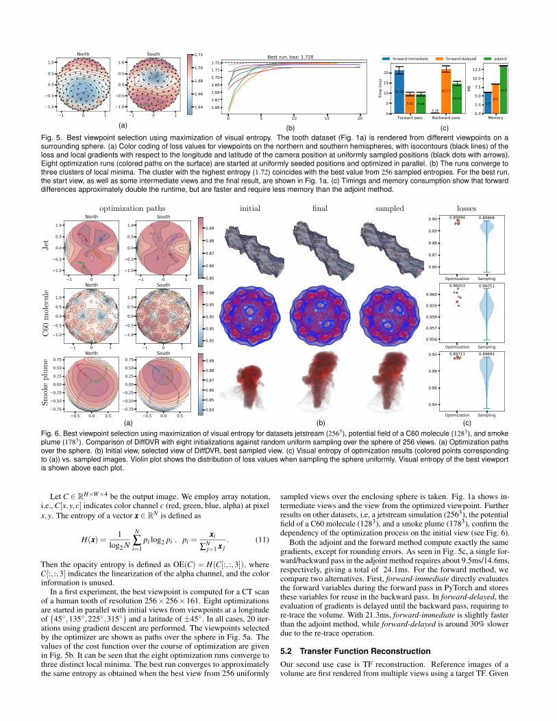
(a) (b) (c)Fig. 5. Best viewpoint selection using maximization of visual entropy. The tooth dataset (Fig. 1a) is rendered from different viewpoints on asurrounding sphere. (a) Color coding of loss values for viewpoints on the northern and southern hemispheres, with isocontours (black lines) of theloss and local gradients with respect to the longitude and latitude of the camera position at uniformly sampled positions (black dots with arrows).Eight optimization runs (colored paths on the surface) are started at uniformly seeded positions and optimized in parallel. (b) The runs converge tothree clusters of local minima. The cluster with the highest entropy (1.72) coincides with the best value from 256 sampled entropies. For the best run,the start view, as well as some intermediate views and the final result, are shown in Fig. 1a. (c) Timings and memory consumption show that forwarddifferences approximately double the runtime, but are faster and require less memory than the adjoint method.

optimization paths initial final sampled losses

Jet

C60molecule

Smokeplume

(a) (b) (c)Fig. 6. Best viewpoint selection using maximization of visual entropy for datasets jetstream (2563), potential field of a C60 molecule (1283), and smokeplume (1783). Comparison of DiffDVR with eight initializations against random uniform sampling over the sphere of 256 views. (a) Optimization pathsover the sphere. (b) Initial view, selected view of DiffDVR, best sampled view. (c) Visual entropy of optimization results (colored points correspondingto (a)) vs. sampled images. Violin plot shows the distribution of loss values when sampling the sphere uniformly. Visual entropy of the best viewportis shown above each plot.

Let C ∈ RH×W×4 be the output image. We employ array notation,

i.e., C[x,y,c] indicates color channel c (red, green, blue, alpha) at pixel

x,y. The entropy of a vector xxx ∈ RN is defined as

H(xxx) =1

log2 N

N

∑i=1

pi log2 pi , pi =xxxi

∑Nj=1 xxx j

. (11)

Then the opacity entropy is defined as OE(C) = H(C[:, :,3]), whereC[:, :,3] indicates the linearization of the alpha channel, and the colorinformation is unused.

In a first experiment, the best viewpoint is computed for a CT scanof a human tooth of resolution 256×256×161. Eight optimizationsare started in parallel with initial views from viewpoints at a longitudeof {45◦,135◦,225◦,315◦} and a latitude of ±45◦. In all cases, 20 iter-ations using gradient descent are performed. The viewpoints selectedby the optimizer are shown as paths over the sphere in Fig. 5a. Thevalues of the cost function over the course of optimization are givenin Fig. 5b. It can be seen that the eight optimization runs converge tothree distinct local minima. The best run converges to approximatelythe same entropy as obtained when the best view from 256 uniformly

sampled views over the enclosing sphere is taken. Fig. 1a shows in-termediate views and the view from the optimized viewpoint. Furtherresults on other datasets, i.e, a jetstream simulation (2563), the potentialfield of a C60 molecule (1283), and a smoke plume (1783), confirm thedependency of the optimization process on the initial view (see Fig. 6).

Both the adjoint and the forward method compute exactly the samegradients, except for rounding errors. As seen in Fig. 5c, a single for-ward/backward pass in the adjoint method requires about 9.5ms/14.6ms,respectively, giving a total of 24.1ms. For the forward method, wecompare two alternatives. First, forward-immediate directly evaluatesthe forward variables during the forward pass in PyTorch and storesthese variables for reuse in the backward pass. In forward-delayed, theevaluation of gradients is delayed until the backward pass, requiring tore-trace the volume. With 21.3ms, forward-immediate is slightly fasterthan the adjoint method, while forward-delayed is around 30% slowerdue to the re-trace operation.

5.2 Transfer Function Reconstruction

Our second use case is TF reconstruction. Reference images of avolume are first rendered from multiple views using a target TF. Given

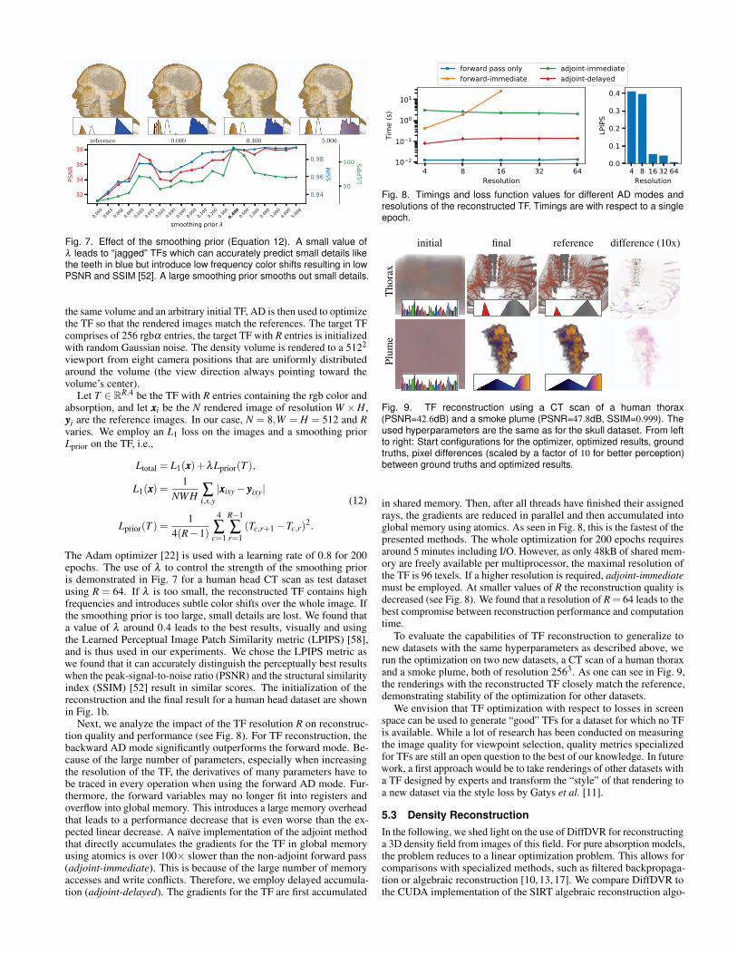
reference 0.000 0.400 5.000

Fig. 7. Effect of the smoothing prior (Equation 12). A small value ofλ leads to “jagged” TFs which can accurately predict small details likethe teeth in blue but introduce low frequency color shifts resulting in lowPSNR and SSIM [52]. A large smoothing prior smooths out small details.

the same volume and an arbitrary initial TF, AD is then used to optimizethe TF so that the rendered images match the references. The target TFcomprises of 256 rgbα entries, the target TF with R entries is initializedwith random Gaussian noise. The density volume is rendered to a 5122

viewport from eight camera positions that are uniformly distributedaround the volume (the view direction always pointing toward thevolume’s center).

Let T ∈ RR,4 be the TF with R entries containing the rgb color and

absorption, and let xxxi be the N rendered image of resolution W ×H,yyyi are the reference images. In our case, N = 8,W = H = 512 and Rvaries. We employ an L1 loss on the images and a smoothing priorLprior on the TF, i.e.,

Ltotal = L1(xxx)+λLprior(T ),

L1(xxx) =1

NWH ∑i,x,y|xxxixy− yyyixy|

Lprior(T ) =1

4(R−1)

4

∑c=1

R−1

∑r=1

(Tc,r+1−Tc,r)2.

(12)

The Adam optimizer [22] is used with a learning rate of 0.8 for 200epochs. The use of λ to control the strength of the smoothing prioris demonstrated in Fig. 7 for a human head CT scan as test datasetusing R = 64. If λ is too small, the reconstructed TF contains highfrequencies and introduces subtle color shifts over the whole image. Ifthe smoothing prior is too large, small details are lost. We found thata value of λ around 0.4 leads to the best results, visually and usingthe Learned Perceptual Image Patch Similarity metric (LPIPS) [58],and is thus used in our experiments. We chose the LPIPS metric aswe found that it can accurately distinguish the perceptually best resultswhen the peak-signal-to-noise ratio (PSNR) and the structural similarityindex (SSIM) [52] result in similar scores. The initialization of thereconstruction and the final result for a human head dataset are shownin Fig. 1b.

Next, we analyze the impact of the TF resolution R on reconstruc-tion quality and performance (see Fig. 8). For TF reconstruction, thebackward AD mode significantly outperforms the forward mode. Be-cause of the large number of parameters, especially when increasingthe resolution of the TF, the derivatives of many parameters have tobe traced in every operation when using the forward AD mode. Fur-thermore, the forward variables may no longer fit into registers andoverflow into global memory. This introduces a large memory overheadthat leads to a performance decrease that is even worse than the ex-pected linear decrease. A naıve implementation of the adjoint methodthat directly accumulates the gradients for the TF in global memoryusing atomics is over 100× slower than the non-adjoint forward pass(adjoint-immediate). This is because of the large number of memoryaccesses and write conflicts. Therefore, we employ delayed accumula-tion (adjoint-delayed). The gradients for the TF are first accumulated

Fig. 8. Timings and loss function values for different AD modes andresolutions of the reconstructed TF. Timings are with respect to a singleepoch.

initial final reference difference (10x)

Thora

xP

lum

e

Fig. 9. TF reconstruction using a CT scan of a human thorax(PSNR=42.6dB) and a smoke plume (PSNR=47.8dB, SSIM=0.999). Theused hyperparameters are the same as for the skull dataset. From leftto right: Start configurations for the optimizer, optimized results, groundtruths, pixel differences (scaled by a factor of 10 for better perception)between ground truths and optimized results.

in shared memory. Then, after all threads have finished their assignedrays, the gradients are reduced in parallel and then accumulated intoglobal memory using atomics. As seen in Fig. 8, this is the fastest of thepresented methods. The whole optimization for 200 epochs requiresaround 5 minutes including I/O. However, as only 48kB of shared mem-ory are freely available per multiprocessor, the maximal resolution ofthe TF is 96 texels. If a higher resolution is required, adjoint-immediatemust be employed. At smaller values of R the reconstruction quality isdecreased (see Fig. 8). We found that a resolution of R = 64 leads to thebest compromise between reconstruction performance and computationtime.

To evaluate the capabilities of TF reconstruction to generalize tonew datasets with the same hyperparameters as described above, werun the optimization on two new datasets, a CT scan of a human thoraxand a smoke plume, both of resolution 2563. As one can see in Fig. 9,the renderings with the reconstructed TF closely match the reference,demonstrating stability of the optimization for other datasets.

We envision that TF optimization with respect to losses in screenspace can be used to generate “good” TFs for a dataset for which no TFis available. While a lot of research has been conducted on measuringthe image quality for viewpoint selection, quality metrics specializedfor TFs are still an open question to the best of our knowledge. In futurework, a first approach would be to take renderings of other datasets witha TF designed by experts and transform the “style” of that rendering toa new dataset via the style loss by Gatys et al. [11].

5.3 Density ReconstructionIn the following, we shed light on the use of DiffDVR for reconstructinga 3D density field from images of this field. For pure absorption models,the problem reduces to a linear optimization problem. This allows forcomparisons with specialized methods, such as filtered backpropaga-tion or algebraic reconstruction [10, 13, 17]. We compare DiffDVR tothe CUDA implementation of the SIRT algebraic reconstruction algo-

Slice RenderingReference ours ASTRA Mitsuba Reference ours ASTRA Mitsuba

Skull

difference (5x): difference (20x):

PSNR: 36.23dB PSNR: 35.00dB PSNR: 33.22dB PSNR: 48.44dB PSNR: 40.35dB PSNR: 44.35dBSSIM: 0.9925 SSIM: 0.8401 SSIM: 0.9885

Plume



Thorax



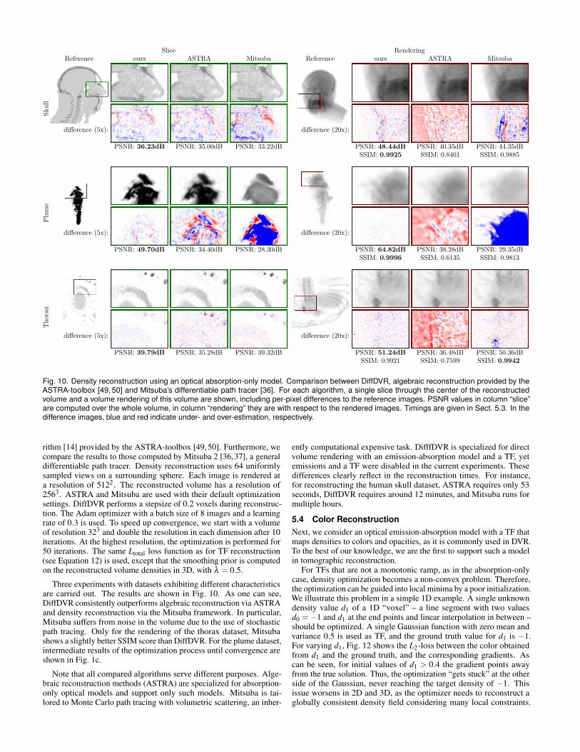
Fig. 10. Density reconstruction using an optical absorption-only model. Comparison between DiffDVR, algebraic reconstruction provided by theASTRA-toolbox [49, 50] and Mitsuba’s differentiable path tracer [36]. For each algorithm, a single slice through the center of the reconstructedvolume and a volume rendering of this volume are shown, including per-pixel differences to the reference images. PSNR values in column “slice”are computed over the whole volume, in column “rendering” they are with respect to the rendered images. Timings are given in Sect. 5.3. In thedifference images, blue and red indicate under- and over-estimation, respectively.

rithm [14] provided by the ASTRA-toolbox [49, 50]. Furthermore, wecompare the results to those computed by Mitsuba 2 [36, 37], a generaldifferentiable path tracer. Density reconstruction uses 64 uniformlysampled views on a surrounding sphere. Each image is rendered ata resolution of 5122. The reconstructed volume has a resolution of2563. ASTRA and Mitsuba are used with their default optimizationsettings. DiffDVR performs a stepsize of 0.2 voxels during reconstruc-tion. The Adam optimizer with a batch size of 8 images and a learningrate of 0.3 is used. To speed up convergence, we start with a volumeof resolution 323 and double the resolution in each dimension after 10iterations. At the highest resolution, the optimization is performed for50 iterations. The same Ltotal loss function as for TF reconstruction(see Equation 12) is used, except that the smoothing prior is computedon the reconstructed volume densities in 3D, with λ = 0.5.

Three experiments with datasets exhibiting different characteristicsare carried out. The results are shown in Fig. 10. As one can see,DiffDVR consistently outperforms algebraic reconstruction via ASTRAand density reconstruction via the Mitsuba framework. In particular,Mitsuba suffers from noise in the volume due to the use of stochasticpath tracing. Only for the rendering of the thorax dataset, Mitsubashows a slightly better SSIM score than DiffDVR. For the plume dataset,intermediate results of the optimization process until convergence areshown in Fig. 1c.

Note that all compared algorithms serve different purposes. Alge-braic reconstruction methods (ASTRA) are specialized for absorption-only optical models and support only such models. Mitsuba is tai-lored to Monte Carlo path tracing with volumetric scattering, an inher-

ently computational expensive task. DifffDVR is specialized for directvolume rendering with an emission-absorption model and a TF, yetemissions and a TF were disabled in the current experiments. Thesedifferences clearly reflect in the reconstruction times. For instance,for reconstructing the human skull dataset, ASTRA requires only 53seconds, DiffDVR requires around 12 minutes, and Mitsuba runs formultiple hours.

5.4 Color ReconstructionNext, we consider an optical emission-absorption model with a TF thatmaps densities to colors and opacities, as it is commonly used in DVR.To the best of our knowledge, we are the first to support such a modelin tomographic reconstruction.

For TFs that are not a monotonic ramp, as in the absorption-onlycase, density optimization becomes a non-convex problem. Therefore,the optimization can be guided into local minima by a poor initialization.We illustrate this problem in a simple 1D example. A single unknowndensity value d1 of a 1D “voxel” – a line segment with two valuesd0 =−1 and d1 at the end points and linear interpolation in between –should be optimized. A single Gaussian function with zero mean andvariance 0.5 is used as TF, and the ground truth value for d1 is −1.For varying d1, Fig. 12 shows the L2-loss between the color obtainedfrom d1 and the ground truth, and the corresponding gradients. Ascan be seen, for initial values of d1 > 0.4 the gradient points awayfrom the true solution. Thus, the optimization “gets stuck” at the otherside of the Gaussian, never reaching the target density of −1. Thisissue worsens in 2D and 3D, as the optimizer needs to reconstruct aglobally consistent density field considering many local constraints.

Tooth Thoraxa) reference b) direct optim. c) color optim. d) density optim. a) reference b) direct optim. c) color optim. d) density optim.

Ren

dering

PSNR: 3.099dB PSNR: 31.158dB PSNR: 31.090dB PSNR: 22.970dB PSNR: 24.092dB PSNR: 24.053dBSSIM: 0.24034 SSIM: 0.97270 SSIM: 0.93954 SSIM: 0.72299 SSIM: 0.83883 SSIM: 0.76007

Slice

Fig. 11. Density optimization for a volume colored via a non-monotonic rgbα-TF using an emission-absorption model. (a) Rendering of the referencevolume of a human tooth and a human thorax. (b) Local minimum of the loss function. (c) Pre-shaded color volume as initialization. (d) Final result ofthe density volume optimization with TF mapping. The second row shows slices through the volumes. Note the colored slice through the pre-shadedcolor volume in (c).

Fig. 12. 1D example for a density optimization with a Gaussian TF withthe optimum at a density of −1.0. For a value > 0.4, the gradient facesaway from the optimum.

This failure case is also shown in Fig. 11b, where the tooth datasetcannot be reconstructed faithfully due to the initialization with a poorlymatching initial field.

To overcome this shortcoming, it is crucial to start the optimizationwith an initial guess that is not “too far” from the ground truth in thehigh-dimensional parameter space. We account for this by proposingthe following optimization pipeline: First, a pre-shaded color volumeof resolution 2563 (Fig. 11c) is reconstructed from images using thesame multi-resolution optimization as in the case of an absorption-onlymodel. The color volume stores the rgb-emission and scalar absorptionper voxel, instead of a scalar density value that is mapped to color via aTF. By using this color volume, trapping into local minima with non-monotonic TFs can be avoid. Intermediate results of the optimizationprocess until convergence are shown in Fig. 1d for the tooth dataset.Then, density values that match the reconstructed colors after applyingthe TF are estimated. For each voxel, 256 random values are sampled,converted to color via the TF, and the best match is chosen. To avoidinconsistencies between neighboring voxels, an additional loss termpenalises differences to neighbors. Let (τT ,CT ) be the target colorfrom the color volume and d the sampled density with mapped colorτ(d),C(d), then the cost function is

C (d) = ||CT −C(d)||22 +α log(1+ |τT − τ(d)|)+β ∑i∈N

(d−di)2.

(13)Here, α and β are weights, and N loops over the 6-neighborhood ofthe current voxel. The logarithm accounts for the vastly different scalesof the absorption, similar to an inverse of the transparency integralEquation 1. In the example, we set α = 1/max(τT ) to normalize forthe maximal absorption in the color volume, and β = 1. This processis repeated until the changes between subsequent iterations fall belowa certain threshold, or a prescribed number of iterations have beenperformed.

Finally, the estimated density volume is used as initialization for theoptimization of the density volume from the rendered images (Fig. 11d).We employ the same loss Ltotal as before with a smoothing prior ofλ = 20. The total runtime for a 2563 volume is roughly 50 minutes.Even though the proposed initialization overcomes to a certain extentthe problem of non-convexity and yields reasonable results, Fig. 11indicates that some fine details are lost and spurious noise remains.We attribute this to remaining ambiguities in the sampling of densitiesfrom colors that still lead to suboptimal minima in the reconstruction.This also shows in the slice view of Fig. 11d, especially for the thoraxdataset. Here, some areas that are fully transparent due to the TF arearbitrarily mapped to a density value of zero, while the reference has adensity around 0.5 – between the peaks of the TF – in these areas.

6 CONCLUSION

In this work, we have introduced a framework for differentiable directvolume rendering (DiffDVR), and we have demonstrated its use ina number of different tasks related to data visualization. We haveshown that differentiability of the direct volume rendering process withrespect to the viewpoint position, the TF, and the volume densities isfeasible, and can be performed at reasonable memory requirements andsurprisingly good performance.

Our results indicate the potential of the proposed framework toautomatically determine optimal parameter combinations regardingdifferent loss functions. This makes DiffDVR in particular interestingin combination with neural networks. Such networks might be used asloss functions – providing blackboxes, which steer DiffDVR to an opti-mal output for training purposes, e.g., to synthesize volume-renderedimagery for transfer learning tasks. Furthermore, derivatives with re-spect to the volume from rendered images promise the application toscene representation networks trained in screen space instead of frompoints in object space. We see this as one of the most interesting futureworks, spawning future research towards the development of techniquesthat can convert large data to a compact representation -– a code -– thatcan be permanently stored and accessed by a network-based visualiza-tion. Besides neural networks, we imagine possible applications in thedevelopment of lossy compression algorithms, e.g. via wavelets, wherethe compression rate is not determined by losses in world space, butby the quality of rendered images. The question we will address inthe future is how to generate such (visualization-)task-dependent codesthat can be intertwined with differentiable renderers.

ACKNOWLEDGMENTS

The authors wish to thank Jakob Wenzel and Merlin Nimier-David fortheir help and valuable suggestions on the Mitsuba 2 framework.

REFERENCES

[1] M. Abadi, P. Barham, J. Chen, Z. Chen, A. Davis, J. Dean, M. Devin,

S. Ghemawat, G. Irving, M. Isard, et al. Tensorflow: A system for large-

scale machine learning. In 12th {USENIX} symposium on operatingsystems design and implementation ({OSDI} 16), pp. 265–283, 2016.

[2] M. Bartholomew-Biggs, S. Brown, B. Christianson, and L. Dixon. Auto-

matic differentiation of algorithms. Journal of Computational and AppliedMathematics, 124(1):171–190, 2000. Numerical Analysis 2000. Vol. IV:

Optimization and Nonlinear Equations. doi: 10.1016/S0377-0427(00)

00422-2

[3] M. Berger, J. Li, and J. A. Levine. A generative model for volume

rendering. IEEE transactions on visualization and computer graphics,

25(4):1636–1650, 2018.

[4] M. R. Bolin and G. W. Meyer. A perceptually based adaptive sampling

algorithm. In Proceedings of the 25th Annual Conference on ComputerGraphics and Interactive Techniques, SIGGRAPH ’98, p. 299–309. As-

sociation for Computing Machinery, New York, NY, USA, 1998. doi: 10.

1145/280814.280924

[5] U. D. Bordoloi and H.-W. Shen. View selection for volume rendering. In

VIS 05. IEEE Visualization, 2005., pp. 487–494. IEEE, 2005.

[6] L. Q. Campagnolo, W. Celes, and L. H. de Figueiredo. Accurate volume

rendering based on adaptive numerical integration. In 2015 28th SIB-GRAPI Conference on Graphics, Patterns and Images, pp. 17–24. IEEE,

2015.

[7] M. Chen and H. Jaenicke. An information-theoretic framework for visu-

alization. IEEE Transactions on Visualization and Computer Graphics,

16(6):1206–1215, 2010.

[8] C. D. Correa and K.-L. Ma. Visibility histograms and visibility-driven

transfer functions. IEEE Transactions on Visualization and ComputerGraphics, 17(2):192–204, 2010.

[9] J. Danskin and P. Hanrahan. Fast algorithms for volume ray tracing. In

Proceedings of the 1992 Workshop on Volume Visualization, VVS ’92, p.

91–98. Association for Computing Machinery, New York, NY, USA, 1992.

doi: 10.1145/147130.147155

[10] D. Dudgeon, R. Mersereau, and R. Merser. Multidimensional digital signal

processing. prentice hall. Englewood Cliffs, NJ, 19842, 1984.

[11] L. A. Gatys, A. S. Ecker, and M. Bethge. Image style transfer using

convolutional neural networks. In Proceedings of the IEEE conference oncomputer vision and pattern recognition, pp. 2414–2423, 2016.

[12] I. Gkioulekas, S. Zhao, K. Bala, T. Zickler, and A. Levin. Inverse volume

rendering with material dictionaries. ACM Transactions on Graphics(TOG), 32(6):1–13, 2013.

[13] R. Gordon, R. Bender, and G. T. Herman. Algebraic reconstruction

techniques (art) for three-dimensional electron microscopy and x-ray pho-

tography. Journal of Theoretical Biology, 29(3):471–481, 1970. doi: 10.

1016/0022-5193(70)90109-8

[14] J. Gregor and T. Benson. Computational analysis and improvement of sirt.

IEEE Transactions on Medical Imaging, 27(7):918–924, 2008. doi: 10.

1109/TMI.2008.923696

[15] M. Haidacher, D. Patel, S. Bruckner, A. Kanitsar, and M. E. Groller.

Volume visualization based on statistical transfer-function spaces. In

2010 IEEE Pacific Visualization Symposium (PacificVis), pp. 17–24. IEEE,

2010.

[16] W. He, J. Wang, H. Guo, K.-C. Wang, H.-W. Shen, M. Raj, Y. S. Nashed,

and T. Peterka. Insitunet: Deep image synthesis for parameter space

exploration of ensemble simulations. IEEE transactions on visualizationand computer graphics, 26(1):23–33, 2019.

[17] G. T. Herman. Fundamentals of computerized tomography: image recon-struction from projections. Springer Science & Business Media, 2009.

[18] W. Jakob. Enoki: structured vectorization and differentiation

on modern processor architectures, 2019. https://github.com/

mitsuba-renderer/enoki.

[19] G. Ji and H.-W. Shen. Dynamic view selection for time-varying volumes.

IEEE Transactions on Visualization and Computer Graphics, 12(5):1109–

1116, 2006.

[20] H. Kato, D. Beker, M. Morariu, T. Ando, T. Matsuoka, W. Kehl,

and A. Gaidon. Differentiable rendering: A survey. arXiv preprintarXiv:2006.12057, 2020.

[21] H. Kato, Y. Ushiku, and T. Harada. Neural 3d mesh renderer. In Proceed-ings of the IEEE conference on computer vision and pattern recognition,

pp. 3907–3916, 2018.

[22] D. P. Kingma and J. Ba. Adam: A method for stochastic optimization.

arXiv preprint arXiv:1412.6980, 2014.

[23] A. Kratz, J. Reininghaus, M. Hadwiger, and I. Hotz. Adaptive screen-space

sampling for volume ray-casting. ZIB-Report, 2011.

[24] T.-M. Li, M. Aittala, F. Durand, and J. Lehtinen. Differentiable monte

carlo ray tracing through edge sampling. ACM Transactions on Graphics(TOG), 37(6):1–11, 2018.

[25] S. Liu, S. Saito, W. Chen, and H. Li. Learning to infer implicit surfaces

without 3d supervision. NeurIPS, 2019.

[26] M. M. Loper and M. J. Black. Opendr: An approximate differentiable

renderer. In European Conference on Computer Vision, pp. 154–169.

Springer, 2014.

[27] R. Maciejewski, Y. Jang, I. Woo, H. Janicke, K. P. Gaither, and D. S.

Ebert. Abstracting attribute space for transfer function exploration and

design. IEEE Transactions on Visualization and Computer Graphics,

19(1):94–107, 2012.

[28] R. Marques, C. Bouville, M. Ribardiere, L. P. Santos, and K. Bouatouch.

Spherical fibonacci point sets for illumination integrals. Computer Graph-ics Forum, 32(8):134–143, 2013. doi: 10.1111/cgf.12190

[29] J. Martschinke, S. Hartnagel, B. Keinert, K. Engel, and M. Stamminger.

Adaptive temporal sampling for volumetric path tracing of medical data.

Computer Graphics Forum, 38(4):67–76, 2019. doi: 10.1111/cgf.13771

[30] N. Max. Optical models for direct volume rendering. IEEE Transactionson Visualization and Computer Graphics, 1(2):99–108, 1995.

[31] A. McNamara, A. Treuille, Z. Popovic, and J. Stam. Fluid control using

the adjoint method. ACM Trans. Graph., 23(3):449–456, Aug. 2004. doi:

10.1145/1015706.1015744

[32] N. Morrical, W. Usher, I. Wald, and V. Pascucci. Efficient space skipping

and adaptive sampling of unstructured volumes using hardware accelerated

ray tracing. In 2019 IEEE Visualization Conference (VIS), pp. 256–260,

2019. doi: 10.1109/VISUAL.2019.8933539

[33] R. D. Neidinger. Introduction to automatic differentiation and matlab

object-oriented programming. SIAM review, 52(3):545–563, 2010.

[34] T. Nguyen-Phuoc, C. Li, S. Balaban, and Y.-L. Yang. Rendernet: A deep

convolutional network for differentiable rendering from 3d shapes. arXivpreprint arXiv:1806.06575, 2018.

[35] M. Niemeyer, L. Mescheder, M. Oechsle, and A. Geiger. Differentiable

volumetric rendering: Learning implicit 3d representations without 3d

supervision. In Proceedings of the IEEE/CVF Conference on ComputerVision and Pattern Recognition (CVPR), June 2020.

[36] M. Nimier-David, S. Speierer, B. Ruiz, and W. Jakob. Radiative back-

propagation: An adjoint method for lightning-fast differentiable rendering.

Transactions on Graphics (Proceedings of SIGGRAPH), 39(4), July 2020.

doi: 10.1145/3386569.3392406

[37] M. Nimier-David, D. Vicini, T. Zeltner, and W. Jakob. Mitsuba 2: A

retargetable forward and inverse renderer. ACM Trans. Graph., 38(6), Nov.

2019. doi: 10.1145/3355089.3356498

[38] NVidia. Cuda nvrtc, 2021. https://docs.nvidia.com/cuda/nvrtc/

index.html.

[39] J. Painter and K. Sloan. Antialiased ray tracing by adaptive progressive

refinement. In Proceedings of the 16th annual conference on Computergraphics and interactive techniques, pp. 281–288, 1989.

[40] A. Paszke, S. Gross, F. Massa, A. Lerer, J. Bradbury, G. Chanan, T. Killeen,

Z. Lin, N. Gimelshein, L. Antiga, A. Desmaison, A. Kopf, E. Yang, Z. De-

Vito, M. Raison, A. Tejani, S. Chilamkurthy, B. Steiner, L. Fang, J. Bai,

and S. Chintala. Pytorch: An imperative style, high-performance deep

learning library. In H. Wallach, H. Larochelle, A. Beygelzimer, F. d'Alche-

Buc, E. Fox, and R. Garnett, eds., Advances in Neural Information Pro-cessing Systems 32, pp. 8024–8035. Curran Associates, Inc., 2019.

[41] F. Petersen, A. H. Bermano, O. Deussen, and D. Cohen-Or. Pix2vex:

Image-to-geometry reconstruction using a smooth differentiable renderer.

arXiv preprint arXiv:1903.11149, 2019.

[42] H. Rhodin, N. Robertini, C. Richardt, H.-P. Seidel, and C. Theobalt. A

versatile scene model with differentiable visibility applied to generative

pose estimation. In Proceedings of the IEEE International Conference onComputer Vision, pp. 765–773, 2015.

[43] M. Ruiz, A. Bardera, I. Boada, and I. Viola. Automatic transfer functions

based on informational divergence. IEEE Transactions on Visualizationand Computer Graphics, 17(12):1932–1941, 2011.

[44] V. Sitzmann, M. Zollhofer, and G. Wetzstein. Scene representation

networks: Continuous 3d-structure-aware neural scene representations.

NeurIPS, 2019.

[45] S. Takahashi, I. Fujishiro, Y. Takeshima, and T. Nishita. A feature-driven

approach to locating optimal viewpoints for volume visualization. In VIS

05. IEEE Visualization, 2005., pp. 495–502. IEEE, 2005.

[46] Y. Tao, H. Lin, H. Bao, F. Dong, and G. Clapworthy. Structure-aware

viewpoint selection for volume visualization. In 2009 IEEE Pacific Visual-ization Symposium, pp. 193–200. IEEE, 2009.

[47] Y. Tao, Q. Wang, W. Chen, Y. Wu, and H. Lin. Similarity voting based

viewpoint selection for volumes. In Computer graphics forum, vol. 35, pp.

391–400. Wiley Online Library, 2016.

[48] A. Tewari, O. Fried, J. Thies, V. Sitzmann, S. Lombardi, K. Sunkavalli,

R. Martin-Brualla, T. Simon, J. Saragih, M. Nießner, et al. State of the art

on neural rendering. In Computer Graphics Forum, vol. 39, pp. 701–727.

Wiley Online Library, 2020.

[49] W. van Aarle, W. J. Palenstijn, J. Cant, E. Janssens, F. Bleichrodt,

A. Dabravolski, J. D. Beenhouwer, K. J. Batenburg, and J. Sijbers. Fast

and flexible x-ray tomography using the astra toolbox. Opt. Express,

24(22):25129–25147, Oct 2016. doi: 10.1364/OE.24.025129

[50] W. van Aarle, W. J. Palenstijn, J. De Beenhouwer, T. Altantzis, S. Bals,

K. J. Batenburg, and J. Sijbers. The astra toolbox: A platform for advanced

algorithm development in electron tomography. Ultramicroscopy, 157:35–

47, 2015. doi: 10.1016/j.ultramic.2015.05.002

[51] P.-P. Vazquez, E. Monclus, and I. Navazo. Representative views and paths

for volume models. In International Symposium on Smart Graphics, pp.

106–117. Springer, 2008.

[52] Z. Wang, A. C. Bovik, H. R. Sheikh, and E. P. Simoncelli. Image quality

assessment: from error visibility to structural similarity. IEEE transactionson image processing, 13(4):600–612, 2004.

[53] S. Weiss, M. Chu, N. Thuerey, and R. Westermann. Volumetric isosurface

rendering with deep learning-based super-resolution. IEEE Transactionson Visualization and Computer Graphics, pp. 1–1, 2019. doi: 10.1109/

TVCG.2019.2956697

[54] S. Weiss, M. Isık, J. Thies, and R. Westermann. Learning adaptive sam-

pling and reconstruction for volume visualization. IEEE Transactions onVisualization and Computer Graphics, pp. 1–1, 2020. doi: 10.1109/TVCG

.2020.3039340

[55] R. E. Wengert. A simple automatic derivative evaluation program. Com-munications of the ACM, 7(8):463–464, 1964.

[56] Q. Xu, S. Bao, R. Zhang, R. Hu, and M. Sbert. Adaptive sampling for

monte carlo global illumination using tsallis entropy. In InternationalConference on Computational and Information Science, pp. 989–994.

Springer, 2005.

[57] C. Yang, Y. Li, C. Liu, and X. Yuan. Deep learning-based viewpoint rec-

ommendation in volume visualization. Journal of Visualization, 22(5):991–

1003, 2019.

[58] R. Zhang, P. Isola, A. A. Efros, E. Shechtman, and O. Wang. The unrea-

sonable effectiveness of deep features as a perceptual metric. In CVPR,

2018.

[59] L. Zhou and C. Hansen. Transfer function design based on user selected

samples for intuitive multivariate volume exploration. In 2013 IEEEPacific Visualization Symposium (PacificVis), pp. 73–80. IEEE, 2013.

Differentiable Direct Volume Rendering

Documents

Transcript of Differentiable Direct Volume Rendering