Difference-in-Differences with GeocodedMicrodata*Kyle Butts†October 22, 2021

This paper formalizes a common approach for estimating effects of treatment at a specificlocation using geocoded microdata. This estimator compares units immediately next totreatment (an inner-ring) to units just slightly further away (an outer-ring). I introduce intu-itive assumptions needed to identify the average treatment effect among the affected unitsand illustrates pitfalls that occur when these assumptions fail. Since one of these assump-tions requires knowledge of exactly how far treatment effects are experienced, I proposea new method that relaxes this assumption and allows for nonparametric estimation usingpartitioning-based least squares developed in Cattaneo et al. (2019a,b). Since treatment ef-fects typically decay/change over distance, this estimator improves analysis by estimating atreatment effect curve as a function of distance from treatment. This is contrast to the tra-ditional method which, at best, identifies the average effect of treatment. To illustrate theadvantages of this method, I show that Linden and Rockoff (2008) under estimate the ef-fects of increased crime risk on home values closest to the treatment and overestimate howfar the effects extend by selecting a treatment ring that is too wide.

JEL-Classification: C13, C14, C18Keywords: Spatial Econometrics, Difference-in-Differences, Nonparametric Estimation

*I am grateful to Taylor Jaworski, Damian Clarke, Alexander Bentz, James Flynn, Brach Champion, and Han-nah Denker for the helpful insights.

†University of Colorado, Boulder. Email: kyle.butts@colorado.edu.1

arX

iv:2

110.

1019

2v1

[ec

on.E

M]

19

Oct

202

1

1— Introduction

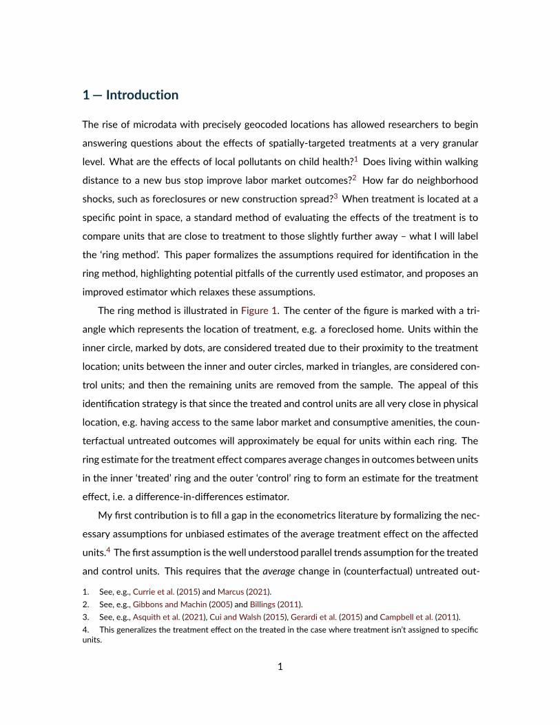
The rise of microdata with precisely geocoded locations has allowed researchers to beginanswering questions about the effects of spatially-targeted treatments at a very granularlevel. What are the effects of local pollutants on child health?1 Does living within walkingdistance to a new bus stop improve labor market outcomes?2 How far do neighborhoodshocks, such as foreclosures or new construction spread?3 When treatment is located at aspecific point in space, a standard method of evaluating the effects of the treatment is tocompare units that are close to treatment to those slightly further away – what I will labelthe ‘ring method’. This paper formalizes the assumptions required for identification in thering method, highlighting potential pitfalls of the currently used estimator, and proposes animproved estimator which relaxes these assumptions.

The ring method is illustrated in Figure 1. The center of the figure is marked with a tri-angle which represents the location of treatment, e.g. a foreclosed home. Units within theinner circle, marked by dots, are considered treated due to their proximity to the treatmentlocation; units between the inner and outer circles, marked in triangles, are considered con-trol units; and then the remaining units are removed from the sample. The appeal of thisidentification strategy is that since the treated and control units are all very close in physicallocation, e.g. having access to the same labor market and consumptive amenities, the coun-terfactual untreated outcomes will approximately be equal for units within each ring. Thering estimate for the treatment effect compares average changes in outcomes between unitsin the inner ‘treated’ ring and the outer ‘control’ ring to form an estimate for the treatmenteffect, i.e. a difference-in-differences estimator.

My first contribution is to fill a gap in the econometrics literature by formalizing the nec-essary assumptions for unbiased estimates of the average treatment effect on the affectedunits.4 The first assumption is thewell understood parallel trends assumption for the treatedand control units. This requires that the average change in (counterfactual) untreated out-1. See, e.g., Currie et al. (2015) and Marcus (2021).2. See, e.g., Gibbons and Machin (2005) and Billings (2011).3. See, e.g., Asquith et al. (2021), Cui and Walsh (2015), Gerardi et al. (2015) and Campbell et al. (2011).4. This generalizes the treatment effect on the treated in the case where treatment isn’t assigned to specificunits.

1

Figure 1—Rings Method

comes in the treated ring is equal to the average change in the control ring. This allows thecontrol units to estimate the counterfactual trend for the treated units.

The second assumption requires the researcher to correctly identify how far treatmenteffects are experienced (the inner ring). This is a very strict assumption that when not satis-fied, causes biased estimates of the treatment effect. If the treated ring is too narrow, thenunits in the control ring experience effects of treatment and the change among ‘control’ unitswould no longer identify the counterfactual trend. On the other hand, if the treated ring istoo wide, then the zero treatment effect of some unaffected units are averaged into thechange among ‘treated’ units. Therefore, results will be attenuated towards zero.

Since researchers often do not know how far treatment effects extend in most circum-stances, I propose an estimator that replaces the second assumption with a less strict as-sumption by using a nonparametric, partitioning-based, least square estimator (Cattaneoet al. 2019a,b). My proposed methodology estimates the treatment effect curve as a func-tion of distance by using many rings rather than trying to estimate the average treatmenteffect with one inner ring. This method requires that treatment effects become zero some-where between the distance of 0 and the control ring without the need to specify the exactdistance. It however requires a stronger assumption that the counterfactual trend is con-stant across distance.5 This new assumption is more strict in that the standard method only5. Note that the original requirement is that the average change in each ring is equal but allows variation acrossdistance.

2

requires that parallel trends holds on average in each ring. However, researchers motivatethe identification strategy by saying within a small distance from treatment that units aresubject to a common set of shocks which implies the more strict assumption. While this as-sumption is not directly testable, the estimator creates a set of point estimates of treatmenteffects that can be used to visually inspect the plausability of the assumption. If after somedistance, treatment effects become centered at zero, this suggests that common trends hold,akin to the pre-trends test in event study regressions.

The nonparametric approach allows the researcher to get a more complete picture ofhow the intervention affects units at various distances rather than estimating an “overalleffect”. For example, the construction of a new bus-stop potentially creates net costs to im-mediate neighbors while providing net benefits for homes slightly further away. Estimationof the treatment effect curve can illustrate these different effects that the “overall effect”would mask. In this case, the average effect could be zero even though most units experi-ence non-zero effects.1.1. Relation to Literature

This paper relates to a few papers that address difficulties with using the rings method forcausal effect estimation. In the online appendix, Gerardi et al. (2015) discuss the problemthat if the treated ring is defined too narrowly, then control units will be affected by treat-ment causing a biased estimate of the counterfactual trend. Sullivan (2017) discusses theproblem more formally and derives that the bias will be the difference in treatment effectsexperienced by the ‘treated’ ring and the ‘control’ ring. My paper expands on the resultsof Sullivan (2017) by including the additional source of bias that can result from a violationof parallel trends. Other researchers have recognized that estimating a single average treat-ment effect is less informative than a treatment effect curve. They solve this by using mul-tiple rings to estimate treatment effects at different distances (e.g. Alexander et al. (2019),Casey et al. (2018), Di Tella and Schargrodsky (2004)). However, this approach selects mul-tiple rings in an ad-hoc manner, still requires treatment effects to become zero after theouter-most treatment ring, and is prone to problems of specification searching. The currentstudy’s proposed estimator selects the number and location of rings in a data-driven way

3

and does not require correct specification of where treatment effects become zero.Diamond and McQuade (2019) propose a nonparametric estimator aimed at estimating

a treatment effect surface. They use two-dimensions (latitude/longitude) to better approx-imate a smooth change in counterfactual outcomes (e.g. north-west and south-east fromtreatment might have different treatment effects). My method, instead, uses a singular mea-sure of distancewhich pools units at similar distances but different directions from treatmentand therefore delivers more precise estimates. However, the treatment effect estimate maymask heterogeneity of effects at different directions. If a researcher has a reason to suspectsignificant heterogeneity, then their proposed estimator will make a better fit.

This paper also contributes to a small literature on difference-in-differences estimatorsfrom a spatial lens (Butts 2021, Clarke 2017, Berg and Streitz 2019, Verbitsky-Savitz andRaudenbush 2012, Delgado and Florax 2015). These papers address instances where treat-ment is well defined by administrative boundaries but spillovers cause problems of definingwho is ‘treated’ and at what level of exposure. Butts (2021) and Clarke (2017) both recom-mend a method of using many rings to estimate treatment effects similar to the proposednonparametric estimator. Clarke (2017) does specify a cross-validation approach for select-ing rings, but does not specify that this result requires common local trends. Since this paperfocuses on local shocks where constant parallel trends are plausible, I am able to provide adata-driven approach to choosing rings.

Last, there is a growing literature around design-based estimation of treatment effects inthe presence of spillover effects (?Aronow et al. 2020). Aronow et al. (2021) specifically dis-cuss estimation of what this paper calls the treatment effect curve, or the average treatmenteffect at a certain distance away from treatment. This paper compliments this literature byintroducing model-based assumptions for cases where treatment is not assigned followingan experimental design.

2— Example of Problem

To illustrate the methodological difficulties in this method, I present an illustriative example.Suppose that an overgrown empty lot in a high-poverty neighborhood is cleaned up by the

4

Figure 2—Example of Problems with Ad-Hoc Ring Selection

Notes: This figure shows an example of the ring method. For each panel, the inner ring marks units considered‘treated’, the outer ring marks units considered ‘control’ units, and the rest of the observations are removed fromthe sample. Then average changes in outcomes are compared between the treated and the control units to forma treatment effect estimate.

city and the outcome of interest is home prices. The researcher observes a panel of homesales before and after the lot is cleaned. Cleaning up the lot causes home values to goup directly nearby and as you move away from the lot, the positive treatment effect willdecay to zero effect at, say, 3/4 of a mile. Since treatment is targeted to the high povertyneighborhood, comparisons with other neighborhoods in the cities could be biased if theneighborhood home prices are on different trends. Hence, the researcher wants to lookonly at the homes in the immediate neighborhood.

Figure 2 shows a plot of simulated data from this example. The black line is treatmenteffect at different distances from the empty lot and the grey line is the underlying (constant)counterfactual change in home prices, normalized to 0. Panel (a) of Figure 2 shows thebest-case scenario where the treated ring is correctly specified. The two horizontal lines

5

show the average change in outcome in the treated ring and the control ring. The treatmenteffect estimate, τ , is the difference between these two averages. However, this singularnumber masks over a large amount of treatment effect heterogeneity with units very closeto treatment having a treatment effect double that of τ and units near 3/4 miles experiencea treatment efffect half as large as τ . For this reason, even if a researcher identifies thecorrect average treatment effect, they are masking a lot of heterogeneity that is potentiallyinteresting. Therefore, later in this paper I recommend nonparametrically estimating thetreatment effect curve as a function of distance rather than using average effect.

However, the researcher does not typically know the distance at which treatment effectsstop. Panels (b) and (c) highlights how treatment effect estimates change with a change inring distances. Panel (b) showswhen the ‘treatment’ ring is toowide. In this case, some of theunits in the treatment ring receive no effect from treatment and thereforemakes the averagetreament effect among units in the treatment ring smaller. Therefore when the treated ringis too large, the estimated treatment effect is too small. Panel (c) of Figure 2 shows theopposite case, where the treated ring is too narrow. In this case, there are some units inthe ‘control’ ring that experience treatment effects. Hence, the average change in outcomeamong the control unit is too large. This does not, though, decrease the treatment effectas one may suspect. Since the treatment effect decays with distance, the average changein outcome among the more narrow ‘treatment’ ring is larger than the correct specification.The estimated treatment effect in this case grows, but it is not clear more generally whetherthe treatment effect will increase or decrease.6 From these three examples, it’s clear thatthe estimation strategy requires researchers to know the exact distance at which treatmenteffects become zero. Since this is a very demanding assumption, I propose an improvedestimator in section 4 that relaxes this assumption.

Often times, researchers try multiple sets of rings and if the estimated effect remainssimilar across specifications, they assume the results are ‘robust’. Panel (d) of Figure 2 showsan example of why this a problem. If Panel (c) was the researchers’ original specification andPanel (d) was run as a robustness check, then the researcher would be quite confident intheir results even though the estimate is too large in both cases. Now, I turn to econometric6. This primarily depends on the curvature of the treatment effect curve.

6

theory in order to formalize the intuition developed in this section.

3— Theory

Now, I develop econometric theory to formalize the intuition developed in the previoussection. A researcher observes panel data of a random sample of units i at times t = 0, 1

located in space at point θi = (xi, yi). Treatment occurs at a location θ = (x, y) betweenperiods. Therefore, units differ in their distance to treatment, defined by Disti ≡ d(θi, θ) forsome distance metric d (e.g. Euclidean distance) with a distribution function F . Outcomesare given by

Yit = µi + τi1t=1 + λi1t=1 + uit, (1)where µi is unit-specific time-invariant factors, λi is the change in outcomes due to non-treatment shocks in period 1, τi is unit i’s treatment effect. Both λ and τ can be split into asystematic function of distance z(Disti) and an idiosyncratic term zi ≡ zi − z(Disti) with zbeing τ and λ. τ(d) is the average effect of treatment at a given distance and λ(d) summarizeshow covariates and shocks change over distance. Therefore, we could rewrite our model as

Yit = µi + τ(Disti)1t=1 + λ(Disti)1t=1 + εit, (2)

where ε = uit + τi + λi which is uncorrelated with distance to treatment. Researchers aretrying to identify the average treatment effect on units experiencing treatment effects, i.e.τ = E [τi | τ(Disti) > 0].Assumption 1 (Random Sampling). The observed data consists of {Yi1, Yi0,Disti} which isindependent and identically distributed.

Taking first-differences of our model, we have ∆Yit = τ(Disti) + λ(Disti) + ∆εit. It isclear that τ(Disti) and λ(Disti) are not seperately identified unless additional assumptionsare imposed. The central identifying assumption that researchers claim when using the ringmethod is that counterfactual trends likely evolve smoothly over distance, so that λ(Disti)is approximately constant within a small distance from treatment. This is formalized in thecontext of our outcome model by the following assumption.

7

Assumption 2 (Local Parallel Trends). For a distance d, we say that ‘local parallel trends’ holdif for all positive d, d′ ≤ d, then λ(d) = λ(d′).

This assumption requires that, in the absence of treatment, outcomes would evolve thesame at every distance from treatment within a certain maximum distance, d. To clarify theassumption, it is helpful to think of ways that it can fail. First, if treatment location is targetedbased on trends within a small-area/neighborhood, then trends would not be constant withinthe control ring. Second, if units sort either towards or away from treatment in a way thatis systematically correlated with the outcome variable, then the compositional change cancause a violation in trends over time. Note that Local Parallel Trends implies the standardassumption that parallel trends holds on average between the treated and control rings:Assumption 3 (Average Parallel Trends). For a pair of distances dt and dc, we say that ‘aver-age parallel trends’ hold if E [λd | 0 ≤ d ≤ dt] = E [λd | dt < d ≤ dc].

If Local Parallel Trends holds for some dc, then our first-difference equation can be sim-plified to ∆Yit = τ(Disti) + λ + ∆εit where λ is some constant for units in the subsampleD ≡ {i : Disti ≤ dc}. Therefore, the treatment effect curve τ(Disti) is identifiable up to aconstant under Assumption 2. To identify τ(Disti) seperately from the constant, researcherswill often claim that treatment effects stop occuring before some distance dt < dc. This isformalized in the following assumption.Assumption 4 (Correct dt). A distance dt satisfies this assumption if (i) for all d ≤ dt, τ(d) > 0

and for all d > dt, τ(d) = 0 and (ii) F (dc)− F (dt) > 0.With this assumption, the first difference equation simplifies to ∆Yit = λ+∆εit for units

with dt < Disti < dc. These units therefore identify λ. The ‘ring method’ is the followingprocedure. Researchers select a pair of distances dt < dc which define the “treated” and“control” groups. These groups are defined by Dt ≡ {i : 0 ≤ Disti ≤ dt} and Dc ≡ {i : dt <

Disti ≤ dc}. On the subsample of observations defined by D ≡ Dt ∪ Dc, they estimate thefollowing regression:

∆Yit = β0 + β11i∈Dt + uit. (3)

8

From standard results for regressions involving only indicators, β1 is the difference-in-differences estimator with the following expectation:

E[β1

]= E [∆Yit | Dt]− E [∆Yit | Dc] .

This estimate is decomposed in the following proposition.7Proposition 1 (Decomposition of Ring Estimate). Given that units follow model (2),(i) The estimate of β1 in (3) has the following expectation:

E[β1

]= E [∆Yit | Dt]− E [∆Yit | Dc]

= E [τ(Dist) | Dt]− E [τ(Dist) | Dc]︸ ︷︷ ︸Difference in Treatment Effect+E [λ(Dist) | Dt]− E [λ(Dist) | Dc]︸ ︷︷ ︸Difference in Trends

.

(ii) If dc satisfies Local Parallel Trends or, more weakly, if dt and dc satisfy Average ParallelTrends, then

E[β1

]= E [τ(Dist) | Dt]− E [τ(Dist) | Dc]︸ ︷︷ ︸Difference in Treatment Effect

.

(iii) If dc satisfies Local Parallel Trends and dt satisfies Assumption 4, then

E[β1

]= τ .

Part (i) of this proposition shows that the estimate is the sum of two differences. Thefirst difference is the difference in average treatment effect among units in the treated ringand units in the control ring. The second difference is the difference in counterfactual trendsbetween the treated and control rings. This presents two possible problems. If some unitsin the control group experience effects from treatment, the average of these effects will besubtracted from the estimate. Second, since treatment can be targeted, the treated ringcould be on a different trend than units further away and hence control units do not serveas a good counterfactual for treated units.7. A similar derivation of part (i) is found in Sullivan (2017) but does not include difference in parallel trends.

9

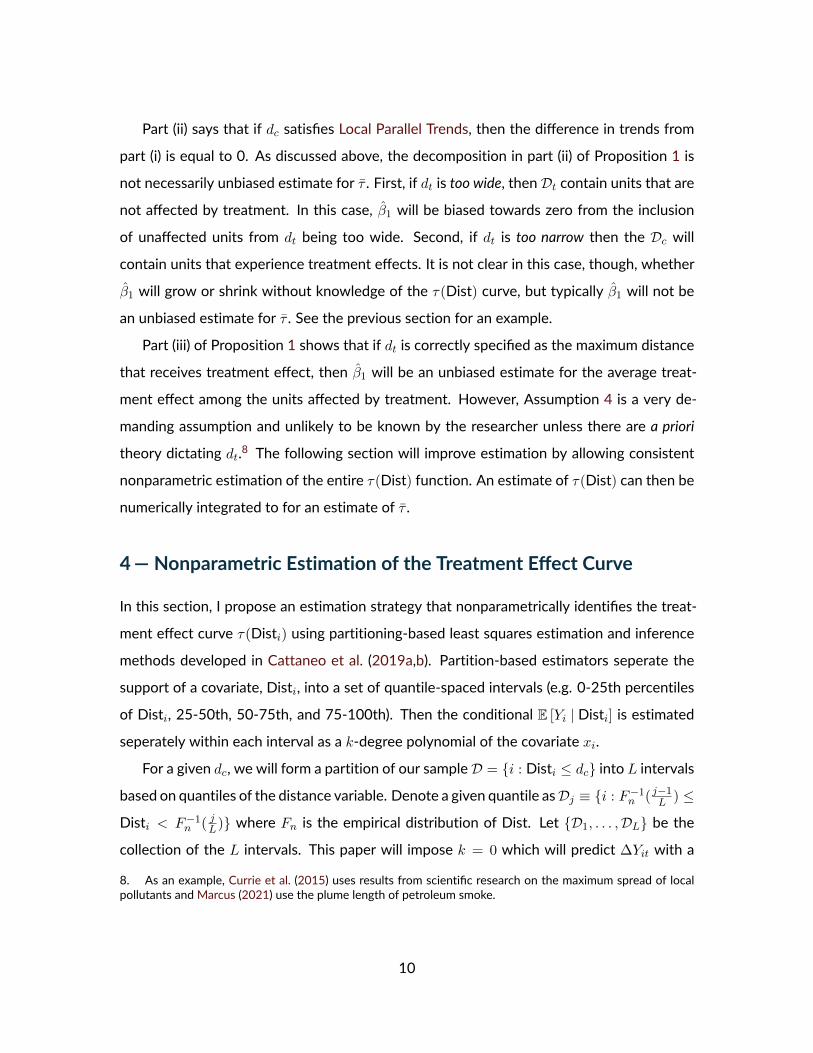
Part (ii) says that if dc satisfies Local Parallel Trends, then the difference in trends frompart (i) is equal to 0. As discussed above, the decomposition in part (ii) of Proposition 1 isnot necessarily unbiased estimate for τ . First, if dt is too wide, then Dt contain units that arenot affected by treatment. In this case, β1 will be biased towards zero from the inclusionof unaffected units from dt being too wide. Second, if dt is too narrow then the Dc willcontain units that experience treatment effects. It is not clear in this case, though, whetherβ1 will grow or shrink without knowledge of the τ(Dist) curve, but typically β1 will not bean unbiased estimate for τ . See the previous section for an example.

Part (iii) of Proposition 1 shows that if dt is correctly specified as the maximum distancethat receives treatment effect, then β1 will be an unbiased estimate for the average treat-ment effect among the units affected by treatment. However, Assumption 4 is a very de-manding assumption and unlikely to be known by the researcher unless there are a priori

theory dictating dt.8 The following section will improve estimation by allowing consistentnonparametric estimation of the entire τ(Dist) function. An estimate of τ(Dist) can then benumerically integrated to for an estimate of τ .

4— Nonparametric Estimation of the Treatment Effect Curve

In this section, I propose an estimation strategy that nonparametrically identifies the treat-ment effect curve τ(Disti) using partitioning-based least squares estimation and inferencemethods developed in Cattaneo et al. (2019a,b). Partition-based estimators seperate thesupport of a covariate, Disti, into a set of quantile-spaced intervals (e.g. 0-25th percentilesof Disti, 25-50th, 50-75th, and 75-100th). Then the conditional E [Yi | Disti] is estimatedseperately within each interval as a k-degree polynomial of the covariate xi.

For a given dc, we will form a partition of our sampleD = {i : Disti ≤ dc} into L intervalsbased on quantiles of the distance variable. Denote a given quantile asDj ≡ {i : F−1n ( j−1L ) ≤

Disti < F−1n ( jL)} where Fn is the empirical distribution of Dist. Let {D1, . . . ,DL} be the

collection of the L intervals. This paper will impose k = 0 which will predict ∆Yit with a8. As an example, Currie et al. (2015) uses results from scientific research on the maximum spread of localpollutants and Marcus (2021) use the plume length of petroleum smoke.

10

constant within each interval.9These averages are defined as

∆Y j ≡1

nj

∑i∈Dj

∆Yit,

where the number of units in bin Dj is nj ≈ n/L. Our estimator for E [∆Yit | Disti] is thengiven by

∆Yit =

L∑j=1

1i∈Dj∆Y j

As the number of intervals approach infinity, this estimatewill approachE [∆Yit | Dist = d] inamean-squared error sense. Under Local Parallel Trends,E [∆Yit | Dist = d] ≡ E [τ(Dist) | Dist = d]+

λ. To remove λ, we require a less-strict version of assumption 4.Assumption 5 (dt is within dc). A distance dc satisfies this assumption if there exists a dis-tance dt with 0 < dt < dc such that (i) Assumption 4 holds and (ii) F (dc)− F (dt) > 0.

If a distance dc satisfies Local Parallel Trends and (5), the mean within the last ringDk willestimate λ as the number of bins L → ∞. The reason for this is simple, as L → ∞, the lastbin will have the left end-point > dt and therefore τ(Dist) = 0 in DL. Under local paralleltrends, the last ring will therefore estimate λ. Therefore, estimates of τ(Disti) can be formedfor each interval as τj ≡ ∆Y j −∆Y L.Proposition 2 (Consistency of Nonparametric Estimator). Given that units follow model (2)and dc satisfies Local Parallel Trends and assumption (5), as n and L→∞

τ ≡L∑i=1

τj1i∈Dj →unif τ(Dist)

where dj corresponds to the F−1(Dj).As discussed in Section 2, specifying dt correctly is important to identify the average

9. Approximation can bemade arbitrarily close to the true conditional expectation function by either increasingthe number of intervals or by increasing the polynomial order to infinity, so setting k = 0 does not impose anycost.

11

treatment effect among the affected in the parametric estimator. The nonparametric esti-mator only requires that treatment effects become zero before dc, i.e. that such a dt exists.However, the estimatorwould no longer identify the treatment effect curve under themilderAverage Parallel Trends assumption. Therefore, a researcher should justify explicity the as-sumption that, within the dc ring, every unit is subject to the same trend. This is most likelyto be satisfied on a very local level and not very plausible in the case of larger units, e.g.counties.

The nonparametric approach allows estimation of the treatment effect curve whereasthe indicator approach, at best, can only estimate an average effect among units experiencingeffects. The treatment effect curve allows researcher to understand differences in treatmenteffect across distance. For example, typically one would assume treatment effects shrinkover distance and evidence of this from the nonparametric approach can strengthen a causalclaim. In some cases, such as a negative hyper-local shock and a postivie local shock (e.g. alocal bus-stop), the treatment effect can even change sign across distances. In this case, theaverage effect could be near zero even though there are significant effects occuring.

Plotting estimates τj can provide visual evidence for the underlying Local Parallel Trendsassumption. Typically, treatment effect will stop being experienced far enough away fromdc that some estimates of τj with j ‘close to’ L will provide informal tests for parallel trendsholding. Figure 4 provide an examplewhere plotting of τj provide strong evidence in supportof local parallel trends as it appears that after some distance, average effects are consistetlycentered around zero. This is not a formal test as it could be the case that the true treatmenteffect curve, τ(Dist) is perfectly cancelling out with the counterfactual trends curve λ(Dist)producing near zero estimates, but this is a knive’s edge case.

The above proposition shows that the series estimator will consistenly estimate the treat-ment effect curve, τ(Dist) as the number of binsL and the number of observations n both goto infinity. In finite-samples though, wewill have a fixedL and hence a fixed set of treatmenteffect estimates {τ1, . . . , τL} with τL ≡ 0 by definition. The estimates τj are approximatelyequal to E [τ(Dist) | Dist ∈ Dj ] or the average treatment effect within the interval Dj .

The choice of L in finite samples is not entirely clear. Cattaneo et al. (2019a) derivethe IMSE-optimal choice of L which is a completely data-driven choice. The optimal L is

12

driven by two competing terms in the IMSE formula. On the one hand, as L increases, theconditional expectation function is allowed to vary more across values of Dist and hencebias of the estimator decreases. However, larger values of L increase the variance of theestimator. Balancing this trade-off depends on the shape and curvature of τ(Dist). Theresulting choice of L∗ and the use of quantiles of the data allows a completely data-drivenchoice of the number of rings and their endpoints which allows for estimation in a principledand objective way. This principled estimator removes researcher-incentives to search acrosschoices of rings to provide the best evidence.

For a given L∗, Cattaneo et al. (2019a) show the large-sample asymptotics of the esti-mates ∆Y j and provide robust standard errors for the conditional means that account forthe additional randomness due to quantile estimation. Since our estimator is a difference inmeans, standard errors on our estimate τj are given by√σ2j + σ2L, where σj is the standarderror recommended by Cattaneo et al. (2019a). These standard errors are produced by theStata/R package binsreg. Inference can be done by using the estimated t-stat with the stan-dard normal distribution. There may be concerned that the standard errors need to adjustfor spatial correlation. However, this is not the case under assumption (2) as this implies theerror term is uncorrelated with distance.

5— Application to Neighborhood Effects of Crime Risk

To highlight the advantages of my proposed estimator, I revisit the analysis of Linden andRockoff (2008). This paper analyzes the effect of a sex offender moving to a neighborhoodon home prices. This paper uses the ring method with treated homes being defined as beingwithin 1/10th of the sex offender’s home and the control units being between 1/10th and1/3rd of a mile from the home. The authors make a case for the ring method by arguing thatwithin a neighborhood, Local Parallel Trends holds since they are looking in such a narrowarea and purchasing a home is difficult to be precisely located with concurrent hyper-localshocks.

As for the choice of the treatment ring, there is little a priori reasons to know how far theeffects of sex offender arrival will extend in the neighborhood. The authors provide graph-

13

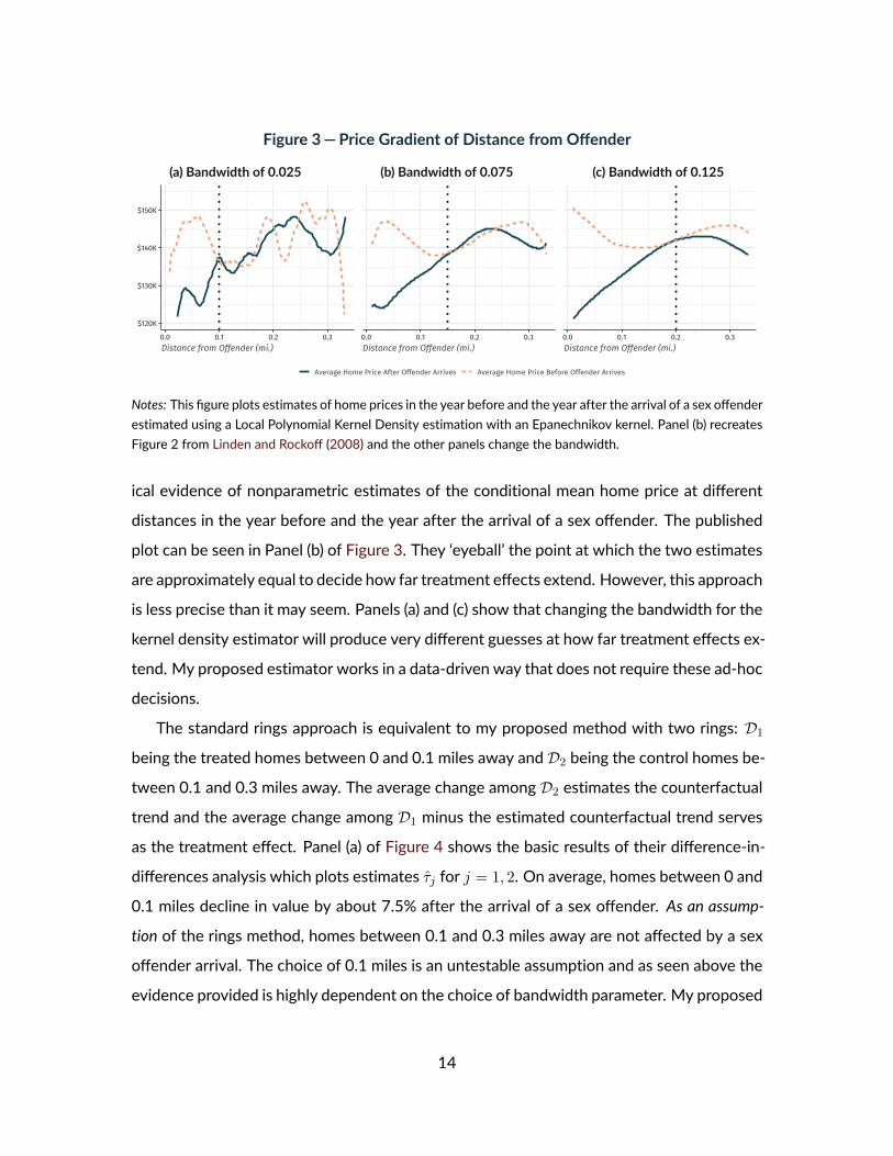
Figure 3—Price Gradient of Distance from Offender

(a) Bandwidth of 0.025 (b) Bandwidth of 0.075 (c) Bandwidth of 0.125

Notes: This figure plots estimates of home prices in the year before and the year after the arrival of a sex offenderestimated using a Local Polynomial Kernel Density estimation with an Epanechnikov kernel. Panel (b) recreatesFigure 2 from Linden and Rockoff (2008) and the other panels change the bandwidth.

ical evidence of nonparametric estimates of the conditional mean home price at differentdistances in the year before and the year after the arrival of a sex offender. The publishedplot can be seen in Panel (b) of Figure 3. They ‘eyeball’ the point at which the two estimatesare approximately equal to decide how far treatment effects extend. However, this approachis less precise than it may seem. Panels (a) and (c) show that changing the bandwidth for thekernel density estimator will produce very different guesses at how far treatment effects ex-tend. My proposed estimator works in a data-driven way that does not require these ad-hocdecisions.

The standard rings approach is equivalent to my proposed method with two rings: D1

being the treated homes between 0 and 0.1 miles away and D2 being the control homes be-tween 0.1 and 0.3 miles away. The average change among D2 estimates the counterfactualtrend and the average change among D1 minus the estimated counterfactual trend servesas the treatment effect. Panel (a) of Figure 4 shows the basic results of their difference-in-differences analysis which plots estimates τj for j = 1, 2. On average, homes between 0 and0.1 miles decline in value by about 7.5% after the arrival of a sex offender. As an assump-

tion of the rings method, homes between 0.1 and 0.3 miles away are not affected by a sexoffender arrival. The choice of 0.1 miles is an untestable assumption and as seen above theevidence provided is highly dependent on the choice of bandwidth parameter. My proposed

14

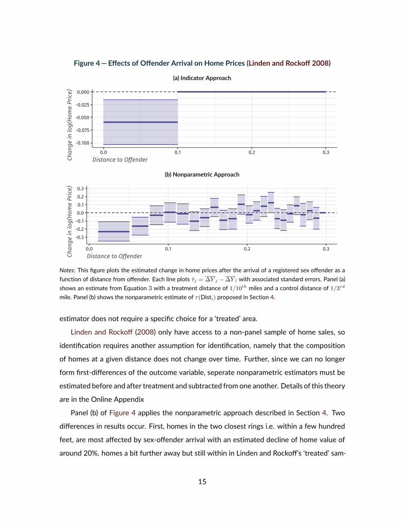
Figure 4—Effects of Offender Arrival on Home Prices (Linden and Rockoff 2008)

(a) Indicator Approach

(b) Nonparametric Approach

Notes: This figure plots the estimated change in home prices after the arrival of a registered sex offender as afunction of distance from offender. Each line plots τj = ∆Y j − ∆Y l with associated standard errors. Panel (a)shows an estimate from Equation 3 with a treatment distance of 1/10th miles and a control distance of 1/3rd

mile. Panel (b) shows the nonparametric estimate of τ(Disti) proposed in Section 4.

estimator does not require a specific choice for a ‘treated’ area.Linden and Rockoff (2008) only have access to a non-panel sample of home sales, so

identification requires another assumption for identification, namely that the compositionof homes at a given distance does not change over time. Further, since we can no longerform first-differences of the outcome variable, seperate nonparametric estimators must beestimated before and after treatment and subtracted fromone another. Details of this theoryare in the Online Appendix

Panel (b) of Figure 4 applies the nonparametric approach described in Section 4. Twodifferences in results occur. First, homes in the two closest rings i.e. within a few hundredfeet, are most affected by sex-offender arrival with an estimated decline of home value ofaround 20%. homes a bit further away but still within in Linden and Rockoff’s ‘treated’ sam-

15

ple do not experience statistically significant treatment effects. As discussed above, Lindenand Rockoff’s estimate of τ is attenuated towards zero because of the inclusion of homeswith little to no treatment effects, leading them to understate the effect of arrival on homeprices. The nonparametric approach improves on answering this question by providing amore complete picture of the treatment effect curve. The magnitude of treatment effectsdecrease over distance, providing additional evidence that the arrival causes a drop in homeprices.10

The second advantage of this approach is that the produced figure provides an informaltest of the local parallel trends assumption. After 0.1 miles, the estimated treatment effectcurve becomes centered at zero consistently. This implies that units within each ring havethe same estimated trend as the outer most ring, providing suggestive evidence that homesin this neighborhood are subject to the same trends.

6— Discussion

This article formalizes a common applied identification strategy that has a strong intuitiveappeal. When treatment effects of shocks are experienced in only part of an area thatwould otherwise be on a common neighborhood-trend, difference-in-differences compar-isons within a neighborhood can identify treatment effects. However, this paper shows thatthe typical estimator for treatment effects requires a very strong assumption and returnsonly an average treatment effect among affected units when this assumption holds.

This article then proposes an improved estimator that relies on nonparametric seriesestimators. The nonparametric estimator allows for estimation of the treatment effect atdifferent distances from treatment, similar to a dose-response function, which can allowbetter understanding of who is experiencing effects and how this changes across ‘exposure’to a shock. More, in some cases it can provide explanation for null results. For example,if a bus station creates negative externalities for apartments that border the station butpositive externalities for apartments within walking distance, the average effect could bezero. However, nonparametric estimation would reveal the two effects seperately.

10. This is similar to estimating a dose-response function as evidence supporting a causal mechanism.16

References

Alexander, Diane, Janet Currie, and Molly Schnell. 2019. “Check up before you check out:Retail clinics and emergency room use.” Journal of Public Economics 178 104050. 10.1016/

j.jpubeco.2019.104050.Aronow, Peter M., Dean Eckles, Cyrus Samii, and Stephanie Zonszein. 2020. “SpilloverEffects in Experimental Data.” arXiv:2001.05444 [cs, stat], http://arxiv.org/abs/2001.05444, arXiv: 2001.05444.

Aronow, Peter M., Cyrus Samii, and Ye Wang. 2021. “Design-Based Inference for SpatialExperiments with Interference.” arXiv:2010.13599 [math, stat], http://arxiv.org/abs/2010.13599, arXiv: 2010.13599.

Asquith, Brian J., EvanMast, and Davin Reed. 2021. “Local Effects of Large New ApartmentBuildings in Low-Income Areas.” The Review of Economics and Statistics 1–46. 10.1162/

rest_a_01055.Berg, Tobias, and Daniel Streitz. 2019. Handling Spillover Effects in Empirical Research. Work-ing Paper, 59.

Billings, Stephen B. 2011. “Estimating the value of a new transit option.” Regional Scienceand Urban Economics 41 (6): 525–536. 10.1016/j.regsciurbeco.2011.03.013.

Butts, Kyle. 2021. “Difference-in-Differences Estimation with Spatial Spillovers.”Campbell, John Y, Stefano Giglio, and Parag Pathak. 2011. “Forced Sales and House Prices.”American Economic Review 101 (5): 2108–2131. 10.1257/aer.101.5.2108.

Casey, Marcus, Jeffrey C. Schiman, and Maciej Wachala. 2018. “Local Violence, AcademicPerformance, and School Accountability.” AEA Papers and Proceedings 108 213–216. 10.

1257/pandp.20181109.

17

Cattaneo, Matias D., Richard K. Crump, Max H. Farrell, and Yingjie Feng. 2019a. “OnBinscatter.” arXiv:1902.09608 [econ, stat], http://arxiv.org/abs/1902.09608, arXiv:1902.09608.

Cattaneo, Matias D., Max H. Farrell, and Yingjie Feng. 2019b. “Large Sample Properties ofPartitioning-Based Series Estimators.” arXiv:1804.04916 [econ, math, stat], http://arxiv.org/abs/1804.04916, arXiv: 1804.04916.

Clarke, Damian. 2017. “Estimating Difference-in-Differences in the Presence of Spillovers.”Munich Personal RePEc Archive 52.

Cui, Lin, and Randall Walsh. 2015. “Foreclosure, vacancy and crime.” Journal of Urban Eco-

nomics 87 72–84. 10.1016/j.jue.2015.01.001.Currie, Janet, Lucas Davis, Michael Greenstone, and Reed Walker. 2015. “EnvironmentalHealth Risks andHousing Values: Evidence from1,600 Toxic PlantOpenings andClosings.”American Economic Review 105 (2): 678–709. 10.1257/aer.20121656.

Delgado, Michael S., and Raymond J.G.M. Florax. 2015. “Difference-in-differences tech-niques for spatial data: Local autocorrelation and spatial interaction.” Economics Letters137 123–126. 10.1016/j.econlet.2015.10.035.

Di Tella, Rafael, and Ernesto Schargrodsky. 2004. “Do Police Reduce Crime? Estimates Usingthe Allocation of Police Forces After a Terrorist Attack.” American Economic Review 94 (1):115–133. 10.1257/000282804322970733.

Diamond, Rebecca, and Tim McQuade. 2019. “Who Wants Affordable Housing in TheirBackyard? An Equilibrium Analysis of Low-Income Property Development.” journal of po-litical economy 55.

Gerardi, Kristopher, Eric Rosenblatt, Paul S. Willen, and Vincent Yao. 2015. “Foreclosureexternalities: New evidence.” Journal of Urban Economics 87 42–56. 10.1016/j.jue.2015.02.

004.Gibbons, Stephen, and Stephen Machin. 2005. “Valuing rail access using transport innova-tions.” Journal of Urban Economics 57 (1): 148–169. 10.1016/j.jue.2004.10.002.

18

Linden, Leigh, and Jonah E Rockoff. 2008. “Estimates of the Impact of Crime Risk onProperty Values from Megan’s Laws.” American Economic Review 98 (3): 1103–1127.10.1257/aer.98.3.1103.

Marcus, Michelle. 2021. “Going Beneath the Surface: Petroleum Pollution, Regulation, andHealth.” American Economic Journal: Applied Economics 13 (1): 72–104. 10.1257/app.

20190130.Sullivan, Daniel M. 2017. The True Cost of Air Pollution: Evidence from the Housing Market.Working Paper.

Verbitsky-Savitz, Natalya, and Stephen W. Raudenbush. 2012. “Causal Inference Under In-terference in Spatial Settings: A Case Study Evaluating Community Policing Program inChicago.” Epidemiologic Methods 1 (1): . 10.1515/2161-962X.1020.

A— Proofs

A.1. Proof of Proposition 1

Proof. Note using our model (2), we have

E[β1

]= E [∆Yit | Dt]− E [∆Yit | Dc]

= E [τ(Disti) + λ(Disti) + ∆εi | Dt]− E [τ(Disti) + λ(Disti) + ∆εi | Dc]

= E [τ(Disti) | Dt]− E [τ(Disti) | Dc] + E [λ(Disti) | Dt]− E [λ(Disti) | Dc] + E [∆εi | Dt]− E [∆εi | Dc] .

By construction, ∆εi is uncorrelated with distance, so the final two terms in the sum is zerogiving us result (i). Result (ii) comes from the fact that within dc, λ(Disti) = λ. Result (iii)comes from the fact that if dt is the correct cutoff E [τ(Disti) | Dc] = 0.A.2. Proof of Proposition 2

Proof. Note that L → ∞ implies dt ≤ F−1n (L−1L ) by assumption (5). This implies ∆Y L →p λ

as n→∞ by assumption (5).

19

From assumption (2) and from our model (2), we have

τj = ∆Y j −∆Y L

→p E [τ(Dist) | Dist ∈ Dj ] + λ− λ

= E [τ(Dist) | Dist ∈ Dj ]

As L → ∞ and n → ∞, we have that Dj approaches a set containing a singular point,say dj . Therefore

τj →p E [τ(Dist) | Dist = dj ]

The sum of τj therefore approach the conditional expectation function of τ(Dist) point-wisely. See Cattaneo et al. (2019b) for proof of uniform convergence and underlying smooth-ness conditions for nonparametric consistency.

B— Repeated Cross-Sectional Data

In the case of repeated cross-sectional data, we have individuals i that appear in the data inperiod t(i) ∈ {0, 1}. However, since we no longer are able to observe units in both periods,we are not able to take first differences. Our model therefore will have a λ term for bothperiods. Therefore, λ includes the average of µi, covariates, and period shocks at a givendistance.

Yi = τ(Disti)1t(i)=1 + λt(i)(Disti) + νit. (4)The parallel trends assumption must be modified now in the case of cross sections:

Assumption 6 (Local Parallel Trends (RC)). For a distance d, we say that ‘local parallel trends’hold if for all positive d, d′ ≤ d, then λ1(d)− λ0(d) = λ1(d

′)− λ0(d′).Assumption 7 (Average Parallel Trends (RC)). For a pair of distances dt and dc, we say that‘average parallel trends’ hold ifE [λ1(d) | 0 ≤ d ≤ dt]−E [λ0(d) | 0 ≤ d ≤ dt] = E [λ1(d) | dt < d ≤ dc]−

E [λ0(d) | dt < d ≤ dc].

20

The parallel trends assumption is a bit more complicated now and is theoretically stricter.Local Parallel Trends (RC) still require changes in outcomes over time for a given unit i mustbe constant across distance (or on average in the case of Average Parallel Trends (RC)). How-ever since the composition of units can change over time, this also requires that the averageof individual fixed effects must be constant across time. This is well understood in the he-donic pricing literature that the composition of homes being sold can not change over timefor identification (e.g. Linden and Rockoff (2008)).

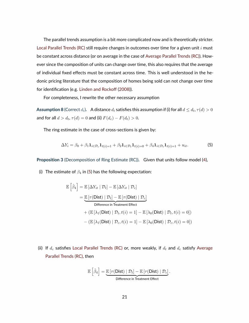
For completeness, I rewrite the other necessary assumptionAssumption 8 (Correct dt). A distance dt satisfies this assumption if (i) for all d ≤ dt, τ(d) > 0

and for all d > dt, τ(d) = 0 and (ii) F (dc)− F (dt) > 0.The ring estimate in the case of cross-sections is given by:

∆Yi = β0 + β11i∈Dc1t(i)=1 + β21i∈Dt1t(i)=0 + β41i∈Dt1t(i)=1 + uit. (5)

Proposition 3 (Decomposition of Ring Estimate (RC)). Given that units follow model (4),(i) The estimate of β4 in (5) has the following expectation:

E[β4

]= E [∆Yit | Dt]− E [∆Yit | Dc]

= E [τ(Dist) | Dt]− E [τ(Dist) | Dc]︸ ︷︷ ︸Difference in Treatment Effect+ (E [λ1(Dist) | Dt, t(i) = 1]− E [λ0(Dist) | Dt, t(i) = 0])

− (E [λ1(Dist) | Dc, t(i) = 1]− E [λ0(Dist) | Dc, t(i) = 0])

(ii) If dc satisfies Local Parallel Trends (RC) or, more weakly, if dt and dc satisfy AverageParallel Trends (RC), then

E[β4

]= E [τ(Dist) | Dt]− E [τ(Dist) | Dc]︸ ︷︷ ︸Difference in Treatment Effect

.

21

(iii) If dc satisfies Local Parallel Trends (RC) and dt satisfies Assumption 8, then

E[β4

]= τ .

Proof. With some algebraic manipulation, we can rewrite our difference-in-differences esti-mator as

(E [Yi | Dt, t(i) = 1]− E [Yi | Dt, t(i) = 0])− (E [Yi | Dc, t(i) = 1]− E [Yi | Dc, t(i) = 0]))

= (E [τ(Disti) + λ1(Disti) + νi1 | Dt, t(i) = 1]− E [λ0(Disti) + νi0 | Dt, t(i) = 0])

− (E [τ(Disti) + λ1(Disti) + νi1 | Dc, t(i) = 1]− E [λ0(Disti) + νi0 | Dc, t(i) = 0])

= E [τ(Disti) | Dt, t(i) = 1]− E [τ(Disti) | Dc, t(i) = 0] +

(E [λ1(Disti) | Dt, t(i) = 1]− E [λ0(Disti) | Dt, t(i) = 0])

− (E [λ1(Disti) | Dc, t(i) = 1]− E [λ0(Disti) | Dc, t(i) = 0]) ,

where the terms consisting of νit cancel out as they are uncorrelated with distance. Propo-sitions (ii) and (iii) follow the same arguments as in the panel case.

Part (i) of this theorem shows that under no parallel trends assumption, the ‘Differencein Trends’ term becomes the change in λt for the treated ring minus the change in for thecontrol ring. As discussed above, this change in lambdas can be do to period specific shocksor changes in the composition of units observed in each period.B.1. Nonparametric Estimation

Since we can no longer perform a single nonparmaetric regression on first differences inthe context of cross-sections, our nonparametric estimator must be adjusted. The modifiedprocedure will fit a nonparametric estimate of E [Yi | Disti, t] seperately for t = 0 and t = 1

with a restriction that the bin intervals {D1, . . . ,DL} must be the same in both samples.11Then, for each distance bin we calculate an estimate of Yj,t which corresponds to the sampleaverage of observations in period t in bin Dj .11. The number of intervals are decided based on a different IMSE condition described in Cattaneo et al. (2019a)and the quantiles are calculated using the distribution of distances in both periods.

22

Then estimates of τj can be formed as

τj =[Yj,1 − Yj,0

]−[YL,1 − YL,0

],

where, as before, the change in trends in the last ring serve as an estimate for the counterfac-tual trend. Under Local Parallel Trends (RC), estimates of ˆtauj are consistent forE [τ(Disti) | i ∈ Dj ]

and the treatment effect curve converges uniformly to the treatment effect curve τ(d).Standard errors are formed similarly as before, but is the difference of four means so

they can be formed as√σ2j,1 + σ2j,0 + σ2L,1 + σ2L,0. These individual estimates and standarderrors can be produced by the Stata/R package binsreg.

23