Diet Analysis and Assessment of Habitat and Prey ...

DIET ANALYSIS AND ASSESSMENT OF HABITAT AND PREY AVAILABILITY

ASSOCIATED WITH TEXAS DIAMOND-BACKED TERRAPIN (MALACLEMYS TERRAPIN

LITTORALIS)

by

Bryan J. Alleman, B.S.

THESIS

Presented to the Faculty of

The University of Houston- Clear Lake

In Partial Fulfillment

of the Requirements

for the Degree

MASTER OF SCIENCE

THE UNIVERSITY OF HOUSTON- CLEAR LAKE

Fall 2015


ASSOCIATED WITH TEXAS DIAMOND-BACKED TERRAPIN (MALACLEMYS TERRAPIN

LITTORALIS)

by

Bryan J. Alleman

APPROVED BY

_________________________________________________

George Guillen, Ph.D., Chair

_________________________________________________

Richard Puzdrowski, Ph.D., Committee Member

_________________________________________________

Cynthia Howard, Ph.D., Committee Member

_________________________________________________

Ju H. Kim, Ph. D., Associate Dean

_________________________________________________

Zbigniew J. Czajkiewicz,, Ph.D., Dean

DEDICATION

For my grandmother, Yvonne Alleman (1934-1994).

Thanks for fostering and encouraging my curiosity of the natural world at a young age, and

starting me on my path.

ACKNOWLEDGEMENTS

I would like to thank Texas Parks and Wildlife Department for funding that supported my

project. Also, the Environmental Institute of Houston (EIH) for additional support and

assistance. Specifically, I would like to thank all EIH staff and students that contributed to

the development of the study. I am grateful to Dr. George Guillen, Jenny Oakley, Mandi

Gordon, Rachel George, and Emma Clarkson for guidance, logistical support, and data

collection during numerous, long field days.

I would also like to thank James and Denise Alleman, Ashley King, Nancy Christensen, and

the rest of my family for the continued support and encouragement I receive from them.

Thank you all very much.

v

ABSTRACT


ASSOCIATED WITH TEXAS DIAMOND-BACKED TERRAPIN (MALACLEMYS

TERRAPIN LITTORALIS)

Bryan J. Alleman, M.S.

The University of Houston – Clear Lake

Thesis Chair: Dr. George Guillen

The Diamond-backed Terrapin (Malaclemys terrapin) is a species of turtle specialized for

living in brackish and saltmarsh environments, and due to diet is likely a keystone predator.

The Texas Diamond-backed Terrapin (M. t. littoralis) is the subspecies found along most of

the Texas Gulf Coast. Past studies have been conducted on the diet and prey of the Atlantic

subspecies of Diamond-backed Terrapin. Previous studies indicate a diet primarily consisting

of various crustacean and mollusk species with variations along their range. Due to body size

sexual dimorphism, studies also show differences in diet between males and females. There

is currently a paucity of data on the diet of this species along the coast of the Gulf of Mexico,

and specifically on the Texas Gulf Coast. This study examined the prey availability and diet

of the Texas Diamond-backed Terrapin. Dietary analysis via fecal analysis indicated

Gastropoda and Decapoda as major components to Texas terrapin diet. The remains of

vi

plicate horn snails (Cerithidea pliculosa) and fiddler crabs (Uca spp.) were the most common

prey items found in all samples. There were significant differences between the diet of male

and female terrapin, specifically in amounts and proportion of periwinkle snails (Littorina

irrorata), blue crabs (Callinectes sapidus), total Gastropods, and total Decapods consumed.

Female terrapin consumed more L. irrorata and total Gastropods than males, while males

were found to consume more C. sapidus and total Decapods than females. Males also

demonstrated higher dietary diversity. Significant seasonal differences in diet were detected

between seasons for total Gastropods, C. sapidus, and Uca spp. Additional dietary

differences were detected for less common dietary components.

Randomly selected sites lacking terrapin exhibited a significantly higher number of

plant species and vegetation coverage when compared to terrapin capture locations. No

significant difference in the coverage of dominant plant species Spartina alterniflora was

detected at terrapin capture versus non-capture sites. Randomly selected sites lacking terrapin

had significantly higher numbers of Uca spp. burrows than capture locations. Multiple

significant seasonal and location differences in vegetation and prey were detected at capture

sites. However, no differences for any prey or habitat factor were detected between sexes at

capture locations. Results from fecal analysis indicate a slightly different diet for terrapin

than previously reported in other studies. However, habitat and prey availability findings

support previous studies. The combined results extend the basic knowledge and

understanding of diet and habitat utilization by this species which will be useful for ongoing

conservation and management of M. terrapin, especially the Texas subspecies.

vii

TABLE OF CONTENTS

ACKNOWLEDGEMENTS ............................................................................................... iv

ABSTRACT ........................................................................................................................ v

TABLE OF CONTENTS .................................................................................................. vii

LIST OF TABLES ............................................................................................................. ix

TABLE OF FIGURES ........................................................................................................ x

INTRODUCTION .............................................................................................................. 1

Life History ..................................................................................................................... 1

Terrapin Diet ................................................................................................................... 2

Prey Availability ............................................................................................................. 5

Objectives and Hypotheses ............................................................................................. 5

METHODS ......................................................................................................................... 6

Study Site ........................................................................................................................ 6

Terrapin Capture ........................................................................................................... 11

Prey Availability ........................................................................................................... 12

Fecal Collection............................................................................................................. 15

Data Analysis ................................................................................................................ 19

RESULTS ......................................................................................................................... 21

Prey Availability and Habitat ........................................................................................ 21

Habitat Quadrats at Random versus Capture Locations ........................................... 23

Habitat Quadrats by Season at Capture Locations .................................................... 28

Habitat Quadrats by Marsh Site at Capture Locations.............................................. 30

Habitat and Temperature........................................................................................... 34

Prey Quadrats at Random versus Capture Locations ................................................ 38

Prey Quadrats by Season at Capture Locations ........................................................ 39

Prey Quadrats by Marsh Site .................................................................................... 41

Fecal Analysis ............................................................................................................... 44

Diversity Indices ....................................................................................................... 46

viii

Frequency of Occurrence .......................................................................................... 47

Gravimetric Analysis ................................................................................................ 50

Volumetric Analysis ................................................................................................. 61

Volumetric vs. Gravimetric ...................................................................................... 72

DISCUSSION ................................................................................................................... 73

Effects of Habitat on Terrapin Distribution .................................................................. 73

Effects of Prey Availability on Terrapin Distribution ................................................... 77

Terrapin Diet Analyses.................................................................................................. 79

Dietary Analysis Techniques ........................................................................................ 87

Future Work .................................................................................................................. 87

CONCLUSIONS............................................................................................................... 90

LITERATURE CITED ..................................................................................................... 92

ix

LIST OF TABLES

Table 1. Number of prey quadrats collected by season. ................................................... 23

Table 2. Number of fecal samples collected by season. ................................................... 45

Table 3. Shannon-Weiner (H'), Shannon Evenness (E), and Berger-Parker (BPI) indices

of diversity for M. t. littoralis diet .................................................................................... 47

Table 4. Frequency of occurrence of prey items found in terrapin fecal samples ............ 48

Table 5. Percentages of prey items by weight (g) found in terrapin fecal samples .......... 51

Table 6. Percentages of prey items by volume (mL) found in terrapin fecal samples ..... 62

x

TABLE OF FIGURES

Figure 1. Imagery indicating surveyed sites along Texas Gulf Coast. ............................... 7

Figure 2. An aerial image that shows West Galveston Bay, Texas sites. ........................... 7

Figure 3. An aerial image that shows the Matagorda Bay, Texas site. ............................. 10

Figure 4. An aerial image that shows Texas Point National Wildlife Refuge. ................. 10

Figure 5. Image indicating location of Sweetwater Lake study site in relation to South

Deer Island and Sportsman Road. ..................................................................................... 11

Figure 6. The 1-m2

quadrat used in the field. .................................................................... 13

Figure 7. Photograph showing measure of Littorina length. ............................................ 13

Figure 8. Photograph showing measure of Littorina width. ............................................. 14

Figure 9. Female Diamond-backed Terrapin in storage bin during fecal collection. ....... 16

Figure 10. Fecal remains on 0.5mm sieve after being poured from collection bin. ......... 16

Figure 11. Two vials containing fecal samples and preservative. .................................... 17

Figure 12. Aluminum container and fecal sample used during drying and weighing. ..... 17

Figure 13. Graduated cylinder (25mL) containing partial fecal sample and water. ......... 19

Figure 14. Percentage of 1 m2 quadrats with listed species as the dominant plant species

at random (n = 78) and capture (n = 215) locations. ......................................................... 22

Figure 15. Percentage of 1 m2 quadrats with listed vegetation heights at random (n = 78)

and capture (n = 215) locations. ........................................................................................ 23

Figure 16. Boxplot depicting location differences of number of plant species in 1 m2 prey

quadrats ............................................................................................................................. 24

Figure 17. Histogram depicting percentage of prey quadrats from random (n = 78) and

capture (n = 215) locations containing a given number of plant species. ......................... 25

Figure 18. Boxplot depicting location differences of vegetation height in 1 m2 prey

quadrats ............................................................................................................................. 25

Figure 19. Boxplot depicting location differences of vegetation cover percentage in 1 m2

prey quadrats ..................................................................................................................... 26

Figure 20. Boxplot depicting location differences of Batis maritima coverage percentage

in 1 m2 prey quadrats. ....................................................................................................... 26

Figure 21. Boxplot depicting location differences of Salicornia spp. coverage percentage


Figure 22. Boxplot depicting location differences of Spartina alterniflora coverage

percentage in 1 m2 prey quadrats ...................................................................................... 27

xi

Figure 23. Boxplot depicting seasonal differences of Spartina alterniflora coverage at

terrapin capture locations in 1 m2 prey quadrats. .............................................................. 29

Figure 24. Boxplot depicting seasonal differences of Batis maritima coverage at terrapin

capture locations in 1 m2 prey quadrats ............................................................................ 29

Figure 25. Boxplot depicting seasonal differences of Salicornia spp. coverage at terrapin

capture locations in 1 m2 prey quadrats ............................................................................ 30

Figure 26. Boxplot depicting marsh differences at capture locations of vegetation height


Figure 27. Boxplot depicting marsh differences at capture locations of number of plant

species in 1 m2 prey quadrats ............................................................................................ 32

Figure 28. Boxplot depicting marsh differences at capture locations of vegetation

coverage in 1 m2 prey quadrats. ........................................................................................ 33

Figure 29. Boxplot depicting marsh differences at capture locations of Batis maritima

coverage in 1 m2 prey quadrats ......................................................................................... 33

Figure 30. Boxplot depicting marsh differences at capture locations of Spartina patens

coverage in 1 m2 prey quadrats ......................................................................................... 34

Figure 31. Boxplot depicting median temperatures at breast height (26.25 °C) and ground

level (27. 00 °C) at both random and capture locations. Significant difference between

median values.................................................................................................................... 35

Figure 32. Boxplot depicting location differences of air temperature at ground level

recorded at 1 m2 prey quadrats.......................................................................................... 36

Figure 33. Boxplot depicting vegetation height differences in air temperature at ground

level recorded at 1 m2 prey quadrats at terrapin capture locations ................................... 37

Figure 34. Boxplot depicting dominant vegetation differences in air temperature at

ground level recorded at 1 m2 prey quadrats at terrapin capture locations. ...................... 37

Figure 35. Boxplot depicting fiddler crab (Uca spp.) burrow number differences between

random and terrapin capture locations in 1 m2 prey quadrats ........................................... 38

Figure 36. Boxplot depicting Littorina irrorata number differences between random and

terrapin capture locations in 1 m2 prey quadrats. .............................................................. 39

Figure 37. Boxplot depicting seasonal differences of Uca spp. burrows at terrapin capture

locations in 1 m2 prey quadrats ......................................................................................... 40

Figure 38. Boxplot depicting seasonal differences of Littorina irrorata at terrapin capture

locations in 1 m2 prey quadrats ......................................................................................... 40

Figure 39. Boxplot depicting marsh differences at capture locations of Uca burrow

numbers in 1 m2 prey quadrats.......................................................................................... 42

Figure 40. Boxplot depicting marsh differences at capture locations of Littorina irrorata

numbers in 1 m2 prey quadrats.......................................................................................... 42

Figure 41. Marsh differences at capture locations of Cerithidea pliculosa presence in 1

m2 prey quadrats ............................................................................................................... 43

xii

Figure 42. Marsh differences at capture locations of presence of other potential prey

items in 1 m2 prey quadrats ............................................................................................... 43

Figure 43. Boxplots depicting total sample volume (mL) and weight (g) showing no

significant differences in median values between the three collection techniques. .......... 45

Figure 44. Frequency of varying numbers of prey items found in individual fecal samples

(n = 64). ............................................................................................................................. 46

Figure 45. Boxplot depicting percent weight differences between male (M) and female

(F) diet of Littorina irrorata ............................................................................................. 52


(F) diet of Total Gastropoda ............................................................................................. 53


(F) diet of Callinectes sapidus .......................................................................................... 53


(F) diet of Total Decapoda ................................................................................................ 54


(F) diet of Plantae.............................................................................................................. 54

Figure 50. Boxplot depicting seasonal dietary differences in percent weight of total

Gastropoda ........................................................................................................................ 56

Figure 51. Boxplot depicting seasonal dietary differences in percent weight of Uca spp..

........................................................................................................................................... 56

Figure 52. Boxplot depicting seasonal dietary differences in percent weight of Callinectes

sapidus .............................................................................................................................. 57

Figure 53. Boxplot depicting seasonal dietary differences in percent weight of total

Decapoda........................................................................................................................... 57

Figure 54. Boxplot depicting seasonal dietary differences in percent weight of Araneae.

........................................................................................................................................... 58

Figure 55. Boxplot depicting seasonal dietary differences in percent weight of vascular

plants ................................................................................................................................. 58

Figure 56. Boxplot depicting dietary differences by location in percent weight of

Cerithidea pliculosa .......................................................................................................... 60

Figure 57. Boxplot depicting dietary differences by location in percent weight of Uca

spp. .................................................................................................................................... 60

Figure 58. Boxplot depicting percent volume differences between male (M) and female

(F) diet of Littorina irrorata ............................................................................................. 63


(F) diet of Total Gastropoda ............................................................................................. 64


(F) diet of Callinectes sapidus .......................................................................................... 64


(F) diet of Total Decapoda ................................................................................................ 65

xiii


(F) diet of Plantae.............................................................................................................. 65

Figure 63. Boxplot depicting seasonal dietary differences in percent volume of total

Gastropoda ........................................................................................................................ 67

Figure 64. Boxplot depicting seasonal dietary differences in percent volume of Uca spp..

........................................................................................................................................... 67

Figure 65. Boxplot depicting seasonal dietary differences in percent volume of

Callinectes sapidus ........................................................................................................... 68

Figure 66. Boxplot depicting seasonal dietary differences in percent volume of total

Decapoda........................................................................................................................... 68

Figure 67. Boxplot depicting seasonal dietary differences in percent volume of Araneae

........................................................................................................................................... 69

Figure 68. Boxplot depicting seasonal dietary differences in percent volume of vascular

plants ................................................................................................................................. 69

Figure 69. Boxplot depicting dietary differences by location in percent volume of

Cerithidea pliculosa .......................................................................................................... 71

Figure 70. Boxplot depicting dietary differences by location in percent volume of Uca

spp. .................................................................................................................................... 71

Figure 71. Boxplot depicting median values for gravimetric (0.243) and volumetric

(1.613) for Plantae percentage in terrapin diet. Significant difference between median

values ................................................................................................................................ 72

1

INTRODUCTION

Life History

The Diamond-backed Terrapin (Malaclemys terrapin) is a medium-sized semi-

aquatic turtle attaining a carapace length of up to 238mm (Dundee and Rossman 1989).

Diamond-backed Terrapin exhibit sexual dimorphism with larger females having larger,

wider heads, than males (Tucker et al. 1995). The carapace of the Diamond-backed

Terrapin is oblong and ranges in color from light gray to black, and can have concentric

growth rings, which gives the species its name (Butler et al. 2006). Their skin can be light

gray to blue to black, with dark spots or patterns present.

Terrapin occur along the Atlantic and Gulf coasts of North America from

Massachusetts to Texas. There are seven recognized subspecies across their range with

the Texas Diamond-backed Terrapin (M. t. littoralis) present along most of the Texas

coast (Dixon 2013). However, recent genetic studies are indicating that perhaps

subspecies should be viewed instead as evolutionary management (Glenos 2013, Drabeck

2014, Hart et al. 2014).

Throughout their range, terrapin occupy a narrow band of salt and brackish water

habitats (Palmer and Cordes 1988). Within this zone, terrapin live in the marshes, tidal

creeks, coves, and lagoons behind barrier beaches (Palmer and Cordes 1988). According

to Dixon (2013), Diamond-backed Terrapin can be found in thirteen Texas counties.

Adult female terrapin can be found farther offshore in deeper estuarine waters while

males and juveniles are usually found closer to shore in shallower waters (Roosenburg et

al. 1999).

2

Terrapin are the only species of turtle specialized to live in saltmarsh and

estuarine habitats in the temperate zone (Hart and Lee 2006). Terrapin are unique in this

aspect as a North American turtle species, and perhaps when considering all species

(Lamb and Osentoski 1997). Most North American Emydid turtles are adapted to

freshwater ecosystems (Davenport and Ward 1993). The freshwater species group, map

turtles (Graptemys), are the Diamond-backed Terrapin’s closest relatives (Wood 1977,

Lamb and Osentoski 1997). Diamond-backed Terrapin are adapted in both behavior and

physiology to their estuarine ecosystems and are able to survive in full strength seawater

for extended periods of time. Terrapins are able to live in saline environments by

controlling water and salt levels in their body fluids (Dunson 1985, Davenport and

Macedo 1990). In contrast, some turtle species that are normally found in freshwater

systems, such as Batagur baska and B. borneoensis from Southeast Asia, are able to

survive brief ventures into saltwater by avoiding drinking or eating while exposed to high

salinities (Davenport and Wong 1986, Davenport et al. 1992b).

Terrapin face a number of human induced threats. Much of their habitat has been

degraded or destroyed by human activities (Sierra and Burke 2007). Terrapin are also

threatened by drowning in crab pots fished near their preferred habitat (Roosenburg et al.

1997). Due to these threats, many local populations or subspecies are listed by various

states as either endangered, threatened, or species of concern (Glenos 2013).

Terrapin Diet

Compared to other turtles in the family Emydidae, the appetite of Diamond-

backed Terrapin is enormous. Davenport and Ward (1993) noted terrapin in captivity

3

consumed 8-10 times more food items by weight before satiation than other closely

related species. Past studies have shown that terrapin diets consist primarily of Crustacea

and Mollusca, with Gastropods such as marsh periwinkle snails (Littorina irrorata) and

various crab species (Sesarma spp., Uca spp., Callinectes sapidus) being common

(Davenport et al. 1992a, Tucker et al. 1995, Butler et al. 2012). Hatchling turtles in New

York were shown to consume green crabs (Carcinus maenas) and amphipods (King

2007). Cagle (1952) and Tucker et al. (1995) also noted the presence of small clams in

intestinal contents and in fecal samples. Koza (2006) found that the scorched mussel

(Brachidontes exustus) was the primary prey item observed in both male and female fecal

samples. Decapoda and Gastropoda were found in fecal samples of south Texas terrapins,

but not as frequently as B. exustus (Koza 2006). Roosenburg et al. (1999) found that

marsh periwinkle and other common marsh snails were not the primary food source for a

Maryland terrapin population due to absence or scarcity of these species in the estuary.

Instead, they found that the primary prey items in a Maryland estuary were small clams

including soft-shelled clams (Mya arenaria) and razor clams (Tagelus spp.) (Roosenburg

et al. 1999). Razor clams and soft shell clams were also noted in the stomachs of terrapins

captured in New York (Spagnoli and Marganoff 1975). Fecal samples from New York

terrapin also show M. arenaria (Erazmus 2012). Spivey (1998) noted that terrapins in

Core Sound, North Carolina ate little L. irrorata. These Diamond-backed Terrapin

consumed C. sapidus, Uca spp., and Melampus bidentatus in high percentages by mass

(Spivey 1998). Presence of beetle larvae in terrapin gut contents point to possible

scavenging by Diamond-backed Terrapin (Ehret and Werner 2004).

4

Tucker et al. (1995) studied the Carolina subspecies (M. t. centrata) to examine

the influence of body size and sex on diet and resource partitioning. They found that the

sexual size dimorphism seen in Diamond-backed Terrapin allowed larger sized females

to consume larger and different prey items than males, specifically larger L. irrorata

(Tucker et al. 1995). Evidence collected during a mercury pollution monitoring study

support the previous study’s findings of females consuming larger snails (Blanvillain et

al. 2007). Blanvillain et al. (2007) documented higher levels of mercury in large

periwinkles, and in turn higher levels of mercury in female terrapin. Koza (2006) found

that Brachidontes exustus and Foraminifera were observed at greater frequencies in

female fecal samples. In contrast, Decapoda and Gastropoda were observed at greater

frequencies in male fecal matter. Based on his data he suggested that prey preference may

be a function of individual size as much as sexual dimorphism (Koza 2006). This type of

resource partitioning has been seen in other, closely related species (Graptemys versa) as

well as in unrelated turtle species (Hydromedusa maximiliani) (Souza and Abe 1998,

Lindeman 2003). In the past, dietary diversity has been shown to be higher in female

terrapins (Tucker et al. 1995).

Due to their diet, Diamond-backed Terrapin may serve the role of a keystone

predator in saltmarshes (Sierra and Burke 2007). It has been suggested that predation of

major saltmarsh grazers by terrapins reduces herbivory on wetland plants. For example,

L. irrorata and Sesarma spp. are major herbivores which graze on Spartina alterniflora

(Silliman and Zieman 2001, Silliman and Bertness 2008). Removal or lack of species

which prey upon these grazers would likely cause a trophic cascade leading to the

reduction or collapse of the saltmarsh ecosystem (Altieri et al. 2012). It has been

5

suggested that excess terrapin mortality caused by humans may contribute to these

trophic cascade processes (Bertness and Silliman 2008, Altieri et al. 2012).

Prey Availability

Past studies have attempted to quantify terrapin prey species in order to determine

how prey availability affects terrapin distribution. These studies indicate that available

food resources are not likely to be determinant factors in terrapin distribution (Tucker et

al. 1995, Whitelaw and Zajac 2002). Both studies noted high numbers of terrapin prey

items in locations throughout the marsh, regardless of terrapin captures. It is suggested,

however, that food accessibility may be the limiting factor in terrapin distribution

(Tucker et al. 1995). Meaning food resources are present, but terrapin are unable to

acquire them due to some factor (i.e. tide level).

Objectives and Hypotheses

The primary objective of this study was to examine and describe the diet of Texas

Diamond-backed Terrapin over space and time through fecal analysis. A secondary

objective within the diet study was to compare fecal analysis methodologies. Also, this

study recorded available prey items and habitat parameters to document their potential

effects on terrapin distributions in Texas saltmarshes.

Based on past literature, I hypothesize that there will be significant differences

between the diets of male and female terrapins. I also hypothesize that diet composition

of terrapin will change seasonally as well as by the marsh where terrapin are captured.

Fecal analysis techniques are expected to have little or no influence on the results of diet

6

composition. Locations of terrapin capture were expected to exhibit differences in prey

availability as well as in various habitat parameters when compared to randomly selected

locations within the marsh that did not contain terrapin.

METHODS

Study Site

This study was conducted in areas where terrapin surveys have historically

occurred and were concurrently occurring, as well as areas added over the course of the

study. The Environmental Institute of Houston has been monitoring terrapin in an

ongoing study since 2008. The main study area was West Bay located within the

Galveston Bay estuary, Texas with secondary sites along the Texas Coast (Figure 1). The

sites found in and around West Bay include: North Deer Island, South Deer Island,

Sportsman Road marsh, and Greens Lake (Figure 2). All previously mentioned locations

are saltmarshes dominated by smooth cordgrass (S. alterniflora). The other common

plant species found in the low marsh are Batis maritima and Salicornia virginica.

7

Figure 1. Imagery indicating surveyed sites along Texas Gulf Coast.

Figure 2. An aerial image that shows West Galveston Bay, Texas sites.

North Deer and South Deer are small islands in West Galveston Bay. North Deer

is an approximately 56 hectares island, while South Deer is smaller at nearly 30 hectares

(Figure 2). Both islands have areas of low and high marsh interspersed by tidal creeks

8

and ponds. The perimeters of each island are primarily composed of shell hash and high

marsh vegetation like Iva frutescens. There is a narrow strip of shrubby upland vegetation

on South Deer Island. Whereas, North Deer has more upland habitat due to spoil from

dredging in the Intracoastal Waterway, which is directly north of the island. Each island

also has a larger open water area (lagoon) with connections to tidal creeks and narrow

outlets to West Bay. The waters surrounding each island have numerous subtidal and

intertidal oyster reefs near shore. North Deer Island is located 1.1 km to the northwest of

South Deer with open bay water between the two. Both islands have been surveyed for

numerous years, and seem to support large terrapin populations. Terrapin originally

captured on one island have later been recaptured on the other island, denoting movement

between the islands.

Other frequently surveyed sites in the West Bay study area were the saltmarshes

located off Sportsman Road and Greens Lake. The Sportsman Road marsh is located 1.2

km to the south of South Deer Island with open water between the two (Figure 2). This

large marsh (72 hectares) is located on the barrier island of Galveston. This area shares

similar features and vegetation with the Deer Islands. However, it lacks shell hash

beaches and large upland areas, but does have extensive sand flats. The actual road

separates the studied marsh from West Bay, and is lined by residences on the bay side.

However, there are passages to the bay through a large bayou connected to the marsh

system by a series of tidal creeks. These creeks drain a much larger lagoon than those

lagoons found on the Deer Islands. Terrapin movement between South Deer Island and

Sportsman has been previously documented (unpublished data). The Greens Lake study

area is a moderately sized (48 hectares) marsh area consisting of similar vegetation and

9

features as the other previously described areas (Figure 2). However, the marsh encloses

a much larger secondary bay, Greens Lake itself, rather than the small lagoons found at

the Deer Islands. It is located approximately 5 km due west of North Deer Island. The

Intracoastal Waterway forms the southern boundary of this marsh, but there is little to no

spoil from dredging efforts. There have been no documented cases of individuals moving

between Greens Lake and the other West Bay sites.

Limited data was also collected from other Texas coastal sites. These sites

included Matagorda Bay (Figure 1 and Figure 3), San Bernard Nation Wildlife Refuge,

Bolivar Peninsula, and Texas Point (Figure 1 and Figure 4). These sites exhibit

comparable habitat that is similar to the West Bay locations. There is one additional West

Bay location where terrapins have been captured that has a different dominant plant

species. This site, located near Sweetwater Lake on Galveston Island, is a marsh with

slightly higher elevation than the other, nearby areas (Figure 5). As a result, the dominant

plant species are Distichlis spicata with Juncus roemerianus being present in dense

stands as well.

10

Figure 3. An aerial image that shows the Matagorda Bay, Texas site.

Figure 4. An aerial image that shows Texas Point National Wildlife Refuge.

11

Figure 5. Image indicating location of Sweetwater Lake study site in relation to South Deer Island and

Sportsman Road.

Terrapin Capture

Diamond-backed Terrapin were captured by hand during random searches at each

site. Terrestrial terrapin surveys were conducted by walking random strip transects for at

least a two hour period by each surveyor. Strips had a width of approximately 2.4 m.

Once a surveyor reached an impassable obstacle (usually deep water), the transect was

extended by making a 45° angle turn and following a new straight line transect. If and

when a terrapin was encountered during the search the stopwatch was paused while data

was recorded. When a terrapin is captured for the first time, they are uniquely marked by

notching marginal scutes with a small triangular file (Cagle 1939), and by insertion of

Passive Integrated Transponder (PIT) tags into their left, hind leg. Location (GPS), time,

vegetation, and morphometric data were collected at each terrapin capture location. The

morphometric data included carapace lengths and widths, plastron lengths and widths,

12

head width, and weight. All biological sample collection was conducted under an

approved IACUC protocol (IACUC 10.005).

Prey Availability

Prey availability was assessed during each terrapin capture. A 1 m2 quadrat

around the point at which a terrapin was captured was surveyed for prey abundance, plant

community composition, and physical habitat (Figure 6). Within each quadrat sampled,

the following data was collected: time, date, vegetation height class, percent vegetation

cover, percent cover by species, presence of standing water; distance to the nearest

standing water, air temperature at marsh surface, water temperature if standing water

present, soil surface temperature, and soil temperature at burrow depth. In addition to the

above data, the numbers of L. irrorata were counted. Individual Littorina were counted

on the stems of Spartina and on the marsh surface. Shell length and width measurements

of L. irrorata were taken using small calipers. Length measurements were taken at the

longest point (Figure 7), from the apex to the lower edge of the shell, while width

measurements were taken at the widest point of the shell (Figure 8). Along with counting

available snails, the burrows of fiddler crabs (Uca spp.) were counted. Warren (1990)

found that under appropriate conditions the number of open burrows of fiddler crabs can

be used to estimate crab abundance. A study by Skov and Hartnoll (2001) shows support

for this technique as well. In the summer, Louisiana fiddler crab numbers range between

75% and 100% of burrow numbers (Mouton, Jr. and Felder 1996). An attempt to collect

the above data before thoroughly disturbing an area was made so as to obtain more

accurate details. Prey quadrat data was collected during January 2013 through June 2014.

13

Figure 6. The 1-m2 quadrat used in the field.

Figure 7. Photograph showing measure of Littorina length.

14

Figure 8. Photograph showing measure of Littorina width.

Additionally, surveys were conducted at random sites along the transect line. In

all cases, these were areas where terrapin were not captured. A timer was set for times of

5-15 minutes while walking transect lines to dictate where/when a random prey quadrat

would be taken. Once the timer went off, the above environmental, available prey, and

location data were collected.

Tidal stage may have played a part in the accuracy of these prey counts. For

example, the snails were more easily observed during high tide as they clump together

and climb higher on the plants (Warren 1985). However, fiddler crab burrows are better

observed during periods of low tide. In addition, other potential prey species and

indicators including bivalve mollusks, snails, and crustaceans were counted in the field.

Voucher specimens of potential prey items were collected.

15

Fecal Collection

Subsamples of captured, individual terrapins were taken from the sites in order to

retrieve fecal samples. Fecal collection was chosen over stomach flushing because it is a

less invasive technique. Stomach flushing has the potential to damage a turtle’s jaw,

palate, or esophagus (Fields et al. 2000). A disadvantage of using fecal analysis, however,

is the possible overestimation of hard-bodied prey items while underestimating soft-

bodied items.

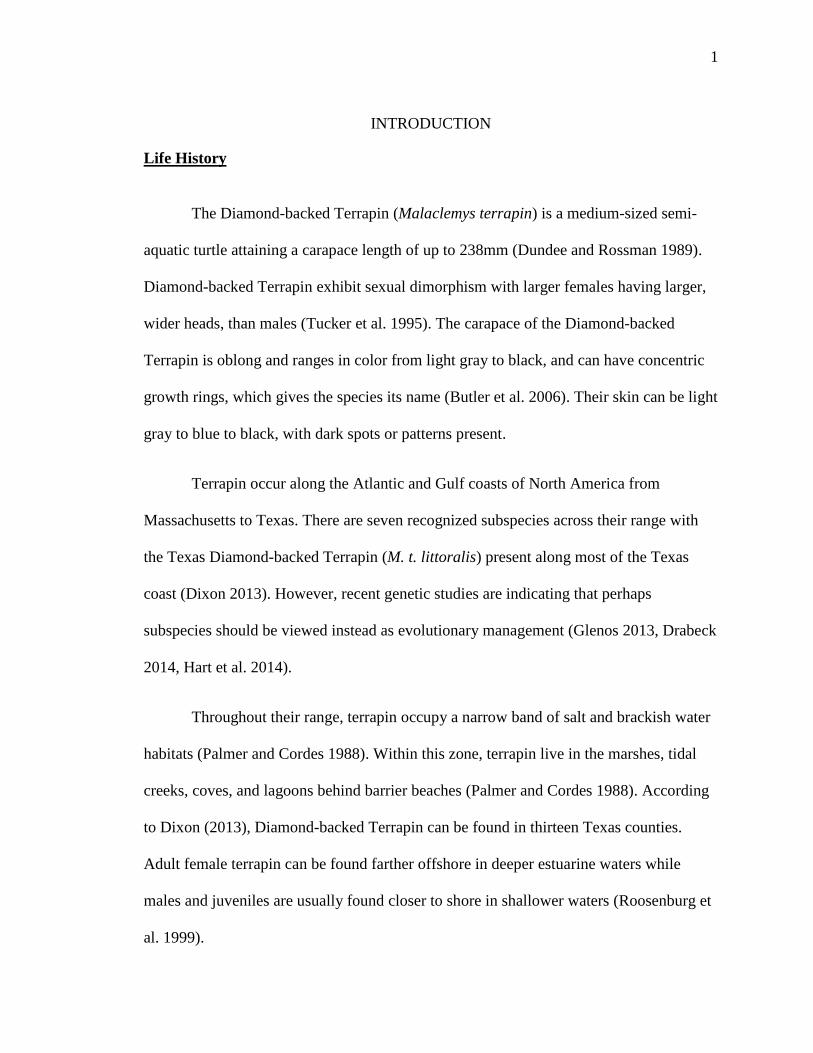
The terrapins were brought to the UHCL animal care facility. They were

maintained individually in plastic tubs containing a small amount (2-3cm) of fresh water

(Figure 9) for up to 48 hours. This is sufficient time for defecation to occur (Tucker et al.

1995). Following this period, the terrapin were released at their capture sites. The

majority of samples were acquired after 48 hour holding times, but due to logistical

constraints some terrapins were only held for 24 hour periods. Also, opportunistic

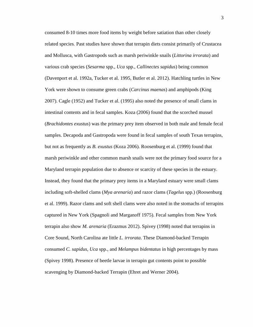
samples were also taken while in the field. Fecal samples were collected from the

containers by carefully draining the water from the tubs. Water from the tubs was poured

over a 0.5mm sieve to collect the fecal matter (Figure 10). The samples were then

recovered and preserved in vials containing 70% ethanol (Figure 11). Some samples were

initially preserved in 10% formalin before changing the solution to ethanol. Using a

0.5mm sieve, the samples were thoroughly rinsed to wash away any preservative before

drying. Samples were dried in a desiccating oven at 100°c for one hour and then weighed

to the nearest tenth of a gram (g) (Figure 12). This process was repeated until sample

weight became stable.

16

Figure 9. Female Diamond-backed Terrapin in storage bin during fecal collection.

Figure 10. Fecal remains on 0.5mm sieve after being poured from collection bin.

17

Figure 11. Two vials containing fecal samples and preservative.

Figure 12. Aluminum container and fecal sample used during drying and weighing.

18

Once reaching a stable weight, the total sample weight was recorded. Each sample

was next separated and sorted into its component parts. Sorting and identification of fecal

remains took place in the lab using forceps and a dissecting microscope. Parts of

organisms found in fecal samples were used to identify to lowest possible taxon. Once a

sample was sorted, each separate taxon was weighed. The proportions of each taxon in an

individual’s sample were then calculated by dividing each taxon weight by the sample

weight. In addition to the previous calculation, a percentage over all samples was

calculated. Weights of each taxon category were summed and divided by the summed

value of all individual sample weights.

Volumetric analysis was also examined and compared with the gravimetric

technique above. Following weighing, the component parts from each sample were

placed into graduated cylinders containing tap water (Figure 13). Displacement for each

taxon was recorded in milliliters (mL) to the nearest 0.1 mL. If a sample displaced less

than 0.1 mL, volume was visually estimated to be either 0.05 or 0.01 mL. The total

sample volume was calculated by adding up the volumes of each taxon group. Size of the

graduated cylinder and water amount in each cylinder used varied depending on size of

the fecal sample being examined. Therefore, large samples were measured in larger

cylinders with more water. Percent volume was calculated in a manner consistent with

the calculations for percent weight described above.

19

Figure 13. Graduated cylinder (25mL) containing partial fecal sample and water.

Fecal sample collection began in April 2013 and concluded May 2014. Terrapins

were only taken from the field for fecal samples when they were found to be active.

Therefore, no terrapins or samples were collected during the months of December or

January when they usually burrow and brumate.

Data Analysis

A technique commonly used for diet analysis studies for terrapin, as well as other

species, is percent frequency of occurrence (Ottonello et al. 2005, Butler 2012 Erazmus

2012). Frequency of occurrence was calculated as the percentage of fecal samples

containing each, individual food item. This is a presence or absence technique.

Percentages of food items by weight and volume were also calculated. These percentages

20

were reached by computing total volume and weight for individual prey items and then

dividing by the total sample (all samples) volume and weight. A modification of this

technique is used for calculating percentages for individual samples. In this case, it is

individual component weight divided by individual sample weight (or volume).

Prior to performing statistical analyses, data were tested for normality (Lengendre

and Lengendre 2012). Datasets did not fit a normal distribution. Therefore, non-

parametric statistical methods were employed for analyses. A Kruskal-Wallis one-way

analysis of variance (KW-ANOVA) was used to analyze differences by sex, season, and

location for both fecal and prey availability data. When an overall significant difference

was found between groups with more than two levels using the overall KW-ANOVA test

Dunn’s multiple comparison test was used post hoc to test for differences between

individual groups (Zar 2009). The Mann-Whitney U-test was used to compare fecal

analysis methods (gravimetric versus volumetric), and it was used to compare air

temperature at ground level to that at breast height. Mann-Whitney testing was used in

those cases because the data was paired. Reported Kruskal-Wallis and Mann-Whitney

values are those that were adjusted for ties when they occurred. For all the below

boxplots, the outer white box represents the interquartile range, inner shaded box is 95%

confidence interval, horizontal line and dot are the median, and whiskers are the data

range, unless otherwise noted. Diversity estimates for diet were calculated using Shannon

Diversity (H’), Evenness (E), and Berger-Parker Index (BPI). Statistical analyses were

performed using Minitab 17 and Microsoft Excel software packages.

21

RESULTS

Prey Availability and Habitat

Over the course of this study, data were collected from a total of 293 prey

quadrats in the field. Data were gathered at both random locations (n = 78) and terrapin

capture locations (n = 215). Terrapins that provided fecal samples made up a subset of

this larger terrapin capture number (n = 55). These data were collected from locations

along the coast of Texas from the following areas: West Bay, East Bay, San Bernard,

Sabine Lake, and Matagorda Bay. West Bay sites made up the vast majority of locations

(n = 276), and consisted of North Deer Island (n = 32), South Deer Island (n = 144),

Sportsman (n = 65), Greens Lake (n = 29), and Sweetwater Lake (n = 6). Multiple prey

quadrats were collected from Texas Point NWR (n = 11) in the Sabine Lake area. East

Bay data were collected from marshes located on Bolivar Peninsula (n = 2). Other

locations with low sample numbers included San Bernard NWR (n = 2) and Matagorda

Bay (n = 2).

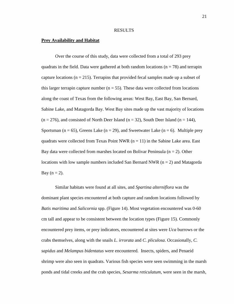
Similar habitats were found at all sites, and Spartina alterniflora was the

dominant plant species encountered at both capture and random locations followed by

Batis maritima and Salicornia spp. (Figure 14). Most vegetation encountered was 0-60

cm tall and appear to be consistent between the location types (Figure 15). Commonly

encountered prey items, or prey indicators, encountered at sites were Uca burrows or the

crabs themselves, along with the snails L. irrorata and C. pliculosa. Occasionally, C.

sapidus and Melampus bidentatus were encountered. Insects, spiders, and Penaeid

shrimp were also seen in quadrats. Various fish species were seen swimming in the marsh

ponds and tidal creeks and the crab species, Sesarma reticulatum, were seen in the marsh,

22

but neither was encountered in quadrats. Prey quadrat data were taken in all seasons

(Table 1). In instances where a terrapin was encountered in a completely aquatic setting,

prey quadrats were not conducted.

Figure 14. Percentage of 1 m2 quadrats with listed species as the dominant plant species at random (n = 78)

and capture (n = 215) locations.

23

Figure 15. Percentage of 1 m2 quadrats with listed vegetation heights at random (n = 78) and capture (n =

215) locations.

Table 1. Number of prey quadrats collected by season.

Season Beginning Date Sample Number

Spring March 20 53

Summer June 21 71

Fall September 22 81

Winter December 21 88

Habitat Quadrats at Random Versus Capture Locations

Multiple significant differences in habitat metrics were detected using Kruskal-

Wallis analysis. The number of plant species present was significantly higher (H = 12.69,

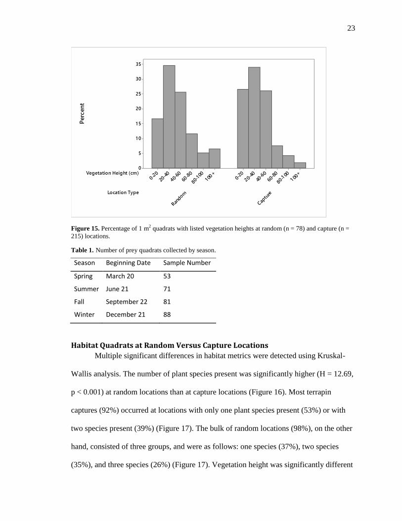
p < 0.001) at random locations than at capture locations (Figure 16). Most terrapin

captures (92%) occurred at locations with only one plant species present (53%) or with

two species present (39%) (Figure 17). The bulk of random locations (98%), on the other

hand, consisted of three groups, and were as follows: one species (37%), two species

(35%), and three species (26%) (Figure 17). Vegetation height was significantly different

24

between random and capture locations (H = 4.48, p = 0.034). Plants at random locations

were significantly taller than at capture locations (Figure 18). Random locations had

significantly higher vegetation cover (H = 8.97, p = 0.003) than did terrapin capture

locations (Figure 19). Significant differences in species coverage were found between

location types as well. Coverage of Batis maritima at random locations was significantly

greater (H = 5.24, p = 0.022) than at terrapin capture locations (Figure 20). Also,

Salicornia spp. coverage was significantly greater (H = 6.47, p = 0.011) at random

locations than at capture locations (Figure 21). No difference (H = 0.80, p = 0.372) was

detected when examining Spartina alterniflora percent cover (Figure 22).

Figure 16. Boxplot depicting location differences of number of plant species in 1 m2 prey quadrats

(Kruskal-Wallis; H = 12.69, p < 0.001). The inner shaded box represents the 95% confidence interval for

the median.

25

Figure 17. Histogram depicting percentage of prey quadrats from random (n = 78) and capture (n = 215)

locations containing a given number of plant species.

Figure 18. Boxplot depicting location differences of vegetation height in 1 m2 prey quadrats (Kruskal-

Wallis; H = 4.48, p = 0.034). The inner shaded box represents the 95% confidence interval for the median.

26

Figure 19. Boxplot depicting location differences of vegetation cover percentage in 1 m2 prey quadrats

(Kruskal-Wallis; H = 8.97, p = 0.003). The inner shaded box represents the 95% confidence interval for the

median.

Figure 20. Boxplot depicting location differences of Batis maritima coverage percentage in 1 m2 prey

quadrats (Kruskal-Wallis; H = 5.24, p = 0.022). The inner shaded box represents the 95% confidence

interval for the median.

27

Figure 21. Boxplot depicting location differences of Salicornia spp. coverage percentage in 1 m2 prey



Figure 22. Boxplot depicting location differences of Spartina alterniflora coverage percentage in 1 m2 prey



28

Habitat Quadrats by Season at Capture Locations

When specifically examining locations where terrapins were captured, no

differences between sexes were found for any of the different habitat categories.

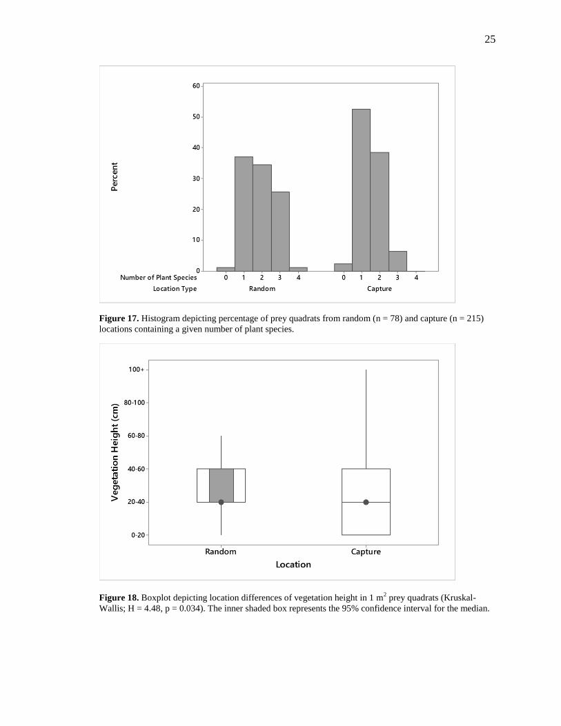
However, significant seasonal differences were detected at capture locations. Seasonal

differences in percent S. alterniflora were found to be strongly significant (H = 31.24, p <

0.001) at capture locations. Diamond-backed Terrapins were encountered in areas with

significantly higher S. alterniflora ground cover in winter and spring than in summer and

fall (Figure 23). No difference between winter and spring was detected. Interestingly, no

significant seasonal differences for total vegetation cover at capture locations were

detected (H = 5.80, p = 0.122). The opposite effect was detected in regards to coverage

by Batis maritima (Figure 24). Capture locations had significantly greater percent cover

of B. maritima in summer and fall than did spring and winter captures (H = 14.61, p =

0.002). Ground cover of Salicornia spp. was significantly higher in fall than in winter and

spring (H = 20.58, p < 0.001). There was no significant difference between fall and

summer (Figure 25).

29

Figure 23. Boxplot depicting seasonal differences of Spartina alterniflora coverage at terrapin capture

locations in 1 m2 prey quadrats (Kruskal-Wallis; H = 31.24, p < 0.001). The inner shaded box represents

the 95% confidence interval for the median. (Significant group differences: a > b)

Figure 24. Boxplot depicting seasonal differences of Batis maritima coverage at terrapin capture locations in 1 m

2 prey quadrats (Kruskal-Wallis; H = 14.61, p = 0.002). The inner shaded box represents the 95%

confidence interval for the median. (Significant group differences: a > b)

WinterSummerSpringFall

70

60

50

40

30

20

1 0

0

Season

% C

over

Bati

s m

ari

tim

a

a a

b b


1 00

80

60

40

20

0

Season

% C

over

Sp

art

ina a

ltern

iflo

ra

a

a

b

b

30

Figure 25. Boxplot depicting seasonal differences of Salicornia spp. coverage at terrapin capture locations in 1 m

2 prey quadrats (Kruskal-Wallis; H = 20.58, p < 0.001). The inner shaded box represents the 95%


Habitat Quadrats by Marsh Site at Capture Locations

Kruskal-Wallis analysis was employed to check for site differences (n = 205).

Most West Bay marshes and Texas Point (n = 10) were included in these analyses. The

West Bay sites examined included South Deer Island (n = 107), North Deer Island (n =

22), Sportsman Road (n = 49), and Greens Lake (n = 17). Due to low sample sizes, San

Bernard (n = 2), Matagorda (n = 2), and Sweetwater (n = 4) sites were excluded from

statistical analysis. Quadrats were not sampled at Bolivar capture locations. Vegetation

height demonstrated significant location differences (H = 10.71, p = 0.030). North Deer

had significantly taller vegetation than Sportsman Road with no other differences

detected between sites (Figure 26). Sites also showed significant differences in number of

plant species found within the quadrats (H = 20.99, p < 0.001). South Deer possessed a

significantly higher number of species than both Sportsman and Texas Point, and a


70

60

50

40

30

20

1 0

0

Season

% C

over

Sali

co

rnia

sp

p.

b b

a

31

significantly higher number of plant species was detected at North Deer compared with

Sportsman (Figure 27).

Figure 26. Boxplot depicting marsh differences at capture locations of vegetation height in 1 m2 prey


interval for the median. (Significant group differences: a > b)

32

Figure 27. Boxplot depicting marsh differences at capture locations of number of plant species in 1 m2

prey quadrats (Kruskal-Wallis; H = 20.99, p < 0.001). The inner shaded box represents the 95% confidence

interval for the median. (Significant group differences: a > b and c > d)

There were no significant differences amongst the West Bay sites when

comparing percent vegetation cover (Figure 28). However, North Deer, South Deer, and

Sportsman had significantly higher vegetative coverage than did Texas Point (H = 14.49,

p = 0.006). When examining percent cover of individuals plant species, there were no

significant site differences in cover of S. alterniflora (H = 6.05, p = 0.196), D. spicata (H

= 9.34, p = 0.053), or Salicornia spp. (H = 8.90, p = 0.064) between locations. Batis

maritima, however, showed significant differences (H = 35.51, p < 0.001) between sites.

South Deer had higher coverage of B. maritima than did North Deer, Sportsman, and

Texas Point (Figure 29). Finally, Spartina patens showed significant location differences

(H = 39.19, p < 0.001). Texas Point quadrats contained higher percentage of S. patens

than did any of the four West Bay sites (Figure 30).

33

Figure 28. Boxplot depicting marsh differences at capture locations of vegetation coverage in 1 m2 prey



Figure 29. Boxplot depicting marsh differences at capture locations of Batis maritima coverage in 1 m2



34

Figure 30. Boxplot depicting marsh differences at capture locations of Spartina patens coverage in 1 m2



Habitat and Temperature

Water and soil temperature data were not statistically analyzed due to low sample

size. However, air temperatures at breast height and ground level were taken more often,

and therefore used in analysis. When analyzing all quadrats with air temperature data,

Mann-Whitney testing detected no significant difference between air temperatures (p =

0.1962) at different heights (Figure 31). Median temperatures (26 °C) at breast height (n

= 276) were no different than temperatures (27 °C) at ground level (n = 195). Therefore,

when further examining temperature relationships below, temperature at ground level

was used since it more accurately reflects to what terrapins are exposed.

35

Figure 31. Boxplot depicting median temperatures at breast height (26.25 °C) and ground level (27. 00 °C)

at both random and capture locations. Significant difference between median values (Mann-Whitney U-

test; p = 0.1962). The inner shaded box represents the 95% confidence interval for the median.

Ground level air temperatures were recorded at a total of 195 locations. A

significant (H = 4.19, p = 0.041) difference in ground level air temperature was detected

between random (n = 61) and capture (n = 134) locations. Median temperatures at capture

locations (27.6 °C) were significantly higher than at random locations (25.3 °C) (Figure

32). At terrapin capture sites, air temperatures exhibited significant differences (H =

23.93, p < 0.001) between vegetation height group classes. The shortest vegetation class

(0-20 cm) exhibited significantly warmer temperatures than three of the taller classes (40-

60 cm, 60-80 cm, 80-100 cm) (Figure 33). The tallest class was not included in analysis

due to few quadrats (n = 4) with that vegetation height. Temperatures were also

significantly different when comparing dominant vegetation (H = 18.57, p < 0.001). Sites

dominated by B. maritima and Salicornia spp. were significantly warmer than S.

alterniflora dominated quadrats (Figure 34). The remaining capture sites (n = 4)

36

dominated by bare ground, D. spicata, and S. patens were again excluded from statistical

analyses due to low sample numbers.

Figure 32. Boxplot depicting location differences of air temperature at ground level recorded at 1 m2 prey



37

Figure 33. Boxplot depicting vegetation height differences in air temperature at ground level recorded at 1

m2 prey quadrats at terrapin capture locations (Kruskal-Wallis; H = 23.93, p < 0.001). The inner shaded box

represents the 95% confidence interval for the median. (Significant group differences: a > b and c > d;

100+ cm height excluded)

Figure 34. Boxplot depicting dominant vegetation differences in air temperature at ground level recorded

at 1 m2 prey quadrats at terrapin capture locations (Kruskal-Wallis; H = 18.57, p < 0.001). The inner shaded

box represents the 95% confidence interval for the median. (Significant group differences: a > b)

38

Prey Quadrats at Random versus Capture Locations

When comparing random locations to terrapin capture locations, there was only

one significant difference in variables detected. Random locations had significantly more

fiddler crab burrows (Kruskal-Wallis; H = 5.57, p = 0.018) than did capture locations

(Figure 35). A significant (H = 0.32, p = 0.571) difference in number of Littorina snails

was also lacking between location types (Figure 36). No differences between locations

were detected when examining average length (H = 1.06, p = 0.302) of L. irrorata or

average width (H = 0.70, p = 0.402). A significant difference in presence C. pliculosa (H

= 3.03, p = 0.082) was also lacking between the location types.

Figure 35. Boxplot depicting fiddler crab (Uca spp.) burrow number differences between random and

terrapin capture locations in 1 m2 prey quadrats (Kruskal-Wallis; H = 5.57, p = 0.018). The inner shaded

box represents the 95% confidence interval for the median.

39

Figure 36. Boxplot depicting Littorina irrorata number differences between random and terrapin capture

locations in 1 m2 prey quadrats (Kruskal-Wallis; H = 0.32, p = 0.571). The inner shaded box represents the

95% confidence interval for the median.

Prey Quadrats by Season at Capture Locations

No significant differences in prey composition were detected between sites where

males were captured versus females in regards to field category of prey item. However,

significant differences were detected in multiple prey conditions by season at terrapin

capture locations. Number of fiddler crab burrows was significantly higher in summer

and winter than in spring and fall (H = 20.99, p < 0.001) (Figure 37). The number of

marsh periwinkle snails counted within prey quadrats also showed significant seasonal

differences (H = 18.58, p < 0.001). Littorina numbers were significantly lower in summer

than in both winter and fall, and spring was also significantly lower than fall (Figure 38).

No seasonal differences in average width (H = 6.60, p = 0.086) or length (H = 6.84, p =

0.077) of L. irrorata were detected.

40

Figure 37. Boxplot depicting seasonal differences of Uca spp. burrows at terrapin capture locations in 1

m2 prey quadrats (Kruskal-Wallis; H = 20.99, p < 0.001). The inner shaded box represents the 95%


Figure 38. Boxplot depicting seasonal differences of Littorina irrorata at terrapin capture locations in 1

m2 prey quadrats (Kruskal-Wallis; H = 18.58, p < 0.001). The inner shaded box represents the 95%

confidence interval for the median. (Significant group differences: a > b and c > d)


1 00

80

60

40

20

0

Season

Nu

mb

er

of

Lit

tori

na

ac a

b

d


40

30

20

1 0

0

Season

Nu

mb

er

of

Fid

dle

r B

urr

ow

s

a a

b b

41

Prey Quadrats by Marsh Site

Analyses to detect prey differences between marshes at terrapin capture locations

in West Bay and Texas Point were conducted using the same number of samples as

previously described for habitat characterization. Significant differences in the number of

fiddler crab burrows were detected between sites (H = 15.48, p = 0.004). South Deer,

North Deer, and Sportsman Road all exhibited significantly higher numbers of burrows

compared to Greens Lake (Figure 39). The numbers of marsh periwinkle snails were

found to be significantly different amongst sites as well (H = 24.12, p < 0.001). Both

North and South Deer had significantly higher counts of Littorina than Sportsman and

Greens Lake marshes (Figure 40). No differences were detected in either average

periwinkle length (H = 0.68, p = 0.953) or width (H = 3.74, p = 0.443). The occurrence of

C. pliculosa was significantly different between sites (H = 15.95, p = 0.003). Horn snails

were encountered in significantly more prey quadrats at South Deer, Sportsman, and

Greens Lake when compared to North Deer, and presence at Sportsman was also

significantly different than Texas Point (Figure 41). Presence of other potential prey

items also showed location differences (H = 17.90, p = 0.001). Other prey items were

encountered at South Deer and Sportsman in significantly more quadrats than at North

Deer (Figure 42).

42

Figure 39. Boxplot depicting marsh differences at capture locations of Uca burrow numbers in 1 m2 prey


interval for the median. (Significant group differences: a > b and c > d)

Figure 40. Boxplot depicting marsh differences at capture locations of Littorina irrorata numbers in 1 m2



43

Figure 41. Marsh differences at capture locations of Cerithidea pliculosa presence in 1 m2 prey quadrats

(Kruskal-Wallis; H = 15.95, p = 0.003). Bars represent each site and show percentage of quadrats where C.

pliculosa was present or absent. (Significant group differences: a > b and c > d)

Figure 42. Marsh differences at capture locations of presence of other potential prey items in 1 m2 prey

quadrats (Kruskal-Wallis; H = 17.90, p = 0.001). Bars represent each site and show percentage of quadrats

where C. pliculosa was present or absent. (Significant group differences: a > b and c > d)

44

Fecal Analysis

A total of 64 fecal samples were collected from terrapin over the course of the

study with 35 female samples and 29 male samples. Samples from terrapins that were

held for approximately 48 hours made up the majority of the collection (n = 45). Fewer

samples came from terrapin that were only held for ~24 hours (n = 8), while the

remainder (n = 11) were collected opportunistically from the field. There were no

significant differences detected between collection methods for either gravimetric

(Kruskal-Wallis; H = 4.91, p = 0.086) or volumetric (Kruskal-Wallis; H = 2.97, p =

0.226) techniques (Figure 43). Therefore, samples collected by all three methods were

analyzed together. Sixty of the samples were collected from different individual terrapins.

However, the four remaining samples represented subsequent samples collected from

individuals that had been sampled previously. These samples were included in the

analyses since they were collected in different seasons or using different techniques (field

sample vs. 48 hour sample). Samples were collected from four West Bay locations:

South Deer Island (n = 35), North Deer Island (n = 8), Sportsman Road (n = 18), and

Greens Lake (n = 2). Also, a single sample of opportunity was taken from a site in the

Matagorda Bay system (n = 1). Samples were collected across all four seasons: spring (n

= 9), summer (n = 25), fall (n = 26), and winter (n = 4) (Table 2).

45

Figure 43. Boxplots depicting total sample volume (mL) (Kruskal-Wallis; H = 2.97, p = 0.226) and weight

(g) (Kruskal-Wallis; H = 4.91, p = 0.086) showing no significant differences in median values between the

three collection techniques. The gray inner box represents the 95% confidence interval for the median.

Table 2. Number of fecal samples collected by season.

Season Beginning Date Sample Number

Spring March 20 9 Summer June 21 25 Fall September 22 26

Winter December 21 4

A total of 22 different items were found in terrapin fecal samples, seven of which

only showed up in one sample. One of these categories, Unknown Crab, was used as a

“catch all” for particles of crab carapace that did not have any identifiable characteristics.

Additionally, some categories were not included in most analyses due to rarity, being

abiotic in nature, or if unidentifiable biological matter. The majority of abiotic items

encountered were sediments, which included small rocks, sand, or shell hash. An item

that appeared to be a small amount of plastic was found in a single sample. Most

46

terrapins were found to have consumed more than one, biotic item (mode = 3), and the

number of different items found in an individual sample ranged from 1-8 items (Figure

44). Prey items were found from the following animal groups: Gastropoda, Decapoda,

Bivalvia, Insecta, Araneae, and Actinopterygii. There was one instance where an

unknown egg cluster was found in a sample. Vascular plants and algae were also

commonly found in samples. Plant material consisted of the marsh species S. alterniflora

and Salicornia spp, and all materials (stems, leaves, seeds, etc.) were grouped together.

Figure 44. Frequency of varying numbers of prey items found in individual fecal samples (n = 64).

Diversity Indices

Estimates of dietary diversity varied by fecal analysis technique (Table 3). Overall

Shannon-Weiner (H’) diversity indices for terrapin diet were slightly higher for

volumetric analysis (H’mL = 1.34) than for gravimetric analysis (H’g = 1.13). Overall

Shannon Evenness (E) were again higher for volumetric (EmL = 0.46) than for gravimetric

(Eg = 0.39). Berger-Parker Index (BPI) values were similar between both techniques

47

(BPIg = 0.48, BPImL = 0.49). The diets of male terrapins (H’g = 1.41, H’mL = 1.56) were

shown to be more diverse than that of females (H’g = 0.99, H’mL = 1.18) using either fecal

analysis technique. Male diets also exhibited a higher evenness (E) than females. Based

on the results of gravimetric analysis, male diets had an Eg of 0.52 compared to the diet

of females at 0.37. Volumetric analysis yielded similar evenness results for males (EmL =

0.58) and females (EmL = 0.43). Berger-Parker Index scores were similar across all

categories and techniques. Volumetric BPI for male terrapins (0.46) was slightly lower

than BPI for females (0.50). Whereas, male gravimetric BPI scores (0.52) were higher

than females (0.47).

Table 3. Shannon-Weiner (H'), Shannon Evenness (E), and Berger-Parker (BPI) indices of diversity for M.

t. littoralis diet. Estimates are given for total samples, males, and females for both gravimetric and

volumetric techniques.

Gravimetric (g) Volumetric (mL)

Total Male Female

Total Male Female

Shannon-Weiner (H') 1.13 1.41 0.99

1.34 1.56 1.18

Shannon Evenness (E) 0.39 0.52 0.37

0.46 0.58 0.43

Berger-Parker (BPI) 0.48 0.52 0.47 0.49 0.46 0.50

Frequency of Occurrence

During the study, Diamond-backed Terrapins most frequently ingested

Gastropods (Table 4). Gastropods, composed of three identified species, were found in

70% of fecal samples. The percent occurrence of Gastropods was lower in males (62%)

in contrast to females (77%). The most frequently encountered Gastropod was the plicate

horn snail (Cerithidea pliculosa) (59%) followed by marsh periwinkle snails (Littorina

irrorata) (25%). There was little difference in the occurrence of C. pliculosa between

males (58%) and females (60%). L. irrorata occurred in 43% of female samples, but only

3% of male samples. The third Gastropod species found in terrapin diet was eastern

48

melampus (Melampus bidentatus). Melampus snails were found in 8% of all samples,

10% of male samples and 6% of female samples.

Table 4. Frequency of occurrence of prey items found in terrapin fecal samples. Percentages given for

total, male, and female samples.

% Frequency of Occurrence

Total Male Female

Prey Item (n = 64) (n = 29) (n = 35)

Class Gastropoda

70.3 62.1 77.1

Cerithidea pliculosa Plicate Horn Snail 59.4 58.6 60.0

Littorina irrorata Marsh Periwinkle 25.0 3.4 42.9

Melampus bidentatus Eastern Melampus 7.8 10.3 5.7

Class Bivalvia

9.4 6.9 11.4

Mulina lateralis Dwarf Surf Clam 6.3 3.4 8.6

Solen viridis Green Jackknife Clam 1.6 0.0 2.9

Arcidae A Ark Clam A 1.6 0.0 2.9

Arcidae B Ark Clam B 1.6 3.4 0.0

Subphylum Crustacea

Order Decapoda

67.2 79.3 57.1

Uca spp. Fiddler Crabs 40.6 41.4 40.0

Callinectes sapidus Blue Crab 21.9 31.0 14.3

Sesarma reticulatum Purple Marsh Crab 3.1 6.9 0.0

Unknown Crab

15.6 13.8 17.1

Unknown Shrimp

1.6 3.4 0.0

Order Sessilia

Balanus sp. Barnacle 1.6 0.0 2.9

Class Insecta

18.8 13.8 22.9

Order Araneae

7.8 10.3 5.7

Class Actinopterygii

14.1 17.2 11.4

Kingdom Plantae

78.1 82.8 71.4

Algae (Monran and/or

Protista)

4.7 0.0 8.6

Unknown Egg Cluster 1.6 3.4 0.0

49

The second most common animal group was Decapod crustaceans (Table 4).

Decapods were categorized into five groups, and were found in 67% of all samples. A

higher percentage of male samples (79%) contained Decapoda compared to female

samples (57%). Fiddler crabs (Uca spp.) were found in 41% of all samples and did not

differ much between males (41%) and females (40%). Blue crab (Callinectes sapidus)

remains were found in 22% of terrapin samples. There were differences in blue crab

occurrence between males (31%) and females (14%). Purple marsh crabs (Sesarma

reticulatum) were not encountered in any female samples; however, 7% of male samples

contained this species. This accounts for only 3% of total samples. Unidentifiable

particles of crab carapace found in samples were put into the category Unknown Crab.

Items in this category were found in 16% of all samples, and within 14% of male samples

and 17% of female samples. An unidentified shrimp was found in a single male sample

(3%), which is less than 2% of the total. However, the shrimp was largely intact and

hardly digested which may indicate contamination of the sample in some way rather than

ingestion by the turtle.

The most frequently encountered group, overall, was vascular plants (Table 4).

Plant material of some sort showed up in 78% of all samples, and was more frequently

observed in male (83%) versus female (71%) samples. Infrequently consumed items

included algae, Bivalvia, Araneae (spiders), Insecta, and Actinopterygii (ray-finned

fishes). Bivalves consisted of four different types; two were identified to species while

the other two could only be identified to family. The species identified were dwarf surf

clam (Mulina lateralis) and green jackknife clam (Solen viridis), while the two others

appear to be from the family Arcidae (ark clams). Three families of spiders were

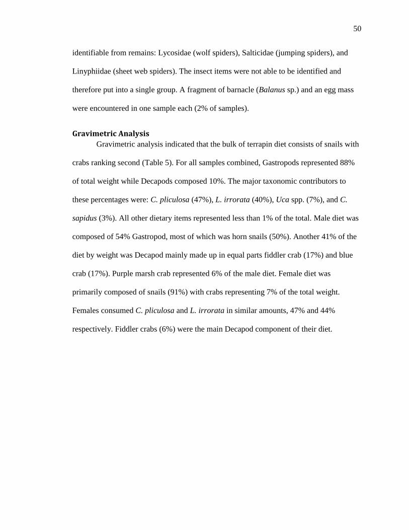
50

identifiable from remains: Lycosidae (wolf spiders), Salticidae (jumping spiders), and

Linyphiidae (sheet web spiders). The insect items were not able to be identified and

therefore put into a single group. A fragment of barnacle (Balanus sp.) and an egg mass

were encountered in one sample each (2% of samples).

Gravimetric Analysis

Gravimetric analysis indicated that the bulk of terrapin diet consists of snails with

crabs ranking second (Table 5). For all samples combined, Gastropods represented 88%

of total weight while Decapods composed 10%. The major taxonomic contributors to

these percentages were: C. pliculosa (47%), L. irrorata (40%), Uca spp. (7%), and C.

sapidus (3%). All other dietary items represented less than 1% of the total. Male diet was

composed of 54% Gastropod, most of which was horn snails (50%). Another 41% of the

diet by weight was Decapod mainly made up in equal parts fiddler crab (17%) and blue

crab (17%). Purple marsh crab represented 6% of the male diet. Female diet was

primarily composed of snails (91%) with crabs representing 7% of the total weight.

Females consumed C. pliculosa and L. irrorata in similar amounts, 47% and 44%

respectively. Fiddler crabs (6%) were the main Decapod component of their diet.

51

Table 5. Percentages of prey items by weight (g) found in terrapin fecal samples. Percentages given for


% by Weight (g)

Total Male Female

Prey Item (n = 64) (n = 29) (n = 35)

Class Gastropoda

87.6 54.5 91.3




Class Bivalvia

0.08 0.02 0.08





Subphylum Crustacea

Order Decapoda

10.4 40.6 6.9




Unknown Crab

0.3 0.9 0.2

Unknown Shrimp

0.0009 0.009 0.0

Order Sessilia


Class Insecta

0.007 0.03 0.005

Order Araneae

0.004 0.02 0.002


0.2 1.6 0.05

Kingdom Plantae

0.4 1.0 0.3

Algae (Moneran and/or

Protista)

0.2 0.0 0.4


Based on the results of Kruskal-Wallis ANOVA multiple significant differences

in percent weight between the diets of male and female terrapins were detected. Females

52

consumed significantly more periwinkle snails (H = 13.28, p < 0.001) and total

Gastropods (H = 5.95, p = 0.015) than did males (Figure 45 and Figure 46). In contrast,

males showed a significantly higher percentage of blue crab consumption (H = 3.87, p =

0.049) and Decapods overall (H = 5.30, p = 0.021) than females (Figure 47 and Figure

48). Finally, male terrapin exhibited significantly higher percentage intake of plant matter

(H = 6.02, p = 0.014) in comparison to females (Figure 49). No other significant (p ≤

0.05) differences in quantities or percentages of dietary items were detected between the

sexes.

Figure 45. Boxplot depicting percent weight differences between male (M) and female (F) diet of Littorina

irrorata (Kruskal-Wallis; H = 13.28, p < 0.001). The inner shaded box represents the 95% confidence


53

Figure 46. Boxplot depicting percent weight differences between male (M) and female (F) diet of Total

Gastropoda (Kruskal-Wallis; H = 5.95, p = 0.015). The inner shaded box represents the 95% confidence


Figure 47. Boxplot depicting percent weight differences between male (M) and female (F) diet of

Callinectes sapidus (Kruskal-Wallis; H = 3.87, p = 0.049). The inner shaded box represents the 95%

confidence interval for the median.

54

Figure 48. Boxplot depicting percent weight differences between male (M) and female (F) diet of Total

Decapoda (Kruskal-Wallis; H = 5.30, p = 0.021). The inner shaded box represents the 95% confidence


Figure 49. Boxplot depicting percent weight differences between male (M) and female (F) diet of Plantae


median.

55

Due to winter having a small sample size (n = 4), seasonal statistical analyses

were limited to spring, summer, and fall. However, winter data were included in

graphical representations. Significant seasonal variations in diet were evaluated using

Kruskal-Wallis analysis and the post hoc Dunn’s multiple range test. A significant

seasonal difference was found in the percent weight of total Gastropods (H = 10.54, p =

0.005). Consumption of snails was significantly higher during spring and fall compared

with summer (Figure 50). Highly significant (H = 15.98, p < 0.001) seasonal differences

were detected in the percent of diet composed of fiddler crabs. Terrapins consumed a

higher percentage of fiddler crabs in summer in comparison to other seasons (Figure 51).

Consumption of blue crabs also varied seasonally (H = 8.15, p = 0.017). Diamond-backed

Terrapin consumed a significantly higher percentage of blue crab in the fall than in

summer (Figure 52). Seasonal differences in consumption of total Decapoda approached

statistical significance (H = 5.79, p = 0.055) (Figure 53). Diamond-backed Terrapin

consumed a significantly higher percentage of spiders (H = 7.00, p = 0.03) in fall than in

summer (Figure 54). Based on results of the Kruskal-Wallis test (H = 11.74, p = 0.003)

seasonal differences in the amount of plant matter ingested by terrapin were detected. The

amount of plant material in their diet was significantly higher in fall and summer than in

spring (Figure 55).

56

Figure 50. Boxplot depicting seasonal dietary differences in percent weight of total Gastropoda (Kruskal-


(Significant group differences: a > b; winter excluded from analysis)

Figure 51. Boxplot depicting seasonal dietary differences in percent weight of Uca spp. (Kruskal-Wallis; H

= 15.98, p < 0.001). The inner shaded box represents the 95% confidence interval for the median.



1 00

80

60

40

20

0

Season

Uca s

pp

. (g

) %

a

b b


1 00

80

60

40

20

0

Season

To

tal

Gast

rop

od

a (

g)

%

a a b

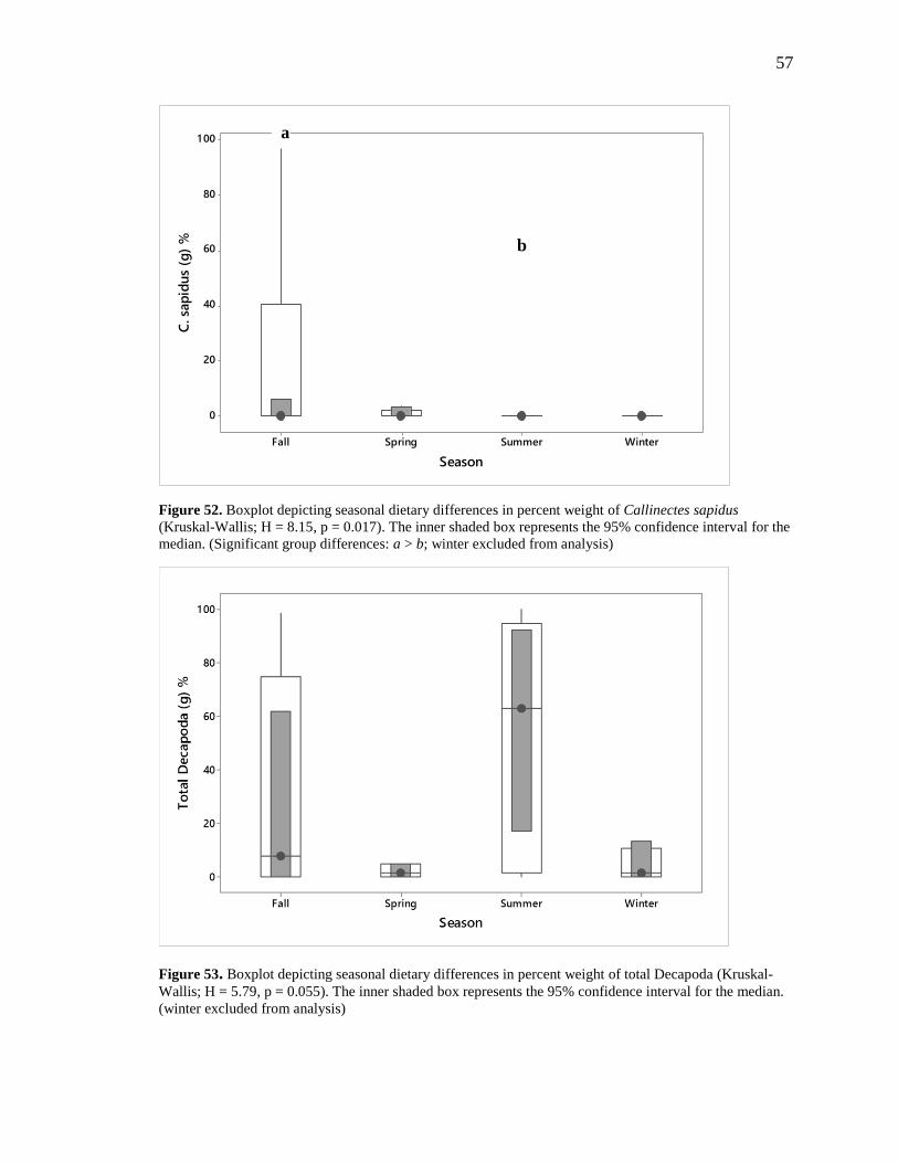
57

Figure 52. Boxplot depicting seasonal dietary differences in percent weight of Callinectes sapidus


median. (Significant group differences: a > b; winter excluded from analysis)

Figure 53. Boxplot depicting seasonal dietary differences in percent weight of total Decapoda (Kruskal-


(winter excluded from analysis)


1 00

80

60

40

20

0

Season

C. sa

pid

us

(g)

%

a

b

58

Figure 54. Boxplot depicting seasonal dietary differences in percent weight of Araneae (Kruskal-Wallis; H

= 7.00, p = 0.03). The inner shaded box represents the 95% confidence interval for the median. (Significant

group differences: a > b; winter excluded from analysis)

Figure 55. Boxplot depicting seasonal dietary differences in percent weight of vascular plants (Kruskal-




60

50

40

30

20

1 0

0

Season

Pla

nta

e (

g)

%

a a b


0.50

0.25

0.00

-0.25

-0.50

Season

Ara

nea (

g)

%

b a

59

In order to examine dietary differences between sites, results of gravimetric

analyses from terrapin captured at three West Bay sites including South Deer (n = 35),

Sportsman Road (n = 18), and North Deer (n = 8) were included in the formal statistical

analyses. Greens Lake (n = 2) and Matagorda (n = 1) were not included in the formal data

analysis due to low sample size. While not statistically analyzed, Greens Lake terrapin

diets were dominated by > 99% C. pliculosa. The Matagorda diet sample contained M.

bidentatus (73%) and Uca spp. (27%).

A significant difference in percent horn snails found in terrapin diet was detected

between the three sites (H = 6.60, p = 0.037). Both North Deer and Sportsman Road

terrapins had significantly higher percentages of C. pliculosa in their fecal samples than

South Deer samples (Figure 56). Significant location differences in Uca spp.

consumption (H = 6.43, p = 0.04) were also detected. Terrapin from Sportsman Road

were found to have significantly greater percentages of fiddler crabs in their diets than

both those from North and South Deer (Figure 57).

60

Figure 56. Boxplot depicting dietary differences by location in percent weight of Cerithidea pliculosa


median. (Significant group differences: a > b)

Figure 57. Boxplot depicting dietary differences by location in percent weight of Uca spp. (Kruskal-


(Significant group differences: a > b)

61

Volumetric Analysis

Gastropods made up the highest percentage (79%) of total terrapin diet by percent

volume (Table 6). Decapods made up the second highest percentage (15%) of total diet.

Plant material represented 3% of the total terrapin diet. All other items contributed less

than 1% of the total volume. Plicate horn snails were the largest contributor (48%) to the

Gastropod category followed by marsh periwinkles (30%). Overall the main Decapod

species consumed by volume were Uca spp. (10%) and C. sapidus (3%). Male terrapin

consumed 47% snails by volume, which were composed of 45% C. pliculosa. Crab

species represented 39% of the diet of male terrapins. Fiddler crabs (19%) and blue crabs

(14%) were the dominant Decapod taxa consumed. Another Decapod species, Sesarma

reticulatum, represented the reaming 5% consumed. Plants made up a fairly large portion

(8%) of the male terrapin diet. The female terrapin diet consisted of Gastropoda at 84%

by volume, 49% horn snails and 35% marsh periwinkle. In contrast to males, Decapods

made up less of female diet (10%). Fiddler crabs represented 9% of the Decapod volume,

while blue crab contributed only 1%. Plant material composed 2% of the female terrapin

diet.

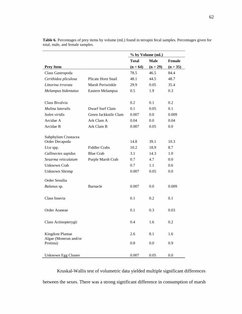
62

Table 6. Percentages of prey items by volume (mL) found in terrapin fecal samples. Percentages given for


% by Volume (mL)

Total Male Female

Prey Item (n = 64) (n = 29) (n = 35)

Class Gastropoda

78.5 46.5 84.4




Class Bivalvia

0.2 0.1 0.2





Subphylum Crustacea

Order Decapoda

14.8 39.1 10.3




Unknown Crab

0.7 1.1 0.6

Unknown Shrimp

0.007 0.05 0.0

Order Sessilia


Class Insecta

0.1 0.2 0.1

Order Araneae

0.1 0.3 0.03


0.4 1.6 0.2

Kingdom Plantae

2.6 8.1 1.6

Algae (Moneran and/or

Protista)

0.8 0.0 0.9


Kruskal-Wallis test of volumetric data yielded multiple significant differences

between the sexes. There was a strong significant difference in consumption of marsh

63

periwinkle snails between the sexes (H = 13.28, p < 0.001), with females consuming

more than males (Figure 58). Females also consumed significantly more Gastropods (H =

6.25, p = 0.012) than did males (Figure 59). Male terrapins were found to have

significantly higher percentages of C. sapidus (H = 4.02, p = 0.045) in their diet than

females (Figure 60). Total Decapoda intake was significantly greater in males (H = 4.15,

p = 0.042) than females (Figure 61). Finally, male fecal samples contained higher

percentages of plant material (H = 9.97, p = 0.002) than what was found in female fecal

samples (Figure 62).

Figure 58. Boxplot depicting percent volume differences between male (M) and female (F) diet of

Littorina irrorata (Kruskal-Wallis; H = 13.28, p < 0.001). The inner shaded box represents the 95%


64

Figure 59. Boxplot depicting percent volume differences between male (M) and female (F) diet of Total

Gastropoda (Kruskal-Wallis; H = 6.25, p = 0.012). The inner shaded box represents the 95% confidence


Figure 60. Boxplot depicting percent volume differences between male (M) and female (F) diet of

Callinectes sapidus (Kruskal-Wallis; H = 4.02, p = 0.045). The inner shaded box represents the 95%


65

Figure 61. Boxplot depicting percent volume differences between male (M) and female (F) diet of Total

Decapoda (Kruskal-Wallis; H = 4.15, p = 0.042). The inner shaded box represents the 95% confidence


Figure 62. Boxplot depicting percent volume differences between male (M) and female (F) diet of Plantae


median.

66

Seasonal variations in volumetric diet data were detected using Kruskal-Wallis

ANOVA. There was a significant seasonal difference (H = 10.69, p = 0.005) in total

Gastropoda consumed. Based on results of Dunn’s multiple comparison test terrapin

captured during the spring and fall had significantly higher amounts of total Gastropods

in comparison to summer (Figure 63). A significant seasonal difference for Uca spp. was

detected as well (H = 16.33, p < 0.001). Terrapin consumed higher percentages of fiddler

crab species in summer compared to both fall and spring (Figure 64). There was a

significant seasonal difference for C. sapidus (H = 8.26, p = 0.016). Fall was significantly

higher than summer in percentage of blue crabs consumed (Figure 65). There was also a

significant seasonal difference in total Decapoda (H = 7.23, p = 0.027) consumption. The

consumption of Decapods was significantly higher in the summer in comparison to spring

(Figure 66). Significant seasonal differences in consumption of spiders were detected (H

= 7.00, p = 0.030). A higher percentage of spiders were consumed in fall than in summer

(Figure 67). Terrapin captured during the summer and fall ingested a significantly higher

(H = 14.44, p = 0.001) percentage of plant material in comparison to spring specimens.

Fall was also significantly different than summer (Figure 68).

67

Figure 63. Boxplot depicting seasonal dietary differences in percent volume of total Gastropoda (Kruskal-



Figure 64. Boxplot depicting seasonal dietary differences in percent volume of Uca spp. (Kruskal-Wallis;

H = 16.33, p < 0.001). The inner shaded box represents the 95% confidence interval for the median.



1 00

80

60

40

20

0

Season

Uca s

pp

. (m

L)

%

a

b b


1 00

80

60

40

20

0

Season

To

tal

Gast

rop

od

a (

mL)

%

a a b

68

Figure 65. Boxplot depicting seasonal dietary differences in percent volume of Callinectes sapidus


median. (Significant group differences: a > b; winter excluded from analysis)

Figure 66. Boxplot depicting seasonal dietary differences in percent volume of total Decapoda (H =

7.23, p = 0.027). The inner shaded box represents the 95% confidence interval for the median. (Significant

group differences: a > b; winter excluded from analysis)


1 00

80

60

40

20

0

Season

To

tal

Decap

od

a (

mL)

%

a

b


90

80

70

60

50

40

30

20

1 0

0

Season

C. sa

pid

us

(mL)

%

a

b

69

Figure 67. Boxplot depicting seasonal dietary differences in percent volume of Araneae (H = 7.23, p =

0.027). The shaded box represents the data range. (Significant group differences: a > b; winter excluded

from analysis)

Figure 68. Boxplot depicting seasonal dietary differences in percent volume of vascular plants (Kruskal-


(Significant group differences: a > b and c > d; winter excluded from analysis)


40

30

20

1 0

0

Season

Pla

nta

e(m

L)

%

a c

a d

dD

d d

b

a b


6

5

4

3

2

1

0

Season

Ara

nea (

mL)

%

70

During examination of dietary differences between sites, results of volumetric

analyses from terrapin captured at three West Bay sites including South Deer (n = 35),

Sportsman (n = 18), and North Deer (n = 8) were included in the formal statistical

analyses. Greens Lake (n = 2) and Matagorda (n = 1) were not included in the formal data

analysis due to low sample size. The Matagorda sample consisted of M. bidentatus (65%)

and Uca spp. (32%). Greens Lake samples were almost entirely composed of C. pliculosa

(> 99%). Based on volumetric data a significant difference in percent horn snails found in

terrapin diet was detected between the sites (H = 6.91, p = 0.032). Terrapin collected at

Sportsman Road were found to have significantly higher percentages of C. pliculosa in

their fecal samples than South Deer samples (Figure 69). Significant location differences

in the percent of diet composed of Uca spp. (H = 6.11, p = 0.047) were also detected.

Terrapin from the Sportsman Road area had significantly greater percentages of fiddler

crabs in their diets than both those from North and South Deer (Figure 70).

71

Figure 69. Boxplot depicting dietary differences by location in percent volume of Cerithidea pliculosa


median. (Significant group differences: a > b)

Figure 70. Boxplot depicting dietary differences by location in percent volume of Uca spp. (Kruskal-


(Significant group differences: a > b)

72

Volumetric vs. Gravimetric

No significant differences were found between most prey groups when comparing

percent volume (n = 64) versus percent weight (n = 64) using Mann-Whitney U-test.

There was, however, one group with a significant difference. Percentage of plant matter

was found to yield significant differences between the two analysis techniques (p =

0.0204). The median value for percentages of plant material based on volumetric analysis

(1.613) was significantly higher than gravimetric analysis (0.243) (Figure 71). While

there are no other significant differences, volumetric analyses did result in slightly higher

dietary percentages for a number of other groups especially crabs when compared to

gravimetric (Table 5 and Table 6).

Figure 71. Boxplot depicting median values for gravimetric (0.243) and volumetric (1.613) for Plantae

percentage in terrapin diet. Significant difference between median values (Mann-Whitney U-test; p =

0.0204). The white box represents the interquartile range, colored box is 95% confidence interval,

horizontal line and dot are the median, and whiskers are the data range.

73

DISCUSSION

Effects of Habitat on Terrapin Distribution

Saltmarsh habitats throughout this study were found to have similar vegetation

structures. Marsh vegetation tended to be less than a meter tall (≤60 cm), and composed

of three common species. The dominant plant species encountered over the course of this

study was smooth cordgrass (Spartina alterniflora). It was present in over half of the prey

quadrats including both random survey and capture locations. Two less dominant but

frequently encountered plants included Batis maritima and Salicornia spp. Terrapins

were found significantly more often in areas of the marsh with low plant species richness

(one or two species) compared to random locations. Overall percent vegetation cover

within a quadrat was significantly higher at random locations than at points of capture.

Vegetation was also significantly taller at random locations. These results suggest

terrapins prefer areas without an extremely complex plant structure. Dense vegetation

likely impedes efficient locomotion by terrapins. However, it is also possible that

terrapins utilize areas with vegetation coverage similar to those detected within random

quadrats, but may have gone undetected in such areas. Observers could have difficulty

locating terrapins in areas of dense or tall vegetation.

No significant difference in S. alterniflora density was detected between capture

and random locations. However, the other common species showed differences. Not

finding differences in coverage of S. alterniflora gives credence to its commonality

across Texas saltmarshes. Coverage of both B. maritima and Salicornia were

significantly higher at random locations. These species are usually found at slightly

higher marsh elevations than smooth cordgrass. These results may indicate infrequent

74

usage of areas with high coverage of these species by terrapins. The random sampling

method likely resulted in collection of data in some quadrats located at higher elevations

where terrapin are infrequently observed.

Significant differences in seasonal vegetation density preference or any other

habitat metrics were not detected between male and female terrapins. However, Clarkson

(2012) found that male terrapins on South Deer Island occurred more frequently in less

dense vegetation during March but in denser vegetation during August. In contrast, South

Deer Island females occurred in denser vegetation during February, May, and August in

contrast to the months of March and April (Clarkson 2012). Those findings differ from

the results of this study where no sexual differences in use of vegetation density were

detected. This study did, however, document overall seasonal changes in habitat use by

terrapin.

During winter and spring, terrapins were more often captured in areas containing

higher coverage of S. alterniflora. While in the summer and fall, terrapins were captured

in areas consisting of higher density B. maritima. These seasonal habitat differences may

be attributable in part to differing tidal amplitudes observed during each season.

Terrapins in fall were also caught in areas of higher Salicornia cover. Tidal waters more

often inundate areas containing Batis and Salicornia at high tides in summer and fall due

to prevailing south winds. Diamond-backed Terrapin are known to follow tides as they

rise into the marsh (Tucker 1995). It is also possible thermoregulation is a factor in

habitat preference. Temperature results from this study indicate that ground level air

temperatures of S. alterniflora dominated quadrats were significantly cooler than those of

B. maritima and Salicornia. Therefore, it is unlikely that terrapin are using smooth

75

cordgrass for warmth in winter. Past studies indicate that differences in plant canopy

structure can affect microclimate resulting in lower maximum soil temperature and lower

daily temperature amplitudes (Teasdale and Mohler 1993). The general structure of S.

alterniflora, which is usually taller and denser than Batis and Salicornia, could result in

more stable temperatures and less variation in temperature over short and long time

periods. Whereas, the shorter, more open canopy structure of both Batis and Salicornia

allows for more sunlight to reach the marsh surface and likely provides less insulation

allowing for greater temperature swings. According to Akins et al. (2014), terrapins can

experience drastic temperature changes depending on season and time of day. In North

Carolina saltmarshes, terrapins experiences daily temperature variations of 7 °C in

summer and 9 °C in winter (Williard and Harden 2011). Cordgrass structure also may

make it more suitable for predator avoidance for the same reasons. Thus, S. alterniflora

likely makes for good burrowing habitat during cold weather brumation.

Significant differences in habitat structure between marshes were detected based

on data from capture location solely. These comparisons were made between capture

locations at the three West Bay sites (North Deer, South Deer, Sportsman, and Greens

Lake) and Texas Point. The only significant difference in vegetation height detected was

between North Deer and Sportsman Road. The difference in vegetation height between

North Deer and Sportsman Road may be due to different species composition between

the two marshes. North Deer’s taller vegetation when compared to Sportsman Road could

be due to the presence of larger expanses of the taller S. alterniflora or less B. maritima

or Salicornia. The amount of Batis cover was however low at both North Deer and

Sportsman Road. The Sportsman Road and Texas Point marshes had a lower number of

76

plant species present in quadrats than those of South Deer Island. The number of species

was also significantly lower at Sportsman Road when compared to North Deer. Based on

these results, South Deer Island’s wetlands have more complex habitat than both

Sportsman Road and Texas Point, and North Deer exhibited higher complexity than

Sportsman. These differences in habitat complexity could potentially affect types and

numbers of prey species (Tews et al. 2004).

West Bay marshes all had similar vegetation coverage, and all but Greens Lake

were significantly greater than Texas Point. However, this may simply be a product of

bias due to the locations where most of the Texas Point data were collected. The Texas

Point captures were few in number and made in areas of little vegetation. In contrast all

the West Bay sites showed similar vegetation coverage due to proximity of all the sites.

However, there were differences in species coverage in West Bay. Coverage of Batis at

South Deer was higher than Texas Point, North Deer Island, and Sportsman Road.

While South Deer had no significant height differences compared to other marsh

sites, the island’s higher coverage of B. maritima contributes to a somewhat lower

vegetation height. Marshes at Texas Point had higher composition of S. patens than did

all other sites. In fact, terrapin were never captured in association with saltmeadow

cordgrass in West Bay. This species occurs infrequently at the West Bay sites (personal

observation). The presence of saltmeadow cordgrass at Texas Point suggests that the area

has slightly higher elevations and/or lower salinities based on the environmental

preferences of this species (Bertness 1991).

77

Effects of Prey Availability on Terrapin Distribution

Terrapin capture locations and random locations showed similar numbers of L.

irrorata and C. pliculosa suggesting uniform distribution and availability of these snails

found within quadrats throughout the studied marshes. On the other hand, higher numbers

of Uca burrows were observed at randomly surveyed quadrats. Fecal results demonstrate

that terrapin take fiddler crabs in large numbers, specifically in summer. The fact that

random sites had higher burrow counts than capture locations, with no other detected

differences, suggests prey availability is not a driving factor in terrapin distribution

within Texas saltmarshes. These findings are similar to previous terrapin prey studies

(Tucker et al. 1995, Whitelaw and Zajac 2002).

As previously stated there were no significant differences in prey availability

metrics between male and female capture locations. Marsh periwinkle snail numbers

were highest in fall and winter, and lowest in summer. Fall numbers were also

significantly higher than spring counts. Tidal amplitude could explain the high fall

numbers, as the tides are still high which drives the snails further up plant stems making

for more obvious targets to count. The same effect should also be seen in summer which

makes the low Littorina numbers during that time period difficult to explain. However,

terrapins may be showing a preference for areas containing abundant fiddler crabs in

summer rather than areas with high counts of periwinkle snails. Fecal samples support

this claim that areas with Uca spp. being visited more often in summer months than areas

containing high amounts of L. irrorata.

78

The only other observed seasonal prey differences were in numbers of fiddler crab

burrows. Fiddler burrow counts were highest during the summer and winter seasons. I

observed higher Uca spp. activity in the summer months, which is discussed in detail

later. Two species of fiddler crab were collected during this time of high activity at South

Deer Island, Uca rapax and U. panacea. This is supported by and explains the higher

burrow numbers counted during this season. Summer months generally had higher tidal

amplitudes than winter, and high tides make it difficult to detect burrows. The opposite

tidal effect is likely responsible for the winter burrow numbers. Low winter tides expose

the marsh surface making counts easier to perform. Therefore, the higher counts in the

summer were likely due to higher numbers of living fiddler crabs while the high numbers

in winter months were likely due to the higher probability of detection of older but still

existent burrows from the earlier summer and fall periods. Data from a Louisiana study

showed increased Uca spinicarpa burrow densities in the summer within lower reaches

of the marsh (Mouton, Jr. and Felder 1996). That study also noted high burrow densities

in the early fall (September) for U. longisignalis (Mouton, Jr. and Felder 1996).

As with other analyses, individual marshes displayed differences in prey

availability. Surprisingly, many of these differences were found between West Bay marsh

sites. The only detected difference for Texas Point was in presence of horn snails, as none

were encountered in Texas Point quadrats. For every species exhibiting a significant

difference in numbers, South Deer Island quadrats consistently displayed higher numbers

in comparison to other locations. As previously suggested, the more complex habitat

found at South Deer likely explains the abundance of different prey items found there

(Tews et al. 2004). The numbers and types of available prey at Sportsman Road marsh

79

were similar to South Deer with only one significant difference between the two. Both

South and North Deer Islands exhibited higher numbers of Littorina snails than the

nearby, barrier island and mainland sites at Sportsman and Greens Lake.

Greens Lake stands out from the other sites, specifically the other West Bay

marshes, as having basically no fiddler burrows counted within capture quadrats. Greens

Lake also had significantly lower numbers of periwinkle snails compared to the Deer

Islands. Large percentages of capture locations at Greens Lake contained C. pliculosa.

The difference in prey availability at Greens Lake likely explains why the two fecal

samples from Greens were almost exclusively composed of horn snails.

These results lead to somewhat contradictory conclusions. Differences in multiple

prey metrics were not detected over large geographic distances (Texas Point to West

Bay), but were observed between areas that are much closer together (multiple

differences in West Bay). This may simply reflect an artifact of sample size. Increased

effort at Texas Point may be able to identify differences in prey abundance at this site in

comparison to the West Bay Sites.

Terrapin Diet Analyses

Terrapins on the Upper Texas Coast consumed multiple prey species. Contrary to

previous studies (Tucker et al. 1995), male Texas Diamond-backed Terrapin displayed

higher diversity in their diets than females. However, the diversity of prey items was

found to be lower in Texas than in the South Carolina study. The two most important

groups of prey items in the diet of Texas Diamond-backed Terrapin on the Upper Coast

found in this study are Decapoda and Gastropoda. Prey items from these groups were

80

found frequently in fecal samples, and also made up large percentages of fecal samples

by weight and volume. Within these groups, three species and a genus occurred

frequently in samples, but with rates of occurrence varying between sexes. The most

frequently encountered snail species found in fecal samples were Littorina irrorata and

Cerithidea pliculosa.

Both sexes consumed C. pliculosa in nearly equal frequencies, but female

samples contained L. irrorata much more frequently than did male samples. Tucker et al.

(1995) found large amounts of Littorina (76-79% of dietary volume) in both male and

female fecal samples. However, remains of marsh periwinkle snails were recovered from

only one male sample in this study which consisted of a single operculum with no shell

pieces included. In contrast, an individual female terrapin was found to have consumed

over 200 L. irrorata in this study. Furthermore, the remains of twice that number of horn

snails were found in a single female fecal sample. However, female diets generally

consisted of equal parts horn snails and marsh periwinkles. An infrequently encountered

snail (Melampus bidentatus) in this study was an important prey item taken by small

(male) terrapin in a Georgia study (Spivey 1998). This is another indicator of dietary

change over geographic range.

The plicate horn snail (C. pliculosa) appears to be an important dietary

component for terrapins in West Bay. Plicate horn snails made up similar percentages of

the diets of both male and female terrapins. Horn snails are found along the Western Gulf

Coast (Rothschild 2004), and can be locally abundant (personal observation). However,

this is the first study where consumption of this species by M. terrapin was recorded.

Horn snails are usually found on the sediment surface or just below the surface, and are

81

rarely found on vegetation (Rothschild 2004). The shells of C. pliculosa are much smaller

in diameter than those of L. irrorata, and would offer lesser resistance to both the large

heads of females or to the much smaller male terrapins. Periwinkle snails may be too

large for male terrapin to efficiently consume, and with the abundance of other prey items

(horn snails and Decapods) male terrapin may be ignoring the larger periwinkles in Texas

marshes.

Overall, Bivalves were found in few samples, and only contributed a miniscule

percentage by weight and volume to the overall diet of terrapin. Therefore, no statistical

analyses were performed on individual categories of Bivalves. However, Bivalves

occurred more frequently in female versus male samples. This may indicate that female

Texas Diamond-backed Terrapin forage more often in deeper, open water than males do

as documented in previous studies (Roosenburg et al. 1999). Despite finding small

amounts of clam remains, all four fecal samples containing M. lateralis were collected

from terrapins captured at Sportsman Road. This may imply greater abundance of dwarf

surf clams at Sportsman Road. Dwarf surf clams have not been collected when salinity

was below 20 ppt along the Texas coast (Mannino and Montagna 1997). Therefore, the

species is likely present throughout Galveston Bay (≥ 30 ppt., personal observation).

Previous terrapin diet studies have shown high bivalve consumption. Terrapin in northern

Florida consumed large amounts of M. lateralis (Butler et al. 2012). Mussels have been

found to be abundant in the diets of terrapins, especially females, from the Coastal Bend

area of the Texas Coast, which is located south of the current study sites (Koza 2006).

However, the results of this study do not indicate Bivalves are a major contributor to

terrapin diet along the upper Texas Coast.

82

Male Texas Diamond-backed Terrapin consumed significantly more Decapod

crustaceans both by percent weight and volume than did females. The sexes had nearly

the same frequencies of occurrence in consumption of fiddler crabs (41% males, 40%

females), but males were shown to consume other species in higher frequencies than

females including taxa that did not appear in the female diet. These taxa included purple

marsh crabs, a known herbivore of S. alterniflora.

In a captive feeding experiment, male terrapins were shown to eat whole small

green crabs (Carcinus maenas), crop hind limbs from medium crabs, and to completely

avoid large crabs (Davenport et al. 1992a). Tucker et al. (1995) found the presence of C.

sapidus to be strongly represented only in diets of medium and large terrapins (head

width >20 mm), indicating that crab remains were found more frequently in female

versus male terrapins. In this study C. sapidus remains occurred more frequently in male

samples than in female samples (31% vs. 14%), and male terrapins were found to have

significantly higher percentages of blue crab remains in fecal samples than what was

found in female samples. Also, the C. sapidus remains found in fecal samples appeared to

be whole small crabs (limbs, chelipeds, carapace, etc). The hind limbs of larger crabs

were found in some samples mixed with the remains of smaller crabs indicating instances

of limb cropping from larger crabs. This is similar to the blue crab remains found in

female samples by Tucker et al. (1995), which were primarily cropped limbs. Spivey

(1998) also recorded the presence of cropped limbs in diets of medium and large sized

terrapins.

A potential reason that male terrapin in West Bay consume much higher

percentages of blue crabs than females is likely the presence of juvenile C. sapidus in

83

areas where males more frequently visit. This may indicate that male terrapins on the

upper Texas coast are better at pursing smaller blue crab in Texas marshes than females.

Based on this study it appears that females primarily consume species of snail on the

upper coast of Texas, blue crabs may be a resource that females fail to utilize as much as

males do. The percentage of blue crab remains found in fecal samples was higher in fall

than in other seasons. This likely reflects seasonal patterns of the availability of prey.

Thomas et al. (1990) found that the highest abundances and smallest specimens of blue

crabs occurred during late summer and fall in West Bay and adjacent saltmarshes. Their

data supports observations collected during the current study including individual fecal

samples consisting of greater than 90% blue crab in fall, indicating a diet shift to this

newly abundant resource. During the current study, another seasonal shift in diet was

observed in fiddler crab consumption.

The amount of fiddler crab remains found in fecal samples during the summer

was extremely high. In many instances, individual samples consisted almost entirely of

Uca spp. remains and represented >90% of the sample by weight. The elevated percent

Uca spp. remains in summer fecal samples was highly significant when compared to fall

and spring. Significantly higher numbers of fiddler burrows in prey quadrats were

observed during the summer months. The higher number of burrows reflects and is

consistent with increased fiddler crab activity observed in the field. Therefore, the

increased consumption of fiddler crab in the diet is likely due to increased seasonal

availability of this prey species.

During daytime surveys in July and August, large numbers of fiddler crabs were

commonly seen moving throughout the marsh, and hundreds were captured as bycatch in

84

pit fall traps during a concurrent study (personal observation). Many of the encountered

crabs, both found walking through the marsh and found in traps, appeared to be sponge

crabs (pregnant females). Fiddler crab females release their eggs at the water’s edge,

usually at night, with the falling tide (Salmon and Hyatt 1983). In addition to the previous

behavior, Salmon and Hyatt (1983) noted herding behavior, in an Atlantic species (Uca

pugilator), to feed in the intertidal zone at low tide both diurnally and nocturnally. These

hordes of Uca also go to the water’s edge at low tide to wet their gills (Rothschild 2004).

There are seven species of fiddler crabs found along the Texas Gulf Coast

(Barnwell and Thurman II 1984, Rothschild 2004). However, only five species are likely

to be found within the range of M. t. littoralis, as two of the species are found farther

south than terrapin’s range (Rothschild 2004). As mentioned previously, individuals

collected at South Deer Island were identified as two of the five species, U. panaceae

and U. rapax, found along the Upper Texas Coast. The Gulf sand fiddler, Uca panaceae,

is the Western Gulf’s ecological equivalent to the Atlantic species U. pugilator

(Rothschild 2004), and is likely to have similar behaviors. The above mentioned fiddler

crab behaviors, herding near water’s edge and releasing eggs in water, would increase the

probability of crabs crossing in the path of foraging terrapins. Teal (1958) also noted

higher activity in crabs during flood tides. Flood tides would provide another opportunity

for terrapins to capture marsh dwelling crabs as they begin to move higher into the marsh.

The increased tendency for nocturnal activity by these crabs combined with the

abundance of their remains in terrapin diet may indicate that terrapin also forage at night.

However, Clarkson (2012) observed decreased nocturnal movement by terrapin on South

Deer Island.

85

The bones and scales of ray-finned fishes (Actinopterygii) were found in 14% of

the fecal samples. These remains were found more frequently in male samples (17%)

than in female samples (11%). Both cycloid and ctenoid scales were found. Fishes

commonly observed in marsh habitats include: killifishes (Fundulidae), sheepshead

minnows (Cyprinodon variegatus), silversides (Atherinopsidae), gobies (Gobiidae) and

drums (Sciaenidae) (Rozas et al. 2007). Only members of the drum family have ctenoid

scales while the other groups have cycloid scales. The bones collected included:

vertebrae, ribs, pharyngeal teeth, and other bones that make up the skull. It is unlikely

that terrapins are very proficient at capturing free swimming fish, but the number of

bones collected from terrapin caught in the same area, on the same day, seems to indicate

consumption of multiple fish by each terrapin. However, Middaugh (1981) documented

predation of spawning Atlantic silverside (Menidia menida) by terrapin but didn’t not

observe the method of capture. Petrochic (2009) also found remains of fish in fecal

samples from Long Island, NY. Most likely the fish remains observed in fecal samples

originated from fish stranded on the marsh surface or remaining in isolated pools during

the receding tide. If alive these fish would be more easily cornered and captured by

terrapin. Terrapin in aquaria have been observed feeding using this mode of capture

(personal observation). It has been suggested that terrapin will occasionally eat carrion

(Ehret and Werner 2004). Terrapins have also been documented to be attracted to fish

entrails and dead fish (e.g. menhaden used as bait in crab pots), and congregate near fish

cleaning stations (Cochran 1978, personal observation).

It is doubtful that terrapins were intentionally consuming plant matter even

though plant material was frequently observed in fecal samples. Males ingested plant

86

matter more frequently and in higher percentages than did females. Small bits of stems,

leaves, roots, and sometimes reproductive structures showed up in samples, and were

likely consumed incidentally while terrapins captured desired prey items. Reproductive

structures that were ingested included flower parts from S. alterniflora and seeds from

Salicornia spp. Most of the Salicornia seeds appeared to pass through the terrapins

entirely intact without evidence of digestion. A recent study suggested that terrapins

could be seed dispersers for eelgrass (Zostera marina) in the Lower Chesapeake Bay

(Tulipani and Lipcius 2014). So it is possible that terrapins can transport seeds to new

areas therefore facilitating the spread of various plant species. Tulipani and Lipcius

(2014) noted that seeds were more likely to be found in samples from males and smaller

females than in mature females. These results are consistent with the results of this study

where males more frequently possessed plant matter in their feces.

Most of the plant parts and seeds showed up in fecal samples in the fall season

corresponding to when the parts and structures were likely being deposited on the marsh

surface. Fall and summer fecal samples contained significantly higher percentages of

plant material compared to spring. This increase in ingestion of more plant material

corresponds with peak production and deposition of plant material on the marsh surface.

The higher frequency and percentages of plant matter in male samples compared to

female samples also suggests that males feed in terrestrial habits more often than females.

This intake of plant material may also be related to other prey items consumed. For

example, female terrapins’ larger gape size and greater predation on Gastropods may

reduce incidental intake of plant material, while the smaller males’ greater intake of

Decapods increases plant material. The exact mechanism of these interactions between

87

different prey items and plant ingestion is, however, currently unknown. More research is

needed to determine the cause of these size and/or sex specific patterns in plant ingestion.

While algae only showed up in three samples, each of those samples consisted

almost entirely of algae. Unlike ingestion of vascular plants, the three samples containing

algae suggest that the intake was not accidental. All three samples were from female

terrapin caught at South Deer Island. Due to the low sample numbers containing algae, no

statistical analysis was conducted. However, there appears to be seasonal consumption

for algae. Two samples were from spring and the third from summer. South Deer had

abundant algae present during these seasons in the shallow bay waters surrounding the

island and within the tidal creeks (personal observation). This may be another example of

utilizing a seasonally abundant food item. This may also be an indicator of females

feeding in open waters more often than males.

Dietary Analysis Techniques

Statistical comparisons between volumetric and gravimetric dietary techniques

yielded only one significant result. Percentage of vascular plant material was statistically

different between the techniques where plant matter contributed a greater percentage to

terrapin diet when using volumetric analysis. Also, while not significantly different, other

prey taxa were higher using the volumetric technique, specifically crabs. The discrepancy

is likely due to low density of these materials compared to their volume.

Future Work

Based on the findings of this study further research is needed to further evaluate

the relation and interactions of tidal regime, habitat, prey availability, and trophic

88

interactions between terrapin and prey items. Expanding on this study by expanding the

effort to collect more fecal samples would be valuable. Larger samples sizes at the sites

visited in this study, as well as expanding to other Texas marshes, would greatly benefit

understanding on this unique species and how their food habits change throughout their

range. With the increased sample size, additional information could be gleaned such as

trophic level interactions. Supplementary analysis using stable isotopes and DNA

analysis of food items would also increase our ability to accurately describe the trophic

interactions of this species. Stable isotope analysis normally uses carbon and nitrogen

ratios to determine food web interactions (Layman et al.2007). New genetic methods

could be used to potentially identify prey items that go undetected using more traditional

diet analyses (Waits and Paetkau 2005). Also, fecal samples may be useful as a

noninvasive technique for collecting individual terrapin DNA (Bellemain et al. 2005) for

demographic analysis and population size estimation, potentially expanding on previous

Texas genetics work (Glenos 2013).

In concurrence with the increased fecal study, analysis of terrapin parasites should

be conducted. Horn snails in Galveston Bay are noted for having trematode parasites

(Rothschild 2004). This study demonstrated horn snails as important terrapin dietary

items. The trematode worm (Pleurogonius malaclemys) parasite infects terrapins by

using another snail species (mud snails, Illyanassa obsoleta) as a host, and can potentially

be used to estimate terrapin abundance (Byers et al. 2011). Therefore, examining the

effects, if any, of these parasites on terrapin and the role of terrapin as further hosts in the

parasites lifecycle would be useful in further understanding the interactions of terrapins

and their surrounding ecosystem.

89

Conducting a study to compare foraging costs and caloric return associated with

terrapins feeding on horn snails, marsh periwinkles, fiddler crabs, and blue crabs would

also provide information on the effects of limitations of these species on terrapin health

and possibly help explain any selection observed for a particular species. A study with

crushing experiments for Texas prey items, similar to the Tucker et al. (1997) study on

Ilyanassa obsoleta, could serve as basis of this research. Such a study could explain why

male terrapins here seem to not utilize abundant Littorina. Also, large numbers of C.

pliculosa (~400 individuals) have been taken by single female terrapins in this study,

while half that number of L. irrorata was recovered from samples. The larger, thicker

periwinkles likely provide more calories but will have higher energy costs associated

with consuming them due to their shells.

In addition to examining aquatic prey items, a better effort at quantifying horn

snail numbers is necessary. This study did not thoroughly record numbers of C. pliculosa

in the marsh, but only noted its presence. When this study began, it was not known how

important this snail species was to the diets of Texas Diamond-backed Terrapin on the

Upper Coast. As previously mentioned the horn snail is not often on vegetation and

spends much of its time on the sediment surface, making it difficult to notice (Rothschild

2004). Future examination of prey species should include a more thorough count of this

less visible snail.

Terrapins spend a lot of time using their aquatic habitats. Therefore, an effort to

quantify aquatic and associated benthic prey availability is needed. This component was

missing during this study. Shallow benthic grabs could be used to assess the density and

composition of macrobenthic organisms such as the clams, mussels, and worms which

90

are common members of this community. In order to sample nekton in creeks and ponds,

seine tows could be used. However, Rozas and Minello (1997) suggest using enclosure

traps (throw traps or drop samplers) due to low, variable catch efficiency of seines.

Larger sample numbers are required with these traps as they are often small, but they

provide reliable data for nekton in shallow estuarine habits (Rosa and Minello 1997). Due

to the seasonal nature of terrapin diet and of the nekton community, I would suggest a

monthly or seasonal sampling schedule for both nekton and benthic organisms. Sampling

should be performed in all aquatic habitats (tidal creeks, ponds, larger lagoons, and bay

edges) used by terrapin.

Further investigation into the effects physical habitat plays on behavior of terrapin

is also needed, specifically examining how plant structure affects the behavior of terrapin.

This could be accomplished by placing temperature recording devices beneath the

different plant communities within the marsh to monitor microclimate over the short and

long term. Differences in plant structure have been shown to affect air and soil

temperature (Fliervoet and Werger 1984, Teasdale and Mohler 1993). This data could

then be compared with terrapin capture data.

CONCLUSIONS

Volumetric and gravimetric dietary analysis techniques used during this study

were found to yield similar and equivalent results, and therefore either technique can be

employed to test terrapin diets. Based on my analyses distinct dietary differences were

detected between male and female Texas Diamond-backed Terrapins. Male M. t. littoralis

displayed higher dietary diversity than females. This study also confirmed dietary

91

differences in terrapins over space and time. Broader spatial differences in M. terrapin

diet were exhibited when comparing this study with other studies, spanning from

southern Texas to the Atlantic coast. Terrapins on the Upper Texas Coast consumed

plicate horn snails, at high frequencies and in high numbers, which has not been noted in

previous studies. These snails should be considered a major food source for terrapins

found along the Northwestern Gulf of Mexico. Terrapin were shown to take advantage of

seasonally abundant food resources, especially fiddler crabs. Supporting evidence for

increased consumption of fiddler crab was obtained from prey quadrat surveys.

Prey quadrat data from this study provided additional evidence indicating that

prey numbers alone are not the primary factor predicting M. terrapin distribution in

saltmarshes. A multitude of factors, including both of physical habitat and available prey,

influences the distribution of Diamond-backed Terrapin. Continued research on the

trophic and habitat interactions of terrapin along the entire range of terrapin is needed to

fully understand the dietary and habitat requirements of this unique, estuarine dependent

species. These data are critically needed for the successful management and conservation

of this species.

92

LITERATURE CITED

Akins, C., C. Ruder, S. Price, L. Harden, J. Gibbons, and M. Dorcas. 2014. Factors affecting

temperature variation and habitat use in free-ranging diamondback terrapins. Journal

of thermal biology 44:63-69.

Altieri, A. H., M. D. Bertness, T. C. Coverdale, N. C. Herrmann, and C. Angelini. 2012. A

trophic cascade triggers collapse of a salt marsh ecosystem with intensive recreational

fishing. Ecology 3:1402-1410.

Barnwell, F., and C. Thurman. 1984. Taxonomy and biogeography of the fiddler crabs

(Ocypodidae: Genus Uca) of the Atlantic and Gulf coasts of eastern North America.

Zoological Journal of the Linnean Society 81:23-87.

Bellemain, E., J. E. Swenson, D. Tallmon, S. Brunberg, and P. Taberlet. 2005. Estimating

Population Size of Elusive Animals with DNA from Hunter‐Collected Feces: Four

Methods for Brown Bears. Conservation Biology 19:150-161.

Bertness, M. D. 1991. Zonation of Spartina patens and Spartina alterniflora in New England

salt marsh. Ecology 72:138-148.

Bertness, M. D., and B. R. Silliman. 2008. Consumer control of salt marshes driven by

human disturbance. Conservation Biology 22:618-623.

Blanvillain, G., J. A. Schwenter, R. D. Day, D. Point, S. J. Christopher, W. A. Roumillat, and

D. W. Owens. 2007. Diamondback terrapins, Malaclemys terrapin, as a sentinel

species for monitoring mercury pollution of estuarine systems in South Carolina and

Georgia, USA. Environmental Toxicology and Chemistry 26:1441-1450.

Butler, J., R. Seigel, and B. Mealey. 2006. Malaclemys terrapin—Diamondback terrapin.

Chelonian Research Monographs 3:279-295.

Butler, J. A., G. L. Heinrich, and M. L. Mitchell. 2012. Diet of the Carolina diamondback

terrapin (Malaclemys terrapin centrata) in northeastern Florida. Chelonian

Conservation and Biology 11:124-128.

Byers, J. E., I. Altman, A. M. Grosse, T. C. Huspeni, and J. C. Maerz. 2011. Using parasitic

trematode larvae to quantify an elusive vertebrate host. Conservation Biology 25:85-

93.

Cagle, F. R. 1939. A system of marking turtles for future identification. Copeia 1939:170-

173.

_____. 1952. A Louisiana terrapin population (Malaclemys). Copeia:74-76.

Clarkson, E. L. 2012. Short term temporal trends in activity and habitat selection of the

Texas Diamondback terrapin. University of Houston-Clear Lake.

93

Cochran, J. D. 1978. A note on the behavior of the diamondback terrapin, Malaclemys t.

terrapin (Schoepff) in Maryland. Bulletin Maryland Herpetological Society 14:100.

Davenport, J., and E. A. Macedo. 1990. Behavioural osmotic control in the euryhaline

diamondback terrapin Malaclemys terrapin: responses to low salinity and rainfall.

Journal of Zoology 220:487-496.

Davenport, J., M. Spikes, S. M. Thornton, and B. O. Kelly. 1992a. Crab-eating in the

diamondback terrapin Malaclemys terrapin: dealing with dangerous prey. Journal of

the Marine Biological Association of the United Kingdom 72:835-848.

Davenport, J., and J. F. Ward. 1993. The effects of salinity and temperature on appetite in the

diamondback terrapin Malaclemys terrapin (Latreille). Herpetological journal 3:95-

98.

Davenport, J., and T. M. Wong. 1986. Observations on the water economy of the estuarine

turtles Batagur baska (Gray) and Callagur borneoensis (Schlegel and Muller).

Comparative Biochemistry and Physiology Part A: Physiology 84:703-707.

Davenport, J., T. M. Wong, and J. East. 1992b. Feeding and digestion in the omnivorous

estuarine turtle Batagur baska (Gray). Herpetological journal 2:133-139.

Dixon, J. R. 2013. Amphibians and reptiles of Texas: with keys, taxonomic synopses,

bibliography, and distribution maps. Third edition. Texas A&M University Press.

Drabeck, D. H., M. W. Chatfield, and C. L. Richards-Zawacki. 2014. The Status of

Louisiana's Diamondback Terrapin (Malaclemys terrapin) Populations in the Wake of

the Deepwater Horizon Oil Spill: Insights from Population Genetic and Contaminant

Analyses. Journal of Herpetology 48:125-136.

Dundee, H. A., D. A. Rossman, and E. C. Beckham. 1989. The amphibians and reptiles of

Louisiana.

Dunson, W. A. 1985. Effect of water salinity and food salt content on growth and sodium

efflux of hatchling diamondback terrapins (Malaclemys). Physiological Zoology:736-

747.

Ehret, D. J., and R. E. Werner. 2004. Malaclemys terrapin terrapin (Northern Diamondback

Terrapin) Diet. Herpetological Review 35:265.

Erazmus, K. R. 2012. Diet and Prey Choice of Female Diamond-backed Terrapins

(Malaclemys terrapin) in Jamaica Bay, New York. Hofstra University.

Fields, J., T. Simpson, R. Manning, and F. Rose. 2000. Modifications to the stomach flushing

technique for turtles. Herpetological Review 31:32-33.

Fliervoet, L. M. and M. J. A. Werger. 1984. Canopy structure and microclimate of two wet

grassland communities. New Phytologist 96: 115-130.

94

Glenos, S. M. 2013. A comparative assessment of genetic variation of Diamondback terrapin

(Malaclemys terrapin) in Galveston Bay, Texas in relation to other northern Gulf

Coast populations. University of Houston-Clear Lake.

Hart, K. M., M. E. Hunter, and T. L. King. 2014. Regional differentiation among populations

of the Diamondback terrapin (Malaclemys terrapin). Conservation genetics 15:593-

603.

Hart, K. M., and D. S. Lee. 2006. The diamondback terrapin: the biology, ecology, cultural

history, and conservation status of an obligate estuarine turtle. Studies in Avian

Biology 32:206.

Hogan, J. L. 2003. Occurrence of the Diamondback Terrapin (Malaclemys terrapin littoralis)

at South Deer Island in Galveston Bay, Texas, April 2001-May 2002. DTIC

Document.

King, T. M. 2007. The diet of hatchling Northern diamondback terrapins (Order Testudines;

Malaclemys terrapin terrapin). Long Island University.

Lamb, T., and M. F. Osentoski. 1997. On the paraphyly of Malaclemys: a molecular genetic

assessment. Journal of Herpetology:258-265.

Layman, C. A., D. A. Arrington, C. G. Montaña, and D. M. Post. 2007. Can stable isotope

ratios provide for community-wide measures of trophic structure? Ecology 88:42-48.

Legendre, P., and L. F. Legendre. 2012. Numerical ecology. Volume 20.Elsevier.

Lindeman, P. V. 2003. Sexual difference in habitat use of Texas map turtles (Emydidae:

Graptemys versa) and its relationship to size dimorphism and diet. Canadian Journal

of Zoology 81:1185-1191.

_____. 2006. Diet of the Texas map turtle (Graptemys versa): relationship to sexually

dimorphic trophic morphology and changes over five decades as influenced by an

invasive mollusk. Chelonian Conservation and Biology 5:25-31.

Mannino, A., and P. A. Montagna. 1997. Small-scale spatial variation of macrobenthic

community structure. Estuaries 20:159-173.

Middaugh, D. P. 1981. Reproductive ecology and spawning periodicity of the Atlantic

silverside, Menidia menidia (Pisces: Atherinidae). Copeia:766-776.

Mouton, E. C., and D. L. Felder. 1996. Burrow distributions and population estimates for the

fiddler crabs Uca spinicarpa and Uca longisignalis in a Gulf of Mexico salt marsh.

Estuaries 19:51-61.

Ottonello, D., S. Salvidio, and E. Rosecchi. 2005. Feeding habits of the European pond

terrapin Emys orbicularis in Camargue (Rhône delta, Southern France). Amphibia

Reptilia 26:562.

95

Palmer, W. M., and C. L. Cordes. 1988. Habitat Suitability Index Models: Diamondback

Terrapin (Nesting)--Atlantic Coast. DTIC Document.

Petrochic, S. L. 2009. Feeding ecology of the northern diamondback terrapin Malaclemys

terrapin terrapin. Long Island University.

Roosenburg, W. M. 1994. Nesting habitat requirements of the diamondback terrapin: a

geographic comparison. Wetland Journal 6:8-11.

Roosenburg, W. M., W. Cresko, M. Modesitte, and M. B. Robbins. 1997. Diamondback

terrapin (Malaclemys terrapin) mortality in crab pots. Conservation Biology 11:1166-

1172.

Roosenburg, W. M., K. L. Haley, and S. McGuire. 1999. Habitat selection and movements of

diamondback terrapins, Malaclemys terrapin, in a Maryland estuary. Chelonian

Conservation and Biology 3:425-429.

Rothschild, S. B. 2004. Beachcomber's Guide to Gulf Coast Marine Life: Texas, Louisiana,

Mississippi, Alabama, and Florida. Third edition. Taylor Trade Publications.

Rozas, L. P., and T. J. Minello. 1997. Estimating densities of small fishes and decapod

crustaceans in shallow estuarine habitats: a review of sampling design with focus on

gear selection. Estuaries 20:199-213.

Rozas, L. P., T. J. Minello, R. J. Zimmerman, and P. Caldwell. 2007. Nekton populations,

long term wetland loss, and the effect of recent habitat restoration in Galveston Bay,

Texas, USA. Marine Ecology Progress Series 344: 119-130.

Salmon, M., and G. W. Hyatt. 1983. Spatial and temporal aspects of reproduction in North

Carolina fiddler crabs (Uca pugilator Bosc). Journal of Experimental Marine Biology

and Ecology 70:21-43.

Sierra, R., and R. Burke. 2007. Dietary habits of diamondback terrapin, Malaclemys terrapin,

in the Jamaica Bay Wildlife Refuge, New York.

Silliman, B. R., and M. D. Bertness. 2002. A trophic cascade regulates salt marsh primary

production. Proceedings of the national Academy of Sciences 99:10500-10505.

Silliman, B. R., and J. C. Zieman. 2001. Top-down control of Spartina alterniflora

production by periwinkle grazing in a Virginia salt marsh. Ecology 82:2830-2845.

Skov, M., and R. Hartnoll. 2001. Comparative suitability of binocular observation, burrow

counting and excavation for the quantification of the mangrove fiddler crab Uca

annulipes (H. Milne Edwards). Hydrobiologia 449:201-212.

Souza, F. L., and A. S. Abe. 1998. Resource partitioning by the neotropical freshwater turtle,

Hydromedusa maximiliani. Journal of Herpetology 32:106-112.

Spagnoli, J. J., and B. Marganoff. 1975. New York's marine turtle. Conservationist (New

York) 29:17-19.

96

Spivey, P. B. 1998. Home range, habitat selection, and diet of the diamondback terrapin

(Malaclemys terrapin) in a North Carolina estuary. The University of Georgia.

Teal, J. M. 1958. Distribution of fiddler crabs in Georgia salt marshes. Ecology 39:186-193.

Teasdale, J.R. and C. L. Mohler. 1993. Light transmittance, soil temperature, and soil

moisture under residue of hairy vetch and rye. Agronomy Journal 85: 673-680.

Tews, J., U. Brose, V. Grimm, K. Tielborger, M.C. Wichmann, M. Schwager, and F. Jeltsch.

2004. Animal species diversity driven by habitat heterogeneity/diversity: the

importance of keystone structures. Journal of Biogeography 31: 79-92.

Thomas, J., R. Zimmerman, and T. Minello. 1990. Abundance patterns of juvenile blue crabs

(Callinectes sapidus) in nursery habitats of two Texas bays. Bulletin of Marine

Science 46:115-125.

Tucker, A. D., N. N. FitzSimmons, and J. W. Gibbons. 1995. Resource partitioning by the

estuarine turtle Malaclemys terrapin: trophic, spatial, and temporal foraging

constraints. Herpetologica 51:167-181.

Tucker, A. D., S. R. Yeomans, and J. W. Gibbons. 1997. Shell strength of mud snails

(Ilyanassa obsoleta) may deter foraging by diamondback terrapins (Malaclemys

terrapin). American Midland Naturalist 138:224-229.

Waits, L. P., and D. Paetkau. 2005. Noninvasive genetic sampling tools for wildlife

biologists: a review of applications and recommendations for accurate data collection.

Journal of Wildlife Management 69:1419-1433.

Warren, J. H. 1985. Climbing as an avoidance behaviour in the salt marsh periwinkle,

Littorina irrorata (Say). Journal of Experimental Marine Biology and Ecology 89:11-

28.

_____. 1990. The use of open burrows to estimate abundances of intertidal estuarine crabs.

Australian Journal of Ecology 15:277-280.

Whitelaw, D. M., and R. N. Zajac. 2002. Assessment of prey availability for diamondback

terrapins in a Connecticut salt marsh. Northeastern naturalist 9:407-418.

Williard, A. S., and L. A. Harden. 2011. Seasonal changes in thermal environment and

metabolic enzyme activity in the diamondback terrapin (Malaclemys terrapin).

Comparative Biochemistry and Physiology Part A: Molecular & Integrative

Physiology 158:477-484.

Zar, J. H. 2009. Biostatistical Analysis, 5th. Pearson Prentice Hall, Upper Saddle River.

Reviewed: 7/29/2021

Diet Analysis and Assessment of Habitat and Prey ...

Documents

Transcript of Diet Analysis and Assessment of Habitat and Prey ...