Electronic copy available at: http://ssrn.com/abstract=1093137

Did Securitization Lead to Lax Screening? Evidence

From Subprime Loans∗

Benjamin J. Keys†

Tanmoy Mukherjee‡

Amit Seru§

Vikrant Vig¶

First Version: November 2007

This Version: December 2008

∗Acknowledgments: We thank Viral Acharya, Effi Benmelech, Patrick Bolton, Daniel Bergstresser, Charles

Calomiris, Douglas Diamond, John DiNardo, Charles Goodhart, Edward Glaeser, Dwight Jaffee, Anil Kashyap,

Jose Liberti, Gregor Matvos, Chris Mayer, Donald Morgan, Adair Morse, Daniel Paravisini, Karen Pence, Guil-

laume Plantin, Manju Puri, Mitch Petersen, Raghuram Rajan, Uday Rajan, Adriano Rampini, Joshua Rauh,

Chester Spatt, Steve Schaefer, Henri Servaes, Morten Sorensen, Jeremy Stein, Annette Vissing-Jorgensen, Paul

Willen, three anonymous referees, and seminar participants at Boston College, Columbia Law, Duke, Federal

Reserve Bank of Philadelphia, Federal Reserve Board of Governors, London Business School, London School of

Economics, Michigan State, NYU Law, Northwestern, Oxford, Princeton, Standard and Poor’s, University of

Chicago Applied Economics Lunch and University of Chicago Finance Lunch for useful discussions. We also

thank conference participants at CAF Summer Research Conference, China International Conference, European

Summer Symposium in Financial Markets at Gerzensee, Homer Hoyt Institute, Mitsui Symposium at Michi-

gan, Moodys/NYU Credit Risk Conference, NBER Corporate, NBER PERE, SITE Workshop and Summer Real

Estate Symposium. Seru thanks the Initiative on Global Markets at the University of Chicago for financial sup-

port. The opinions expressed in the paper are those of the authors and do not reflect the views of Sorin Capital

Management. All remaining errors are our responsibility.†University of Michigan, e-mail: benkeys@umich.edu‡Sorin Capital Management, e-mail: tmukherjee@sorincapital.com§University of Chicago, GSB, e-mail: amit.seru@chicagogsb.edu¶London Business School, e-mail: vvig@london.edu

Electronic copy available at: http://ssrn.com/abstract=1093137

Did Securitization Lead to Lax Screening? EvidenceFrom Subprime Loans

Abstract

A central question surrounding the current subprime crisis is whether the securitization process reducedthe incentives of financial intermediaries to carefully screen borrowers. We empirically examine thisissue using a unique dataset on securitized subprime mortgage loan contracts in the United States. Weexploit a specific rule of thumb in the lending market to generate exogenous variation in the ease ofsecuritization and compare the composition and performance of lenders’ portfolios around the ad-hocthreshold. Conditional on being securitized, the portfolio that is more likely to be securitized defaultsby around 10-25% more than a similar risk profile group with a lower probability of securitization.We conduct additional analyses to rule out selection on the part of borrowers, lenders, or investors asalternative explanations. The results are confined to loans where intermediaries’ screening effort may berelevant and soft information about borrowers determines their creditworthiness. Our findings suggestthat existing securitization practices did adversely affect the screening incentives of lenders.

I Introduction

Securitization, converting illiquid assets into liquid securities, has grown tremendously in recent

years, with the securitized universe of mortgage loans reaching $3.6 trillion in 2006. The option

to sell loans to investors has transformed the traditional role of financial intermediaries in the

mortgage market from “buying and holding” to “buying and selling.” The perceived benefits of

this financial innovation, such as improving risk sharing and reducing banks’ cost of capital, are

widely cited (e.g. Pennacchi 1988). However, delinquencies in the heavily securitized subprime

housing market increased by 50% from 2005 to 2007, forcing many mortgage lenders out of

business and setting off a wave of financial crises which spread worldwide. In light of the central

role of the subprime mortgage market in the current crisis, critiques of the securitization process

have gained increased prominence (Blinder 2007; Stiglitz 2007).

The rationale for concern over the “originate-to-distribute” model during the crisis derives

from theories of financial intermediation. Delegating monitoring to a single lender avoids the

problems of duplication, coordination failure, and free-rider problems associated with multiple

lenders (Diamond 1984). However, in order for a lender to screen and monitor, it must be given

appropriate incentives (Holmstrom and Tirole 1997) and this is provided by the illiquid loans on

their balance sheet (Diamond and Rajan 2003). By creating distance between a loan’s originator

and the bearer of the loan’s default risk, securitization may have potentially reduced lenders’

incentives to carefully screen and monitor borrowers (Petersen and Rajan 2002). On the other

hand, proponents of securitization argue reputation concerns, regulatory oversight, or sufficient

balance sheet risk may have prevented moral hazard on the part of lenders. What the effects of

existing securitization practices on screening were, thus, remains an empirical question.

This paper investigates the relationship between securitization and screening standards in

the context of subprime mortgage loans. The challenge in making a causal claim is the difficulty

in isolating differences in loan outcomes independent of contract and borrower characteristics.

First, in any cross-section of loans, those which are securitized may differ on observable and

unobservable risk characteristics from loans which are kept on the balance sheet (not securitized).

Second, in a time-series framework, simply documenting a correlation between securitization

rates and defaults may be insufficient. This inference relies on establishing the optimal level of

defaults at any given point in time. Moreover, this approach ignores macroeconomic factors and

policy initiatives which may be independent of lax screening and yet may induce compositional

differences in mortgage borrowers over time. For instance, house price appreciation and the

changing role of Government-Sponsored Enterprises (GSEs) in the subprime market may also

have accelerated the trend toward originating mortgages to riskier borrowers in exchange for

higher payments.

We overcome these challenges by exploiting a specific rule of thumb in the lending market

1

which induces exogenous variation in the ease of securitization of a loan compared to a loan

with similar characteristics. This rule of thumb is based on the summary measure of borrower

credit quality known as the FICO score. Since the mid-1990s, the FICO score has become

the credit indicator most widely used by lenders, rating agencies, and investors. Underwriting

guidelines established by the GSEs, Fannie Mae and Freddie Mac, standardized purchases of

lenders’ mortgage loans. These guidelines cautioned against lending to risky borrowers, the most

prominent rule of thumb being not lending to borrowers with FICO scores below 620 (Avery et al.

1996; Loesch 1996; Calomiris and Mason 1999; Capone 2002; Freddie Mac 2001, 2007).1 While

the GSEs actively securitized loans when the nascent subprime market was relatively small,

since 2000 this role has shifted entirely to investment banks and hedge funds (the non-agency

sector). We argue that persistent adherence to this ad-hoc cutoff by investors who purchase

securitized pools from non-agencies generates a differential increase in the ease of securitization

for loans. That is, loans made to borrowers which fall just above the 620 credit cutoff have

a higher unconditional likelihood of being securitized and are therefore more liquid relative to

loans below this cutoff.

To evaluate the effect of securitization on screening decisions, we examine the performance

of loans originated by lenders around this threshold. As an example of our design, consider

two borrowers, one with a FICO score of 621 (620+) while the other has a FICO score of 619

(620−), who approach the lender for a loan. In order to evaluate the quality of the loan appli-

cant, screening involves collecting both “hard” information, such as the credit score, and “soft”

information, such as a measure of future income stability of the borrower. Hard information

by definition is something that is easy to contract upon (and transmit), while the lender has to

exert an unobservable effort to collect soft information (Stein 2002). We argue that the lender

has a weaker incentive to base origination decisions on both hard and soft information, less

carefully screening the borrower, at 620+ where there is a higher likelihood that this loan will

be eventually securitized. In other words, because investors purchase securitized loans based

on hard information, the cost of collecting soft information is internalized by lenders to a lesser

extent when screening borrowers at 620+ than at 620−. Therefore, by comparing the portfolio

of loans on either side of the credit score threshold, we can assess whether differential access

to securitization led to changes in the behavior of lenders who offered these loans to consumers

with nearly identical risk profiles.

Using a sample of more than one million home purchase loans during the period 2001-2006,

we empirically confirm that the number of loans securitized varies systematically around the 620

FICO cutoff. For loans with a potential for significant soft information – low documentation loans1We discuss the 620 rule of thumb in more detail in Section III and in reference to other cutoffs in the lending

market in Section IV.G.

2

– we find that there are more than twice as many loans securitized above the credit threshold

at 620+ vs. below the threshold at 620−. Since the FICO score distribution in the population

is smooth (constructed from a logistic function; see Figure 1), the underlying creditworthiness

and demand for mortgage loans (at a given price) is the same for prospective buyers with a

credit score of either 620− or 620+. Therefore, these differences in the number of loans confirm

that the unconditional probability of securitization is higher above the FICO threshold, i.e., it

is easier to securitize 620+ loans.

Strikingly, we find that while 620+ loans should be of slightly better credit quality than

those at 620−, low documentation loans that are originated above the credit threshold tend to

default within two years of origination at a rate 10-25% higher than the mean default rate of 5%

(which amounts to roughly a 0.5-1% increase in delinquencies). As this result is conditional on

observable loan and borrower characteristics, the only remaining difference between the loans

around the threshold is the increased ease of securitization. Therefore, the greater default

probability of loans above the credit threshold must be due to a reduction in screening by

lenders.

Since our results are conditional on securitization, we conduct additional analyses to address

selection on the part of borrowers, lenders, or investors as explanations for the differences in

the performance of loans around the credit threshold. First, we rule out borrower selection on

observables, as the loan terms and borrower characteristics are smooth through the FICO score

threshold. Next, selection of loans by investors is mitigated because the decisions of investors

(Special Purpose Vehicles, SPVs) are based on the same (smooth through the threshold) loan

and borrower variables as in our data (Kornfeld 2007).

Finally, strategic adverse selection on the part of lenders may also be a concern. However,

lenders offer the entire pool of loans to investors, and, conditional on observables, SPVs largely

follow a randomized selection rule to create bundles of loans out of these pools, suggesting

securitized loans would look similar to those that remain on the balance sheet (Gorton and

Souleles 2005; Comptroller’s Handbook 1997). Furthermore, if at all present, this selection will

tend to be more severe below the threshold, thereby biasing the results against us finding any

screening effect. We also constrain our analysis to a subset of lenders who are not susceptible

to strategic securitization of loans. The results for these lenders are qualitatively similar to the

findings using the full sample, highlighting that screening is the driving force behind our results.

Could the 620 threshold be set by lenders as an optimal cutoff for screening that is unrelated

to differential securitization? We investigate further using a natural experiment in the passage

and subsequent repeal of anti-predatory laws in New Jersey (2002) and Georgia (2003) that

varied the ease of securitization around the threshold. If lenders use 620 as an optimal cutoff

for screening unrelated to securitization, we expect the passage of these laws to have no effect

3

on the differential screening standards around the threshold. However, if these laws affected the

differential ease of securitization around the threshold, our hypothesis would predict an impact

on the screening standards. Our results confirm that the discontinuity in the number of loans

around the threshold diminished during a period of strict enforcement of anti-predatory lending

laws. In addition, there was a rapid return of a discontinuity after the law was revoked. Impor-

tantly, our performance results follow the same pattern, i.e., screening differentials attenuated

only during the period of enforcement. Taken together, this evidence suggests that our results

are indeed related to differential securitization at the credit threshold and that lenders did not

follow the rule of thumb in all instances. Importantly, the natural experiment also suggests that

prime-influenced selection is not at play.

Once we have confirmed that lenders are screening more rigorously at 620− than 620+, we

assess whether borrowers were aware of the differential screening around the threshold. Although

there is no difference in contract terms around the cutoff, borrowers may have an incentive to

manipulate their credit scores in order to take advantage of differential screening around the

threshold (consistent with our central claim). Aside from outright fraud, it is difficult to strate-

gically manipulate one’s FICO score in a targeted manner and any actions to improve one’s score

take relatively long periods of time, on the order of three to six months (Fair Isaac). Nonethe-

less, we investigate further using the same natural experiment evaluating the performance effects

over a relatively short time horizon. The results reveal a rapid return of a discontinuity in loan

performance around the 620 threshold which suggests that rather than manipulation, our results

are largely driven by differential screening on the part of lenders.

As a test of the role of soft information on screening incentives of lenders, we investigate the

full documentation loan lending market. These loans have potentially significant hard informa-

tion because complete background information about the borrower’s ability to repay is provided.

In this market, we identify another credit cutoff, a FICO score of 600, based on the advice of the

three credit repositories. We find that twice as many full documentation loans are securitized

above the credit threshold at 600+ vs. below the threshold at 600−. Interestingly, however, we

find no significant difference in default rates of full documentation loans originated around this

credit threshold. This result suggests that despite a difference in ease of securitization around

the threshold, differences in the returns to screening are attenuated due to the presence of more

hard information. Our findings for full documentation loans suggest that the role of soft infor-

mation is crucial to understanding what worked and what did not in the existing securitized

subprime loan market. We discuss this issue in more detail in Section VI.

This paper connects several strands of literature. Our evidence sheds new light on the

subprime housing crisis, as discussed in the contemporaneous work of Benmelech and Dlugosz

(2008), Doms, Furlong, and Krainer (2007), Dell’Ariccia, Igan and Laeven (2008), Demyanyk

4

and Van Hemert (2008), Gerardi, Shapiro and Willen (2007), Mayer, Piskorski, and Tchistyi

(2008), Mian and Sufi (2008) and Rajan, Seru and Vig (2008).2 This paper also speaks to the

literature which discusses the benefits (Kashyap and Stein 2000 and Loutskina and Strahan

2007), and the costs (Parlour and Plantin 2007 and Morrison 2005) of securitization. In a

related line of research, Drucker and Mayer (2008) document how underwriters exploit inside

information to their advantage in secondary mortgage markets, while Gorton and Pennacchi

(1995), Drucker and Puri (2007) and Sufi (2006) investigate how contract terms are structured

to mitigate some of these agency conflicts.3

The rest of the paper is organized as follows. Section II provides a brief overview of lending

in the subprime market and describes the data and sample construction. Section III discusses

the framework and empirical methodology used in the paper, while Sections IV and V present

the empirical results in the paper. Section VI concludes.

II Lending in Subprime Market

II.A Background

Approximately 60% of outstanding U.S. mortgage debt is traded in mortgage-backed securities

(MBS), making the U.S. secondary mortgage market the largest fixed-income market in the

world (Chomsisengphet and Pennington-Cross 2006). The bulk of this securitized universe ($3.6

trillion outstanding as of January 2006) is comprised of agency pass-through pools – those issued

by Freddie Mac, Fannie Mae and Ginnie Mae. The remainder, approximately, $2.1 trillion as

of January 2006 has been securitized in non-agency securities. While the non-agency MBS

market is relatively small as a percentage of all U.S. mortgage debt, it is nevertheless large on

an absolute dollar basis. The two markets are separated based on the eligibility criteria of loans

that the GSEs have established. Broadly, agency eligibility is established on the basis of loan

size, credit score, and underwriting standards.

Unlike the agency market, the non-agency (referred to as “subprime” in the paper) market

was not always this size. This market gained momentum in the mid- to late-1990s. Inside B&C

Lending – a publication which covers subprime mortgage lending extensively – reports that total

subprime lending (B&C originations) has grown from $65 billion in 1995 to $500 billion in 2005.

Growth in mortgage-backed securities led to an increase in securitization rates (the ratio of the

dollar-value of loans securitized divided by the dollar-value of loans originated) from less than2For thorough summaries of the subprime mortgage crisis and the research which has sought to explain it, see

Mayer and Pence (2008) and Mayer, Pence, and Sherlund (2008).3Our paper also sheds light on the classic liquidity/incentives trade-off that is at the core of the financial

contracting literature (see Coffee 1991, Diamond and Rajan 2003, Aghion et al. 2004, DeMarzo and Urosevic

2006).

5

30 percent in 1995 to over 80 percent in 2006.

From the borrower’s perspective, the primary distinguishing feature between prime and

subprime loans is that the up-front and continuing costs are higher for subprime loans.4 The

subprime mortgage market actively prices loans based on the risk associated with the borrower.

Specifically, the interest rate on the loan depends on credit scores, debt-to-income ratios and the

documentation level of the borrower. In addition, the exact pricing may depend on loan-to-value

ratios (the amount of equity of the borrower), the length of the loan, the flexibility of the interest

rate (adjustable, fixed, or hybrid), the lien position, the property type and whether stipulations

are made for any prepayment penalties.5

For investors who hold the eventual mortgage-backed security, credit risk in the agency sector

is mitigated by an implicit or explicit government guarantee, but subprime securities have no

such guarantee. Instead, credit enhancement for non-agency deals is in most cases provided

internally by means of a deal structure which bundles loans into “tranches,” or segments of the

overall portfolio (Lucas, Goodman and Fabozzi 2006).

II.B Data

Our primary data contain individual loan data leased from LoanPerformance. The database

is the only source which provides a detailed perspective on the non-agency securities market.

The data includes information on issuers, broker dealers/deal underwriters, servicers, master

servicers, bond and trust administrators, trustees, and other third parties. As of December

2006, more than 8,000 home equity and nonprime loan pools (over 7,000 active) that include 16.5

million loans (more than seven million active) with over $1.6 trillion in outstanding balances were

included. LoanPerformance estimates that as of 2006, the data covers over 90% of the subprime

loans that are securitized.6 The dataset includes all standard loan application variables such as

the loan amount, term, LTV ratio, credit score, and interest rate type – all data elements that

are disclosed and form the basis of contracts in non-agency securitized mortgage pools. We now4Up-front costs include application fees, appraisal fees, and other fees associated with originating a mort-

gage. The continuing costs include mortgage insurance payments, principle and interest payments, late fees for

delinquent payments, and fees levied by a locality (such as property taxes and special assessments).5For example, the rate and underwriting matrix of Countrywide Home Loans Inc., a leading lender of prime

and subprime loans, shows how the credit score of the borrower and the loan-to-value ratio are used to determine

the rate at which different documentation-level loans are made (www.countrywide.com).6Note that only loans that are securitized are reported in the LoanPerformance database. Communication

with the database provider suggests that the roughly 10% of loans that are not reported are for privacy concerns

from lenders. Importantly for our purpose, the exclusion is not based on any selection criteria that the vendor

follows (e.g., loan characteristics or borrower characteristics). Moreover, based on estimates provided by Loan-

Performance, the total number of non-agency loans securitized relative to all loans originated has increased from

about 65% in early 2000 to over 92% since 2004.

6

describe some of these variables in more detail.

For our purpose, the most important piece of information about a particular loan is the

creditworthiness of the borrower. The borrower’s credit quality is captured by a summary

measure called the FICO score. FICO scores are calculated using various measures of credit

history, such as types of credit in use and amount of outstanding debt, but do not include any

information about a borrower’s income or assets (Fishelson-Holstein 2005). The software used

to generate the score from individual credit reports is licensed by the Fair Isaac Corporation to

the three major credit repositories – TransUnion, Experian, and Equifax. These repositories,

in turn, sell FICO scores and credit reports to lenders and consumers. FICO scores provide a

ranking of potential borrowers by the probability of having some negative credit event in the

next two years. Probabilities are rescaled into a range of 400-900, though nearly all scores are

between 500 and 800, with a higher score implying a lower probability of a negative event. The

negative credit events foreshadowed by the FICO score can be as small as one missed payment

or as large as bankruptcy. Borrowers with lower scores are proportionally more likely to have

all types of negative credit events than are borrowers with higher scores.

FICO scores have been found to be accurate even for low-income and minority populations

(see Fair Isaac website www.myfico.com; also see Chomsisengphet and Pennington-Cross 2006).

More importantly, the applicability of scores available at loan origination extends reliably up

to two years. By design, FICO measures the probability of a negative credit event over a two-

year horizon. Mortgage lenders, on the other hand, are interested in credit risk over a much

longer period of time. The continued acceptance of FICO scores in automated underwriting

systems indicates that there is a level of comfort with their value in determining lifetime default

probability differences.7 Keeping this as a backdrop, most of our tests of borrower default will

examine the default rates up to 24 months from the time the loan is originated.

Borrower quality can also be gauged by the level of documentation collected by the lender

when taking the loan. The documents collected provide historical and current information

about the income and assets of the borrower. Documentation in the market (and reported in

the database) is categorized as full, limited or no documentation. Borrowers with full documen-

tation provide verification of income as well as assets. Borrowers with limited documentation

provide no information about their income but do provide some information about their assets.

“No-documentation” borrowers provide no information about income or assets, which is a very

rare degree of screening lenience on the part of lenders. In our analysis, we combine limited

and no-documentation borrowers and call them low documentation borrowers. Our results are7An econometric study by Freddie Mac researchers showed that the predictive power of FICO scores drops by

about 25 percent once one moves to a three-to-five year performance window (Holloway, MacDonald and Straka

1993). FICO scores are still predictive, but do not contribute as much to the default rate probability equation

after the first two years.

7

unchanged if we remove the very small portion of loans which are no documentation.

Finally, there is also information about the property being financed by the borrower, and

the purpose of the loan. Specifically, we have information on the type of mortgage loan (fixed

rate, adjustable rate, balloon or hybrid), and the loan-to-value (LTV) ratio of the loan, which

measures the amount of the loan expressed as a percentage of the value of the home. Typically

loans are classified as either for purchase or refinance, though for convenience we focus exclusively

on loans for home purchases.8 Information about the geography where the dwelling is located

(zipcode) is also available in the database.

Most of the loans in our sample are for the owner-occupied single-family residences, town-

houses, or condominiums (single unit loans account for more than 90% of the loans in our

sample). Therefore, to ensure reasonable comparisons we restrict the loans in our sample to

these groups. We also drop non-conventional properties, such as those that are FHA or VA

insured or pledged properties, and also exclude buy down mortgages. We also exclude Alt-A

loans, since the coverage for these loans in the database is limited. Only those loans with valid

FICO scores are used in our sample. We conduct our analysis for the period January 2001 to

December 2006, since the securitization market in the subprime market grew to a meaningful

size post-2000 (Gramlich 2007).

III Framework and Methodology

When a borrower approaches a lender for a mortgage loan, the lender asks the borrower to fill

out a credit application. In addition, the lender obtains the borrower’s credit report from the

three credit bureaus. Part of the background information on the application and report could

be considered “hard” information (e.g., the FICO score of the borrower), while the rest is “soft”

(e.g., a measure of future income stability of the borrower, how many years of documentation

were provided by the borrower, joint income status) in the sense that it is less easy to summarize

on a legal contract. The lender expends effort to process the soft and hard information about the

borrower and, based on this assessment, offers a menu of contracts to the borrower. Subsequently,

borrowers decide to accept or decline the loan contract offered by the lender.

Once a loan contract has been accepted, the loan can be sold as part of a securitized pool

to investors. Notably, only the hard information about the borrower (FICO score) and the

contractual terms (e.g., LTV ratio, interest rate) are used by investors when buying these loans

as a part of securitized pool.9 In fact, the variables about the borrowers and the loan terms

in the LoanPerformance database are identical to those used by investors and rating agencies8We find similar rules of thumb and default outcomes in the refinance market.9See Testimony of Warren Kornfeld, Managing Director of Moodys Investors Service before the subcommittee

on Financial Institutions and Consumer Credit U.S. House of Representatives May 8, 2007.

8

to rate tranches of the securitized pool. Therefore, while lenders are compensated for the hard

information about the borrower, the incentive for lenders to process soft information critically

depends on whether they have to bear the risk of loans they originate (Gorton and Pennacchi

1995; Parlour and Plantin 2007; Rajan et al. 2008). The central claim in this paper is that

lenders are less likely to expend effort to process soft information as the ease of securitization

increases.

We exploit a specific rule of thumb at the FICO score of 620 which makes securitization

of loans more likely if a certain FICO score threshold is attained. Historically, this score was

established as a minimum threshold in the mid-1990’s by Fannie Mae and Freddie Mac in their

guidelines on loan eligibility (Avery et al. 1996 and Capone 2002). Guidelines by Freddie Mac

suggest that FICO scores below 620 are placed in the Cautious Review Category, and Freddie

Mac considers a score below 620 “as a strong indication that the borrower’s credit reputation

is not acceptable.” (Freddie Mac 2001, 2007).10 This is also reflected in Fair Isaac’s statement,

“...those agencies [Fannie Mae and Freddie Mac], which buy mortgages from banks and resell

them to investors, have indicated to lenders that any consumer with a FICO score above 620 is

good, while consumers below 620 should result in further inquiry from the lender....”. While the

GSEs actively securitized loans when the nascent subprime market was relatively small, this role

shifted entirely to investment banks and hedge funds (the non-agency sector) in recent times

(Gramlich, 2007).

We argue that adherence to this cutoff by subprime MBS investors, following the advice of

GSEs, generates an increase in demand for securitized loans which are just above the credit

cutoff relative to loans below this cutoff. There is widespread evidence that is consistent with

620 being a rule of thumb in the securitized subprime lending market. For instance, rating

agencies (Fitch and Standard and Poor’s) used this cutoff to determine default probabilities of

loans when rating mortgage backed securities with subprime collateral (Loesch 1996; Temkin,

Johnson and Levy 2002). Similarly, Calomiris and Mason (1999) survey the high risk mortgage

loan market and find 620 as a rule of thumb for subprime loans. We also confirmed this view

by conducting a survey of origination matrices used by several of the top 50 originators in the

subprime market (a list obtained from Inside B&C Lending ; these lenders amount to about 70%

of loan volume). The credit threshold of 620 was used by nearly all the lenders.

Since investors purchase securitized loans based on hard information, our assertion is that

the cost of collecting soft information are internalized by lenders to a greater extent when

screening borrowers at 620− than at 620+. There is widespread anecdotal evidence that lenders10These guidelines appeared atleast as far back as 1995 in a letter by the Executive Vice President of Freddie

Mac (Michael K. Stamper) to the CEOs and Credit Officers of all Freddie Mac Sellers and Servicers (see internet

appendix Exhibit 1).

9

in the subprime market review both soft and hard information more carefully for borrowers

with credit scores below 620. For instance, the website of Advantage Mortgage, a subprime

securitized loan originator, claims that “...all loans with credit scores below 620 require a second

level review....There are no exceptions, regardless of the strengths of the collateral or capacity

components of the loan.”11 By focusing on the lender as a unit of observation we attempt to

learn about the differential impact ease of securitization had on behavior of lenders around the

cutoff.

To begin with, our tests empirically identify a statistical discontinuity in the distribution of

loans securitized around the credit threshold of 620. In order to do so, we show that the number

of loans securitized dramatically increases when we move along the FICO distribution from

620− to 620+. We argue that this is equivalent to showing that the unconditional probability of

securitization increases as one moves from 620− to 620+. To see this, denote N620+

s and N620−s as

the number of loans securitized at 620+ and 620− respectively. Showing that N620+

s > N620−s is

equivalent to showing N620+sNp

> N620−sNp

, where Np is the number of prospective borrowers at 620+

or 620−. If we assume that the number of prospective borrowers at 620+ or 620− are similar,

i.e., N620+

p ≈ N620+

p = Np (a reasonable assumption as discussed below), then the unconditional

probability of securitization is higher at 620+. We refer to the difference in these unconditional

probabilities as the differential ease of securitization around the threshold. Notably, our assertion

of differential screening by lenders does not rely on knowledge of the proportion of prospective

borrowers that applied, were rejected, or were held on the lenders’ balance sheet. We simply

require that lenders’ are aware that a prospective borrower at 620+ has a higher likelihood of

eventual securitization.

We measure the extent of the jump by using techniques which are commonly used in the liter-

ature on regression discontinuity (e.g., see DiNardo and Lee 2004; Card et al. 2007). Specifically,

we collapse the data on each FICO score (500-800) i, and estimate equations of the form:

Yi = α + βTi + θf(FICO(i)) + δTi ∗ f(FICO(i)) + εi (1)

where Yi is the number of loans at FICO score i, Ti is an indicator which takes a value of 1

at FICO ≥ 620 and a value of 0 if FICO < 620 and εi is a mean-zero error term. f(FICO)

and T ∗ f(FICO) are flexible seventh-order polynomials, with the goal of these functions being

to fit the smoothed curves on either side of the cutoff as closely to the data presented in the

figures as possible.12 f(FICO) is estimated from 620− to the left, and T ∗f(FICO) is estimated11This position for loans below 620 is reflected in lending guidelines of numerous other subprime lenders.12We have also estimated these functions of the FICO score using 3rd order and 5th order polynomials in FICO,

as well as relaxing parametric assumptions and estimating using local linear regression. The estimates throughout

are not sensitive to the specification of these functions. In Section IV, we also examine the size and power of the

test using the seventh-order polynomial specification following the approach of Card et al. (2007).

10

from 620+ to the right. The magnitude of the discontinuity, β, is estimated by the difference

in these two smoothed functions evaluated at the cutoff. The data are re-centered such that

FICO = 620 corresponds to “0,” thus at the cutoff the polynomials are evaluated at 0 and drop

out of the calculation, which allows β to be interpreted as the magnitude of the discontinuity at

the FICO threshold. This coefficient should be interpreted locally in the immediate vicinity of

the credit score threshold.

After documenting a large jump at the ad-hoc credit thresholds, we focus on the performance

of the loans around these thresholds. We evaluate the performance of the loans by examining

the default probability of loans – i.e., whether or not the loan defaulted t months after it was

originated. If lenders screen similarly for the loan of credit quality 620+ and the loan of 620−

credit quality, there should not be any discernible differences in default rates of these loans.

Our maintained claim is that any differences in default rates on either side of the cutoff, after

controlling for hard information, should be only due to the impact that securitization has on

lenders’ screening standards.

This claim relies on several identification assumptions. First, as we approach the cutoff

from either side, any differences in the characteristics of prospective borrowers are assumed to

be random. This implies that the underlying creditworthiness and the demand for mortgage

loans (at a given price) is the same for prospective buyers with a credit score of 620− or 620+.

This seems reasonable as it amounts to saying that the calculation Fair Isaac performs (using

a logistic function) to generate credit scores has a random error component around any specific

score. Figure 1 shows the FICO distribution in the U.S. population in 2004. This data is from

an anonymous credit which assures us that the data exhibits similar patterns during the other

years of our sample. Note that the FICO distribution across the population is smooth, so the

number of prospective borrowers around a given credit score is similar (in the example above,

N620+

p ≈ N620+

p = Np).

Second, we assume that screening is costly for the lender. The collection of information –

hard systematic data (e.g., FICO score) as well as soft information (e.g., joint income status)

about the creditworthiness of the borrower – requires time and effort by loan officers. If lenders

did not have to expend resources to collect information, it would be difficult to argue that the

differences in performance we estimate are a result of ease of securitization around the credit

threshold affecting banks incentives to screen and monitor. Again, this seems to be a reasonable

assumption (see Gorton and Pennacchi 1995).

Note that our discussion thus far has assumed that there is no explicit manipulation of FICO

scores by the lenders or borrowers. However, the borrower may have incentives to do so if loan

contracts or screening differ around the threshold. Our analysis in Section IV.F focuses on a

natural experiment and shows that the effects of securitization on performance are not being

11

driven by strategic manipulation.

IV Main Empirical Results

IV.A Descriptive Statistics

As noted earlier, the non-agency market differs from the agency market on three dimensions:

FICO scores, loan-to-value ratios and the amount of documentation asked of the borrower. We

next look at the descriptive statistics of our sample with special emphasis on these dimensions.

Our analysis uses more than one million loans across the period 2001 to 2006. As mentioned

earlier, the non-agency securitization market has grown dramatically since 2000, which is ap-

parent in Panel A of Table I, which shows the number of subprime loans securitized across

years. These patterns are similar to those described in Demyanyk and Van Hemert (2007) and

Gramlich (2007). The market has witnessed an increase in the number of loans with reduced

hard information in the form of limited or no documentation. Note that while limited documen-

tation provides no information about income but does provide some information about assets,

a no-documentation loan provides information about neither income nor assets. In our analysis

we combine both types of limited-documentation loans and denote them as low documentation

loans. The full documentation market grew by 445% from 2001 to 2005, while the number of

low documentation loans grew by 972%.

We find similar trends for loan-to-value ratios and FICO scores in the two documentation

groups. LTV ratios have gone up over time, as borrowers have put in less and less equity into

their homes when financing loans. This increase is consistent with a better appetite of market

participants to absorb risk. In fact, this is often considered the bright side of securitization

– borrowers are able to borrow at better credit terms since risk is being borne by investors

who can bear more risk than individual banks. Panel A also shows that average FICO scores of

individuals who access the subprime market has been increasing over time. The mean FICO score

among low documentation borrowers increased from 630 in 2001 to 655 in 2006. This increase

in average FICO scores is consistent with the rule of thumb leading to a larger expansion of

the market above the 620 threshold. Average LTV ratios are lower and FICO scores higher for

low documentation as compared to the full documentation sample. This possibly reflects the

additional uncertainty lenders have about the quality of low documentation borrowers.

Panel B compares the low and full documentation segments of the subprime market on

a number of the explanatory variables used in the analysis. Low documentation loans are on

average larger and given to borrowers with higher credit scores than loans where full information

on income and assets are provided. However, the two groups of loans have similar contract

terms such as interest rate, loan-to-value, prepayment penalties, and whether the interest rate

12

is adjustable or not. Our analysis below focuses first on the low documentation segment of the

market, and we explore the full documentation market in Section V.

IV.B Establishing the Rule of Thumb

We first present results that show that large differences exist in the number of low documentation

loans that are securitized around the credit threshold we described earlier. We then examine

whether this jump in securitization has any consequences on the subsequent performance of the

loans above and below this credit threshold.

As mentioned in Section III, the rule of thumb in the lending market impacts the ease of

securitization around the credit score of 620. We therefore expect to see a substantial increase in

the number of loans just above this credit threshold as compared to number of loans just below

this threshold. In order to examine this, we start by plotting the number of loans at each FICO

score in the two documentation categories around the credit cutoff of 620 across years starting

with 2001 and ending in 2006. As can be seen from Figure 2, there is a marked increase in

number of low documentation loans around the credit score of 620 – that is, at 620+ relative to

number of loans at 620−. We do not find any such jump for full documentation loans at FICO

of 620.13 Given this evidence, we focus on the 620 credit threshold for low documentation loans.

From Figure 2, it is clear that the number of loans see roughly a 100% jump in 2004 for

low documentation loans around the credit score of 620 – i.e., there are twice as many loans

securitized at 620+ as compared to loans securitized at 620−. Clearly, this is consistent with the

hypothesis that the ease of securitization is higher at 620+ than at scores just below this credit

cutoff.

To estimate the jumps in the number of loans, we use the methods described above in

Section III using the specification provided in equation (1). As reported in Table II, we find

that low documentation loans see a dramatic increase above the credit threshold of 620. In

particular, the coefficient estimate (β) is significant at the 1% level and is on average around

110% (from 73 to 193%) higher for 620+ as compared to 620− for loans during the sample period.

For instance, in 2001, the estimated discontinuity in Panel A is 85. The mean average number

of low documentation loans at a FICO score for 2001 is 117. The ratio is around 73%. These

jumps are plainly visible from the yearly graphs in Figure 1.

In addition, we conduct permutation tests (or “randomization” tests), where we varied the

location of the discontinuity (Ti) across the range of all possible FICO scores and re-estimated

equation (1). The test treats every value of the FICO distribution as a potential discontinuity,

and estimates the magnitude of the observed discontinuity at each point, forming a counter-

factual distribution of discontinuity estimates. This is equivalent to a bootstrapping procedure13We will elaborate more on full documentation loans in Section V.

13

which varies the cutoff but does not re-sample the order of the points in the distribution (John-

ston and DiNardo 1996). We then compare the value of the estimated discontinuity at 620 to

the counterfactual distribution and construct a test statistic based on the asymptotic normality

of the counterfactual distribution and report the p-value from this test. The null hypothesis is

that the estimated discontinuity at a FICO score of 620 is that of the mean of the 300 possible

discontinuities.14

The precision of the permutation test is limited by the number of observations used at

each FICO score. As a result, regressions which pool across years provide the greatest power for

statistical testing. While constructing the counterfactuals, we therefore use pooled specifications

with year fixed effects removed to account for differences in vintage. The result of this test is

shown in Table II and shows that the estimate at 620 for low documentation loans is a strong

outlier relative to the estimated jumps at other locations in the distribution. The estimated

discontinuity when the years are pooled together is 780 loans with a permutation test p-value

of 0.003. In summary, if the underlying creditworthiness and the demand for mortgage loans is

the same for potential buyers with a credit score of 620− or 620+, this result confirms that it is

easier to securitize loans above the FICO threshold.

IV.C Contract Terms and Borrower Demographics

Before examining the subsequent performance of loans around the credit threshold, we first assess

if there are any differences in hard information – either in contract terms or other borrower

characteristics – around this threshold. The endogeneity of contractual terms based on the

riskiness of borrowers may lead to different contracts and hence, different types of borrowers

obtaining loans around the threshold in a systematic way. Though we control for the possible

contract differences when we evaluate the performance of loans, it is insightful to examine

whether borrower and contract terms also systematically differ around the credit threshold.

We start by examining the contract terms – LTV ratio and interest rates – around the credit

threshold. Figures 3 and 4 show the distribution of interest rates and LTV ratios offered on

low documentation loans across the FICO spectrum. As is apparent, we find these loan terms

to be very similar – i.e., we find no differences in contract terms for low documentation loans

above and below the 620 credit score. We test this formally using an approach equivalent to

equation (1), replacing the dependent variable Yi in the regression framework with contract

terms (loan-to-value ratios and interest rates) and present the results in the appendix (Table14In unreported tests, we also conduct a falsification simulation exercise following Card et al. (2007). In

particular, we apply our specification to data generated by a continuous process. We reject the null hypothesis of

no effect (using a 2-sided 5% test) in 6.0% of the simulations indicating that the size of our test is a reasonable. A

similar test with data generated by a discontinuous process suggests that the power of our test is also reasonable.

We reject the null of no effect about 92% of the times (in a 2-sided 5% test) in this case.

14

A.I). Our results suggest that there is no difference in loan terms around the credit threshold.

For instance, for low-documentation loans originated in 2006, the average loan-to-value ratio

across the collapsed FICO spectrum is 85%, whereas our estimated discontinuity is only -1.05%,

a 1.2% difference. Similarly for the interest rate, for low-documentation loans originated in 2005,

the average interest rate is 8.2%, and the difference on either side of the credit score cutoff is only

about -0.091%, a 1% difference. Permutation tests reported in Table A.IV confirm that these

differences are not outliers relative to the estimated jumps at other locations in the distribution.

Additional contract terms, such as the presence of a prepayment penalty, or whether the

not the loan is ARM, FRM or interest only/balloon are also similar around the 620 threshold

(results not shown). In addition, if loans have second liens, then a combined LTV (CLTV) ratio

is calculated. We find no difference in the CLTV ratios around the threshold for those borrowers

with more than one lien on the home. Finally, low documentation loans often do not require

that borrowers provide information about their income, so there is only a subset of our sample

which provides a debt-to-income (DTI) ratio for the borrowers. Among this subsample, there

is no difference in DTI around the 620 threshold in low documentation loans. For brevity, we

report only the permutation tests for these contract terms in Table A.IV.

Next, we examine whether the characteristics of borrowers differ systematically around the

credit threshold. In order to evaluate this, we look at the distribution of the population of

borrowers across the FICO spectrum for low documentation loans. The data on borrower de-

mographics comes from Census 2000 and is at the zip code level. As can be seen from Figure

5, median household income of the zip codes of borrowers around the credit thresholds look

very similar for low documentation loans. We plotted similar distributions for average percent

minorities residing in the zip code, and average house value in the zip code across the FICO

spectrum (unreported) and again find no differences around the credit threshold.15

We use the same specification as equation (1), this time with the borrower demographic

characteristics as dependent variables and present the results formally in the appendix (Table

A.II). Consistent with the patterns in the figures, permutation tests (unreported) reveal no

differences in borrower demographic characteristics around the credit score threshold. Overall,

our results indicate that observable characteristics of loans and borrowers are not different

around the credit threshold.15Of course, since the census data is at the zip code level, we are to some extent smoothing our distributions.

We note, however, that when we conduct our analysis on differences in number of loans (from Section IV.B),

aggregated at the zip code level, we still find jumps around the credit threshold within each individual zip code.

15

IV.D Performance of Loans

We now focus on the performance of the loans that are originated close to the credit score

threshold. Note that our analysis in Section IV.C suggests that there is no difference in terms of

observable hard information about contract terms or about borrower demographic characteristics

around the credit score thresholds. Nevertheless, we will control for these differences when

evaluating the subsequent performance of loans in our logit regressions. If there is any remaining

difference in the performance of the loans above and below the credit threshold, it can be

attributed to differences in unobservable soft information about the loans.

We estimate the differences in default rates on either side of the cutoff using the same

framework as equation (1), using the dollar-weighted fraction of loans defaulted within 10-15

months of origination as the dependent variable, Yi. This fraction is calculated as the dollar

amount of unpaid loans in default divided by the total dollar amount originated in the same

cohort. We classify a loan as under default if any of the conditions is true: (a) payments on the

loan are 60+ days late as defined by Office of Thrift Supervision; (b) the loan is in foreclosure;

or (c) the loan is real estate owned (REO), i.e. the bank has re-taken possession of the home.16

We collapse the data into one-point FICO bins and estimate seventh-order polynomials on

either side of the threshold for each year. By estimating the magnitude of β in each year

separately, we ensure that no one cohort (or vintage) of loans is driving our results. As shown

in Figures 6A to 6F, the low documentation loans exhibit discontinuities in default rates at the

FICO score of 620. A year by year estimate is presented in Panel A of Table III. Contrary to

what one might expect, around the credit threshold, we find that loans of higher credit scores

actually default more often than lower credit loans in the post-2000 period. In particular for

loans originated in 2005, the estimate of β is .023 (t-stat=2.10), and the mean delinquency rate

is .078, suggesting a 29% increase in defaults to the right of the credit score cutoff. Similarly,

in 2006, the estimated size of the jump is .044 (t-stat=2.68), the mean delinquency rate for all

FICO bins is .155, which is again a 29% increase in defaults around the FICO score threshold.

Panel B presents results of permutation tests, estimated on the residuals obtained after pool-

ing delinquency rates across years and removing year effects. Besides the 60+ late delinquency

definition used in Panel A, we also classify a loan in default if it is 90+ late in payments and

if it is in foreclosure or REO. Our results yield similar, if not stronger, results. Compared to

620− loans, 620+ loans are on average 2.8% more likely to be in arrears of 90+ days, and 2.5%

more likely to be in foreclosure or REO. Permutation tests p-values confirm that the jump in16While there are two different definitions of delinquency used in the industry (Mortgage Banker’s Association

(MBA) definition and Office of Thrift Supervision (OTS) definition), we have followed the more stringent OTS

definition. While MBA starts counting days a loan has been delinquent from the time a payment is missed, OTS

counts days a loan is delinquent one month after the first payment is missed.

16

defaults at 620 using all the definitions of default are extreme outliers to the rest of the delin-

quency distribution. For instance, with default defined as foreclosure/REO, the p value for the

discontinuity at 620 is 0.004. That we find similar results using different default definitions is

consistent with high levels of rollover, whereby loans which are delinquent continue to reach

deeper levels of delinquency. As shown in internet appendix Table 1, more than 80% of loans

which are 60 days delinquent reach 90+ days delinquent within a year, and 66% of loans which

are 90 days delinquent reach foreclosure twelve months after in the low documentation market.

While previous default definitions were dollar-weighted, we also use the raw number of

loans in default to estimate the magnitude of the discontinuity in loan performance around

the FICO threshold. The unweighted results with 60+ delinquency are also presented Panel B,

and continue to exhibit a pattern of higher credit scores leading to higher default rates around

the 620 threshold. In fact, the results are statistically stronger than the 60+ weighted results,

with a permutation test p-value based on the pooled estimates of 0.004 and the discontinuity

estimate being significant in all the years (unreported; see internet appendix Figure 4).

To show how delinquency rates evolve over the age of the loan, in Figure 7 we plot the

delinquency rates of 620+ and 620− for low documentation loans (dollar weighted) by loan

age. As discussed earlier, we restrict our analysis to about two years after the loan has been

originated. As can be seen from the figure, the differences in the delinquency rates are stark.

The differences begin around four months after the loans have been originated and persist up to

two years. Differences in default rates also seem quite large in terms of magnitudes. Those with

a credit score of 620− are about 20% less likely to default after a year as compared to loans of

credit score 620+.17

An alternative methodology is to measure the performance of each unweighted loan by

tracking whether or not it became delinquent and estimate logit regressions of the following

form:

Yikt = Φ(

α + βTit + γ1Xikt + +δ1Tit ∗Xikt + µt + εikt

). (2)

This logistic approach complements the regression discontinuity framework, as we restrict the

sample to the 10 FICO points in the immediate vicinity of 620 in order to maintain the same

local interpretation of the RD results. Moreover, we are also able to directly control for the

possibly endogenous loan terms around the threshold. The dependent variable is an indicator17Note that Figure 7 does not plot cumulative delinquencies. As loans are paid out, say after a foreclosure, the

unpaid balance for these loans falls relative to the time when they entered into a 60+ state. This explains the dip

in delinquencies in the figure after about 20 months. Our results are similar if we plot cumulative delinquencies,

or delinquencies which are calculated using the unweighted number of loans. Also note that the fact that we find

no delinquencies early on in the duration of the loan is not surprising, given that originators are required to take

back loans on their books if the loans default within three months.

17

variable (Delinquency) for loan i originated in year t that takes a value of 1 if the loan is

classified as under default in month k after origination as defined above. We drop the loan from

the regression once it is paid out after reaching the REO state. T takes the value 1 if FICO

is between 620 and 624, and 0 if it is between 615 and 619 for low documentation loans, thus

restricting the analysis to the immediate vicinity of the cutoffs. Controls include FICO scores,

the interest rate on the loan, loan-to-value ratio, borrower demographic variables, as well as

interaction of these variables with T . We also include a dummy variable for the type of loan

(adjustable or fixed rate mortgage). We control for the possible nonlinear effect of age of the

loan on defaults by including three dummy variables – that take a value of 1 if the month since

origination is between 0-10, 11-20 and more than 20 months respectively. Year of origination

fixed effects are included in the estimation and standard errors are clustered at the loan level to

account for multiple loan delinquency observations in the data.

As can be seen from the logit coefficients in Panel C of Table III, results from this regression

are qualitatively similar to those reported in the figures. In particular, we find that β is positive

when we estimate the regressions for low documentation loans. The economic magnitudes are

similar to those in the figures as well. For instance, keeping all other variables at their mean

level, low documentation loans with credit score of 620− are about 10-25% less likely to default

after a year as compared to low documentation loans of credit score 620+. These are large

magnitudes – for instance, note that the mean delinquency rate for low documentation loans is

around 4.45%; the economic magnitude of the effects in Column (2) suggest that the difference

in the absolute delinquency rate between loans around the credit threshold is around 0.5-1% for

low documentation loans.18

To account for the possibility that lax screening might be correlated across different loans

within the same vintage, we cluster the loans for each vintage and report the results in Columns

(3) and (4). Note that the RD regressions (Panel A) estimated separately by year also alleviates

concerns about correlated errors across different loans with the same vintage.

In the mortgage market, the other way for loans to leave the pool is to be repaid in full

through refinancing or outright purchase, known as prepayment. This prepayment risk decreases

the return to investing in mortgage-backed securities in a similar manner to default risk (see,

e.g. Gerardi, Shapiro, and Willen 2007 and Mayer, Piskorski, and Tchistyi 2008). To assess

whether there are any differences in actual prepayments around the 620 threshold, we plot the

prepayment seasoning curve for all years 2001-2006 in Figure 8. As can be observed, prepayments

of 620+ and 620− borrowers in the low documentation market are similar (also see permutation18Our logistic specification is equivalent to a hazard model if we drop loans as soon as they hit the first indicator

of delinquency (60 days in default) and include a full set of duration dummies. Doing so does not change the

nature of our results.

18

test in Table A.IV). Nevertheless, to formally account for prepayment rates, we also estimate a

competing risk model using both prepayment and default as means for exiting the sample. We

use the Cox-proportional hazard model based on the econometric specification following Deng,

Quigley and Van Order (2000). In unreported tests (internet appendix Table 6), we find results

that are similar to our logistic specification.

Finally, the reported specification uses five-point bins of FICO scores around the threshold,

but the results are similar (though less precise) if we restrict the bins to fewer FICO scores on

either side of 620 (internet appendix Table 2). This issue is also fully addressed by the regression

discontinuity results reported in Panels A and B, which use individual FICO score bins as the

units of observation. In sum, we find that even after controlling for all observable characteristics

of the loan contracts or borrowers, loans made to borrowers with higher FICO scores perform

worse around the credit threshold.

IV.E Selection Concerns

Since our results are conditional on securitization, we conduct additional analyses to address

selection explanations on account of borrowers, investors and lenders for the differences in the

performance of loans around the credit threshold. First, contract terms offered to borrowers

above the credit threshold might differ from those below the threshold and attract a riskier pool

of borrowers. If this were the case, it would not be surprising if the loans above the credit

threshold perform worse than those below it. As shown in Section IV.C, loan terms are smooth

through the FICO score threshold. We also investigate the loan terms in more detail than in

Section IV.C by examining the distribution of interest rates and loan-to-value ratios of contracts

offered around 620 for low documentation loans.

Figure 9A depicts the Epanechnikov kernel density of the interest rate on low documenta-

tion loans in the year 2004 for two FICO groups – 620− (615-619) and 620+ (620-624). The

distribution of interest rates observed in the two groups lie directly on top of one another. A

Kolmogorov-Smirnov test for equality of distribution functions cannot be rejected at the 1%

level. Similarly, Figure 9B depicts density of LTV ratios on low documentation loans in the year

2004 for 620− and 620+ groups. Again, a Kolmogorov-Smirnov test for equality of distribution

functions cannot be rejected at the 1% level. The fact that we find that the borrowers charac-

teristics are similar around the threshold (Section IV.C) also confirms that selection based on

observables is unlikely to explain our results.19

19The equality of interest rate distributions also rules out differences in the expected cost of capital around the

threshold as an alternative explanation. For instance, lenders could originate riskier loans above the threshold only

because the expected cost of capital is lower due to easier securitization. However, in a competitive market, the

interest rates charged for these loans should reflect the riskiness of the borrowers. In that case, as mean interest

19

Second, there might be concerns about selection of loans by investors. In particular, our re-

sults could be explained if investors could potentially cherry pick better loans below the thresh-

old. The loan and borrower variables in our data are identical to the data upon which investors

base their decisions (Kornfeld 2007). Furthermore, as shown in Section IV.C, these variables

are smooth through the threshold, mitigating any concerns on selection by investors.20

Finally, strategic adverse selection on the part of lenders may also be a concern. Lenders

could for instance keep loans of better quality on their balance sheet and offer only loans of worse

quality to the investors. This concern is mitigated for several reasons. First, the securitization

guidelines suggest that lenders offer the entire pool of loans to investors and that conditional

on observables, SPVs largely follow a randomized selection rule to create bundles of loans. This

suggests that securitized loans would look similar to those that remain on the balance sheet

(Gorton and Souleles 2005; Comptroller’s Handbook 1997).21 In addition, this selection if at all

present will tend to be more severe below the credit threshold, thereby biasing us against finding

any effect of screening on performance.

We conduct an additional test which also suggests that our results are not driven by selection

on the part of lenders. While banks may screen and then strategically hold loans on their balance

sheets, independent lenders do not keep a portfolio of loans on their books. These lenders finance

their operations entirely out of short-term warehouse lines of credit, have limited equity capital,

and no deposit base to absorb losses on loans that they originate (Gramlich 2007). Consequently,

they have limited motive for strategically choosing which loans to sell to investors. However,

because loans below the threshold are more difficult to securitize and thus are less liquid, these

independent lenders still have strong incentives to differentially screen these loans to avoid

losses. We focus on these lenders to isolate the effects of screening in our results on defaults

(Section IV.D).

rates above and below the threshold are the same (Section IV.C), lenders must have added riskier borrowers

above the threshold – resulting in a more dispersed interest rate distribution above the threshold. Our analysis

in Figure 9A shows that this is not the case.20An argument might also be made that banks screen similarly around the credit threshold but are able to sell

portfolio of loans above and below the threshold to investors with different risk tolerance. If this were the case, it

could potentially explain our results in Section IV.D. This does not seem likely. Since all the loans in our sample

are securitized, our results on performance on loans around the credit threshold are conditional on securitization.

Moreover, securitized loans are sold to investors in pools which contains a mix of loans from the entire credit score

spectrum. As a result, it is difficult to argue that loans of 620− are purchased by different investors as compared

to loans of 620+.21We confirmed this fact by examining a subset of loans held on the lenders’ balance sheets. The alternative

dataset covers the top 10 servicers in the subprime market (more than 60% of the market) with details on

performance and loan terms of loans that are securitized or held on the lenders’ balance sheet. We find no

differences in the performance of loans that are securitized relative to those kept by lenders, around the 620

threshold. Results of this analysis are available upon request.

20

To test this, we classify the lenders into two categories – banks (banks, subsidiaries, thrifts)

and independents – and conduct the performance results only for sample of loans originated by

independent lenders. It is difficult to identify all the lenders in the database since many of the

lender names are abbreviated. In order to ensure that we are able to cover a majority of our

sample, we classify the top 50 lenders (by origination volume) across the years in our sample

period, based on a list from the publication ‘Inside B&C mortgage’. In unreported results, we

confirm that independent lenders also follow the rule of thumb for low documentation loans.

Moreover, low documentation loans securitized by independents with credit score of 620− are

about 15% less likely to default after a year as compared to low documentation loans securitized

by them with credit score 620+.22 Note that the results in the sample of loans originated by

lenders without a strategic selling motive are similar in magnitude to those in the overall sample

(which includes other lenders that screen and then may strategically sell). This finding highlights

that screening is the driving force behind our results.

IV.F Additional Variation From a Natural Experiment

IV.F.1 Unrelated Optimal Rule Of Thumb

So far we have worked under the assumption that the 620 threshold is related to securitization.

One could plausibly argue, in the spirit of Baumol and Quandt (1964), that this rule of thumb

could have been set by lenders as an optimal cutoff for screening that is unrelated to differential

securitization. Ruling this alternative out requires an examination of the effects of the threshold

when the ease of securitization varies, everything else equal. To achieve this, we exploit a natural

experiment that involves the passage of anti-predatory lending laws in two states which reduced

securitization in the subprime market drastically. Subsequent to protests by market participants,

the laws were substantially amended and the securitization market reverted to pre-law levels.

We use these laws to examine how the main effects vary with the time series variation in the

ease of securitization likelihood around the threshold in the two states.

In October 2002, the Georgia Fair Lending Act (GFLA) went into effect, imposing anti-

predatory lending restrictions which at the time were considered the toughest in the United

States. The law allowed for unlimited punitive damages when lenders did not comply with

the provisions and that liability extended to holders in due course. Once GFLA was enacted,

the market response was swift. Fitch, Moodys, and S&P were reluctant to rate securitized

pools that included Georgia loans. In effect, the demand for the securitization of mortgage

loans from Georgia fell drastically during the same period. In response to these actions, the

Georgia Legislature amended GLFA in early 2003. The amendments removed many of the22More specifically, in a specification similar to Column (2) in Panel C of Table III, we find that the coefficient

on the indicator T(FICO≥ 620) is 0.67 (t=3.21).

21

GFLAs ambiguities and eliminated covered loans. Subsequent to April 2003, the market revived

in Georgia. Similarly, New Jersey enacted its law, the New Jersey Homeownership Security

Act of 2002, with many provisions similar to those of the Georgia law. As in Georgia, lenders

and ratings agencies expressed concerns when the New Jersey law was passed and decided to

substantially reduce the number of loans that were securitized in these markets. The Act was

later amended in June 2004 in a way that relaxed requirements and eased lenders’ concerns.

If lenders use 620 as an optimal cutoff for screening unrelated to securitization, we expect the

passage of these laws to have no effect on the differential screening standards around the thresh-

old. However, if these laws affect the differential ease of securitization around the threshold, our

hypothesis would predict an impact on the screening standards. As 620+ loans become relatively

more difficult to securitize, lenders would internalize the cost of collecting soft information for

these loans to a greater degree. Consequently, the screening differentials we observed earlier

should attenuate during the period of enforcement. Moreover, we expect the results described

in Section IV.D to appear only during the periods when the differential ease of securitization

around the threshold is high, i.e., before the law was passed as well as in the period after the

law was amended.

Our experimental design examines the ease of securitization and performance of loans above

and below the credit threshold in both Georgia and New Jersey during the period when the

securitization market was affected and compares it with the period before the law was passed

and the period after the law was amended. To do so, we estimate equations (1) and (2) with an

additional dummy variable that captures whether or not the law is in effect (NoLaw). We also

include time fixed effects to control for any macroeconomic factors independent of the laws.

The results are striking. Panel A of Table IV confirms that the discontinuity in the number

of loans around the threshold diminishes during a period of strict enforcement of anti-predatory

lending laws. In particular, the difference in number of loans securitized around the credit

thresholds fell by around 95% during the period when the law was passed in Georgia and New

Jersey. This effectively nullified any meaningful difference in the ease of securitization above the

FICO threshold. Another intuitive way to see this is to compare these jumps in the number of

loans with jumps in states which had similar housing profiles as Georgia and New Jersey before

the law was passed (e.g., Texas in 2001). For instance, relative to the discontinuity in Texas,

the jump during the period when the law was passed is about 5%, whereas the jumps are of

comparable size both before the law is passed and after the law was amended. In addition,

the results also indicate a rapid return of a discontinuity after the law is revoked. It is notable

that this time horizon is too brief for any meaningful change in the housing stock (Glaeser and

Gyourko 2005), or in the underlying demand for home ownership.

Importantly, our performance results follow the same pattern as well. Columns (1) and (2)

22

of Panel B show that the default rates for 620+ loans are below that of 620− loans in both

Georgia and New Jersey only when the law was in effect. In addition, when the law was either

not passed or was amended, we find that default rates for loans above the credit threshold is

similar to loans below the credit threshold. This upward shift in the default curve above the 620

threshold is consistent with the results reported in Section IV.D. Taken together, these results

suggest that our findings are indeed related to differential securitization at the credit threshold

and that lenders were not blindly following the rule of thumb in all instances.

IV.F.2 Manipulation Of Credit Scores

Having confirmed that lenders are screening more at 620− than 620+, we assess whether bor-

rowers were aware of the differential screening around the threshold. Even though there is no

difference in contract terms around the cutoff, screening is weaker above the 620 score than be-

low it, and this may create an incentive for borrowers to manipulate their credit score. If FICO

scores could be manipulated, lower quality borrowers might artificially appear at higher credit

scores. This behavior would be consistent with our central claim of differential screening around

the threshold. Note that as per the rating agency (Fair Isaac), it is difficult to strategically

manipulate one’s FICO score in a targeted manner. Nevertheless, to examine the response of

borrowers more closely, we exploit the variation generated from the same natural experiment.

If FICO scores tend to be quite sticky and it takes relatively long periods of time (more

than 3 to 6 months) to improve credit scores, as Fair Isaac claims, we should observe that the

difference in performance around the threshold should take time to appear after the laws are

reversed. Restricting our analysis to loans originated within six months after the laws were

reversed, Columns (3) and (4) of Panel B (Table IV) show that the reversal of anti-predatory

lending laws has immediate effects on the performance of loans that are securitized. This result

suggests that borrowers might not have been aware of the differential screening around the

threshold or were unable to quickly manipulate their FICO scores. Overall the evidence in this

section is consistent with Mayer and Pence (2008), who find no evidence of manipulation of

FICO scores in their survey of the subprime market.23

23As a further check, we obtained another dataset of subprime loans that continues to track the FICO scores

of borrowers after loan origination. Borrowers who manipulate their FICO scores before loan issuance should

experience a decline in FICO score shortly after receiving a loan (because a permanent change in the credit score

cannot be considered manipulation). Consistent with evidence for no manipulation around the threshold, we find

that both 620+ and 620− borrowers are as likely to experience such a reduction within a quarter of obtaining a

loan. Results of this analysis are available upon request.

23

IV.G Additional Confirmatory Tests

GSE Selection

Although the subprime market is dominated by the non-agency sector, one might worry

that the GSEs may differentially influence the selection of borrowers into the subprime market

through their actions in the prime market. For instance, the very best borrowers above the 620

threshold might select out of the subprime market in search of better terms in the prime market.

We establish several facts to confirm that this is not the case.

First, the natural experiment we discuss in Section IV.F suggests that prime-influenced se-

lection is not at play. The anti-predatory laws were targeted primarily towards the subprime

part of the market (Bostic et al. 2007), while leaving the prime part of the market relatively un-

affected. To confirm the behavior of the prime market during the enforcement of anti-predatory

laws, we rely on another dataset of mortgages in the US which also covers the agency loan

market. The data is collected from the top 10 US servicers and covers the period 2001 to 2006.

As reported in Panel A of Table V, during the natural experiment, it was no more difficult to

obtain an agency loan than before or after the law was in effect. Similarly, in unreported tests

we find that contractual terms (such as LTV ratios and interest rates) around 620 see no change

across time periods. Furthermore, in the prime market, there were no differences in defaults

around the 620 threshold across the time periods (Table V, Panel B). Since borrower quality

in the prime market did not change around 620 threshold across the two time periods, if there

was indeed selection, the very best 620+ subprime borrowers should have selected out into the

prime market even while the laws were in place. As a result, we should have found that 620+

borrowers in subprime market continue to default more than 620− borrowers even when the law

is in place. As we showed earlier in Table IV, this is not the case.

Second, the dataset confirms that Freddie Mac and Fannie Mae primarily do not buy loans

with credit scores around FICO of 620 (especially low documentation loans). This is consistent

with anecdotal evidence that the role of active subprime securitization in recent years had shifted

to non-agency sector (Gramlich, 2007). In unreported permutation tests (see internet appendix

Table 4, Panel A), we also find that the number of loans in the agency market is smooth around

the 620 threshold. In addition, the loan terms and default rates are also smooth. Together these

results suggest that, in general, there seems to be no differential selection in terms of number of

loans or quality of loans around the 620 cutoff.

Third, if our results in the low documentation market around 620 threshold are driven by

differential GSE selection, we should observe no differences in defaults when we combine the

loans from agency with low documentation subprime loans around the 620 threshold. If it were

purely selection, lower performance above the threshold in the low documentation subprime loans

would be offset by differentially higher quality loans selected into the agency market. Unreported

24

results (internet appendix Table 5) show that there are still differences in default rates around

the 620 threshold when we examine the agency loans and low documentation subprime loans

together.

Finally, we examine the set of borrowers in the subprime market (around 620) who are offered

similar contractual terms as those offered in the prime market. If there is indeed selection into

the prime market, it is likely based on contractual terms offered to borrowers. By examining

borrowers who are offered similar contractual terms in the subprime market, we are able to

isolate our analysis to borrowers of similar quality as those who are possibly attracted by GSEs

(i.e., the good quality borrowers). For this subset of subprime borrowers, we are able to show

that 620+ loans still default more than 620− loans (internet appendix Table 4, Panel B). This

evidence further suggests that selection by GSEs is unlikely to explain our results.

Other Thresholds

In the data, we also observe smaller jumps in other parts of the securitized loan FICO

distribution as other ad-hoc cutoffs have appeared in the market in the past three years (e.g.,

600 for low documentation in 2005 and 2006). We remain agnostic as to why or how these

other cutoffs have appeared; either due to greater willingness to lend to riskier borrowers, or

changing use of automated underwriting which generally included a matrix of qualifications and

loan terms including FICO buckets. Several comments about why we focus on the 620 threshold

are therefore in order.

First, the 620 cutoff is the only threshold that is actively discussed by the GSEs in their

lending guidelines, where the ease of securitization is higher on the right side of the threshold

(see internet appendix exhibit 1). This feature is essential for us to disentangle the effect of lax

screening on defaults from what a change in FICO score might predict. As increasing FICO

scores predict decreasing default rates, performing our analysis with any cut-off where ease of

securitization is lower on the right side of threshold would not allow us to use this identification.

For instance, consider the cutoff of 660 that is also discussed in the GSE guidelines and where

we observe a jump in securitization. The ease of securitization is lower on the right hand side of

this cutoff, i.e., the unconditional probability of securitization is lower at 660+ relative to 660−,

suggesting that 660+ loans would be more intensively screened and would default less frequently

than 660−. However, it would be impossible to disentangle this effect from just a mechanical

effect of 660+ FICO loans being more creditworthy and thus defaulting less often than 660−

loans (by construction). This subtle advantage of the 620 cutoff is crucial to our identification

strategy and rules out the use of several other ad-hoc thresholds.

Moreover, to identify the effects of securitization on screening by lenders, the liquidity dif-

ferential for the loan portfolios around the threshold has to be large enough. Since 620 is the

largest jump we observe in the loan distribution, it is a natural choice. This is confirmed in

25

the permutation tests, which show that FICO = 620 has the smallest p-value (and is thus

largest outlier) among all the visible discontinuities for each year in our sample. While other

cutoffs may also induce slight differences in screening effort in some years, these differences may

be small to make any meaningful inferences. In results not shown, we analyzed some of these

other thresholds and find results for delinquencies that are consistent with those reported for

the predominant cutoff (620), but are indeed quite small in magnitude.

Other Tests

We also conduct several falsification tests, repeating our analysis at other credit scores where

there is no jump in securitization. In sharp contrast to the results reported in Section IV.D, the

higher credit score bucket defaults less than the lower credit score bucket. This is consistent

with the results of the permutation tests reported above, which estimate every false disconti-

nuity and compare it to the discontinuity at 620. Moreover, as we will show in Section V, full

documentation loans do not see any jumps at this threshold. We plot the delinquency rates of

620+ and 620− for full documentation loans (2001-2006) in Figure 10 and find loans made at

lower credit scores are more likely to default.24

As further tests of our hypothesis, we also conducted our tests in the refinance market,

and find a similar rule of thumb and similar default outcomes around the 620 threshold in this

market. Finally, we re-estimated our specifications with state, lender and pool fixed effects to

account for multiple levels of potential variation in the housing market and find qualitatively

similar results.

V Did Hard Information Matter?

The results presented above are for low documentation loans, which necessarily have an unob-

served component of borrowers’ creditworthiness. In the full documentation loan market, on the

other hand, there is no omission of hard information on the borrower’s ability to repay. In this

market, we identify a credit threshold at the FICO score of 600, the score that Fair Isaac (and

the three credit repositories) advises lenders as a bottom cutoff for low risk borrowers. They note

“...anything below 600 is considered someone who probably has credit problems that need to be

addressed...”(see www.myfico.com). Similarly Fannie Mae in its guidelines notes “...a borrower

with credit score of 600 or less has a high primary risk...” (see www.allregs.com/efnma/doc/).24This test can also provide insight into the issue of GSE selection discussed earlier. Since 620+ full documen-

tation loans do not default more than 620− loans, differential selection into the agency market must account for

this fact as well. One possibility is selection on the basis of debt-to-income ratios. To examine this, we compare

DTI ratios in the full and low documentation markets. Unreported tests (internet appendix Table 3) show that

the DTI ratios are similar around the threshold and thus cannot entirely explain results across the two types of

loans.

26

The Consumer Federation of America along with Fair Isaac (survey report in March 2005) sug-

gests that “...FICO credit scores range from 300-850, and a score above 700 indicates relatively

low credit risk, while scores below 600 indicate relatively high risk which could make it harder

to get credit or lead to higher loan rates.” Einav, Jenkins and Levin (2007) make a similar

observation when they note that “...a FICO score above 600 [is] a typical cut-off for obtaining

a standard bank loan.”

Figure 11 reveals that there is a substantial increase in the number of full documentation

loans above the credit threshold of 600. This pattern is consistent with the notion that lenders

are more willing to securitize at a lower credit threshold (600 vs. 620) for full documentation

loans since there is less uncertainty about these borrowers relative to those who provide less

documentation. The magnitudes are again large – around 100% higher at 600+ than at 600− in

2004 – for full documentation loans. In Panel A of Table VI, we estimate regressions similar to

equation (1) and find the coefficient estimate is also significant at 1% and is on average around

100% (from 80 to 141%) higher for 600+ as compared to 600− for post-2000 loans. Again, if the

underlying creditworthiness and the demand for mortgage loans (at a given price) is the same

for potential buyers with a credit score of 600− or 600+, as the credit bureaus claim, this result

confirms that it is easier to securitize full documentation loans above the 600 FICO threshold.

We repeated a similar analysis for loan characteristics (LTV and interest rates) and borrower

demographics and find no differences for full documentation loans above and below the credit

score of 600. Table A.III in appendix presents the estimates from the regressions (Table A.IV

provides permutation test estimates corresponding to these loan terms).

Interestingly, we find that for full documentation loans, those with credit scores of 600−

(FICO between 595 and 599) are about as likely to default after a year as compared to loans

of credit score 600+ (FICO between 601 and 605) for the post-2000 period. Both Figures 12

and 13 and results in Panels B, C and D of Table VI support this conjecture. Following the

methodology used in Figures 6 and 7, we show the default rates annually across the FICO

distribution (Figure 12) and across the age of the loans (Figure 13). The estimated effects of

the ad-hoc rule on defaults are negligible in all specifications.

The absence of differences in default rates around the credit threshold, while maintaining

the same magnitude of the jump in the number of loans, is consistent with the notion that

the pattern of delinquencies around the low-documentation threshold are primarily due to the

soft information of the borrower. With so much information collected by the lender for full

documentation loans, there is less value to collecting soft information. Consequently, for full

documentation loans there is no difference in how the loans perform subsequently after hard

information has been controlled for. Put another way, differences in returns to screening are

attenuated due to the presence of more hard information.

27

VI Discussion

In the wake of the subprime mortgage crisis, a central question confronting market participants

and policymakers is whether securitization had an adverse effect on the ex-ante screening effort

of loan originators. Comparing characteristics of the loan market above and below the ad-hoc

credit threshold, we show that a doubling of securitization volume is on average associated with

about a 10-25% increase in defaults. Notably, our empirical strategy delivers only inferences

on differences in the performance of loans around this threshold. While we cannot infer what

the optimal level of screening at each credit score ought to be, we conclude from our empirical

analysis that there was a causal link between ease of securitization and screening. That we find

any effect on default behavior in one portfolio compared to another with virtually identical risk

profiles, demographic characteristics, and loan terms suggests that the ease of securitization may

have a direct impact on incentives elsewhere in the subprime housing market, as well as in other

securitized markets.

The results of this paper, in particular from the anti-predatory lending laws’ natural exper-

iment, confirm that lender behavior in the subprime market did change based on the ease of

securitization. This suggests that existing securitization practices did not ensure that a decline

in screening standards would be counteracted by requiring originators to hold more of the loans’

default risk. If lenders were in fact holding on to optimal risk where it was easier to securitize,

there should have been no differences in defaults around the threshold. This finding resonates

well with concerns surrounding the subprime crisis that, in an environment with limited disclo-

sure on who holds what in the originate-to-distribute chain, there may have been insufficient

‘skin in the game’ for some lenders (Blinder 2007; Stiglitz 2007). At the same time, the results

further suggest that the breakdown in the process only occurred for loans where soft information

was particulary important. With enough hard information, as in the full documentation market,

there may be less value in requiring market participants to hold additional risk to counteract

the potential moral hazard of reduced screening standards.

In a market as competitive as the market for mortgage-backed securities, our results on

interest rates are puzzling. Lenders’ compensation on either side of the threshold should reflect

differences in default rates, and yet we find that the interest rates to borrowers are similar on

either side of 620. The difference in defaults, despite similar compensation around the threshold,

suggests that there may have been some efficiency losses. Of course, it is possible that from the

lenders’ perspective, a higher propensity to default above the threshold could have exactly offset

the benefits of additional liquidity – resulting in identical interest rates around the threshold.

Our analysis remains agnostic about whether investors accurately priced the moral hazard

aspects of securitization. It may have been the case that moral hazard existed in this market

though investors appropriately priced persistent differences in performance around the threshold

28

(see Rajan et al. 2008). On the other hand, developing an arbitrage strategy to exploit this

opportunity may have been prohibitively difficult given that loans are pooled across the FICO

spectrum before they are traded. In addition, these fine differences in performance around the

FICO threshold could have been obscured by the performance of other complex loan products

in the pool. Understanding these aspects of investor behavior warrants additional investigation.

It is important to note that we refrain from making any welfare claims. Our conclusions

should be directed at securitization practices as they were during the subprime boom rather

than at the optimally designed originate-to-distribute model. We believe securitization is an

important innovation and has several merits. It is often asserted that securitization improves

the efficiency of credit markets. The underlying assumption behind this assertion is that there

is no information loss in transmission, even though securitization increases the distance between

borrowers and investors. The benefits of securitization are limited by information loss, and in

particular the costs we document in the paper. More generally, what types of credit products

should be securitized? We conjecture that the answer depends crucially on the information

structure: loans with more hard information are likely to benefit from securitization as compared

to loans that involve soft information. A careful investigation of this question is a promising

area for future research.

More broadly, our findings caution against policy that emphasizes excessive reliance on

default models. Our research suggests that by relying entirely on hard information variables

like FICO scores, these models ignore essential elements of strategic behavior on the part of

lenders which are likely to be important. The formation of a rule of thumb, even if optimal

(Baumol and Quandt 1964), has an undesirable effect on the incentives of lenders to collect and

process soft information. As in Lucas (1976), this strategic behavior can alter the relationship

between observable borrower characteristics and default likelihood, rather than moving along

the previous predicted relationship. Incorporating these strategic elements into default models,

although challenging, is another important direction for future research.

29

References

1. Aghion, Philippe; Bolton, Patrick and Tirole, Jean (2004), “Exit Options in Corporate Finance:Liquidity versus Incentives,” Review of Finance, 8, 327-353.

2. Avery, Robert; Bostic, Raphael; Calem, Paul and Canner, Glenn (1996), “Credit Risk, CreditScoring and the Performance of Home Mortgages,” Federal Reserve Bulletin, 82, 621-648.

3. Baumol, William J. and Quandt, Richard E. (1964), “Rules of Thumb and Optimally ImperfectDecisions,” American Economic Review, 54:2, 23-46.

4. Benmelech, Efraim and Jennifer Dlugosz (2008), “The Alchemy of CDO Credit Ratings,” Workingpaper.

5. Blinder, Alan (2007), “Six Fingers of Blame in the Mortgage Mess,” New York Times, September30, 2007.

6. Bostic, Raphael; Engel, Kathleen; McCoy, Patricia; Pennington-Cross, Anthony and Wachter,Susan (2007), “State and Local Anti-Predatory Lending Laws: The Effect of Legal EnforcementMechanisms,” Working Paper.

7. Calomiris, Charles and Mason, Joseph (1999), “High Loan-to-Value Mortgage Lending: Problemor Cure”, The AEI Press, Washington D.C.

8. Capone, Charles A. (2002), “Research into Mortgage Default and Affordable Housing: A Primer,”Congressional Budget Office, Prepared for LISC Center for Home Ownership Summit 2001.

9. Card, David; Mas, Alexandre and Rothstein, Jesse (2007), “Tipping and the Dynamics of Segre-gation in Neighborhoods and Schools,” Working Paper, UC Berkeley Center for Labor Economics.

10. Chomsisengphet, Souphala and Pennington-Cross, Anthony (2006), “The Evolution of the Sub-prime Mortgage Market,” Federal Reserve Bank of St. Louis Review, 88:1, 31-56.

11. Coffee, John (1991), “Liquidity Versus Control: The Institutional Investor as Corporate Monitor,”Columbia Law Review, 91, 1277-1368.

12. Comptroller’s Handbook, “Asset Securitization,” November 1997.

13. Dell’Ariccia, Giovanni; Igan, Deniz and Laeven, Luc A. (2008), “Credit Booms and Lending Stan-dards: Evidence from the Subprime Mortgage Market,” Working Paper.

14. DeMarzo, Peter and Urosevic, Branko (2006), “Optimal Trading and Asset Pricing With A LargeShareholder,” Journal of Political Economy, 114, 774-815.

15. Demyanyk, Yuliya and Van Hemert, Otto (2007), “Understanding the Subprime Mortgage Crisis.”Working paper.

16. Deng, Yongheng; Quigley, John and Van Order, Robert (2000), “Mortgage Terminations, Hetero-geneity and the Exercise of Mortgage Options”, Econometrica, 68, 275307.

17. Diamond, Douglas (1984), “Financial Intermediation And Delegated Monitoring,” Review of Eco-nomic Studies, 51, 393-414.

18. Diamond, Douglas and Rajan, Raghuram (2003), “Liquidity Risk, Liquidity Creation and FinancialFragility: A Theory Of Banking,” Journal of Political Economy, 109, 287-327.

30

19. DiNardo, John and Lee, David S. (2004), “Economic Impacts of New Unionization On PrivateSector Employers: 1984-2001,” Quarterly Journal of Economics, 119, 1383-1441.

20. Doms, Mark; Furlong, Fred and Krainer, John (2007), “Subprime Mortgage Delinquency Rates,”FRB San Francisco Working Paper 2007-33.

21. Drucker, Steven and Puri, Manju (2007), “On Loan Sales, Loan Contracting, and Lending Rela-tionships,” Working Paper.

22. Drucker, Steven and Mayer, Christopher (2008), “Inside Information and Market Making in Sec-ondary Mortgage Markets,” Working Paper.

23. Einav, Liran; Jenkins, Mark and Levin, Jonathan (2007), “Contract Pricing in Consumer CreditMarkets,” Working Paper.

24. Fishelson-Holstein, Hollis (2005), “Credit Scoring Role in Increasing Homeownership for Under-served Populations,” in Retsinas and Belsky, eds., Building Assets, Building Credit: CreatingWealth in Low-Income Communities, Washington, D.C.: Brookings Institution Press.

25. Freddie Mac (2001), Single-Family Seller/Servicer Guide, Chapter 37, Section 37.6: Using FICOScores in Underwriting.

26. Freddie Mac (2007), Automated Underwriting Report, Chapter 6.

27. Gerardi, Kristopher; Shapiro, Adam Hale and Willen, Paul S. (2007), “Subprime outcomes: Riskymortgages, homeownership experiences and foreclosures,” Federal Reserve Bank of Boston WorkingPaper 0715.

28. Glaeser, Edward L. and Gyourko, Joseph (2005), “Urban Decline and Durable Housing,” Journalof Political Economy, 113:2, 345-375.

29. Gorton, Gary and Pennacchi, George (1995), “Banks and Loan Sales: Marketing NonmarketableAssets,” Journal of Monetary Economics, 35, 389-411.

30. Gorton, Gary B. and Souleles, Nicholas S. (2005), “Special Purpose Vehicles and Securitization,”FRB Philadelphia Working Paper 05-21.

31. Gramlich, Edward (2007), “Subprime Mortgages: America’s Latest Boom and Bust,” Washington,D.C.: The Urban Institute Press.

32. Holloway, Thomas; MacDonald, Gregor and Straka, John (1993), “Credit Scores, Early-PaymentMortgage Defaults, and Mortgage Loan Performance,” Freddie Mac Working Paper.

33. Holmstrom, Bengt and Tirole, Jean (1997), “Financial Intermediation, Loanable funds, and TheReal Sector,” Quarterly Journal of Economics, 52, 663-692.

34. Johnston, Jack and DiNardo, John (1996), Econometric Methods, New York, NY: McGraw-Hill.

35. Kashyap, Anil K. and Stein, Jeremy C. (2000), “What Do a Million Observations on Banks Have ToSay About the Monetary Transmission Mechanism?” American Economic Review, 90:3, 407-428.

36. Kornfeld, Warren (2007), Testimony before the Subcommittee on Financial Institutions and Con-sumer Credit, U.S. House of Representatives, May 8.

37. Loesch, Michele (1996), “A New Look at Subprime Mortgages”, Fitch Research.

31

38. Loutskina, Elena and Strahan, Philip (2007), “Securitization And The Declining Impact Of BankFinance On Loan Supply: Evidence From Mortgage Acceptance Rates,” Working Paper.

39. Lucas, Robert E., Jr. (1976), “Econometric Policy Evaluation: A Critique,” in K. Brunner andA.H. Meltzer, eds., The Phillips Curve and Labor Markets, Carnegie-Rochester Conferences onPublic Policy, Amsterdam: North Holland Press.

40. Lucas, Douglas; Goodman, Laurie and Fabozzi, Frank (2006), “Collateralized Debt Obligations:Structures and Analysis,” Hoboken, New Jersey: Wiley Finance.

41. Mayer, Christopher and Pence, Karen (2008), “Subprime Mortgages: What, Where, and to Whom?”Finance and Economics Discussion Series 2008-29. Washington: Board of Governors of the FederalReserve System.

42. Mayer, Christopher; Pence, Karen and Sherlund, Shane (2008), “The Rise in Mortgage Defaults:Facts and Myths,” Journal of Economic Perspectives, forthcoming.

43. Mayer, Christopher; Piskorski, Tomasz and Tchistyi, Alexei (2008), “The Inefficiency of Refi-nancing: Why Prepayment Penalties Are Good for Risky Borrowers,” Columbia Business SchoolWorking Paper.

44. Mian, Atif and Sufi, Amir (2008), “The Consequences of Mortgage Credit Expansion: Evidencefrom the U.S. Mortgage Default Crisis,” Working paper.

45. Morrison, Alan D. (2005), “Credit Derivatives, Disintermediation and Investment Decisions,” Jour-nal of Business, 78:2, 621-647.

46. Parlour, Christine and Plantin, Guillaume (2007), “Loan Sales and Relationship Banking,” Journalof Finance, forthcoming.

47. Pennacchi, George (1988), “Loan Sales and the Cost of Bank Capital,” Journal of Finance, 43:2,375-396.

48. Petersen, Mitchell A. and Rajan, Raghuram G. (2002), “Does Distance Still Matter? The Infor-mation Revolution in Small Business Lending,” Journal of Finance, 57:6, 2533-2570.

49. Rajan, Uday; Seru, Amit and Vig, Vikrant (2008), “The Failure of Models That Predict Failure:Distance, Incentives and Defaults”, Working paper.

50. Sheather, Simon and Jones, Chris, (1991), “A Reliable Data-Based Bandwidth Selection Methodfor Kernel Density Estimation,” Journal of the Royal Statistical Society, 53, 683690.

51. Stein, Jeremy, (2002), “Information Production and Capital Allocation: Decentralized versus Hi-erarchical Firms,” Journal of Finance, 57:5, 1891-1921

52. Stiglitz, Joseph (2007), “Houses of Cards,” The Guardian, October 9, 2007.

53. Sufi, Amir (2006), “Information Asymmetry and Financing Arrangements: Evidence from Syndi-cated Loans,” Journal of Finance, 62, 629-668.

54. Temkin, Kenneth; Johnson, Jennifer and Levy, Diane (2002), “Subprime Markets, The Role ofGSEs and Risk-Based Pricing,” Prepared for U.S. Department of Housing and Urban DevelopmentOffice of Policy Development and Research.

32

Table I

Summary Statistics

Information on subprime home purchase loans comes from LoanPerformance. Sample period is 2001-2006. See

text for sample selection.

Panel A: Summary Statistics By Year

Low Documentation Full Documentation

Number of Mean Mean Number of Mean Mean

Loans Loan-To-Value FICO Loans Loan-To-Value FICO

2001 35,427 81.4 630 101,056 85.7 604

2002 53,275 83.9 646 109,226 86.4 613

2003 124,039 85.2 657 194,827 88.1 624

2004 249,298 86.0 658 361,455 87.0 626

2005 344,308 85.5 659 449,417 86.9 623

2006 270,751 86.3 655 344,069 87.5 621

Panel B: Summary Statistics Of Key Variables

Low Documentation Full Documentation

Mean Std. Dev. Mean Std. Dev.

Average loan size ($000) 189.4 132.8 148.5 116.9

FICO score 656.0 50.0 621.5 51.9

Loan-to-Value ratio 85.6 9.8 87.1 9.9

Initial Interest Rate 8.3 1.8 8.2 1.9

ARM (%) 48.5 50.0 52.7 49.9

Prepayment penalty (%) 72.1 44.8 74.7 43.4

33

Table II

Discontinuity in Number of Low Documentation Loans

This table reports estimates from a regression which uses the number of low documentation loans at each FICO

score as the dependent variable. In order to estimate the discontinuity (FICO≥ 620) for each year, we collapse the

number of loans at each FICO score and estimate flexible seventh-order polynomials on either side of the 620 cutoff,

allowing for a discontinuity at 620. We report t-statistics in parentheses. Permutation tests, which allow for a

discontinuity at every point in the FICO distribution, confirm that jumps for each year are significantly larger than

those found elsewhere in the distribution (see Section IV.B for more details). For brevity, we report a permutation

test estimate from pooled regressions with time fixed effects removed to account for vintage effects. FICO = 620

has the smallest permutation test p-value (and is thus largest outlier) among all the visible discontinuities in our

sample.

Number of Low Documentation Loans

Year FICO≥ 620 (β) t-stat Observations R2 Mean

2001 36.83 (2.10) 299 0.96 117

2002 124.41 (6.31) 299 0.98 177

2003 354.75 (8.61) 299 0.98 413

2004 737.01 (7.30) 299 0.98 831

2005 1,721.64 (11.78) 299 0.99 1,148

2006 1,716.49 (6.69) 299 0.97 903

Pooled Estimate (t-stat) [Permutation Test p-value] 781.87 (4.14) [0.003]

34

Table III

Delinquencies in Low Documentation Loans around the Credit Threshold

In Panel A, we estimate the differences in default rates using a flexible seventh-order polynomial on either side

of the 620 cutoff, allowing for a discontinuity at 620. 60+ dollar-weighted fraction of loans defaulted within

10− 15 months is the dependent variable. In Panel B, we present estimates from permutation tests from pooled

regressions with time fixed effects removed to account for vintage effects using specification similar to Panel A.

Permutation tests confirm that the discontinuity at 620 has the smallest p-value (and is thus largest outlier) in our

sample. We use alternative definitions of defaults as the dependent variable. In Panel C, we estimate differences

in default rates on either side of the 620 FICO cut off using a logit regression. The dependent variable is the

delinquency status of a loan in a given month that takes a value 1 if the loan is classified as under default, as

defined in the text. Controls include borrower and loan terms discussed in Section IV. We report t-statistics are

reported in parenthesis (marginal effects are reported in square brackets).

Panel A: Dollar Weighted Fraction Of Loans Defaulted (60+ Delinquent)

Year FICO≥ 620 (β) t-stat Observations R2 Mean

2001 0.005 (0.44) 254 0.58 0.053

2002 0.010 (2.24) 254 0.75 0.051

2003 0.022 (3.47) 254 0.83 0.043

2004 0.013 (1.86) 254 0.79 0.049

2005 0.023 (2.10) 254 0.81 0.078

2006 0.044 (2.68) 253 0.57 0.155

Panel B: Permutation Tests For Alternative Default Definitions

(Pooled 2001-2006 with Time Fixed Effects)

Dependent Variable FICO≥ 620 t-stat Permutation Test Observations R2 Mean

(Default Definition) (β) p-value

60+ (dollar weighted) 0.019 (3.32) 0.020 1523 0.66 0.072

90+ (dollar weighted) 0.028 (4.67) 0.006 1525 0.70 0.065

Foreclosure+ (dollar weighted) 0.025 (6.25) 0.004 1525 0.71 0.048

60+ (unweighted) 0.025 (5.00) 0.004 1525 0.65 0.073

Panel C: Delinquency Status Of Loans

Pr(Delinquency)=1

(1) (2) (3) (4)

FICO≥620 0.12 0.48 0.12 0.48

[0.004] [0.011] [0.004] [0.011]

(3.42) (2.46) (2.10) (2.48)

Observations 1,393,655 1,393,655 1,393,655 1,393,655

Pseudo R2 0.088 0.116 0.088 0.116

Other Controls Yes Yes Yes Yes

FICO≥620*Other Controls No Yes No Yes

Time Fixed Effects No Yes No Yes

Clustering Unit Loan id Loan id Vintage Vintage

Mean Delinquency (%) 4.45

35

Table IV

Number of Loans and Delinquencies in Low Documentation Loans aroundthe Credit Threshold: Evidence From A Natural Experiment

This table reports the estimates of the regressions on differences in number of loans and performance of loans

around the credit thresholds. We use specifications similar to Table II in Panel A to estimate the number of loans

regressions and Table III (Panel C) in Panel B to estimate delinquency regressions. We restrict our analysis to

loans made in Georgia and New Jersey. NoLaw is a dummy that takes a value 1 if the anti-predatory law was

not passed in a given year or was amended and a value 0 during the time period when then the law was passed.

Permutation tests confirm that the discontinuity in number of loans at 620 when the law is not passed has the

smallest p-value (and is thus largest outlier) in the Georgia and New Jersey sample. We report t-statistics in

parentheses (marginal effects are reported in square brackets).

Panel A: Number of Low Documentation Loans

Year FICO≥ 620 (β) t-stat Observations R2 Mean

During Law 10.71 (2.30) 294 0.90 16

Pre & Post Law 211.50 (5.29) 299 0.96 150

Panel B: Delinquency Status Of Low Documentation Loans

Pr(Delinquency)=1

Entire Period During Law and

2001-2006 Six months After

(1) (2) (3) (4)

FICO≥620 -0.91 -0.91 -1.02 -1.02

[0.043] [0.043] [0.030] [0.030]

(1.78) (2.00) (1.69) (2.12)

FICO≥620*NoLaw .88 .88 1.13 1.13

[0.040] [0.040] [0.034] [0.034]

(1.90) (1.94) (1.79) (1.93)

Observations 109,536 109,536 14,883 14,883

Other Controls Yes Yes Yes Yes

FICO≥620* Other Controls Yes Yes Yes Yes

Time Fixed Effects Yes Yes Yes Yes

Pseudo R2 0.06 0.06 0.05 0.05

Clustering Unit Vintage Loan id Vintage Loan id

Mean Delinquency (%) 6.1 4.2

36

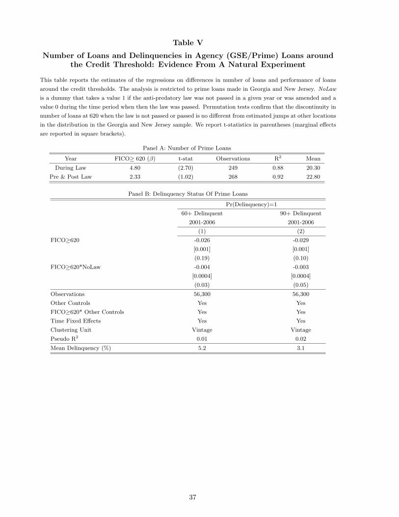
Table V

Number of Loans and Delinquencies in Agency (GSE/Prime) Loans aroundthe Credit Threshold: Evidence From A Natural Experiment

This table reports the estimates of the regressions on differences in number of loans and performance of loans

around the credit thresholds. The analysis is restricted to prime loans made in Georgia and New Jersey. NoLaw

is a dummy that takes a value 1 if the anti-predatory law was not passed in a given year or was amended and a

value 0 during the time period when then the law was passed. Permutation tests confirm that the discontinuity in

number of loans at 620 when the law is not passed or passed is no different from estimated jumps at other locations

in the distribution in the Georgia and New Jersey sample. We report t-statistics in parentheses (marginal effects

are reported in square brackets).

Panel A: Number of Prime Loans

Year FICO≥ 620 (β) t-stat Observations R2 Mean

During Law 4.80 (2.70) 249 0.88 20.30

Pre & Post Law 2.33 (1.02) 268 0.92 22.80

Panel B: Delinquency Status Of Prime Loans

Pr(Delinquency)=1

60+ Delinquent 90+ Delinquent

2001-2006 2001-2006

(1) (2)

FICO≥620 -0.026 -0.029

[0.001] [0.001]

(0.19) (0.10)

FICO≥620*NoLaw -0.004 -0.003

[0.0004] [0.0004]

(0.03) (0.05)

Observations 56,300 56,300

Other Controls Yes Yes

FICO≥620* Other Controls Yes Yes

Time Fixed Effects Yes Yes

Clustering Unit Vintage Vintage

Pseudo R2 0.01 0.02

Mean Delinquency (%) 5.2 3.1

37

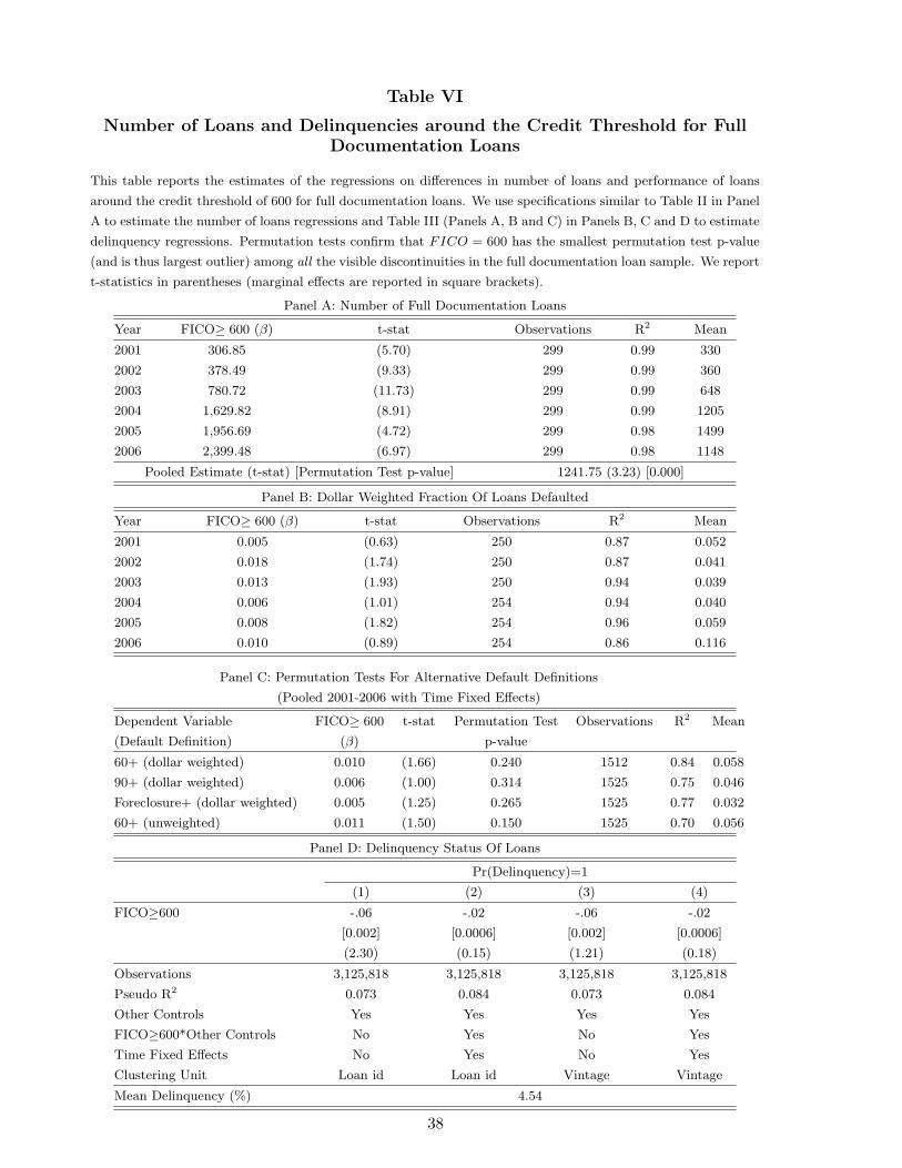
Table VI

Number of Loans and Delinquencies around the Credit Threshold for FullDocumentation Loans

This table reports the estimates of the regressions on differences in number of loans and performance of loans

around the credit threshold of 600 for full documentation loans. We use specifications similar to Table II in Panel

A to estimate the number of loans regressions and Table III (Panels A, B and C) in Panels B, C and D to estimate

delinquency regressions. Permutation tests confirm that FICO = 600 has the smallest permutation test p-value

(and is thus largest outlier) among all the visible discontinuities in the full documentation loan sample. We report

t-statistics in parentheses (marginal effects are reported in square brackets).

Panel A: Number of Full Documentation Loans

Year FICO≥ 600 (β) t-stat Observations R2 Mean

2001 306.85 (5.70) 299 0.99 330

2002 378.49 (9.33) 299 0.99 360

2003 780.72 (11.73) 299 0.99 648

2004 1,629.82 (8.91) 299 0.99 1205

2005 1,956.69 (4.72) 299 0.98 1499

2006 2,399.48 (6.97) 299 0.98 1148

Pooled Estimate (t-stat) [Permutation Test p-value] 1241.75 (3.23) [0.000]

Panel B: Dollar Weighted Fraction Of Loans Defaulted

Year FICO≥ 600 (β) t-stat Observations R2 Mean

2001 0.005 (0.63) 250 0.87 0.052

2002 0.018 (1.74) 250 0.87 0.041

2003 0.013 (1.93) 250 0.94 0.039

2004 0.006 (1.01) 254 0.94 0.040

2005 0.008 (1.82) 254 0.96 0.059

2006 0.010 (0.89) 254 0.86 0.116

Panel C: Permutation Tests For Alternative Default Definitions

(Pooled 2001-2006 with Time Fixed Effects)

Dependent Variable FICO≥ 600 t-stat Permutation Test Observations R2 Mean

(Default Definition) (β) p-value

60+ (dollar weighted) 0.010 (1.66) 0.240 1512 0.84 0.058

90+ (dollar weighted) 0.006 (1.00) 0.314 1525 0.75 0.046

Foreclosure+ (dollar weighted) 0.005 (1.25) 0.265 1525 0.77 0.032

60+ (unweighted) 0.011 (1.50) 0.150 1525 0.70 0.056

Panel D: Delinquency Status Of Loans

Pr(Delinquency)=1

(1) (2) (3) (4)

FICO≥600 -.06 -.02 -.06 -.02

[0.002] [0.0006] [0.002] [0.0006]

(2.30) (0.15) (1.21) (0.18)

Observations 3,125,818 3,125,818 3,125,818 3,125,818

Pseudo R2 0.073 0.084 0.073 0.084

Other Controls Yes Yes Yes Yes

FICO≥600*Other Controls No Yes No Yes

Time Fixed Effects No Yes No Yes

Clustering Unit Loan id Loan id Vintage Vintage

Mean Delinquency (%) 4.54

38

0.001.002.003Density

400

500

600

700

800

900

FIC

O

FIC

O D

istr

ibut

ion

US

Pop

ulat

ion

(200

4)

Fig

ure

1:FIC

OD

istr

ibut

ion

(US

Pop

ulat

ion)

Fig

ure

1pre

sents

the

FIC

Odis

trib

uti

on

inth

eU

.S.popula

tion

for

2004.

This

data

isfr

om

an

anonym

ous

cred

itbure

au

whic

hass

ure

sus

that

the

data

exhib

its

sim

ilar

patt

erns

duri

ng

the

oth

eryea

rsofour

sam

ple

.T

he

FIC

Odis

trib

uti

on

acr

oss

the

popula

tion

issm

ooth

,so

the

num

ber

ofpro

spec

tive

borr

ower

sin

the

loca

lvic

inity

ofa

giv

encr

edit

score

issi

milar.

39

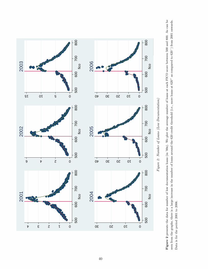
01234

500

600

700

800

fico

2001

0246

500

600

700

800

fico

2002

051015

500

600

700

800

fico

2003

0102030

500

600

700

800

fico

2004

010203040

500

600

700

800

fico

2005

010203040

500

600

700

800

fico

2006

Fig

ure

2:N

umbe

rof

Loan

s(L

owD

ocum

enta

tion

)

Fig

ure

2pre

sents

the

data

for

num

ber

oflo

wdocu

men

tati

on

loans

(in

’00s)

.W

eplo

tth

eav

erage

num

ber

oflo

ans

at

each

FIC

Osc

ore

bet

wee

n500

and

800.

As

can

be

seen

from

the

gra

phs,

ther

eis

ala

rge

incr

ease

inth

enum

ber

oflo

ans

aro

und

the

620

cred

itth

resh

old

(i.e

.,m

ore

loans

at

620+

as

com

pare

dto

620−

)fr

om

2001

onw

ard

s.

Data

isfo

rth

eper

iod

2001

to2006.

40

51015

500

600

700

800

fico

2001

51015

500

600

700

800

fico

2002

51015

500

600

700

800

fico

2003

51015

500

600

700

800

fico

2004

51015

500

600

700

800

fico

2005

51015

500

600

700

800

fico

2006

Fig

ure

3:In

tere

stRat

es(L

owD

ocum

enta

tion

)

Fig

ure

3pre

sents

the

data

for

inte

rest

rate

(in

%)

on

low

docu

men

tati

on

loans.

We

plo

tav

erage

inte

rest

rate

son

loans

at

each

FIC

Osc

ore

bet

wee

n500

and

800.

As

can

be

seen

from

the

gra

phs,

ther

eis

no

change

inin

tere

stra

tes

aro

und

the

620

cred

itth

resh

old

(i.e

.,m

ore

loans

at

620+

as

com

pare

dto

620−

)fr

om

2001

onw

ard

s.

Data

isfo

rth

eper

iod

2001

to2006.

41

050100

500

600

700

800

fico

2001

050100

500

600

700

800

fico

2002

050100

500

600

700

800

fico

2003

050100

500

600

700

800

fico

2004

050100

500

600

700

800

fico

2005

050100

500

600

700

800

fico

2006

Fig

ure

4:Lo

an-to-

Val

ue(L

owD

ocum

enta

tion

)

Fig

ure

4pre

sents

the

data

for

loan-t

o-v

alu

era

tio

(in

%)

on

low

docu

men

tati

on

loans.

We

plo

tav

erage

loan-t

o-v

alu

era

tios

on

loans

at

each

FIC

Osc

ore

bet

wee

n500

and

800.

As

can

be

seen

from

the

gra

phs,

ther

eis

no

change

inlo

an-t

o-v

alu

earo

und

the

620

cred

itth

resh

old

(i.e

.,m

ore

loans

at

620+

as

com

pare

dto

620−

)fr

om

2001

onw

ard

s.D

ata

isfo

rth

eper

iod

2001

to2006.

42

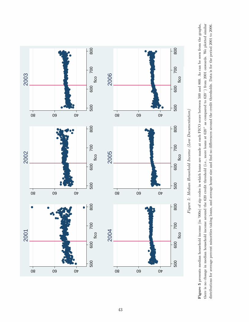
406080

500

600

700

800

fico

2001

406080

500

600

700

800

fico

2002

406080

500

600

700

800

fico

2003

406080

500

600

700

800

fico

2004

406080

500

600

700

800

fico

2005

406080

500

600

700

800

fico

2006

Fig

ure

5:M

edia

nH

ouse

hold

Inco

me

(Low

Doc

umen

tation

)

Fig

ure

5pre

sents

med

ian

house

hold

inco

me

(in

’000s)

ofzi

pco

des

inw

hic

hlo

ans

are

made

at

each

FIC

Osc

ore

bet

wee

n500

and

800.

As

can

be

seen

from

the

gra

phs,

ther

eis

no

change

inm

edia

nhouse

hold

inco

me

aro

und

the

620

cred

itth

resh

old

(i.e

.,m

ore

loans

at

620+

as

com

pare

dto

620−

)fr

om

2001

onw

ard

s.W

eplo

tted

sim

ilar

dis

trib

uti

ons

for

aver

age

per

cent

min

ori

ties

takin

glo

ans,

and

aver

age

house

size

and

find

no

diff

eren

ces

aro

und

the

cred

itth

resh

old

s.D

ata

isfo

rth

eper

iod

2001

to2006.

43

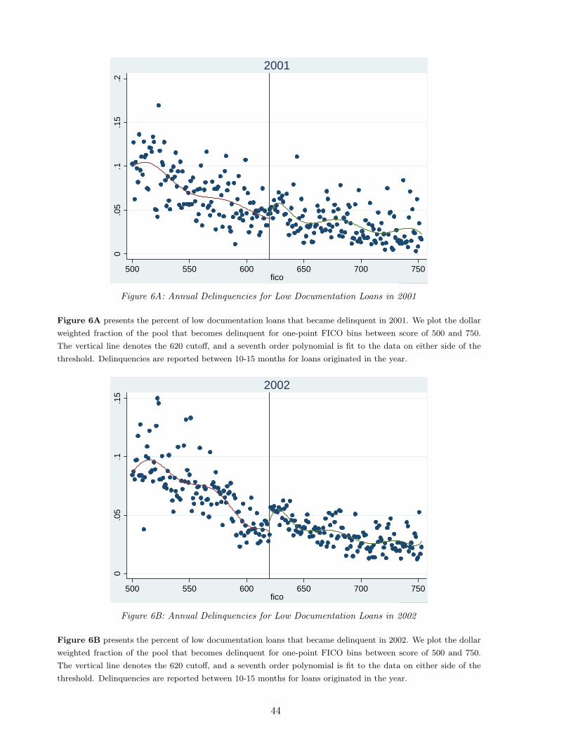
0.0

5.1

.15

.2

500 550 600 650 700 750fico

2001

Figure 6A: Annual Delinquencies for Low Documentation Loans in 2001

Figure 6A presents the percent of low documentation loans that became delinquent in 2001. We plot the dollar

weighted fraction of the pool that becomes delinquent for one-point FICO bins between score of 500 and 750.

The vertical line denotes the 620 cutoff, and a seventh order polynomial is fit to the data on either side of the

threshold. Delinquencies are reported between 10-15 months for loans originated in the year.

0.0

5.1

.15

500 550 600 650 700 750fico

2002

Figure 6B: Annual Delinquencies for Low Documentation Loans in 2002

Figure 6B presents the percent of low documentation loans that became delinquent in 2002. We plot the dollar

weighted fraction of the pool that becomes delinquent for one-point FICO bins between score of 500 and 750.

The vertical line denotes the 620 cutoff, and a seventh order polynomial is fit to the data on either side of the

threshold. Delinquencies are reported between 10-15 months for loans originated in the year.

44

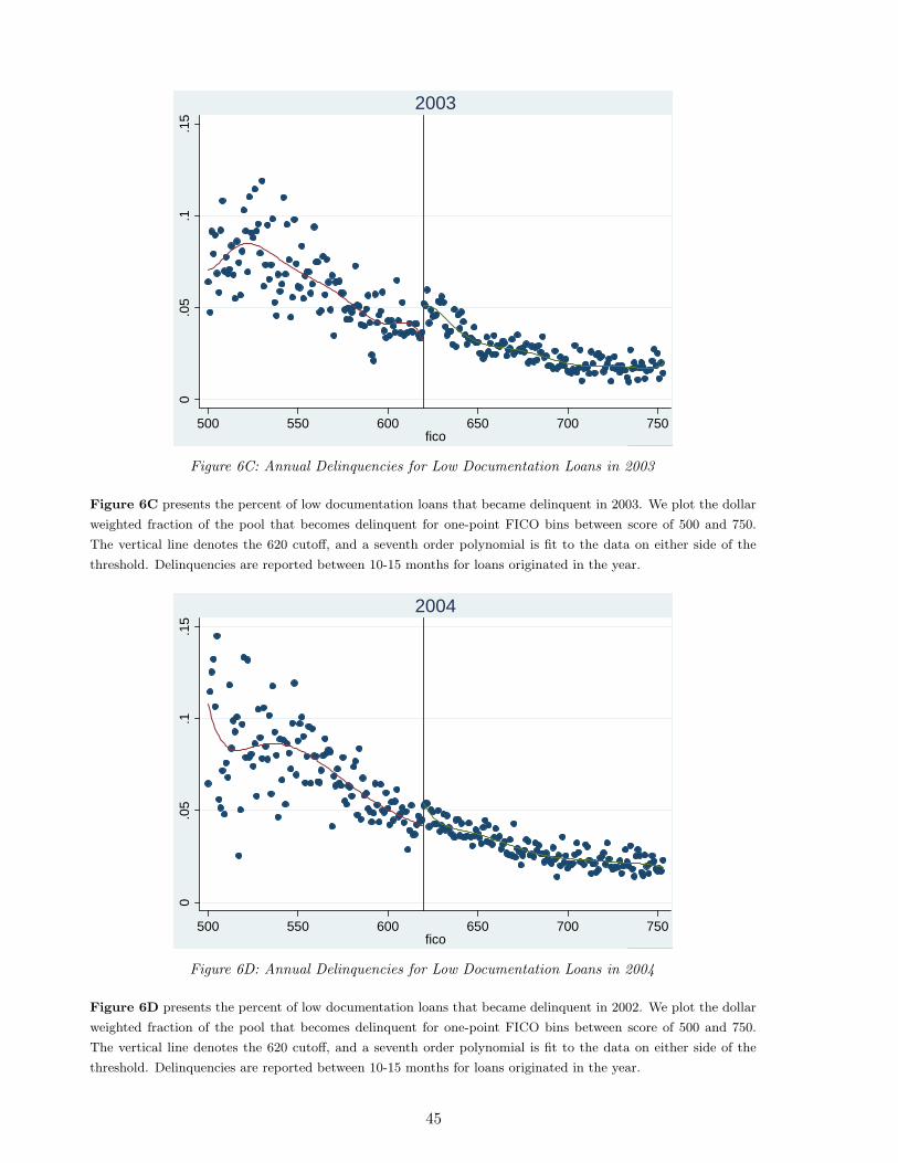
0.0

5.1

.15

500 550 600 650 700 750fico

2003

Figure 6C: Annual Delinquencies for Low Documentation Loans in 2003

Figure 6C presents the percent of low documentation loans that became delinquent in 2003. We plot the dollar

weighted fraction of the pool that becomes delinquent for one-point FICO bins between score of 500 and 750.

The vertical line denotes the 620 cutoff, and a seventh order polynomial is fit to the data on either side of the

threshold. Delinquencies are reported between 10-15 months for loans originated in the year.

0.0

5.1

.15

500 550 600 650 700 750fico

2004

Figure 6D: Annual Delinquencies for Low Documentation Loans in 2004

Figure 6D presents the percent of low documentation loans that became delinquent in 2002. We plot the dollar

weighted fraction of the pool that becomes delinquent for one-point FICO bins between score of 500 and 750.

The vertical line denotes the 620 cutoff, and a seventh order polynomial is fit to the data on either side of the

threshold. Delinquencies are reported between 10-15 months for loans originated in the year.

45

0.0

5.1

.15

.2

500 550 600 650 700 750fico

2005

Figure 6E: Annual Delinquencies for Low Documentation Loans in 2005

Figure 6E presents the percent of low documentation loans that became delinquent in 2005. We plot the dollar

weighted fraction of the pool that becomes delinquent for one-point FICO bins between score of 500 and 750.

The vertical line denotes the 620 cutoff, and a seventh order polynomial is fit to the data on either side of the

threshold. Delinquencies are reported between 10-15 months for loans originated in the year.

.05

.1.1

5.2

.25

.3

500 550 600 650 700 750fico

2006

Figure 6F: Annual Delinquencies for Low Documentation Loans in 2006

Figure 6F presents the percent of low documentation loans that became delinquent in 2006. We plot the dollar

weighted fraction of the pool that becomes delinquent for one-point FICO bins between score of 500 and 750.

The vertical line denotes the 620 cutoff, and a seventh order polynomial is fit to the data on either side of the

threshold. Delinquencies are reported between 10-15 months for loans originated in the year.

46

0%2%4%6%8%10%

12%

14%

12

34

56

78

910

1112

1314

1516

1718

1920

2122

2324

Loan

Age

( M

onth

s)

Delinquency (%)61

5-61

9 (6

20-)

620-

624

(620

+)

Fig

ure

7:D

elin

quen

cies

for

Low

Doc

umen

tation

Loan

s(2

001-

2006

)

Fig

ure

7pre

sents

the

per

cent

oflo

wdocu

men

tati

on

loans

(dollar

wei

ghte

d)

that

bec

am

edel

inquen

tfo

r2001

to2006.

We

track

loans

intw

oFIC

Obuck

ets

–615-6

19

(620−

)in

dott

edblu

eand

620-6

24

(620+)

inre

d–

from

thei

rori

gin

ati

on

date

and

plo

tth

eav

erage

loans

that

bec

om

edel

inquen

tea

chm

onth

aft

erth

eori

gin

ati

on

date

.

As

can

be

seen

,th

ehig

her

cred

itsc

ore

buck

etdef

ault

sm

ore

than

the

low

ercr

edit

score

buck

etfo

rpost

2000

per

iod.

For

bre

vity,

we

do

not

report

plo

tsse

para

tely

for

each

yea

r.T

he

effec

tssh

own

her

ein

the

poole

d2001-2

006

plo

tare

appare

nt

inev

ery

yea

r.

47

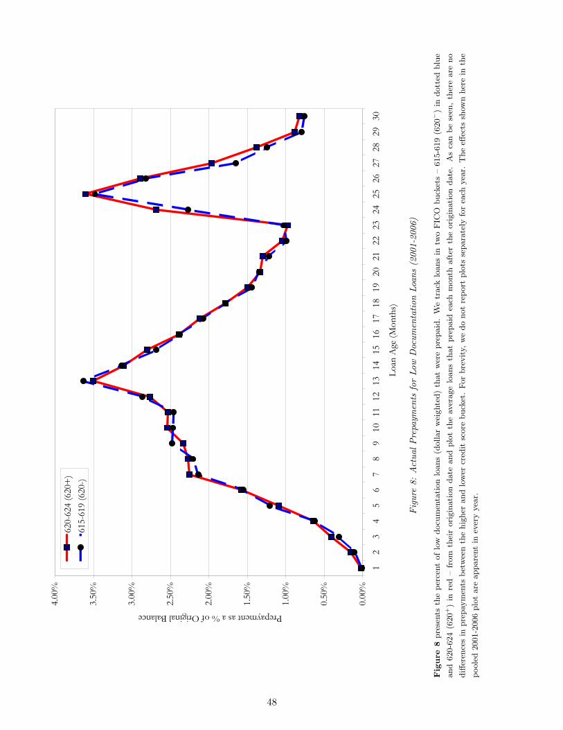
0.00

%

0.50

%

1.00

%

1.50

%

2.00

%

2.50

%

3.00

%

3.50

%

4.00

%

12

34

56

78

910

1112

1314

1516

1718

1920

2122

2324

2526

2728

2930

Loan

Age

(Mon

ths)

Prepayment as a % of Original Balance

620-

624

(620

+)

615-

619

(620

-)

Fig

ure

8:Act

ualPre

paym

ents

for

Low

Doc

umen

tation

Loan

s(2

001-

2006

)

Fig

ure

8pre

sents

the

per

cent

of

low

docu

men

tati

on

loans

(dollar

wei

ghte

d)

that

wer

epre

paid

.W

etr

ack

loans

intw

oFIC

Obuck

ets

–615-6

19

(620−

)in

dott

edblu

e

and

620-6

24

(620+)

inre

d–

from

thei

rori

gin

ati

on

date

and

plo

tth

eav

erage

loans

that

pre

paid

each

month

aft

erth

eori

gin

ati

on

date

.A

sca

nbe

seen

,th

ere

are

no

diff

eren

ces

inpre

pay

men

tsbet

wee

nth

ehig

her

and

low

ercr

edit

score

buck

et.

For

bre

vity,

we

do

not

report

plo

tsse

para

tely

for

each

yea

r.T

he

effec

tssh

own

her

ein

the

poole

d2001-2

006

plo

tare

appare

nt

inev

ery

yea

r.

48

0.1

.2.3

.4D

ensi

ty

0 5 10 15initrate

Kernel density estimate

kdensity initrate

Figure 9A: Dispersion of Interest Rates (Low Documentation)

Figure 9A depicts the Epanechnikov kernel density of interest rate for two FICO groups for low documentation

loans – 620− (615-619) in blue and 620+ (620-624) in red. The bandwidth for the density estimation is selected

using the plug-in formula of Sheather and Jones (1991). The figure shows that the density of interest rates on

loans are similar for both the groups. A Kolmogorov-Smirnov test for equality of distribution functions cannot

be rejected at the 1% level. Data for 2004 is reported here. We find similar patterns for 2001-2006. We do not

report those graphs for brevity.

0.0

2.0

4.0

6.0

8D

ensi

ty

20 40 60 80 100origltv

Kernel density estimate

kdensity origltv

Figure 9B: Dispersion of Loan-to-Value (Low Documentation)

Figure 9B depicts the Epanechnikov kernel density of loan-to-value ratio for two FICO groups for low docu-

mentation loans – 620− (615-619) in blue and 620+ (620-624) in red. The bandwidth for the density estimation

is selected using the plug-in formula of Sheather and Jones (1991). The figure shows that the density of interest

rates on loans are similar for both the groups. A Kolmogorov-Smirnov test for equality of distribution functions

cannot be rejected at the 1% level. Data for 2004 is reported here. We find similar patterns for 2001-2006. We

do not report those graphs for brevity.

49

0%1%2%3%4%5%6%7%8%

01

23

45

67

89

1011

1213

1415

1617

1819

2021

2223

24

Loan

Age

( M

onth

s)

Delinquency (%)61

5-61

9 (6

20-)

620-

624

(620

+)

Fig

ure

10:

Falsifi

cation

Tes

t-

Del

inqu

enci

esfo

rFu

llD

ocum

enta

tion

Loan

sA

roun

dFIC

Oof

620

Fig

ure

10

pre

sents

the

fals

ifica

tion

test

by

exam

inin

gth

eper

cent

of

full

docu

men

tati

on

loans

(dollar

wei

ghte

d)

that

bec

am

edel

inquen

tfo

r2001

to2006.

We

track

loans

intw

oFIC

Obuck

ets

–615-6

19

(620−

)in

dott

edblu

eand

620-6

24

(620+)

inre

d–

from

thei

rori

gin

ati

on

date

and

plo

tth

eav

erage

loans

that

bec

om

edel

inquen

t

each

month

aft

erth

eori

gin

ati

on

date

.A

sca

nbe

seen

,th

ehig

her

cred

itsc

ore

buck

etdef

ault

sle

ssth

an

the

low

ercr

edit

score

buck

etfo

rpost

2000

per

iod.

For

bre

vity,

we

do

not

report

plo

tsse

para

tely

for

each

yea

r.T

he

effec

tssh

own

her

ein

the

poole

d2001-2

006

plo

tsh

owup

for

ever

yyea

r.

50

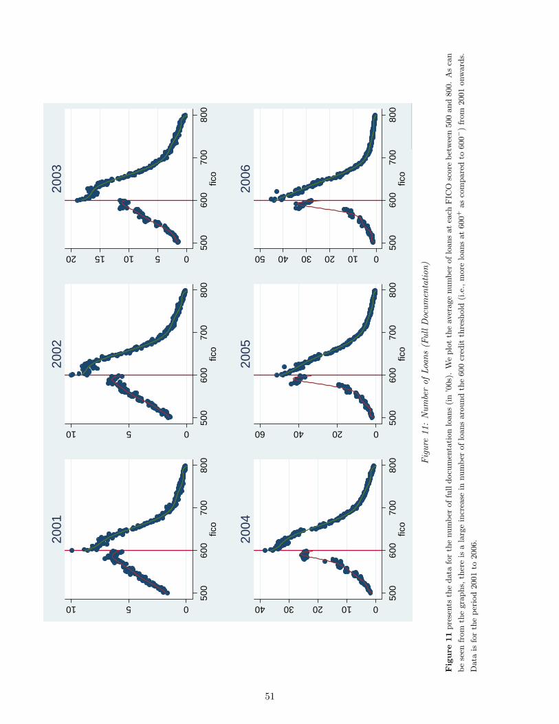
0510

500

600

700

800

fico

2001

0510

500

600

700

800

fico

2002

05101520

500

600

700

800

fico

2003

010203040

500

600

700

800

fico

2004

0204060

500

600

700

800

fico

2005

01020304050

500

600

700

800

fico

2006

Fig

ure

11:

Num

ber

ofLo

ans

(Ful

lD

ocum

enta

tion

)

Fig

ure

11

pre

sents

the

data

for

the

num

ber

offu

lldocu

men

tati

on

loans

(in

’00s)

.W

eplo

tth

eav

erage

num

ber

oflo

ans

at

each

FIC

Osc

ore

bet

wee

n500

and

800.

As

can

be

seen

from

the

gra

phs,

ther

eis

ala

rge

incr

ease

innum

ber

oflo

ans

aro

und

the

600

cred

itth

resh

old

(i.e

.,m

ore

loans

at

600+

as

com

pare

dto

600−

)fr

om

2001

onw

ard

s.

Data

isfo

rth

eper

iod

2001

to2006.

51

0.05.1.15.2

500

550

600

650

700

750

fico

2001

0.05.1.15

500

550

600

650

700

750

fico

2002

0.05.1.15

500

550

600

650

700

750

fico

2003

0.05.1.15

500

550

600

650

700

750

fico

2004

0.05.1.15

500

550

600

650

700

750

fico

2005

.05.1.15.2.25

500

550

600

650

700

750

fico

2006

Fig

ure

12:

Ann

ualD

elin

quen

cies

for

Full

Doc

umen

tation

Loan

s

Fig

ure

12

pre

sents

the

per

cent

of

full

docu

men

tati

on

loans

that

bec

am

edel

inquen

tfo

r2001

to2006.

We

plo

tth

edollar

wei

ghte

dfr

act

ion

of

the

poolth

at

bec

om

es

del

inquen

tfo

rone-

poin

tFIC

Obin

sbet

wee

nsc

ore

of500

and

750.

The

ver

tica

lline

den

ote

sth

e600

cuto

ff,and

ase

ven

thord

erpoly

nom

ialis

fit

toth

edata

on

eith

er

side

ofth

eth

resh

old

.D

elin

quen

cies

are

report

edbet

wee

n10-1

5m

onth

sfo

rlo

ans

ori

gin

ate

din

all

yea

rs.

52

0%1%2%3%4%5%6%7%8%9%10%

12

34

56

78

910

1112

1314

1516

1718

1920

2122

2324

Loan

Age

( M

onth

s)

Delinquency (%)59

5-59

9 (6

00-)

600-

604

(600

+)

Fig

ure

13:

Del

inqu

enci

esfo

rFu

llD

ocum

enta

tion

Loan

s(2

001-

2006

)

Fig

ure

13

pre

sents

the

per

cent

offu

lldocu

men

tati

on

loans

(dollar

wei

ghte

d)

that

bec

am

edel

inquen

tfo

r2001

to2006.

We

track

loans

intw

oFIC

Obuck

ets

–595-5

99

(600−

)in

dott

edblu

eand

600-6

04

(600+)

inre

d–

from

thei

rori

gin

ati

on

date

and

plo

tth

eav

erage

loans

that

bec

om

edel

inquen

tea

chm

onth

aft

erth

eori

gin

ati

on

date

.

As

can

be

seen

,th

ehig

her

cred

itsc

ore

buck

etdef

ault

sm

ore

than

the

low

ercr

edit

score

buck

etfo

rpost

2000

per

iod.

For

bre

vity,

we

do

not

report

plo

tsse

para

tely

for

each

yea

r.T

he

effec

tssh

own

her

ein

the

poole

d2001-2

006

plo

tsh

owup

for

ever

yyea

r.

53

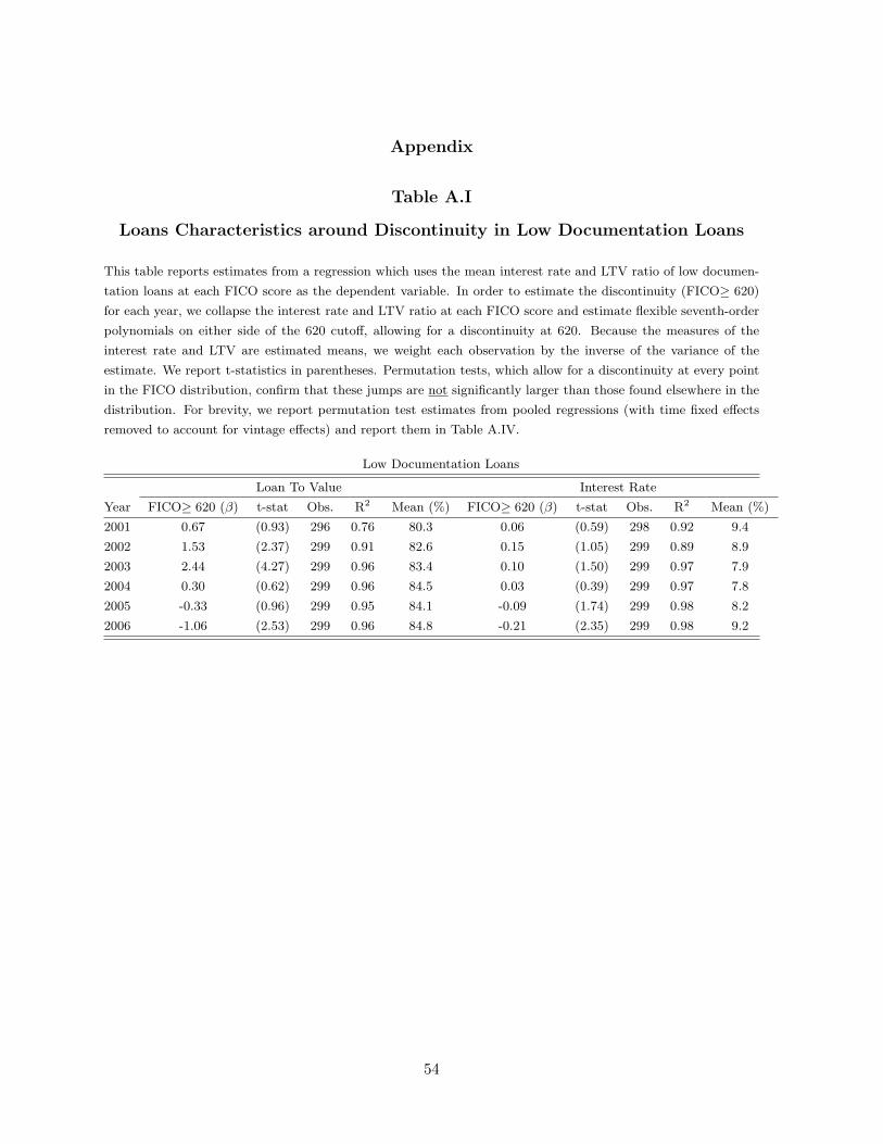
Appendix

Table A.I

Loans Characteristics around Discontinuity in Low Documentation Loans

This table reports estimates from a regression which uses the mean interest rate and LTV ratio of low documen-

tation loans at each FICO score as the dependent variable. In order to estimate the discontinuity (FICO≥ 620)

for each year, we collapse the interest rate and LTV ratio at each FICO score and estimate flexible seventh-order

polynomials on either side of the 620 cutoff, allowing for a discontinuity at 620. Because the measures of the

interest rate and LTV are estimated means, we weight each observation by the inverse of the variance of the

estimate. We report t-statistics in parentheses. Permutation tests, which allow for a discontinuity at every point

in the FICO distribution, confirm that these jumps are not significantly larger than those found elsewhere in the

distribution. For brevity, we report permutation test estimates from pooled regressions (with time fixed effects

removed to account for vintage effects) and report them in Table A.IV.

Low Documentation Loans

Loan To Value Interest Rate

Year FICO≥ 620 (β) t-stat Obs. R2 Mean (%) FICO≥ 620 (β) t-stat Obs. R2 Mean (%)

2001 0.67 (0.93) 296 0.76 80.3 0.06 (0.59) 298 0.92 9.4

2002 1.53 (2.37) 299 0.91 82.6 0.15 (1.05) 299 0.89 8.9

2003 2.44 (4.27) 299 0.96 83.4 0.10 (1.50) 299 0.97 7.9

2004 0.30 (0.62) 299 0.96 84.5 0.03 (0.39) 299 0.97 7.8

2005 -0.33 (0.96) 299 0.95 84.1 -0.09 (1.74) 299 0.98 8.2

2006 -1.06 (2.53) 299 0.96 84.8 -0.21 (2.35) 299 0.98 9.2

54

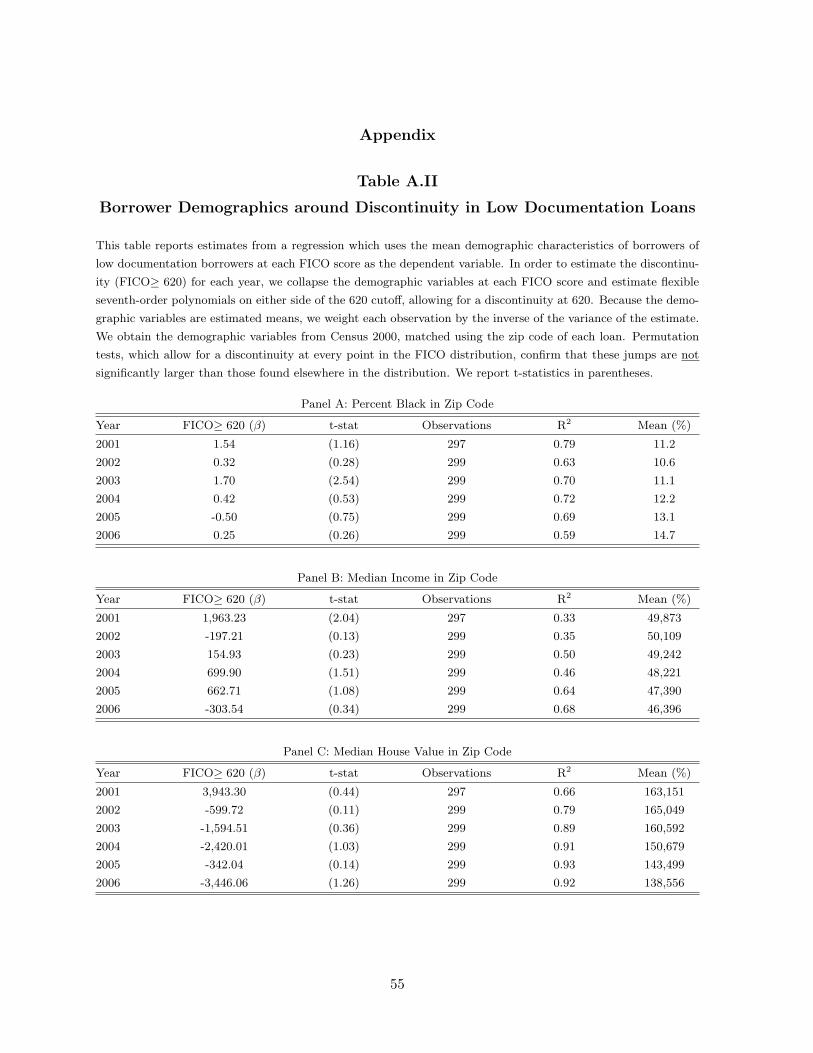
Appendix

Table A.II

Borrower Demographics around Discontinuity in Low Documentation Loans

This table reports estimates from a regression which uses the mean demographic characteristics of borrowers of

low documentation borrowers at each FICO score as the dependent variable. In order to estimate the discontinu-

ity (FICO≥ 620) for each year, we collapse the demographic variables at each FICO score and estimate flexible

seventh-order polynomials on either side of the 620 cutoff, allowing for a discontinuity at 620. Because the demo-

graphic variables are estimated means, we weight each observation by the inverse of the variance of the estimate.

We obtain the demographic variables from Census 2000, matched using the zip code of each loan. Permutation

tests, which allow for a discontinuity at every point in the FICO distribution, confirm that these jumps are not

significantly larger than those found elsewhere in the distribution. We report t-statistics in parentheses.

Panel A: Percent Black in Zip Code

Year FICO≥ 620 (β) t-stat Observations R2 Mean (%)

2001 1.54 (1.16) 297 0.79 11.2

2002 0.32 (0.28) 299 0.63 10.6

2003 1.70 (2.54) 299 0.70 11.1

2004 0.42 (0.53) 299 0.72 12.2

2005 -0.50 (0.75) 299 0.69 13.1

2006 0.25 (0.26) 299 0.59 14.7

Panel B: Median Income in Zip Code

Year FICO≥ 620 (β) t-stat Observations R2 Mean (%)

2001 1,963.23 (2.04) 297 0.33 49,873

2002 -197.21 (0.13) 299 0.35 50,109

2003 154.93 (0.23) 299 0.50 49,242

2004 699.90 (1.51) 299 0.46 48,221

2005 662.71 (1.08) 299 0.64 47,390

2006 -303.54 (0.34) 299 0.68 46,396

Panel C: Median House Value in Zip Code

Year FICO≥ 620 (β) t-stat Observations R2 Mean (%)

2001 3,943.30 (0.44) 297 0.66 163,151

2002 -599.72 (0.11) 299 0.79 165,049

2003 -1,594.51 (0.36) 299 0.89 160,592

2004 -2,420.01 (1.03) 299 0.91 150,679

2005 -342.04 (0.14) 299 0.93 143,499

2006 -3,446.06 (1.26) 299 0.92 138,556

55

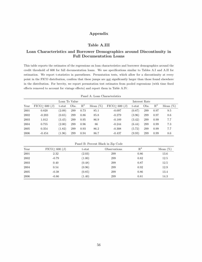
Appendix

Table A.III

Loan Characteristics and Borrower Demographics around Discontinuity inFull Documentation Loans

This table reports the estimates of the regressions on loan characteristics and borrower demographics around the

credit threshold of 600 for full documentation loans. We use specifications similar to Tables A.I and A.II for

estimation. We report t-statistics in parentheses. Permutation tests, which allow for a discontinuity at every

point in the FICO distribution, confirm that these jumps are not significantly larger than those found elsewhere

in the distribution. For brevity, we report permutation test estimates from pooled regressions (with time fixed

effects removed to account for vintage effects) and report them in Table A.IV.

Panel A: Loan Characteristics

Loan To Value Interest Rate

Year FICO≥ 600 (β) t-stat Obs. R2 Mean (%) FICO≥ 600 (β) t-stat Obs. R2 Mean (%)

2001 0.820 (2.09) 299 0.73 85.1 -0.097 (0.87) 299 0.97 9.5

2002 -0.203 (0.65) 299 0.86 85.8 -0.279 (3.96) 299 0.97 8.6

2003 1.012 (3.45) 299 0.95 86.9 -0.189 (3.42) 299 0.99 7.7

2004 0.755 (2.00) 299 0.96 86 -0.244 (6.44) 299 0.99 7.3

2005 0.354 (1.82) 299 0.93 86.2 -0.308 (5.72) 299 0.99 7.7

2006 -0.454 (1.96) 299 0.94 86.7 -0.437 (9.93) 299 0.99 8.6

Panel B: Percent Black in Zip Code

Year FICO≥ 600 (β) t-stat Observations R2 Mean (%)

2001 2.32 (2.03) 299 0.86 13.6

2002 -0.79 (1.00) 299 0.82 12.5

2003 0.40 (0.48) 299 0.87 12.5

2004 0.54 (0.96) 299 0.92 12.9

2005 -0.38 (0.85) 299 0.86 13.4

2006 -0.86 (1.40) 299 0.81 14.3

56

Appendix

Table A.IV

Permutation Test Results For Loan Characteristics in Low and FullDocumentation Loans

This table reports the estimates of the regressions on loan characteristics around the credit threshold of 620 for

low documentation loans and credit threshold of 600 for full documentation loans. We pool the loans across

all years and remove year effects to account for vintage effects. We use specifications similar to Table A.I for

estimation. Permutation tests, which allow for a discontinuity at every point in the FICO distribution, confirm

that these jumps are not significantly larger than those found elsewhere in the distribution. We report p-values

from these tests in the table.

Panel A: Low Documentation Loan Characteristics

Interest Loan To Value Debt To Income Prepayment Actual CLTV

Rate Ratio Ratio Penalty Prepayments Ratio

Pooled FICO≥ 620 (β) 0.02 0.54 0.42 -0.016 -0.0004 0.05

t-stat 0.32 1.40 1.25 1.23 0.44 0.73

Permutation Test p-value 0.90 0.46 0.32 0.55 0.84 0.96

Panel B: Full Documentation Loan Characteristics

Interest Loan To Value Debt To Income Prepayment Actual CLTV

Rate Ratio Ratio Penalty Prepayments Ratio

Pooled FICO≥ 620 (β) 0.39 -0.26 0.68 0.008 -0.0009 0.17

t-stat 1.63 1.91 1.83 0.73 1.51 0.39

Permutation Test p-value 0.20 0.07 0.11 0.45 0.35 0.62

57