Dictionary learning - from local towards global and adaptive

Dictionary learning - from local towards global and adaptive

Marie Christine Pali [email protected]

Karin Schnass [email protected]

Department of Mathematics

University of Innsbruck

Technikerstraße 13

6020 Innsbruck, Austria

Abstract

This paper studies the convergence behaviour of dictionary learning via the IterativeThresholding and K-residual Means (ITKrM) algorithm. On one hand it is proved thatITKrM is a contraction under much more relaxed conditions than previously necessary.On the other hand it is shown that there seem to exist stable fixed points that do not cor-respond to the generating dictionary, which can be characterised as very coherent. Basedon an analysis of the residuals using these bad dictionaries, replacing coherent atoms withcarefully designed replacement candidates is proposed. In experiments on synthetic datathis outperforms random or no replacement and always leads to full dictionary recovery.Finally the question how to learn dictionaries without knowledge of the correct dictionarysize and sparsity level is addressed. Decoupling the replacement strategy of coherent orunused atoms into pruning and adding, and slowly carefully increasing the sparsity level,leads to an adaptive version of ITKrM. In several experiments this adaptive dictionarylearning algorithm is shown to recover a generating dictionary from randomly initialiseddictionaries of various sizes on synthetic data and to learn meaningful dictionaries on imagedata.

Keywords: dictionary learning, sparse coding, sparse component analysis, IterativeThresholding and K-residual Means (ITKrM), replacement, adaptive dictionary learning,parameter estimation.

1. Introduction

The goal of dictionary learning is to decompose a data matrix Y = (y1, . . . , yN ), whereyn ∈ Rd, into a dictionary matrix Φ = (ϕ1, . . . , ϕK), where each column also referred to asatom is normalised, ‖ϕk‖2 = 1 and a sparse coefficient matrix X = (x1, . . . , xN ),

Y ≈ ΦX and X sparse. (1)

The compact data representation provided by a dictionary can be used for data restora-tion, such as denoising or reconstruction from incomplete information, [12, 27, 29] anddata analysis, such as blind source separation, [14, 26, 22, 23]. Due to these applica-tions dictionary learning is of interest to both the signal processing community, whereit is also known as sparse coding, and the independent component analysis (ICA) andthe blind source separation (BSS) community, where it is also known as sparse compo-nent analysis. It also means that there are not only many algorithms to choose from,

1

[14, 3, 13, 23, 26, 28, 45, 29, 38, 31], but also that theoretical results have started to accu-mulate, [17, 46, 4, 1, 40, 41, 18, 6, 5, 43, 47, 48, 9, 35]. As our reference list grows moreincomplete every day, we point to the surveys [36, 42] as starting points for digging intoalgorithms and theory, respectively.One way to concretise the abstract formulation of the dictionary learning problem in (1) isto formulate it as optimisation programme. For instance, choosing a sparsity level S and adictionary size K, we define XS to be the set of all columnwise S-sparse coefficient matrices,DK to be the set of all dictionaries with K atoms and for some p ≥ 1 try to find

argminΨ∈DK ,X∈XS

∑n

‖yn −Ψxn‖p2. (2)

Unfortunately this problem is highly non-convex and as such difficult to solve even in thesimplest and most commonly used case p = 2. However, randomly initialised alternatingprojection algorithms, which alternate between (trying to) find the best dictionary Ψ, basedon coefficients X, and the best coefficients X, based on a dictionary Ψ, such as K-SVD (KSingular Value Decompositions) for p = 2, [3], and ITKrM (Iterative Thresholding and Kresidual Means) related to p = 1, [43], tend to be very successful on synthetic data - usuallyrecovering 90 to 100% of all atoms - and to provide useful dictionaries on image data.Apart from needing both the sparsity level and the dictionary size as input, the maindrawback of these algorithms is that - assuming that the data Y is synthesized from agenerating dictionary Φ and randomly drawn S-sparse coefficients X - they have almost no(K-SVD) or comparatively weak (ITKrM) theoretical dictionary recovery guarantees. Thisis in sharp contrast to more involved algorithms, which - given the correct S,K - have gobalrecovery guarantees but due to their computational complexity can at best be used in smalltoy examples, [4, 2, 6].There are some interesting exceptions. In [5] Arora et. al. propose an initialisation strategy,that can be used to decide the dictionary size, and several alternating projection algorithmsfor local refinement, which in combination are proven to recover any well-behaved dictionary.The alternating projection algorithms are very similar in spirit to ITKrM, and we believethat all are our results on the contractive areas of ITKrM can easily be transferred tothem. In [47, 48], Sun, Qu and Wright study an algorithm based on gradient descent witha Newton trust region method to escape saddle points and prove recovery if the generatingdictionary is a basis. In [35], Qu et. al. study an `4-norm opimisation programme withspherical constraints for overcomplete dictionary learning. They show that every localminimizer is close to an atom of the target dictionary and that around every saddle pointis a large region with negative curvature. These results together with several results inmachine learning which prove that non-convex problems can be well behaved, meaning alllocal minima are global minima, give rise to hope that a similar result can be proved forlearning overcomplete dictionaries via alternating projection.Contribution: In this paper we first study the contractive areas of ITKrM and show thatthe algorithm contracts towards the generating dictionary under much relaxed conditionscompared to those from [43]. We then have a closer a look at experiments where the learneddictionaries do not coincide with the generating dictionary. These spurious dictionaries,which at least experimentally are fixed points, have a very special structure that violatesthe theoretical conditions for contractivity, that is, they contain two nearly identical atoms.

2

Unfortunately, these experimental findings indicate that for alternating projection methodsnot all fixed points correspond to the generating dictionary.However, based on an analysis of the residuals at dictionaries with the discovered structure,we develop a strategy for finding good candidates to replace coherent atoms. With the helpof these replacement candidates, we then tackle one of the most challenging problems indictionary learning - the automatic choice of the sparsity level S and the dictionary size K.This leads to a version of ITKrM that adapts both the sparsity level and the dictionary sizein each iteration. Synthetic experiments show that the resulting algorithm is able recover agenerating dictionary without prescribing its size or the sparsity level even in the presenceof noise and outliers. Complementary experiments on image data further show that thealgorithm learns sensible dictionaries even in practice, where several synthetic assumptionssuch as homogeneous use of all atoms are unlikely to hold.Organisation: In the next section we summarise our notational conventions and introducethe sparse signal model on which all our theoretical results are based. In Section 3 wefamiliarise the reader with the ITKrM algorithm and existing convergence results. Weanalyse the limitations of existing proofs, develop strategies to overcome them and provethat ITKrM is a contraction towards the generating dictionary on an area much larger thanindicated by the convergence radius in [43]. To see whether the non-contractive areas areonly an artefact of our proof strategy, we conduct several small experiments. These showthat indeed there are fixed points of ITKrM, which are not equivalent to the generatingdictionary through reordering and sign flips and violate our conditions for contractivity;in particular, they are very coherent. In Section 4 we analyse the residuals at such baddictionaries and use those insights to develop a strategy for learning good replacementcandidates for coherent atoms. The resulting algorithm is then tested and compared torandom replacement on synthetic data.In Section 5 we then address the big problem how to learn dictionaries without beinggiven the generating sparsity level and dictionary size. This is done by slowly increasingthe sparsity level and by decoupling the replacement strategy into separate pruning of thedictionary and adding of promising replacement candidates. Numerical experiments showthat the resulting algorithm can indeed recover the generating dictionary from initialisationswith various sizes on synthetic data and learn meaningful dictionaries on image data.In the last section we will sketch how the concepts leading to adaptive ITKrM can beextended to other algorithms such as K-SVD or MOD. Finally, based on a discussion of ourresults, we will map out future directions of research.

2. Notations and Sparse Signal Model

Before we hit the strings, we will fine tune our notation and introduce some definitions.Usually subscripted letters will denote vectors with the exception of ε, α, ω, where they arenumbers, for instance xn ∈ RK vs. εk ∈ R, however, it should always be clear from thecontext what we are dealing with.For a matrix M we denote its (conjugate) transpose by M? and its Moore-Penrose pseudo-inverse by M †. We denote its operator norm by ‖M‖2,2 = max‖x‖2=1 ‖Mx‖2 and its Frobe-

nius norm by ‖M‖F = tr(M?M)1/2, remember that we have ‖M‖2,2 ≤ ‖M‖F .We consider a dictionary Φ a collection of K unit norm vectors φk ∈ Rd, ‖φk‖2 = 1. By

3

abuse of notation we will also refer to the d×K matrix collecting the atoms as its columnsas the dictionary, that is, Φ = (φ1, . . . φK). The maximal absolute inner product betweentwo different atoms is called the coherence µ(Φ) of a dictionary, µ(Φ) = maxk 6=j |〈φk, φj〉|.By ΦI we denote the restriction of the dictionary to the atoms indexed by I, that is,ΦI = (φi1 , . . . , φiS ), ij ∈ I, and by P (ΦI) the orthogonal projection onto the span of the

atoms indexed by I, that is, P (ΦI) = ΦIΦ†I . Note that in case the atoms indexed by I are

linearly independent we have Φ†I = (Φ?IΦI)

−1Φ?I . We also define Q(ΦI) to be the orthogonal

projection onto the orthogonal complement of the span of ΦI , that is, Q(ΦI) = Id−P (ΦI),where Id is the identity operator (matrix) in Rd.(Ab)using the language of compressed sensing we define δI(Φ) as the smallest number suchthat all eigenvalues of Φ?

IΦI are included in [1− δI(Φ), 1 + δI(Φ)] and the isometry con-stant δS(Φ) of the dictionary as δS(Φ) := max|I|≤S δI(Φ). When clear from the context wewill usually omit the reference to the dictionary. For more details on isometry constantssee for instance [8].For a (sparse) signal y =

∑k φkxk we will refer to the indices of the S coefficients with

largest absolute magnitude as the S-support of y. Again, we will omit the reference to thesparsity level S if clear from the context.To keep the sub(sub)scripts under control we denote the indicator function of a set Vby χ(V, ·), that is χ(V, v) is one if v ∈ V and zero else. The set of the first S integers weabbreviate by S = 1, . . . , S.We define the distance of a dictionary Ψ to a dictionary Φ as

d(Φ,Ψ) := maxk

min`‖φk ± ψ`‖2 = max

kmin`

√2− 2|〈φk, ψ`〉|. (3)

Note that this distance is not a metric since it is not symmetric. For example, if Φ is thecanonical basis and Ψ is defined by ψi = φi for i ≥ 3, ψ1 = (e1+e2)/

√2, and ψ2 =

∑i φ1/

√d

then we have d(Φ,Ψ) = 1/√

2 while d(Ψ,Φ) =√

2− 2/√d. The advantage is that this

distance is well defined also for dictionaries of different sizes. A symmetric distancebetween two dictionaries Φ,Ψ of the same size could be defined as the maximal distancebetween two corresponding atoms, that is,

ds(Φ,Ψ) := minp∈P

maxk‖φk ± ψp(k)‖2, (4)

where P is the set of permutations of 1, . . . ,K. The distances are equivalent wheneverthere exists a permutation p such that after rearrangement, the cross-Gram matrix Φ?Ψis diagonally dominant, that is, mink |〈φk, ψk〉| > maxk 6=j |〈φk, ψj〉|. Since the main as-sumption for our results will be such a diagonal dominance we will state them in termsof the easier to calculate asymmetric distance and assume that Ψ is already signed andrearranged in a way that d(Φ,Ψ) = maxk ‖φk − ψk‖2. We then use the abbreviationsαmin = mink |〈φk, ψk〉| and αmax = maxk |〈φk, ψk〉|. The maximal absolute inner productbetween two non-corresponding atoms will be called the cross-coherence µ(Φ,Ψ) of thetwo dictionaries, µ(Φ,Ψ) = maxk 6=j |〈φk, ψj〉|.We will also use the following decomposition of a dictionary Ψ into a given dictionary Φand a perturbation dictionary Z. If d(Ψ,Φ) = ε we set ‖ψk−φk‖2 = εk, where by definition

4

maxk εk = ε. We can then find unit vectors zk with 〈φk, zk〉 = 0 such that

ψk = αkφk + ωkzk, for, αk := 1− ε2k/2 and ωk := (ε2

k − ε4k/4)

12 . (5)

Note that if the cross-Gram matrix Φ?Ψ is diagonally dominant we have αmin = mink αk,αmax = maxk αk and d(Ψ,Φ) =

√2− 2αmin.

2.1 Sparse signal model

As basis for our results we use the following signal model, already used in [40, 41, 43]. Givena d×K dictionary Φ, we assume that the signals are generated as

y =Φx+ r√1 + ‖r‖22

, (6)

where x ∈ RK is a sparse coefficient sequence and r ∈ Rd is some noise. We assume that ris a centered subgaussian vector with parameter ρ, that is, E(r) = 0 and for all vectors v themarginals 〈v, r〉 are subgaussian with parameter ρ, meaning they satisfy E(et〈v,r〉) ≤ et2ρ2/2

for all t > 0.To model the coefficient sequences x we first assume that there is a measure νc on a subsetC of the positive, non increasing sequences with unit norm, meaning for c ∈ C we havec(1) ≥ c(2) . . . ≥ c(K) > S and ‖c‖2 = 1. A coefficient sequence x is created by drawing asequence c according to νc, and both a permutation p and a sign sequence σ uniformly atrandom and setting x = xc,p,σ, where xc,p,σ(k) = σ(k)c(p(k)). The signal model then takesthe form

y =Φxc,p,σ + r√

1 + ‖r‖22. (7)

Using this model it is quite simple to incorporate sparsity via the measure νc. To modelapproximately S-sparse signals we require that the S largest absolute coefficients, meaningthose inside the support I = p−1(S), are well balanced and much larger than the remainingones outside the support. Further, we need that the expected energy of the coefficientsoutside the support is relatively small and that the sparse coefficients are well separatedfrom the noise. Concretely we require that almost νc-surely we have

c(1)

c(S)≤ γdyn,

c(S + 1)

c(S)≤ γgap,

‖c(Sc)‖2c(1)

≤ γapp andρ

c(S)≤ γρ. (8)

We will refer to the worst case ratio between coefficients inside the support, γdyn, as dynamic(sparse) range and to the worst case ratio between coefficients outside the support to thoseinside the support, γgap, as the (sparse) gap. Since for a noise free signal the expectedsquared sparse approximation error is

E(‖∑k/∈I

σ(k)c(p(k))φk‖22) = ‖c(Sc)‖22,

we will call γapp the relative (sparse) approximation error. Finally, γρ is called the noise to(sparse) coefficient ratio.

5

Algorithm 3.1: ITKrM (one iteration)

Input: Ψ, Y, S ; // dictionary, signals, sparsity

Initialise: Ψ = 0 ;

foreach n do

Itn = arg maxI:|I|=S ‖Ψ?Iyn‖1 ; // thresholding

an = yn − P (ΨItn)yn ; // residual

foreach k ∈ Itn doψk ← ψk +

[an + P (ψk)yn

]· sign(〈ψk, yn〉) ; // atom update

end

end

Ψ←(ψ1/‖ψ1‖2, . . . , ψK/‖ψK‖2

); // atom normalisation

Output: Ψ

Apart from these worst case bounds we will also use three other signal statistics,

γ1,S := Ec (‖c(S)‖1)) , γ2,S := Ec(‖c(S)‖22

), Cr := Er

(1√

1 + ‖r‖22

). (9)

The constant γ1,S helps to characterise the average size of the sparse coefficients, γ1,S =E(|xi| : i ∈ I) · S ≤

√S, while γ2,S characterises the average sparse approximation quality,

γ2,S = E(‖ΦIxI‖22) ≤ 1. The noise constant can be bounded by

Cr ≥1− e−d√1 + 5dρ2

, (10)

and for large ρ approaches the signal-to-noise ratio, C2r ≈ 1

dρ2 ≈E(‖Φx‖22)

E(‖r‖22), see [41] for details.

To get a better feeling for all the involved constants, we will calculate them for the caseof perfectly sparse signals where c(i) = 1/

√S for i ≤ S and c(i) = 0 else. We then have

γdyn = 1, γgap = 0 and γapp = 0 as well as γ1,S =√S and γ2,S = 1. In the case of noiseless

signals we have Cr = 1 and γρ = 0. In the case of Gaussian noise the noise-to-coefficientratio is related to the signal-to-noise ratio via SNR = S/(γ2

ρd).

3. Global behaviour patterns of ITKrM

The iterative thresholding and K residual means algorithm (ITKrM) was introduced in [43]as modification of its much simpler predecessor ITKsM, which uses signal means insteadof residual means. As can be seen from the summary in Algorithm 3.1 each signal can beprocessed and discarded, thus making the algorithm suitable for a sequential version andparallelisation. The determining factors for the computational complexity are the matrixvector products Ψ?yn between the current estimate of the dictionary Ψ and the signals,O(dKN), and the projections P (ΨItn

)yn. If computed with maximal numerical stabilitythese would have an overall cost O(S2dN), corresponding to the QR decompositions of ΨItn

.However, since usually the achievable precision in the learning is limited by the number of

6

available training signals rather than the numerical precision, it is computationally moreefficient to precompute the Gram matrix Ψ?Ψ and calculate the projections less stably viathe eigenvalue decompositions of Ψ?

ItnΨItn

, corresponding to an overall costO(S3N). Anothergood property of the ITKrM algorithm is that it is proven to converge locally to a generatingdictionary. This means that if the data is homogeneously S-sparse in a dictionary Φ, whereS . µ−2, and we initialise with a dictionary Ψ within radius O(1/

√S), d(Ψ,Φ) . 1/

√S,

then ITKrM using N = O(K logK) samples in each iteration will converge to the generatingdictionary, [43]. In simulations on synthetic data ITKrM shows even better convergencebehaviour. Concretely, if the atoms of the generating dictionary are perturbed with vectorszk chosen uniformly at random from the sphere, ψk = αkφk + ωkzk, ITKrM converges alsofor ratios αk : ωk = 1 : 4. For completely random initialisations, ψk = zk, it finds between90% and 100% of the atoms - depending on the noise and sparsity level.Last but not least, ITKrM is not just a pretty toy with theoretical guarantees but on imagedata produces dictionaries of the same quality as K-SVD in a fraction of the time, [30].Considering the good practical performance of ITKrM, it is especially frustrating that weonly get a convergence radius of size O(1/

√S), while for its simpler cousin ITKsM, which

when initialised randomly performs much worse both on synthetic and image data, we canprove a convergence radius of size O(1/

√logK). Therefore, in the next section we will take

a closer look at the two algorithms and the differences in the convergence proofs. This willallow us to show that ITKrM behaves well on a much larger area.

3.1 Contractive areas of ITKrM

To better understand the idea behind the convergence proofs we first rewrite the atomupdate formula before normalisation, which for one iteration of ITKrM becomes

ψk =∑n:k∈Itn

[Id − P (ΨItn

) + P (ψk)]yn · sign(〈ψk, yn〉),

while for ITKsM we can take the formula above and simply ignore the operators in thesquare brackets. Adding and replacing some terms we expand the sum as

ψk =∑n:k∈Itn

[Id − P (ΨItn

) + P (ψk)]yn · sign(〈ψk, yn〉)

−∑n:k∈In

[Id − P (ΨIn) + P (ψk)

]yn · σn(k)

S1

+∑n:k∈In

[Id − P (ΨIn) + P (ψk)

]yn · σn(k)

−∑n:k∈In

[Id − P (ΦIn) + P (φk)

]yn · σn(k)

S2

+∑n:k∈In

[yn − P (ΦIn)yn + P (φk)yn

]· σn(k).

S3

The term S1 captures the errors thresholding makes in estimating the supports In and signsσn(k) when using the current estimate Ψ. It is (sufficiently) small as long as d(Φ,Ψ) .1/√

logK. The second term S2 captures the difference between the residual using the

7

current estimate and the true dictionary, which is small as long as d(Φ,Ψ) . 1/√S. In

expectation the last term is simply a multiple of the true atom φk, so as long as the numberof signals N is large enough, the last term will concentrate arbitrarily close to φk.As we can see, the main constraint on the convergence radius for ITKrM stems from thesecond term S2, which simply vanishes in case of ITKsM. The problem is that we need toinvert the S × S matrix Ψ?

InΨIn , which is a perturbed version of the matrix Φ?

InΦIn . If

the difference between the dictionaries scales as d(Φ,Ψ) ≈ 1/√S, there exist perturbations

such that Ψ?In

ΨIn is ill conditioned even if Φ?In

ΦIn is not.However, if the current dictionary estimate Ψ is itself a well-conditioned and incoherentmatrix, results on the conditioning of random subdictionaries, [50, 10], tell us that for mostpossible supports In, Ψ?

InΨIn will be close to the identity as long as S . d/ logK. This

means that the term S2 should be small as long as the current estimate Ψ is well-conditionedand incoherent, a property that we can check after each iteration.Therefore, the next question is if also the first term S1 can be controlled for a larger class ofdictionaries Ψ. In our previous estimates we bounded the error per atom by the probabilityof thresholding failing multiplied with the norm bound on the difference of the projections.While simple, this strategy is quite crude as it assigns any error of thresholding to all atoms.However, an atom ψk is only affected by a thresholding error if either k was in the originalsupport or if k is not in the original support but is included in the thresholded support.Further, we can take into account that by perturbing an atom φk, meaning ψk = αkφk+ωkzk,its coherence to one other atom φ` may increase dramatically - to the point of it being abetter approximant than ψ`, that is, if zk ≈ φ` we get 〈φk, φ`〉〈ψk, φ`〉 ≈ 〈ψ`, φ`〉.However, if the original Φ itself is well-conditioned, ψk cannot become coherent to all(many) other atoms.Indeed using both of these ideas we get a refined result characterising the contractive areasof ITKrM. To keep the flow of the paper we will state it in an informal version and referthe reader to Appendix A for the exact statement and its proof.

Theorem 1 Assume that the sparsity level of the training signals scales as S . µ(Φ)−2/ logKand that the number of training signals scales as N ≈ SK logK. Further, assume that thecoherence and operator norm of the current dictionary estimate Ψ satisfy,

µ(Ψ) .1

logKand ‖Ψ‖22,2 .

K

S logK. (11)

If the distance of Ψ to the generating dictionary Φ satisfies either

a) 1√S. d(Ψ,Φ) . 1√

logKor

b) d(Ψ,Φ) & 1√logK

but the cross-Gram matrix Φ?Ψ is diagonally dominant in the sense

that

mink|〈φk, ψk〉| & logK ·max

µ(Φ,Ψ), ‖Φ‖2,2

√S/(K logK)

, (12)

then one iteration of ITKrM will reduce the distance by at least a factor κ < 1, meaning

d(Ψ,Φ) < κ · d(Ψ,Φ).

8

The first part of the theorem simply says that, excluding dictionaries Ψ that are coherentor have large operator norm, ITKrM is a contraction on a ball of radius 1/

√logK around

the generating dictionary Φ. To better understand the second part of the theorem, wehave a closer look at the conditions on the cross-Gram matrix Φ?Ψ in (12). The factthat the diagonal entries have to be larger than ‖Φ‖2,2

√(S logK)/K puts a constraint on

the admissible distance d(Φ,Ψ) via the relation d(Φ,Ψ)2 = 2 − 2 mink |〈φk, ψk〉|. For awell-conditioned dictionary, satisfying ‖Φ‖22,2 ≈ K/d, this means that

d(Φ,Ψ) .

(2− 2

√S logK

d

)1/2

. (13)

Considering that the maximal distance between two dictionaries is√

2, this is a large im-provement over the admissible distance 1/

√logK in a). However, the additional price to

pay is that also the intrinsic condition on the cross-Gram matrix needs to be satisfied,

mink|〈φk, ψk〉| & logK ·max

j 6=k|〈φk, ψj〉|. (14)

This condition captures our intuition that two estimated atoms should not point to thesame generating atom and provides a bound for sufficient separation.One thing that has to be noted about the result above is that it does not guarantee conver-gence of ITKrM since it is only valid for one iteration. To prove convergence of ITKrM, weneed to additionally prove that Ψ inherits from Ψ the properties that are required for beinga contraction, which is part of our future goals. Still, the result goes a long way towardsexplaining the good convergence behaviour of ITKrM.For example, it allows us to briefly sketch why the algorithm always converges in exper-iments where the initial dictionary is a large but random perturbation of a well-behavedgenerating dictionary Φ with coherence µ(Φ) ≈ 1/

√d and operatornorm ‖Φ‖22,2 ≈ K/d. If

ψk = αkφk + ωkzk, where the perturbation vectors zk are drawn uniformly at random fromthe unit sphere orthogonal to φk, then with high probability for all j 6= k we have

|〈φk, zj〉| .√

logK/d and |〈zk, zj〉| .√

logK/d (15)

and consequently for all possible αk

µ(Ψ) .√

4 logK/d and µ(Φ,Ψ) .√

2 logK/d. (16)

Also with high probability the operator norm of the matrix Z = (z1, . . . zK) is bounded by‖Z‖2,2 .

√logK, [49], so that for Ψ we get ‖Ψ‖2,2 .

√K/d+

√logK, again independent

of αk. Comparing these estimates with the requirements of the theorem we see that formoderate sparsity levels, S ≥ logK, we get a contraction whenever

αmin &

√S(logK)2

d⇔ d(Φ,Ψ) .

(2− 2

√S(logK)2

d

)1/2

. (17)

A fully random initialisation will have small coherence and operator norm with high prob-ability. While it is also exponentially more likely to satisfy the cross-coherence property

9

Figure 1: Cross-Gram matrices Ψ?Φ for recovered dictionaries with 2 (left) and 4 (right)missing atoms.

than to be within distance 1/√S or 1/

√logK to the generating dictionary, the absolute

probability of having the cross-coherence property is still very small. This leads to thequestion whether in practice the cross-coherence property is actually necessary for conver-gence. Experiments in the next section will provide evidence that it is practically relevant,in the sense, that whenever ITKrM does not recover the generating dictionary, it producesa dictionary not satisfying the cross-coherence property.

3.2 Bad dictionaries

From [43] we know that ITKrM is most likely to not recover the full dictionary from arandom initialisation when the signals are very sparse (S small) and the noiselevel is small.Since we want to closely inspect the resulting dictionaries, we only run a small experimentin R32, where we try to recover a very incoherent dictionary from 2-sparse vectors1. Thedictionary, containing 48 atoms, consists of the Dirac basis and the first half of the vectorsfrom the Hadamard basis, and as such has coherence µ = 1/

√32 ≈ 0.18. The signals follow

the model in (7), where the coefficient sequences c are constructed by chosing b ∈ [0.9, 1]uniformly at random and setting c1 = 1/

√1 + b2; c2 = bc1 and cj = 0 for j ≥ 3. The

noise is chosen to be Gaussian with variance ρ2 = 1/(16d), corresponding to SNR = 16.Running ITKrM with 20000 new signals per iteration for 25 iterations and 10 differentrandom initialisations we recover 4 times 46 atoms and 6 times 44 atoms. An immediateobservation is that we always miss an even number of atoms. Taking a look at the recovereddictionaries - examples for recovery of 44 and 46 atoms are shown in Figure 3.2 - we see thatthis is due to their special structure; in case of 2n missing atoms, we always observe thatn atoms of the generating dictionary are recovered twice and that n atoms in the learneddictionary are a 1:1 linear combinations of 2 missing atoms from the generating dictionary,respectively.So in the most simple case of 2 missing atoms (after rearranging and sign flipping the atoms

1. All experiments and resulting figures can be reproduced using the matlab toolbox available at https:

//www.uibk.ac.at/mathematik/personal/schnass/code/adl.zip

10

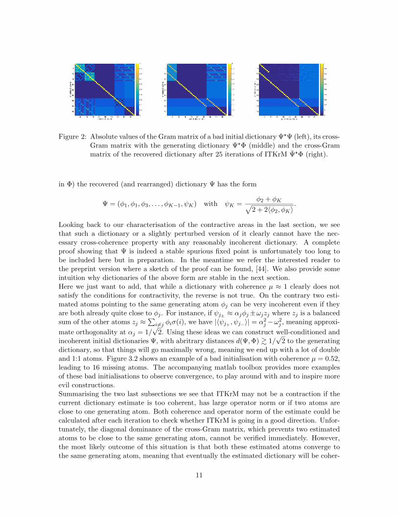
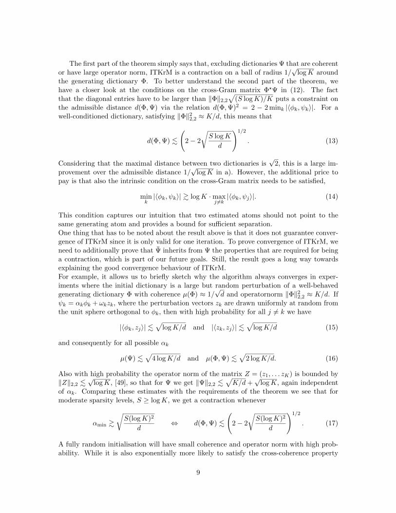
Figure 2: Absolute values of the Gram matrix of a bad initial dictionary Ψ?Ψ (left), its cross-Gram matrix with the generating dictionary Ψ?Φ (middle) and the cross-Grammatrix of the recovered dictionary after 25 iterations of ITKrM Ψ?Φ (right).

in Φ) the recovered (and rearranged) dictionary Ψ has the form

Ψ = (φ1, φ1, φ3, . . . , φK−1, ψK) with ψK =φ2 + φK√

2 + 2〈φ2, φK〉.

Looking back to our characterisation of the contractive areas in the last section, we seethat such a dictionary or a slightly perturbed version of it clearly cannot have the nec-essary cross-coherence property with any reasonably incoherent dictionary. A completeproof showing that Ψ is indeed a stable spurious fixed point is unfortunately too long tobe included here but in preparation. In the meantime we refer the interested reader tothe preprint version where a sketch of the proof can be found, [44]. We also provide someintuition why dictionaries of the above form are stable in the next section.Here we just want to add, that while a dictionary with coherence µ ≈ 1 clearly does notsatisfy the conditions for contractivity, the reverse is not true. On the contrary two esti-mated atoms pointing to the same generating atom φj can be very incoherent even if theyare both already quite close to φj . For instance, if ψj± ≈ αjφj±ωjzj where zj is a balancedsum of the other atoms zj ≈

∑i 6=j φiσ(i), we have |〈ψj+ , ψj−〉| = α2

j −ω2j , meaning approxi-

mate orthogonality at αj = 1/√

2. Using these ideas we can construct well-conditioned andincoherent initial dictionaries Ψ, with abritrary distances d(Ψ,Φ) & 1/

√2 to the generating

dictionary, so that things will go maximally wrong, meaning we end up with a lot of doubleand 1:1 atoms. Figure 3.2 shows an example of a bad initialisation with coherence µ = 0.52,leading to 16 missing atoms. The accompanying matlab toolbox provides more examplesof these bad initialisations to observe convergence, to play around with and to inspire moreevil constructions.Summarising the two last subsections we see that ITKrM may not be a contraction if thecurrent dictionary estimate is too coherent, has large operator norm or if two atoms areclose to one generating atom. Both coherence and operator norm of the estimate could becalculated after each iteration to check whether ITKrM is going in a good direction. Unfor-tunately, the diagonal dominance of the cross-Gram matrix, which prevents two estimatedatoms to be close to the same generating atom, cannot be verified immediately. However,the most likely outcome of this situation is that both these estimated atoms converge tothe same generating atom, meaning that eventually the estimated dictionary will be coher-

11

ent. This suggests that in order to improve the global convergence behaviour of ITKrM,we should control the coherence of the estimated dictionaries. One strategy to incorporateincoherence into ITKrM could be adding a penalty for coherent dictionaries. The maindisadvantages of this strategy, apart from the fact that ITKrM is not straightforwardlyassociated to an optimisation programme, are the computational cost and the fact thatpenalties tend to complicate the high-dimensional landscape of basins of attractions whichfurther complicates convergence. Therefore, we will use a different strategy which allows usto keep the high percentage of correctly recovered atoms and even use the information theyprovide for identifying the missing ones: replacement.

4. Replacement

Replacement of coherent atoms with new, randomly drawn atoms is a simple clean-up stepthat most dictionary learning algorithms based on alternating minimisation, e.g. K-SVD[3], employ additionally in each iteration. While randomly drawing a replacement is cost-efficient and democratic, the drawback is that the new atom converges only very slowly ornot at all to the missing generating atom.To see why a randomly drawn replacement atom is not the best idea and what to do instead,we first have a look at the shape of the signal residuals at one of the bad dictionaries,identified in the last section.

4.1 Learning from bad dictionaries

We start with an analysis of thresholding in case the current dictionary Ψ contains onedouble atom, ψ1 = ψ2 = φ1, and one 1:1 atom, ψK ∝ φ2 +φK ; for the other atoms we haveψk = φk. We will also keep track of what would happen if we replaced one of the doubleatoms with a vector drawn uniformly at random from the unit sphere, which we label ψ0.For simplicity we assume that the signals follow the sparse model in (7) with constantcoefficients ci = 1 for i ≤ S and ci = 0 for i ≥ 0 and no noise, and that 〈φ2, φK〉 ≥ 0. Wealso adopt the notation I`↔k := (I \ `) ∪ k. Note that we have

|〈ψk, φk〉| = 1 for k /∈ 2,Kand |〈ψk, φi〉| ≤ µ for k 6= K, i /∈ 1, 2, k.

We also have |〈ψ2, φ1〉| = 1 as well as

|〈ψK , φ2〉| = |〈ψK , φK〉| =|〈φ2 + φK , φK〉|√

2 + 2〈φ2, φK〉=

√1 + 〈φ2, φK〉

2≥ 1√

2

and |〈ψK , φi〉| =|〈φ2 + φK , φi〉|√

2 + 2〈φ2, φK〉≤ 2µ√

2≤√

2µ for i /∈ 2,K

Since ψ0 is drawn uniformly at random from the d-dimensional unit sphere, we have for anyfixed vector v that

P(|〈ψ0, v〉| ≥ t) ≤ 2 exp

(− t

2d

2

).

12

This means that with very high probability |〈ψ0, φk〉| .√

logK/d for all k.

If we draw a random support I of size S, (a random permutation), then with probability(K−3S

)/(KS

)≈(1− S

K

)3it does not contain 1, 2,K, meaning I∩1, 2,K = ∅. We then have

k ∈ I : |〈ψk, y〉| = |〈ψk, φk〉σkck +∑

i∈I,i 6=k〈ψk, φi〉σici| ≥ 1− (S − 1)µ,

k ∈ Ic \ 0,K : |〈ψk, y〉| = |∑i∈I〈ψk, φi〉σici| ≤ Sµ,

k = K : |〈ψk, y〉| = |∑i∈I〈ψK , φi〉σici| ≤

√2Sµ

k = 0 : |〈ψk, y〉| = |∑i∈I〈ψ0, φi〉σici| ≤ S

√logK/d.

So no matter whether the dictionary contains a double atom or a random replacement atom,thresholding will correctly identify the support, It = I, and the residual will be zero

a = y − P (ΨIt)y = ΦIxI − P (ΦI)ΦIxI = 0.

Next we have a look at supports containing 1 but not 2 or K, meaning I ∩ 1, 2,K = 1.Such a support is drawn with probability

(K−3S−1

)/(KS

)≈ S

K

(1− S

K

)2. As before we get the

following bounds

k ∈ I ∪ 2 : |〈ψk, y〉| ≥ 1− (S − 1)µ,

k ∈ Ic \ 0, 2,K : |〈ψk, y〉| ≤ Sµ,

as well as |〈ψK , y〉| ≤√

2Sµ and |〈ψ0, y〉| ≤ S√

logK/d, which ensures that It ⊆ I ∪ 2.If we are lucky and |〈ψ2, y〉| = |〈ψ1, y〉| = mini∈I |〈ψi, y〉| or in the case of the dictionarywith the random replacement atom, thresholding recovers It = I or It = I1↔2 ≡ I and theresidual is again zero. If we are less lucky, we miss one of the relevant atoms indexed byi ∈ I, meaning It = Ii↔2. In this case the residual will be close to φi,

a = y − P (ΨIt)y = ΦIxI − P (ΦI\i)ΦIxI = xi(φi − P (ΦI\i)φi) ≈ ±φi,

since ‖P (ΦI\i)φi‖2 ≤ µ√S/(1− Sµ). Note that for any fixed i /∈ 1, 2,K, the probability

that both 1, i ⊆ I is bounded by(K−3S−2

)/(KS

)≈ S2

K2

(1− S

K

), so a residual close to φi

appears with probability less than S2

K2 .Finally, we analyse what happens when the support contains K but not 1 or 2, meaning

I ∩ 1, 2,K = K. Again this occurs with probability ≈ SK

(1− S

K

)2. We then have

k ∈ I \ K : |〈ψk, y〉| = |〈ψk, φk〉σkck +∑

i∈I,i 6=k〈ψk, φi〉σici| ≥ 1− (S − 1)µ,

k = K : |〈ψk, y〉| = |〈ψK , φK〉σKcK +∑

i∈I,i 6=K〈ψK , φi〉σici| ≥

1− 2(S − 1)µ√2

,

13

as well as |〈ψ0, y〉| ≤ S√

logK/d and |〈ψk, y〉| ≤ Sµ for all other atoms, which shows thatfor both types of dictionary Ψ (with double or random replacement atom) thresholding willrecover It = I. For the residual we get

a = y − P (ΨIt)y = [Id − P (ΨI)]ΦIxI = xK [Id − P (ΨI)]φK

= xK [Id − P (ΨI)][P (ψK) +Q(ψK)]φK

= xK [Id − P (ΨI)]Q(ψK)φK

≈ ±12(φK − φ2),

where we have used that Q(ψK)φK = φK − 〈ψK , φK〉ψK = 12(φK − φ2) and

‖P (ΨI)Q(ψK)φK‖2 ≤ 12 · ‖Ψ

†I‖2,2 · ‖Ψ

?I(φK − φ2)‖2 ≤ µ ·

√S/(1− 2Sµ).

The analysis of the case I ∩ 1, 2,K = 2 is analogue to the one above and shows thatthe residual again is close to ±1

2(φK − φ2). Summarising our analysis so far, we see that

with probability(1− S

K

)3the residual will be zero (or close to zero in the noisy case), with

probability at most S2

K2 it will be close to φi for each i /∈ 1, 2,K and with probability2SK

(1− S

K

)2it will be close to a scaled version of

ψK′ =φK − φ2√

2− 2〈φ2, φK〉.

Also after covering all supports except those where |I ∩ 1, 2,K| ≥ 2, which together have

probability ≈ 3S2

K2 , we have not encountered a situation, where the randomly chosen atomψ0 would have been picked. Indeed a more detailed analysis to be found in [32] shows thatψ0 only has a chance to be picked if I ∩1, 2,K = 2,K. Moreover, for σ2 = σK we havea = y − P (ΨI\2)y = 0. So even if ψ0 is picked, it will not be pulled in a useful direction.Indeed ψ0 will only be picked and pulled in a good direction if σ2 = −σK and therefore

a = y − P (ΨIt)y ≈ y − P (ΨI\2,K)y ≈ α · ψK′ ,

for some scaling factor α = ±√

2− 2〈φ2, φK〉. This case is also the only case, where wehave the chance of accidentally picking ψ1 or ψ2 and having them distorted in the directionof ψK′ . Note that in case I ∩ 1, 2,K = 1, 2 or 1,K we recover It = I or It = IK↔2

and so a ≈ ±φ2 or a ≈ ±φK , but due to the random signs the pull in these useful directionscancels out, and similarly for 1, 2,K ⊆ I. The intuition why configurations like Ψ arestable is that this case is so rare that ψ1 resp. ψ2 cannot be sufficiently perturbed to changethe behaviour of thresholding in the next iteration.So rather than hoping for the at best unlikely distortion of ψ0 or ψ1/2 towards ψK′ we will usethe fact that most non-zero residuals (or residuals not just consisting of noise) are close toscaled versions of ψK′ and recover ψK′ directly. Indeed a more general analysis, to be foundin [32], shows that for dictionaries containing several double atoms and 1:1 combinations,meaning after rearranging and resigning the dictionaries Φ,Ψ we have ψk = φk for k > 3Las well as

ψ` = ψL+` = φ` and ψ2L+` =φ` + φ2L+`√

2 + 2〈φ`, φ2L+`〉for ` = 1 . . . L,

14

the residuals are 1-sparse in the L complementary 1:1 combinations.

ψc` :=φ` − φ2L+`√

2− 2〈φ`, φ2L+`〉for ` = 1 . . . L.

This suggests to use ITKrM with sparsity level 1, which reduces to ITKsM or line clus-tering, on the residuals to directly recover the 1:1 complements as replacement candidates.Replacing the double atom ψ` by ψc` , in the next iteration it will be serious competition forψ2L+` in the thresholding of all signals containing either φ` or φ2L+`. This iteration willthen create a first imbalance of the ratio between φ` and φ2L+` within one or both of theestimated atoms, making one the more likely choice for φ` and the other the more likelychoice for φ2L+` in the subsequent iteration. There the imbalance will be further increaseduntil a few iterations later we finally have ψ` ≈ φ` and ψ2L+` ≈ φ2L+` or the other wayaround.We can also immediately see the advantages this ITKsM/clustering approach provides overother residual based replacement strategies, such as using the largest residual or usingthe largest principal components or [38, 21]. In the case of noise or outliers, the largestresiduals are most likely to be outliers or pure noise, meaning that this strategy effectivelycorresponds to random replacement. The largest principal components of the residuals onthe other hand, will most likely be a linear combination of several 1:1 complementary atomsand as such less serious competition for the original 1:1 combinations during thresholding.Additionally to lower chances of being picked, they will also need more iterations to deter-mine which one will rotate into which place.After learning enough from bad dictionaries to inspire a promising replacement strategy,the next subsection will deal with its practical implementation.

4.2 Replacement in detail

Now that we have laid out the basic strategy, it remains to deal with all the details. Forinstance, if we have used all replacement candidates after one iteration, after the nextiteration the replacement candidates might not be mature yet, meaning they might nothave converged yet.

Efficient learning of replacement atoms.To solve this problem, observe that the number of replacement candidates, stored in Γ =(γ1, . . . γL), will be much smaller than the dictionary size, L K. Therefore, we need lesstraining signals per iteration to learn the candidates or equivalently we can update Γ morefrequently, meaning we renormalise after each batch of NΓ < N signals and set Γ = Γ. Likethis, every augmented iteration of ITKrM will produce L replacement candidates.

Combining coherent atoms.The next questions concern the actual replacement procedure. Assume we have fixed athreshold µmax for the maximal coherence. If our estimate Ψ contains two atoms whosemutual coherence is above the threshold, |〈ψk, ψk′〉| > µmax, which atom should we replace?One strategy that has been employed for instance in the context of analysis operator learn-ing, [11], is to average the two atoms, that is to set ψnewk = ψk + sign(〈ψk, ψk′〉)ψk′ . Thereasoning is that if both atoms are good approximations to the generating atom φk thentheir average will be an even better approximation. However, if one atom ψk is already

15

a very good approximation to the generating atom ψk ≈ φk while ψk′ is still as far awayas indicated by µmax, that is ψk′ ≈ µmaxφk +

√1− µ2

maxzk, then the averaged atom willbe a worse approximation than ψk and it would be preferable to simply keep ψk. To de-termine which of two coherent atoms is the better approximation, we note that the betterapproximation to φk should be more likely to be selected during thresholding. This meansthat we can simply count how often each atom is contained in the thresholded supportsItn, v(k) = ]n : k ∈ Itn and in case of two coherent atoms keep the more frequently usedone. Based on the value function v we can also employ a weighted merging strategy and setψnewk = v(k)ψk + sign(〈ψk, ψk′〉)v(k′)ψk′ . If both atoms are equally good approximations,then their value functions should be similar and the balanced combination will be a betterapproximation. If one atom is a much better approximation it will be used much more oftenand the merged atom will correspond to this better atom.

Selecting a candidate atom.Having chosen how to combine two coherent atoms, we next need to decide which of ourL replacement candidates we are going to use. To keep the dictionary incoherent, we firstdiscard all candidates γ`, whose maximal coherence with the remaining dictionary atoms islarger than our threshold, that is, maxk |〈γ`, φk〉| ≥ µmax. Note that in a perfectly S-sparsesetting this is not very likely since the residuals we are summing up contain mainly noiseor missing 1:1 complements and therefore add up to noise or the desired 1:1 complements.However it might be a problem if we underestimate the sparsity level in the learning. If weuse S < S, the residuals are still at least S − S sparse in the dictionary, so some of ourreplacement candidates might be near copies of already recovered atoms in the dictionary.To decide which remaining candidate is likely to be the most valuable, we use a countersimilar to the one for the dictionary atoms. However, we have to be more careful heresince every residual is added to one candidate. If the residual contains only noise, whichhappens in most cases, and the candidates are reasonably incoherent to each other, then eachcandidate is equally likely to have its counter increased. This means that the candidate atomthat actually encodes the missing atom (or 1:1 complement) will only be slightly more oftenused than the other candidates. So to better distinguish between good and bad candidates,we additionally employ a threshold τ and set vΓ(`) = ]n : ` = in, |〈γ`, an〉| ≥ τ‖an‖. Todetermine the size of the threshold, observe that for a residual consisting only of Gaussiannoise, a = r, we have for any γ` the bound

P(|〈γ`, r〉| ≥ τ‖r‖2) ≤ 2 exp

(−dτ

2

2

). (18)

which for τ =√

2 log(2K)/d becomes 1/K. This means that the contribution to vΓ(`) fromall the pure noise residuals is at best N/K. On the other hand, with probability S/K,the residual will encode the missing atom or 1:1 complement a ≈ (φi − φj) · |xi|/2. Forreasonable sparsity levels, S . d

4 log(2K) , and signal to noise ratios, the candidate γ` closest

to the missing atom will be picked and should have inner product of the size |〈γ`, a〉| ≈|xi|/2 ≈ 1

2√S& τ‖a‖2. This means that for a good candidate the value function will be

closer to NS/K.The threshold should also help in the earlier mentioned case of underestimating the sparsitylevel. There one could imagine the candidates to be poolings of already recovered atoms,

16

that is, γ` ≈∑

j∈J` ±φj/√|J`|, which are sufficiently incoherent to the dictionary atoms

to pass the coherence test. If the residuals are homogenously S − S sparse in the originaldictionary, the candidate atom γ` will be picked if φj approximates the residual best fora j ∈ J`. If additionally the sets J` are disjoint, atoms corresponding to a bigger atompool are (up to a degree) more likely to be choosen than those corresponding to a smallerpool. The threshold helps favour candidates associated to small pools, which have biggerinner products, since |〈γ`, an〉| ≈ 1/

√S|J`|. This is desirable since the candidate closest to

the missing atom will correspond to a smaller pool. After all, a candidate containing in itspool the missing atom (1:1 complement) will be soon distorted towards this atom since thesparse residual coefficient of the missing atom will be on average larger than those of theother atoms, thus reducing the effective size of the pool.

Dealing with unused atoms.Before implementing our new replacement strategy, let us address another less frequentlyactivated safeguard included in most dictionary learning algorithms: the handling of dic-tionary atoms that are never selected and therefore have a zero update. As in the caseof coherent atoms the standard procedure is replacement of such an atom with a randomredraw, which however comes with the problems discussed above. Fortunately our replace-ment candidates again provide an efficient alternative. If an atom has never been updated,or more generally, if the norm of the new estimator is too small, we simply do not updatethis atom but set the associated value function to zero. After replacing all coherent atomswe then proceed to replace these unused atoms.The combination of all the above considerations leads to the augmented ITKrM algorithm,which is summarised in Algorithm C.1 while the actual procedure for replacing coherentatoms is described in Algorithm C.2, both to be found in Appendix C. With these detailsfixed, the next step is to see how much the invested effort will improve dictionary recovery.

4.3 Numerical Simulations

In this subsection we will verify that replacing coherent atoms improves dictionary recoveryand test whether our strategy improves over random replacement. Our main setup is thefollowing:Generating dictionary: As generating dictionary Φ we use a dictionary of size K = 192in Rd with d = 128, where the atoms are drawn i.i.d. from the unit sphere.(Sparse) training signals: We generate S-sparse training signals according to our signalmodel in (7) as

y =Φxc,p,σ + r√

1 + ‖r‖22. (19)

For every signal a new sequence c is generated by drawing a decay factor q uniformly atrandom in [0.9, 1] and setting ci = cqq

i−1 for i ≤ S and 0 else, where cq := 1−q1−qS so that

‖c‖2 = 1. The noise is centered Gaussian noise with variance ρ2 = (16d)−1, leading to asignal to noise ratio of SNR = 16. We will consider two types of training signals. Thefirst type consists of 6-sparse signals with 5% outliers, that is, we randomly select 5% ofthe sparse signals and replace them with pure Gaussian noise of variance 1/d2. The secondtype consists of 25% 4-sparse signals, 50% 6-sparse signals and 25% 8-sparse signals, where

17

iterations0 20 40 60 80 100

unre

covere

d a

tom

s in %

10-3

10-2

10-1

100

threshold mumax = 0.5

no reprand, delrand, mergerand, addcand, delcand, mergecand, add

iterations0 20 40 60 80 100

unre

covere

d a

tom

s in %

10-3

10-2

10-1

100



iterations0 20 40 60 80 100

unre

covere

d a

tom

s in %

10-3

10-2

10-1

100



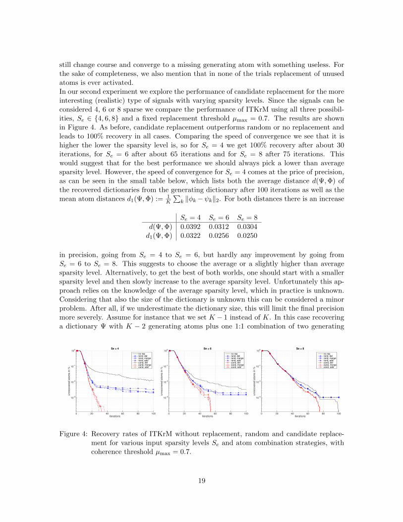
Figure 3: Recovery rates of ITKrM without replacement, random and candidate replace-ment for various coherence thresholds µmax and atom combination strategies.

again 5% are replaced with pure Gaussian noise. In each iteration of ITKrM we use a freshbatch of N = 120000 training signals. Unless specified otherwise, the sparsity level givento the algorithm is Se = 6.Replacement candidates: During every iteration of ITKrM we learn L = blog de = 5replacement candidates using m = blog de = 5 iterations each with NΓ = bN/mc signals.Initialisations: The dictionary Ψ containing K atoms as well as the replacement can-didates are initialised by drawing vectors i.i.d. from the unit sphere. In case of randomreplacement we use the initialisations of the replacement candidates. All our results areaveraged over 20 different initialisations.Replacement thresholds: We will compare the dictionary recovery for various coherencethresholds µmax ∈ 0.5, 0.7, 0.9, and all three combination strategies, adding, deleting andmerging. We also employ an additional safeguard and replace atoms, which have not beenused at all or which have energy smaller than 0.001 before normalisation, if after replace-ment of coherent atoms we have candidate atoms left.Recovery threshold: We use the convention that a dictionary atom φk is recovered ifmaxj |〈φk, ψj〉| ≥ 0.99.The results of our first experiment2, which explores the efficiency of replacement using ourcandidate strategy in comparison to random or no replacement on 6-sparse signals as de-scribed above, are depicted in Figure 3. We can see that for all three considered coherencethresholds µmax ∈ 0.5, 0.7, 0.9, our replacement strategy improves over random or noreplacement. So while after 100 iterations ITKrM without replacement misses about 1%of the atoms and with random replacement about 0.1%, it always finds the full dictionaryafter at worst 55 iterations using the candidate atoms. Contrary to random replacement thecandidate based strategy also does not seem sensitive to the combination method. Anotherobservation is that candidate replacement leads to faster recovery the lower the coherencethreshold is, while the average performance for random replacement is slightly better for thehigher thresholds. This is connected to the average number of replaced atoms in each run,which is around 16 for µmax = 0.5, around 3.8 for µmax = 0.7 and around 0.8 for µmax = 0.9,since for the candidate replacement there is no risk of replacing a coherent atom that might

2. As already mentioned, all experiments can be reproduced using the matlab toolbox available at https:

//www.uibk.ac.at/mathematik/personal/schnass/code/adl.zip

18

still change course and converge to a missing generating atom with something useless. Forthe sake of completeness, we also mention that in none of the trials replacement of unusedatoms is ever activated.In our second experiment we explore the performance of candidate replacement for the moreinteresting (realistic) type of signals with varying sparsity levels. Since the signals can beconsidered 4, 6 or 8 sparse we compare the performance of ITKrM using all three possibil-ities, Se ∈ 4, 6, 8 and a fixed replacement threshold µmax = 0.7. The results are shownin Figure 4. As before, candidate replacement outperforms random or no replacement andleads to 100% recovery in all cases. Comparing the speed of convergence we see that it ishigher the lower the sparsity level is, so for Se = 4 we get 100% recovery after about 30iterations, for Se = 6 after about 65 iterations and for Se = 8 after 75 iterations. Thiswould suggest that for the best performance we should always pick a lower than averagesparsity level. However, the speed of convergence for Se = 4 comes at the price of precision,as can be seen in the small table below, which lists both the average distance d(Ψ,Φ) ofthe recovered dictionaries from the generating dictionary after 100 iterations as well as themean atom distances d1(Ψ,Φ) := 1

K

∑k ‖φk−ψk‖2. For both distances there is an increase

Se = 4 Se = 6 Se = 8

d(Ψ,Φ) 0.0392 0.0312 0.0304d1(Ψ,Φ) 0.0322 0.0256 0.0250

in precision, going from Se = 4 to Se = 6, but hardly any improvement by going fromSe = 6 to Se = 8. This suggests to choose the average or a slightly higher than averagesparsity level. Alternatively, to get the best of both worlds, one should start with a smallersparsity level and then slowly increase to the average sparsity level. Unfortunately this ap-proach relies on the knowledge of the average sparsity level, which in practice is unknown.Considering that also the size of the dictionary is unknown this can be considered a minorproblem. After all, if we underestimate the dictionary size, this will limit the final precisionmore severely. Assume for instance that we set K − 1 instead of K. In this case recoveringa dictionary Ψ with K − 2 generating atoms plus one 1:1 combination of two generating

iterations0 20 40 60 80 100

unre

covere

d a

tom

s in %

10-3

10-2

10-1

100

Se = 4


iterations0 20 40 60 80 100

unre

covere

d a

tom

s in %

10-3

10-2

10-1

100

Se = 6


iterations0 20 40 60 80 100

unre

covere

d a

tom

s in %

10-3

10-2

10-1

100

Se = 8


Figure 4: Recovery rates of ITKrM without replacement, random and candidate replace-ment for various input sparsity levels Se and atom combination strategies, withcoherence threshold µmax = 0.7.

19

atoms leading to d(Ψ,Φ) & 12 is actually the best we can hope for.

Therefore, in the next section we will use our candidate atoms to make the big step towardsadaptive selection of both sparsity level and dictionary size.

5. Adaptive dictionary learning

We first investigate how to adaptively choose the sparsity level for a dictionary of fixed size.

5.1 Adapting the sparsity level

In the numerical simulations of the last section we have seen that the sparsity level S givenas parameter to the ITKrM algorithm influences both the convergence speed and the finalprecision of the learned dictionary.When underestimating the sparsity level, meaning providing Se < S instead of S, the al-gorithm tends to recover the generating dictionary in less iterations than with the truesparsity level. Note also that the computational complexity of an iteration increases withSe, so a smaller sparsity level leads to faster convergence not only in terms of iterationsbut also reduces the computation time per iteration. The advantage of overestimating thesparsity level, Se > S on the other hand, is the potentially higher precision, so the finalerror between the recovered and the generating dictionary (atoms), can be smaller than forthe true sparsity level S. Intuitively this is due to the fact that for Se > S, thresholdingwith the generating dictionary is more likely to recover the correct support, in the sensethat I ⊂ It. For a clean signal, y = ΦIxI this means that the residual is zero, so thatthe estimate of every atom in It, even if not in I, is simply reinforced by itself 〈φi, y〉φi.However, in a noisy situation, y = ΦIxI + r, where the residual has the shape a = QItr theestimate of the additional atom i ∈ It/I is not only reinforced but also disturbed by addingnoise in form of the residual once more than necessary. Depending on the size of the noiseand the inner product this might not always be beneficial to the final estimate. Indeed, wehave seen that for large S, where the smallest coefficients in the support are already quitesmall, overestimating the support does not improve the final precision.To further see that both under- and overestimating the sparsity level comes with risks,assume that we allow S + 1 instead of the true sparsity level S for perfectly sparse, cleansignals. Then any dictionary, derived from the generating dictionary by replacing a pairof atoms (φi, φj) by (φi, φj) = A(φi, φj) for an invertible (well conditioned) matrix A, willprovide perfectly S+ 1-sparse representations to the signals and be a fixed point of ITKrM.Providing S−1 instead of S can have even more dire consequences since we can replace anygenerating atom with a random vector and again have a fixed point of ITKrM. If the originaldictionary is an orthonormal basis and the sparse coefficients have equal size in absolutevalue any such disturbed estimator even gives the same approximation quality. However,in more realistic scenarios, where we have coherence, noise or imbalanced coefficients andtherefore the missing atom has the same probability as the others to be among the S − 1atoms most contributing to a signal, the generating dictionary should still provide the small-est average approximation error. Indeed, whenever we have coherence, noise or imbalancedcoefficients the signals can be interpreted as being 1-sparse (with enormous error and minis-cule gap c(1)/c(2)) in the generating dictionary, so learning with Se = 1 should lead to areasonable first estimate of most atoms. Of course if the signals are not actually 1-sparse

20

this estimate will be somewhere between rough, for small S, and unrecognisable, for largerS, and the question is how to decide whether we should increase Se. If we already had thegenerating dictionary, the simplest way would be to look at the residuals and see how muchwe can decrease their energy by adding another atom to the support. A lower bound forthe decrease of a residual a can be simply estimated by calculating maxk(〈φk, a〉)2.If we have the correct sparsity level and thresholding recovers the correct support It = I,the residual consists only of noise, a = Q(ΦI)(ΦIxI + r) = Q(ΦI)r ≈ r. For a Gaussiannoise vector r and a given threshold θ · ‖r‖2, we now estimate how many of the remainingK − S atoms can be expected to have inner products larger than θ · ‖r‖2 as

E(]k : |〈r, φk〉|2 > θ2 · ‖r‖22

)=∑k

P(|〈r, φk〉|2 > θ2 · ‖r‖22

)< 2(K − S)e−

dθ2

2 . (20)

In particular, setting θ = θK :=√

2 log(4K)/d the expectation above is smaller than 12 .

This means that if we take the empirical estimator of the expectation above, using theapproximation rn ≈ an, we should get

1

N

∑n

]k : |〈an, φk〉|2 > θ2K · ‖an‖22 .

1

2, (21)

which rounds to zero indicating that we have the correct sparsity level.Conversely, if we underestimate the correct sparsity level, Se = S − m for m > 0, thenthresholding can necessarily only recover part of the correct support, It ⊂ I. Denote theset of missing atoms by Im = I/It. The residual has the shape

a = Q(ΦIt)(ΦIxI + r) = Q(ΦIt)(ΦImxIm + r) ≈ ΦImxIm + r

For all missing atoms i ∈ Im the squared inner products are approximately

|〈a, φi〉|2 ≈ (xi + 〈r, φi〉)2.

Assuming well-balanced coefficients, where |xi| ≈ 1/√S and therefore ‖ΦImxIm‖22 ≈ m/S,

a sparsity level S . d2 log(4K) and reasonable noiselevels, this means that with probability

at least 12 we have for all i ∈ Im

|〈a, φi〉|2 & |xi|2 &1

2m(‖ΦImxIm‖22 + ‖r‖22) & θ2

K‖a‖22,

and in consequence

1

N

∑n

]k : |〈an, φk〉|2 > θ2K · ‖an‖22 &

m

2. (22)

This rounds to at least 1, indicating that we should increase the sparsity level.

Based on the two estimates above and starting with sparsity level Se = 1 we should now beable to arrive at the correct sparsity level S. Unfortunately, the indicated update rule for the

21

sparsity level is too simplistic in practice as it relies on thresholding always finding the cor-rect support given the correct sparsity level. Assume that Se = S but thresholding fails torecover for instance one atom, It = Ii↔j . Then we still have a = Q(ΦIt)(xiφi+r) ≈ xiφi+rand |〈φi, a〉|2 & θ2

K‖a‖2. If thresholding constantly misses one atom in the support, for in-stance because the current dictionary estimate is quite coherent, µ 1/

√d, or not yet very

accurate, this will lead to an increase Se = S + 1. However, as we have discussed above,while increasing the sparsity level increases the chances for full recovery by thresholding,it also increases the atom estimation error which decreases the chances for full recovery.Depending on which effect dominates, this could lead to a vicious circle of increasing thesparsity level, which decreases the accuracy leading to more failure of thresholding andincreasing the sparsity level. In order to avoid this risk we should take into account thatthresholding might fail to recover the full support and be able to identify such failure. Fur-ther, we should be prepared to also decrease the sparsity level.The key to these three goals is to also look at the coefficients of the signal approxima-tion. Assume that we are given the correct sparsity level Se = S but recovered It = Ii↔j .Defining Ii→ = I \ i, the corresponding coefficients xIt have the shape,

xIt = Φ†It(ΦIxI + r) = Φ†It(ΦIi→xIi→ + φixi + r)

= (xIi→ , 0) + (Φ?ItΦIt)

−1Φ?It(φixi + r), (23)

meaning |xIt(j)|2 ≤ (µ2|xi|2 + |〈φj , r〉|2)/(1 − µS)2 or even |xIt(j)|2 . µ2|xi|2 + |〈φj , r〉|2.Since the residual is again approximately a ≈ φixi + r, this means that for incoherentdictionaries the coefficient of the wrongly chosen atom is likely to be below the thresholdθ2K‖a‖2, while the one of the missing atom will be above the threshold, so we are likely to

keep the sparsity level the same.Similarly if we overestimate the sparsity level Se = S + 1 and recover an extra atomIt = I←j := I ∪ j, we have a = Q(ΦIt)r ≈ r while the coefficient of the extra atom willbe of size |xIt(j)|2 ≈ |〈φj , r〉|2 < θ2

K‖a‖22. All in all our estimates suggest that we get a

more stable estimate of the sparsity level by averaging the number of coefficients xIt = Φ†Ityand residual inner products (〈φi, a〉)i/∈It that have squared value larger than θ2

K times theresidual energy. However, the last detail we need to include in our considerations is thereason for thresholding failing to recover the full support given the correct sparsity levelin first place. Assume for instance, that the signal does not contain noise, y = ΦIxI butthat the sparse coefficients vary quite a lot in size. We know (from Appendix B or [7]) thatin case of i.i.d. random coefficient signs, P(sign(xi) = 1) = 1/2, the inner products of theatoms inside resp. outside the support concentrate around,

i ∈ I |〈φi,ΦIxI〉| ≈ |xi| ±(∑

k 6=ix2k|〈φi, φk〉|2

)1/2 ≈ |xi| ± µ‖y‖2i /∈ I |〈φi,ΦIxI〉| ≈

(∑kx

2k|〈φi, φk〉|2

)1/2 ≈ µ‖y‖2.This means that thresholding will only recover the atoms corresponding to the Sr-largestcoefficients for Sr < S, that is, Ir = i ∈ I : |xi| & µ‖y‖2. The good news is that thesewill capture most of the signal energy, ‖P (ΦIt)y‖22 ≈ ‖ΦIrxIr‖22 ≈ ‖y‖22, meaning that insome sense the signal is only Sr sparse. It also means that for µ2 ≈ 1/d, we can estimatethe recoverable sparsity level of a given signal as the number of squared coefficients/residual

22

inner products that are larger than

1

d‖P (ΦIt)y‖22 +

2 log(4K)

d‖Q(ΦIt)y‖22. (24)

If Sn is the estimated recoverable sparsity level of signal yn, a good estimate of the overallsparsity level S will be the rounded average sparsity level S = b 1

N

∑n Sne. The correspond-

ing update rule then is to increase Se by one if S > Se, keep it the same if S = Se anddecrease it by one if S < Se, formally

Snewe = Se + sign(S − Se). (25)

To avoid getting lost between numerical and explorative sections we will postpone an algo-rithmic summary to the appendix and testing of our adaptive sparsity selection to Subsec-tion 5.3. Instead we next address the big question how to adaptively select the dictionarysize.

5.2 Adapting the dictionary size

The common denominator of all popular dictionary learning algorithms, from MOD to K-SVD, is that before actually running them one has to choose a dictionary size. This choicemight be motivated by a budget, such as being able to store K atoms and S values persignal, or application specific, that is, the expected number of sources in sparse source sep-aration. In applications such as image restoration K (like S) is either chosen ad hoc orexperimentally with an eye towards computational complexity, and one will usually findd ≤ K ≤ 4d, and S =

√d. If algorithms include some sort of adaptivity of the dictionary

size, this is usually in the form of not updating unused atoms, a rare occurence in noisysituations, and deleting them at the end. Also this strategy can only help if K was chosentoo large but not if it was chosen too small.Underestimating the size of a dictionary obviously prevents recovery of the generating dic-tionary. For instance, if we provide K − 1 instead of K the best we can hope for is adictionary containing K − 2 generating atoms and a 1 : 1 combination of the two missingatoms. The good news is that if we are using a replacement strategy one of the candidateswill encode the 1 : 1 complement, similar to the situation discussed in the last section,where we are given the correct dictionary size but had a double atom.Overestimating the dictionary size does not prevent recovering the dictionary per se, butcan decrease recovery precision, meaning that a bigger dictionary might not actually providesmaller approximation error. To get an intuition what happens in this case assume that weare given a budget of K + 1 instead of K atoms and the true sparsity level S. The mostuseful way to spend the extra budget is to add a 1 : 1 combination of two atoms, whichfrequently occur together, meaning φ0 ∝ φi + hφj for h = sign(〈φi, φj〉). The advantageof the augmented dictionary Ψ = (φ0,Φ) is that some signals are now S − 1 sparse. Thedisadvantage is that Ψ is less stable since the extra atom φ0 will prevent φi or φj to beselected by thresholding whenever they are contained in the support in a 1 : h ratio. Thisdisturbs the averaging process and reduces the final accuracy of both φi and φj .The good news is that the extra atom φ0 is actually quite coherent with the dictionary∣∣〈φ0, φi(j)〉

∣∣ ≥ 1/√

2, so if we have activated a replacement threshold of µmax ≤ 1/√

2, the

23

atom φ0 will be soon replaced, necessarily with another useless atom.This suggests as strategy for adaptively choosing the dictionary size to decouple our re-placement scheme into pruning and adding, which allows to both increase and decrease thedictionary size. We will first have a closer look at pruning.

Pruning atoms.From the replacement strategy we can derive two easy rules for pruning: 1) if two atoms aretoo coherent, delete the less often used one or merge them, 2) if an atom is not used, deleteit. Unfortunately, the second rule is too naive for real world signals, containing amongother imperfections noise, which means also purely random atoms are likely to be used atleast once by mistake. To see how we need to refine the second rule assume again that oursparse signals are affected by Gaussian noise (of a known level), that is, y = ΦIxI + r withE(‖r‖22) = ρ2 and that our current dictionary estimate has the form Ψ = (φ0,Φ), whereφ0 is some vector with admissible coherence to Φ. Whenever φ0 is selected this meansthat thresholding has failed. From the last subsection we also know that we have a goodchance of identifying the failure of thresholding by looking at the coefficients Φ†It(ΦIxI +r).The squared coefficient corresponding to the incorrectly chosen atom φ0 is likely to besmaller than . ‖ΦIxI‖22/d + |〈φ0, r〉|2 while the squared coefficient of a correctly chosenatom i ∈ I ∩ It will be larger than |xi|2 + |〈ψi, r〉|2 & ‖ΦIxI‖22/S + |〈φi, r〉|2 at least half ofthe time. The size of the inner product of any atom with Gaussian noise can be estimatedas

P (|〈φk, r〉| > τ‖r‖2) ≤ 2 exp

(−dτ

2

2

). (26)

Taking again ‖P (ΦIt)y‖2 as estimate for ‖ΦIxI‖2 and ‖a‖2 = ‖Q(ΦIt)y‖2 as estimate for‖r‖2 we can define the refined value function v(k) as the number of times an atom φk hasbeen selected and the corresponding coefficient has squared value larger than ‖P (ΦIt)y‖22/d+τ2‖an‖22. Based on the bound above we can then estimate that for N noisy signals the value

function of the unnecessary or random atom φ0 is bounded by v(0) . 2N exp(−dτ2

2

):= M ,

leading to a natural criterion for deleting unused atoms. Setting for instance τ = θK =√2 log(4K)/d we get M = N/(2d). Alternatively, we can say that in order to accurately

estimate an atom we need M reliable observations and accordingly set the threshold toτ =

√2 log(2N/M)/d.

The advantage of a relatively high threshold τ ≈√

2 log(4K)/d is that in low noise sce-narios, we can also find atoms that are rarely used. The disadvantage is that for highτ the quantities v(·) we have to estimate are relatively small and therefore susceptible torandom fluctuations. In other words, the number of training signals N needs to be largeenough to have sufficient concentration such that for unnecessary atoms the value functionv(·) is actually smaller than M . Another consideration is that at the beginning, when thedictionary estimate is not yet very accurate, also the approximate versions of frequentlyused atoms will not be above the threshold often enough. This risk is further increased ifwe also have to estimate the sparsity level. If Se is still small compared to the true levelS we will overestimate the noise, and even perfectly balanced coefficients 1/

√S will not

yet be above the threshold. Therefore, pruning of the dictionary should only start after anembargo period of several iterations to get a good estimate of the sparsity level and most

24

dictionary atoms.In the replacement section we have also seen that after replacing a double atom with the1:1 complement φi−φj of a 1:1 atom φi +φj , it takes a few iterations for the pair (φi±φj)to rotate into the correct configuration (φi, φj), where they are recovered most of the time.In the case of decoupled pruning and adding, we run the risk of deleting a missing atomor a 1 : 1 complement one iteration after adding it simply because it has not been usedoften enough. Therefore, every freshly added atom should not be checked for its usefulnessuntil after a similar embargo period of several iterations, which brings us right to the nextquestion when to add an atom.

Adding atoms.To see when we should add a candidate atom to the dictionary, we have a look back atthe derivation of the replacement strategy. There we have seen that the residuals are likelyto be either 1-sparse in the missing atoms (or 1:1 complements of the atoms doing thejob of two generating atoms), meaning a ≈ |xi|/2(φi − φj) or in a more realistic situationa ≈ |xi|/2(φi− φj) + r, or zero, which again in the case of noise means a ≈ r. To identify agood candidate atom we observe again that if the residual consists only of (Gaussian) noisewe have for any vector/atom γk

P (|〈γk, r〉| > τΓ‖r‖2) ≤ 2 exp

(−dτ2

Γ

2

). (27)

If on the other hand the residual consists of a missing complement, the correspondingcandidate γ` ≈ (φi − φj)/

√2 should have |〈a, γ`〉| ≈ |xi|/

√2 & τΓ‖a‖2. This means that

we can use a similar strategy as for the dictionary atoms to distinguish between useful anduseless candidates. In the last candidate iteration, using NΓ residuals, we count for eachcandidate atom γk how often it is selected and satisfies |〈γk, a〉| > τΓ‖a‖2. Following thedictionary update and pruning we then add all candidates to the dictionary whose value

function is higher than MΓ = 2NΓ exp(−dτ2

Γ2

)and which are incoherent enough to atoms

already in the dictionary.Now, having dealt with all aspects necessary for making ITKrM adaptive, it is time to testwhether adaptive dictionary learning actually works.

5.3 Experiments on synthetic data

We first test our adaptive dictionary learning algorithm on synthetic data3. The basic setupis the same as in Subsection 4.3. However, one type of training signals will again consistof 4, 6 and 8-sparse signals in a 1:2:1 ratio with 5% outliers, while the second type willconsist of 8, 10 and 12-sparse signals in a 1:2:1 ratio with 5% outliers. Additionally, we willconsider the following settings.The minimal number of reliable observations M for a dictionary atom is set to eitherd, bd log de or b2d log de with corresponding coefficient thresholds τ =

√2 log(2N/M)/d.

For the candidate atoms the minimal number of reliable observations in the 4th (and last)candidate iteration is always set to MΓ = d.

3. Again we want to point all interested in reproducing the experiments to the matlab toolbox available athttps://www.uibk.ac.at/mathematik/personal/schnass/code/adl.zip

25

The sparsity level is adapted after every iteration starting with iteration m = blog de = 5.The initial sparsity level is 1.Promising candidate atoms are added to the dictionary after every iteration, startingagain in the m-th iteration. In the last 3m iterations no more candidate atoms are addedto the dictionary.Coherent dictionary atoms are merged after every iteration, using the threshold µmax =0.7. As weights for the merging we use the value function of the atoms from the most recentiteration.Unused dictionary atoms are pruned after every iteration starting with iteration 2m.An atom is considered unused if in the last m iterations the number of reliable observationshas always been smaller than M . Candidate atoms, freshly added to the dictionary, canonly be deleted because they are unused at least m iterations later. In each iteration atmost bd/5e unused atoms are deleted, with an additional safeguard for very undercompletedictionaries (Ke < d/10) that at most half of all atoms can be deleted.The initial dictionary is chosen to be either of size Ke = d = 128, Ke = 4d = 512 or thecorrect size Ke = K, with the atoms drawn i.i.d. from the unit sphere as before. Figure 5shows the results averaged over 10 trials each using a different initial dictionary.

The first observation is that all our effort paid off and that adaptive dictionary learningworks. For the smaller average sparsity level S = 6, adaptive ITKrM always recovers allatoms of the dictionary and only overshoots and recovers more atoms for M = d. The maindifference in recovery speed derives from the size of the initial dictionary, where a largerdictionary size leads to faster recovery.For the more challenging signals with average sparsity level S = 10, the situation is morediverse. So while the initial dictionary size mainly influences recovery speed but less thefinal number of recovered atoms, the cut off threshold M for the minimal number of reliableobservations is critical for full recovery. So for M = d adaptive ITKrM never recovers thefull dictionary. We can also see that not recovering the full dictionary is strongly correlatedwith overestimating the dictionary size. Indeed, the higher the overestimation factor forthe dictionary size is, the lower is the amount of recovered atoms. For example, for M = d,Ke = 512 the dictionary size is overestimated by a factor 1.5 and only about half of thedictionary atoms are recovered. To see that the situation is not as bad as it seems wehave a look at the average sorted atom recovery error. That is, we sort the recovery errors(d(φk,Ψ))k after 100 iterations in ascending order and average over the number of trials.The resulting curves are depicted in Figure 6. As we can see, overestimating the dictionarysize degrades the recovery in a gentle manner. For the unrecovered atoms in case M = d,Ke = 512, the largest inner product with an atom in the recovered dictionary is below thecut-off threshold of 0.99 which corresponds to an error of size ≈ 0.14 but for almost all ofthem it is still above 0.98 which corresponds to an error of 0.2. Also the oscillating recoverybehaviour for M = bd log(d)e before the final phase, where no more atoms are added, can beexplained by the fact that the worst approximated atoms have average best inner productvery close to 0.99. So, depending on the batch of training signals in each iteration, theirinner product is below or above 0.99 and accordingly they count as recovered or not. Ingeneral, we can see that the more accurate the estimate of the dictionary size is, the betteris the recovery precision of the learned dictionary. This is only to be expected. After all,whenever thresholding picks a superfluous atom instead of a correct atom, the number of

26

S ∈ 4, 6, 8 S ∈ 8, 10, 12

iterations

5 10 15 20 25 30 35

un

reco

ve

red

ato

ms in

%

10-3

10-2

10-1

100

iterations

10 20 30 40 50 60 70 80 90 100

un

reco

ve

red

ato

ms in

%

10-3

10-2

10-1

100

iterations5 10 15 20 25 30 35

rela

tive

siz

e o

f d

ictio

na

ry K

e/K

0.6

0.8

1

1.2

1.4

1.6

1.8

Ke=128, M=dKe=128, M=d*logdKe=128, M=2d*logdKe=192, M=dKe=192, M=d*logdKe=192, M=2d*logdKe=512, M=dKe=512, M=d*logdKe=512, M=2d*logd

iterations10 20 30 40 50 60 70 80 90 100

rela

tive

siz

e o

f d

ictio

na

ry K

e/K

0.6

0.8

1

1.2

1.4

1.6

1.8

Figure 5: Average recovery rates (top row) and dictionary sizes (bottom row) for adaptivedictionary learning based on ITKrM on signals with sparsity S = 4, 6, 8 (leftcolumn) resp. S = 8, 10, 12 (right column) in a 1:2:1 ratio for various initialdictionary sizes Ke and required number of observations per atom M .

observations for the missing atom is reduced and moreover, the residual error added to thecorrectly identified atoms is increased.The relative stability of these spurious atoms can in turn be explained by the fact thatS = 10 is at the limit of admissible sparsity for a generating dictionary with µ(Φ) = 0.32,especially for sparse coefficients with a dynamic range of 0.9S−1 ≈ 2.58. In particular,thresholding is not powerful enough to recover the full support, so the residuals still containseveral generating atoms. This promotes candidate atoms that are a sparse pooling of alldictionary atoms. These poolings again have a good chance to be selected in the thresholdingand to be above the reliability threshold, thus positively reinforcing the effect. A quick lookat the estimated sparsity level as well as the average number of coefficients above thethreshold, or in other words, the average number of (probably) correctly identified atomsin the support, denoted by St, also supports this theory. So for average sparsity level S = 6the estimated sparsity level is Se = 6 = b5.7e and the average number of correctly identifiedatoms is St ≈ 5, regardless of the setting. This is quite close to the average number ofcorrectly identifiable atoms given Se = 6, which is 0.95 ∗ (0.25 ∗ 4 + 0.75 ∗ 6) = 5.225.For average generating sparsity level S = 10 the table below lists Se : St for all settings.We can see that even for the settings where the full dictionary is recovered, the estimated

27

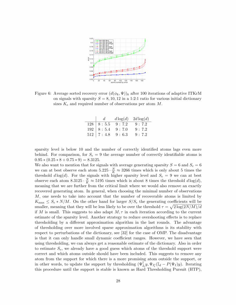
atoms sorted by error0 20 40 60 80 100 120 140 160 180

err

or

0.02

0.04

0.06

0.08

0.1

0.12

0.14

0.16

0.18

0.2

0.22

Ke=128, M=dKe=128, M=d*logdKe=128, M=2d*logdKe=192, M=dKe=192, M=d*logdKe=192, M=2d*logdKe=512, M=dKe=512, M=d*logdKe=512, M=2d*logd

Figure 6: Average sorted recovery error (d(φk,Ψ))k after 100 iterations of adaptive ITKrMon signals with sparsity S = 8, 10, 12 in a 1:2:1 ratio for various initial dictionarysizes Ke and required number of observations per atom M .

d d log(d) 2d log(d)

128 8 : 5.5 9 : 7.2 9 : 7.2192 8 : 5.4 9 : 7.0 9 : 7.2512 7 : 4.8 9 : 6.3 9 : 7.2

sparsity level is below 10 and the number of correctly identified atoms lags even morebehind. For comparison, for Se = 9 the average number of correctly identifiable atoms is0.95 ∗ (0.25 ∗ 8 + 0.75 ∗ 9) = 8.3125.We also want to mention that for signals with average generating sparsity S = 6 and Se = 6we can at best observe each atom 5.225 · NK ≈ 3266 times which is only about 5 times thethreshold d log(d). For the signals with higher sparsity level and Se = 9 we can at bestobserve each atom 8.3125 · NK ≈ 5195 times which is about 8 times the threshold d log(d),meaning that we are further from the critical limit where we would also remove an exactlyrecovered generating atom. In general, when choosing the minimal number of observationsM , one needs to take into account that the number of recoverable atoms is limited byKmax ≤ Se ∗ N/M . On the other hand for larger S/Se the generating coefficients will besmaller, meaning that they will be less likely to be over the threshold τ =

√2 log(2N/M)/d

if M is small. This suggests to also adapt M, τ in each iteration according to the currentestimate of the sparsity level. Another strategy to reduce overshooting effects is to replacethresholding by a different approximation algorithm in the last rounds. The advantageof thresholding over more involved sparse approximation algorithms is its stability withrespect to perturbations of the dictionary, see [32] for the case of OMP. The disadvantageis that it can only handle small dynamic coefficient ranges. However, we have seen thatusing thresholding, we can always get a reasonable estimate of the dictionary. Also in orderto estimate Se, we already have a good guess which atoms of the threshold support werecorrect and which atoms outside should have been included. This suggests to remove anyatom from the support for which there is a more promising atom outside the support, orin other words, to update the support by thresholding (Ψ†Ity,ΨIct

(Id − P (ΨI)y). Iteratingthis procedure until the support is stable is known as Hard Thresholding Pursuit (HTP),

28

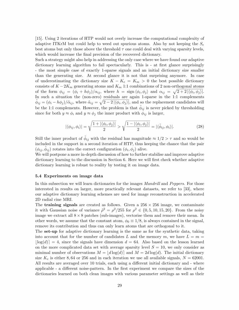
[15]. Using 2 iterations of HTP would not overly increase the computational complexity ofadaptive ITKrM but could help to weed out spurious atoms. Also by not keeping the Sebest atoms but only those above the threshold τ one could deal with varying sparsity levels,which would increase the final precision of the recovered dictionary.Such a strategy might also help in addressing the only case where we have found our adaptivedictionary learning algorithm to fail spectacularly. This is - at first glance surprisingly- the most simple case of exactly 1-sparse signals and an initial dictionary size smallerthan the generating size. At second glance it is not that surprising anymore. In caseof underestimating the dictionary size K − Ke = Km > 0 the best possible dictionaryconsists of K−2Km generating atoms and Km 1:1 combinations of 2 non-orthogonal atomsof the form φij = (φi + hφj)/αij , where h = sign 〈φi, φj〉 and αij =

√2 + 2 |〈φi, φj〉|.

In such a situation the (non-zero) residuals are again 1-sparse in the 1:1 complementsφij = (φi − hφj)/αij , where αij =

√2− 2 |〈φi, φj〉|, and so the replacement candidates will

be the 1:1 complements. However, the problem is that φij is never picked by thresholdingsince for both y ≈ φi and y ≈ φj the inner product with φij is larger,

|〈φij , φi〉| =√

1 + |〈φi, φj〉|2

>

√1− |〈φi, φj〉|

2= |〈φij , φi〉|. (28)

Still the inner product of φij with the residual has magnitude ≈ 1/2 > τ and so would beincluded in the support in a second iteration of HTP, thus keeping the chance that the pair(φij , φij) rotates into the correct configuration (φi, φj) alive.We will postpone a more in-depth discussion of how to further stabilise and improve adaptivedictionary learning to the discussion in Section 6. Here we will first check whether adaptivedictionary learning is robust to reality by testing it on image data.

5.4 Experiments on image data

In this subsection we will learn dictionaries for the images Mandrill and Peppers. For thoseinterested in results on larger, more practically relevant datasets, we refer to [33], whereour adaptive dictionary learning schemes are used for image reconstruction in accelerated2D radial cine MRI.The training signals are created as follows. Given a 256 × 256 image, we contaminateit with Gaussian noise of variance ρ2 = ρ2/255 for ρ2 ∈ 0, 5, 10, 15, 20. From the noisyimage we extract all 8× 8 patches (sub-images), vectorise them and remove their mean. Inother words, we assume that the constant atom, φ0 ≡ 1/8, is always contained in the signal,remove its contribution and thus can only learn atoms that are orthogonal to it.The set-up for adaptive dictionary learning is the same as for the synthetic data, takinginto account that for the number of candidates L and the memory m, we have L = m =blog(d)e = 4, since the signals have dimension d = 64. Also based on the lesson learnedon the more complicated data set with average sparsity level S = 10, we only consider asminimal number of observations M = bd log(d)e and M = 2d log(d). The initial dictionarysize Ke is either 8, 64 or 256 and in each iteration we use all available signals, N = 62001.All results are averaged over 10 trials, each using a different initial dictionary and - whereapplicable - a different noise-pattern. In the first experiment we compare the sizes of thedictionaries learned on both clean images with various parameter settings as well as their

29

iterations10 20 30 40 50 60 70 80 90 100

dic

tionary

siz

e

0

20

40

60

80

100

120

140

160

180

200m, M=d*log(d), Ke=8m, M=d*log(d), Ke=64m, M=d*log(d), Ke=256m, M=2d*log(d), Ke=8m, M=2d*log(d), Ke=64m, M=2d*log(d), Ke=256p, M=d*log(d), Ke=8p, M=d*log(d), Ke=64p, M=d*log(d), Ke=256p, M=2d*log(d), Ke=8p, M=2d*log(d), Ke=64p, M=2d*log(d), Ke=256

sparsity level S1 2 3 4 5 6 7 8 9 10

rela

tive M

SE

0

0.005

0.01

0.015

0.02

0.025

0.03

0.035

0.04m, M=d*log(d), Ke=64m, M=2d*log(d), Ke=64p, M=d*log(d), Ke=64p, M=2d*log(d), Ke=64

Figure 7: Average dictionary sizes for adaptive dictionary learning based on ITKrM on allpatches of Mandrill/Peppers for various initial dictionary sizes Ke and requirednumber of observations per atom M (left). Average sparse approximation errorof all patches of Mandrill/Peppers using OMP and the learned dictionaries withKe = 64 and both choices of M (right).

approximation powers. The approximation power of a dictionary augmented by the flatatom φ0 for a given sparsity level S is measured as ‖Y − Y ‖2F /‖Y ‖2F , where Y = (y1, . . . , yn)and yn is the S-sparse approximation to yn calculated by Orthogonal Matching Pursuit, [34].The results are shown in Figure 7. We can see that as for synthetic data the final size of thelearned dictionary does not depend much on the initial dictionary size, but does depend onthe minimal number of observations. So for M = bd log(d)e the average dictionary size isabout 106 atoms for Mandrill and 55 atoms for Peppers, while for M = 2d log(d) we haveabout 54 atoms on Mandrill and 36 atoms on Peppers. The estimated sparsity level vs.average number of correctly identified atoms for Mandrill is Se = b2.1e = 2 vs. St ≈ 1.5and for Peppers Se = b2.9e = 3 vs. St ≈ 2.25. Comparing the approximation power, wesee that for both images the smaller (undercomplete) dictionaries barely lag behind thelarger dictionaries. The probably most interesting aspect is that despite being smaller, thePeppers-dictionaries lead to smaller error than the Mandrill-dictionaries. This confirms theintuition that the smooth image Peppers has a lot more sparse structure than the texturedimage Mandrill. To better understand why for both images the larger dictionaries do notimprove the approximation much, we have a look at the number of reliable observationsfor each atom in the last trial of Ke = 64 in Figure 8. The corresponding dictionaries forMandrill/Peppers can be found in Figures 9/10.

We can see that for both images the number of times each atom is observed stronglyvaries. If we interpret the relative number of observations as probability of an atom tobe used, the first ten atoms are more than 10 times more likely to be used/observed thanthe last ten atoms. This accounts for the fact that by increasing the threshold for theminimal number of observations, we reduce the dictionary size without much affecting theapproximation power.In our second experiment we learn adaptive dictionaries on Mandrill contaminated withGaussian noise of variance ρ2 = ρ2/255 for σ2 ∈ 5, 10, 15, 20, corresponding to averagepeak signal to noise ratios 34.15, 28.13, 24.61, 22.11. We again compare their sizes and

30

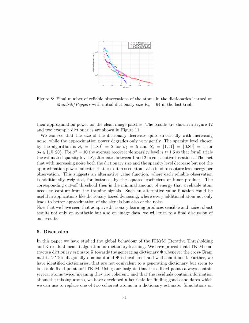
atoms0 20 40 60 80 100

relia

ble

ob

se

rva

tio

ns /

N

10-2

10-1

m, M=d*log(d), Ke=64m, M=2d*log(d), Ke=64p, M=d*log(d), Ke=64p, M=2d*log(d), Ke=64

Figure 8: Final number of reliable observations of the atoms in the dictionaries learned onMandrill/Peppers with initial dictionary size Ke = 64 in the last trial.

their approximation power for the clean image patches. The results are shown in Figure 12and two example dictionaries are shown in Figure 11.

We can see that the size of the dictionary decreases quite drastically with increasingnoise, while the approximation power degrades only very gently. The sparsity level chosenby the algorithm is Se = b1.80e = 2 for σ2 = 5 and Se = b1.11e = b0.89e = 1 forσ2 ∈ 15, 20. For σ2 = 10 the average recoverable sparsity level is ≈ 1.5 so that for all trialsthe estimated sparsity level Se alternates between 1 and 2 in consecutive iterations. The factthat with increasing noise both the dictionary size and the sparsity level decrease but not theapproximation power indicates that less often used atoms also tend to capture less energy perobservation. This suggests an alternative value function, where each reliable observationis additionally weighted, for instance, by the squared coefficient or inner product. Thecorresponding cut-off threshold then is the minimal amount of energy that a reliable atomneeds to capture from the training signals. Such an alternative value function could beuseful in applications like dictionary based denoising, where every additional atom not onlyleads to better approximation of the signals but also of the noise.Now that we have seen that adaptive dictionary learning produces sensible and noise robustresults not only on synthetic but also on image data, we will turn to a final discussion ofour results.

6. Discussion

In this paper we have studied the global behaviour of the ITKrM (Iterative Thresholdingand K residual means) algorithm for dictionary learning. We have proved that ITKrM con-tracts a dictionary estimate Ψ towards the generating dictionary Φ whenever the cross-Grammatrix Ψ?Φ is diagonally dominant and Ψ is incoherent and well-conditioned. Further, wehave identified dictionaries, that are not equivalent to a generating dictionary but seem tobe stable fixed points of ITKrM. Using our insights that these fixed points always containseveral atoms twice, meaning they are coherent, and that the residuals contain informationabout the missing atoms, we have developed a heuristic for finding good candidates whichwe can use to replace one of two coherent atoms in a dictionary estimate. Simulations on

31

Figure 9: Dictionaries learned on Mandrill with initial dictionary size Ke = 64 and requirednumber of observations M = bd log(d)e (top) resp. M = 2d log(d) (bottom).

Figure 10: Dictionaries learned on Peppers with initial dictionary size Ke = 64 and requirednumber of observations M = bd log(d)e (middle) resp. M = 2d log(d) (right).

Figure 11: Dictionaries learned on the Mandrill image contaminated with Gaussian noiseof variance ρ2 = 10/255 (left) and ρ2 = 20/255 (right), initial dictionary sizeKe = 64 and required number of observations M = bd log(d)e.

32

iterations0 20 40 60 80 100

dic

tio

na

ry s

ize

0

20

40

60

80

100

120

140

ρ2 = 0

ρ2 = 5

ρ2 = 10

ρ2 = 15

ρ2 = 20

sparsity level S1 2 3 4 5 6 7 8 9 10

rela

tive

MS

E

0

0.005

0.01

0.015

0.02

0.025

0.03

0.035

0.04

ρ2 = 0

ρ2 = 5

ρ2 = 10

ρ2 = 15

ρ2 = 20

Figure 12: Average dictionary sizes for adaptive dictionary learning based on ITKrM onall patches of the Mandrill image contaminated with Gaussian noise of varianceρ2 = ρ2/255, initial dictionary size Ke = 64 and required number of observationsM = bd log(d)e (left). Corresponding average sparse approximation error of allclean patches of Mandrill using OMP and the learned dictionaries. (right).

synthetic data have shown that replacement using these candidates improved over randomor no replacement, always leading to recovery of the full dictionary.Armed with replacement candidates, we have addressed one of the most challening prob-lems in dictionary learning - how to automatically choose the sparsity level and dictionarysize. We have developed a strategy for adapting the sparsity level from the initial guessSe = 1 and the dictionary size by decoupling replacement into pruning of coherent and un-used atoms and adding of promising candidates. The resulting adaptive dictionary learningalgorithm has been shown to perform very well in recovering a generating dictionary fromrandom initialisations with various sizes on synthetic data with sparsity levels S ≥ 2 andin learning meaningful dictionaries on image data.Note that our strategy for learning replacement candidates and adaptivity can be easilyadapted to any other alternating minimisation algorithm for dictionary learning, such asMOD or K-SVD, [13, 3]. Instead of using ITKsM on the residuals one simply has to usea small scale version with sparsity level S = 1 of the respective algorithm. Preliminaryexperiments on synthetic data show that in the case of K-SVD and MOD this gives verysimilar results, [39]. Interestingly, however, it is much more difficult to stabilise the adaptiveversion of K-SVD on image data. The reason for this seems to be that the more sophisti-cated sparse approximation routine Orthogonal Matching Pursuit (OMP), [34], promotesthe convergence of candidate atoms to high energy subspaces. This leads to a concentrationof many coherent atoms in these subspaces, without proportional increase in the approx-imation quality of the dictionary. These experimental findings are supported by theory,showing that while an excellent choice if the sparsifying dictionary is known, the perfor-mance of OMP rapidly degrades if the sparsifying dictionary is perturbed, [32]. Indeed onsynthetic data without replacement procedures, K-SVD with OMP produces more doubleatoms than ITKrM. However, when using thresholding as sparse approximation proceduresalso for K-SVD and MOD, MOD produces the smallest number of double atoms followedby K-SVD and then ITKrM. With replacement MOD recovers the most accurate dictionary

33

again followed by K-SVD and ITKrM.These observations suggest that the use of more sophisticated algorithms to bridge the gapbetween average sparsity level S and the average number of correctly identified atoms St isonly advisable in the last iterations when the number of atoms is not changed anymore.A promising direction to avoid the concentration of coherent atoms in high energy sub-spaces is to use a different value function for the dictionary atoms. The one proposed hereis based on the assumption that all atoms are used equally often, which for image datawas clearly not the case. Alternatively, the current function could be scaled, that is, everyreliable occurence of an atom is weighted with the squared coefficient which is related tothe signal energy lost without this atom. Preliminary experiments with ITKrM using thisweighted value function and an accordingly scaled cut-off indicate that it indeed helps toremove spurious atoms on synthetic data and leads to smaller dictionaries with the sameapproximation power on image data.Another interesting question, which leads directly to our future theoretical research direc-tions, is how to combine the value function of an atom with its coherence. The key to asolution lies in the analysis of dictionary learning from data where not all atoms are usedequally often. A first step in this direction was laid in [37], which provides results for theconditioning of random subdictionaries with non-homogeneous atom distributions togetherwith an analysis for several sparse approximation algorithms. It also revealed the interplaybetween coherence structure of the dictionary and the probability of each atom to be used.Also to better model such a situation it will become necessary to look at a modification ofthresholding, which uses as similarly noise inspired threshold τ as our value function, ratherthan a fixed sparsity level.To put our replacement strategies on a more solid foundation, we are currently working onproofs showing the existence of stable spurious fixed points of ITKrM. The next steps areto show that all contractive areas are actually convergent as well as partial convergence ofmost atoms as long as the cross-Gram-matrix has the desired structure except for a fewrows or columns. Finally, we want to transfer our characterisation of contractive areas toMOD and weighted ITKrM, where we replace the sign of the inner products in the updateformula with the inner products themselves. This weighted version can also be seen asapproximative K-SVD in the sense that only one power iteration is used to calculate theleft singular vectors.

Acknowledgments

This work was supported by the Austrian Science Fund (FWF) under Grant no. Y760. Thecomputational results presented have been achieved (in part) using the HPC infrastructureLEO of the University of Innsbruck. We would like to thank Alexander Steinicke for his ex-planations concerning Freedman’s inequality, quadratic variation and the Doob martingaleas well as Simon Ruetz for proof-reading the manuscript.

34

Appendix A. Exact Statement and Proof of Theorem 1

We only state and prove the exact version of the second part, since the first part consistsliterally of considering just one iteration of ITKrM and replacing in Theorem 4.2 of [43]the assumption on the distance d(Ψ,Φ) with the assumptions on the coherence and theoperator norm of Ψ, ie.

d(Ψ,Φ) ≤ 1

32√S

µ(Ψ) ≤ 1

20 logKand ‖Ψ‖22,2 ≤

K

134e2S logK− 1. (29)

Similarly the amendment to the proof consists in using Lemma 8 in Appendix B.2 insteadof Lemma B.8 of [43] and potentially some tweaking of constants.

Proposition 2 (Theorem 1(b) exact) Assume that the signals yn follow model (7) fora dictionary Φ with ‖Φ‖22,2 ≤ K

98S and for coefficients with gap c(S+1)/c(S) ≤ γgap, dy-namic sparse range c(1)/c(S) ≤ γdyn, noise to coefficient ratio ρ/c(S) ≤ γρ and relativeapproximation error ‖c(Sc)‖2/c(1) ≤ γapp ≤ 12

7

√logK. Further, assume that the coherence

and operator norm of the current dictionary estimate Ψ satisfy,

µ(Ψ) ≤ 1


K

134e2S logK− 1. (30)

If d(Ψ,Φ) ≥ 132√S

but the cross Gram matrix Φ?Ψ is diagonally dominant in the sense that

mink|〈ψk, φk〉| ≥max

8 γgap ·max

k|〈ψk, φk〉| ,

40 γρ ·√

logK,

48 γdyn · logK · µ(Φ,Ψ),

14 γdyn ·√‖Φ‖22,2S logK/(K−S)

, (31)

then one iteration of ITKrM using N training signals will reduce the distance by at least afactor κ ≤ 0.95, meaning d(Ψ,Φ) ≤ 0.95 · d(Ψ,Φ), except with probability

3K exp

(−

NC2rγ

21,S · ε

768K maxS, ‖Φ‖22,2+132

)+ 4K exp

(−

NC2rγ

21,S · ε2

512K maxS, ‖Φ‖22,2+1 (1 + dρ2)

).

Proof We follow the outline of the proof for Theorem 4.2 in [43]. However, to extendthe convergence radius we need to introduce new ideas, first for bounding the differencebetween the oracle residuals based on Ψ and Φ, replacing Lemma B.8 of [43], and secondfor bounding the probability of thresholding with Ψ not recovering the generating support orpreserving the generating sign, replacing Lemma B.3/4 of [43]. We denote the thresholdingresidual based on Ψ by

Rt(Ψ, yn, k) :=[yn − P (ΨItΨ,n

)yn + P (ψk)yn]· sign(〈ψk, yn〉) · χ(ItΨ,n, k), (32)

35

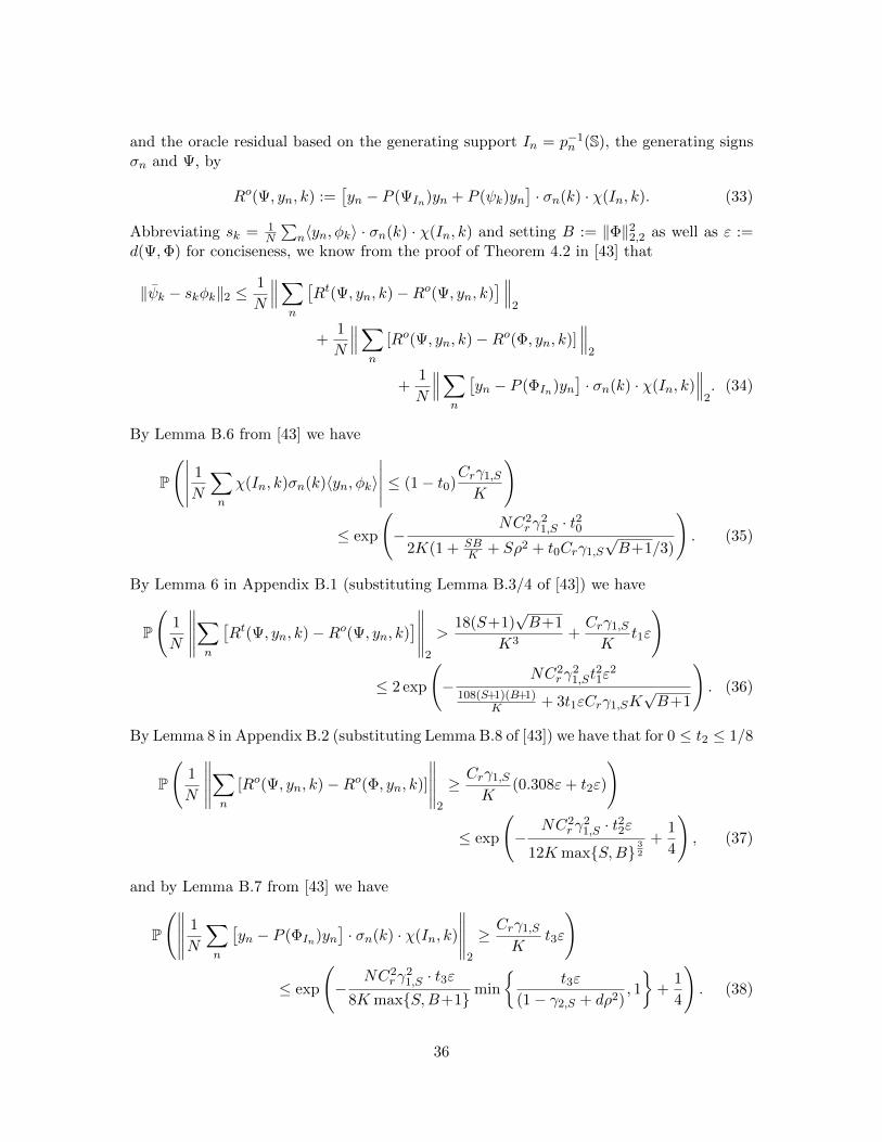
and the oracle residual based on the generating support In = p−1n (S), the generating signs

σn and Ψ, by

Ro(Ψ, yn, k) :=[yn − P (ΨIn)yn + P (ψk)yn

]· σn(k) · χ(In, k). (33)

Abbreviating sk = 1N

∑n〈yn, φk〉 · σn(k) · χ(In, k) and setting B := ‖Φ‖22,2 as well as ε :=

d(Ψ,Φ) for conciseness, we know from the proof of Theorem 4.2 in [43] that

‖ψk − skφk‖2 ≤1

N

∥∥∥∑n

[Rt(Ψ, yn, k)−Ro(Ψ, yn, k)

] ∥∥∥2

+1

N

∥∥∥∑n

[Ro(Ψ, yn, k)−Ro(Φ, yn, k)]∥∥∥

2

+1

N

∥∥∥∑n

[yn − P (ΦIn)yn

]· σn(k) · χ(In, k)

∥∥∥2. (34)

By Lemma B.6 from [43] we have

P

(∣∣∣∣∣ 1

N

∑n

χ(In, k)σn(k)〈yn, φk〉

∣∣∣∣∣ ≤ (1− t0)Crγ1,S

K

)

≤ exp

(−

NC2rγ

21,S · t20

2K(1 + SBK + Sρ2 + t0Crγ1,S

√B+1/3)

). (35)

By Lemma 6 in Appendix B.1 (substituting Lemma B.3/4 of [43]) we have

P

(1

N

∥∥∥∥∥∑n


]∥∥∥∥∥2

>18(S+1)

√B+1

K3+Crγ1,S

Kt1ε

)

≤ 2 exp

(−

NC2rγ

21,St

21ε

2

108(S+1)(B+1)K + 3t1εCrγ1,SK

√B+1

). (36)

By Lemma 8 in Appendix B.2 (substituting Lemma B.8 of [43]) we have that for 0 ≤ t2 ≤ 1/8

P

(1

N

∥∥∥∥∥∑n

[Ro(Ψ, yn, k)−Ro(Φ, yn, k)]

∥∥∥∥∥2

≥Crγ1,S

K(0.308ε+ t2ε)

)

≤ exp

(−

NC2rγ

21,S · t22ε

12K maxS,B32

+1

4

), (37)

and by Lemma B.7 from [43] we have

P

(∥∥∥∥∥ 1

N

∑n

[yn − P (ΦIn)yn

]· σn(k) · χ(In, k)

∥∥∥∥∥2

≥Crγ1,S

Kt3ε

)

≤ exp

(−

NC2rγ

21,S · t3ε

8K maxS,B+1min

t3ε

(1− γ2,S + dρ2), 1

+

1

4

). (38)

36

Thus, with high probability we have sk ≥ (1− t0)Crγ1,S

K and

∥∥ψk − skφk∥∥2≤Crγ1,S

K

(18(S+1)

√B+1

K2Crγ1,Sε+ t1 + 0.308 + t2 + t3

)ε. (39)

Note that we only need to take into account distances ε > 132√S

, so we will use some crude

bounds on Crγ1,S to show that the fraction with ε in the denominator above is small. Therequirement that ‖c(Sc)‖2/c(1) ≤ γapp ≤ 12

7

√logK ensures that γ1,S ≥ (1 + 3 logK)−1/2

and we trivially have γ1,S ≥ Sc(S). Combining this with the bound on Cr in (10) we get

1

Crγ1,S≤

√1 + 5dρ2

(1− e−d)γ1,S≤√

1 + 3 logK

(1− e−d)+

ρ

c(S)

√5d

S(1− e−d). (40)

The conditions in (31) imply that K ≥ 142SB logK, which in turn means that logK > 7,as well as ρ/c(S) ≤ γρ ≤ 1/(40

√logK). Assuming additionally that K ≥

√d, meaning the

dictionary is not too undercomplete, this leads to

18(S+1)√B+1

K2Crγ1,Sε≤ 0.025, (41)

for B ≥ 1 and S ≥ 2. Setting t0 = t1 = 1/20 and t2 = t3 = 1/8 we get

maxk

∥∥ψk − skφk∥∥2≤ 0.633 ·

Crγ1,S

Kε and min

ksk ≥ 0.95 ·

Crγ1,S

K, (42)

which by Lemma B.10 from [43] implies that

d(Ψ,Φ)2 = maxk

∥∥∥∥ ψk‖ψk‖2

− φk∥∥∥∥2

2

≤ 2

(1−

√1− 0.6332ε2

0.952

)≤ 2 · 0.6332ε2

0.952≤ 0.89ε2, (43)

except with probability

K exp

(−

NC2rγ

21,S

K(801 + 14Crγ1,S

√B+1)

)+ 2K exp

(−

NC2rγ

21,S · ε2

K( 110 + 60εCrγ1,S

√B+1)

)

+ e14K exp

(−

NC2rγ

21,S · ε

768K maxS,B32

)+ e

14K exp

(−

NC2rγ

21,S · ε2

512K maxS,B+1 (1 + dρ2)

).

The final probability bound follows from the observations that Crγ1,S ≤√S, B+1 ≥ 2 and

ε ≤√

2.

Appendix B. Technical Lemmata

Here we state the proofs of the two lemmata characterising the difference between thethresholding and the oracle residual resp. the difference between the oracle residuals basedon the generating dictionary and a perturbation.

37

B.1 Difference between thresholding and oracle residual

To prove Lemma 6 we will make use of the scalar version of Bernstein’s inequality [7] andHoeffding’s inequality [20]. We will also need Proposition 5, which is based on a version ofFreedman’s inequality, [16], to deal with sums of dependent random variables.

Theorem 3 (Scalar Bernstein, [7]) Let vn ∈ R, n = 1 . . . N , be a finite sequence ofindependent random variables with zero mean. If E(v2

n) ≤ m and E(|vn|k) ≤ 12k!mMk−2

for all k > 2, then for all t > 0 we have

P

(∑n

vn ≥ t

)≤ exp

(− t2

2(Nm+Mt)

).

To prove Proposition 5 we need the following simplified version of Freedman’s inequality.

Theorem 4 (Freedman, [16]) Let X0, . . . , XS be a martingale sequence with bounded dif-ferences, that is |Xk − Xk−1| ≤ c almost surely for each k. Moreover, let the predictable

quadratic variation 〈X〉S =∑S

k=1 E[(Xk −Xk−1)2

∣∣∣Fk−1

]be bounded by b. Then for all

t > 0

P (XS −X0 ≥ t) ≤ exp

(− t2

2(ct+ b)

).

Proposition 5 Let v ∈ RK be a vector, I = (i1, . . . , iS) be a sequence of length S ob-tained by sampling from K = 1, . . . ,K without replacement, ε with values in −1, 1S aRademacher vector independent from I and c ∈ RS a scaling vector. Then for any t ≥ 0,

P

(|S∑k=1

ckεkvik | ≥ t

)≤ 2 exp

(−t2

2(‖c‖∞‖v‖∞t+ ‖c‖22 · ‖v‖22/(K − S))

). (44)

Proof We will use Theorem 4 on an appropriately constructed martingale. Let I =(i1, . . . , iS), be the random vector obtained by sampling from K = 1, . . . ,K withoutreplacement, that is, I is drawn uniformly at random from the set

Ω := ω ∈ KS : ωi 6= ωj for i 6= j.

We equip Ω with the σ-algebra F := P(Ω) and the point measure P(ω) := |Ω|−1, to getthe probability space (Ω,F ,P). We also set ∆ := −1, 1S , equip it with the σ-algebra A :=P(∆), the point measure Q(δ) = 2−S and define the product space (Ω×∆,F⊗A,P⊗Q).On Ω we define the filtration ∅,Ω = F0 ⊆ F1 ⊆ · · · ⊆ FS = F , where Fk is the σ-algebrainduced by ω1, . . . , ωk. To be exact, we define the random variables

ij : Ω −→K ⊆ R with ij(ω) := ωj ,

and set Fk := σ(i1, . . . , ik) for all 1 ≤ k ≤ S.Since we also want to condition on the signs δ ∈ ∆, we define the random variables

εj : ∆ −→−1, 1 ⊆ R with εj(δ) := δj ,

38

and the corresponding filtration ∅,∆ = A0 ⊆ A1 ⊆ · · · ⊆ AS = A, by setting Ak =σ(ε1, . . . , εk). On the product space Ω×∆ we then get the filtration Fk ⊗Ak.Next we define the bounded random variables

Xk : Ω×∆ −→ R, with Xk(ω, δ) =

k∑j=1

cjεj(δ)vij(ω).

The random variables Xk form a martingale sequence with resp. to the filtration Fk ⊗Ak,since by independence of εk to F ⊗Ak−1 we have

E[Xk −Xk−1|Fk−1 ⊗Ak−1] = E[E[ckεkvik |F ⊗ Ak−1]

∣∣Fk−1 ⊗Ak−1

]= ckE [vikE[εk|F ⊗ Ak−1]|Fk−1 ⊗Ak−1] = 0.

The sum we want to estimate is XS with expectation E(XS) = 0 = X0. Further we have|Xk−Xk−1| = |ckεkvik | ≤ ‖c‖∞‖v‖∞ as well as (Xk−Xk−1)2 = c2

kv2ik

, so we can bound thepredictable quadratic variation as

〈X〉S =

S∑k=1

E[(Xk −Xk−1)2

∣∣Fk−1 ⊗Ak−1

]=

S∑k=1

E[c2kv

2ik

∣∣Fk−1 ⊗Ak−1

]=

S∑k=1

c2k

∑`/∈i1,...,ik−1

v2`

1

K − k + 1≤ ‖c‖22

‖v‖22K − S

The final result follows using the symmetry of XS .

Now we are ready to prove the lemma estimating the error originating from thresholdingfailing to recover the generating supports and signs.

Lemma 6 Assume that the signals yn follow model (7) for coefficients with gap c(S+1)/c(S) ≤ γgap, dynamic sparse range c(1)/c(S) ≤ γdyn, noise to coefficient ratio ρ/c(S) ≤γρ and relative approximation error ‖c(Sc)‖2/c(1) ≤ γapp ≤ 12

7

√logK. If the cross Gram

matrix Φ?Ψ is diagonally dominant in the sense that

mink|〈ψk, φk〉| ≥max

8 γgap ·max

k|〈ψk, φk〉| ,

40 γρ ·√

logK,

48 γdyn · logK · µ(Φ,Ψ),

14 γdyn ·√‖Φ‖22,2S logK/(K−S)

, (45)

then

P

1

N

∥∥∥∥∥∑n


]∥∥∥∥∥2

>18(S+1)

√‖Φ‖22,2+1

K3+Crγ1,S

Ktε

≤ 2 exp

− NC2rγ

21,St

2ε2

108(S+1)(‖Φ‖22,2+1)

K + 3tεCrγ1,SK√‖Φ‖22,2+1

. (46)

39

Proof Throughout the proof we will use the abbreviations B = ‖Φ‖22,2 and µ = µ(Φ,Ψ).To estimate the difference between the oracle and the thresholding residuals, we have todistinguish between four different cases, based on whether k is in the oracle support or notand whether thresholding recovers the oracle support and sign, so we set

F = n : k ∈ In ∧(Itn 6= In ∨ sign(〈ψk, yn〉) 6= σn(k)

),

G = n : k /∈ In ∧ k ∈ Itn.

Whenever a signal is not in one of the sets above, the residuals coincide, yielding

∆ =∥∥∥∑

n


] ∥∥∥2

=∥∥∥ ∑n∈F∪G


] ∥∥∥2. (47)

Further observing that operators of the form Id−P (ΨJ)+P (ψk) with k ∈ J are orthogonalprojections, and that our signals are bounded, ‖yn‖2 ≤

√B + 1, as well as Ro(Ψ, yn, k) = 0

for n ∈ G leads to

∆ ≤∑

n∈F∪G

(‖Rt(Ψ, yn, k)‖2 + ‖Ro(Ψ, yn, k)‖

)≤ (2|F|+ |G|)

√B + 1. (48)

To upper bound the size of the set F , we apply Bernstein’s inequality to the sum of Ni.i.d copies of the centered random variable 1F − P(F ), where

F =y : k ∈ I ∧

(It 6= I ∨ sign(〈ψk, y〉) 6= σ(k)

), (49)

which leads to

P(|F| ≥ NP(F ) +Nt) ≤ exp

(− t2N

2P(F ) + t

). (50)

Similarly defining G = y : k /∈ I ∧ k ∈ It, we get

P(|G| ≥ NP(G) +Nt) ≤ exp

(− t2N

2P(G) + t

). (51)

So what remains to calculate is the probability of the events F and G, that is of thresholdingfailing to recover the oracle support and sign when k is in the support and of accidentallyrecovering k when it is not in the support.

Step 1 - Failure probability of the recovery of I or the correct sign σ(k)

Here we will show that with high probability for a signal y following the model in (7) withk ∈ I, we have It = I = p−1(S) and sign(〈ψk, y〉) = σ(k).To ensure It = I, this means the recovery of all i ∈ I, we need to have

mini∈I|〈ψi, y〉| > max

i/∈I|〈ψi, y〉|. (52)

40

Expanding the inner product of a rescaled signal y with an atom ψi of the perturbeddictionary Ψ yields

|〈ψi,Φxc,p,σ + r〉| = |∑j

σ(j)c(p(j))〈ψi, φj〉+ 〈ψi, r〉|

= |c(p(i))〈ψi, φi〉+ σ(i)∑j 6=i

σ(j)c(p(j))〈ψi, φj〉+ σ(i)〈ψi, r〉|.

Depending on the index i under consideration, we obtain the following bounds from belowresp. above (remember that αmin ≤ |〈ψi, φi〉| ≤ αmax),

i ∈ I : |〈ψi,Φxc,p,σ + r〉| ≥ c(S)αmin −∣∣∑j 6=i

σ(j)c(p(j))〈ψi, φj〉∣∣− |〈ψi, r〉|,

i /∈ I : |〈ψi,Φxc,p,σ + r〉| ≤ c(S + 1)αmax +∣∣∑j 6=i

σ(j)c(p(j))〈ψi, φj〉∣∣+ |〈ψi, r〉|.

This means that a sufficient condition for the recovery of I is that for all i

∣∣∑j 6=i

σ(j)c(p(j))〈ψi, φj〉∣∣ < θ1 · c(S)αmin and |〈ψi, r〉| < θ2 · c(S)αmin, (53)

where θ1 and θ2 ensure that

c(S)αmin−θ1c(S)αmin − θ2c(S)αmin

!≥ c(S + 1)αmax + θ1c(S)αmin + θ2c(S)αmin. (54)

Since the conditions above also guarantee the recovery of the correct sign σ(i) for all i ∈I, so in particular the recovery of σ(k), we can bound the probability of the event thatthresholding fails while k is in the generating support I as

P([It 6= I ∨ sign(〈ψk, y〉) 6= σ(k)

]∧ k ∈ I

)≤∑i

P(∣∣∑

j 6=iσ(j)c(p(j))〈ψi, φj〉

∣∣ ≥ θ1c(S)αmin ∧ k ∈ I)

+∑i

P(|〈ψi, r〉| ≥ θ2c(S)αmin ∧ k ∈ I

)≤∑i

∑`∈S

P(∣∣∑


∣∣ ≥ θ1c(S)αmin

∣∣p(k) = `)· P(p(k) = `)

+∑i

∑`∈S

P(|〈ψi, r〉| ≥ θ2c(S)αmin

∣∣p(k) = `)· P(p(k) = `).

Since every permutation is equally likely, each index is equally likely to be mapped to `,meaning P(p(k) = `) = 1/K. Using the independence of the noise from the remaining signal

41

parameters and its sub-Gaussian property further leads to

P([It 6= I ∨ sign(〈ψk, y〉) 6= σ(k)

]∧ k ∈ I

)≤ 1

K

∑i

∑`∈S

P(∣∣∑



∣∣p(k) = `)

+S

K

∑i

P(|〈ψi, r〉| ≥ θ2c(S)αmin

)≤ 1

K

∑i

∑`∈S

P(∣∣∑



∣∣p(k) = `)

+ 2S exp

(−(θ2c(S)αmin)2

2ρ2

). (55)

To estimate the terms P(∣∣∑

j 6=i σ(j)c(p(j))〈ψi, φj〉∣∣ ≥ θ1c(S)αmin

∣∣p(k) = `), we split the

sum into two parts; one over j ∈ I \ i, k, that captures most of the energy, and the otherover j ∈ (Ic ∪ k) \ i. For m1 ∈ (0, 1) and m2 = 1−m1 we have

P(∣∣∑



∣∣p(k) = `)

≤ P(∣∣ ∑

j∈I\i,k

σ(j)c(p(j))〈ψi, φj〉∣∣ ≥ m1θ1c(S)αmin

∣∣p(k) = `)

+ P(∣∣ ∑

j∈(Ic∪k)\i

σ(j)c(p(j))〈ψi, φj〉∣∣ ≥ m2θ1c(S)αmin

∣∣p(k) = `).

The first term we estimate using Proposition 5 and the second term using Hoeffding’sinequality. With some small simplifications we get for all i, including k,

P(∣∣∑



∣∣p(k) = `)

≤ 2 exp

(−(m1θ1c(S)αmin)2

2(c(1)µ ·m1θ1c(S)αmin + ‖c(S)‖22 BK−S )

)+ 2 exp


2µ2(c(`)2 + ‖c(Sc)‖22)

)≤ 2 exp

(−1

4min

c(S)m1θ1αmin

c(1)µ,(K − S)(m1θ1c(S)αmin)2

B‖c(S)‖22

)+ 2 exp

(−1

4min

(c(S)m2θ1αmin)2

c(1)2µ2,(c(S)m2θ1αmin)2

µ2‖c(Sc)‖22

).

Substituting the expression above into (55) we get

P([It 6= I ∨ sign(〈ψk, y〉) 6= σ(k)

]∧ k ∈ I

)≤ 2S exp

(−1

4min

c(S)m1θ1αmin


B‖c(S)‖22

)+ 2S exp

(−1

4min

(c(S)m2θ1αmin)2

c(1)2µ2,(c(S)m2θ1αmin)2

µ2‖c(Sc)‖22

)+ 2S exp

(−(θ2c(S)αmin)2

2ρ2

),

42

where θ1 and θ2 have to ensure (54) and m1 +m2 = 1. From this, whenever

αmin ≥ max

1

1− 2θ1 − 2θ2

c(S + 1)

c(S)αmax,

4n

m1θ1

c(1)

c(S)µ logK,

2√n

m1θ1

‖c(S)‖2c(S)

√B logK

K − S,

2√n

(1−m1)θ1

c(1)

c(S)µ√

logK,2√n

(1−m1)θ1

‖c(Sc)‖2c(S)

µ√

logK,

√2n

θ2

ρ

c(S)

√logK

,

we get that

P([It 6= I ∨ sign(〈ψk, y〉) 6= σ(k)

]∧ k ∈ I

)≤ 6S ·K−n.

Setting θ1 = 616 , θ2 = 1

16 , m1 = 23 , n = 3, the probability that thresholding fails to recover

I and/or the corresponding signs, restricted to the signals for which we have k ∈ I, isbounded by 6S ·K−3, whenever

αmin ≥ max

8c(S + 1)

c(S)αmax, 48

c(1)

c(S)µ logK, 14

c(1)

c(S)

√SB logK

K − S, 40

ρ

c(S)

√logK

,

and ‖c(Sc)‖2

c(1) ≤ 127

√logK, where we have used that ‖c(S)‖2 ≤

√Sc(1).

Step 2 - Probability of wrongly recovering k for k /∈ I - P(k ∈ It|k /∈ I)

As a second step we will bound the probability of wrongly recovering an atom ψk when itis not in the generating support, meaning k /∈ I. A sufficient condition for not recovering kis that

mini∈I|〈ψi, y〉| > |〈ψk, y〉|. (56)

Using the bounds from step 1,

i ∈ I : |〈ψi,Φxc,p,σ + r〉| ≥ c(S)αmin −∣∣∑j 6=i

σ(j)c(p(j))〈ψi, φj〉∣∣− |〈ψi, r〉|,

k /∈ I : |〈ψk,Φxc,p,σ + r〉| ≤ c(S + 1)αk +∣∣∑j 6=k

σ(j)c(p(j))〈ψk, φj〉∣∣+ |〈ψk, r〉|,

we get as sufficient condition for not recovering k, that for all i ∈ I ∪ k∣∣∑j 6=i

σ(j)c(p(j))〈ψi, φj〉∣∣ < θ1 · c(S)αmin and |〈ψi, r〉| < θ2 · c(S)αmin,

where θ1 and θ2 again ensure that

c(S)αmin − θ1c(S)αmin − θ2c(S)αmin

!≥ c(S + 1)αk + θ1c(S)αmin + θ2c(S)αmin.

43

We now bound the probability of thresholding recovering k when it is not in the gener-ating support I as

P(k ∈ It ∧ k /∈ I) =∑`>S

P(k ∈ It∣∣p(k) = `) · P(p(k) = `)

≤ 1

K

∑`>S

∑i∈I∪k

P(∣∣∑


∣∣ ≥ θ1 · c(S)αmin

∣∣p(k) = `)

+1

K

∑`>S

∑i∈I∪k

P(|〈ψi, r〉| ≥ θ2 · c(S)αmin

∣∣p(k) = `).

Using the same splitting technique as in step 1, and the sub-Gaussian property of r, we get

P(k ∈ It ∧ k /∈ I) ≤ 2(S + 1) exp

(−1

4min

c(S)m1θ1αmin


B‖c(S)‖22

)+ 2(S + 1) exp


2µ2‖c(Sc)‖22

)+ 2(S + 1) exp

(−(θ2c(S)αmin)2

2ρ2

).

To have this probability sufficiently small, we need to have

αmin ≥ max

1

1− 2θ1 − 2θ2

c(S + 1)

c(S)αk,

4n

m1θ1

c(1)

c(S)µ logK,

2√n

m1θ1

‖c(S)‖2c(S)

√B logK

K − S,

√2n

(1−m1)θ1

‖c(Sc)‖2c(S)

µ√

logK,

√2n

θ2

ρ

c(S)

√logK

.

Choosing the same values as before, θ1 = 616 , θ2 = 1

16 , m1 = 23 , n = 3, we arrive at the

bound

P(k ∈ It ∧ k /∈ I) ≤ 6(S + 1) ·K−3,

whenever ‖c(Sc)‖2

c(1) ≤ 125

√logK and

αmin ≥ max

8c(S + 1)

c(S)αk, 48

c(1)

c(S)µ logK, 14

c(1)

c(S)

√SB logK

K − S, 40

ρ

c(S)

√logK

.

Using all these estimates, we are now ready to bound the error originating from the differencebetween the thresholding and the oracle residual.

Step 3 - Putting it all together

Using all previous estimates, what remains to do is to estimate the size of F and G andfinally put all pieces together. Inserting our probability estimates into (50) and (51), weget

P(|F| ≥ N

(6S

K3+

Crγ1,S

3K√B + 1

tε

))≤ exp

(−

NC2rγ

21,St

2ε2

108S(B+1)K + 3tεCrγ1,SK

√B + 1

)

44

and

P(|G| ≥ N

(6(S + 1)

K3+

Crγ1,S

3K√B + 1

tε

))≤ exp

(−

NC2rγ

21,St

2ε2

108(S+1)(B+1)K + 3tεCrγ1,SK

√B + 1

),

respectively. As we have∥∥∥∑n


] ∥∥∥2≤ (2|F|+ |G|)

√B + 1,

in summary, we get

P

(1

N

∥∥∥∑n


] ∥∥∥2>

18(S + 1)√B + 1

K3+Crγ1,S

Ktε

)

≤ 2 exp

(−

NC2rγ

21,St

2ε2

108(S+1)(B+1)K + 3tεCrγ1,SK

√B + 1

).

Next we will prove the lemma yielding a bound for the error originating from the differencebetween the oracle residuals based on the generating dictionary and a perturbation of it.

B.2 Difference between oracle residuals

For the proof of Lemma 8 we will use the vector version of Bernstein’s inequality.

Theorem 7 (Vector Bernstein, [24, 19, 25]) Let (vn)n ∈ Rd be a finite sequence of in-dependent random vectors. If ‖vn‖2 ≤M almost surely, ‖E(vn)‖2 ≤ m1 and

∑n E(‖vn‖22) ≤

m2, then for all 0 ≤ t ≤ m2/(M +m1), we have

P

(∥∥∥∥∥∑n

vn −∑n

E(vn)

∥∥∥∥∥2

≥ t

)≤ exp

(− t2

8m2+

1

4

), (57)

and, in general,

P

(∥∥∥∥∥∑n

vn −∑n

E(vn)

∥∥∥∥∥2

≥ t

)≤ exp

(− t

8·min

t

m2,

1

M +m1

+

1

4

). (58)

Note that the general statement is simply a consequence of the first part, since for t ≥m2/(M +m1) we can choose m2 = t(M +m1).

We next prove that, assuming incoherence and good conditioning of the perturbed dictio-nary, the oracle residuals based on the perturbed dictionary Ψ and the generating dictionaryΦ are close to each other.

45

Lemma 8 Assume that the signals yn follow the random model in (7). Further, assume

that S ≤ min

K98‖Φ‖22,2

, 198ρ2

and that the current estimate of the dictionary Ψ has distance

d(Φ,Ψ) = ε ≥ 132√S

but is incoherent and well conditioned, meaning its coherence µ(Ψ) and

its operator norm ‖Ψ‖2,2 satisfy

µ(Ψ) ≤ 1


K

134e2S logK− 1. (59)

Then for all 0 ≤ t ≤ 1/8 we have

P

(1

N

∥∥∥∥∥∑n


∥∥∥∥∥2

≥Crγ1,S

K(0.308ε+ tε)

)

≤ exp

(−

NC2rγ

21,St

2ε

12K maxS, ‖Φ‖22,232

+1

4

).

Proof Throughout the proof we will use the abbreviations B = ‖Φ‖22,2 and B = ‖Ψ‖22,2. Weapply Theorem 7 to vn = Ro(Ψ, yn, k)−Ro(Φ, yn, k) and drop the index n for conciseness.From Lemma B.8 in [43] we know that v = T (I, k)y · σ(k) · χ(I, k), where T (I, k) :=P (ΦI)− P (ΨI)− P (φk) + P (ψk), and that

E(v) =Crγ1,S

K

(K−1

S−1

)−1 ∑|I|=S,k∈I

[P (ψk)− P (ΨI)

]φk. (60)

Using the orthogonal decomposition φk = [P (ψk) + Q(ψk)]φk, where P (ψk)Q(ψk) = 0, weget

E(v) =Crγ1,S

K

(K−1

S−1

)−1 ∑|I|=S,k∈I

−P (ΨI)Q(ψk)φk. (61)

Since the perturbed dictionary Ψ is well-conditioned and incoherent, for most I the sub-dictionary ΨI will be a quasi isometry and P (ΨI) ≈ ΨIΨ

?I . We therefore expand the

expectation above, using the abbreviation pK,S =(K−1S−1

)−1, as

K

Crγ1,SE(v) = pK,S

∑|I|=S,k∈I

[ΨIΨ

?I − P (ΨI)]Q(ψk)φk −

∑|I|=S,k∈I

ΨI\kΨ?I\kQ(ψk)φk

= pK,S

∑|I|=S,k∈I

[ΨIΨ


(K−2

S−2

)∑j 6=k

ψjψ?jQ(ψk)φk

= pK,S

∑|I|=S,k∈I

[ΨIΨ


S−1

K−1(ΨΨ? − ψkψ?k)Q(ψk)φk

= pK,S∑

|I|=S,k∈Iδ(ΨI )≤δ0

[ΨIΨ

?I − P (ΨI)]Q(ψk)φk

+ pK,S∑

|I|=S,k∈Iδ(ΨI )>δ0

[ΨIΨ


S−1

K−1ΨΨ?Q(ψk)φk.

46

Since for ψk = αkφk + ωkzk we have ‖Q(ψk)φk‖2 = ωk ≤ ε, we can bound the norm of theexpectation above as

‖E(v)‖2 ≤Crγ1,S

K

[δ0 + P

(δ(ΨI) > δ0

∣∣|I| = S, k ∈ I)· (B+1) +

(S−1)B

K−1

]ε. (62)

To estimate the probability of a subdictionary being ill-conditioned we use Chretien andDarses’s results on the conditioning of random subdictionaries, which are slightly cleanerand thus easier to handle than the original results by Tropp, [50]. Theorem 3.1 of [10]reformulated for our purposes and applied to Ψ states that

P(δ(ΨI) > δ0

∣∣|I| = S)≤ 216K exp

(−min

δ0

2µ(Ψ),δ2

0K

4e2SB

). (63)

Together with the union bound,

P(δ(ΨI) > δ0

∣∣|I| = S, k ∈ I)≤ K

S· P(δ(ΨI) > δ0

∣∣|I| = S), (64)

this leads to

‖E(v)‖2 ≤Crγ1,S

K

[δ0 +

216K2(B+1)

Sexp

(−min

δ0

2µ(Ψ),δ2

0K

4e2SB

)+SB

K

]ε. (65)

Choosing δ0 = 3/10, as long as B ≤ K134e2S logK

− 1 and µ(Ψ) ≤ 120 logK we have

‖E(v)‖2 ≤ 0.308 ·Crγ1,S

K· ε, (66)

where we used that S ≥ 2 and logK ≥ 7. The second quantity we need to bound is theexpected energy of v = T (I, k)y ·σ(k) ·χ(I, k). Combining Eqs. (115-118) from Lemma B.8in [43] we get that

E(‖v‖22) ≤ Ep(χ(I, k)

[4γ2,Sε

2 +

(B(1− γ2,S)

K−S+ ρ2

)‖T (I, k)‖2F

]). (67)

Since we are only interested in the regime ε > O(1/√S) we will accept an additional factor

S in the final sample complexity in return for a crude but painless estimate. Concretely, weuse that T (I, k) is the difference of two orthogonal projections onto subspaces of dimensionS−1, namely P (ΦI) − P (φk) and P (ΨI) − P (ψk). This leads to the bound ‖T (I, k)‖2F ≤2(S−1) ≤ 2S and we get

E(‖v‖22) ≤ S

K

(4γ2,Sε

2 +2BS

K−S(1− γ2,S) + 2Sρ2

)≤ S

K(4ε2 + 1/24), (68)

where for the second inequality we have used the assumption S ≤ min K98B ,

198ρ2 .

Combining the estimates for ‖E(v)‖2 and E(‖v‖22) with the norm bound ‖v‖2 ≤ 2√B+1,

47

we get that for ε ≥ 132√S

and 0 ≤ t ≤ 1/8

P

(1

N

∥∥∥∥∥∑n


∥∥∥∥∥2

≥Crγ1,S

K(0.308ε+ tε)

)

≤ exp

(−NCrγ1,Stε

8Kmin

Crγ1,Stε

S(4ε2 + 1/24),

1

ε+ 2√B+1

+

1

4

)≤ exp

(−NC2

rγ21,St

2ε

8Kmin

1

S(4ε+ (24ε)−1),

1

3tγ1,S

√B+1

+

1

4

)

≤ exp

(−

NC2rγ

21,St

2ε

8K maxS,Bmin

1

4ε+ (24ε)−1,

1

3t√

2

+

1

4

)

≤ exp

(−

NC2rγ

21,St

2ε

12K maxS,B32

+1

4

).

48

Appendix C. Pseudocode

Algorithm C.1: ITKrM augmented for replacement/adaptivity - one iteration

a/r Input: Ψ, Y, S,Γ,M ; // dictionary, signals, sparsity, candidates,

// minimal observations (only for adaptive)

Set: m = blog de, NΓ = bN/mc;Initialise: Ψ = 0, Γ = 0, S = 0;

foreach n do

// basic ITKrM steps

Itn = arg maxI:|I|=S ‖Ψ?Iyn‖1 ; // thresholding

xn = Ψ†Itnyn ; // sparse coefficients

an = yn −ΨItnxn ; // residual

r τ = 0 ; // simple counter for replacement

a τ =(2 log

(2NM

)‖an‖22 + ‖ΨItn

xn‖22)/d ; // advanced counter for adaptivity

foreach k ∈ Itn doψk ← ψk +

[an + P (ψk)yn

]· sign(〈ψk, yn〉) ; // atom update

if |xn(k)|2 ≥ τ thenv(k)← v(k) + 1 ; // atom value update

end

end

// steps for replacement candidates

in = arg max` |〈γ`, an〉| ; // residual thresholding

γin ← γin + an · sign(〈γin , an〉) ; // candidate update

r τΓ = 2 log(2K)/d ; // simple counter for replacement

a τΓ = 2 log( 2NΓ

d )/d ; // advanced counter for adaptivity

if |〈γin , an〉|2 ≥ τΓ ‖an‖22 thenvΓ(in)← vΓ(in) + 1 ; // candidate value update

end

if n (mod NΓ) == 0 ∧ n < mNΓ thenΓ← (γ1/‖γ1‖2, . . . , γL/‖γL‖2) ; // candidate normalisation

Γ = 0 ; // cand. iteration restart

a vΓ = 0 ; // skip for replacement

end

a // steps for estimating sparsity level, skip for replacement

a θ =(2 log(4K)‖an‖22 + ‖ΨItn

xn‖22)/d;

a S ← S + ]k : |xn(k)|2 ≥ θ ; // correct atoms

a S ← S + ]k : |〈ψk, an〉|2 ≥ θ ; // missed atoms

end

Ψ←(ψ1/‖ψ1‖2, . . . , ψK/‖ψK‖2

); // atom normalisation

a S ← bS/Ne ; // average sparsity level, skip for replacement

a/r Output: Ψ, v,Γ, vΓ, S; // estimated sparsity only for adaptivity

49

Algorithm C.2: Replacing coherent atoms (delete, merge, add)

Input: Ψ, v,Γ, vΓ, µmax; // dict., score, cand., cand.score, threshold

Reorder Γ, vΓ s.t. vΓ(1) ≥ vΓ(2) ≥ . . . ≥ vΓ(L);Find: (k, k′) = arg maxi<j |〈ψi, ψj〉|; // most coherent atom pair

while |〈ψk, ψk′〉| > µmax ∧ Γ 6= [] doh = sign(〈ψk, ψk′〉);

d ψk = b v(k′)v(k′)+v(k)eψk′ + hb v(k)

v(k′)+v(k)eψk ; // delete

m ψk = v(k′)ψk′ + hv(k)ψk ; // or merge

a ψk = ψk′ + hψk′ ; // or add

ψk ← ψk/‖ψk‖2;Find Λ = ` : µ` := maxi6=k,k′ |〈γ`, ψi〉| > |〈ψk, ψk′〉|;ΓΛ ← [], vΓ(Λ)← []; // discard coherent candidates

if Γ 6= [] thenψk ← ψk; // replace with merged atom

v(k)← v(k) + v(k′) ; // update score of merged atom

ψk′ ← γ1; // replace with most useful candidate

if µ1 < µmax thenv(k′) = vΓ(1); // update with candidate score

elsev(k′) = 0; // preferably replaced again

endγ1 ← [], vΓ(1)← []; // discard used candidate

endFind: (k, k′) = arg maxi<j |〈ψi, ψj〉| ; // update most coherent atom pair

end

Output: Ψ, v,Γ, vΓ

Algorithm C.3: Pruning coherent atoms (merge)

Input: Ψ, V = (v1, . . . , vK), µmax; // dictionary, last m scores, threshold

∆ = ∅ ; // initialise set of atoms to delete

H = Ψ?Ψ− IK ; // hollow Gram matrix in absolute

Find: (k, k′) = arg maxi<j |H(i, j)|; // most coherent atom pair

while |H(k, k′)| > µmax do

m ψk ← vk′(1)ψk′ + sign(〈ψk, ψk′〉)vk(1)ψk ; // merge according to most recent score

ψk ← ψk/‖ψk‖2;vk(1)← vk′(1) + vk(1) ; // update most recent score

∆← ∆ ∪ k′;H(k, ·)← 0, H(k′, ·)← 0, H(·, k)← 0, H(·, k′)← 0 ; // update hollow Gram matrix

Find: (k, k′) = arg maxj<i |H(i, j)| ; // update most coherent atom pair

endΨ∆ ← [], V∆ ← []; // delete atoms

Output: Ψ, V

50

Algorithm C.4: Pruning unused atoms

Input: Ψ, V = (v1, . . . , vK),M, δ; // dictionary, last m scores, threshold,

// maximally pruned atoms

foreach k dov(k) = maxi vk(i) ; // maximum of last m scores

end∆ = k : v(k) < M ; // atoms with max.scores below threshold

if |∆| > δ thenSort: v(i1) ≤ v(i2) ≤ · · · ≤ v(iK) ; // sort max.score

∆ = i1 . . . iδ) ; // δ atoms with smallest max.scores

endΨ∆ ← [], V∆ ← []; // delete atoms

Output: Ψ, V

Algorithm C.5: Adding atoms

Input: Ψ, V,Γ, vΓ, µmax,M

Sort: vΓ(i1) ≥ vΓ(i2) ≥ . . . ≥ vΓ(iL); // sort according to score

L = |` : vΓ(`) ≥ d|; // score above d

for ` = 1 . . . L doif maxk |〈ψk, γi`〉| ≤ µmax then

Ψ← (Ψ, γi`) ; // in order of score add if incoherent

V ← (V,M · 1); // set last m scores of added atoms to M

end

end

Output: Ψ, V

References

[1] A. Agarwal, A. Anandkumar, P. Jain, P. Netrapalli, and R. Tandon. Learningsparsely used overcomplete dictionaries via alternating minimization. In COLT 2014(arXiv:1310.7991), 2014.

[2] A. Agarwal, A. Anandkumar, and P. Netrapalli. Exact recovery of sparsely used over-complete dictionaries. In COLT 2014 (arXiv:1309.1952), 2014.

[3] M. Aharon, M. Elad, and A.M. Bruckstein. K-SVD: An algorithm for designing over-complete dictionaries for sparse representation. IEEE Transactions on Signal Process-ing., 54(11):4311–4322, November 2006.

[4] S. Arora, R. Ge, and A. Moitra. New algorithms for learning incoherent and overcom-plete dictionaries. In COLT 2014 (arXiv:1308.6273), 2014.

[5] S. Arora, R. Ge, T. Ma, and A. Moitra. Simple, efficient, and neural algorithms forsparse coding. In COLT 2015 (arXiv:1503.00778), 2015.

51

[6] B. Barak, J.A. Kelner, and D. Steurer. Dictionary learning and tensor decompositionvia the sum-of-squares method. In STOC 2015 (arXiv:1407.1543), 2015.

[7] G. Bennett. Probability inequalities for the sum of independent random variables.Journal of the American Statistical Association, 57(297):33–45, March 1962.

[8] E. Candes, J. Romberg, and T. Tao. Robust uncertainty principles: exact signalreconstruction from highly incomplete frequency information. IEEE Transactions onInformation Theory, 52(2):489–509, 2006.

[9] N. Chatterji and P. Bartlett. Alternating minimization for dictionary learning withrandom initialization. arXiv:1711.03634, 2017.

[10] S. Chretien and S. Darses. Invertibility of random submatrices via tail-decoupling andmatrix Chernoff inequality. Statistics and Probability Letters, 82:1479–1487, 2012.

[11] J. Dong, W. Wang, W. Dai, M.D. Plumbley, Z. Han, and J. Chambers. Analysis SimCOalgorithms for sparse analysis model based dictionary learning. IEEE Transactions onSignal Processing, 64(2):417–431, 2016.

[12] D.L. Donoho, M. Elad, and V.N. Temlyakov. Stable recovery of sparse overcompleterepresentations in the presence of noise. IEEE Transactions on Information Theory,52(1):6–18, January 2006.

[13] K. Engan, S.O. Aase, and J.H. Husoy. Method of optimal directions for frame design.In ICASSP99, volume 5, pages 2443 – 2446, 1999.

[14] D.J. Field and B.A. Olshausen. Emergence of simple-cell receptive field properties bylearning a sparse code for natural images. Nature, 381:607–609, 1996.

[15] S. Foucart. Hard Thresholding Pursuit: An algorithm for compressive sensing. SIAMJournal on Numerical Analysis, 49(6):2543–2563, 2011.

[16] D. A. Freedman. On tail probabilities for martingales. The Annals of Probability, 3(1):100–118, 1975.

[17] R. Gribonval and K. Schnass. Dictionary identifiability - sparse matrix-factorisationvia l1-minimisation. IEEE Transactions on Information Theory, 56(7):3523–3539, July2010.

[18] R. Gribonval, R. Jenatton, and F. Bach. Sparse and spurious: dictionary learningwith noise and outliers. IEEE Transactions on Information Theory, 61(11):6298–6319,2015.

[19] D. Gross. Recovering low-rank matrices from few coefficients in any basis. IEEETransactions on Information Theory, 57(3):1548–1566, 2011.

[20] W. Hoeffding. Probability inequalities for sums of bounded random variables. Journalof the American Statistical Association, 58(301):13–30, 1963. doi: 10.1080/01621459.1963.10500830. URL https://www.tandfonline.com/doi/abs/10.1080/01621459.

1963.10500830.

52

[21] P. Irofti. The effect of atom replacement strategies on dictionary learning. In iTWIST,2016.

[22] K. Kreutz-Delgado and B.D. Rao. FOCUSS-based dictionary learning algorithms. InSPIE 4119, 2000.

[23] K. Kreutz-Delgado, J.F. Murray, B.D. Rao, K. Engan, T. Lee, and T.J. Sejnowski.Dictionary learning algorithms for sparse representation. Neural Computations, 15(2):349–396, 2003.

[24] R. Kueng and D. Gross. RIPless compressed sensing from anisotropic measurements.Linear Algebra and its Applications, 441:110–123, 2014.

[25] M. Ledoux and M. Talagrand. Probability in Banach spaces. Isoperimetry and pro-cesses. Springer-Verlag, Berlin, Heidelberg, NewYork, 1991. ISBN 3-540-52013-9.

[26] M. S. Lewicki and T. J. Sejnowski. Learning overcomplete representations. NeuralComputations, 12(2):337–365, 2000.

[27] J. Mairal, F. Bach, J. Ponce, G. Sapiro, and A. Zisserman. Discriminative learned dic-tionaries for local image analysis. IMA Preprint Series 2212, University of Minnesota,2008.

[28] J. Mairal, F. Bach, J. Ponce, and G. Sapiro. Online learning for matrix factorizationand sparse coding. Journal of Machine Learning Research, 11:19–60, 2010.

[29] J. Mairal, F. Bach, and J. Ponce. Task-driven dictionary learning. IEEE Transactionson Pattern Analysis and Machine Intelligence, 34(4):791–804, 2012.

[30] V. Naumova and K. Schnass. Fast dictionary learning from incomplete data. EURASIPJournal on Advances in Signal Processing, 2018(12), 2018.

[31] M. Nazzal, F. Yeganli, and H. Ozkaramanli. Improved dictionary learning by con-strained re-training over residual components. In 24th Signal Processing and Commu-nication Application Conference (SIU), 2016.

[32] M.C. Pali. Dictionary Learning & Sparse Modelling. PhD thesis, University of Inns-bruck, 2021 (submitted).

[33] M.C. Pali, T. Schaeffter, C. Kolbitsch, and A. Kofler. Adaptive sparsity level anddictionary size estimation for image reconstruction in accelerated 2D radial cine MRI.Journal of Medical Physics, 48(1):178–192, 2021.

[34] Y. Pati, R. Rezaiifar, and P. Krishnaprasad. Orthogonal Matching Pursuit: recursivefunction approximation with application to wavelet decomposition. In Asilomar Conf.on Signals Systems and Comput., 1993.

[35] Q. Qu, Y. Zhai, X. Li, Y. Zhang, and Z. Zhu. Analysis of the optimization landscapesfor overcomplete representation learning analysis of the optimization landscapes forovercomplete representation learning. arXiv:1912.02427, 2019.

53

[36] R. Rubinstein, A. Bruckstein, and M. Elad. Dictionaries for sparse representationmodeling. Proceedings of the IEEE, 98(6):1045–1057, 2010.

[37] S. Ruetz and K. Schnass. Submatrices with non-uniformly selected random supportsand insights into sparse approximation. arXiv:2012.02082, 2020.

[38] C. Rusu and B. Dumitrescu. Stagewise K-SVD to design efficient dictionaries for sparserepresentations. IEEE Signal Processing Letters, 19(10):631–634, 2012.

[39] C. Rusu and K. Schnass. The adaptive dictionary learning toolbox (extended abstract).In SPARS19, 2019.

[40] K. Schnass. On the identifiability of overcomplete dictionaries via the minimisationprinciple underlying K-SVD. Applied and Computational Harmonic Analysis, 37(3):464–491, 2014.

[41] K. Schnass. Local identification of overcomplete dictionaries. Journal of MachineLearning Research (arXiv:1401.6354), 16(Jun):1211–1242, 2015.

[42] K. Schnass. A personal introduction to theoretical dictionary learning. InternationaleMathematische Nachrichten, 228:5–15, 2015.

[43] K. Schnass. Convergence radius and sample complexity of ITKM algorithms for dic-tionary learning. Applied and Computational Harmonic Analysis, 45(1):22–58, 2018.

[44] K. Schnass. Dictionary learning - from local towards global and adaptive.arXiv:1804.07101v1, 2018.

[45] K. Skretting and K. Engan. Recursive least squares dictionary learning algorithm.IEEE Transactions on Signal Processing, 58(4):2121–2130, 2010.

[46] D. Spielman, H. Wang, and J. Wright. Exact recovery of sparsely-used dictionaries. InCOLT 2012 (arXiv:1206.5882), 2012.

[47] J. Sun, Q. Qu, and J. Wright. Complete dictionary recovery over the sphere I: Overviewand geometric picture. IEEE Transactions on Information Theory, 63(2):853–884,2017.

[48] J. Sun, Q. Qu, and J. Wright. Complete dictionary recovery over the sphere II: Recoveryby Riemannian trust-region method. IEEE Transactions on Information Theory, 63(2):885–915, 2017.

[49] J. Tropp. User-friendly tail bounds for sums of random matrices. Foundations ofComputational Mathematics, 12(4):389–434, 2012.

[50] J.A. Tropp. On the conditioning of random subdictionaries. Applied and ComputationalHarmonic Analysis, 25(1):1–24, 2008.

54

Dictionary learning - from local towards global and adaptive

Documents

Transcript of Dictionary learning - from local towards global and adaptive