Dick’s Sporting Goods, Equity Valuation and Analysis As of November 1, 2007

Presented by: Nicholas Davis nicholasa85@yahoo.com Junior Ruiz jruiz_224@hotmail.com Joe Alvarez joe.alvarez@ttu.edu

2

Dick’s Sporting Goods

Table of Contents

Executive Summary 4

Business & Industry Analysis 9

Company Overview 10

Industry Overview 11

Five Forces Model 13

Rivalry among Existing Firms 13

Threat of New Entrants 19

Threat of Substitute Products 22

Bargaining Power of Customers 23

Bargaining Power of Suppliers 26

Value Chain Analysis 27

Firm Competitive Advantage Analysis 33

Accounting Analysis 36

Key Accounting Policies 37

Potential Accounting Flexibility 40

Actual Accounting Strategy 41

Evaluation of the Quality of Disclosure 42

Potential “Red Flags” 55

Coming Undone (Undo Accounting Distortions) 56

Financial Analysis, Forecast Financials, and

Cost of Capital Estimation 59

Financial Analysis 59

Liquidity Analysis 59

Profitability Analysis 68

3

Capital Structure Analysis 74

IGR/SGR Analysis 76

Financial Statement Forecasting 79

Analysis of Valuations 89

Cost of Equity 89

Cost of Debt 92

Weighted Average Cost of Capital 92

Intrinsic Valuation Models 93

Discounted Free Cash Flows Model 101

Residual Income Model 103

Long Run Residual Perpetuity Model 104

Abnormal Earnings Growth Model 106

Credit Analysis 109

Analyst Recommendation 111

Appendix 113

References 135

4

Executive Summary

Investment Recommendation: Overvalued, Sell November 1, 2007

Valuation EstimatesActual Price (11/1/2007): 31.18$

3114.16M3.39 B Financial Based Valuations

Shares Outstanding: 51.25 Mil Forward P/E: 20.71$ Avg. Daily Trading Volume(13 wk.): 931,737 Trailing P/E: 19.68$ Percent Institutional P/B: 28.32$ Ownership: 107.16% P.E.G.: 25.57$ Book Value Per Share: 8.33 P/EBITA: 41.68$ ROE: 18.15% P/FCF: 36.89$ ROA: 9.48% EV/EBITDA: 14.91$

Intrinsic Valuations revisedDiscount Dividend: n/a n/aFree Cash Flows: 15.84$ 43.53$

R2 Beta Ke Residual Income: 11.40$ 11.17$ 0.173 1.409 0.204 LR ROE: 14.83$ n/a0.186 1.468 0.211 AEG: 8.17$ 6.90$

2-year 0.195 1.559 0.2215-year 0.196 1.678 0.235 Altman Z-score10-year 0.186 1.696 0.237 2002 2003 2004 2005 2006

4.74 5.14 4.99 3.15 3.72Published Beta: 1.68 EPS:WACCBT 8.62% WACCAT 6.83% 2002 2003 2004 2005 2006Kd BT 4.99% Kd AT 2.99% 1.30 1.35 1.44 1.47 1.28

52 Week Range: $24.00 to $36.78DKS -NYSE(11/1/2007): $31.18

3-month1-year

Revenue:Market Capitalization:

Cost of Capital est.Estimated:

5

Industry Analysis

Dick’s Sporting Goods, is an authentic sporting goods retailer founded in 1948, by

Richard Dick Stack. Today they operate 322 stores in 34 states mainly in the eastern

parts of the United States. Their main target is to attract consumers seeking genuine

products with the latest trends and unique designs. One of Dick’s main goals is to be a

high quality retailer at competitive prices. Great customer service plays a major role to

Dick’s success and is a very important key.

The sporting goods industry consists of about 20,000 stores. This industry has

many competitors. Dick’s Sporting Good’s (DKS) direct competitors in the sporting

industry include: Big 5 Sporting Goods (BGFV), Hibbett Sport (HIB), and Cabela’s. Stores

like Wal-mart, Target, and Sears, that have sporting goods sections within the store can

also play a role in threat of substitute products. Firm’s then are forced to have price

wars in order to fight for market share. This is where economies of scale come into play.

With the sporting goods industry, becoming more and more fragmented, larger

companies have an advantage with their ability to sell a larger variety of brands and

products. Rivalry among existing firms is very high in the sporting goods industry and so

Dick’s must rely heavily on their key success factors, so that they won’t lose any market

share. Having strong customer and supplier relations is another key aspect. So really,

Dick’s has mixed strategies from both a cost leadership and differentiation strategies to

have a competitive advantage over the industry

Accounting Analysis

The valuation of the firm process begins with comparing the key success factors

from the five forces model and the key accounting policies. With generally accepted

accounting principals, accounting flexibility is allowed in many areas of reporting their

financial. This accounting flexibility can overvalue and undervalue financial statement

data. This flexibility plays an important factor, because it can influence managers to do

this for incentive purposes.

Operating and capital leases is one of the items that accounting flexibility allows in

the reporting. Most all sporting good’s retailers have operating and capital leases.

6

Operating leases are not recorded on the balance sheet, making shareholders believe

that they are more cost efficient. One of the most important things about operating

leases is that companies receive tax credits by expensing their lease payments. For

Dick’s, operating leases totaled up to be 2.8 billion dollars due through 2011. Operating

leases are by far the largest owed contractual obligation, with capital leases only

amounting to 7.8 million in comparison. Reporting operating leases over capital leases in

the sporting goods industry is the most popular method.

The amount of disclosure available from the 10-K’s reflect how well an outsider

can truly understand how the firm is operating. The subsequent section will give an

outlook on the quality and quantitative analysis of a firm. The footnotes provided are

made up to clear up any information that was not clear on the financials or any of the

disclosures. Dick’s 10-Ks were really easy to read and understand. Even Dick’s

competitors’ 10-K’s were well friendly formatted and made things easy to compare with

each other. Not being able to download the financial statement on excel was the only

negative thing about the 10-K’s.

The sales and expense ratio diagnostics was another tool in the valuation of Dick’s

Sporting Goods. Dick’s seemed to be lying at the industry average in most sales and

expense diagnostics if not above the average. These ratios gave us great insight in

comparison of Dick’s to the sporting goods industry. The only potential concerns or “red

flags” were the operating and capital leases, which most sporting goods store have since

it is allowed under GAAP.

Ratio Analysis, Forecast Financials, and Cost of Capital Estimation

The liquidity, profitability, and capital structure ratios were another key aspect to

the valuation of a firm process. We used these ratios as a guide in observing trends and

structure in the ratios that were linked together with the financials. Computing these

ratios not only gave us a sense where Dick’s compares within the sporting goods

industry, but they served as a mentor tool in the forecasting of the financials. After

forecasting the financial statements, we moved on and estimated Dick’s beta by using the

CAPM model, we estimated the cost of equity (Ke) by using the regression analysis. For

7

the regression, we used the St. Louis Fed to gather the constant maturity rates to get a

fair market risk free rate. The market risk premium was then subtracted to the risk free

rate for each maturity. The outcomes for beta were fairly consistent throughout. The

estimated weighted average cost of capital (WACC) was done using the formula; on a

before and after tax.

After analyzing the liquidity ratios, we can conclude that Dick’s was below the

industry average with regards to the current ratio and quick ratio. The inventory

turnover and working capital ratios showed positive indications placing Dick’s above the

industry average. The gross profit margin showed positive indications as well with Dick’s

over the top of its competitors. These were some good signs that Dick’s is growing and

has been profitable for the past years. These ratios show the liquidity, profitability, and

capital structure for the firm in the past 5 years calculated.

The internal growth and sustainable growth rates were calculated as well to help

us decide how fast Dick’s is growing. 14.6 % was average internal growth and the

sustainable was 39.08% in the past 5 years. The growth did not seem reasonable for our

future estimates and so we decided to go with 5%. We assumed 5% because of the

actual industry growth is between 3-4 percent. Dick’s seemed to be growing a little

faster than the industry and so that is how we decided to go with 5%.

Intrinsic Valuations Models

The valuations models we used include; Discounted Dividends Model, Residual

Income, Long-run Residual Income Perpetuity, and the Abnormal Growth Model. We did

not include the Discounted Dividends model because Dick’s does not pay any dividends,

and so it did not make any sense in our valuation. All these models gave us an implied

share price. The implied price tells us what the share price should be. With this price we

can determine if Dick’s Sporting Goods is under or overvalued. The estimated prices that

we calculated are all discounted back to present values. The WACC and Ke were all used

throughout the different models to be able to come out with the share price.

All of our intrinsic valuation models were fairly consistent with the implied prices.

We observed a price of $31.18 on November 1, 2007 and was a benchmark tool to

8

evaluate if the firm was under or overvalued. We even had an 18% spread of the

observed price. All of our models indicated Dick’s Sporting Goods to be overvalued.

Taking the value of the firm for Dick’s and doing the sensitivity analysis gave us most

values calculated under the $31.18. This demonstrates Dick’s being overvalued. All of

the models we used showed the same outcomes in respect to under and overvalues. The

AEG and the residual models are the most commonly used because they are the most

reliable in terms of confidence and accuracy.

After analyzing all the models discussed, we determined that Dick’s Sporting Goods

is overvalued and recommend selling the stock as of November 1, 2007. The Altman Z-

score showed Dick’s to be above 3.1 in the past years and even higher than 5 in 2003.

This credit analysis is a measure of the probability that a company will go bankrupt.

Dick’s seems to be profitable and less likely to go bankrupt. The Altman Z-score uses 5

different ratios from balance and income statements to calculate this measure. The

higher the ratio, the better the indication is that a company is at low risk of bankruptcy.

With this credit analysis, Dick’s seems to be a grade A investment. They have been over

the top of the industry average in most of the comparisons that we did.

9

Business and Industry Analysis

Company Overview

Dick’s Sporting Goods, is an authentic sporting goods retailer. Dick’s Sporting

Goods was founded in 1948, by Richard Dick Stack. It currently operates 322 stores in

34 states. Their stores are mainly located in the eastern parts of the United States.

Dick’s Sporting Goods main goal is to offer costumers the opportunity to “enhance

their performance and enjoyment of their sports activities.” (Dick’s 2006 10k) Its primary

focus is to attract consumers seeking genuine products rather than products on the latest

fashion trends or style. Dick’s is full line sports retailer in the specialty industry. Their

merchandise includes: sporting goods equipment, athletic apparel, footwear, outdoor

recreation equipment, fitness equipment, and fishing and hunting accessories, as well.

Dick’s goal is to be a high quality retailer offering well known brands such as Nike, North

Face, Columbia, Adidas, Callaway, and Under Armour. As well as a couple of their private

brand labels available only at their stores like Walter Hagan and Ativa. “We seek to

create a distinct look and feel for each specialty department to heighten the customer’s

interest in the products offered.” (Dick’s 2006 10k) Dick’s Sporting Goods focuses on the

customer is a key to their success.

The sporting goods industry consists of about 20,000 stores. This specialty retail

industry is very competitive and has many competitors. Dick’s Sporting Goods major

competitors consist of Cabela’s (CAB), Big 5 Sporting Goods (BGFV), and Hibbett Sporting

Goods (HIBB). Dick’s Sporting Goods has a market cap of $3.61 billion. Cabela’s is a

fierce rival to Dick’s Sporting Goods and growing fast. Cabela’s current market cap is

$1.56 billion. Hibbett is another well established sporting goods retail company with a

market cap of $765.15 million. Dick’s Sporting Goods is one of largest sporting goods

leading retailers. Dick’s Sporting Goods has been steadily increasing their sales and

profits by expanding their stores all over the United States. On July 29, 2004, Dick’s

Sporting Goods Inc. acquired all of Galyan’s Sports & Outdoor common stock and its 47

stores. Its continuous growth in sales and profits also allowed Dick’s to recently purchase

10

Golf Galaxy, Inc. and its 65 stores, “which became a wholly owned subsidiary of Dick’s by

means of a merger of Dick’s subsidiary with and into Golf Galaxy.” (Dick’s 2007 10K)

Dicks Sporting Goods has been increasing their sales and profits by expanding

their stores all over the United States. Their total assets and net sales have been

increasing over the past five years. This table indicates what portion has come from

sales growth and what portion has from the opening of new stores. (Invetopedia.com) As

for Dick’s, besides in year 2003 where comparable sales decrease to 2.1% it increase to

2.6% in 2004 which means that Dick’s was able to earn 2.6% more revenue compared to

year before. As for in year 2005 it remain the same and then a huge increase to 6.0% in

2006. This increase in 2006 is good because it shows that Dick’s is growing and that

consumers are willing to pay more for goods this year thus showing an increase to

revenue. The numbers are displayed below.

Total Assets, Net Sales, and Comparable Sales Growth 2002 2003 2004 2005 2006 Total Assets $321,982 $376,226 $543,360 $1,085,048 $1,187,789 Net Sales $1,272,584 $1,470,845 $2,109,399 $2,624,987 $3,114,162 Sales Growth 5.1% 2.1% 2.6% 2.6% 6.0%

Dick’s Sporting Goods stock price has increased from $19.20 in 2002 to $48.27 in

2007. The percentage change has really increased in the past years. If you compare the

price change from Dick’s Sporting Goods to its competitors, the price change really stands

out. Dick’s Sporting Goods direct competitors price change is not much different from the

past five years.

11

www.moneycentral.msn.com

Industry Overview

The retail industry “includes establishments engaged in selling merchandise for

personal or household consumption and rendering services incidental to the sale of the

goods” (www.osha.gov). According to the U.S. Department of Labor sporting goods

retailer companies are given the Standard Industrial Classification Number of 5941. The

sporting goods retail industry consists of retailers involved in the advertising and

distributing of “new sporting goods, including bicycles and bicycle parts, camping

equipment, exercise and fitness equipment, athletic uniforms, athletic apparel for men,

women and children, specialty sports footwear and other sporting goods, equipment and

accessories”(www.ibisworld.com).

The retail sporting goods industry consists of over 20,000 companies with

combined annual revenues of approximately $25 billion each year. The major

competitors of Dick’s Sporting Goods in this industry are Big 5 Sporting Goods, Cabela’s

Incorporated, and Hibbett Sporting Goods. Due to the fragmentation of the market,

companies must rely on their merchandising and marketing skills. For example, Dick’s

Sporting Goods has been involved in sponsoring several major and regional sports teams.

Sports apparel and footwear tends to be the largest sellers in most sporting goods stores,

this is mostly due to the cyclical nature of the sporting world.

12

There are four different types of sporting goods retailers. The first type is the

large specialty sporting goods stores and chains like Dick’s Sporting Goods, Cabela’s Inc.,

and Big 5 Sporting Goods. The second type are large discount retail stores like Wal-Mart,

Target, and Sears, that have a small sporting goods section located within them. The

third type of sporting goods stores are specialty shops that carry deeper lines of products

focused on a certain team or sport. The last type of stores is the online retail stores,

which provide a wide variety of products available for purchase over the internet. Even

though these smaller and larger companies are a part of the competition, they are not

specialized sporting goods stores with the same inventory and sales as Dick’s, so they do

not compete directly with Dick’s.

13

Five Forces Model

The five forces model is a tool used to analyze the profitability and competition in

a given market. The five segments of this model are used to evaluate an industry in

specific areas. The five forces model is made up of: rivalry among existing firms, threat

of new entrants, threat of substitute products, bargaining power of customers, and

bargaining power of suppliers. The first three parts of this model are used to analyze

potential competition in the industry. The last two parts focus on the power suppliers

and customers have in relation to the firm. Overall the model is used to evaluate

problems affecting the profitability of a firm in a market.

Sporting Goods Retail Industry Rivalry Among Existing Firms High

Threat of New Entrants Moderate Threat of Substitute Products High Bargaining Power of Buyers High

Bargaining Power of Suppliers Moderate

Rivalry among Existing Firms

In general the retail industry is highly competitive, forcing most companies to

compete on price. The sporting goods retail industry is extremely competitive, with many

factors weighing into the success of any individual company. Not only does the industry

face a very low growth rate, but it also has an extremely high fragmentation of the

market. Within the sporting goods retail industry companies must compete against each

other with very little differentiation between their products. But there are other factors

that determines the profitability of a firm, such as whether or not there are switching

costs, the scale of the economies, fixed -variable costs, the capacity level, and exit

barriers. These are all variables that contribute to the overall success of the firm.

14

Industry Growth Rate

Industry growth plays a very crucial role in the success of a firm. If the growth

rate is high, then existing firms in the market need not grab market share from each

other in order to grow. On the other hand if the market has little to no growth, then

companies must compete in order to be successful. In recent years the U.S. sporting

goods market has had moderate growth, with “sales barely matching the growth of the

economy” ( www.ita.doc.gov). According to the U.S. Department of Commerce real

apparent consumption has only grown 3 percent in recent years. This low growth rate

makes the industry extremely competitive, and many smaller companies have trouble

competing. As a result companies that already exist are forced to compete by acquiring

smaller companies that already has a consumer base. This is evident by companies like

Dick’s acquiring smaller companies like Golf Galaxy just this year.

Industry Sales Growth

2.95

1.9732.33

0.23

4

00.5

11.5

22.5

33.5

44.5

2002 2003 2004 2005 2006

The comparable same store sales’ is another way to see how the company and the

industry are doing. It measures the “productivity in the revenue and sales of a store in

comparison to its operation in the previous year” (Answers.com). Basically this shows

what portion of the overall sales was due to new store openings. This analysis is

15

important because for those companies that are growing quickly and establishing many

new stores, these figures can help differentiate between sales growths that come from

new stores and growth of existing stores. So the following table illustrates what the new

store openings contribute to the overall sales growth. Along the growth at the industry

level, these percentages show what portion of growth came from opening of new stores.

In 2006, there was a huge jump the new store openings sales growth. Following the

comparable same stores sales is a chart showing the amount of stores opening by each

company each year. Due to the slow industry growth rate, the pressure of competition

increases, forcing companies to buy out smaller companies which is apparent in the

chart.

Comparable Same Store Sales 2002 2003 2004 2005 2006Dick's Sporting Goods 5.10% 2.10% 2.60% 2.60% 6.00%Cabela’s Inc. 3.70% 0.60% -0.10% -6.20% 1.30%Big 5 Sporting Goods 3.90% 2.20% 3.90% 2.40% 4.00%Hibbett’s Sporting Goods 2.70% 3.90% 5.30% 5.70% 5.60%

Store Openings

01020304050607080

2002 2003 2004 2005 2006

Years

Num

ber

of S

tore

s

Dick's Sporting GoodsCabela's Inc.Big Five Sporting GoodsHibbit's Inc.

16

Concentration

Concentration is the number of companies an industry possesses, typically the

lower the number of companies in a given industry the higher the profit margins. The

retail sporting goods industry “is highly fragmented: the 50 largest companies hold less

than 50 percent of the market” (www.firstresearch.com). In recent years there has been

an over abundance of choices for consumers to choose from, with many of the large

chain superstores expanding and creating new stores. Large companies in the market

have a competitive advantage over smaller companies due to their ability to carry a wider

variety of products.

Market Share

0.00%5.00%

10.00%15.00%20.00%25.00%30.00%35.00%40.00%45.00%50.00%

2002 2003 2004 2005 2006

Year

Perc

enta

ge C

hang

e

Hibbett SportsBig 5 Sporting GoodsCabela's Inc.Dick's Spoting Goods

Differentiation and Switching Costs

Most of the products and labels sporting goods stores carry are generally the same

throughout the entire industry. This similarity in quality and price causes an increase in

competition pressure and a result; companies have to find alternative ways to

differentiate their products and services. Since there is a similarity in products within this

industry, this allows costumers to switch from one firm to next. In other words, since the

products are very similar, “costumers are ready to switch from one competitor to another

purely on the basis of price”(Business analysis and Valuation). Because of these low

17

switching costs many companies in the industry must find a way to differentiate

themselves from each other. So firms have found alternate ways of using their resources

they already have to attract the consumers. Many of the larger sporting goods stores

have begun to change their entire store format to make their shopping experience more

enjoyable by adding entertainment aspects such as climbing walls, driving ranges, and

exercise facilities (www.ita.doc.gov). Another alternate way firms have used is to offer

promotions and sale discounts on their products.

Economies of Scale

Total Assets 2002 2003 2004 2005 2006 Dick's Sporting Goods 321.98 413.53 543.36 1,085.05 1,187.79 Cabela's Inc. 521.01 581.63 728.49 694.03 954.22Big 5 Sporting Goods 190.41 223.19 237.44 255.90 262.61Hibbett Sporting Goods 87.68 103.19 142.26 167.35 155.48

*in millions of dollars

The size of a company can make a huge difference, especially in the highly

competitive sporting goods retail industry. With the sporting goods industries becoming

more and more fragmented, larger companies have an advantage with their ability to sell

a larger variety of brands and products. As the figure above illustrates Dick’s Sporting

Goods and Cabela’s Incorporated are the two leading companies in the industry, making

it easier for these companies to draw customers to their stores due to their ability to offer

lower prices. The chart below shows the amount of stores increasing each year and

Dick’s is one of the leading competitors.

18

Store Openings

01020304050607080

2002 2003 2004 2005 2006

Years

Num

ber

of S

tore

s

Dick's Sporting GoodsCabela's Inc.Big Five Sporting GoodsHibbit's Inc.

Ratio of Fixed to Variable Costs

The ratio of fixed to variable cost is another indicator of how the company is

handling its operating costs. Fixed costs are expenses do not change despite the change

in companies activities. Common examples of fixed costs are lease payments and

salaries. Variable costs refers to expenses that do change in proportion to sales is

variable costs. This can include many things such as costs of goods sold, sales

commission, etc. If the ratio is low this indicates that companies are not locked in from

their obligation such as operating lease payments and have liberty to use their money in

different ways. But on the other hand, if the ratio is high this means that the companies

have many obligations to be met and are not so free to use their money for different

resources.

As for the sporting goods industry most of their fixed costs consists of operating

leases. As noted before companies are purchasing new stores and acquiring new leases

which require payments due for a certain amount of time. The same applies to the fix

salaries amount that companies pay their employees each year. Many companies invest

in large amounts of inventory to sell at lower prices to cover these costs. As for variable

costs, it can refer to many things such as all of cost of goods expenses, amount of fuel it

takes for a freight to distribute the goods, to the amount of packaging required for the

19

goods, etc. These variable costs vary each year relative to the amount of sales

produced.

Excess Capacity and Exit Barriers

Excess capacity in an industry is when supply exceeds demand, which creates an

incentive for a firm to cut prices in order to fill capacity. For larger companies in the

sporting goods retail industry, like Dick’s, Cabela’s, and Big 5 Sporting Goods, excess

capacity is very controllable, but for smaller companies it can be difficult to control due to

less pricing control. A firm within the sporting goods and retail industry could face

difficult exit barriers. For example, when a market is doing poorly, it would be costly for

firms to exit the industry. It will be an extremely challenging task to clear out their

assets. Regulation is another factor that would make it costly for any firm to leave the

industry. When a market is doing poorly some larger firms can face the problem of

turning customers off of their products if they try to leave that market, so in order to

keep a friendly customer base they must stay within the market.

Conclusion

The sporting goods retail industry is highly competitive, with a very fragmented

concentration. Because of its low growth rate companies must rely on their marketing

and merchandising skills in order to draw a bigger customer base. Larger companies

have a major advantage, because of deeper inventories and more options to choose

from.

Threat of New Entrants

New entrants are easily attracted to an industry when there is the potential for

earning major profits. New firms in an industry can add pressure to current companies

within an industry depending on how low the industry growth rate is. A key determinate

of industries profitability is the ease with which new companies can enter the market.

The major concerns when dealing with new entrants revolve around economies of scale,

distribution access, relationships between suppliers and consumers, and legal barriers.

20

Economies of Scale

It is important for any new company planning on entering an industry to first

realize the economies of scale in that industry. The sporting goods retail industry is

highly fragmented, with “50 largest companies hold less than 50 percent of the market.

Only about 150 companies have more than five stores”(www.firstresearch.com). Larger

companies do have an advantage over smaller new companies due to their ability to have

a much larger and broader inventory.

The market for sporting goods retail does have a very small growth rate however,

so newer companies must utilize their marketing and merchandising skills. Smaller

companies are able to compete if they carry a deeper line in a specialized sport, or if they

focus on a local market such as professional or college teams. New companies looking to

enter the sporting goods retail market could find it much easier to establish an online

website. Larger companies have taken advantage of internet shopping in recent years,

and have set up websites which makes it quick and easy for customers to purchase

items. According to the following chart, for a smaller company to even compete on the

same level as large companies in this industry, these are the values that they would be

up against. It is easy to conclude that smaller company’s entering in this market are at a

disadvantage.

Total Assets 2002 2003 2004 2005 2006 Dick's Sporting Goods 321.98 413.53 543.36 1,085.05 1,187.79 Cabela's Inc. 521.01 581.63 728.49 694.03 954.22Big 5 Sporting Goods 190.41 223.19 237.44 255.90 262.61Hibbett Sporting Goods 87.68 103.19 142.26 167.35 155.48

*in millions of dollars

21

Access to Channels of Distribution and Relationships

In any industry it is important to have channels of distribution, because the cost of

new channels can dissuade a company from entering the market. In the sporting goods

retail industry it is extremely important for new firms to develop relationships with

manufacturers and customers. Larger firms have a greater advantage in this due to the

larger orders placed through certain manufacturers, and the time spent in the market

developing a personal relationship with customers. The relationship that already exists

between the firms and their costumers make it extra difficult for new companies to enter

into the market. A smaller company can try to enter into a deeper product line in

specialty products or try to serve a local market.

Legal Barriers

In general the retail industry has very few legal barriers to entrance; this is true

for the sporting goods retail industry. Smaller companies that focus on a particular team

might need to create a contract in order to distribute that teams name products,

especially if they are creating the merchandise themselves. Because of the lack in legal

barriers the sporting goods retail industry has a higher risk of new companies entering

the market.

Conclusion

Due to the sporting goods retail market being extremely fragmented, the threat of

new entrants is always possible. The difficulty that new entrants have on entering the

industry also determines the amount of profits a certain firm is able to obtain. The are a

couple of factors that new entrants face, such as the large economies of scales where the

level of competition among existing firms is to high for new entrants. Another factor is

not being able to develop an relationship with suppliers so easily due to the already

existing relationships between existing firms and their suppliers. Finally one of the few

opportunities that smaller companies do have is the few amount of lack there of legal

barriers. But in all these companies do face a hard time competing against larger

companies and generally must become specialized stores in order to compete.

22

Threat of Substitute Goods

Another form of competition in the industry is the threat of substitute products.

Substitute products can be the similarity between the products sold between the

companies or it can also refer to the products that perform the same task. Within the

sporting goods industry the threat of substitute products are low when it comes to

apparel clothes or shoes, because these products are necessary when performing any

extracurricular activities. In other words, what can one wear when performing the task of

running? But for the larger format stores that have the different level of entertainment

within the stores, i.e. wall climbing, indoor track, etc., one can easily avoid the cost of

traveling to these stores and go somewhere else to perform the same activities. But still

it is important for companies to meet all the needs of its customers if it is going to

compete in this market.

Buyer’s Willingness to Switch

Because of the several different options a consumer has in the sporting goods

retail industry, it is important for a company to provide the consumer with the product

and price they are looking for. Since there are many types of consumers that are willing

to switch products just on price, makes for low switching cost which becomes a factor for

the sporting goods industry. But on the other hand, there are consumers that are not so

willing to incur the cost of shopping around just to find the lowest price possible also

plays a critical driver for this industry. Thus sporting goods stores must put a higher

emphasis on customer service in order to give the consumers a pleasant and enjoyable

experience. But the fact that there are costumer’s that are willing to switch becomes a

huge factor that sporting good stores must face at all times.

Relative Price and Performance

Substitute products for the consumers usually depend on whether or not they

perform the same task for the same price.( the book) As a result consumers are more

willing to switch purely on price. But when the prices are low, consumers might feel that

23

the products are low in value. So the sporting goods retail industry incorporated having

brand name products that commands a premium on price, consequently consumers feel

that these brand name products have a higher value since it costs more. Consumers are

always looking for the best quality at the lowest price. The sporting goods industry

acknowledges this area by carrying a variety of products. There are no name brands to

well known ones. It is also important that they carry high quality products sold at a

reasonable price since that is usually what consumers are looking for. In order for a

company to compete in this industry it must satisfy all of its customer’s needs by offering

these brand name products sold at a fair price. As a result, sporting goods stores have

begun a policy that allows customers to price match for their goods.

Conclusion

Because of the ease in which consumers can find a substitute product it is

important for companies in the sporting goods industry to provide a great shopping

experience for its customers. Due to the industries low switching costs it is important

that companies provide a customer friendly environment. This means providing quality

goods for a reasonable price, along with great customer service and support.

Bargaining Power for Costumers

Consumers have a bargaining power that initially creates a demand in the

industry. If the bargaining power of the consumer is high; this indicates that there are

many sellers and few buyers in the industry. On the other hand, if the bargaining power

of the buyers is low, it exemplifies that it has a limited affect on business operations. In

an industry where the concentration of buyers demonstrates that the bargaining power is

high and is sold “directly to the final customers”, this allows the industry to compete on

price.

The sporting goods retail industry consists of a market that is highly fragmented

and competitive. The companies consist of categories in large-format sporting good

stores and chain, discount and department stores, and specialty stores. These stores can

24

be located in various locations such as in the mall, or be free standing with a parking lot,

or near a recreational area. Since there are numerous of locations where a costumer

could initially purchase a sporting goods product, this reflects on the costumers

bargaining power of the companies. Also, this is an industry that consists of different

types of costumers such as enthusiast, intermediate, and a beginner level. All of these

factors determine the bargaining power of the costumer. (www.commerce.gov)

Price Sensitivity

“Price sensitivity determines the extent to which buyers care to bargain on price.”

(Business Analysis & Valuation) Consumers ultimately tend to seek the lowest price

possible. But there are certain factors that determine whether or not the consumer is

willing to incur the cost of finding the lowest price. Factors such as: the differentiation of

a product and the amount of suppliers in a certain area. When the products are similar

within the industry, costumers are more willing to switch products based entirely on

price.

In the sports goods industry products are either “sold in small quantities to the

general public” or in large quantities to major or regional sports team. At the general

public perspective there are three different types of costumers: beginning, intermediate

and enthusiast. If the costumer is at a beginning or even at an intermediate level, they

are more concern with price rather than quality. In a industry where there are low

switching cost and the product is undifferentiated, costumers are more inclined to

purchase their products at the nearest sporting goods store. This in turn impacts the

industry where they tend to compete in price wars. In retrospect, major and regional

teams usually have the resource and are more concern in purchasing sporting goods

products pertaining to their quality rather than price. The same applies to costumers who

are enthusiast. These types of costumers will incur the cost to go to the location that

offers the best type of quality. For these costumers, switching cost is relatively high and

differentiation does matter.

25

Relative Bargaining Power

The relative bargaining power refers to the ability a costumer has to switch from

one supplier to the other despite the price of the product and in turn eventually impacting

the company. In the sporting goods retail industry, top companies generally sell the

same products such as top brand name apparel and equipment causing this industry to

be undifferentiated and have low switching cost. Also there is a high level of competition

and as a result, costumers have a high relative bargaining power. This in turn affects the

company where they are forced to differentiate themselves from their competitors.

Companies can lower their price but this will ultimately have a negative impact since

there are low switching costs. They are not impacted when a single costumer decides

not to purchase their product. This leads companies to develop new strategies and ideas

of attracting the costumer. “Since there are more places and choices to shop, this has

created a survival of the fittest mentality where many retailers have opted to super-size

themselves in to larger stores and even creating stores that are more of an entertainment

to costumers.” Such as creating stores that have in-store features such as: climbing

walls, exercise facilities, basketball courts, golf driving ranges, and etc.

(www.commerce.gov). In the sporting goods retail industry, there is a high level of

competition, the products are undifferentiated, and there are low switching costs and

thus allowing costumers to have a high bargaining power over these companies.

Conclusion

In this sporting goods retail industry, there is a high level of competition. As a

result, companies in this industry must consider the factors that contribute to the

bargaining power that their consumers have over them. Factors such as price sensitivity

and the relative bargaining are crucial in analyzing and applying to their business strategy

in order to become profitable.

26

Bargaining Power of Suppliers

For any type of industry, there are suppliers where their business is to supply the

companies with materials or products. Companies acquire these products at a cost from

the supplier which basically determines their profitability (www.tutor2u.net). Suppliers

have a high bargaining power when there are many buyers and a few suppliers.

Subsequently, the products have a high value where companies are forced to incur cost

depending on the suppliers demand. Also the industries are not the supplier’s primary

costumer. When the bargaining power is low, this indicates that there is an ample

amount of suppliers and few costumers. Companies are able to bargain on prices with

their suppliers.

Price Sensitivity

As mentioned before, price sensitivity refers to the particular costumer willing to

look for the lowest price. In the case of suppliers, it is their willingness to allow

companies to bargain with their prices. In the sporting goods retail industry, companies

purchase their merchandise from different type of vendors since they carry a wide range

of products. Their products vary from top quality brand name goods to lower qualities

and for the average costumer they usually seek to get the best quality for the lowest

price. As a result, the bargaining power for suppliers is low. Since suppliers also use

sporting goods companies to sell their products and sell in larger bulk, they tend to allow

companies to bargain for their price.

Relative Bargaining Power

The relative bargaining power of suppliers deals with if they are able to sell their

products at the highest possible price. This depends on the amount of suppliers and

buyers in the industry, product differentiation, and the importance of their product

relative to the costumer. Analyzing these factors, determines the level of bargaining

power a supplier has over their costumer. In this industry there is an ample amount of

27

suppliers competing for retailer’s shelf space. But there are some suppliers that are able

to have a higher bargaining power than others. Sporting good retail stores incur

additional cost in order to have brand name products in their shelves. Therefore these

types of suppliers have been able to achieve differentiation within their products and sell

at a higher price. Since costumers do seek value in products, companies do find it

important that they carry top name products in their line. Although companies do carry

other similar products but a lesser value, the relative bargaining power for suppliers

would be moderate.

Value Chain of the Industry

The Overall Classification of the Industry

In order for a company to be successful, the industry has to have an available

niche that a company can grab and run with. Each company has two available strategies

that can eventually yield a more attractive competitive advantage: cost leadership or

product differentiation. While considering both, a company has to decide if they want to

distribute a mass produced product at a lower cost or select a unique product or style

that creates attraction to the public. In this type of industry, the majority of companies

incorporate a mixed strategy of cost leadership and product diversity to gain market

share or a competitive advantage. Surprisingly, if it were this easy sporting good stores

would enter the market consistently across the country.

Previously considered factors such as high rivalry among existing firms, moderate

threats of new entrants, high bargaining power of buyers, and low bargaining power of

suppliers lay out the difficulty in maintaining a competitive advantage in the considered

industry. Therefore, it is best to consider a two-headed strategy that in some way

incorporates both a low cost advantage and a unique approach. The sporting good retail

market is similar to any other retail market because established outlets already have

advantages. These advantages include good relationships with suppliers, an established

client base, and experience. Being a major competitor such as Dick’s Sporting Goods or

28

Foot Locker requires more than just a low cost strategy; a value chain is necessary to

fulfill an entrance. Although both strategies are necessary, a cost leadership strategy is

the focus with an emphasis of differentiation. In order to compete with the specialty

stores that only cater to a certain spectrum, lower cost driven stores have the ability to

diversify selection and compete on prices. Thus, “large chains have an advantage in

stocking a wide variety of goods” (www.hoovers.com). With an extensive selection of

products, competition is limited and profit margins potentially grow.

The decision to enter the sporting good retail industry breaks down into many

factors that add up to form a value chain. This chain consists of components involving

economies of scale, lower input costs, superior product variety, research and

development, and tight cost control systems. Also, an “aggressive pursuit of a creative,

optimistic strategy can propel a firm into a leadership position, paving the way for its

products and services to become the industry standard” (www.allbusiness.com). Without

some of these elements, the chain breaks and competitive advantage weakens against

the rest of the market.

Economies of Scale and Scope

Emphasizing economies of scale in this industry is proactively the best

consideration, but is hard to do as a newcomer to the market. Economies of scale refers

to when a as a company grows and amount of production increases, these companies will

then have a better opportunity of decreasing its costs. (investopedia.com) Therefore, big

companies already have a competitive advantage in lower costs and customer purchasing

price. The economies of scale can arise in by making large investments in the in

company’s size and products. By expanding its store size, opening more stores, and

purchasing larger quantities of products, companies are able to have more available

products thus reducing their costs in the long run. For example, companies like Dick’s

and Big Five sporting goods have been able expand their companies by creating larger

format stores and creating a chain of stores throughout the country either by merging

with another company or by acquisition. As for other companies like Hibbett’s, they have

29

been able to establish 202 of their stores in enclosed malls around the country (Hibbett’s

2007 10-K). As for economies of scope which is similar to economies of scale, it is

associated by the demand-side of changes by increasing scope of marketing and

distribution. For example, some companies promote and sell their products through

catalogs like Cabela’s, in which each year they mail out about 135 million catalogs in and

out of this country. (Cabela’s 2007 10-K) In all, each company has also been able to

advertise and sell their products through the internet. Being able to have products more

widely available to the consumers, allows companies the opportunity to decrease its costs

thus achieving the theories of economies of scales and scope thus having economic

growth.

Lower Input Costs

Without a cost advantage, the sporting good retail industry would only offer

specialty stores that cater to very specific needs. Certain aspects of the market require a

low cost input, which stems off the economies of scale philosophy. If agreements

between suppliers and stores do not form through contracts then cost can become an

issue. In order to sustain a profit margin, cost needs to be the main area of focus. Input

costs are minimized by eliminating overhead and maintaining a valuable relationship with

suppliers. When purchasing products in bulk, suppliers typically reduce price due to a

mass quantity. In order to create a reliable connection with a supplier the firm has to

move product in a timely manner. In addition, just as the firm has to sell its products, the

suppliers have to deliver their end of the bargain within a respectable period.

Superior Product Variety

The sporting goods retail industry in general has high demands for a selection of

the best products available on the market. Customers’ personal preferences and tastes

are segmented into different categories that a successful firm should be able to fulfill on a

consistent basis. As mention before, there are three types of costumers for the sporting

30

goods industry which includes costumer at a beginner, intermediate, and at a enthusiast

level. Since there are intermediate and enthusiast costumers, they tend to seek top

private labels offered at premium prices. Each company differs on what exclusive brand

offering they have to offer the costumer but each try to incorporate a line of these

products for the consumers. Furthermore, customers always want the best product at

their price; thus, a superior product variety yields more customer satisfaction. Happy

customers equal a positive return on investment. With superior products, competitors

face more market decisions and are forced to compete on selection. Knowing what type

of product to sell at the right time when comparing seasonal sports is important. In fact,

without any research into product popularity or customer taste a superior product variety

might not exist. Factors such as what type of costumers would purchase these products,

the time of year to sell a certain product, and as well as role of the economy, all come

into play on deciding the type of product quality and variety to offer to the consumers.

Research and Development

Through investing in research and development, firms can discover their ability to

market product more efficiently. In order to maintain an appropriate selection of product,

firms have to know the customer’s preference, willingness to buy at a price, and the

popularity of a product. Companies also need to be up to date with the following trends

and styles in order to appeal to their consumer base. Without knowledge of the market,

a firm cannot proactively accomplish any of these factors. In the sporting goods industry,

companies have invested in having a personal staff that continually searches for the

latest products out in the market. Companies have also been able to establish costumer

feedback either through their own personal website or catalogs. On each of the

company’s website, one is able to set up an account and be informed on the latest

products as well as giving back personal feedback. This is also an important tool for

companies to use on determining what products to have available.

31

Tight Cost Control Systems

Companies that try to achieve cost leadership generally focus on tight cost

controls. Companies have to develop a system that beneficial to their own company that

allows them to control their costs and maintain a competitive advantage in the industry in

other words, companies will have to find ways to monitor and lower their costs while still

maintaining a profit. One way that this is achieved is by having accessible distribution

centers that allows for stores to have their merchandise more readily available with out

incurring the cost of expensing extra money to receive the goods. Another way is having

inventory control where companies can set up a system at each store that will allow them

to know which items are out and which items are coming in. Also, being able to know

which stores are producing profits and ones that profits are declining also helps in

minimizing costs.

In the sporting goods industry, all of the companies in this industry

currently have more than two distribution centers that have products readily available to

be shipped to the stores. These distribution centers are usually equipped with mass

quantities of products that can facilitate one to two hundred stores. Among these

companies like Dick’s, Cabela’s, Big 5, and Hibbett’s, each have operating system that

allows them to track all of the inventory that has been purchased and sold. Over the past

years, most of these companies have grown in considerable portions, some being able to

establish about 20 to 30 stores per year. While old stores are still producing an desirable

amount of profits some are not. Therefore companies are shutting down these stores in

order to upgrade their existing stores. Companies in this industry are establishing on

average 40 to 50 stores per year, closing down not so profitable stores has been a huge

factor in minimizing costs. In this industry, companies must focus on economies of scale,

lower distribution and input costs, and maintaining an appropriate tight cost control

system to successfully achieve cost leadership.

32

Store Openings

01020304050607080

2002 2003 2004 2005 2006

Years

Num

ber

of S

tore

sDick's Sporting GoodsCabela's Inc.Big Five Sporting GoodsHibbit's Inc.

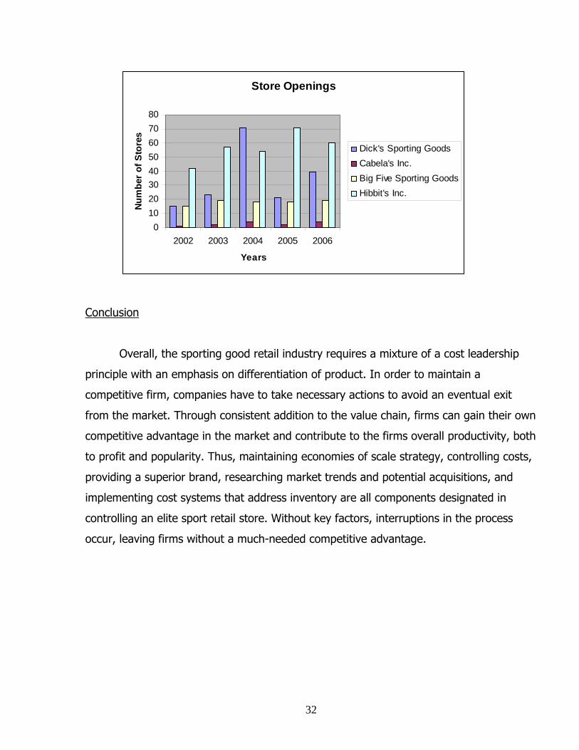
Conclusion

Overall, the sporting good retail industry requires a mixture of a cost leadership

principle with an emphasis on differentiation of product. In order to maintain a

competitive firm, companies have to take necessary actions to avoid an eventual exit

from the market. Through consistent addition to the value chain, firms can gain their own

competitive advantage in the market and contribute to the firms overall productivity, both

to profit and popularity. Thus, maintaining economies of scale strategy, controlling costs,

providing a superior brand, researching market trends and potential acquisitions, and

implementing cost systems that address inventory are all components designated in

controlling an elite sport retail store. Without key factors, interruptions in the process

occur, leaving firms without a much-needed competitive advantage.

33

Firm Competitive Advantage Analysis

Dick’s Sporting Goods is in an industry of high competition. Therefore, their main

business strategies to stay competitive have been unique. This lead Dick’s to adapt the

“store-within –a-store” feature which consists of larger format stores containing five

specialty stores within the store. They have achieved cost leadership by using strategies

such as economies of scale and scope, and lowering input costs. They have also

differentiated themselves by supplying great customer service and investing in brand

image. So really they mixed strategies from both a cost leadership and differentiation

strategies to become competitive advantage over the industry. Using these strategies

their profits have increased during the past five years.

Economies of Scale and Scope

Dick’s Sporting Goods have been expanding all over the United States, now with

stores in 34 states. They went from 22 stores in 1994 to 322 stores today and recently

this year acquiring Golf Galaxy and its 65 stores on February 13, 2007. They have

become America’s largest full-line sporting goods company. Dick’s Sporting Goods direct

competitors are much smaller with fewer stores. Dick’s Sporting Goods competitors

consist of Cabelas, Big 5 Sporting Goods, Hibbett Sporting Goods, and other smaller

privately owned stores. Wal-Mart could be a competitor, but we don’t use them as

competitors because their focus on sporting goods is not very large. Dick’s main concern

is their direct competitors that concentrate on sporting goods. Dick’s Sporting Goods

main advantage is that they have over 1,200 vendors they use. Disruption to supplies

could lead to losses in this retail industry, so Dick’s Sporting Goods has all these vendors

to prevent losses and to make sure they are getting the best prices for their merchandise.

Having all these vendors has enabled Dick’s Sporting Goods to acquire high quality

brands at discount prices to stay competitive. Dicks Sporting Goods does not have one

supplier that provides more than 15% of their inventory.

34

Lowering Input Costs

Dick’s Sporting Goods increase in productivity has allowed them to purchase large

masses of products from their suppliers. This can result in overcrowding merchandise in

their stores which can cause problems and would lead to discounts to customer to avoid

over crowdedness. Therefore, Dick’s Sporting Goods has two large distribution centers.

“We rely on two distribution centers along with a smaller return facility.” (Dick’s 2006

10K) They operate a 601,000 square foot and 725,000 square foot center in

Pennsylvania and in Indiana. Having these distribution centers allows Dick’s to reduce

individual store inventory investment, have a more timely replenishment of store

inventory needs, and reduce transportation costs. (Dick’s 2007 10-K) The sporting goods

retail industry is very seasonal and Dick’s Sporting Goods maintains inventory available

through their distribution centers. Along having distribution centers to minimize costs,

Dick’s has also incorporated a operating system that allows them to replenish their

inventory to maximize their productivity. By having this efficient operating system

enables Dick Sporting Goods to allocate their products more effectively resulting in an

increase their profit margins and reducing expenses on their inventory.

Customer Service

Dick’s Sporting Goods is a sporting goods store that invests money on hiring the

perfect candidates that know their sports to take care of their customers. “We were the

first full-line sporting goods retailer to have active members of the Professional Golfers’

Association working in our stores, and as of February 3, 2007 employed 279 PGA

professionals in our golf departments.” (Dicks 2006 10K) They have also hired bike

technicians to sale their bikes and service them, as well. They have professional fitness

trainers to sell their fitness equipment and inform the customers with the right

information. So customers that shop at Dick’s Sporting Goods are aware of the expertise

and that’s why they shop there.

35

Investment in Brand Image

In order to maintain the loyal customers in their stores, Dick’s has invested on

recognized brands such as Nike, Adidas, Under Armour, and Callaway. They have also

invested on their on brands such as Walter Hagan and Ativa to maintain the loyal ones

and attract new ones. Sports fans usually know what brands they like they stick to them.

Dick’s Sporting Goods is also advertising fan Friday’s to attract the sport’s fan to wear

their favorite teams on jerseys. This simply works for advertisement and the people that

don’t have anything to wear feel the desire to go buy their favorite jerseys.

In order for Dick’s Sporting Goods to stay on the competitive advantage they must

keep innovation with their brand image and quality. Great customer service will

encourage customers to keep shopping and to bring new customers, as well. Dick’s

Sporting goods can not just be differentiated though, they must be aware of the cost

leadership strategies to stay competitive.

Into the Future

Dick’s Sporting Goods is always on the verge of expansion and growth. They

recently acquired Golf Galaxy, which operated 65 stores in 24 states. Dick’s Sporting

Goods went from 22 stores in 1994 to 322 stores in 2007. The sporting retail industry is

steadily growing, but Dick’s Sporting Goods growth has been really increasing fast over

the past years. They hope to keep growing over the years to come. Dick’s Sporting

Goods really invests money on studying where they want to open new stores. They are

very careful on choosing their sites and locations according to the market and availability.

“New stores in new markets, where we are less familiar with the target customer and less

well-known, may face different or additional risks and increased costs compared to stores

operated in existing markets, or new stores in existing markets.” (Dick’s 2007 10K)

Being cautious and aware of the competition has helped them be successful in opening

new store that will stay open.

36

Accounting Analysis

The accounting analysis is a tool used to analyze the success of a certain firm

within the market. The analysis uses financial statements in order to have a better

understanding of how well a business is performing and what its future projection looks

like. There is room within accounting systems for managers to influence financial

statement data, making it important for the analysis to understand this and determine

what a manager “used to signal their proprietary information or what is merely disguised

reality” (Palepu and Healy).

Within the accounting analysis consists of 6 steps used to evaluate certain aspects

of the company’s financial statements. These 6 steps include: identify key accounting

polices, assess accounting flexibility, evaluate actual accounting strategy, evaluate the

quality of disclosure, identify potential red flags, and undo accounting distortions.

Identifying key accounting policies is a way to compare its key success factors and its

potential risk. Next a companies accounting flexibility must be measured. Since not all

companies have the same amount of flexibility due to constraints from accounting

standards, we have to keep this in mind when analyzing a company. If a certain

company has accounting flexibility it can use this to either provide information about its

economic situation or hide its true performance, so an evaluation of accounting strategy

must be performed. It is also important for an analyst to evaluate the quality of

disclosure, because even though managers are required to provide a minimum amount of

disclosure, they do have a considerable amount of say in what is released.

One of the most important steps the analyst will make is identifying possible red

flags that could point to questionable accounting. Finally the analyst will undo accounting

distortions if one feels that the company’s financial statements are misleading or

inaccurate. Using all of these steps will help create a successful accounting analysis.

37

Key Accounting Policies

In the accounting analysis it is important to “identify and evaluate the policies and

the estimates the firm uses to measure its critical factors and risks” (Palepu and Healy).

This step is directly influenced by key success factors and risks within the market. As

mentioned in the Five Forces Model Dick’s Sporting Goods key success factors are

economies of scale, tight cost control, and investment in brand image. Due to the

competitive nature of the sporting goods retail industry cost control becomes the most

significant factor. Brand image is a way for companies to invest in marketing the

company’s name; Dick’s utilizes an approach of big brand names for a competitive price.

Continuous Growth

The highly cost competitive market that is the sporting goods retail industry,

creates an atmosphere where companies must continue to grow and expand in order to

stay competitive in the industry. The chart below shows the comparable store net sale

increase percentage and the number of new stores Dick’s Sporting Goods has opened in

the last 5 years.

Sales Growth 2002 2003 2004 2005 2006Comparable store net sales increase 5.10% 2.10% 2.60% 2.60% 6.00%Number of Stores 141 163 234 255 294

*Calculated using Dick’s 2006 10-K

The chart show that not only is Dick’s Sporting Goods growing its sells, it has also

been expanding its store base over the last several years. As of August 4, 2007 Dick’s

Sporting Goods owns and operates 315 stores across 34 states. They also own Golf

Galaxy, a multi-channel golf specialty retailer, with 77 stores in 29 states (Dick’s 2006 10-

K). This merger took place in February 2007, and shows that Dick’s Sporting Goods is

wanting to expand its company into other parts of the industry. Gaylan’s Trading Inc.

was another merger that took place for the company in 2004. With these mergers and

the expansion of stores Dick’s Sporting Goods has significantly increased its sales growth

38

and net assets. However, because the opening of new stores is dependent on several

different factors there is a certain amount of risk associated with the opening of new

stores. This is something to watch for when dealing with Dick’s Sporting Goods, because

the industry is so seasonal.

Economies of Scale

Dick’s Sporting Goods use a system of store clustering to take advantage of

economies of scale in “advertising, promotion, distribution, and supervisory costs. We

seek to locate stores within separate trade areas within each metropolitan area, in order

to establish long-term market penetration”(Dick’s 2006 10-K). This clustering can be very

effective for their marketing and advertising program, in which they can “employ their

advertising strategy using a cost effective basis through the use of newspapers and local

and national television and radio advertising” (Dick’s 2006 10-K).

Their merchandise planning and allocation systems optimizes distribution of most

products to the stores by taking a combination of historical sales data and forecasted

data at an individual store and item level (Dick’s 2006 10-K). The company believes that

this helps with markdowns taken on merchandise and improves sales on these products.

Dick’s has a couple of distribution centers, which after a purchase is made it is sent

directly from the vendor to the distribution center, where it is processed and then

shipped to the store. All purchases made from vendors are done on a short-term

purchase order basis.

Operating and Capital Leases

Within the retail industry it is common for most companies to use operating leases

with their stores. This has a major benefit for a company since operating leases are not

recorded on the balance sheet, making shareholders believe that they are more cost

efficient. Dick’s Sporting Goods leases all of its stores for lease terms for 10-25 years

with multiple 5 year renewal options and which expire at various dates all the way to

2027 (Dick’s 2006 10-K). Dick’s Sporting Goods does give information in their 10-K about

amounts owed for both on and off balance sheet obligations including operating leases.

39

Operating leases total up to be 2.8 billion dollars due through 2011, this is a very

significant number. Operating leases are by far the largest owed contractual obligation,

with capital leases only amounting to 7.8 million in comparison. Two of Dick’s capital

lease agreements are from the estate of a former stockholder that mature in April 2021.

They also have a capital lease on a store with a fixed interest rate of 10.6% that matures

in 2024 (Dick’s 2006 10-K). It is apparent that Dick’s prefers to use operating leases

over capital leases, which is generally the case in the retail industry.

Goodwill

Dick’s Sporting Goods did record “$156.6 million of goodwill as the excess of the

purchase price of $369.6 million over the fair value of the net amounts assigned to assets

acquired and liabilities assumed” (Dick’s 2006 10-K). This means that sometimes

managers can over estimate the value of a company that is purchased, such as Gaylan’s

and Golf Galaxy, and goodwill is used to balance the balance sheet. Dick’s evaluation of

goodwill for “impairment requires judgments and financial estimates in determining the

fair value of the reporting unit”(Dick’s 2006 10-K). This means that they continually

reevaluate their goodwill to accurately report the difference between the purchase of

Gaylan’s and Golf Galaxy, and this is what these companies are really actually worth.

Conclusion

The key accounting policies a company uses are directly linked to the key success

factors and risks within a market. If an analyst sees that the company’s accounting

policies do not match its success factors then the analyst should be aware of potential

red flags within that companies financials. With Dick’s Sporting Goods we feel like there

is a good amount of information disclosure when dealing with their financials, and they

provided a decent amount of information regarding mergers and their leasing policy.

40

Areas of Accounting Flexibility

The Generally Accepted Accounting Principles (GAAP) is accounting guidelines for

presenting and reporting financial statements. Firms report financial information so that

investors can make informed decisions on future investments. GAAP allows flexible

methods for reporting data that could lead to distortion in the financial data and could

mislead investors, as well. Information reported should be consistent to improve the

quality and credibility of the financial statements. Balance sheets and income statements

have high amount of flexibility that can be manipulated by top management.

Operating vs. Capital Leases

Reporting operating vs. capital leases in one way flexible accounting helps

managers. In the operating lease, “the lessor transfers only the right to use the property

to the lessee (www.cr-ny.com).” The lessee is only renting the property and has no right

of ownership; therefore the lease can be booked as an expense in the income statement.

The booking of this expense would have no effect on the balance sheet and would be

considered an off balance sheet asset. Dick’s Sporting Goods and most of its competitors

have operating leases for most of their stores. Dicks Sporting Goods operating leases

range from 10-25 years. Dicks Sporting Goods only has two buildings that they have

capital leases on. One of these capital leases is the year 2021 and the other is till 2024.

These operating leases are expenses that do not show up on the balance sheets, which

cause the company’s assets and or liabilities to be understated. So with understated

expenses, the company is going to show overstated net income. The overstated of

owners equity and net income makes the company look more profitable and therefore

investors are more willing to invest.

On the other hand, capital leases are treated as paying interest on debt. When

you have capital leases you assume the risk of ownership. Capital leases do affect the

balance sheet, unlike operating leases. “If it is a capital lease, the lessor records the

present value of future cash flows as revenue and recognizes expenses. The lease

receivable is also shown as an asset on the balance sheet, and interest revenue is

recognized over the term of the lease, as paid (www.cr-ny.com).” Capital leases can be

41

listed as assets or liabilities on the financial statements. They show up as assets under

plant, property, and equipment. They can also show up liabilities under lease payments.

Companies use capital leases to benefit some of the tax shelters, depreciation, and

reduction in interest expenses.

Operating and Capital leases can be used by managers in several different ways.

The flexibility of GAAP to allow these reporting methods allows managers to cover up

some of the true numbers of the companies. The methods managers use does not mean

its wrong, but can compensate them by making their company seem more prosperous

and meet certain covenants.

GAAP also allows flexibility in the reporting of goodwill and intangible assets.

“Goodwill and other finite-lived intangible assets are tested for impairment on an annual

basis (Dick’s 2006 10K).” Valuation of goodwill and intangible assets requires estimation

from managers which could have some estimation error. These estimations could lead to

some degree of potential “red flags”. When the carrying value of the assets is greater

than the fair value of the assets, then their assets are going to be impaired. Dick’s

Sporting Goods Company reports in their 10K that they determine the fair value by using

independent appraisals in order to come out with the best estimate.

Actual Accounting Strategy

Financial reporting can have either high or low disclosure. High disclosure is when

a company gives a wide range of information for the public as well as the investor. The

company does not try to hide anything. The company discusses all items in great detail.

Low disclosure is the reporting of items in less detail only to satisfy the GAAP. Each

company has the ability to report their information in a conservative or aggressive basis.

Most companies in the sporting goods industry show a mixture of both conservative and

aggressive along with Dick’s Sporting Goods.

Most of the sporting goods industry report operating leases instead of capital

leases in order to hide the true performance of company. This is one strategy that Dick’s

Sporting Goods uses reporting their data. In 2006 they reported $7.8 million in capital

leases and $205.8 million of operating leases. As mentioned previously operating leases

42

are a significant amount of contractual obligations in comparison to capital leases. Dick’s

favors the use of operating leases over capital leases, which is easily seen through their

building construction method. Reporting of these financial data is considered to be an

aggressive accounting strategy. These accounting objectives are what managers choose

to do to best fit the company as well as to earn incentives.

Dick’s Sporting Goods also allow customers to return their merchandise if it is

defective. Dick’s also gives credit or markdowns on merchandise that is purchased and

later customers find same merchandise at lower prize within a time period. They offer

allowances for customer and suppliers to maintain a positive relationship. The recording

of these reimbursements and markdowns are considered to be a conservative strategy

along the industry’s disclosure in their 10K’s.

All companies in the sporting goods industry also offer define benefit plans. These

define benefit plans have several assumptions they have to make to get a well deserve

rate of return along with well estimated discount rate. Dick’s Sporting Goods offers

employee stock options as well as a retirement savings plan or 401(K). Employees must

have completed 1 year of employment and have reached age of 21 years or older to

receive this benefit. The companies make several changes to the rates they choose

constantly on their reporting. These changes have not seemed to have made an impact

on the numbers though. The numbers have stayed consistently through past years. The

reporting of these expenses is considered to be relatively conservative in the industry. All

of these different ways of reporting are acceptable by GAAP. The accounting strategies

Dick’s implements might cover their true performance, but they actually are doing what

everyone in the industry is doing.

Evaluation of the Quality of Disclosure

For an analyst or an outsider to view a firm’s financial statements, managers

usually have a significantly great impact on the amount of disclosure it will allow analysts

to view. Ultimately the amount of disclosure available reflects how well an outsider can

truly understand how the firm is operating. Firm’s report their status on a continuing

basis such as their quarterly statements referred to 10-Q or their annual statements

43

known as 10-K’s. The subsequent section will give an outlook on the quality and

quantitative analysis of Dick’s Sporting Goods annual report.

Qualitative Analysis

Companies generally use different type of ways to provide adequate disclosures to

the public. Types include: the Letter to the Shareholders which discusses the “firm’s

industry conditions, its competitive position, and management’s plans for the future”

(Palepu and Healy). Another type is footnotes which explain the main accounting policies

companies decide to use and the reasoning behind it. As well as the Management

discussion and Analysis section, this provides information on changes in a firm’s

performance. Analysts use this information in order to view the company’s performance

and future decision. With the added information analysts, shareholders, investors, and

the public can have assurance in the current and future outlook of the company.

In general, managers have an incentive to manipulate their accounting numbers in

order to make the financial reports more favorable. By taking a closer looking at Dick’s

footnotes and Management Discussion and Analysis, analyst are able to see if there are

any distortions in the numbers. Dick’s 10-k was able to mention many important

information concerning operating and capital leases, an area were managers can easily

manipulate numbers. But one of the main disclosures discussed inside the most recent

10-k’s, was the acquisition of other companies. Midway through the year of 2004, Dick’s

Sporting Goods was able to acquire Gaylan’s Trading Company inc., which was another

sporting goods store. Through this acquisition, Dick’s assume responsibility of 48 of

Gaylan’s stores causing a dramatic change in the financials reports for year 2004 and

2005. Dick’s 10-k was able to give an in depth analysis of the change due to this

acquisition, but this is an area were financial statements can be easily distorted. Some of

the main items disclosed regarding this was goodwill. “The transaction is being accounted

for using the purchase method as required by (SFAS)”(Dick’s 2004 10-k). The following

statement displays the amount of goodwill calculated based on purchase acquired taken

into account fair values of assets and liabilities.

44

“In accordance with SFAS No. 141, “Business Combinations.” As of January 29,

2005, $157.2 million of goodwill was recorded as the excess of the purchase price

of $369.5 million over the fair value of the net amounts assigned to assets

acquired and liabilities assumed. In accordance with SFAS No. 142, “Accounting for

Goodwill and Other Intangible Assets,” the Company will continue to assess on an

annual basis whether goodwill and other intangible assets acquired in the

acquisition of Galyan’s are impaired. Additional impairment assessments may be

performed on an interim basis if the Company deems it necessary. Finite-lived

intangible assets are amortized over their estimated useful economic lives and are

periodically reviewed for impairment. No amounts assigned to any intangible

assets are deductible for tax purposes” (Dick’s 2004 10-k/ Management Discussion

Section).

As a result there could be a considerable amount of distortion on the manager’s

behalf. But it seems that Dick’s was able to give an accurate account of the purchase and

goodwill. According to the five year balance sheet, there is a dramatic increase in assets

but goodwill is consistent the following years. Also the income statements do show a

change in net sales but overall there is no erratic change in expense and in net income.

Dick’s Sporting Goods provides good information in their 10-K that is relevant to the key

success factors.

Quantitative Analysis

Transparent Financial Reporting refers to the ability to allow outsiders to acquire a

“true and fair” picture of the firm’s financial statements (Ch 1. Class Notes). But

managers are able to make their judgments on displaying their financial statements

because they have personal comprehension of their company’s operations. In order

words, they have the discretion on to how much information they will present in the

reports. The amount of flexibility that managers have, usually results at a cost. If

managers have a fair amount of flexibility, this tends to make the financial reports less

informative and not reflect their genuine business. On the other hand if managers

45

flexibility is limited, this result in a aggressive financial reports which decreases the

relevance of the valuation. So if the accounting standards are too strict, managers may

be tempted to restructure their business transactions in order to have a higher earnings.

Quantitative analysis allows for a better evaluation of the financial reports numbering.

Quantitative analysis allows for a diagnostic measure to ensure a greater validity

of the financial reports. There are two types of diagnostics that measures the revenues

and expenses incurred year by year. One is the sales manipulation diagnostics which

computes ratios of net sales to cash from sales, net account receivable, unearned

revenues, warranty liabilities, and inventory. These ratios determine if the sales acquired

is accurate. The other type is expense manipulation diagnostic which includes ratios for

declining asset turnover, changes in CFFO/OI, changes in CFFO/NOA, total

accruals/change in sales, pension expense/ SG&A. These ratios determine how well the

firm is managing their expenses.

Core Sales Manipulation Diagnostics

As noted before, managers have a significant impact on the financial reports given

every year. Their incentives drive them to manipulate the numbers in order to show the

reports in their favor. By allowing outsiders the opportunity to view their annual reports,

a thorough analysis can be conducted to observe a company’s true performance. The

following will display a graphical analysis of Dick’s Sporting Goods sales performance

along with the main competitors such as Hibbits, Cabela’s, Big 5 Sporting Goods, and as

well as at an overall industry level. The graph includes ratios for sales manipulation

diagnostics of: Net Sales/ Cash from Sales, Net Sales/ Net Account Receivable, and Net

Sales/ Inventory. Having the following denominator compared to net sales allow analysts

to see if consistency of the reported net sales.

46

Net Sales/ Cash from Sales

Net Sales/ Cash from Sales

0

0.2

0.4

0.6

0.8

1

1.2

2002 2003 2004 2005 2006

Year

DKSHIBBCABBGFVIndustry AVG

The ratio of net sales to cash from sales is a measurement of whether or not a

company’s sales are high in comparison to its cash flow. The computation of this graph

came about by comparing total average net sales of a year to average cash collected

from sells in that year excluding account receivables.

In general a company would prefer a ratio of 1:1, which on average Dick’s is able

to collect cash from sales at a steady rate near 1. This appears to be consistent with the

rest of the industry. It should be noted that there was a net sale increase in year 2004

by 24% due to the acquisition of Gaylan’s stores, which was another sporting goods store

which brought a huge increase in revenue the following year (DKS 10- K). As a result the

ratio jumps from .99 to 1.04 from year 2004 to 2005, indicating that in year 2005 Dick’s

was receiving less cash than products sold. Cabela’s did not release information in a 10-K

for the year 2002, which means that the ratios could not be calculated for both 2002 and

2003, since previous year information is used.

47

Net Sales/ Account Receivables

Net Sales/ Net Account Receivable

0.00

50.00

100.00

150.00

200.00

250.00

2002 2003 2004 2005 2006

Year

DKS

HIBB

CAB

BGFV

Industry AVG

When comparing industry net sales to account receivable ratio each company

appears to maintain a relatively low ratio, with Dick’s Sporting Goods spiking in 2004, but

regaining stability in 2005. This ratio is computed by dividing net sales by account

receivables. The spike in Dick’s ratio in 2004 can be attributed to the merger that took

place between them and Gaylan’s, with Dick’s Sporting Goods taking on their account

receivables. But it started to recede once again after collecting most of the receivables

amount. The amount of account receivables collected primarily through credit cards is

fairly low for Dick’s compared to the total net sales.

Overall, the companies do not seem to keep a consistent ratio, which would raise

the question of whether or not net sales or net accounts receivables were reported

accurately. Cabela’s did not provide a company 10-K in the year 2002, giving the reason

to why that ratio is 0.

48

Net Sales/ Inventory

Net Sales/Inventory

0.002.004.006.008.00

10.0012.0014.00

2002 2003 2004 2005 2006

Year

DKS

HIBB

CAB

BGFV

Industry AVG

The net sales to inventory ratio explains how well companies maintain their

inventory levels to produce profits. This is where the flexibility of inventory methods

really can help companies. This graph shows that Dick’s has maintained a consistent

inventory ratio and therefore explains why they have been profitable. But on the other

hand Big 5 Sporting Goods really increased their ratio from 2005 to 2006. Unexpected

spikes like this could indicate that a company has overstated its Net Sales. As mentioned

previously Cabela’s did not release a 10-K for 2002.

Conclusion

After reviewing the results of the ratios calculated above, it would seem to us that

the reported sales are credible. Dick’s Sporting Goods appears to maintain ratio levels

even with the rest of the industry, and their does not appear to be any spikes on any

charts, which could be a suggestion that sales are not recorded credibly. Due to this we

feel that since their does not appear to be anything to be suspicious over, Dick’s Sporting

Goods did a good job in recording their financial data honestly.

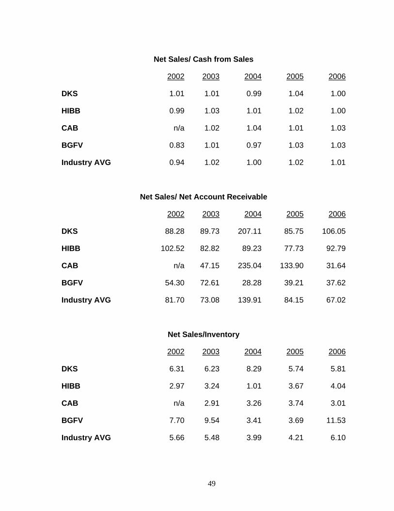
49

Net Sales/ Cash from Sales

2002 2003 2004 2005 2006

DKS 1.01 1.01 0.99 1.04 1.00

HIBB 0.99 1.03 1.01 1.02 1.00

CAB n/a 1.02 1.04 1.01 1.03

BGFV 0.83 1.01 0.97 1.03 1.03

Industry AVG 0.94 1.02 1.00 1.02 1.01

Net Sales/ Net Account Receivable

2002 2003 2004 2005 2006

DKS 88.28 89.73 207.11 85.75 106.05

HIBB 102.52 82.82 89.23 77.73 92.79

CAB n/a 47.15 235.04 133.90 31.64

BGFV 54.30 72.61 28.28 39.21 37.62

Industry AVG 81.70 73.08 139.91 84.15 67.02

Net Sales/Inventory

2002 2003 2004 2005 2006

DKS 6.31 6.23 8.29 5.74 5.81

HIBB 2.97 3.24 1.01 3.67 4.04

CAB n/a 2.91 3.26 3.74 3.01

BGFV 7.70 9.54 3.41 3.69 11.53

Industry AVG 5.66 5.48 3.99 4.21 6.10

50

Core Expense Manipulation Diagnostics

Besides examining the financial reports through a sales manipulation diagnostic,

an expense diagnostics can also be examined to see if there are any discrepancies. By

observing the expenses, one can determine the impact it has on the net income for a

company. Any potential change in expenses can dramatically influence the company’s

overall standing. The following graphs and summaries concentrate on expense

manipulation by Dick’s Sporting Goods, Big 5 Sporting Goods, Cabela’s, and Hibbet.

Asset Turnover

Asset Turnover

0.00

1.002.00

3.004.00

5.00

2002 2003 2004 2005 2006

Year

DKS

HIBB

CAB

BGFV

Industry AVG

By computing the asset turnover ratio, an analyst can see how efficient the firm is

using its assets to generate sales. Having a higher ratio means that a firm is more able to

use its assets to generate money. The graph indicates that Dick’s has consistent asset

turnover ratio until about year 2004. This sudden drop in asset turnover can be

attributed to the merger with Gaylan’s Inc., which would increase assets substantially.

As far as the industry, all competitors seem to be on the same stream, with Dick’s

being the highest. The industry average increased from 2002 to 2003, and decreased

from 2003 to 2004, but is steadily increasing from 2004 to 2006.

51

Change in CFFO/OI

Change in CFFO/ OI

0.000.501.001.502.002.503.00

2002 2003 2004 2005 2006

Year

DKS

HIBB

CAB

BGFV

Industry AVG

The ratio of cash flow from operations over operating income compares how much

cash is generating from cash operations. With this ratio companies want a lower

number. The lower the ratio the better. It seems like Dick’s was struggling in year 2005

or their profits must have came from investing and financing activities since their ratio

was higher than the industry average. Dick’s decreased their ratio very rapidly from 2005

to 2006, which would indicate an increase in profits from operating activities. The

industry average seems to have stayed steady though from 2002 to 2006.

52

CFFO/NOA

Change in CFFO/ NOA

0.00

1.00

2.00

3.00

4.00

2002 2003 2004 2005 2006

Year

DKS

HIBB

CAB

BGFV

Industry AVG

CFFO/NOA

0.00

0.20

0.40

0.60

0.80

2002 2003 2004 2005 2006

Year

DKS

HIBB

CAB

BGFV

Industry AVG

The ratio of cash flow from operations to net operating assets basically relates the

cash from operations to industry’s fixed assets (include property, plant, and equipment).

In general the ratio of CFFO/NOA shows how well a company utilizes property, plant, and

53

equipment to generate cash flows. The higher the ratio indicates more income was

produced during each year from these fixed assets.

Overall Dick’s Sporting Goods runs even with the industry average, but in recent

years all companies have had a decline. This decline is due to higher property, plant, and

equipment compared to a lower growth of cash flows from operations. Another thing we

can conclude is that since most companies in the sporting goods retail industry have

operating leases for most of their stores, then the expense of operating leases brings the

CFFO/ NOA ratio lower. This would explain the higher property, plant, and equipment

numbers.

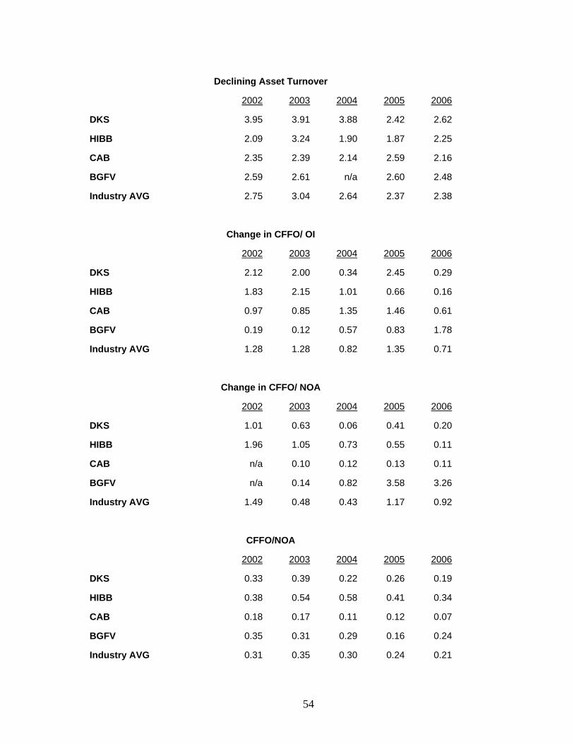
54

Declining Asset Turnover

2002 2003 2004 2005 2006

DKS 3.95 3.91 3.88 2.42 2.62

HIBB 2.09 3.24 1.90 1.87 2.25

CAB 2.35 2.39 2.14 2.59 2.16

BGFV 2.59 2.61 n/a 2.60 2.48

Industry AVG 2.75 3.04 2.64 2.37 2.38

Change in CFFO/ OI

2002 2003 2004 2005 2006

DKS 2.12 2.00 0.34 2.45 0.29

HIBB 1.83 2.15 1.01 0.66 0.16

CAB 0.97 0.85 1.35 1.46 0.61

BGFV 0.19 0.12 0.57 0.83 1.78

Industry AVG 1.28 1.28 0.82 1.35 0.71

Change in CFFO/ NOA

2002 2003 2004 2005 2006

DKS 1.01 0.63 0.06 0.41 0.20

HIBB 1.96 1.05 0.73 0.55 0.11

CAB n/a 0.10 0.12 0.13 0.11

BGFV n/a 0.14 0.82 3.58 3.26

Industry AVG 1.49 0.48 0.43 1.17 0.92

CFFO/NOA

2002 2003 2004 2005 2006

DKS 0.33 0.39 0.22 0.26 0.19

HIBB 0.38 0.54 0.58 0.41 0.34

CAB 0.18 0.17 0.11 0.12 0.07

BGFV 0.35 0.31 0.29 0.16 0.24

Industry AVG 0.31 0.35 0.30 0.24 0.21

55

Potential “Red Flags”

Potential “red flags” surface with respect to analyzing any company in any

industry. These “flags” yield notice to potential accounting discrepancies and questionable

manners in regards to reporting. Although Dick’s Sporting Goods continues to grow at a

vast pace within the market, minimal problems in their accounting strategy exist. With

respect to the two capital leases Dick’s already maintains, the remainder of their leases

are operating. With this in mind, Dick’s liabilities are understated, which leads to a

distorted view on net income. The more off-balance sheet accounting Dick’s involves

itself in the more net income is affected. Currently, the majority of its leases are reported

off the balance sheet as operating leases are the prominent way of running their

business.

On July 29th, 2004, Dick’s Sporting Goods upgraded its market value through the

acquisition of Galyan’s. With this purchase, Dick’s implemented their evaluation of

goodwill for impairment and stated it “requires accounting judgments and financial

estimates in determining the fair value of the reporting unit” (Dick’s 2006 10-k). Not only

did it have to account for $156.6 million of goodwill, it also accounted for Galyan’s

inventory and net sales for the fiscal year ending in 2005. Viewing the income statement

the net sales increased from $1,470,845,000 to $2,109,399,000, which is a significant

increase of roughly $638 million. This increase in net sales throws up the “red flag” and

forces the acquisition to be presented. In addition, inventory increased by about 200

million, also introducing the potential overstatement of net inventory. Therefore, without

prior knowledge of the acquisition, the financial statements are not accurately

represented.

56

The Undoing

To reduce distortions and errors related to the accounting analysis process,

analysts have to change the previous calculations (undo) and re-calculate what is said to

be a more accurate representation of the firm’s numbers. This might affect calculated

ratios, investor’s interests in the company, or overall potential growth of the firm. Thus,

potential profitability introduced to investors is misleading without analyzing the following

distortions.

Failing to expense their capital leases payments raises potential “red flags” and

understates the liabilities. In order to effectively realize the understated liabilities, we

have to offer a capitalized version of the current and future operating lease expenses.

This is possible by discounting the payments at a 10.6% discount rate, which is listed as

the average rate in relation to other similar capital leases on the books.

57

Capitalized Lease at a 10.6 % Discount Rate (in thousands)

Fiscal Year FV Payment PV Factor PV Payment 2007 230,830 0.9042 208,7072008 236,681 0.8175 193,4882009 235,771 0.7392 174,2712010 235,007 0.6683 157,0582011 228,976 0.6043 138,3612012 110,118 0.5463 60,1632013 110,118 0.4940 54,3972014 110,118 0.4466 49,1832015 110,118 0.4038 44,4692016 110,118 0.3651 40,2082017 110,118 0.3301 36,3542018 110,118 0.2985 32,8702019 110,118 0.2699 29,7202020 110,118 0.2440 26,8712021 110,118 0.2206 24,2962022 110,118 0.1995 21,9672023 110,118 0.1804 19,8622024 110,118 0.1631 17,9582025 110,118 0.1475 16,2372026 110,118 0.1333 14,6812027 110,118 0.1205 13,274

Total 1,374,394

*Calculated using Dick’s Sporting Goods 10-K

After calculating the difference in payments of a capital lease versus the current

operating leases, we found a $1.4 billion understatement of liabilities. This is a significant

number, and is considered an aggressive accounting strategy. Therefore, by maintaining

operating leases on the books Dick’s Sporting Goods understates their liabilities by $1.4

billion, which must be adjusted on the balance sheet.

Goodwill must also be considered when undoing accounting distortions. Dick’s

Sporting Goods maintains that throughout the year they check for impairments to

goodwill, claiming that no impairments to goodwill occurred during the years of 2004,

58

2005, and 2006. The value provided on the balance sheet must be assumed to be

correct.

Consequently, interpreting distortions allows analysts to provide an accurate

representation of current numbers that contribute to the firms’ overall key success

factors. Re-estimating the difference in a capital lease versus an operating lease

introduced Dick’s Sporting Goods choice in aggressive accounting and assessed their

main distortion.

59

Financial Analysis, Forecast Financials, and

Cost of Capital Estimations

Financial Analysis

To determine how well a company is doing within a certain industry, many analyst

use ratios to take a firm’s financial statements and break them down into easily analyzed

numbers. These ratios make it easier for the analyst to compare how well a certain

company is doing compared to its competitors. The ratios used in this section can be

broken down into three different groups: liquidity ratios, profitability ratios, and capital

structure ratios.

Liquidity Analysis

Liquidity ratios refer to the ability a company has to pay off its short-terms debts

obligations (Investopedia.com). These ratios become an important issue when a company

decides to borrow money. Creditors or lenders usually analyze these ratios to see if the

company has the ability to convert short-term assets into cash so it can cover its debt.

The major liquidity ratios that used are: current ratios, quick ratio, inventory turnover,

accounts receivables turnover, and working capita turnover. The following graphs and

analysis will further analyze how these ratios are applied.

60

Current Ratio

The current ratio is used as a measurement between current assets (cash, cash

equivalents, receivables, etc.) and current liabilities (short term debts and payables).

This ratio determines how well the company could pay back its short term liabilities, if the

need ever arises. It is important to use a 1:1 ratio to base an analysis of the ratio, which

means that a company has $1 of assets for every $1 of short-term debt.

Dick’s Sporting Goods has maintained a relatively stable current ratio around

1.5:1; this means that Dick’s has $1.50 in current assets for every $1 in short term debt.

Many of Dick’s main competitors are above the 2:1 ratio, which means that Dick’s has

generally been at the bottom of the spectrum when dealing with current ratio.

61

Quick Ratio

The quick ratio measures a companies current assets excluding inventory (cash,

cash equivalents, and receivables) and dividing by its current liabilities. This ratio is a

more accurate assessment of how a company is able to convert its current assets to pay

for short term debt, because inventory can sometimes be hard to convert to cash.

Dick’s Sporting Good’s maintains a quick ratio of around 0.3:1, which means that

Dick’s only has $0.30 of liquid assets for every $1 of short term debts. Compared to the

market Dick’s has increased its quick ratio in recent years, giving it a more desirable

outlook.

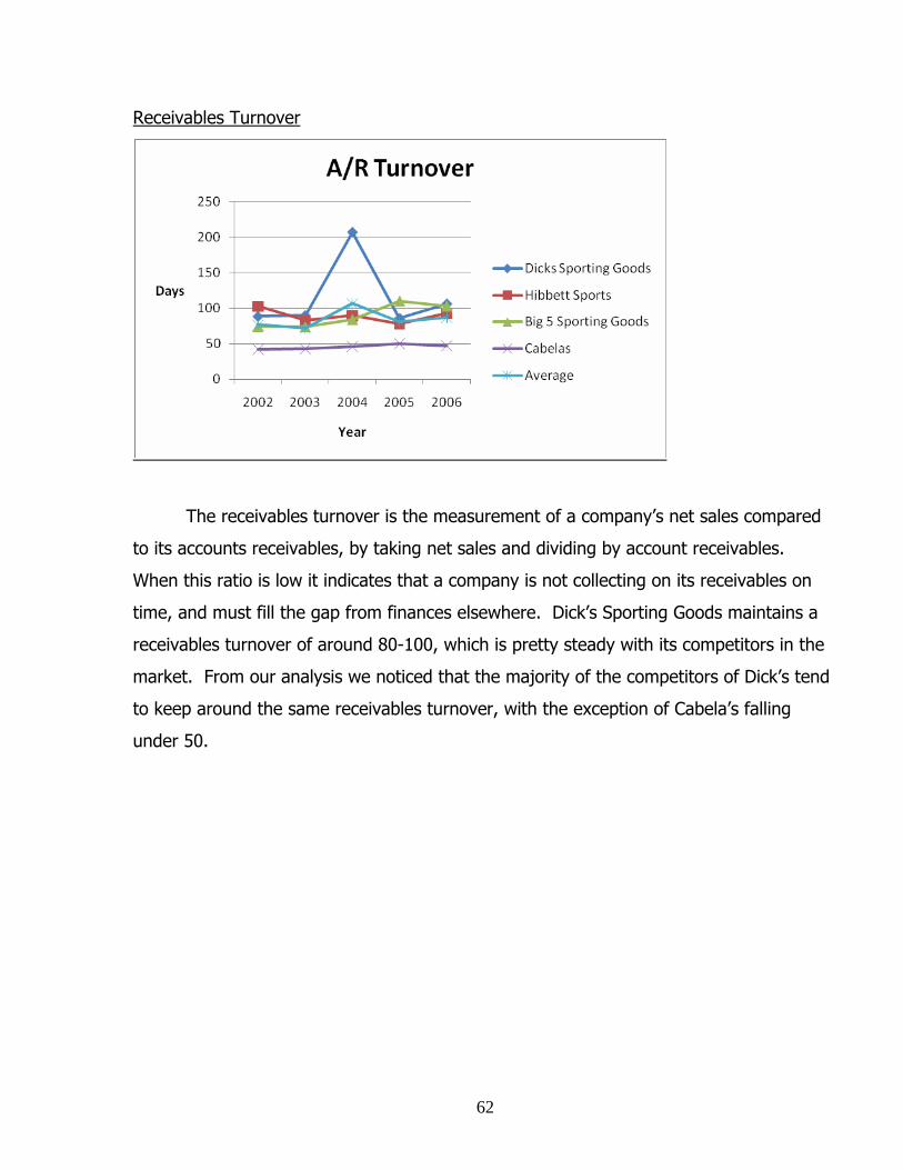
62

Receivables Turnover

The receivables turnover is the measurement of a company’s net sales compared

to its accounts receivables, by taking net sales and dividing by account receivables.

When this ratio is low it indicates that a company is not collecting on its receivables on

time, and must fill the gap from finances elsewhere. Dick’s Sporting Goods maintains a

receivables turnover of around 80-100, which is pretty steady with its competitors in the

market. From our analysis we noticed that the majority of the competitors of Dick’s tend

to keep around the same receivables turnover, with the exception of Cabela’s falling

under 50.

63

Days Sales Outstanding

Days sales outstanding, merely measures how quickly it takes a company to collect

on its accounts receivables. In order to find this analysis, we simply took 365 days in one

year and divide by the receivables turnover ratio calculated. A low number generally

means that a company is doing well, because they are collecting their accounts

receivables quickly. Within the sporting goods retail industry this ratio is typically low

compared to other industries which generally have a 30-90 days sales outstanding ratio.

Dick’s Sporting Goods maintains a days sales outstanding ratio of about 3.5, which means

they collect on their receivables in 3.5 days. As far as the industry, the average days to

collect the receivables are around 3.3 days. So basically Dick’s Sporting Goods are

taking just a bit longer to collect than the industry average which indicates a negative

indication for the company, but is very slim. The faster they collect the faster they can

turn their receivables into cash to reinvest again and able to make more sales. Making

more sales can then generate more profits for the company.

64

Inventory Turnover

The inventory turnover ratio is a measurement of a companies cost of goods sold

compared to its inventory. To find this you simply take the companies cost of goods sold

and divide by the inventory. This ratio tells an analysis how often a company sells and

replaces its inventory. A higher inventory generally indicates that a company has high

sales, but it could also mean that the company has insufficient inventory supply. Dick’s

Sporting Goods is leading the industry in inventory turnover, which indicates that they are

outselling their competitors.

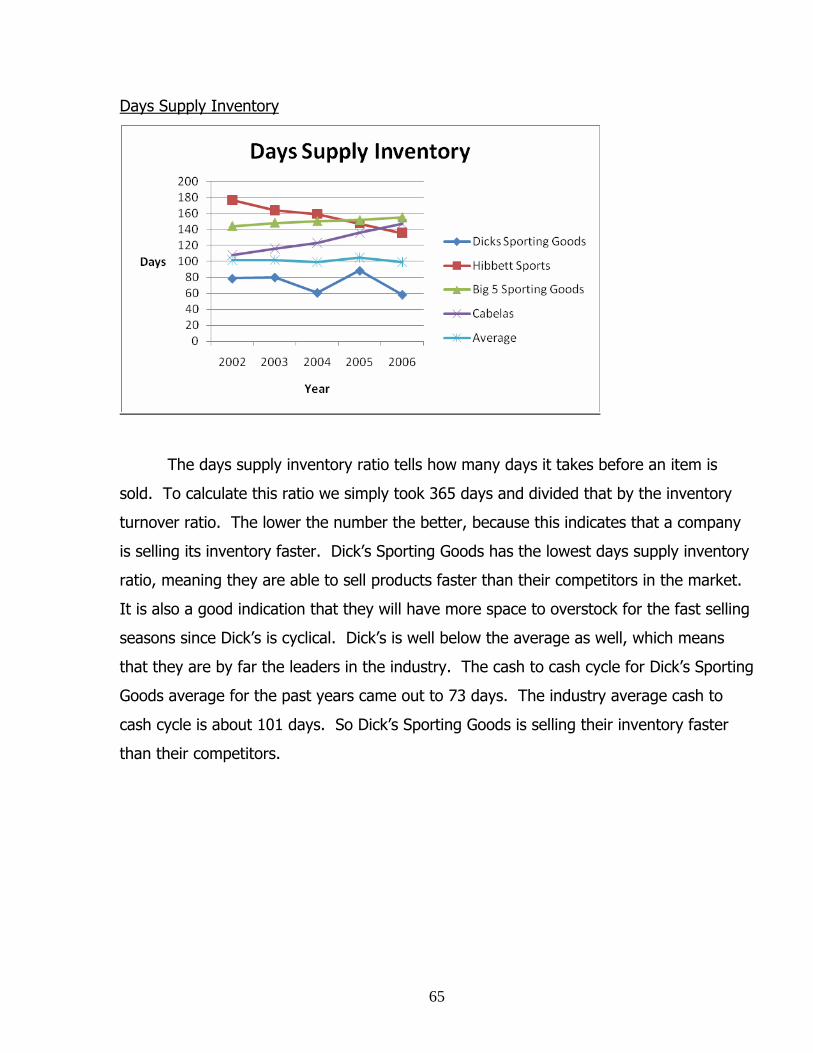
65

Days Supply Inventory

The days supply inventory ratio tells how many days it takes before an item is

sold. To calculate this ratio we simply took 365 days and divided that by the inventory

turnover ratio. The lower the number the better, because this indicates that a company

is selling its inventory faster. Dick’s Sporting Goods has the lowest days supply inventory

ratio, meaning they are able to sell products faster than their competitors in the market.

It is also a good indication that they will have more space to overstock for the fast selling

seasons since Dick’s is cyclical. Dick’s is well below the average as well, which means

that they are by far the leaders in the industry. The cash to cash cycle for Dick’s Sporting

Goods average for the past years came out to 73 days. The industry average cash to

cash cycle is about 101 days. So Dick’s Sporting Goods is selling their inventory faster

than their competitors.

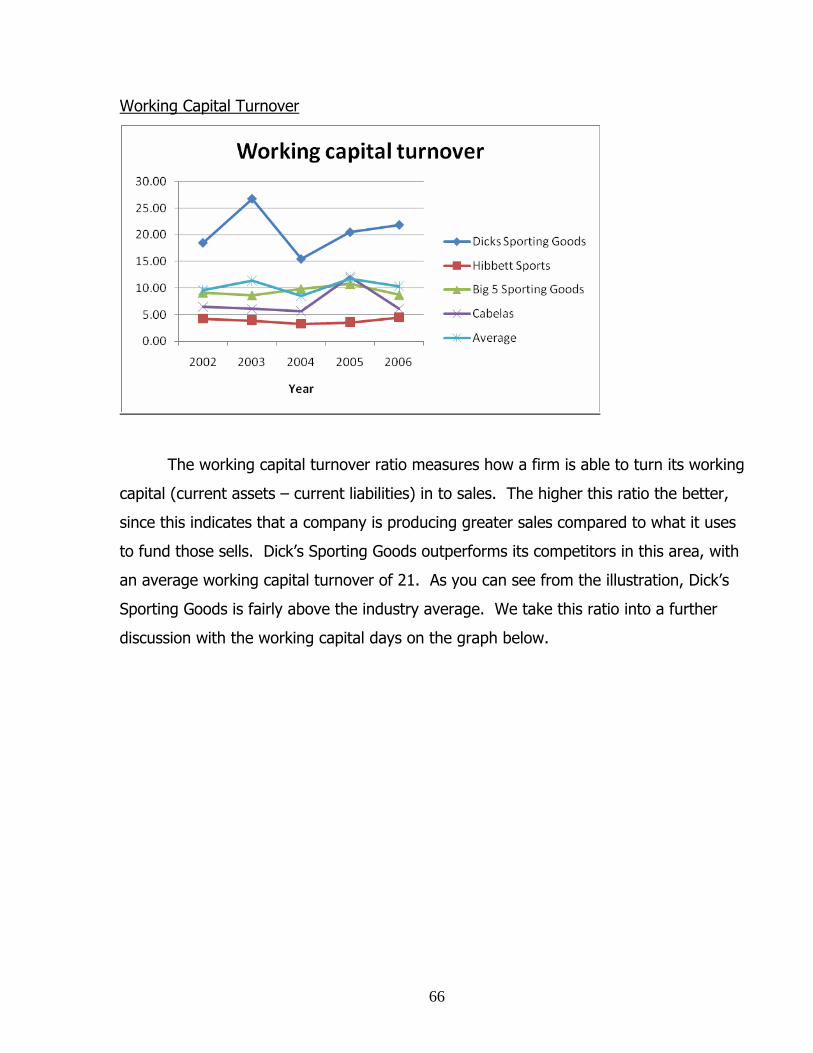
66

Working Capital Turnover

The working capital turnover ratio measures how a firm is able to turn its working

capital (current assets – current liabilities) in to sales. The higher this ratio the better,

since this indicates that a company is producing greater sales compared to what it uses

to fund those sells. Dick’s Sporting Goods outperforms its competitors in this area, with

an average working capital turnover of 21. As you can see from the illustration, Dick’s

Sporting Goods is fairly above the industry average. We take this ratio into a further

discussion with the working capital days on the graph below.

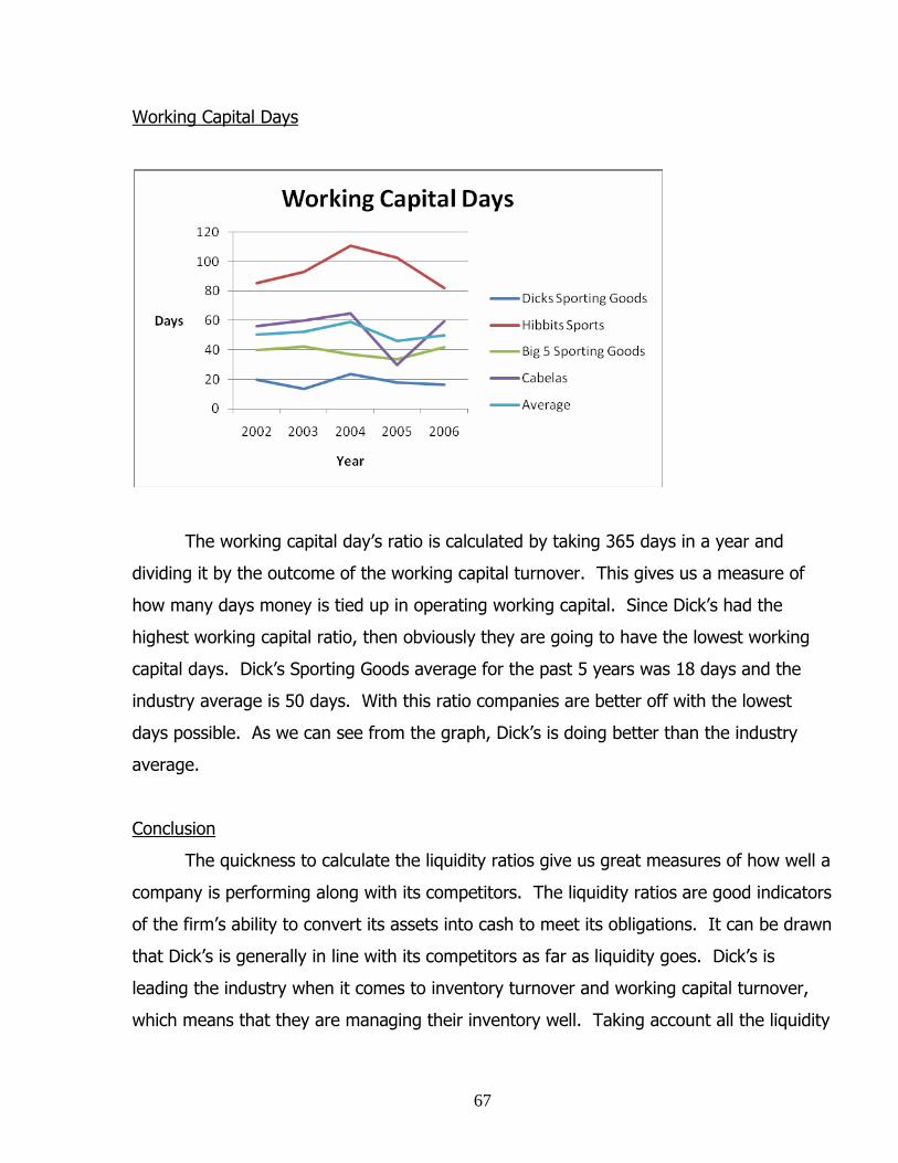
67

Working Capital Days

The working capital day’s ratio is calculated by taking 365 days in a year and

dividing it by the outcome of the working capital turnover. This gives us a measure of

how many days money is tied up in operating working capital. Since Dick’s had the

highest working capital ratio, then obviously they are going to have the lowest working

capital days. Dick’s Sporting Goods average for the past 5 years was 18 days and the

industry average is 50 days. With this ratio companies are better off with the lowest

days possible. As we can see from the graph, Dick’s is doing better than the industry

average.

Conclusion

The quickness to calculate the liquidity ratios give us great measures of how well a

company is performing along with its competitors. The liquidity ratios are good indicators

of the firm’s ability to convert its assets into cash to meet its obligations. It can be drawn

that Dick’s is generally in line with its competitors as far as liquidity goes. Dick’s is

leading the industry when it comes to inventory turnover and working capital turnover,

which means that they are managing their inventory well. Taking account all the liquidity

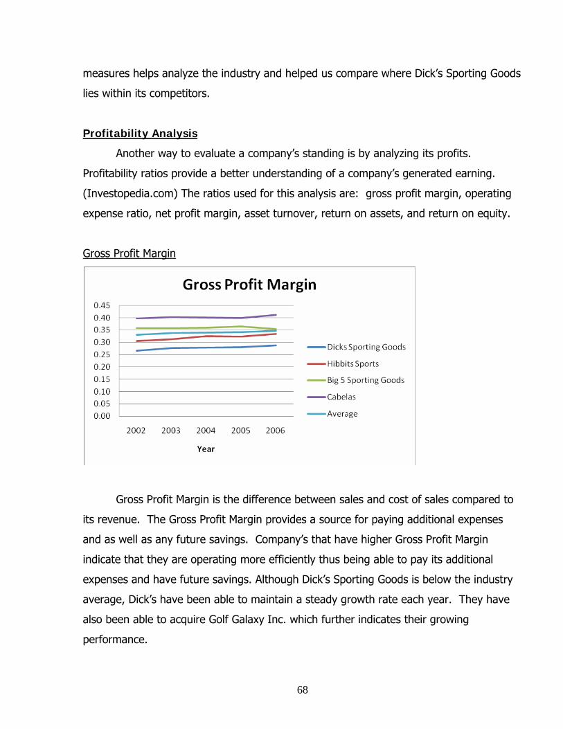
68

measures helps analyze the industry and helped us compare where Dick’s Sporting Goods

lies within its competitors.

Profitability Analysis

Another way to evaluate a company’s standing is by analyzing its profits.

Profitability ratios provide a better understanding of a company’s generated earning.

(Investopedia.com) The ratios used for this analysis are: gross profit margin, operating

expense ratio, net profit margin, asset turnover, return on assets, and return on equity.

Gross Profit Margin

Gross Profit Margin is the difference between sales and cost of sales compared to

its revenue. The Gross Profit Margin provides a source for paying additional expenses

and as well as any future savings. Company’s that have higher Gross Profit Margin

indicate that they are operating more efficiently thus being able to pay its additional

expenses and have future savings. Although Dick’s Sporting Goods is below the industry

average, Dick’s have been able to maintain a steady growth rate each year. They have

also been able to acquire Golf Galaxy Inc. which further indicates their growing

performance.

69

Operating Profit Margin

The company’s income from operations is computed by taking the gross profits

and deducting all the expenses. To evaluate the operating profit margin, take income

form operations and divide by the total sales. This ratio measures how efficient a

company is in maintaining their operating expenses low. This ratio is important to

investors because it shows how well a company is able to have cost control and

minimizing day to day expenses. From analyzing this graph, Dick’s is clearly below the

industry average as well as the main competitors. This low operating profit margin is due

to the Dick’s increasing operating expenses. From the past five years, Dick’s has made

pretty heavy expenditures which is made now in order to increase the company. From

year 2005 to 2006, it’s clearly to see that Dick’s operating profit margin is increasing

indicating that profits are increasing as well.

70

Net Profit Margin

Net Profit Margin indicates how well the company was able to control its cost. In

other words how well a company was able to convert revenue into profit after deducting

all of the cost or expenses incurred throughout the year. The higher the percentage the

better a company is able to keep its earnings. Net Profit Margin is calculated by dividing

Net Income by its sales. Dick’s Net Profit Margin begins to downward slope around 2003

after the acquisition of Gaylan’s Golf Galaxy. The downward sloping can be attributed to

the extra cost of the acquisition as well having expenses in expanding to other stores. At

year 2005, the Net Profit Margin starts to increase from about 2.8 to 3.5 which is due to

the dramatic increase in net income in that year indicating that Dick’s is becoming more

profitable.

71

Asset Turnover

The Asset Turnover is “used to determine how much sales revenue a company

generates from its investment in assets”(Wikepedia.com). The Asset Turnover ratio or

sales divided by assets, is a good indicative of how well a company is able to convert

asset into revenue. As the graph indicates, Dicks is above the industry’s average as well

as all of the other main competitors. There is a dramatic drop from year 2004 to 2005

primarily due to the acquisition of Gaylans Golf Galaxy. In that year sales maintain a

steady growth but asset increase almost twice its size from $543360 to $1085048. But

then in year 2005 the asset turnover rate begins to increase passing all of our main

competitors.

72

Return on Assets

Return on assets tells how profitable a company is relative to its total assets.

(Investopedia.com) The ROA shows how much earnings were earned from its assets.

ROA is computed by dividing the net income by the total assets of the year before. This

ratio is important because it shows how well the company is able to turn their investment

in every asset they put in into profit. The higher the return on assets, the better the

company is doing in making profits in its assets with fewer investments. The reason for

Dick’s start off point is in year 2003, is the data for year 2001 was not provided. Dick’s

return on asset is above all of the other competitors just under 2 percent. After year

2004 there is a decline in ROA due to the increase in total assets.

73

Return on Equity

Return on Equity is one of the most important ratios because it explains the

company’s performance. ROE demonstrates how well a company was able to produce a

profit through its earnings. Divide the total net income by its total owner’s equity to get

the ROE ratio. Year 2001 information was not disclosed for these companies’ and

therefore we were not able to compute the year 2002 ratios. The graph indicates that

Dick’s is below industry average right below 1 percent. Dick’s is moving along the

industry’s average which is a good indicator that they are doing well in the industry. The

declining rate for Dick’s is mainly due to the decreasing amount in owner’s equity

attributed to the acquisition of other stores.

Return on Equity

0

1

2

3

4

5

6

7

2002 2003 2004 2005 2006Year

Dicks Sporting Goods

Hibbett SportsBig 5 Sporting Goods

CabelasAverage

74

Conclusion

The profitability ratios are great ways to measure if a firm is creating revenue.

Some of these ratios also compare their revenues to its operating expenses. The

profitability ratios are easy created from the financial statements and helped us compare

Dick’s Sporting Goods to its competitors. These profitability ratios helped us examine

benchmarks of the industry to make assumptions on Dick’s profitability.

Capital Structure Analysis

There are three capital structure ratios used to evaluate the strength of Dick’s

Sporting Goods compared to its competitors along the industry. The first one is the debt

to equity ratio calculated by the total liabilities divided by the total owners’ equity. The

second ratio is the times interest earned computed by the operating income divided by

the interest expense. The last ratio is the debt service margin ratio computed by the

currents year cash flow from operations divided by the previous year notes payable. All

of these ratios and illustrations help us in our valuations of Dick’s Sporting Goods and are

further discussed.

Debt to Equity

Debt to Equity refers to the amount of debt company uses produce revenue. Debt

to Equity is calculated by taking the total liabilities divided by the total owner’s equity.

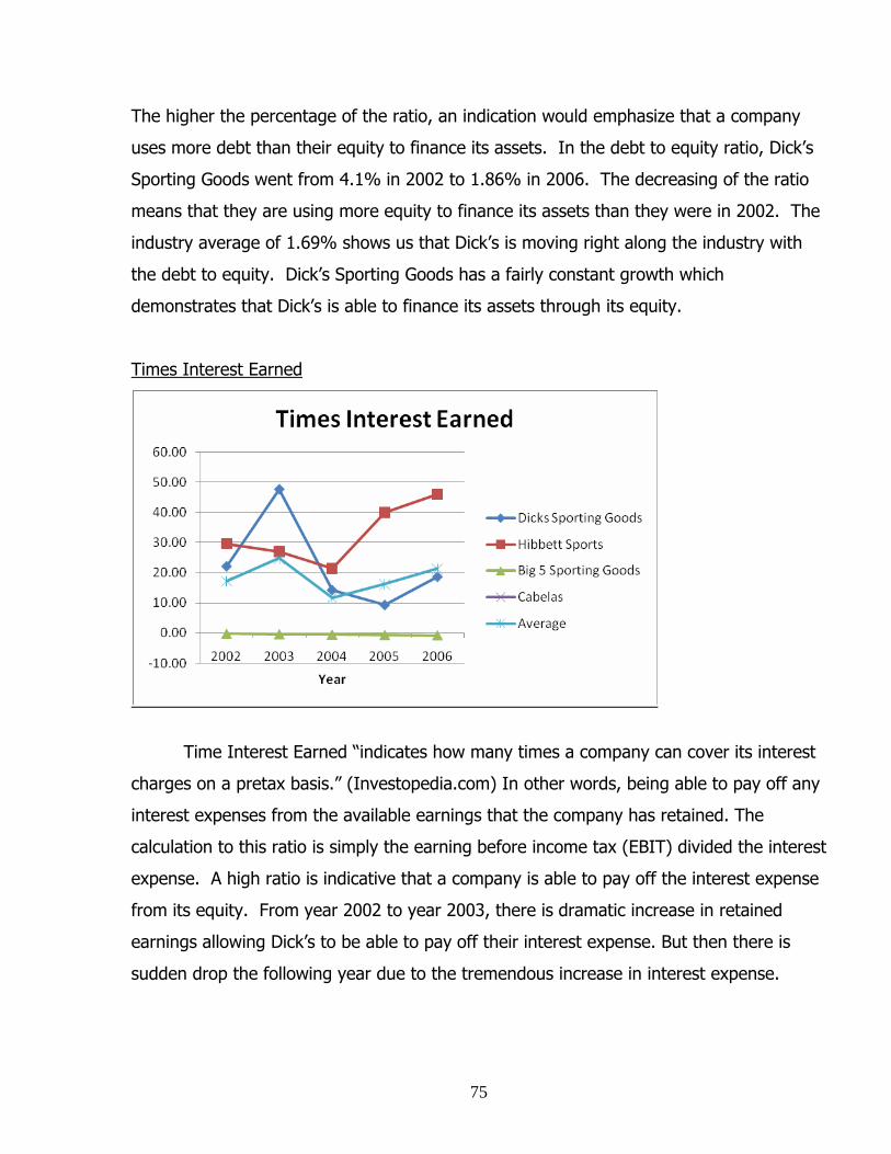
75

The higher the percentage of the ratio, an indication would emphasize that a company

uses more debt than their equity to finance its assets. In the debt to equity ratio, Dick’s

Sporting Goods went from 4.1% in 2002 to 1.86% in 2006. The decreasing of the ratio

means that they are using more equity to finance its assets than they were in 2002. The

industry average of 1.69% shows us that Dick’s is moving right along the industry with

the debt to equity. Dick’s Sporting Goods has a fairly constant growth which

demonstrates that Dick’s is able to finance its assets through its equity.

Times Interest Earned

Time Interest Earned “indicates how many times a company can cover its interest

charges on a pretax basis.” (Investopedia.com) In other words, being able to pay off any

interest expenses from the available earnings that the company has retained. The

calculation to this ratio is simply the earning before income tax (EBIT) divided the interest

expense. A high ratio is indicative that a company is able to pay off the interest expense

from its equity. From year 2002 to year 2003, there is dramatic increase in retained

earnings allowing Dick’s to be able to pay off their interest expense. But then there is

sudden drop the following year due to the tremendous increase in interest expense.

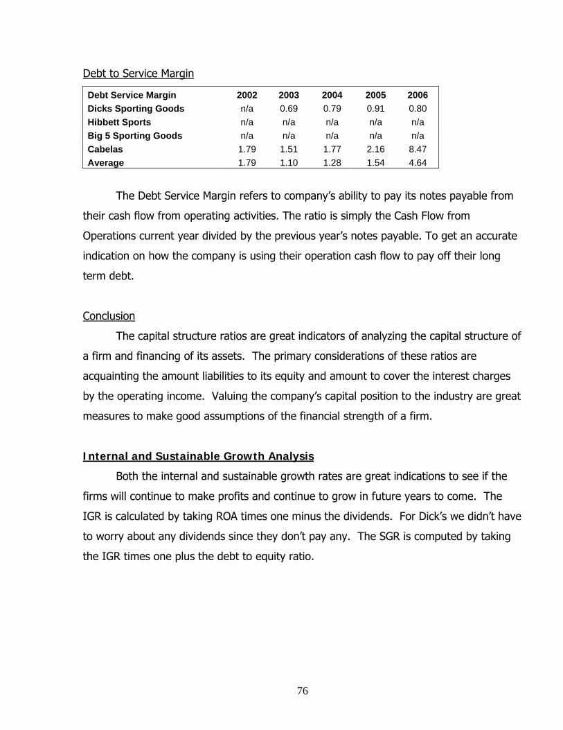
76

Debt to Service Margin

Debt Service Margin 2002 2003 2004 2005 2006 Dicks Sporting Goods n/a 0.69 0.79 0.91 0.80 Hibbett Sports n/a n/a n/a n/a n/a Big 5 Sporting Goods n/a n/a n/a n/a n/a Cabelas 1.79 1.51 1.77 2.16 8.47 Average 1.79 1.10 1.28 1.54 4.64

The Debt Service Margin refers to company’s ability to pay its notes payable from

their cash flow from operating activities. The ratio is simply the Cash Flow from

Operations current year divided by the previous year’s notes payable. To get an accurate

indication on how the company is using their operation cash flow to pay off their long

term debt.

Conclusion

The capital structure ratios are great indicators of analyzing the capital structure of

a firm and financing of its assets. The primary considerations of these ratios are

acquainting the amount liabilities to its equity and amount to cover the interest charges

by the operating income. Valuing the company’s capital position to the industry are great

measures to make good assumptions of the financial strength of a firm.

Internal and Sustainable Growth Analysis

Both the internal and sustainable growth rates are great indications to see if the

firms will continue to make profits and continue to grow in future years to come. The

IGR is calculated by taking ROA times one minus the dividends. For Dick’s we didn’t have

to worry about any dividends since they don’t pay any. The SGR is computed by taking

the IGR times one plus the debt to equity ratio.

77

Internal Growth Rate

IGR is the “growth that a company can reach without having to use any financing

(www.investopedia.com).” Calculating these growths rate helped us determine how fast

Dick’s Sporting Goods is really growing. The IGR growth rate that we came up for Dick’s

was an average of 14.6 percent for IGR and so we can conclude that Dicks has this

percentage of growth potential. The industry average was around 10 percent and Dick’s

Sporting Goods have been above the industry average on growth potential which is a

good indication of how fast they are growing. The actual growth for Dick’s is around 3.2

percent along with the industry actual growths provided from the 10-K financials.

78

Sustainable Growth Rate

The SGR is the “maximum growth that a company can sustain without having to

use financial leverage (www.investopedia.com).” Since Dick’s does not pay any dividends

our calculations were much easier. Dick’s Sporting Goods average SGR came out to

about 39.08 percent for past 5 years. The industry average was around 22.90 percent.

This tells us that Dick’s is growing at a very fast pace, but we didn’t think this was an

accurate number for our estimations for our forecasts. Since the industry actual growth

rate are between 3 to 4 percent we decided to forecast our net sales at a conservative 5

percent throughout the 10 years forecasted. We used a 5 percent because we believe

Dick’s is growing a little faster than the industry average. We can see a better picture

from the illustrations of our IGR and SGR graphs.

Conclusion

Both the IGR and SGR ratios play a major role to determine the profitability of a

firm. When both ratios are higher we can conclude that companies have less debt

obligations and there probably finance most of their debt from their equity. By doing this

companies will be more profitable in future years. As we saw the illustrations from the

graphs, we can see that Dick’s Sporting Good’s IGR and SGR are fairly higher than their

79

competitors. We can assume that Dick’s will be profitable in the future by observing

these ratios.

Financial Statement Forecasting Methodology

Forecasting future years for a firm’s financial statements provides bigger picture

and understanding in the valuing of a firm. In the forecasting process to forecast the

financials for 10 years of future data we had to look for trends in the financials and on

the ratios we discussed earlier. By looking for trends in the balance sheet, income

statement, and the cash flows was a good approach to begin making the future

forecasts. We looked for trends in the liquidity ratios, profitability ratios, and capital

structure ratios for Dicks Sporting Goods in order to determine what line items to forecast

in future years. We also calculated the ratios for the competitors that way we could

compare the data of Dick’s Sporting Goods with the industry to make sure our estimates

were fair and reasonable.

We first began with the income statement using the growth rates of the industry

and Dick’s to make assumptions of how fast Dick’s is growing. We also built a common

size income statements, common size balance, and common size cash flows and used

the past 5 year averages for the future forecast for some of the lines items. We mainly

used the ratios for the balance sheet forecasting that was relevant and made sense. For

the statement of cash flows we used the manipulation core expense ratios to make our

determinations at what percent to grow the most relevant items. We further discuss our

financial statements forecasting for the next 10 years.

Forecasting of Income Statement

Forecasting the Income Statement was the first financial statement that we started

to forecast 10 years into the future. We first created a common size income statement

and set our biggest number net sales equal to 100 percent to get all our line items as a

percentage of sales. To forecast our net sales we assumed the rate of 5 percent

80

throughout the next 10 years. Dick’s actual growth rate was 3.2 provided by the 10-K

and the industry growth rate was between 3 to 4 percent. So we assumed that Dick’s

was growing a little above the industry average and so we grew net sales by 5 percent.

We calculated our internal growth rate average for the past four years to be at 14.6

percent and the sustainable growth average at 39.08. We concluded though that this

growth rates were not very reasonable for the forecasting of net sales. The further we

move to the future years the more noise and error there is in the forecasts because we

can’t compare future years with current data that is relevant.

The next thing we forecasted was the cost of goods sold. To forecast cost of

goods sold we took the average of the percentage of the common size income statement

of cost of goods sold for the past 5 years. We came up with 72.21 percent and so we

assumed that was a fair estimate to come up with the future years. So we forecasted the

next 10 years using this estimate. After this we just subtracted cost of goods sold from

net sales to get gross profit so that our statements made sense.

We then forecasted the rest of the line items that were consistent in the last 5

years actual income statements. Some of the line items were not forecasted because

they did not show any trend and were just misleading to the other items. The two lines

items that were not forecasted were pre-opening expenses and store closing costs. Dick’s

pre-opening expense was so low that it did not make any sense in the forecasting. As for

the store closing costs, we only had data for two years out the past 5 years so this was

not very consistent. As far as the rest of the line items, we were able to forecast them all

using the past 5 year’s average. We used the same method using the average of the

common size percentages because we saw we were coming up with good future

estimates.

Dick's Sporting Goods, Inc. 2006 10-k

Forcasted Income Statement

Fiscal Year 2001 2002 2003 2004 2005 2006 Assume Average 2007 2008 2009 2010 2011 2012 2013 2014 2015 2016(Dollars in thousands, except per share)

Statement of Income Data: 0.05

Net sales 893,396 1,272,584 1,470,845 2,109,399 2,624,987 3,114,162 5.00% 100.00% 3,269,870 3,433,364 3,605,032 3,785,283 3,974,548 4,173,275 4,381,939 4,601,036 4,831,087 5,072,642

Cost of goods sold (1) 684,552 934,956 1,062,820 1,522,873 1,887,347 2,217,463 72.21% 2,361,173 2,479,232 2,603,193 2,733,353 2,870,021 3,013,522 3,164,198 3,322,408 3,488,528 3,662,955

Gross profit 208,844 337,628 408,025 586,526 737,640 896,699 27.79% 908,697 954,132 1,001,838 1,051,930 1,104,527 1,159,753 1,217,741 1,278,628 1,342,559 1,409,687

Selling, general and administrative expenses 169,392 262,755 314,885 443,776 556,320 682,625 21.24% 694,520 729,246 765,709 803,994 844,194 886,404 930,724 977,260 1,026,123 1,077,429

Merger integration and store closing costs 20,336 37,790

Pre-opening expenses 5,911 6,000 7,499 11,545 10,781 16,364

Income from operations 33,541 68,873 85,641 110,869 132,749 197,710 5.58% 182,459 191,582 201,161 211,219 221,780 232,869 244,512 256,738 269,575 283,053

(Gain) on sale / loss on write-down of non-cash 2,447 (3,536) (10,981) (1,844)

investment (2) (3)

Interest expense, net 6,963 2,864 1,831 8,009 12,959 10,025 0.31% 10,137 10,643 11,176 11,734 12,321 12,937 13,584 14,263 14,976 15,725

Other income (1,000)

Income before income taxes 26,578 63,562 87,346 114,841 121,634 187,685 5.41% 176,900 185,745 195,032 204,784 215,023 225,774 237,063 248,916 261,362 274,430

Provision for income taxes 10,631 25,425 34,938 45,936 48,654 75,074 2.16% 70,629 74,161 77,869 81,762 85,850 90,143 94,650 99,382 104,351 109,569

Net income 8,643 38,137 52,408 68,905 72,980 112,611 3.24% 105,944 111,241 116,803 122,643 128,775 135,214 141,975 149,074 156,527 164,354

Forecast Financial StatementsActual Financials

Common Size Income Statement

Average

Fiscal Year 2002 2003 2004 2005 2006 2007 2008 2009 2010 2011 2012 2013 2014 2015 2016(Dollars in thousands, except per share and sales per square foot data)

Statement of Income Data:

Sales Growth PercentNet sales 100% 100% 100% 100% 100% 100% 100% 100% 100% 100% 100% 100% 100% 100% 100%

Cost of goods sold (1) 73.47% 72.26% 72.19% 71.90% 71.21% 72.21% 72.21% 72.21% 72.21% 72.21% 72.21% 72.21% 72.21% 72.21% 72.21% 72.21%

Gross profit 26.53% 27.74% 27.81% 28.10% 28.79% 27.79% 27.79% 27.79% 27.79% 27.79% 27.79% 27.79% 27.79% 27.79% 27.79% 27.79%

Selling, general and administrative expenses 20.65% 21.41% 21.04% 21.19% 21.92% 21.24% 21.24% 21.24% 21.24% 21.24% 21.24% 21.24% 21.24% 21.24% 21.24% 21.24%

Merger integration and store closing costs 0.96% 1.44%

Pre-opening expenses 0.0047 0.0051 0.0055 0.0041 0.0053

Income from operations 5.41% 5.82% 5.26% 5.06% 6.35% 5.58% 5.58% 5.58% 5.58% 5.58% 5.58% 5.58% 5.58% 5.58% 5.58% 5.58%

(Gain) on sale / loss on write-down of non-cash 0.19% -0.24% -0.52% -0.07%

investment (2) (3)

Interest expense, net 0.23% 0.12% 0.38% 0.49% 0.32% 0.31% 0.31% 0.31% 0.31% 0.31% 0.31% 0.31% 0.31% 0.31% 0.31% 0.31%

Other income

Income before income taxes 4.99% 5.94% 5.44% 4.63% 6.03% 5.41% 5.41% 5.41% 5.41% 5.41% 5.41% 5.41% 5.41% 5.41% 5.41% 5.41%

Provision for income taxes 2.00% 2.38% 2.18% 1.85% 2.41% 2.16% 2.16% 2.16% 2.16% 2.16% 2.16% 2.16% 2.16% 2.16% 2.16% 2.16%

Net income 3.00% 3.56% 3.27% 2.78% 3.62% 3.24% 3.24% 3.24% 3.24% 3.24% 3.24% 3.24% 3.24% 3.24% 3.24% 3.24%

Forecast Financial Statements

Revised Income Statement

To compute the actual and forecasted years with capital leases corrections we had

to first undo the corrections for our past 5 years data. After we corrected our financials

and came out with corrected numbers, then we were able to move on to the forecast.

We still followed the same format as we did the regular income statement. We did a

common size income statement and used the past 5 years average. We set our net sales

to 100% and every line item as a percentage of sales to get close estimates. We saw

that the difference in net income due to capitalization from years 2001 to 2012 were all

negative numbers due to the fact of capital leases. From 20012 to 2016, we came out

with some positive numbers as Dick’s pays more and more of their capital leases. We

posted this in our Appendix.

Forecasting of Balance Sheet

The forecasting of the balance sheet shows more accuracy in confidence in terms

of confidence and error. The more recent forecasted years will also show better

accuracy. The latest years into the future will have more error in estimation. We made a

common size balance sheet for our balance sheet financials as well as looked at the ratios

discussed earlier. We set our total assets to 100 percent and our total liabilities and

equity to 100 percent so that we wouldn’t have trouble balancing our financials. We then

forecasted total assets by using the asset turnover ratio. We came up with an average of

3.36 percent for the past 5 years and so that is how we came up with the calculations.

We determined that was the best measure because the asset turnover is calculated using

the biggest number in the income statement, net sales divided by the biggest number in

the balance sheet, total assets. This ratio best links the income statement to the balance

sheet and helped us get a fairly accurate estimate. In 2006 we had 1.187 billion in

assets and came up with 1.227 billion in 2007.

To forecast our inventory we assumed that the best indicator would be our

inventory turnover ratio to calculate the best estimate for the next 10 years. We took the

average of past 5 years since they all had a trend and used the 5.1 percent to come up

with the forecasts for inventory. We did the same for the accounts receivables. We took

83

the average of the day’s supply of receivables to come up with best estimate in

calculating the accounts receivable for the next 10 years. We assumed the 3.2 percent

and grew the rest of the years using this ratio in mind.

For the forecast of the liabilities we kind of went the same route as the assets

section. We looked for trends in the financials and trends on the results from the ratios.

If we thought there was no trend then we decided not to forecast the line item. We

forecasted the most important line items starting with our total liabilities and equity.

Since our total assets have to equal our total liabilities and equity results we decided to

use the same growth percent used to calculate the total assets. The 3.36 percent was

used in this calculation and gave us the best estimate in forecasting 10 years out for

Dick’s Sporting Goods.

After this, we moved on to the current liabilities and felt that the current ratio gave

us the best indication to forecast our line item. The average current ratio for the past 5

years was 1.37 percent so we assumed a 1.4 percent would be an accurate number in

estimating 10 years out. For our total liabilities we used the common size average for the

past 5 years times our total liabilities and equity to get our estimates. After getting our

total liabilities, then we were able to get our long term liabilities by subtracting the

current liabilities from our total liabilities. We did the same with our stockholder’s equity.

Since we had already forecasted the total liabilities, then we just subtracted the total

liabilities from total liabilities and equity to get our stockholder’s equity. By doing this, we

were able to keep our balance sheet financials in balance at the end of the process.

Dick's Sporting Goods Balance Sheet2002 2003 2004 2005 2006 Average Assume 2007 2008 2009 2010 2011 2012 2013 2014 2015 2016

ASSETS

CURRENT ASSETS:

Cash and cash equivalents $8,976 $11,120 $93,674 $18,886 $365,464

Accounts receivable, net $14,416 $16,391 $10,185 $30,611 $29,365 3.2 3.2 30,305 31,274 32,275 33,308 34,374 35,474 36,609 37,780 38,989 40,237

Income tax receivable $232 $7,202

Inventories, net $201,585 $233,497 $254,360 $457,618 $355,698 5.1 5.1 373,839 392,904 412,942 434,003 456,137 479,400 503,849 529,545 556,552 584,936

Prepaid expenses and other current assets $5,219 $5,572 $5,222 $8,772 $11,961

Deferred income taxes $5,243 $8,697 $1,021 $7,966 $429

Total current assets $235,439 $275,277 $364,694 $531,055 $614,017 51.00% 626,126 647,164 668,909 691,384 714,615 738,626 763,444 789,095 815,609 843,013

PROPERTY AND EQUIPMENT, NET $71,795 $80,109 $144,402 $349,098 $370,277

CONSTRUCTION IN PROGRESS - LEASED FACILITIES $10,927 $15,233 $7,338

GOODWILL $157,245 $156,628

OTHER ASSETS:

Deferred income taxes $5,970 $7,512 $6,099 $871 $8,959

Investments $5,770 $1,950 $7,054 $3,388 $3,197

Other $3,008 $11,378 $10,184 $28,158 $27,373

Total other assets $14,748 $20,840 $23,337 $32,417 $39,529 601,572 621,785 642,677 664,271 686,591 709,660 733,505 758,150 783,624 809,954

TOTAL ASSETS $321,982 $376,226 $543,360 $1,085,048 $1,187,789 3.36% 1,227,699 1,268,949 1,311,586 1,355,655 1,401,205 1,448,286 1,496,948 1,547,246 1,599,233 1,652,967

LIABILITIES AND STOCKHOLDERS' EQUITY

CURRENT LIABILITIES:

Accounts payable 95,573 125,208 118,383 211,685 253,395

Accrued expenses 47,012 59,239 72,090 141,465 136,520

Deferred revenue and other liabilities 17,958 22,752 37,037 48,882 62,792

Income taxes payable 5,728 12,763 18,381

Current portion of other long-term debt 211 213 505 635 181

Total current liabilities 166,482 220,175 228,015 402,667 471,269 1.40% 471,269 477,867 484,557 491,341 498,219 505,195 512,267 519,439 526,711 534,085

LONG-TERM LIABILITIES:

Senior convertible notes 172,500 172,500

Revolving credit borrowings 77,073 76,094

Other long-term debt 3,577 3,364 3,411 8,775 8,520

Non-cash obligations for construction in progress - leased facilities 10,927 15,233 7,338

Deferred revenue and other liabilities 11,745 12,188 60,113 96,112 113,369

Total long-term liabilities 92,395 15,552 74,451 368,714 301,727

Total Liabilities 258,877 235,727 302,466 771,381 772,996 66.98% 822,313 849,942 878,500 908,018 938,527 970,062 1,002,656 1,036,345 1,071,166 1,107,158

COMMITMENTS AND CONTINGENCIES

STOCKHOLDERS' EQUITY:

Preferred stock, par value, $.01 per share, authorized shares 5,000,000; none issued and outstanding

Common stock, par value, $.01 per share, authorized shares 200,000,000; issued and outstanding

shares 36,545,332 and 34,790,358, at January 28, 2006and January 29, 2005, respectively 169 126 331 348 365Class B common stock, par value, $.01 per share, authorized shares 40,000,000; issued and

outstanding shares 13,730,945 and 14,039,529, at January 28, 2006 and January 29, 2005, respectively 77 141 140 137

Additional paid-in capital 96,279 130,071 175,748 181,321 209,526

Retained earnings 28,029 10,225 60,957 129,862 202,842 202,544 216,463 216,623 231,015 231,663 246,561 247,732 263,169 264,898 280,912

Notes receivables for common stock 6,196

Accumulated other comprehensive income 892 3,717 1,996 1,923

Total stockholders' equity 63,105 140,499 240,894 313,667 414,793 405,386 419,007 433,086 447,637 462,678 478,224 494,292 510,901 528,067 545,810

TOTAL LIABILITIES AND STOCKHOLDERS' EQUITY 321,982 376,226 543,360 1,085,048 1,187,789 3.36% 1,227,699 1,268,949 1,311,586 1,355,655 1,401,205 1,448,286 1,496,948 1,547,246 1,599,233 1,652,967

Actual Financial Statements Forecast Financial Statements

86

Balance Sheet Common Size2002 2003 2004 2005 2006 Average Assume

ASSETS

CURRENT ASSETS:

Cash and cash equivalents 2.79% 2.96% 17.24% 1.74% 30.77% 11.10% 11.50%

Accounts receivable, net 4.48% 4.36% 1.87% 2.82% 2.47% 3.20% 3.20%

Income tax receivable 0 0 0.04% 0.66% 0

Inventories, net 62.61% 62.06% 46.81% 42.17% 29.95% 48.72% 49.00%

Prepaid expenses and other current assets 1.62% 1.48% 0.96% 0.81% 1.01%

Deferred income taxes 1.63% 2.31% 0.19% 0.73% 0.04%

Total current assets 73.12% 73.17% 67.12% 48.94% 51.69% 62.81% 51.00%

PROPERTY AND EQUIPMENT, NET 22.30% 21.29% 26.58% 32.17% 31.17% 26.70%

CONSTRUCTION IN PROGRESS - LEASED FACILITIES 0.00% 0.00% 2.01% 1.40% 0.62% 0.81%

GOODWILL 0.00% 0.00% 0.00% 14.49% 13.19% 5.54%

OTHER ASSETS:

Deferred income taxes 1.85% 2.00% 1.12% 0.08% 0.75% 1.16%

Investments 1.79% 0.52% 1.30% 0.31% 0.27% 0.84%

Actual

Balance Sheet (Revised) In order to account for the capitalization Dick’s operating lease on our revised

balance sheet, the capital leases was added to both the assets and liabilities. For the

following 10 years these capital leases will be at a lesser value due to the continual

obligations to make payments on these leases. As a result, the values in asset and

liabilities began to diminish. As the capital leases that were debited to the asset column

began to depreciate, the current and long term lease obligations began to be credited on

the liability side. So as time went by and the leases were being paid off, the asset and

liabilities we equal each other.

Forecasting of Cash Flow Statement

The forecast of the cash flow statement contains much more error in the estimates

that can be misleading. By doing the forecasts of the balance sheet and income

statement first, we decided to stay with the same routine. We got the common size cash

flow and set the cash flow from operating activities to 100 percent. By doing this we

were able to start forecasting 10 years out. We also used three other ratios to compare

any trends that we could use. We computed the CFFO/Sales, CFFO/Net Income, and

CFFO/Operating Income ratios. In doing this, we felt that the average for the past 4

years of CFFO/Sales of 5 percent gave us the best measure to estimate cash flow from

operating activities. We decided not to include the year 2002 in the average of the ratio

because we thought it was an outlier to the rest of the numbers. It could have still had

some impact from the 9-11 disaster that happened in 2001.

We then starting forecasting the rest of the lines items that we saw had trends in

respect to the data that we gathered. The other items that we forecasted included; net

income, depreciation and amortization, and deferred revenue. We used the same

methodology by using the last four years average percentage to our 100 percent item of

net cash provided by operating activities. We were able to forecast 10 years out, but like

we said before the cash flow statement has the most error in estimation and is one of the

weaknesses in the forecasting stage.

Statements of Cash Flows For Dick's Sporting GoodsDollar in Thousands (fiscal year)

2002 2003 2004 2005 2006 Assume 2007 2008 2009 2010 2011 2012 2013 2014 2015 2016Net Income 23,471 38,137 52,408 68,905 72,980 54.00% 54.00% 96,124 100,930 105,976 111,275 116,839 122,681 128,815 135,255 142,018 149,119Adjustments to reconcile net income to net cash by Operating ActivitiesLoss on write down of non-cash investmentDepreciation and amortization 12,082 14,420 17,554 37,621 49,861 26.00% 26.00% 46,282 48,596 51,026 53,577 56,256 59,068 62,022 65,123 68,379 71,798Deferred Income Taxes 1,187 5,103 8,201 1,559Stock Based CompensationExcess tax benefit from stock--based compensationTax benefit from exercise of Stock options 662 29,861 15,868 14,678Gain on sale of Investment 3,536 10,981 1,844Other non-cash items 2,447 2,067 2,171 2,452Changes in Assets and Liabilities: Accounts Receivables 6,096 1,984 3,904 3,470 16,002 Inventories 39,044 31,912 20,863 44,813 77,872 Prepaid expenses and other assets 1,909 8,218 1,549 2,177 2,589 Accounts Payable 9,424 28,122 19,850 4,260 35,119 Accrued expenses 3,773 12,122 12,842 4,707 193 Income Taxes Payable 7,033 12,763 19,144 Deferred Construction Allowances 29,072 11,032 Deffered Revenue and other Liabilities 5,606 9,845 27,840 6,488 29,201 16.57% 16.57% 29,496 30,970 32,519 34,145 35,852 37,645 39,527 41,503 43,579 45,757Net Cash provided by Operating Activities 12,007 65,685 99,214 107,841 169,530 5.00% 5.00% 178,007 186,907 196,252 206,065 216,368 227,186 238,546 250,473 262,997 276,147Net Cash used in Investing Activities 21,965 27,131 46,109 414,772 93,718 120,739 5.00% -98,404 -103,324 -108,490 -113,915 -119,611 -125,591 -131,871 -138,464 -145,387 -152,657Net Cash provided by Financing Activities 10,655 36,410 29,449 232,143 58,134

AverageCFFO/Sales 0.94% 4.47% 4.70% 4.11% 5.44% 0.05 5.44% 5.44% 5.44% 5.44% 5.44% 5.44% 5.44% 5.44% 5.44% 5.44%CFFO/Net Income 51.16% 172.23% 189.31% 156.51% 232.30% 1.88 185.19% 185.19% 185.19% 185.19% 185.19% 185.19% 185.19% 185.19% 185.19% 185.19%CFFO/Operating Income 0.17 0.77 0.89 0.81 0.86 0.83 97.56% 97.56% 97.56% 97.56% 97.56% 97.56% 97.56% 97.56% 97.56% 97.56%

Common Size Cash Flows 2002 2003 2004 2005 2006 Assume 2007 2008 2009 2010 2011 2012 2013 2014 2015 2016Net Income 195.48% 58.06% 52.82% 63.89% 43.05% 54.46% 54.00% 54.00% 54.00% 54.00% 54.00% 54.00% 54.00% 54.00% 54.00% 54.00%Adjustments to reconcile net income to net cash by Operating ActivitiesLoss on write down of non-cash investmentDepreciation and amortization 100.62% 21.95% 17.69% 34.89% 29.41% 25.99% 26.00% 26.00% 26.00% 26.00% 26.00% 26.00% 26.00% 26.00% 26.00% 26.00%Deferred Income Taxes 9.89% -7.77% 8.27% 0.00% 0.92% 0.35%Stock Based CompensationExcess tax benefit from stock--based compensationTax benefit from exercise of Stock options 0.00% 1.01% 30.10% 14.71% 8.66% 13.62%Gain on sale of Investment 0.00% 0.00% -3.56% -10.18% -1.09%Other non-cash items 0.00% 3.73% 2.08% 2.01% 1.45% 2.32%Changes in Assets and Liabilities: Accounts Receivables -50.77% -3.02% 3.93% -3.22% 9.44% Inventories -325.18% -48.58% -21.03% -41.55% -45.93% Prepaid expenses and other assets -15.90% -12.51% 1.56% -2.02% -1.53% Accounts Payable 78.49% 42.81% -20.01% -3.95% 20.72% Accrued expenses 31.42% 18.45% 12.94% -4.36% -0.11% Income Taxes Payable 0.00% 10.71% -12.86% 0.00% 11.29% Deferred Construction Allowances 0.00% 0.00% 0.00% 26.96% 6.51% Deffered Revenue and other Liabilities 46.69% 14.99% 28.06% 6.02% 17.22% 16.57% 16.57% 16.57% 16.57% 16.57% 16.57% 16.57% 16.57% 16.57% 16.57% 16.57%Net Cash provided by Operating Activities 100.00% 100.00% 100.00% 100.00% 100.00% 100.00% 100.00% 100.00% 100.00% 100.00% 100.00% 100.00% 100.00% 100.00% 100.00% 100.00%

Conclusion

Well, by forecasting the income statement, balance sheet, and the cash flow

statements we now have discussed some of the limitations, strengths, and weaknesses of

the forecasts. Most of the strengths are in the balance sheet because they have to

balance out. In both the income statement and balance sheet we were able to use some

of the ratios discussed earlier in our analysis that helps improve the accuracy. We made

assumptions from those ratios and from where the industry stands. We believe Dick’s

Sporting Goods will keep growing a little higher than the rest of the industry because of

all the stores they are opening and acquiring different stores, as well.

Analysis of Valuation

Cost of Equity

The cost of equity is calculated using the CAPM model, which states that “the cost

of equity is the sum of a required rate of return on riskless assets plus a premium for

beta or systematic risk” (Palepu & Healy). The tricky part in this model is estimating the

number for beta. The stated beta on yahoo finance is 1.77, which we used as a

measuring block to make sure our calculations are within that range. In order to find a

measure for beta we had to gather the historical pricing for Dick’s Sporting Goods stock

(finance.yahoo.com), and finding the companies CAP Gain. It is important to note that

Dick’s Sporting Goods did have a stock split in April of 2004 which is a positive signal that

the company is doing well, but it is also important to note that the company does not

give out dividends. We then used the St. Louis Federal Reserve to find a fair number for

the risk free rate at each time period. We gathered the constant maturity rates for 3-

month, 1-year, 2-year, 5-year, and 10-year, which in turn we were able to calculate the

market risk premium (MRP) by subtracting our risk free rate for each maturity rate from

our market rate (S&P 500 historical prices). Gathering the maturities for the 3-month, 1-

year, 2-year, 5-year, and 10-year, helped us observe which rate was the best estimate in

our calculation of beta.

We then ran a regression in Excel using different time periods of 60, 48, 36, and

24 months. Again these periods were used to help us determine which period was the

best for our beta estimate. It is usually best to use at least 72 months worth of data in

90

order to have a broader scope, but Dick’s Sporting Goods has only been traded for 60

months. After running our regressions for all of the risk free rates over these time

periods we came up with varying results, but found that the 60 month 5-year constant

maturity T-bill was the best. We came to this conclusion because this time period had

the highest R-squared of 19.55%, which is used as a measurement of the explanatory

factor of beta. This in turn gave us a beta of 1.68.

The next step was to find an appropriate risk-free rate and to calculate the market

risk premium. The risk free rate we used was the most recent 5-year constant maturity

rate provided by the St. Louis Federal Reserve, which was 4.20%. In order to calculate

the Market Risk Premium we used the average MRP from 2000-2005, and found the size

correction of 4.7% (Palepu & Healy) using Dick’s Market Cap. Then taking the numbers

we calculated for the beta, risk free rate, and the market risk premium we came up with

a cost of equity of 12.096%

91

Regression Analysis 3-Month Constant Maturity

60-Month 48-Month 36-Month 24-Month Rf 4.20% 4.20% 4.20% 4.20%R² 0.1731 0.1328 0.0924 0.1413Beta (β) 1.4098 1.3469 1.2290 1.4511MRP 11.50% 11.50% 11.50% 11.50%Ke 0.2041 0.1969 0.1833 0.2089

1-Year Constant Maturity 60-Month 48-Month 36-Month 24-Month Rf 4.20% 4.20% 4.20% 4.20%Adjusted R² 0.1845 0.0882 0.1094 0.1421Beta (β) 1.4677 1.1010 1.3314 1.4562MRP 11.50% 11.50% 11.50% 11.50%Ke 0.2108 0.1686 0.1951 0.2095

2-Year Constant Maturity 60-Month 48-Month 36-Month 24-Month Rf 4.20% 4.20% 4.20% 4.20%R² 0.1954 0.1003 0.1269 0.1394Beta (β) 1.5588 1.2117 1.4288 1.4314MRP 11.50% 11.50% 11.50% 11.50%Ke 0.2213 0.1813 0.2063 0.2066

5-Year Constant Maturity 60-Month 48-Month 36-Month 24-Month Rf 4.20% 4.20% 4.20% 4.20%R² 0.1955 0.1096 0.1446 0.1366Beta (β) 1.6784 1.3435 1.5321 1.4196MRP 11.50% 11.50% 11.50% 11.50%Ke 0.2350 0.1965 0.2182 0.2053

7-Year Constant Maturity 60-Month 48-Month 36-Month 24-Month Rf 4.20% 4.20% 4.20% 4.20%R² 0.1916 0.1312 0.1534 0.1368Beta (β) 1.6954 1.3795 1.5839 1.4247MRP 11.50% 11.50% 11.50% 11.50%Ke 0.2370 0.2006 0.2241 0.2058

10-Year Constant Maturity 60-Month 48-Month 36-Month 24-Month Rf 4.20% 4.20% 4.20% 4.20%R² 0.1857 0.1121 0.1594 0.1373Beta (β) 1.6962 1.3920 1.6235 1.4335MRP 11.50% 11.50% 11.50% 11.50%Ke 0.2371 0.2021 0.2287 0.2068

92

Cost of Debt

We were able to calculate the cost of debt using both the short term and long

term debts, since both are important when calculating debt. Value of debt can be

“estimated by discounting the future payouts at current market rates of interest

applicable to the firm” (Palepu & Healy). In other words we can take long-term and

short-term debts and discount them to the current market rate that applies to each bond.

First we found the weight of each portion of liabilities compared to total liabilities.

We then applied a 3-month non-financial commercial paper rate of 4.63% (St. Louis Fed

Fred) to accounts payable, accrued expenses and other current liabilities. We then

applied a rate of 10.6% to all capital leases, this rate was provided in Dick’s 10-K. The

St. Louis Fed Fred also provided us with a 2-month risk free governmental rate of 3.97%

to our deferred revenue and other liabilities. Then we found a rate of 2.375 in Dick’s 10-

k to apply to senior convertible notes, and also used a tax-rate of 40% provided in Dick’s

10-K for income taxes payable.

Each debt on the balance sheet must be weighted and given an interest rate

according to the 10-K or using the percentages we found above. Then taking these

weights you can calculate an appropriate cost of debt by finding the sum of the weighted

value. When calculating the cost of debt it is also important to know that there is both a

before-tax and after-tax cost of debt. When all of this was applied we came up with a

before-tax cost of debt of 4.99%, and by applying an effective tax rate of 40% provided

in Dick’s 10-K we came up with an after-tax cost of debt of 2.994% or 3%.

Weighted Average Cost of Capital

By taking the numbers we calculated for the cost of equity and the cost of debt,

we can apply them to the Weighted Average Cost of Capital formula for before-tax:

WACC_bt = ((773.0/1,187.8)*0.0499) + ((414.7/1,187.8)*0.12096)

This gives us a WAAC before-tax of 7.47%. We can then apply the after-tax cost

of debt to the equation to find the after-tax WAAC:

WACC_at = ((773.0/1,187.8)*0.02994) + ((414.7/1,187.8)*0.12096)

After plugging in the numbers we came up with an after-tax WAAC of 6.17%.

93

Intrinsic Valuations

“Valuation is the process of converting a forecast into an estimate of the value of

the firm or some component of the firm.” (Business Analysis and Valuation) There are

many types of methods that analysts can use to determine the firms value. Overall,

these different types of methods are developed from theory and concepts therefore

making some more accurate than others. Among the available methods, valuations

using price multiples is widely used in order to estimate the share price of a company.

Price multiple valuations or method comparables is a basic screening tool and is primarily

used because of their simplicity. With this method one can easily observe the share price

of the company and evaluate it against other companies in the industry. The

computation of the share price can also be compared to the industry average. By doing

so, it can determine whether or not the company is over valued, or undervalued, or is at

fair value.

Under this approach, it takes the ratios derive using price multiples and compares

it to the industry average. The different types of methods used were: P/E (forward), P/E

(trailing), P/B, P.E.G, P/ EBITDA, P/ FCF per share, and EV/ EBITDA. All of these ratios

help in deriving a share price for the company. In order to use these ratios, we began by

computing the share price of each company. The price per share for each company was

then used respectively in the following ratios. After computing the ratio for each

company, we then used that to find the average at the industry level. Finally, we use the

industry average to derive Dick’s Sporting Goods price per share. Each ratio will be

further explained in the following.

94

Forward Price to Earnings

PPS EPS P/E

Industry

Average

DKS Share

Price

DKS 31.18 1.58 19.73 13.11 20.71

CAB 19 1.49 12.75

BGFV 16.49 1.56 10.57

HIBB 22.24 1.39 16

The first method uses the price per share reported on November 1, 2007 and the

forecasted earning per share to compute the forward P/E ratio. Then we did the same

for the other competitors, by obtaining their prices per share (PPS) found in yahoo

finance, and their projected earnings per share (EPS). Once all of the PPS and EPS were

found, it was then used accordingly to compute the price to earnings ratios for each

company. Next, the industry average was computed simply by taking all of the

competitors P/E ratios which were: Cabela’s at 12.75, Big Five at 10.57, Hibbett’s at 16

and adding this value which resulted at 39.2. Then just divide the total P/E ratios by 3 to

result in 13.11 for the industry average. Now with computing the industry average, we

just took that amount and multiplied it by Dick’s earning per share of 1.58 to determine

Dick’s share price at $20.71. By observing the computed share price, it indicates that

Dick’s is overvalued in comparison to the actual price of $31.18. Dicks P/E ratio is above

all of the competitors and industry average. Having a high P/E ratio is not necessarily

bad since Dick’s is growing rapidly, which could indicate that investors will pay higher P/E

stocks. But the same time, it is not too good because it could show that Dick’s has a

limited amount for potential future earnings growth.

95

Trailing Price to Earnings

PPS EPS P/E

Industry

Average

DKS Share

Price

DKS 31.18 1.28 24.36 15.37 19.68

CAB 19 1.26 15.08

BGFV 16.49 1.39 11.86

HIBB 22.24 1.16 19.17

This next approach takes is similar of that of the forward price to earnings ratio.

Rather than dividing the price per share by the projected earnings per share, the current

earnings per share was used instead. As before, the PPS for each company was found by

similarly by the listed current price reported on November 1, 2007. The EPS was acquired

by using the current price rather than the project price. The same steps were used to

compute the industry which totaled 15.37. Then we multiplied Dick’s EPS of 1.28 to 15.37

to result in Dick’s share price of $19.68. Again, this showed that Dick’s was overvalued

using the trailing price to earnings model. Dick’s P/E ratio is the highest, which stated

before not indicative of a bad result. But it does show that Dick’s potential to have

earnings growth might be limited.

96

Price to Book

PPS BPS P/E

Industry

Average

DKS Share

Price

DKS 31.18 8.33 3.74 3.4 28.32

CAB 19 11.7 1.62

BGFV 16.49 4.809 3.43

HIBB 22.24 4.32 5.15

The following displays, the price to book method of comparables. For this

method, the same current price per share and the book value of equity per share

reported on our most recent annual report were used accordingly. The price per share

and book value of equity per share for the other competitors were obtained from the

November 1, 2007 listed values. The same process was used to find the industry

average. The total value of the P/B ratios resulted in 10.2; this was then divided to find

the industry of 3.4. We took the industry average and multiplied to Dick’s BPS which

computed the share price to be $28.32. Dick’s current share price of $31.18 compared to

that of $28.32, Dick’s Sporting Goods is overvalued using this method. Having a lower

P/B ratio shows that the company has a better value; Dick’s P/B ratio not being that low

could show that it is overvalued. But it is near to the industry average which could

indicate that at the industry level the company value is may be at fair valued.

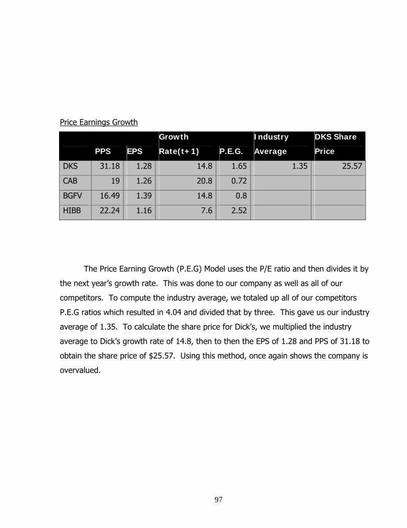
97

Price Earnings Growth

PPS EPS

Growth

Rate(t+1) P.E.G.

Industry

Average

DKS Share

Price

DKS 31.18 1.28 14.8 1.65 1.35 25.57

CAB 19 1.26 20.8 0.72

BGFV 16.49 1.39 14.8 0.8

HIBB 22.24 1.16 7.6 2.52

The Price Earning Growth (P.E.G) Model uses the P/E ratio and then divides it by

the next year’s growth rate. This was done to our company as well as all of our

competitors. To compute the industry average, we totaled up all of our competitors

P.E.G ratios which resulted in 4.04 and divided that by three. This gave us our industry

average of 1.35. To calculate the share price for Dick’s, we multiplied the industry

average to Dick’s growth rate of 14.8, then to then the EPS of 1.28 and PPS of 31.18 to

obtain the share price of $25.57. Using this method, once again shows the company is

overvalued.

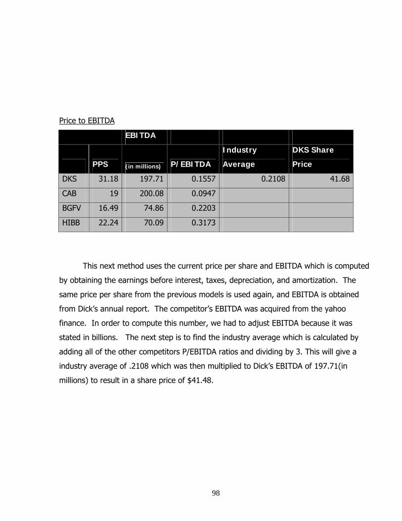
98

Price to EBITDA

EBITDA

PPS (in millions) P/EBITDA

Industry

Average

DKS Share

Price

DKS 31.18 197.71 0.1557 0.2108 41.68

CAB 19 200.08 0.0947

BGFV 16.49 74.86 0.2203

HIBB 22.24 70.09 0.3173

This next method uses the current price per share and EBITDA which is computed

by obtaining the earnings before interest, taxes, depreciation, and amortization. The

same price per share from the previous models is used again, and EBITDA is obtained

from Dick’s annual report. The competitor’s EBITDA was acquired from the yahoo

finance. In order to compute this number, we had to adjust EBITDA because it was

stated in billions. The next step is to find the industry average which is calculated by

adding all of the other competitors P/EBITDA ratios and dividing by 3. This will give a

industry average of .2108 which was then multiplied to Dick’s EBITDA of 197.71(in

millions) to result in a share price of $41.48.

99

Price to FCF per share

PPS FCF (PS) P/FCF (PS)

Industry

Average

DKS Share

Price

DKS 31.18 1.523 20.47 24.226 36.89

CAB 19 -1.363 -13.94

BGFV 16.49 1.186 13.9

HIBB 22.24 0.3058 72.72

The Price to Free Cash Flow is another ratio used to calculate the estimated price

per share for the company. This ratio is computed by dividing the current price per share

by the free cash flows of the company. The same price per share for each company as

before was used again. To find the free cash flow of the company, we used the formula

of FCF = CFFO + (-) CFFI. In other words its cash flows from operating activities plus or

minus the cash flows investing activities. Then to put the free cash flows simply divide it

by the shares outstanding for that year. We calculated the FCF per share for the

competitors off of yahoo finance. The same methodology was computed to find the

industry average which totaled 24.226. To find the price per share for the company,

simply multiply the average by Dick’s PPS of $31.18 and this averaged out to be $36.89.

Up to now this method, has been the only one to undervalue the company. But with this

method the FCF have problems because it tends to fluctuate year by year. This method is

not one of the best ones to use when evaluating a company’s share price.

100

Enterprise Value to EBITDA

EV EBITDA EV/EBITDA

Industry

Average

DKS Share

Price

DKS 2.75 197.71 0.0139 0.0374 14.51

CAB 3.24 200.08 0.0163

BGFV 1.12 74.86 0.0149

HIBB 5.65 70.09 0.0806

This method consists of finding the enterprise value of the company and divide by

the EBITDA. The enterprise value (EV) of company is determined by taking the market

value of equity or (PPS) plus its book value of liabilities minus its cash and cash

equivalents. The EV reported on their annual reports gave us 2.75. The EBITDA as

before is just the earnings before interests, taxes, depreciation, and amortization which

was also included in the annual reports. As for the competitors, we used yahoo finance

to compute the EV and EBITDA. After finding the ratios, we followed the same steps in

calculating the industry average. Again, the EV and the EBITDA were numbers were

adjusted to compute the price per share because the numbers were too high. Then we

took the industry average and multiplied it by the EBITDA, then subtracted the book

value of liabilities and added back the cash and cash equivalents. Finally, we took that

total and divided by the shares outstanding which resulted in a share price of 14.51.

Comparing to the current price of Dick’s to be at 31.18, the company is overvalued.

Conclusion

The method of comparables is another tool that analysts use to determine the value of

the firm. In determining the price per share for Dick’s Sporting Goods, we noticed that

these methods overvalued our most of the time. The only one that we found to

101

undervalue the company was the price to FCF (PS) approach. The closet results that

came near our current share price were the price to book model. Although these

methods do develop a estimate share price, we feel that it might not be the best

approach in valuing the company. It does give of a good benchmark of what to expect

and what variables to use, but the results as a whole were not completely reliable since it

did not produce a share price similar to our current one. Although the results were not

the best, there are other models that do a better estimation in valuating a company.

Intrinsic Models

The intrinsic valuation methods are generally used as a more realistic estimation of

a firm than the comparables method. By using theoretical principles these models are

used to estimate the value of the firm. The methods we used were the Discounted Free

Cash Flow model (FCF), Residual Income model (RI), Long-run Residual Income (LRRI)

model, and the Abnormal Earnings Growth (AEG) model. Below we will discuss each of

these models and how they were used to value Dick’s Sporting Goods. Because Dick’s

Sporting Goods uses operating leases instead of capital leases for their stores, we did not

adjust any of the models using our adjusted balance sheet.

Discount Dividend Model

The discount dividend model values a firm based on the dividends of the firm and

future payouts of dividends. In order to compute the discount dividend model simply use

the forecasted financial value of dividends and the cost of equity. This is a very

unreliable way of calculating the value of the firm, since dividends do not increase

consistently. Dick’s Sporting Goods does not payout dividends, so the discount dividend

model does not apply to them.

Free Cash Flows Model

The Free Cash Flow model estimates the company’s value by using future cash

flow estimations of the company. This model is a comparison between the costs of

capital to growth rate on the perpetuity. Calculating the Free Cash Flow model requires

forecasted cash flows from operations and investments, the calculated before tax WAAC,

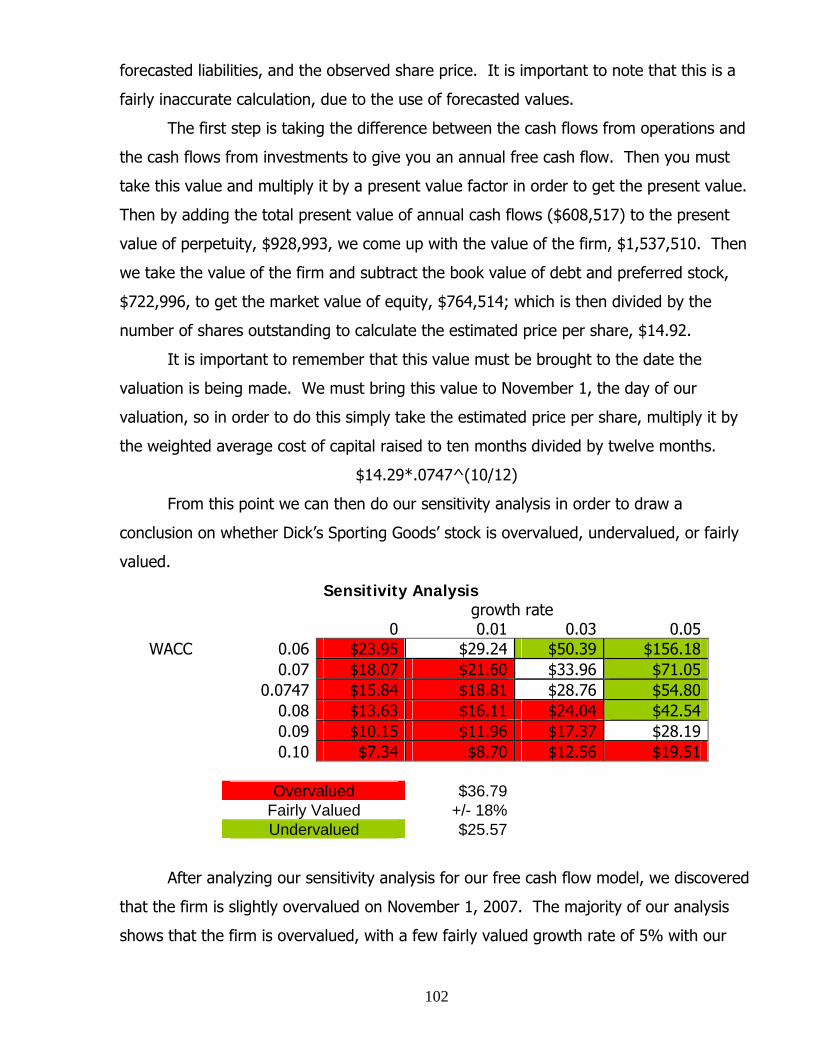
102

forecasted liabilities, and the observed share price. It is important to note that this is a

fairly inaccurate calculation, due to the use of forecasted values.

The first step is taking the difference between the cash flows from operations and

the cash flows from investments to give you an annual free cash flow. Then you must

take this value and multiply it by a present value factor in order to get the present value.

Then by adding the total present value of annual cash flows ($608,517) to the present

value of perpetuity, $928,993, we come up with the value of the firm, $1,537,510. Then

we take the value of the firm and subtract the book value of debt and preferred stock,

$722,996, to get the market value of equity, $764,514; which is then divided by the

number of shares outstanding to calculate the estimated price per share, $14.92.

It is important to remember that this value must be brought to the date the

valuation is being made. We must bring this value to November 1, the day of our

valuation, so in order to do this simply take the estimated price per share, multiply it by

the weighted average cost of capital raised to ten months divided by twelve months.

$14.29*.0747^(10/12)

From this point we can then do our sensitivity analysis in order to draw a

conclusion on whether Dick’s Sporting Goods’ stock is overvalued, undervalued, or fairly

valued.

Sensitivity Analysis growth rate 0 0.01 0.03 0.05

WACC 0.06 $23.95 $29.24 $50.39 $156.18 0.07 $18.07 $21.60 $33.96 $71.05 0.0747 $15.84 $18.81 $28.76 $54.80 0.08 $13.63 $16.11 $24.04 $42.54 0.09 $10.15 $11.96 $17.37 $28.19 0.10 $7.34 $8.70 $12.56 $19.51 Overvalued $36.79 Fairly Valued +/- 18% Undervalued $25.57

After analyzing our sensitivity analysis for our free cash flow model, we discovered

that the firm is slightly overvalued on November 1, 2007. The majority of our analysis

shows that the firm is overvalued, with a few fairly valued growth rate of 5% with our

103

calculated Ke. However we still feel that because the Free Cash Flow model is so

sensitive to changes in Ke, Dick’s Sporting Goods is overvalued.

Residual Income Model

The residual income model is one of the most reliable models from all the

valuation models. This model is based on accounting data and measurements. This

model is not as sensitive as the free cash flow model. This model uses the cost of equity

to discount back to present values. For this model, we had to first come up with the

book value of equity from our previous year and add it to the net income to get the

ending value of equity for each year we were calculating. Dick’s did not have any

dividends so we did not have to subtract any dividends. Normal income was the next

calculation. We calculated it by multiplying beginning book value of equity by the cost of

capital. We then calculated the residual income and subtracted the normal income and

then were able to get the perpetuity from the tenth year of the residual income. After

this, we had to account for the present value and discount it back. These present values

are good indicators to see if a company is adding or destroying value.

0 1 2 3 4 5 6 7 8 9 10

2006 2007 2008 2009 2010 2011201

2201

3 2014 2015 2016PV of

RI 4975

2 3840

1 2865

3 2031

2 1320

3 717

2 208

4 (2182

) (5732

)(8659

)

For our sensitivity analysis we used negative growth rates to bring the price back

to zero. The higher the negative growth rate the change in price rises. Our cost of

equity is 12.096% so we used a couple percents lower and higher of the cost of equity

for the sensitivity analysis. The higher the cost of equity we used, the price would

decrease. The lower the cost of equity, the higher the price we came up with. Even with

these changes, though, our prices stayed fairly consistent. Since our observed price was

$31.18, we assumed 18% was an accurate estimate for our overvalued and undervalued.

So anything under $25.57 is undervalued and anything over $36.79 is overvalued.

Anything that fall in between would be fairly valued.

104

Sensitivity Analysis Growth rate -0.1 -0.2 -0.3 -0.4

Ke 0.1 $10.69 $11.11 $11.33 $11.45 0.12 $10.77 $11.20 $11.41 $11.54 0.12096 $10.98 $11.34 $11.54 $11.66 0.13 $10.22 $10.56 $10.74 $10.85 0.16 $8.10 $8.36 $8.49 $8.58 Over-valued $36.79 Fairly Valued +/- 18% Under-Valued $25.57

In our sensitivity analysis, all of our values were undervalued of the observed price

with that 18% cushion. This analysis demonstrates that Dick’s Sporting Goods is way

overvalued. To even get close to the observed share price of November 1, 2007, Dick’s

would have to have a very low cost of equity. With this in mind, we determined Dick’s is

an overvalued firm.

Long-run Residual Income Model

The long run residual income model uses the original residual income model, and

applies the perpetuity equation that is calculated within the original RI model. This

model uses the calculated Ke, Return on Equity, and the growth rate.

Using our forecasted earnings and book value we can then find our long run return

on equity. We do this by taking our total net income and dividing by the total book value

of equity. Below we present our calculated ROE for each year:

ROE 25.54% 21.36% 18.48% 16.38% 14.78% 13.52% 12.50% 11.67% 10.97% 10.38%

After this step we found the long-run growth of the return on equity. This is a

relatively simply calculation which takes the percent change in book value of equity from

year to year.

Growth % of BVE -16.4% -13.5% -11.4% -9.8% -8.5% -7.5% -6.7% -6.0% -5.4%

After this we simply used this equation:

105

Value of Firm= BVE(1+((ROE – Ke/ (Ke-g)

Then we simply took this number and divided by shares outstanding to find the

value of our price per share, $11.85. After this we ran our sensitivity analysis to come up

with an idea of whether Dick’s Sporting Goods was overvalued, undervalued, or fairly

valued according to the long-run residual model.

ROE=.18 Growth Ke 0.05 0.06 0.07 0.08 0.09

0.1 $21.04 $24.28 $29.67 $40.46 $72.830.11 $17.53 $19.42 $22.25 $26.98 $36.42

0.12096 $14.83 $15.93 $17.47 $19.76 $23.520.14 $11.69 $12.14 $12.72 $13.49 $14.570.16 $9.56 $9.71 $9.89 $10.12 $10.40

Growth=.08 ROE Ke 0.14 0.16 0.18 0.2 0.22

0.1 $24.28 $32.37 $40.46 $48.56 $56.650.11 $16.19 $21.58 $26.98 $32.37 $37.77

0.12096 $11.85 $15.81 $19.76 $23.71 $27.660.14 $8.09 $10.79 $13.49 $16.19 $18.880.16 $6.07 $8.09 $10.12 $12.14 $14.16

Ke=.12096 ROE Growth 0.14 0.16 0.18 0.2 0.22

0.05 $10.26 $12.54 $14.83 $17.11 $19.390.06 $10.62 $13.28 $15.93 $18.59 $21.240.07 $11.12 $14.29 $17.47 $20.64 $23.820.08 $11.85 $15.81 $19.76 $23.71 $27.660.09 $13.07 $18.30 $23.52 $28.75 $33.98

After running the sensitivity analysis and with the calculated price per share of

$11.85, we felt that the firm was overvalued. Even when we manipulated the numbers in

the analysis the only way we could come up with a fair value was with a growth rate of

8% and an ROE of 0.22. While this is not extraordinary we did not feel that it was

realistic, so we believed that the stock was overvalued, if only slightly.

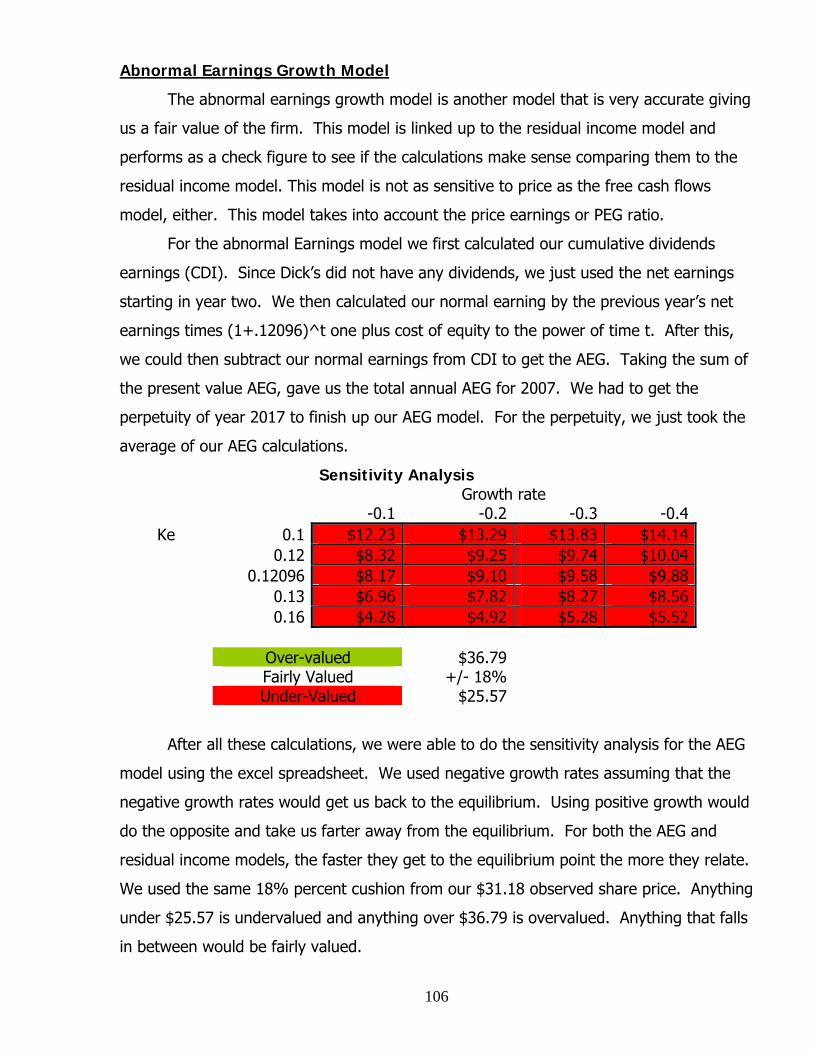
106

Abnormal Earnings Growth Model

The abnormal earnings growth model is another model that is very accurate giving

us a fair value of the firm. This model is linked up to the residual income model and

performs as a check figure to see if the calculations make sense comparing them to the

residual income model. This model is not as sensitive to price as the free cash flows

model, either. This model takes into account the price earnings or PEG ratio.

For the abnormal Earnings model we first calculated our cumulative dividends

earnings (CDI). Since Dick’s did not have any dividends, we just used the net earnings

starting in year two. We then calculated our normal earning by the previous year’s net

earnings times (1+.12096)^t one plus cost of equity to the power of time t. After this,

we could then subtract our normal earnings from CDI to get the AEG. Taking the sum of

the present value AEG, gave us the total annual AEG for 2007. We had to get the

perpetuity of year 2017 to finish up our AEG model. For the perpetuity, we just took the

average of our AEG calculations.

Sensitivity Analysis Growth rate -0.1 -0.2 -0.3 -0.4

Ke 0.1 $12.23 $13.29 $13.83 $14.14 0.12 $8.32 $9.25 $9.74 $10.04 0.12096 $8.17 $9.10 $9.58 $9.88 0.13 $6.96 $7.82 $8.27 $8.56 0.16 $4.28 $4.92 $5.28 $5.52 Over-valued $36.79 Fairly Valued +/- 18% Under-Valued $25.57

After all these calculations, we were able to do the sensitivity analysis for the AEG

model using the excel spreadsheet. We used negative growth rates assuming that the

negative growth rates would get us back to the equilibrium. Using positive growth would

do the opposite and take us farter away from the equilibrium. For both the AEG and

residual income models, the faster they get to the equilibrium point the more they relate.

We used the same 18% percent cushion from our $31.18 observed share price. Anything

under $25.57 is undervalued and anything over $36.79 is overvalued. Anything that falls

in between would be fairly valued.

107

Conclusion

With the abnormal earnings model we get very closely related outcomes because

the residual and AEG models are so closely related. This model also tells us that Dick’s

Sporting Goods is overvalued. As we compared all of our models, we concluded they all

agreed with Dick’s being overvalued. All of these models constructed the same idea of

valuing a firm in their own unique way.

Revised Discounted Free Cash Flows

After accounting for capital leases, we were able to run our Free Cash Flow

analysis to get a different aspect now that we accounted for capital leases. With this

model we saw that Dick’s was undervalued to the actual price of $31.18 at November 1,

2007. The lower we made our WACC the higher, the price we would get. Increasing our

growth rate also increased Dick’s implied share price.

Sensitivity Analysis with Capital Leases

0 0.01 0.03 0.05 WACC 0.06 $54.54 $61.29 $88.28 $223.27

0.07 $46.58 $51.09 $66.86 $124.71 0.0747 $43.53 $47.33 $60.01 $93.24 0.08 $40.48 $43.65 $53.77 $81.60 0.09 $35.63 $37.94 $44.84 $58.66 0.10 $31.66 $33.39 $38.32 $47.19 Over-valued $36.79

Fairly Valued +/- 18%

Under-Valued $25.57 Revised Residual Income Model

After correcting the Residual Income Model, we then got a better measure of

accuracy in valuing Dick’s. Sense this model is one of the best models in terms of

accuracy. We were then able to get a better picture in measuring the value of Dick’s.

The sensitivity we ran gave us all implied price under the observed share price of 31.18.

Just like all of the models that gave us all numbers under this price, simply means that

Dick’s is overvalued. As you can see from our table, the prices don’t even come near the

108

observed price. Accounting for capital leases, did not change the outcome from the

Residual Model.

Sensitivity Analysis with Capital Leases

Sensitivity Analysis Growth rate -0.1 -0.2 -0.3 -0.4

Ke 0.1 $10.87 $11.30 $11.51 $11.64 0.12 $11.15 $11.52 $11.72 $11.83 0.12096 $11.17 $11.53 $11.73 $11.84 0.13 $11.29 $11.63 $11.82 $11.93 0.16 $11.67 $11.96 $12.12 $12.22 Over-valued $36.79

Fairly Valued +/- 18%

Under-Valued $25.57

109

Revised AEG Model

After accounting for capital leases and running the correct data into the AEG

model we then saw a little change in our estimated prices. The revised and regular AEG

model’s stayed fairly consistent in the implied prices. This model again proved that Dick’s

is fairly overvalued. We did observe a slim decrease in the implied price from the regular

AEG model. This decrease is because of the corrections made to the financials from the

capital leases.

Sensitivity AEG with capital leases

Sensitivity Analysis Growth rate -0.1 -0.2 -0.3 -0.4

Ke 0.1 $10.70 $11.84 $12.58 $13.02 0.12 $7.02 $8.21 $8.83 $9.22 0.12096 $6.90 $8.07 $8.67 $9.07 0.13 $5.86 $6.93 $7.50 $7.85 0.16 $3.58 $4.34 $4.77 $5.04 Over-valued $36.79 Fairly Valued +/- 18% Under-Valued $25.57

Credit Analysis In order to value the credit worthiness of Dick’s Sporting Goods, we used the

Altman Z-score. This is a measure of the probability that a company will go bankrupt.

The Altman Z-score uses 5 different ratios from balance and income statements to

calculate this measure. When the calculations turn out to be 1.81 or less, simply mean

that the company is a high risk and more than likely will go bankrupt. When the

outcomes are “between” 1.81 to 2.67, the company is in a gray area. Finally when the

company is greater than 3.28 then the company is a grade A investment and is less risk

to go bankrupt. Basically the higher the number the less risk there is to fail.

110

Altman Z-Score

Z-Score = 1.2(Working Capital/Total Assets) + 1.4(Retained Earnings/Total

Assets) + 3.3(Earnings before Interest and Taxes/Total Assets) + .6(Market

Value of Equity/Book Value of Debt) + 1.0(Sales/Total Assets)

In calculating Dick’s Sporting Goods z-score we can conclude that Dick’s is a grade

A investment due to the fact that their scores in 2006 are 3.718. They did seem to go

down in 2005 to 3.148 just a little under 3.28. We concluded this downturn was from the

acquisition of Galyan’s in June 2004. Even with this decrease though, Dick’s never gets

in the gray area and can be easy determined that they are a high credit company. We

can also determine in the past years they have not been at risk of bankruptcy from the

calculations of the Altman Z-score.

Conclusion

The Altman Z-score calculations gave us great insight in the credit analysis for

Dick’s Sporting Goods. The Altman Z-score helped us determined that Dick’s was a grade

A investment and at no risk of bankruptcy in the near future. This credit analysis uses

the 5 different ratios from the balance sheet and income statement to account for this

credit evaluation.

Year (dks) 2002 2003 2004 2005 2006

Z-Score 4.742 5.135 4.996 3.148 3.718

111

Analyst Recommendation

After dedicating so much time and effort with this project we can now give analyst

recommendations of how to value a firm. We now have a much better understanding of

the industry analysis, accounting analysis, financial analysis, forecasting financial

statements, and intrinsic valuation models which give us the knowledge and expertise to

make precise observations in the valuation process.

In the sporting goods industry, the major competitors of Dick’s Sporting Goods are

Big 5 Sporting Goods, Cabela’s Incorporated, and Hibbett Sporting Goods. Due to the

fragmentation companies must rely on merchandising and marketing skills. This industry

is highly competitive and therefore Dick’s key success factors are required to stay on top

of the industry. The bargaining power of supplier and customers play major roles in the

industry. The relationship that already exists between the firms and their costumers

make it extra difficult for new companies to enter into the market.

In the accounting analysis, the financial statements are used to better understand

how well a firm is operating and if the firm is profitable. Accounting distortions can be

manipulated in the way managers disclose information. We evaluated Dick’s Sporting

Goods and all its competitors to get a big picture of how well they present their

information. The flexibility of GAAP to allow different reporting methods allows managers

to cover some of the true values of a company. With Dick’s Sporting Goods we felt that

there was a good amount of information disclosure when dealing with their financials,

and they provided a decent amount of information regarding mergers and their leasing

policy. Financial Analysis gave us insight in determining how well a company is doing

within a certain industry. We used liquidity, profitability, and capital structure ratios and

compared Dick’s ratios within the industry to see how they compared with each other.

Most of the ratios proved Dick’s to be ahead of the industry average. We also used some

of the ratios that had trends to the financials to forecast the financial statements. The

balance sheet showed the most accuracy in terms of confidence and error. The most

recent year’s forecasts will show a better accurate number. The farther away we move

into the future, the more noise and error there is in the estimations.

112

The intrinsic valuations models consisted of the free cash flows, residual income,

long run residual income, and the abnormal earnings model. All of these models gave us

the same outcomes in our valuation of Dick’s Sporting Goods. The PEG ratio indicated

Dick’s estimated share price at $25.57, and therefore indicates that Dick’s is overvalued.

From all of our sensitivity analysis, especially the residual income and AEG models we

conclude that Dick’s is around $15 to 25$ overvalued. Dick’s current market price is

$31.18 and the calculations were under by the 15 to 25. That’s how we determined that

Dick’s is overvalued. As a result of the intrinsic valuations, now that we concluded Dick’s

to be overvalued, we must also conclude Dick’s Sporting Goods (DKS), a sell

recommendation.

113

Appendix

2002 2003 2004 2005 2006 2002 2003 2004 2005 2006DKS 1.41 1.25 1.60 1.32 1.30 DKS 88.28 89.73 207.11 85.75 106.05HIBB 2.80 3.20 3.08 2.73 2.73 HIBB 102.52 82.82 89.23 77.73 92.79BGFV 1.94 1.58 1.61 1.62 1.58 BGFV 73.68 73.62 83.90 110.02 103.04CAB 1.57 1.65 1.61 1.27 1.54 CAB 41.68 42.24 46.05 50.09 46.85Average 1.93 1.92 1.97 1.73 1.79 Average 76.54 72.10 106.57 80.90 87.18

2002 2003 2004 2005 2006 2002 2003 2004 2005 2006DKS 0.14 0.12 0.46 0.12 0.84 DKS 4.13 4.07 1.76 4.26 3.44HIBB 0.21 0.53 1.03 1.05 0.82 HIBB 3.56 4.41 4.09 4.70 3.93BGFV 1.70 1.70 1.87 1.98 1.62 BGFV 4.95 4.96 4.18 3.32 3.54CAB 0.62 0.64 0.62 0.22 0.35 CAB 3.38 3.15 2.96 2.68 2.49Average 0.92 0.91 0.70 1.05 1.23 Average 4.01 4.15 3.25 3.74 3.35

2002 2003 2004 2005 2006 2002 2003 2004 2005 2006DKS 4.64 4.55 5.99 4.12 6.23 DKS 18.45 26.69 15.43 20.45 21.82HIBB 2.06 2.23 2.29 2.48 2.69 HIBB 4.28 3.93 3.30 3.56 4.46BGFV 2.53 2.46 2.43 2.41 2.41 BGFV 9.18 8.66 9.84 10.78 8.74CAB 3.38 3.15 2.96 2.68 2.49 CAB 6.48 6.07 5.62 12.16 6.10Average 3.15 3.10 3.42 2.92 3.46 Average 9.60 11.34 8.55 11.74 10.28

2002 2003 2004 2005 2006DKS 79 80 61 89 59HIBB 177 164 159 147 135BGFV 144 148 150 152 155CAB 108 116 123 136 147Average 102 102 99 105 99

Working Capital Turnover

Inventory Days

Inventory Turnover

A/R DaysQuick Ratio

Current Ratio

Liquidity Ratios

A/R Turnover

114

2002 2003 2004 2005 2006 2002 2003 2004 2005 2006DKS 0.27 0.28 0.28 0.28 0.29 DKS n/a 0.16 0.18 0.13 0.10HIBB 0.31 0.31 0.32 0.32 0.33 HIBB 0.11 0.12 0.15 0.15 0.17BGFV 0.36 0.36 0.36 0.37 0.35 BGFV 0.68 0.09 0.12 0.13 0.09CAB 0.40 0.40 0.40 0.40 0.41 CAB n/a n/a n/a n/a n/aAverage 0.33 0.34 0.34 0.34 0.35 Average 0.40 0.13 0.15 0.14 0.12

2002 2003 2004 2005 2006 2002 2003 2004 2005 2006DKS 0.05 0.06 0.05 0.05 0.06 DKS 4.10 1.68 1.26 2.46 1.86HIBB 0.08 0.08 0.10 0.10 0.12 HIBB 0.36 0.33 0.36 0.55 0.57BGFV 0.07 0.08 0.08 0.08 0.06 BGFV n/a 4.24 3.34 2.35 1.78CAB 0.06 0.06 0.06 0.06 0.07 CAB 1.33 1.54 1.32 1.14 1.38Average 0.07 0.07 0.07 0.08 0.08 Average 1.93 1.95 1.57 1.62 1.40

2002 2003 2004 2005 2006DKS 0.03 0.04 0.03 0.03 0.04 2002 2003 2004 2005 2006HIBB 0.05 0.05 0.06 0.07 0.08 DKS n/a 0.83 0.49 0.30 0.36BGFV 0.03 0.03 0.04 0.04 0.03 HIBB n/a 0.18 0.20 0.20 0.26CAB 0.06 0.06 0.06 0.06 0.07 BGFV n/a 6.38 1.68 0.62 0.51Average 0.04 0.05 0.05 0.05 0.05 CAB n/a 0.20 0.17 0.13 0.13

Average n/a 1.90 0.64 0.31 0.31

2002 2003 2004 2005 2006DKS 3.95 3.91 3.88 2.42 2.62HIBB 2.09 2.15 1.85 1.67 2.48BGFV 2.59 2.52 2.54 2.50 2.31CAB 1.46 1.44 1.26 1.30 1.17Average 2.52 2.51 2.38 1.97 2.14

Profitability Ratios

Return On Equity

Debt to Equity

Return on Assets

Operating Profit Margin

Gross Profit Margin

Net Profit Margin

Asset Turnover

115

Capital Structure

2002 2003 2004 2005 2006DKS 22.19 47.70 14.34 9.39 18.72HIBB 29.58 26.99 21.34 39.90 45.97BGFV -0.24 -0.36 -0.49 -0.62 -0.76CAB n/a n/a n/a n/a n/aAverage 17.18 24.78 11.73 16.22 21.31

2002 2003 2004 2005 2006DKS n/a 0.69 0.79 0.91 0.80HIBB n/a n/a n/a n/a n/aBGFV n/a n/a n/a n/a n/aCAB 1.79 1.51 1.77 2.16 8.47Average 1.79 1.10 1.28 1.54 4.64

2002 2003 2004 2005 2006DKS 4.10 1.68 1.26 2.46 1.86HIBB 0.44 0.33 0.43 0.55 0.57BGFV 11.73 7.69 4.76 3.66CAB 0.02 0.03 0.05 0.18 0.13Average 1.52 3.44 2.36 1.99 1.56

Times Earned Interest

Debt to Equity

Debt Service Margin

116

3-Month Regression

60 Months SUMMARY OUTPUT

Regression Statistics Multiple R 0.432883133 R Square 0.187387807 Adjusted R Square 0.173131453 Standard Error 0.090893004

Observations 59

ANOVA

df SS MS F Significance F Regression 1 0.108590982 0.108590982 13.14416039 0.000616304 Residual 57 0.470907674 0.008261538

Total 58 0.579498657

Coefficients Standard

Error t Stat P-value Lower 95% Upper 95% Lower 95.0% Upper 95.0%

Intercept 0.066096358 0.01430589 4.620220053 2.23596E-05 0.037449309 0.094743408 0.037449309 0.094743408

X Variable 1 1.40983788 0.388868487 3.625487608 0.000616304 0.631142173 2.188533587 0.631142173 2.188533587

42 Months SUMMARY OUTPUT

Regression Statistics

Multiple R 0.392413227 R Square 0.153988141 Adjusted R Square 0.132837844 Standard Error 0.077679577

Observations 42

ANOVA

df SS MS F Significance F Regression 1 0.043932358 0.043932358 7.28066109 0.010158102 Residual 40 0.241364667 0.006034117

Total 41 0.285297025

Coefficients Standard

Error t Stat P-value Lower 95% Upper 95% Lower 95.0% Upper 95.0%

Intercept 0.065139325 0.018856144 3.454541071 0.001318265 0.027029636 0.103249015 0.027029636 0.103249015

X Variable 1 1.34687727 0.499163264 2.698270018 0.010158102 0.338030691 2.35572385 0.338030691 2.35572385

36 Month

117

SUMMARY OUTPUT

Regression Statistics

Multiple R 0.343986267 R Square 0.118326552 Adjusted R Square 0.09239498 Standard Error 0.08142001

Observations 36

ANOVA

df SS MS F Significance F Regression 1 0.030249323 0.030249323 4.563030423 0.039952435 Residual 34 0.225393412 0.006629218

Total 35 0.255642735

Coefficients Standard

Error t Stat P-value Lower 95% Upper 95% Lower 95.0% Upper 95.0%

Intercept 0.061217407 0.022970083 2.665093021 0.011687837 0.014536583 0.107898231 0.014536583 0.107898231

X Variable 1 1.229031221 0.575355453 2.136125095 0.039952435 0.059768268 2.398294174 0.059768268 2.398294174

24 Month SUMMARY OUTPUT

Regression Statistics Multiple R 0.422640525 R Square 0.178625013 Adjusted R Square 0.141289787 Standard Error 0.068800568

Observations 24

ANOVA

df SS MS F Significance F Regression 1 0.022646835 0.022646835 4.78435594 0.039635334 Residual 22 0.104137398 0.004733518

Total 23 0.126784234

Coefficients Standard

Error t Stat P-value Lower 95% Upper 95% Lower 95.0% Upper 95.0%

Intercept 0.090843035 0.028072558 3.236008414 0.003795585 0.032624113 0.149061958 0.032624113 0.149061958

X Variable 1 1.451133061 0.663430595 2.187317064 0.039635334 0.075262224 2.827003897 0.075262224 2.827003897

118

1-Year 60-Month SUMMARY OUTPUT

Regression Statistics

Multiple R 0.445609283

R Square 0.198567633 Adjusted R Square 0.184507416

Standard Error 0.090265591

Observations 59

ANOVA

df SS MS F Significance

F

Regression 1 0.115069677 0.115069677 14.12265785 0.000404981

Residual 57 0.46442898 0.008147877

Total 58 0.579498657

Coefficients Standard

Error t Stat P-value Lower 95% Upper 95% Lower 95.0%

Upper 95.0%

Intercept 0.070983157 0.014836306 4.784422558 1.25329E-05 0.041273967 0.100692348 0.041273967 0.100692348

X Variable 1 1.467653635 0.39053985 3.758012486 0.000404981 0.685611079 2.24969619 0.685611079 2.24969619

48-Month SUMMARY OUTPUT

Regression Statistics

Multiple R 0.32795975

R Square 0.107557598 Adjusted R Square 0.088156676

Standard Error 0.081073153

Observations 48

ANOVA

df SS MS F Significance

F

Regression 1 0.036439538 0.036439538 5.543942645 0.022868753

Residual 46 0.302351386 0.006572856

Total 47 0.338790924

Coefficients Standard

Error t Stat P-value Lower 95% Upper 95% Lower 95.0%

Upper 95.0%

Intercept 0.057607866 0.01763877 3.265979775 0.00206467 0.022102864 0.093112867 0.022102864 0.093112867

X Variable 1 1.100967307 0.467589832 2.354557845 0.022868753 0.159757807 2.042176807 0.159757807 2.042176807

36-Month

119

SUMMARY OUTPUT

Regression Statistics

Multiple R 0.3672172

R Square 0.134848472 Adjusted R Square 0.109402839

Standard Error 0.080653526

Observations 36

ANOVA

df SS MS F Significance

F

Regression 1 0.034473032 0.034473032 5.299474023 0.02758355

Residual 34 0.221169703 0.006504991

Total 35 0.255642735

Coefficients Standard

Error t Stat P-value Lower 95% Upper 95% Lower 95.0%

Upper 95.0%

Intercept 0.067091018 0.02388951 2.808388239 0.008191018 0.018541693 0.115640343 0.018541693 0.115640343

X Variable 1 1.331353003 0.578331488 2.302058649 0.02758355 0.156042019 2.506663987 0.156042019 2.506663987

24-Month SUMMARY OUTPUT

Regression Statistics

Multiple R 0.423576345

R Square 0.17941692 Adjusted R Square 0.14211769

Standard Error 0.068767393

Observations 24

ANOVA

df SS MS F Significance

F

Regression 1 0.022747237 0.022747237 4.81020429 0.039153682

Residual 22 0.104036997 0.004728954

Total 23 0.126784234

Coefficients Standard

Error t Stat P-value Lower 95% Upper 95% Lower 95.0%

Upper 95.0%

Intercept 0.092246933 0.028568302 3.228995957 0.003858959 0.0329999 0.151493966 0.0329999 0.151493966

X Variable 1 1.4561649 0.663939945 2.193217794 0.039153682 0.079237737 2.833092064 0.079237737 2.833092064

120

2-Year 60-Month SUMMARY OUTPUT

Regression Statistics

Multiple R 0.457505792

R Square 0.20931155 Adjusted R Square 0.195439823

Standard Error 0.089658504

Observations 59

ANOVA

df SS MS F Significance

F

Regression 1 0.121295762 0.121295762 15.08907628 0.000269412

Residual 57 0.458202895 0.008038647

Total 58 0.579498657

Coefficients Standard

Error t Stat P-value Lower 95% Upper 95% Lower 95.0%

Upper 95.0%

Intercept 0.075983522 0.015402128 4.933313194 7.36887E-06 0.045141293 0.106825751 0.045141293 0.106825751

X Variable 1 1.558760636 0.401280543 3.884466022 0.000269412 0.755210215 2.362311058 0.755210215 2.362311058

48-Months SUMMARY OUTPUT

Regression Statistics

Multiple R 0.345586695

R Square 0.119430164 Adjusted R Square 0.100287341

Standard Error 0.080532071

Observations 48

ANOVA

df SS MS F Significance

F

Regression 1 0.040461856 0.040461856 6.23890044 0.016136048

Residual 46 0.298329068 0.006485415

Total 47 0.338790924

Coefficients Standard

Error t Stat P-value Lower 95% Upper 95% Lower 95.0%

Upper 95.0%

Intercept 0.062455186 0.018492054 3.3774066 0.001497302 0.025232612 0.09967776 0.025232612 0.09967776

X Variable 1 1.211705404 0.485113116 2.497779102 0.016136048 0.235223362 2.188187445 0.235223362 2.188187445

36-Months SUMMARY OUTPUT

121

Regression Statistics

Multiple R 0.389665919

R Square 0.151839529 Adjusted R Square 0.126893632

Standard Error 0.079857605

Observations 36

ANOVA

df SS MS F Significance

F

Regression 1 0.038816672 0.038816672 6.086753797 0.018814181

Residual 34 0.216826063 0.006377237

Total 35 0.255642735

Coefficients Standard

Error t Stat P-value Lower 95% Upper 95% Lower 95.0%

Upper 95.0%

Intercept 0.070578401 0.023891586 2.954111142 0.005656474 0.022024856 0.119131945 0.022024856 0.119131945

X Variable 1 1.428829779 0.579145419 2.467134734 0.018814181 0.251864688 2.605794869 0.251864688 2.605794869

24-Month SUMMARY OUTPUT

Regression Statistics

Multiple R 0.42050963

R Square 0.176828349 Adjusted R Square 0.139411456

Standard Error 0.068875773

Observations 24

ANOVA

df SS MS F Significance

F

Regression 1 0.022419047 0.022419047 4.725896088 0.04074951

Residual 22 0.104365187 0.004743872

Total 23 0.126784234

Coefficients Standard

Error t Stat P-value Lower 95% Upper 95% Lower 95.0%

Upper 95.0%

Intercept 0.089564469 0.027701737 3.233171586 0.0038211 0.032114583 0.147014355 0.032114583 0.147014355

X Variable 1 1.431374987 0.658432622 2.173912622 0.04074951 0.065869312 2.796880662 0.065869312 2.796880662

122

5-Year 60-Month SUMMARY OUTPUT

Regression Statistics

Multiple R 0.457605463

R Square 0.20940276 Adjusted R Square 0.195532633

Standard Error 0.089653332

Observations 59

ANOVA

df SS MS F Significance

F

Regression 1 0.121348618 0.121348618 15.09739309 0.000268477

Residual 57 0.458150039 0.00803772

Total 58 0.579498657

Coefficients Standard

Error t Stat P-value Lower 95% Upper 95% Lower 95.0%

Upper 95.0%

Intercept 0.087847496 0.017544954 5.006994971 5.65434E-06 0.052714332 0.12298066 0.052714332 0.12298066

X Variable 1 1.678430628 0.431968834 3.885536397 0.000268477 0.813427965 2.543433292 0.813427965 2.543433292

48-Month SUMMARY OUTPUT

Regression Statistics

Multiple R 0.358562283

R Square 0.128566911 Adjusted R Square 0.109622713

Standard Error 0.080113184

Observations 48

ANOVA

df SS MS F Significance

F

Regression 1 0.043557302 0.043557302 6.786611574 0.01233059

Residual 46 0.295233621 0.006418122

Total 47 0.338790924

Coefficients Standard

Error t Stat P-value Lower 95% Upper 95% Lower 95.0%

Upper 95.0%

Intercept 0.071098039 0.020648612 3.443235829 0.001235434 0.02953454 0.112661538 0.02953454 0.112661538

X Variable 1 1.343491838 0.515713542 2.605112584 0.01233059 0.305414335 2.38156934 0.305414335 2.38156934

36-Month SUMMARY OUTPUT

123

Regression Statistics

Multiple R 0.411132591

R Square 0.169030007 Adjusted R Square 0.144589713

Standard Error 0.079044188

Observations 36

ANOVA

df SS MS F Significance

F

Regression 1 0.043211293 0.043211293 6.916038228 0.012738771

Residual 34 0.212431442 0.006247984

Total 35 0.255642735

Coefficients Standard

Error t Stat P-value Lower 95% Upper 95% Lower 95.0%

Upper 95.0%

Intercept 0.075342584 0.024305063 3.099872065 0.003874071 0.025948755 0.124736414 0.025948755 0.124736414

X Variable 1 1.532116311 0.582590024 2.62983616 0.012738771 0.348150941 2.716081681 0.348150941 2.716081681

24-Month SUMMARY OUTPUT

Regression Statistics

Multiple R 0.417328063

R Square 0.174162712 Adjusted R Square 0.136624653

Standard Error 0.068987202

Observations 24

ANOVA

df SS MS F Significance

F

Regression 1 0.022081086 0.022081086 4.639630252 0.042458798

Residual 22 0.104703148 0.004759234

Total 23 0.126784234

Coefficients Standard

Error t Stat P-value Lower 95% Upper 95% Lower 95.0%

Upper 95.0%

Intercept 0.088719041 0.027565615 3.218467696 0.00395604 0.031551455 0.145886626 0.031551455 0.145886626

X Variable 1 1.419638735 0.659076998 2.153980096 0.042458798 0.052796706 2.786480764 0.052796706 2.786480764

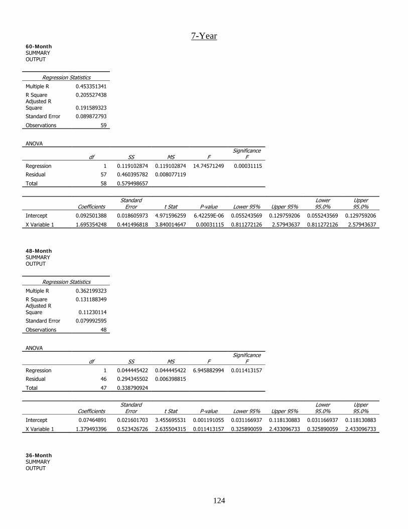
124

7-Year 60-Month SUMMARY OUTPUT

Regression Statistics

Multiple R 0.453351341

R Square 0.205527438 Adjusted R Square 0.191589323

Standard Error 0.089872793

Observations 59

ANOVA

df SS MS F Significance

F

Regression 1 0.119102874 0.119102874 14.74571249 0.00031115

Residual 57 0.460395782 0.008077119

Total 58 0.579498657

Coefficients Standard

Error t Stat P-value Lower 95% Upper 95% Lower 95.0%

Upper 95.0%

Intercept 0.092501388 0.018605973 4.971596259 6.42259E-06 0.055243569 0.129759206 0.055243569 0.129759206

X Variable 1 1.695354248 0.441496818 3.840014647 0.00031115 0.811272126 2.57943637 0.811272126 2.57943637

48-Month SUMMARY OUTPUT

Regression Statistics

Multiple R 0.362199323

R Square 0.131188349 Adjusted R Square 0.11230114

Standard Error 0.079992595

Observations 48

ANOVA

df SS MS F Significance

F

Regression 1 0.044445422 0.044445422 6.945882994 0.011413157

Residual 46 0.294345502 0.006398815

Total 47 0.338790924

Coefficients Standard

Error t Stat P-value Lower 95% Upper 95% Lower 95.0%

Upper 95.0%

Intercept 0.07464891 0.021601703 3.455695531 0.001191055 0.031166937 0.118130883 0.031166937 0.118130883

X Variable 1 1.379493396 0.523426726 2.635504315 0.011413157 0.325890059 2.433096733 0.325890059 2.433096733

36-Month SUMMARY OUTPUT

125

Regression Statistics

Multiple R 0.421372807

R Square 0.177555043 Adjusted R Square 0.153365485

Standard Error 0.07863768

Observations 36

ANOVA

df SS MS F Significance

F

Regression 1 0.045390657 0.045390657 7.340152551 0.010484355

Residual 34 0.210252079 0.006183885

Total 35 0.255642735

Coefficients Standard

Error t Stat P-value Lower 95% Upper 95% Lower 95.0%

Upper 95.0%

Intercept 0.078288207 0.02468085 3.172022274 0.003203118 0.028130685 0.128445729 0.028130685 0.128445729

X Variable 1 1.58388353 0.584616004 2.70927159 0.010484355 0.395800873 2.771966187 0.395800873 2.771966187

24-Month SUMMARY OUTPUT

Regression Statistics

Multiple R 0.417511238

R Square 0.174315634 Adjusted R Square 0.136784526

Standard Error 0.068980814

Observations 24

ANOVA

df SS MS F Significance

F

Regression 1 0.022100474 0.022100474 4.644564075 0.042358883

Residual 22 0.10468376 0.004758353

Total 23 0.126784234

Coefficients Standard

Error t Stat P-value Lower 95% Upper 95% Lower 95.0%

Upper 95.0%

Intercept 0.089297128 0.027785034 3.213857081 0.003999296 0.031674495 0.146919761 0.031674495 0.146919761

X Variable 1 1.42465528 0.661054571 2.155125072 0.042358883 0.053712015 2.795598544 0.053712015 2.795598544

126

10-Year 60-Month SUMMARY OUTPUT

Regression Statistics

Multiple R 0.446928832

R Square 0.199745381 Adjusted R Square 0.185705826

Standard Error 0.090199241

Observations 59

ANOVA

df SS MS F Significance

F

Regression 1 0.11575218 0.11575218 14.22733021 0.000387362

Residual 57 0.463746477 0.008135903

Total 58 0.579498657

Coefficients Standard

Error t Stat P-value Lower 95% Upper 95% Lower 95.0%

Upper 95.0%

Intercept 0.096593866 0.019696193 4.904189759 8.17913E-06 0.057152921 0.136034811 0.057152921 0.136034811

X Variable 1 1.696189634 0.44968945 3.771913336 0.000387362 0.795702049 2.596677218 0.795702049 2.596677218

48-Month SUMMARY OUTPUT

Regression Statistics

Multiple R 0.36189014

R Square 0.130964473 Adjusted R Square 0.112072397

Standard Error 0.080002901

Observations 48

ANOVA

df SS MS F Significance

F

Regression 1 0.044369575 0.044369575 6.932243367 0.0114888

Residual 46 0.294421349 0.006400464

Total 47 0.338790924

Coefficients Standard

Error t Stat P-value Lower 95% Upper 95% Lower 95.0%

Upper 95.0%

Intercept 0.077636373 0.022585025 3.437515442 0.001256333 0.032175076 0.12309767 0.032175076 0.12309767

X Variable 1 1.391979054 0.528683553 2.632915374 0.0114888 0.327794274 2.456163833 0.327794274 2.456163833

36-Month SUMMARY OUTPUT

127

Regression Statistics

Multiple R 0.428296096

R Square 0.183437546 Adjusted R Square 0.159421003

Standard Error 0.078355949

Observations 36

ANOVA

df SS MS F Significance

F

Regression 1 0.046894476 0.046894476 7.637966373 0.009160302

Residual 34 0.208748259 0.006139655

Total 35 0.255642735

Coefficients Standard

Error t Stat P-value Lower 95% Upper 95% Lower 95.0%

Upper 95.0%

Intercept 0.081316054 0.02523856 3.221897583 0.002805597 0.03002513 0.132606978 0.03002513 0.132606978

X Variable 1 1.62351856 0.58744659 2.763687097 0.009160302 0.429683461 2.81735366 0.429683461 2.81735366

24-Month SUMMARY OUTPUT

Regression Statistics

Multiple R 0.418122793

R Square 0.17482667 Adjusted R Square 0.137318791

Standard Error 0.068959464

Observations 24

ANOVA

df SS MS F Significance

F

Regression 1 0.022165265 0.022165265 4.661065259 0.042026644

Residual 22 0.104618968 0.004755408

Total 23 0.126784234

Coefficients Standard

Error t Stat P-value Lower 95% Upper 95% Lower 95.0%

Upper 95.0%

Intercept 0.090464385 0.028213497 3.206422248 0.004070016 0.031953173 0.148975597 0.031953173 0.148975597

X Variable 1 1.433462511 0.6639628 2.158950036 0.042026644 0.056487948 2.810437073 0.056487948 2.810437073

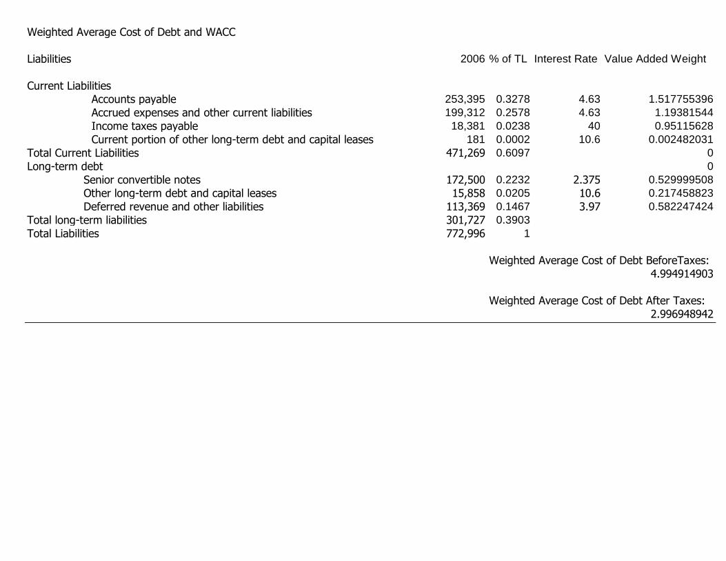
Weighted Average Cost of Debt and WACC

Liabilities 2006 % of TL Interest Rate Value Added Weight

Current LiabilitiesAccounts payable 253,395 0.3278 4.63 1.517755396Accrued expenses and other current liabilities 199,312 0.2578 4.63 1.19381544Income taxes payable 18,381 0.0238 40 0.95115628Current portion of other long-term debt and capital leases 181 0.0002 10.6 0.002482031

Total Current Liabilities 471,269 0.6097 0Long-term debt 0

Senior convertible notes 172,500 0.2232 2.375 0.529999508Other long-term debt and capital leases 15,858 0.0205 10.6 0.217458823Deferred revenue and other liabilities 113,369 0.1467 3.97 0.582247424

Total long-term liabilities 301,727 0.3903Total Liabilities 772,996 1

Weighted Average Cost of Debt BeforeTaxes:4.994914903

Weighted Average Cost of Debt After Taxes:2.996948942

129

Dick's Sporting Goods, Inc. 2006 10-k

Forcasted Income Statement (Revised)

Fiscal Year 2001 2002 2003 2004 2005 2006 Assume Average 2007 2008 2009 2010 2011 2012 2013 2014 2015 2016

(Dollars in thousands, except per share)

Statement of Income Data: 0.05

Net sales $893,396 $1,272,584 $1,470,845 $2,109,399 $2,624,987 $3,114,162 5.00% 100.00% $3,269,870 $3,433,364 $3,605,032 $3,785,283 $3,974,548 $4,173,275 $4,381,939 $4,601,036 $4,831,087 $5,072,642

Cost of goods sold (1) $684,552 $934,956 $1,062,820 $1,522,873 $1,887,347 $2,217,463 72.21% $2,361,173 $2,479,232 $2,603,193 $2,733,353 $2,870,021 $3,013,522 $3,164,198 $3,322,408 $3,488,528 $3,662,955

Gross profit $208,844 $337,628 $408,025 $586,526 $737,640 $896,699 27.79% $908,697 $954,132 $1,001,838 $1,051,930 $1,104,527 $1,159,753 $1,217,741 $1,278,628 $1,342,559 $1,409,687

Selling, general and administrative expenses $169,392 $262,755 $314,885 $443,776 $556,320 $682,625 21.24% $694,520 $729,246 $765,709 $803,994 $844,194 $886,404 $930,724 $977,260 $1,026,123 $1,077,429

Adding Back Operating Lease expenses $74,918 $88,183 $97,100 $144,000 $196,300 $205,800 $230,830 $236,681 $235,771 $235,007 $228,976 $160,283 $112,198 $78,539 $54,977 $38,484

Less capital lease depreciation $12,082 $14,420 $17,554 $37,621 $49,861 $54,929 $60,512 $60,512 $60,512 $60,512 $60,512 $60,512 $60,512 $60,512 $60,512 $60,512

Income from operations $102,288 $148,636 $172,686 $249,129 $327,759 $364,945 5.58% $384,494 $401,054 $411,388 $422,431 $428,797 $373,121 $338,703 $319,394 $310,901 $310,230

Capital Lease Interest Expense $94,241 $144,196 $169,025 $238,479 $311,326 $351,052 $207,594 $215,309 $216,356 $217,647 $213,774 $147,346 $101,640 $70,478 $49,539 $35,800

Interest expense, net $6,963 $2,864 $1,831 $8,009 $12,959 $10,025 0.31% $10,137 $10,643 $11,176 $11,734 $12,321 $12,937 $13,584 $14,263 $14,976 $15,725

Other income (1,000)

Income before income taxes $1,084 $1,576 $1,830 $2,641 $3,474 $3,868 5.41% $176,900 $185,745 $195,032 $204,784 $215,023 $225,774 $237,063 $248,916 $261,362 $274,430

Provision for income taxes $434 $630 $732 $1,056 $1,390 $1,547 2.16% $70,760 $74,298 $78,013 $81,914 $86,009 $90,310 $94,825 $99,566 $104,545 $109,772

Net income with Leases Capitilized $651 $945 $1,098 $1,584 $2,085 $2,321 3.24% $105,944 $111,241 $116,803 $122,643 $128,775 $135,214 $141,975 $149,074 $156,527 $164,354

Net income with Operating Leases 8,643 38,137 52,408 68,905 72,980 112,611 3.24 $116,260 $120,026 $123,915 $127,930 $132,075 $136,354 $140,772 $145,333 $150,042 $154,903

Difference in Net Income due to Capitalization ($7,992) ($37,192) ($51,310) ($67,321) ($70,895) ($110,290) ($10,316) ($8,785) ($7,112) ($5,287) ($3,300) ($1,140) $1,203 $3,740 $6,485 $9,450

Common Size Income Statement (Revised)

Assume Average

Fiscal Year 2002 2003 2004 2005 2006 2007 2008 2009 2010 2011 2012 2013 2014 2015 2016

(Dollars in thousands, except per share and sales per square foot data)

Statement of Income Data:

Sales Growth Percent

Net sales 100% 100% 100% 100% 100% 100% 100% 100% 100% 100% 100% 100% 100% 100% 100%

Cost of goods sold (1) 73.47% 72.26% 72.19% 71.90% 71.21% 72.21% 72.21% 72.21% 72.21% 72.21% 72.21% 72.21% 72.21% 72.21% 72.21% 72.21%

Gross profit 26.53% 27.74% 27.81% 28.10% 28.79% 27.79% 27.79% 27.79% 27.79% 27.79% 27.79% 27.79% 27.79% 27.79% 27.79% 27.79%

Selling, general and administrative expenses 20.65% 21.41% 21.04% 21.19% 21.92% 21.24% 21.24% 21.24% 21.24% 21.24% 21.24% 21.24% 21.24% 21.24% 21.24% 21.24%

Merger integration and store closing costs 6.83% 7.48%

Income from operations 11.68% 11.74% 11.81% 12.49% 11.72% 11.89% 11.76% 11.68% 11.41% 11.16% 10.79% 8.94% 7.73% 6.94% 6.44% 6.12%

investment (2) (3)

Interest expense, net 0.23% 0.12% 0.38% 0.49% 0.32% 0.31% 0.31% 0.31% 0.31% 0.31% 0.31% 0.31% 0.31% 0.31% 0.31% 0.31%

Other income

Income before income taxes 0.12% 0.12% 0.13% 0.13% 0.12% 0.13% 5.41% 5.41% 5.41% 5.41% 5.41% 5.41% 5.41% 5.41% 5.41% 5.41%

Provision for income taxes 0.05% 0.05% 0.05% 0.05% 0.05% 0.05% 2.16% 2.16% 2.16% 2.16% 2.16% 2.16% 2.16% 2.16% 2.16% 2.16%

Net income 0.07% 0.07% 0.08% 0.08% 0.07% 0.08% 3.24% 3.24% 3.24% 3.24% 3.24% 3.24% 3.24% 3.24% 3.24% 3.24%

Actual Financials Forecast Financial Statements

Forecast Financial Statements

130

Forcasted Balance Sheet (Revised) Forecast Financial Statements

2002 2003 2004 2005 2006 Average Assume 2007 2008 2009 2010 2011 2012 2013 2014 2015 2016

ASSETS

CURRENT ASSETS:

Cash and cash equivalents 8,976 11,120 93,674 18,886 365,464

Accounts receivable, net 14,416 16,391 10,185 30,611 29,365 3.2 3.2 30,305 31,274 32,275 33,308 34,374 35,474 36,609 37,780 38,989 40,237

Income tax receivable 232 7,202

Inventories, net 201,585 233,497 254,360 457,618 355,698 5.1 5.1 373,839 392,904 412,942 434,003 456,137 479,400 503,849 529,545 556,552 584,936

Prepaid expenses and other current assets 5,219 5,572 5,222 8,772 11,961

Deferred income taxes 5,243 8,697 1,021 7,966 429

Total current assets 235,439 275,277 364,694 531,055 762,917 51.00% 919,542 1,049,117 1,173,246 1,292,767 1,406,768 1,484,718 1,562,347 1,639,925 1,717,706 1,795,927

Capital-lease rights $88,183 $97,100 $144,000 $196,300 $205,800 208,707 193,488 174,271 157,058 138,361 60,163 54,397 49,183 44,469 40,208

PROPERTY AND EQUIPMENT, NET 71,795 80,109 144,402 349,098 370,277

CONSTRUCTION IN PROGRESS - LEASED FACILITIES 10,927 15,233 7,338

GOODWILL 157,245 156,628

OTHER ASSETS:

Deferred income taxes 5,970 7,512 6,099 871 8,959

Investments 5,770 1,950 7,054 3,388 3,197

Other 3,008 11,378 10,184 28,158 27,373

Total other assets 174,726 198,049 322,666 750,293 779,572 883,482 1,007,976 1,127,236 1,242,070 1,351,600 1,426,494 1,501,078 1,575,614 1,650,345 1,725,498

TOTAL ASSETS 410,165 473,326 687,360 1,281,348 1,542,489 3.36% 1,803,024 2,057,093 2,300,482 2,534,836 2,758,368 2,911,212 3,063,425 3,215,540 3,368,051 3,521,425

LIABILITIES AND STOCKHOLDERS' EQUITY

CURRENT LIABILITIES:

Accounts payable 95,573 125,208 118,383 211,685 253,395

Accrued expenses 47,012 59,239 72,090 141,465 136,520

Deferred revenue and other liabilities 17,958 22,752 37,037 48,882 62,792

Income taxes payable 5,728 12,763 18,381

Current portion of other long-term debt 211 213 505 635 181

Total current liabilities 166,482 220,175 228,015 402,667 471,269 1.40% 477,867 484,557 491,341 498,219 505,195 512,267 519,439 526,711 534,085 541,562

LONG-TERM LIABILITIES:

Senior convertible notes 172,500 172,500

Revolving credit borrowings 77,073 76,094 148,900

Capital Lease Obligation $88,183 $97,100 $144,000 $196,300 $205,800 208,707 193,488 174,271 157,058 138,361 60,163 54,397 49,183 44,469 40,208

Other long-term debt 3,577 3,364 3,411 8,775 8,520

Non-cash obligations for construction in progress - leased facilities 10,927 15,233 7,338

Deferred revenue and other liabilities 11,745 12,188 60,113 96,112 113,369

Total long-term liabilities 180,578 112,652 218,451 565,014 656,427

Total Liabilities 347,060 332,827 446,466 967,681 1,127,696 66.98% 1,276,580 1,297,241 1,315,111 1,336,230 1,357,154 1,319,907 1,356,468 1,395,004 1,435,510 1,477,987

COMMITMENTS AND CONTINGENCIES

STOCKHOLDERS' EQUITY:Preferred stock, par value, $.01 per share, authorized shares 5,000,000; none issued and outstandingCommon stock, par value, $.01 per share, authorized shares 200,000,000; issued and outstanding

shares 36,545,332 and 34,790,358, at January 28, 2006 and January 29, 2005, respectively 169 126 331 348 365

Class B common stock, par value, $.01 per share, authorized shares 40,000,000; issued and

outstanding shares 13,730,945 and 14,039,529, at January 28, 2006 and January 29, 2005, respectively 77 141 140 137

Additional paid-in capital 96,279 130,071 175,748 181,321 209,526

Retained earnings 28,029 10,225 60,957 129,862 202,842 114,894 235,750 152,394 271,860 190,623 370,247 217,255 397,028 244,262 424,331

Notes receivables for common stock 6,196

Accumulated other comprehensive income 882 3,717 1,996 1,923

Total stockholders' equity 63,105 140,499 240,894 313,667 414,793 317,736 350,644 388,144 424,254 462,483 560,870 587,502 614,283 641,290 668,593

TOTAL LIABILITIES AND STOCKHOLDERS' EQUITY 410,165 473,326 687,360 1,281,348 1,542,489 3.36% 1,594,317 1,647,886 1,703,255 1,760,484 1,819,636 1,880,776 1,943,970 2,009,287 2,076,800 2,146,580

Actual Financial Statements

131

Discounted Free Cash Flows

2006 2007 2008 2009 2010 2011 2012 2013 2014 2015 2016Cash Flow from Operations 178,007 186,907 196,252 206,065 216,368 227,186 238,546 250,473 262,997 276,147Cash Provided (Used) by Investing Activities ($98,404) ($103,324) ($108,490) ($113,915) ($119,611) ($125,591) ($131,871) ($138,464) ($145,387) ($152,657)Free Cash Flow (to firm) 79,603 83,583 87,762 92,150 96,757 101,595 106,675 112,009 117,609 123,490discount rate (9% WACC) 0.93 0.87 0.81 0.75 0.70 0.65 0.60 0.56 0.52 0.49Present Value of Free Cash Flows $74,070 $72,367 $70,704 $69,079 $67,491 $65,940 $64,425 $62,944 $61,497 $60,084Total Present Value of Annual Cash Flows $608,517Continuing (Terminal) Value (assume no growth) 1653142.697Present Value of Continuing (Terminal) Value $928,993 gValue of the Firm $1,537,510 0 0.01 0.03 0.05Book Value of Debt and Preferred Stock $772,996 WACC 0.06 $23.95 $29.24 $50.39 $156.18Value of Equity $764,514 0.07 $18.07 $21.60 $33.96 $71.05

0.0747 $15.84 $18.81 $28.76 $54.80Estimated Value $14.92 0.08 $13.63 $16.11 $24.04 $42.54Implied Share Price Nov. 1, 2007 $15.84 0.09 $10.15 $11.96 $17.37 $28.19growth 0 0.10 $7.34 $8.70 $12.56 $19.51Actual Price per share $31.18

$36.79 +/- 18%

$25.57

Additional Exercises

d a b c c/ddebt % equity % wacc k_d wacc-dwac

Ke based on WACC 50.28% 49.72% 0.0747 0.04990 0.02480 0.049875137

Fairly ValuedUnder-Valued

Sensitivity Analysis

Over-valued

132

Risidual Income ValuationDifference in RI ($7,518) ($7,894) ($8,288) ($8,703) ($9,138) ($9,595) ($10,075) ($10,578) ($11,107)

1 2 3 4 5 6 7 8 9 10 11Perp

2006 2007 2008 2009 2010 2011 2012 2013 2014 2015 2016 2017Total Book Value Beg 414,793 520,737 631,978 748,781 871,424 1,000,199 1,135,413 1,277,388 1,426,462 1,582,989Total Net Income 105,944 111,241 116,803 122,643 128,775 135,214 141,975 149,074 156,527 164,354Dividends per share 0 0 0 0 0 0 0 0 0 0Ending BE 414,793 520,737 631,978 748,781 871,424 1,000,199 1,135,413 1,277,388 1,426,462 1,582,989 1,747,343Ke 0.12096"Normal" Income 50,173 62,988 76,444 90,573 105,407 120,984 137,340 154,513 172,545 191,478Residual Income (RI) 55,770 48,253 40,359 32,071 23,368 14,230 4,635 -5,439 -16,018 -27,125 -37,967Discount Factor 0.89 0.80 0.71 0.63 0.57 0.50 0.45 0.40 0.36 0.32Present Value of RI 49752 38401 28653 20312 13203 7172 2084 (2182) (5732) (8659)

ROE 0.255 0.214 0.185 0.164 0.148 0.135 0.125 0.117 0.110 0.104BV Equity 2006 414,793 gr -16.4% -13.5% -11.4% -9.8% -8.5% -7.5% -6.7% -6.0% -5.4% 0.156Total PV of RI (end 2006) 151663.89 -171830Continuation (Terminal) Value -54853PV of Terminal Value (end 2006) (54853) g avg gr -9.4%Market Value of equity 2006 $511,604.32 -0.1 -0.2 -0.3 -0.4Shares outstanding 51,256 Ke 0.1 $10.69 $11.11 $11.33 $11.45Price end of 2006 $9.98 0.12 $10.77 $11.20 $11.41 $11.54Time Consistent Implied Price $10.98 0.12096 $10.98 $11.34 $11.54 $11.66Actual Price per share $31.18 0.13 $10.22 $10.56 $10.74 $10.85Growth -0.1 0.16 $8.10 $8.36 $8.49 $8.58Ke 0.12096

$36.79 +/- 18%

$25.57

Over-valuedFairly ValuedUnder-Valued

Forecast Years

Sensitivity Analysis

133

Long-run Risidual Income$36.79

BookEquity 414,793 +/- 18%Ke 0.12096 $25.57ROE 0.22g 0.09

ROE=.18Growth

PPS $33.98 Ke 0.05 0.06 0.07 0.08 0.090.1 $21.04 $24.28 $29.67 $40.46 $72.83

0.11 $17.53 $19.42 $22.25 $26.98 $36.420.12096 $14.83 $15.93 $17.47 $19.76 $23.52

0.14 $11.69 $12.14 $12.72 $13.49 $14.570.16 $9.56 $9.71 $9.89 $10.12 $10.40

Growth=.08ROE

Ke 0.14 0.16 0.18 0.2 0.220.1 $24.28 $32.37 $40.46 $48.56 $56.65

0.11 $16.19 $21.58 $26.98 $32.37 $37.770.12096 $11.85 $15.81 $19.76 $23.71 $27.66

0.14 $8.09 $10.79 $13.49 $16.19 $18.880.16 $6.07 $8.09 $10.12 $12.14 $14.16

Ke=.12096ROE

Growth 0.14 0.16 0.18 0.2 0.220.05 $10.26 $12.54 $14.83 $17.11 $19.390.06 $10.62 $13.28 $15.93 $18.59 $21.240.07 $11.12 $14.29 $17.47 $20.64 $23.820.08 $11.85 $15.81 $19.76 $23.71 $27.660.09 $13.07 $18.30 $23.52 $28.75 $33.98

Over-valuedFairly ValuedUnder-Valued

134

Abnormal Earnings Growth Value

1 2 3 4 5 6 7 8 9 10 11Perp

2006 2007 2008 2009 2010 2011 2012 2013 2014 2015 2016 2017EPS $105,944 $111,241 $116,803 $122,643 $128,775 $135,214 $141,975 $149,074 $156,527 $164,354DPS $0 $0 $0 $0 $0 $0 $0 $0 $0 $0DPS invested at 17% (Drip) $0 $0 $0 $0 $0 $0 $0 $0 $0Cum-Dividend Earnings $111,241 $116,803 $122,643 $128,775 $135,214 $141,975 $149,074 $156,527 $164,354Normal Earnings $118,759 $124,697 $130,932 $137,478 $144,352 $151,570 $159,148 $167,105 $175,461Abnormal Earning Growth (AEG) ($7,518) ($7,894) ($8,288) ($8,703) ($9,138) ($9,595) ($10,075) ($10,578) ($11,107) ($9,211)

PV Factor $1 $1 $1 $1 $1 $1 $0 $0 $0PV of AEG ($6,707) ($6,282) ($5,884) ($5,512) ($5,163) ($4,836) ($4,530) ($4,243) ($3,975)Residual Income Check Figure ($7,518) ($7,894) ($8,288) ($8,703) ($9,138) ($9,595) ($10,075) ($10,578) ($11,107)

Core EPS $105,944Total PV of AEG ($43,157)Continuing (Terminal) Value ($41,684)PV of Terminal Value ($16,721)Total PV of AEG ($59,878)Total Average EPS Perp (t+1) $46,066Capitalization Rate (perpetuity) 0.12096

Intrinsic Value Per Share (end 1987) $7.43 gtime consistent implied price $8.17 -0.1 -0.2 -0.3 -0.4Nov 1, 2007 observed price $31.18 Ke 0.1 $12.23 $13.29 $13.83 $14.14Ke 0.1210 0.12 $8.32 $9.25 $9.74 $10.04g -0.1 0.12096 $8.17 $9.10 $9.58 $9.88

0.13 $6.96 $7.82 $8.27 $8.56Actual Price per share $31.18 0.16 $4.28 $4.92 $5.28 $5.52

$36.79 +/- 18%

$25.57Under-Valued

Forecast Years

Sensitivity Analysis

Over-valuedFairly Valued

References

1. Dick’s Sporting Goods website: www.dickssportinggoods.com

2006 Annual Report

2002-2006 10Ks

2. Cabela’s Inc. website: www.cabelas.com

2006 Annual Report

2002-2006 10ks

3. Big Five Sporting Goods website: www.big5sportinggoods.com

2006 Annual Report

2002-2006 10Ks

4. Hibbett Sports website: www.hibbett.com

2006 Annual Report

2002-2006 10Ks

5. U.S. Department of Commerce: www.commerce.gov

6. Occupational Safety and Health Administration: www.osha.gov

7. First Research: www.firstresearch.com

8. IBISWorld: www.ibisworld.com

9. Money Central: www.moneycentral.msn.com

10. Business analysis and Valuation: Using Financial Statements, Palepu and Healy

11. Yahoo Finance: www.finance.yahoo.com

12. Google Finance: www.google.com/finance

13. Hoovers: www.hoovers.com

14. All Business: www.allbusiness.com

15. International Trade Administration: www.ita.doc.gov

16. Investopedia: www.investopedia.com

17. Wikepedia: www.wikipedia.com