Dick De Veaux

My

JSM PresentationWilliams College

Note to self: Basically the same talk I gave somewhere else where I had about 10 times longer to give it. I hope it goes better this time where I only have 15 minutes.

SOME RECENT RESULTS FROM IN STATISTICS THAT I’VE EITHER COME UP WITH MYSELF OR BORROWED HEAVILY FROM THE LITERATURE.

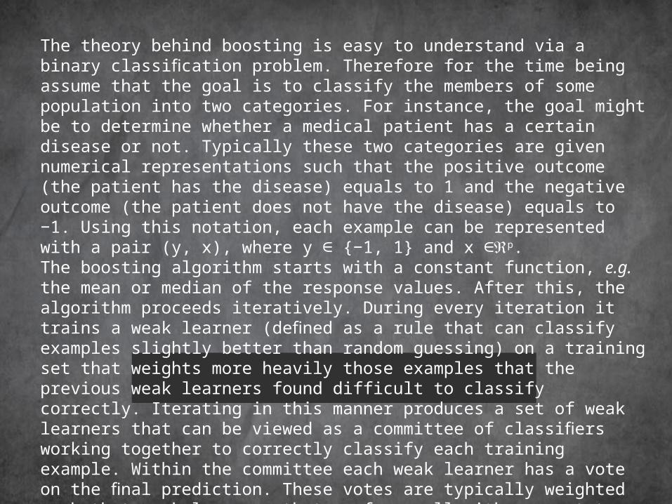
The theory behind boosting is easy to understand via a binary classification problem. Therefore for the time being assume that the goal is to clas sify the members of some population into two categories. For instance, the goal might be to determine whether a medical patient has a certain disease or not. Typi cally these two categories are given numerical representations such that the positive outcome (the patient has the disease) equals to 1 and the negative outcome (the pa tient does not have the disease) equals to −1. Using this notation, each example can be represented with a pair (y, x), where y ∈{−1, 1} and x ∈p. The boosting algorithm starts with a constant function, e.g. the mean or median of the response values. After this, the algorithm proceeds iteratively. During every it eration it trains a weak learner (defined as a rule that can classify examples slightly better than random guessing) on a training set that weights more heavily those ex amples that the previous weak learners found difficult to classify correctly. Iterating in this manner produces a set of weak learners that can be viewed as a committee of classifiers working together to correctly classify each training example. Within the committee each weak learner has a vote on the final prediction. These votes are typically weighted such that weak learners that perform well with respect to the training set have more relative influence on the final prediction. The weighted pre dictions are then added together. The sign of this sum forms the final prediction (resulting into a prediction of either +1 or -1) of the committee. And a GREAT space and time consumer is to put lots of unnecessary bibliographic material on your visuals, especially if they point to your own previous work and you can get them into a microscopically small font like this one that even you can’t read and have NO IDEA why you ever even put it in there in the first place!!

Averaging

Statisticians and Averages

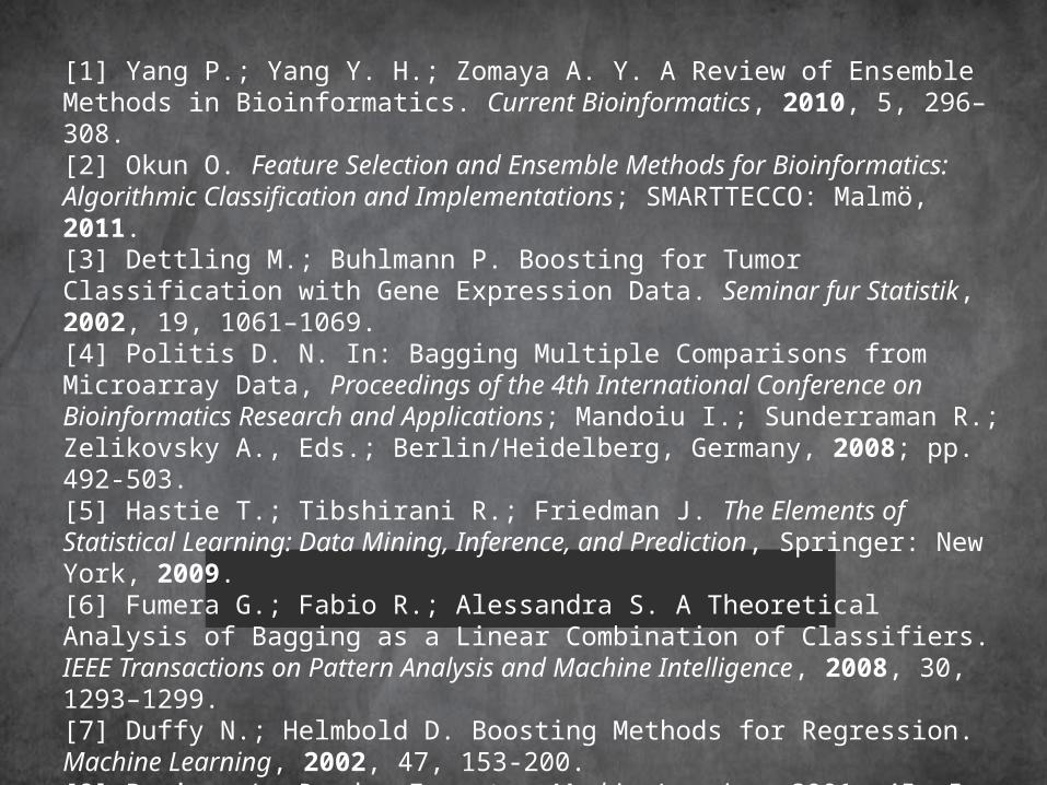
[1] Yang P.; Yang Y. H.; Zomaya A. Y. A Review of Ensemble Methods in Bioinformatics. Current Bioinformatics, 2010, 5, 296–308.[2] Okun O. Feature Selection and Ensemble Methods for Bioinformatics: Algorithmic Classification and Implementations; SMARTTECCO: Malmö, 2011.[3] Dettling M.; Buhlmann P. Boosting for Tumor Classification with Gene Expression Data. Seminar fur Statistik, 2002, 19, 1061–1069.[4] Politis D. N. In: Bagging Multiple Comparisons from Microarray Data, Proceedings of the 4th International Conference on Bioinformatics Research and Applications; Mandoiu I.; Sunderraman R.; Zelikovsky A., Eds.; Berlin/Heidelberg, Germany, 2008; pp. 492-503.[5] Hastie T.; Tibshirani R.; Friedman J. The Elements of Statistical Learning: Data Mining, Inference, and Prediction, Springer: New York, 2009.[6] Fumera G.; Fabio R.; Alessandra S. A Theoretical Analysis of Bagging as a Linear Combination of Classifiers. IEEE Transactions on Pattern Analysis and Machine Intelligence, 2008, 30, 1293–1299.[7] Duffy N.; Helmbold D. Boosting Methods for Regression. Machine Learning, 2002, 47, 153-200.[8] Breiman L. Random Forests. Machine Learning, 2001, 45, 5-32.[9] Freund Y.; Schapire R. E. A Decision-Theoretic Generalization of Online Learning and an Application to Boosting. Journal of Computer and System Sciences, 1997, 55, 119-139.

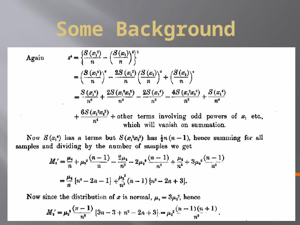
Some Background

Simulation

Results

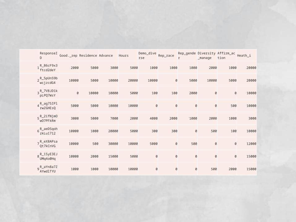
ResponseID Good._rep Residence Advance Hours Demo_diverse Rep_race Rep_gender Diversity_ma

nage Affirm_action Heath_i

1 R_86cF9x3ftcd2deY 2000 5000 3000 5000 1000 1000 1000 2000 1000 20000

2 R_5pUnS9bwcjzcdG4 10000 5000 10000 20000 10000 0 5000 10000 5000 20000

3 R_7V8JD1kpLPQ7WsY 0 10000 10000 5000 100 100 2000 0 0 10000

4 R_ag75IPlrwZGHEsQ 5000 5000 10000 10000 0 0 0 0 500 10000

5 R_2ifNjmOwO7PFkRm 3000 5000 7000 2000 4000 2000 1000 2000 1000 3000

6 R_aeDSqohzkLu1712 10000 1000 20000 5000 300 300 0 500 100 10000

7 R_eX8APsaQt7kCnVG 10000 500 30000 10000 5000 0 500 0 0 12000

8 R_1SyE3EJUMq4o0Hq 10000 2000 15000 5000 0 0 0 0 0 15000

9 R_aYn8a7ZAYwdlTYU 1000 1000 10000 10000 0 0 0 500 2000 15000

• Our method• Performed really well• In fact, in all the data sets we found

• Our method• Was the best• Was better than the other methods

• In all the data sets we simulated• Our method

• Was the best• Out performed the other methods

• Our method• Is faster and easier to compute and has the smallest

asymptotic variance compared to the other method that we found in the literature

• So, now I’d like to show some of the results from our simulation studies where we simulated data sets and tuned our method to optimize performance comparing it to the other method which we really didn’t know how to use

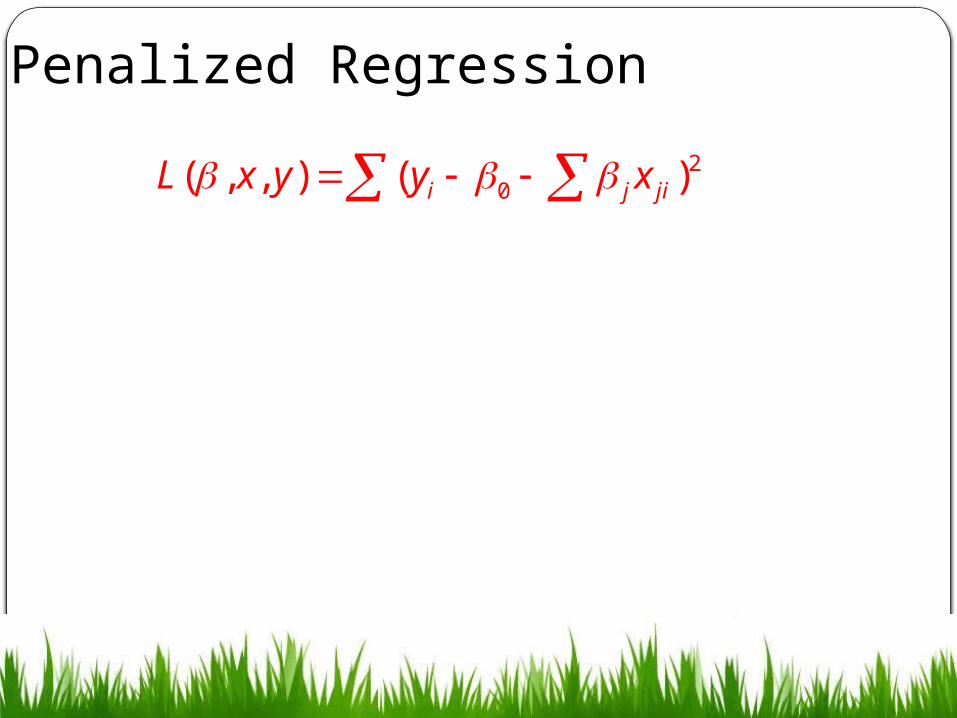
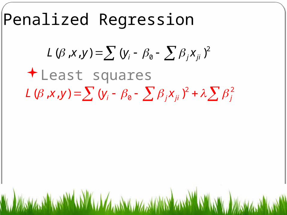
Penalized Regression

20( , , ) ( )i j jiL x y y x

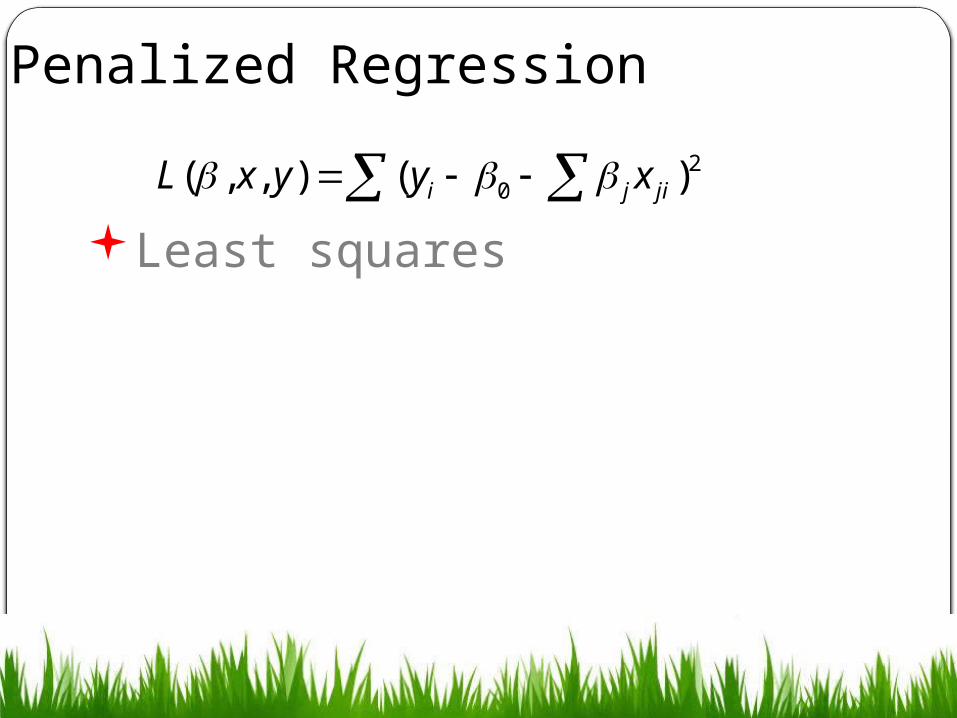
Penalized Regression

Least squares

20( , , ) ( )i j jiL x y y x

Penalized Regression

Least squares

20( , , ) ( )i j jiL x y y x

2 20( , , ) ( )i j ji jL x y y x

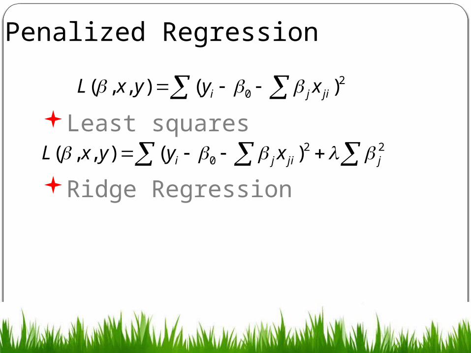
Penalized Regression

Least squares

Ridge Regression

20( , , ) ( )i j jiL x y y x

2 20( , , ) ( )i j ji jL x y y x

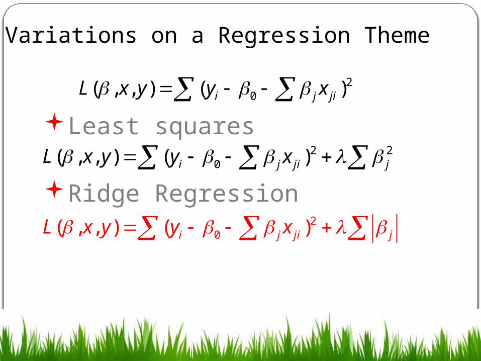
Variations on a Regression Theme

Least squares

Ridge Regression

20( , , ) ( )i j jiL x y y x

2 20( , , ) ( )i j ji jL x y y x

20( , , ) ( )i j ji jL x y y x

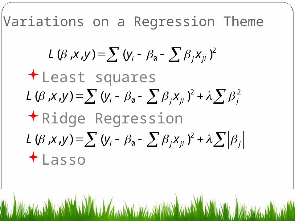
Variations on a Regression Theme

Least squares

Ridge Regression

Lasso

20( , , ) ( )i j jiL x y y x

2 20( , , ) ( )i j ji jL x y y x

20( , , ) ( )i j ji jL x y y x

Stepwise Regression ReviewForward Stepwise Regression – If we standardize x’s, start with r = y

Find x most correlated with rAdd x to fit, r=y-fitFind x most correlated with rContinue until no x is correlated enough

• LAR is similar (Forward Stagewise)– Only enter as much of x as it “deserves”• Find xj most correlated with r,• βj ← βj + δj , where δj = e sign <r, xj> until another

variable is equally correlated• Move βj and βk in the direction defined by their joint

least squares coefficient of the current residual on (xj ; xk), until some other competitor x has as much correlation with the current residual.• Set r ← r − new predictions and repeat steps many times

LAR and Lasso

• Boosting fits an Additive Model • Forward Stagewise Additive Modeling

1. f0(x) = 02. For m=1,…, M

a. Compute

b. Set , 1,

( , ) argmin ( ( ) ( ; ))m m i m i iL y f x b x

1( ) ( ) ( ; )m m m i mf x f x b x

Adaboost?Adaboost is a stagewise AM with

Basis functions are just the classifiers

( ( )),( ( )) yf xL y f x e

( ) { 1, 1}mF x

Solve the Exponential Loss Problem

1( ( ) ( ))

,

,

argmin i m i iy f x F x

F

Using exponential loss solve

e

How to Solve That?

1

( ( ))( )

,

( )( )

:

argmin i i

i m i

y F xmi

F

y f xmi

Find and F

w e

where

w e

Two Steps

( ( ))

( ) ( )

( )

,

argmi

arg i

n

m n

i iy F x

m mi i

F y

i

F

m

F

y F

For fixed find

w w

e

e

F

e

w

First Step

( ( ))( )

( ) ( )

( ) ( )argmin ( ) ( ( ))

,

argmin

argmin

i i

m mi i i i

F all y all y

y F xmi

F

m mi i

F y F y F

For fixed find F

w e

e w e

e e w I y

w

F x e w

End of First Step

( ( ))

( )

( )

( ) ( )

( ) ( )

,

argmin

argmin

argmin

argmin

( ) ( ( )

( (

)

))

i iy F xmi

F

m mi i

F y F y F

m mi i i i

F all y a

mm i i i

F al

l

l y

l y

For fixed find F

w e

e w e w

e e w I y F

F w I

x w

F

e

x

So

y

Almost There – what about ?b

( ) ( )

argmin ( )

argmin( ) ( ( ))m mi i i i

all y all y

Find

G

e e w I y F x e w

Take Derivative( ) (

)

)

( ( )

( )0

argmin ( )

( ) ( ( ))

( ) ( )

0

( )m m

m mi i i i

i i i iall y

all y all y

all y

G e e w I y F x e w

G

e e w I y F x e w

Almost There

2 ( ) 2 (

(

)

) ( )

(

( ) ( (

1 ) ( ( )) 0

)) 0m mi i i i

all y all y

m mi i i i

all y all y

e e w I y F

e w I y F x e w

x e w

Almost There

( ) ( )

( ) ( )

2 ( ) 2 (

2( )

)

( ( )

( ) ( ( )) 0

(1 ) ( ( ))

)

( ( )

0

)

m mi i i i

all y all y

m mi

m m

i i

i i i i

mi

iall y all

i i

y

e e w I y F x e w

e w I y F

w w I y F xe

w I y F x

x e w

And?

( ) ( )

2( )

( ( ))

( ( ))

11log2

m mi i i i

m

mm

m

i i i

w w I y F xe

w I y F x

Wait? What?So Adaboost

Finds the next “weak learner” that minimizes the sum of the weighted exponential missclassifications

With overall weights equal to Adds this to previous estimates11

log2

m

m

Where are we?Adaboost is:

Forward stagewise additive modelWith exponential loss function

Sensitive to misclassification since we use exponential (not missclassification) loss

Now what – extend to regression?Why exponential loss?

Squared error loss is least squaresWhat’s more robust?

Absolute Error lossHuber lossTruncated loss

Next IdeaGradient Boosting MachineTake these ideas:

Loss function Find Just solve this by steepest descent

( ) ( , ( ))i iL f L y f x

ˆ argmin ( )f

f L f

Oops --- one small problem

The derviatives are based only on the training data They won’t generalize

So calculate them and “fit” them using trees

Boosted Trees

Making it more Robust

Can handle 25% contamination to original data set

Some

Applicatio

ns

Wine Data Set

11 predictors and a ratingInput variables (based on physicochemical tests): 

1 - fixed acidity 2 - volatile acidity 3 - citric acid 4 - residual sugar 5 - chlorides 6 - free sulfur dioxide 7 - total sulfur dioxide 8 - density 9 - pH 10 - sulphates 11 - alcohol 

Output variable (based on sensory data): 12 - quality (score between 0 and 10)

Performance Under Contamination- Red Wine

Performance Under Contamination- White Wine

• Our method• Performed really well• In fact, in all the data sets we found

• Our method• Was the best• Was better than the other methods

• In all the data sets we simulated• Our method

• Was the best• Out performed the other methods

• Our method• Is faster and easier to compute and has the smallest asymptotic variance

compared to the other method that we found in the literature