Dicing - pku.edu.cn

DicingChen Yunchuan

2015.4.29

Outline• Sampling

• Random Variable Generation

• Rejection Sampling

• Importance Sampling

• Markov Chain Monto Carlo (MCMC)

• Restricted Boltzmann Machine Revisit

• Learning algorithms

• Imagination: Represent Word with Random Vectors

Example of Monte Carlo: Estimate 𝜋

• Estimate 𝜋

⇡ ⇡ 4Nhits

N

Estimating 𝜋

Draw i.i.d. set of samples {x(i)}Ni=1

from a target density p(x| · )Z

Xf(x)p(x| · )dx ⇡ 1

N

NX

i=1

f(x(i))

⇡

4=

SCSD

=

RRC dxdyRRD dxdy

=

RRC p(x, y)dxdyRRD p(x, y)dxdy

=

ZZ

D{(x, y) 2 C}p(x, y)dxdy

⇡ 1

N

NX

i=1

{(x(i), y

(i)) 2 C} =Nhit

N

𝒟𝒞

Another Way to Estimate 𝜋

⇡ ⇡ 2lN

aNhits

Estimating 𝜋

phit =Sg

SG=

R ⇡0

l

2sin' d'

1

2a⇡

=2l

⇡a

phit ⇡Nhits

N⇡ ⇡ 2lN

aNhits

g

G

Estimating 𝜋

2l

⇡a

=Sg

SG=

RRg dxdyRRG dxdy

=

RRg p(x, y) dxdyRRG p(x, y) dxdy

=

ZZ

G{(x, y) 2 g}p(x, y) dxdy

= E[ {(x, y) 2 g}]

⇡ 1

N

NX

i=1

{(x, y) 2 g} =Nhits

N

g

G

Monte Carlo: Motivation

• Estimation

• Optimization

• Model Selection

Random Variable Generation

• where F

�(u) = inf{x : F (x) � u}

if U ⇠ U[0,1], then the random variable F�(U) has the distribution F

• The theorem above is theoretical beautiful, but unpractical in real application

• It is hard to compute the generalized inverse function

• High dimensional cases?

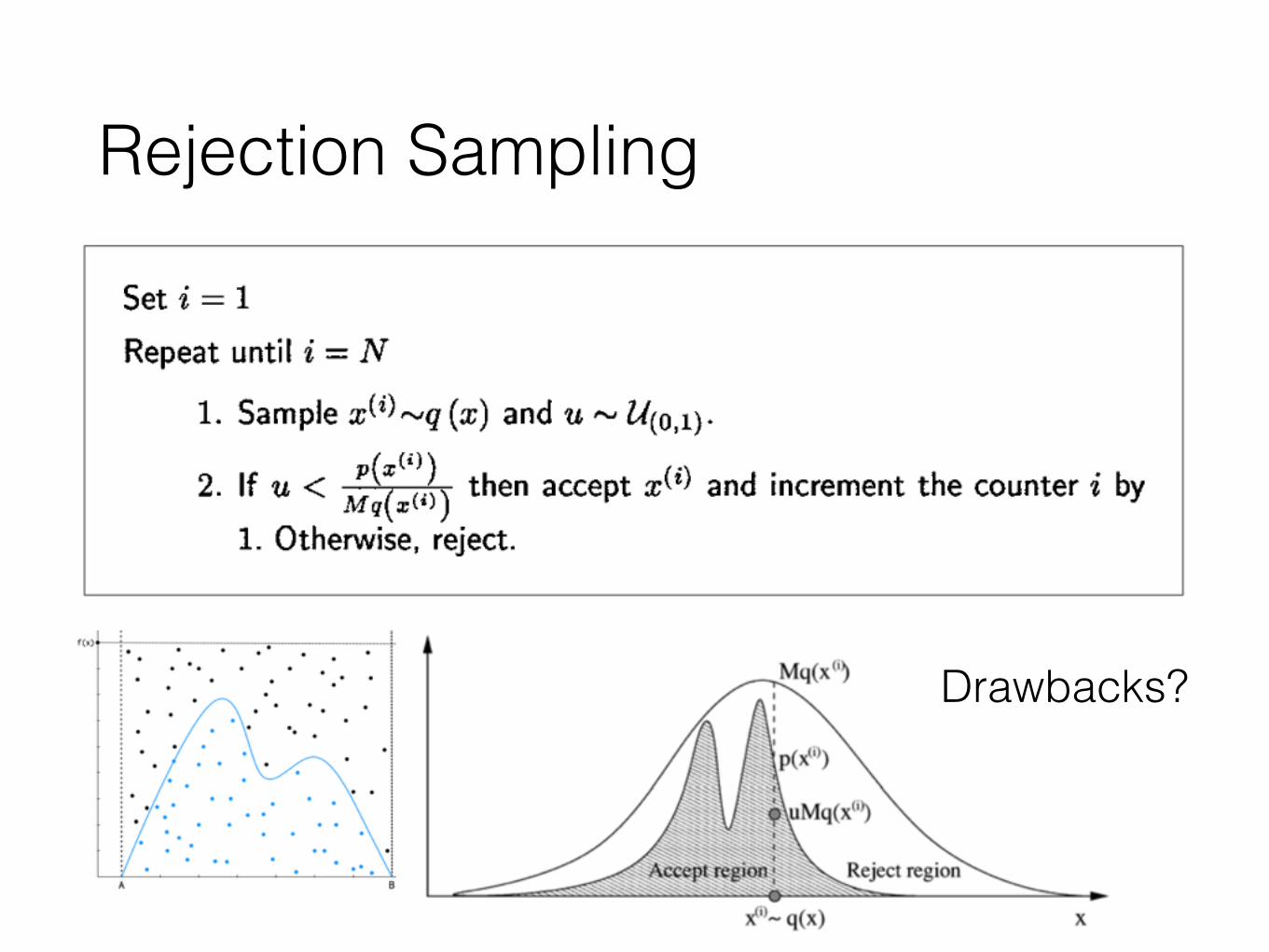
Rejection Sampling

Drawbacks?

Importance SamplingZ

f(x)p(x) dx =

Zf(x)

p(x)

q(x)q(x) dx

⇡ 1

N

NX

i=1

f(x(i))p(x(i))

q(x(i))

• Does the i.i.d. property necessary for estimating an integral?

Another 𝜋 Estimation Story

Stationary Stochastic Process

E[Xt] = constant = lim

T!+1

1

T

Z T

0X(t) dt

E[f(Xt)] = limT!+1

1

T

Z T

0f(X(t)) dt

Why ?E[f(Xt)] = limT!+1

1

T

Z T

0f(X(t)) dt

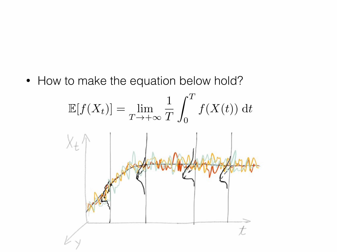
• How to make the equation below hold?

E[f(Xt)] = limT!+1

1

T

Z T

0f(X(t)) dt

Markov Chain Monte Carlo (MCMC): Intuitions

MCMC: Important Theoretical Results

• Irreducibility

• Aperiodicity

• Detailed Balance Condition⇡iPij = ⇡jPji

410 2 31

10.5 0.5 0.5

0.5 0.5 0.5

MCMC: Applications to Sampling Algorithms: Metropolis-Hastings Alg. (MHA)

• Proposal Distribution

↵(i, j) = A(x(i), x

(j))

q(i, j) = q(x(j)|x(i))

• Acceptance Prob.

• Detailed Balance

• Target Distribution⇡(i) = p(x(i))

⇡(i)q(i, j)↵(i, j) = ⇡(j)q(j, i)↵(j, i) ↵(i, j) = min{1, ⇡(j)q(j, i)⇡(i)q(i, j)

}

Special Cases of MHA• Independent Sampler: Assuming that the proposal

is independent of the current state

↵(i, j) = min

⇢1,

p(x(j))q(x(i))

p(x(i))q(x(j))

�= min

⇢1,

w(x(j))

w(x(i))

�q(x(j)|x(i)) = q(x(j))

• Metropolis Sampler: Assuming that the proposal is symmetric

q(x(j)|x(i)) = q(x(i)|x(j))

↵(i, j) = min

⇢1,

p(x(j))

p(x(i))

�

• Gibbs Sampler: Good property: no rejections

MHA Running Examples

Simulated Annealing (SA)• Annealing is the process of heating a solid until thermal

stresses are released. Then, in cooling it very slowly to the ambient temperature until perfect crystals emerge. The quality of the results strongly depends on the cooling temperature. The final state can be interpreted as an energy state (crystaline potential energy) which is lowest if a perfectly crystal emerged

Pr(x) =

1

Zexp(�E(x)/kBT )

Pr(x ! xp) =

(1, �E < 0;

exp(��E/kBT ), �E � 0.

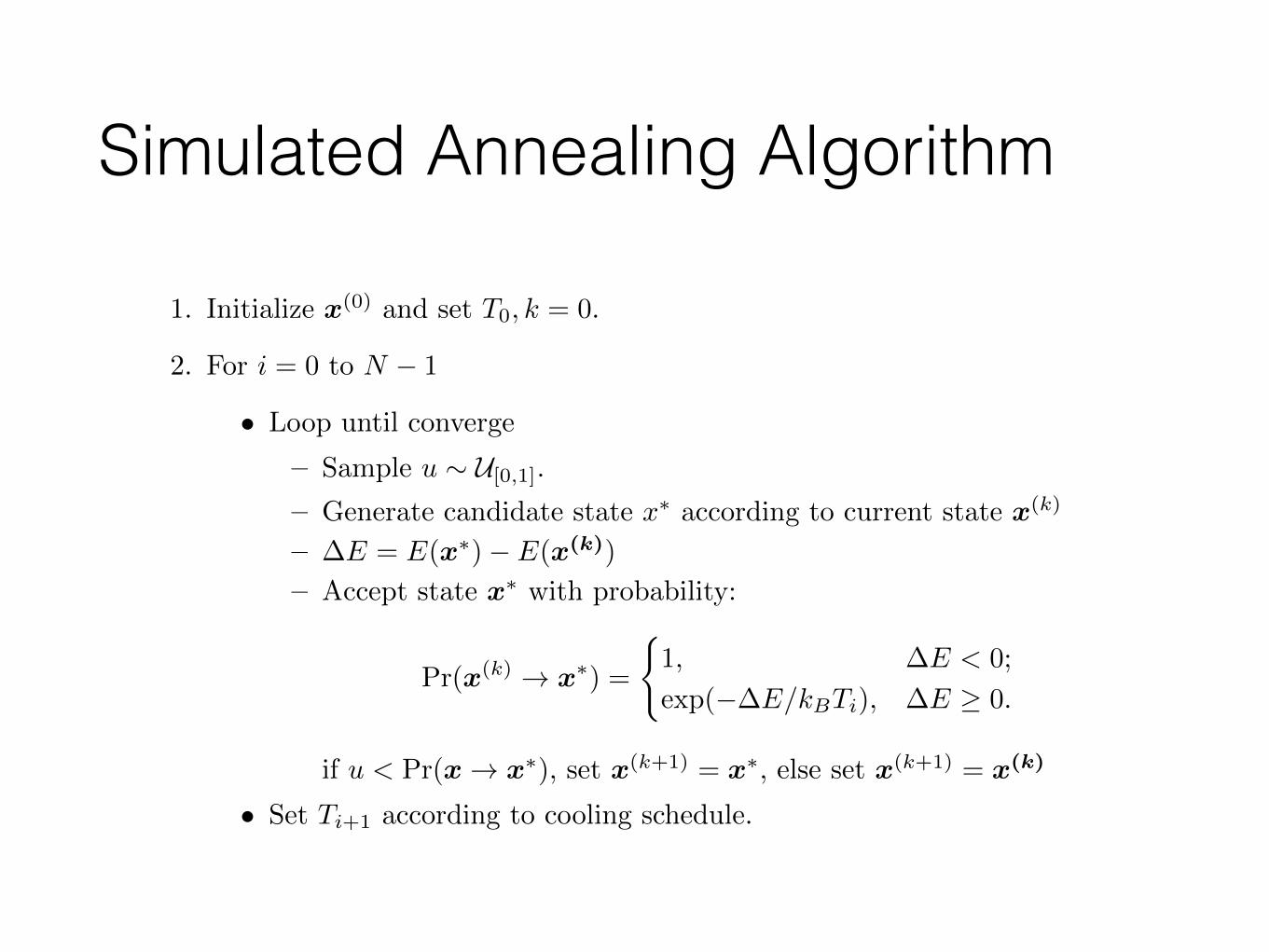
Simulated Annealing Algorithm

1. Initialize x

(0)and set T0, k = 0.

2. For i = 0 to N � 1

• Loop until converge

– Sample u ⇠ U[0,1].

– Generate candidate state x

⇤according to current state x

(k)

– �E = E(x

⇤)� E(x

(k))

– Accept state x

⇤with probability:

Pr(x

(k) ! x

⇤) =

(1, �E < 0;

exp(��E/kBTi), �E � 0.

if u < Pr(x ! x

⇤), set x

(k+1)= x

⇤, else set x

(k+1)= x

(k)

• Set Ti+1 according to cooling schedule.

Simulated Annealing Algorithm

Toy Example: Maximization

Solve Traveling Salesman Problem with SA

0 200 400 600 800 1000 120020

40

60

80

100

120

140

160

20 cities Initial configuration

Restricted Boltzmann Machine (RBM)

A =

0

BBB@

h1v1 h1v2 . . . h1vnh2v1 h2v2 . . . h2vn...

.... . .

...hmv1 hmv2 . . . hmvn

1

CCCAW =

0

BBB@

w11 w12 . . . w1n

w21 w22 . . . w2n...

.... . .

...wm1 wm2 . . . wmn

1

CCCA

E(v,h) = �v

TWh� b

Tv � c

Th

= �mX

i=1

nX

j=1

wijhivj �nX

j=1

bjvj �mX

i=1

cihi

= �W �A� b

Tv � c

Th

= �✓

T�(x)

Basics to Learn RBM

✓ = [W (:); b; c]

�(x) = [A(:);v;h]

• Fitting p(v) to data

p(v) =1

Z

X

h

exp(�E(v,h))

• Notations

Learning RBM: Maximum Likelihood Estimation

@ log p(v0;✓)

@wij= Ep(h|v0;✓)[hivj ]� Ep(x;✓)[hivj ]

@ log p(v0;✓)

@✓= Ep(h|v0;✓)�(v0,h)� Ep(x;✓)[�(x)]

1

`

X

v2S

@ log p(v;✓)

@wij= Ep(h|v;✓)q(v)[hivj ]� Ep(x;✓)[hivj ]

S = {v1,v2, . . . ,v`}

• Given Observed Samples

• We can get

for

Intractable

k-Step Contrastive Divergence Alg.

CD-k Running Examples

Note: from bottom to top k = 1, 2, 5, 10, 20, 100

• Persistent Contrastive Divergence (PCD)

• Fast Persistent Contrastive Divergence (FPCD)

• Stochastic Approximation Procedure (SAP)

• Stochastic Approximation Procedure with Tempered Transitions (Trans-SAP)

• Parallel Tempering (PT)

Other Algorithms for Training RBM

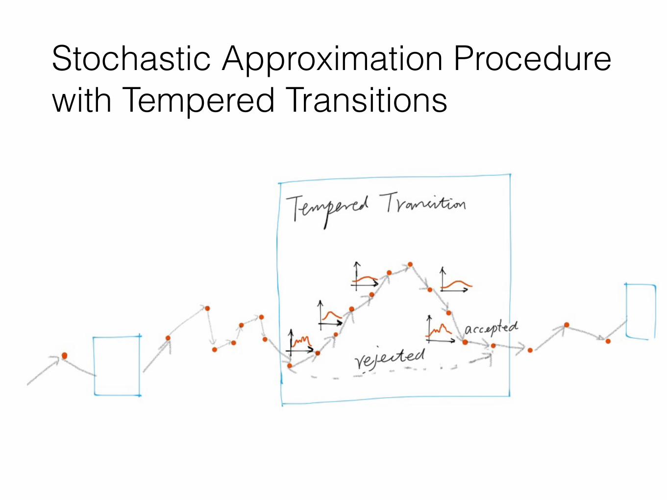
Stochastic Approximation Procedure with Tempered Transitions

Parallel Tempering

Parallel Tempering v.s. CD-k: Running Examples (1/2)

PT CD-k

Note: from bottom to top k = 1, 2, 5, 10, 20, 100 Note: bottom to top M = 4,5,10,50

Parallel Tempering v.s. CD-k: Running Examples (2/2)

Positive Samples Negative Samples

References• Andrieu, Christophe, Nando de Freitas, Arnaud Doucet, and Michael I Jordan. ‘An Introduction to

MCMC for Machine Learning.’, Machine learning, 2003

• Fischer, Asja, and Christian Igel. ‘Training restricted Boltzmann machines: An introduction.’, Pattern Recognition, 2014

• Salakhutdinov, Ruslan. ‘Learning in Markov Random Fields using Tempered Transitions.’, NIPS, 2009

• Geoffrey E. Hinton, Simon Osindero, Simon Osindero, and Yee-Whye Teh. ‘A Fast Learning Algorithm for Deep Belief Nets’, Neural computation, 2006

• Desjardins, Guillaume, Aaron C Courville, Yoshua Bengio, Pascal Vincent, and Olivier Delalleau. ‘Parallel Tempering for Training of Restricted Boltzmann Machines ’, AISTATS, 2010

• Neal, Radford M. ‘Sampling from multimodal distributions using tempered transitions’, Statistics and computing, 1996

• Geoffrey E. Hinton. ‘Reducing the Dimensionality of Data with Neural Networks’, Science, 2006

• Cho, Kyunghyun, Tapani Raiko, and Alexander Ilin. ‘Parallel tempering is efficient for learning restricted Boltzmann machines’, International Joint Conference on Neural Networks (IJCNN), 2010

Thanks

Dicing - pku.edu.cn

Documents

Transcript of Dicing - pku.edu.cn