remote sensing

Article

Diagnostics of Es Layer Scintillation Observations UsingFS3/COSMIC Data: Dependence on Sampling Spatial Scale

Lung-Chih Tsai 1,2,*, Shin-Yi Su 2, Chao-Han Liu 3, Harald Schuh 4,5 , Jens Wickert 4,5

and Mohamad Mahdi Alizadeh 4,6

�����������������

Citation: Tsai, L.-C.; Su, S.-Y.;

Liu, C.-H.; Schuh, H.; Wickert, J.;

Alizadeh, M.M. Diagnostics of Es

Layer Scintillation Observations

Using FS3/COSMIC Data:

Dependence on Sampling Spatial

Scale. Remote Sens. 2021, 13, 3732.

https://doi.org/10.3390/rs13183732

Academic Editor: Guillermo

Gonzalez-Casado

Received: 24 August 2021

Accepted: 14 September 2021

Published: 17 September 2021

Publisher’s Note: MDPI stays neutral

with regard to jurisdictional claims in

published maps and institutional affil-

iations.

Copyright: © 2021 by the authors.

Licensee MDPI, Basel, Switzerland.

This article is an open access article

distributed under the terms and

conditions of the Creative Commons

Attribution (CC BY) license (https://

creativecommons.org/licenses/by/

4.0/).

1 GPS Science and Application Research Center, National Central University (NCU), Taoyuan 320317, Taiwan2 Center for Space and Remote Sensing Research, National Central University (NCU), Taoyuan 320317, Taiwan;

sysu@csrsr.ncu.edu.tw3 Academia Sinica, Taipei 115024, Taiwan; chliu2@gate.sinica.edu.tw4 Institute of Geodesy and Geoinformation Science, Technische Universität Berlin, 10623 Berlin, Germany;

schuh@gfz-potsdam.de (H.S.); wickert@gfz-potsdam.de (J.W.); alizadeh@tu-berlin.de (M.M.A.)5 German Research Centre for Geosciences GFZ, 14473 Potsdam, Germany6 Department of Geodesy and Geomatics Engineering, K. N. Toosi University of Technology, Tehran 19697, Iran* Correspondence: lctsai@csrsr.ncu.edu.tw

Abstract: The basic theory and experimental results of amplitude scintillation from GPS/GNSS radiooccultation (RO) observations on sporadic E (Es) layers are reported in this study. Considering an Eslayer to be not a “thin” irregularity slab on limb viewing, we characterized the corresponding electrondensity fluctuations as a power-law function and applied the Ryton approximation to simulate spatialspectrum of amplitude fluctuations. The scintillation index S4 and normalized signal amplitudestandard deviation S2 are calculated depending on the sampling spatial scale. The theoretical resultsshow that both S4 and S2 values become saturated when the sampling spatial scale is less than the firstFresnel zone (FFZ), and S4 and S2 values could be underestimated and approximately proportionalto the logarithm of sampled spatial wave numbers up to the FFZ wave number. This was verifiedby experimental analyses using the 50 Hz and de-sampled FormoSat-3/Constellation ObservingSystem for Meteorology, Ionosphere and Climate (FS3/COSMIC) GPS RO data in the cases of weak,moderate, and strong scintillations. The results show that the measured S2 and S4 values have avery high correlation coefficient of >0.97 and a ratio of ~0.5 under both complete and undersamplingconditions, and complete S4 and S2 values can be derived by dividing the measured undersamplingS4 and S2 values by a factor of 0.8 when using 1-Hz RO data.

Keywords: ionospheric scintillation; ionospheric Es layer; GPS/GNSS radio occultationobservation; COSMIC

1. Introduction

Sporadic E (Es) layers exhibit ionization enhancements in the E region at altitudesusually between 90 and 120 km [1]. A characteristic feature of Es layers is that they are thinlayers of a few kilometers’ thicknesses and a 10~1000 km horizontal extension. Over thepast few decades, since the 1950s, Es layers have been extensively studied using a varietyof instruments, including ionosondes, incoherent scatter radars and coherent scatter veryhigh-frequency (VHF) radars operating from the ground and in rocket payloads with in-situmeasurements. Several excellent reviews of the theories and observations of ionosphericEs layers have also been published [1–4]. It is generally believed that Es layer structureis affected by the plasma convergence effect of neutral wind shear through ion-neutralcollision processes at mid and low latitudes [1]. Es layers could appear as non-uniformwave layers, a composition of irregular elongated clouds of intense ionization, or multiplelayers, occurring simultaneously and separated by several kilometers within the lower Eregion [5]. Therefore, this gradient plasma instability can give rise to irregularities, with

Remote Sens. 2021, 13, 3732. https://doi.org/10.3390/rs13183732 https://www.mdpi.com/journal/remotesensing

Remote Sens. 2021, 13, 3732 2 of 14

scale-sizes from a few tens of meters to a few kilometers, which can produce VHF/UHFradio wave scattering, and cause signal scintillations in satellite radio communication andnavigation system performance [6].

The Global Positioning System (GPS) or Global Navigation Satellite System (GNSS)RO techniques provide an innovative view of the ionosphere via horizontal limb soundingfrom GPS/GNSS satellites to low-Earth-orbiting (LEO) satellites. There have been manysuccessful GNSS-LEO RO missions, such as GPS/Meteorology, the Danish Ørsted, theGerman CHAMP (Challenging Mini-satellite Payload), the U.S.–German GRACE (GravityRecovery and Climate Experiment), the GPS-IOX (Ionospheric Occultation Experiment),the Argentinean SAC-C (Satellite de Aplicaciones Cientificas-C), the Taiwan–U.S. COSMIC,and the Taiwan–U.S. COSMIC2. Based on these GPS/GNSS RO missions’ data, more Eslayer studies have been presented [5,7–11]. Notably, in most of the above investigations,the criteria to identify Es events include that the peak normalized amplitude standarddeviation of GPS/GNSS RO observations at E-region altitudes is higher than 0.2. However,this presents a problem for scintillation data for which the limb-viewing amplitudes ofsome of the GNSS-LEO RO missions were obtained at a sampling frequency less than theFresnel frequency fF, i.e., a sampling spatial scale larger than the first Fresnel zone (FFZ).Such undersampling had not happened in earlier Es layer investigations using incoherentscatter radars and coherent scatter VHF radars operating from the ground and in rocketpayloads with in situ measurements. Thus, it is desirable to clarify the dependence onsampling spatial scale of scintillation index determination, and find a method of solvingreliable scintillation indexes (S4 and S2) under undersampling conditions on GPS/GNSSRO observations.

In the following section, we introduce the Ryton approximation for radio wave propa-gations through an Es layer irregularity slab, and simulate the scintillation index S4 andnormalized signal amplitude standard deviation S2 values, depending on the samplingspatial scale. In Section 3, we analyze the 50 Hz FS3/COSMIC RO amplitude data and thecorresponding de-sampled data to prove the dependence of S4 and S2 determinations onsampling spatial scale. In Section 4, we present the reliability of complete S4 and S2 deter-minations using undersampling S4 and S2 measurements. In conclusion, we summarizethe usefulness of the results.

2. Methods and Materials

When a radio wave transmitted by a satellite passes through the ionosphere, itswavefront will be distorted by irregular electron densities, i.e., plasma densities. After theradio wave has emerged from an irregularity slab, its phase front is randomly modulated.It is assumed that the deviation and the change in the refractive index over a spatialrange of one wavelength and a temporal range of one wave period are slight. Undersuch a condition, the small-angle scattering of a layer of plasma density turbulence causesspatial and temporal fluctuations of radio wave intensity and phase, which is known asscintillation. In this study, we focus on the diagnostics of amplitude scintillation duringGPS/GNSS RO observations carried out on Es layers.

Let us assume the geometry of an Es layer scintillation problem in GPS/GNSS RO ob-servations, as shown in Figure 1. A region of irregular electron density structures is locatedfrom x = −L/2 to x = L/2, where L could be the cutoff length of a GPS-LEO limb viewinglink through an Es layer. A time-harmonic electromagnetic wave is transmitted by a GNSSsatellite located at x =−∞, and it is incident on an Es layer slab at x =−L/2 and received byan LEO satellite receiver at a specific coordinate (x, ρt), where ρt = (y, z) is the transverse co-ordinate of wave propagation. The small-angle scattering of the scintillation phenomenonreduces the propagation equation of a wave field, where E = u(x, ρt) exp(−i k x), to theparabolic wave equation in u(x, ρt), as follows [12].

− 2jk∂u∂x

+ ∇2t u = −k2ε1(x, ρt) u , (1)

Remote Sens. 2021, 13, 3732 3 of 14

where –L/2 < x < L/2, and ∇2t = ∂2/∂2

y + ∂2/∂2z .

− 2jk∂u∂x

+ ∇2t u = 0 , (2)

where x > L/2. Here, ε1(x, ρt) is the fluctuating part of dielectric permittivity ε(x, ρt).Equations (1) and (2) are of the parabolic type, whose solutions are determined uniquelyby the boundary conditions at x = −L/2 and x = L/2, respectively. Notably, the irregularityslab can be characterized by its dielectric permittivity, as follows.

ε(x, ρt) = 〈ε〉 [1 + ε1(x, ρt)] = [1 −(

fp0/ f) 2] ε0 [1 + ε1(x, ρt)] , (3)

and

ε1(x, ρt) = −(

fp0/ f)2

[∆N(x, ρt)/N0]

1−(

fp0/ f) 2 ≈ − e2

4π2 ε0 m f 2 ∆N(x, ρt) , (4)

where ∆N(x, ρt) is the fluctuating part of electron density, and fp0 is the plasma frequencycorresponding to the background electron density N0. f is the radio wave frequency, i.e.,GPS L1- or L2-band frequency, and is much larger than fp0. The other constants includethe electronic charge e, the electronic mass m, and the free space permittivity ε0. Notably,ε1(x, ρt) is proportional to the fluctuating part of electron density ∆N(x, ρt) but is in inverseproportion to the square of radio wave frequency f. In this study, we do not consider theeffects of wave propagation through an elongated Es layer cloud and/or multiple Es layers.It will be interesting to work on this in future investigations.

Remote Sens. 2021, 13, x FOR PEER REVIEW 3 of 15

,),(2 122 uxku

xujk tt ρε−=∇+

∂∂− (1)

where –L/2 < x < L/2, and 22222zyt ∂∂+∂∂=∇ .

,02 2 =∇+∂∂− uxujk t (2)

where x > L/2. Here, ε1(x, ρt) is the fluctuating part of dielectric permittivity ε(x, ρt). Equa-tions (1) and (2) are of the parabolic type, whose solutions are determined uniquely by the boundary conditions at x = −L/2 and x = L/2, respectively. Notably, the irregularity slab can be characterized by its dielectric permittivity, as follows.

( ) ,)],(1[]/1[)],(1[),( 102

01 tptt xffxx ρεερεερε +−=+= (3)

and

( ) [ ]( ) ,),(

4/1/),(/

),( 20

2

2

20

02

01 t

p

tpt xN

fme

ffNxNff

x ρεπ

ρρε Δ−≈

−Δ

−= (4)

where ΔN(x, ρt) is the fluctuating part of electron density, and fp0 is the plasma frequency corresponding to the background electron density N0. f is the radio wave frequency, i.e., GPS L1- or L2-band frequency, and is much larger than fp0. The other constants include the electronic charge e, the electronic mass m, and the free space permittivity ε0. Notably, ε1(x, ρt) is proportional to the fluctuating part of electron density ΔN(x, ρt) but is in inverse proportion to the square of radio wave frequency f. In this study, we do not consider the effects of wave propagation through an elongated Es layer cloud and/or multiple Es lay-ers. It will be interesting to work on this in future investigations.

Figure 1. Geometry of an Es layer scintillation problem on GPS/GNSS RO observations. The origin is allocated as the point at which the Es layer’s center is projected onto the Earth’s surface. The x and z axes point in the GPS-LEO limb’s viewing direction and the azimuth direction, respectively.

It is now generally accepted that ionospheric electron density irregularities can be characterized by a power-law function [3,13–16]. To characterize the general power-law irregularity spectrum with spatial index p, [17] introduced a fairly general correlation spectrum, as follows.

Figure 1. Geometry of an Es layer scintillation problem on GPS/GNSS RO observations. The originis allocated as the point at which the Es layer’s center is projected onto the Earth’s surface. The x andz axes point in the GPS-LEO limb’s viewing direction and the azimuth direction, respectively.

It is now generally accepted that ionospheric electron density irregularities can becharacterized by a power-law function [3,13–16]. To characterize the general power-lawirregularity spectrum with spatial index p, [17] introduced a fairly general correlationspectrum, as follows.

Φ∆N(κ) =σ2

N Γ( p

2)

κp−30

π3/2 Γ(

p−32

) (κ2 + κ20

)−p/2∝ κ−p , (5)

where κ0 is the wave number of the outer scale l0 (=2π/κ0) in an irregularity slab, andΓ( ) is the Gamma function. The outer scale is defined as an intrinsic property of theinstability that causes electron density and plasma irregularities. The power-law continuumencompasses at least three orders of magnitude in the spatial scale size [13]. Notably, thepower-law spectrum is expected to be valid when its spatial scale is much less than the outerscale. In practice, it conforms to a GPS-LEO limb viewing an Es layer with a 10~1000 kmhorizontal extension.

Remote Sens. 2021, 13, 3732 4 of 14

Historically, the first ionospheric scintillation theory was based on the idea of wavediffraction from a phase-changing screen, and named phase screen theory [14,15,18]. Thisassumes that, as the radio waves propagate through an irregularity slab, to the first order,only the phase is affected by the random fluctuations in refractive index. The phase screentheory can be applied for the weak scintillations usually induced by a “thin” irregularityslab. Ref. [11] derived an Es layer thickness of 1.2 km at a peak distribution based onthe 50 Hz “atmPhs” FS3/COSMIC data. Considering such an Es layer distributed at analtitude of 100 km and along the Earth’s curvature, the cutoff length of a GPS-LEO limb’sviewing link through the Es layer is approximately 160 km, taken as the value of L inFigure 1. Therefore, we consider here that the Es layer in limb viewing is not a thinirregularity slab. The effects of scattering on the field amplitude inside a limb viewingirregularity slab must be included in the treatment of the Es layer scintillation phenomenon.Earlier investigations [13,19,20] derived the Ryton approximation for the parabolic waveEquations (1) and (2), and concluded that the Ryton approximation can be applied to weakand even strong ionospheric scintillations. Using the Ryton approximation, a wave fieldcan be presented in terms of the fluctuation of a complex phase ψ(x, ρt), shown as follows:

u (x, ρt) = u0 exp [ψ(x, ρt)] = u0 exp [χ(x, ρt) − jS1(x, ρt)] , (6)

where u0 is the average field of u(x, ρt) and is a reference field with definite amplitudeand phase. χ(x, ρt) and S1(x, ρt) are referred to as the log-amplitude and the phasedeparture of a wave field, respectively. The general Ryton solution of the parabolic waveEquations (1) and (2) was obtained as follows.

ψ(x, ρt) = j k2π( x+L/2)

sψ0(−L/2, ρ′t) exp

[−j k |ρt − ρ′t |

2

2 (x+L/2)

]d2ρ′t +

k2

4π

∫ x− L

2

dζx−ζ

sε1(ζ, ρ′t) exp

[−j k |ρt − ρ′t |

2

2 (x−ζ)

]d2ρ′t ,

(7)

where –L/2 < x < L/2.

ψ(x, ρt) =j k

2π (x− L/2)

xψ(L/2, ρ′t) exp

[−j k |ρt − ρ′t |

2

2 (x− L/2)

]d2ρ′t, (8)

where x > L/2. Notably, ψ0(−L/2, ρt) = ln u(−L/2, ρt) corresponds to the incident wave ofthe irregular slab, and ψ(L/2, ρt) = ln u(L/2, ρt) is its boundary condition at x = L/2.

In this study, we develop a plane incident wave with unity amplitude to be incidenton an Es layer slab in a limb-viewing direction. The small scattering angle assumptionmeans that the mean values of the log-amplitude and phase departures of the wave fieldthrough an Es layer slab are approximately zero, i.e., <χ> ~ <S1> ~ 0. The power spectrafor χ and S1 are given, respectively, by [21], as follows.

Φχ(0, κt) =π k2L

4

[1− 2k

κ2t L

sin(

κ2t L2k

)cos(

κ2t (x− L/2)

k

)]Φε1(0, κt) . (9)

ΦS1(0, κt) =π k2L

4

[1 +

2kκ2

t Lsin(

κ2t L2k

)cos(

κ2t (x− L/2)

k

)]Φε1(0, κt) . (10)

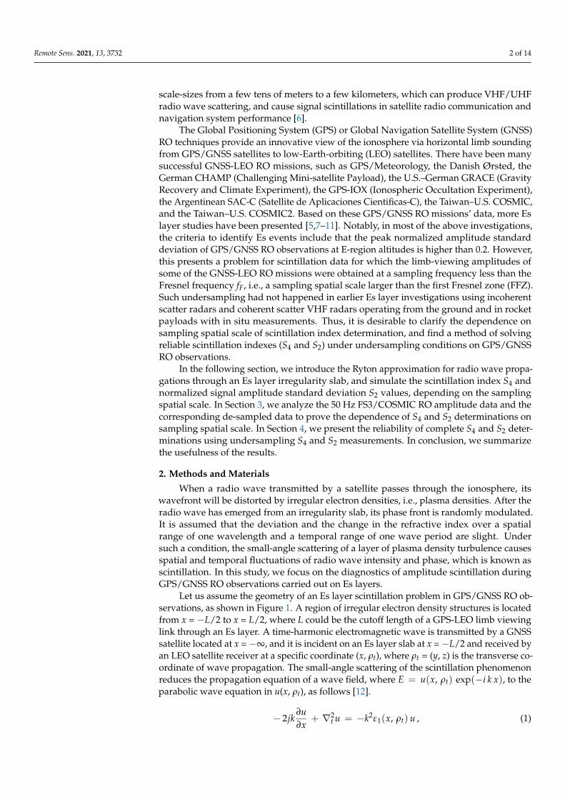
As shown in Figure 1, x is the distance from the center of an irregularity slab tothe receiver on an LEO satellite, and is equal to D (~3500 km) for a GPS/GNSS ROobservation on Es layers. κt is the wave number of a transverse spatial scale ρt. Notably, thespatial power spectrum of the log amplitude departure of wave field is controlled by twocompeting factors: a Fresnel filter function, shown as the expression in the square bracketsin Equation (9), and the power-law function of dielectric permittivity or electron densityfluctuation. Figure 2 shows the Fresnel filter as a function of normalized wave number κt/κF,where κF (=2π/DF) is the wave number in the first Fresnel zone (FFZ) DF (=

√λ D=~0.8 km)

Remote Sens. 2021, 13, 3732 5 of 14

corresponding to the GPS L1-band signal and a distance D of approximately 3500 kmfrom the Es layer slab to the LEO satellite during a GPS/GNSS RO observation. Theoscillatory character of the filter function is known as the Fresnel oscillation [3]. In Figure 2,the spatial power spectrum of the simulated log amplitude departure of wave field fromEquation (9) is also shown at a spatial index p of 4. The spatial spectrum is generallyof a power-law type with an order of p that decays as κt increases. It has a maximumaround κt = κF, corresponding to the first maximum of the Fresnel filter function. This isconsistent with an irregularity size in the order of FFZ, which is most effective in causingamplitude scintillation.

Remote Sens. 2021, 13, x FOR PEER REVIEW 5 of 15

through an Es layer slab are approximately zero, i.e., <χ> ~ <S1> ~ 0. The power spectra for χ and S1 are given, respectively, by [21], as follows.

( ) ( ),0)2/(cos2

sin214

,01

22

2

2

ttt

tt k

LxkL

LkLk κκκ

κπκ εχ Φ

−

−=Φ (9)

( ) ( ),0)2/(cos2

sin214

,01

22

2

2

1 ttt

ttS k

LxkL

LkLk κκκ

κπκ εΦ

−

+=Φ (10)

As shown in Figure 1, x is the distance from the center of an irregularity slab to the receiver on an LEO satellite, and is equal to D (~3500 km) for a GPS/GNSS RO observation on Es layers. κt is the wave number of a transverse spatial scale ρt. Notably, the spatial power spectrum of the log amplitude departure of wave field is controlled by two com-peting factors: a Fresnel filter function, shown as the expression in the square brackets in Equation (9), and the power-law function of dielectric permittivity or electron density fluctuation. Figure 2 shows the Fresnel filter as a function of normalized wave number κt/κF, where κF (=2π/DF) is the wave number in the first Fresnel zone (FFZ) DF (= Dλ=~0.8 km) corresponding to the GPS L1-band signal and a distance D of approximately 3500 km from the Es layer slab to the LEO satellite during a GPS/GNSS RO observation. The oscillatory character of the filter function is known as the Fresnel oscillation [3]. In Figure 2, the spatial power spectrum of the simulated log amplitude departure of wave field from Equation (9) is also shown at a spatial index p of 4. The spatial spectrum is generally of a power-law type with an order of p that decays as κt increases. It has a max-imum around κt = κF, corresponding to the first maximum of the Fresnel filter function. This is consistent with an irregularity size in the order of FFZ, which is most effective in causing amplitude scintillation.

Figure 2. A Fresnel filter function of normalized wave number κt/κF in log scale (shown as the red line). The theoretical spectrum of the log amplitude departure of the wave field as a function of the normalized wave number κt/κF is also shown as the blue line.

Figure 2. A Fresnel filter function of normalized wave number κt/κF in log scale (shown as the redline). The theoretical spectrum of the log amplitude departure of the wave field as a function of thenormalized wave number κt/κF is also shown as the blue line.

Applying the Wiener–Khinchin theorem [12] and Equations (3)–(5) and (9), the corre-lation of the log amplitude departure of the wave field can be derived by its spatial powerspectrum, as follows.⟨

χ2⟩ = Bχ(0) =s

Φχ(0, κt) d2κt

=σ2

N Γ( p2 ) L

2p2 π

p+12 Γ

(p−3

2

) s[

1− 1π

κ2f

κ2t

xL sin

(π

κ2t

κ2f

Lx

)cos(

2πκ2

tκ2

f

(x− L2 )

x

)]κ

p−30 k2−p/2 xp/2(

κ2t

κ2f+

κ20

κ2f

)p/2 d2κt, (11)

As a measure of amplitude scintillation, the scintillation index S4 is most often usedand is defined as a normalized variance of signal power intensity I, as follows.

S24 =

⟨(I − 〈I〉) 2

⟩〈I〉2

. (12)

Remote Sens. 2021, 13, 3732 6 of 14

Applying Ryton approximation, it is natural to suppose that the logarithmic amplitudehas a normal distribution with a mean of zero because of the small angle scattering throughan irregularity slab. Therefore, <χ> and <χ3> are approximately zero, and can be neglected,and <χ4> = 3<χ2>2. Considering the moderate or strong scintillations as radio wavespropagate through an Es layer’s irregularity slab, we include the first four orders of theTaylor series in our exponential functions and obtain

S24 =

⟨u4

0 exp(4χ)⟩⟨

u20 exp(2χ)

⟩2 − 1 ≈4⟨χ2⟩ + 24

⟨χ2⟩2

1 + 4 〈χ2〉 + 8 〈χ2〉2. (13)

Notably, the square of the S4 value is a function of the log amplitude departurecorrelation of wave field, i.e., <χ2>. Equation (13) indicates that, for weak scintillations, i.e.,⟨

χ2⟩ << 1, S24 ∼ 4

⟨χ2⟩, and the S4 value is approximately equal to double the square root

of the integral of the log amplitude departure spectra in the spatial scale.In practical situations of GPS/GNSS RO observations, the radio signals are transmitted

from a GPS/GNSS satellite and received by an LEO satellite at an altitude of approximately100 km. The projected speed vz of the LEO satellite in the azimuth direction, i.e., the zdirection in Figure 1, is approximately 3.2 km/s, which is much faster than the projectedspeed of the GPS/GNSS satellite and also the drift speed of the Es layer irregularities alongthe z direction. The temporal variations in GPS/GNSS signals received by an LEO receivercan be considered as the result of radio beam scanning over the z-direction variationsof frozen Es layer irregularities. Therefore, the sampling frequency fs on GPS/GNSS ROobservations can be transferred to the wave number κs of the sampling spatial scale asκs = 2π fs/vz. Figure 3 shows three profiles of simulated S4 values, where the saturatedS4 values are equal to 0.8, 0.5, and 0.2 separately, as functions of a normalized samplingwave number κs/κF. Three simulated S4 profiles present results for different cases of strong,moderate, and weak scintillations, separately. Notably, when the wave number κs of thesampling spatial scale is larger than the wave number κF at the FFZ, saturation of thescintillation index S4 becomes apparent because of the power-law spectrum of electrondensity fluctuation, in the order of−p. We could conclude that the S4 values are “complete”when κs is larger than κF, i.e., the sampling spatial scale is less than the FFZ. However,for values of κs less than κF, the S4 values decrease as the logarithm of κs decreases. Thismeans that the derived S4 values could be underestimated when the sampling spatial scaleis larger than the FFZ, i.e., in “undersampling” conditions.

Another parameter used to identify the Es layer from GPS/GNSS RO observations [8–11]is the normalized signal amplitude standard deviation σA, which would be equivalent to theS2 index [22]. We apply Ryton approximation to derive a wave amplitude ua = u0 exp(χ).Assuming that the logarithmic amplitude χ of the wave field through an Es layer slab hasa normal distribution with a mean of zero, we define S2 as follows:

S22 =

⟨(ua − 〈ua〉) 2

⟩〈ua〉2

=

⟨u2

0 exp(2 χ)⟩

〈u0 exp(χ)〉2− 1 ≈

⟨χ2⟩ + 3

2⟨χ2⟩2

1 + 〈χ2〉 + 12 〈χ2〉2

. (14)

Being similar to the scintillation index S4, the square of the normalized signal am-plitude standard deviation S2 is a function of the log amplitude departure correlation ofwave field, i.e., <χ2>. For weak scintillations, i.e.,

⟨χ2⟩ << 1, S2

2 ∼⟨χ2⟩, and the S2

value is approximately half that of S4 and equal to the square root of the integral of the logamplitude departure spectra in the spatial scale. Figure 3 shows another three profiles ofsimulated S2 values, corresponding to three complete S4 values equal to 0.8, 0.5, and 0.2separately, as functions of the normalized sampling wave number κs/κF. Notably, beingsimilar to S4, the normalized signal amplitude standard deviation S2 values are saturated,and are complete when κs is larger than κF. However, for the values of κs less than κF, theS2 values decrease as the logarithm of κs is decreasing. This also means that the derived S2values are underestimated when the sampling spatial scale is larger than the FFZ. Figure 3

Remote Sens. 2021, 13, 3732 7 of 14

also shows three profiles of simulated S2/S4 values, corresponding to three complete S4values equal to 0.8, 0.5, and 0.2 separately, as functions of the normalized sampling wavenumber κs/κF. Notably, the three profiles of simulated S2/S4 ratios are mostly overlapped,and all simulated S2 values are approximately half of the simulated S4 values for differentcomplete S4 values, whenever κs is larger or less than κF.

Remote Sens. 2021, 13, x FOR PEER REVIEW 7 of 15

Figure 3. For different complete (saturated) S4 values of 0.8, 0.5, and 0.2, simulated scintillation index S4 (shown as the black lines) and normalized signal amplitude standard deviation S2 (shown as the blue lines) as functions of a normalized sampling wave number κs/κF in the log scale are shown from top to bottom separately. The ratio of S2/S4 as functions of κs/κF are also shown as the red lines, but almost overlap around a value of 0.5.

Another parameter used to identify the Es layer from GPS/GNSS RO observations [8–11] is the normalized signal amplitude standard deviation σA, which would be equiva-lent to the S2 index [22]. We apply Ryton approximation to derive a wave amplitude ua = u0 exp(χ). Assuming that the logarithmic amplitude χ of the wave field through an Es layer slab has a normal distribution with a mean of zero, we define S2 as follows:

( ).

211

23

1)exp(

)2exp(222

222

20

20

2

2

22

χχ

χχ

χ

χ

++

+≈−=

−=

u

u

u

uuS

a

aa (14)

Being similar to the scintillation index S4, the square of the normalized signal ampli-tude standard deviation S2 is a function of the log amplitude departure correlation of wave

field, i.e., <χ2>. For weak scintillations, i.e., 12 <<χ , 222 ~ χS , and the S2 value is

approximately half that of S4 and equal to the square root of the integral of the log ampli-tude departure spectra in the spatial scale. Figure 3 shows another three profiles of simu-lated S2 values, corresponding to three complete S4 values equal to 0.8, 0.5, and 0.2 sepa-rately, as functions of the normalized sampling wave number κs/κF. Notably, being similar to S4, the normalized signal amplitude standard deviation S2 values are saturated, and are complete when κs is larger than κF. However, for the values of κs less than κF, the S2 values decrease as the logarithm of κs is decreasing. This also means that the derived S2 values are underestimated when the sampling spatial scale is larger than the FFZ. Figure 3 also shows three profiles of simulated S2/S4 values, corresponding to three complete S4 values equal to 0.8, 0.5, and 0.2 separately, as functions of the normalized sampling wave number κs/κF. Notably, the three profiles of simulated S2/S4 ratios are mostly overlapped, and all simulated S2 values are approximately half of the simulated S4 values for different com-plete S4 values, whenever κs is larger or less than κF.

Figure 3. For different complete (saturated) S4 values of 0.8, 0.5, and 0.2, simulated scintillation indexS4 (shown as the black lines) and normalized signal amplitude standard deviation S2 (shown as theblue lines) as functions of a normalized sampling wave number κs/κF in the log scale are shownfrom top to bottom separately. The ratio of S2/S4 as functions of κs/κF are also shown as the red lines,but almost overlap around a value of 0.5.

3. Results

The FS3/COSMIC is a joint Taiwan–U.S. mission consisting of six identical LEO micro-satellites from mid-2006 to 2019. Each spacecraft carried a GPS receiver developed bythe Jet Propulsion Laboratory (JPL) and utilized four GPS antennas: two limb viewingoccultation antennas remotely sensing the atmosphere and low ionosphere at 50 Hz fromthe Earth surface up to approximately 125 km, and two slant observing antennas for preciseorbit determination (POD) and remotely sensing the ionosphere at 1 Hz [23]. Therefore,the use of both limb viewing and POD antennas could produce simultaneous occultationobservations consisting of two sets of 50 Hz and 1 Hz limb viewing links separately withdifferent altitude resolutions of approximately 0.064 and 3.2 km at E-region altitudes. Boththe GPS RO measurements include GPS and LEO satellite orbits, carrier excess phase andcarrier signal–noise ratio (SNR) amplitudes for dual GPS L-band signals (f1 = 1575.42 MHzand f2 = 1227.60 MHz) at 50 Hz and 1 Hz, i.e., the “atmPhs” and “ionPhs” data, respectively.Notably, the FS3/COSMIC also provides 1 Hz amplitude scintillation S4 data at the L1

Remote Sens. 2021, 13, 3732 8 of 14

band as the “scnLv1” data. The amplitude scintillation measurements are performed by anon-board algorithm under a Gaussian distribution assumption applied to the raw 50 HzL1-band SNR amplitude data (Syndergaard 2006, COSMIC S4 data, from the website:http://cdaac-www.cosmic.ucar.edu/cdaac/doc/documents/s4_description.pdf, accessedon 22 August 2021). The on-board S4 measurements are not derived by the scintillationindex definition shown in Equation (12), and are thus not discussed in this study.

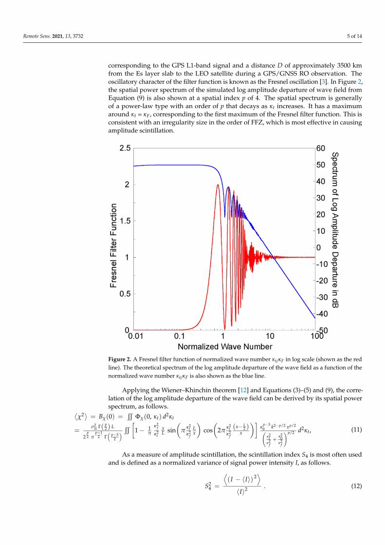
As described in the last section, the FFZ DF of a GPS RO observation on the Es layeris approximately 0.8 km. This means that a 50 Hz limb viewing setting can be used todetermine the complete scintillation index S4 and S2 values upon Es layer observation,but a 1 Hz limb viewing cannot. Figure 4 shows one example of FS3/COSMIC “atmPhs”(50-Hz) RO observation with an Es event recorded on 1 January 2007. As shown, significantamplitude fluctuations from L1-band signals were observed at E-region altitudes, andthe corresponding S4 and S2 altitudinal profiles can be derived by Equations (12) and(14) separately applied to a sliding window of 4 s amplitude data. However, the L2-bandsignals are much weaker and have insufficient sensitivity to derive reliable S4 and S2 valuesto be shown. Notably, there is strong scintillation in the Es event, and the peak S4 (S2) valueis 0.82 (0.39) for the GPS L1-band signals.

Remote Sens. 2021, 13, x FOR PEER REVIEW 8 of 15

3. Results The FS3/COSMIC is a joint Taiwan–U.S. mission consisting of six identical LEO mi-

cro-satellites from mid-2006 to 2019. Each spacecraft carried a GPS receiver developed by the Jet Propulsion Laboratory (JPL) and utilized four GPS antennas: two limb viewing occultation antennas remotely sensing the atmosphere and low ionosphere at 50 Hz from the Earth surface up to approximately 125 km, and two slant observing antennas for pre-cise orbit determination (POD) and remotely sensing the ionosphere at 1 Hz [23]. There-fore, the use of both limb viewing and POD antennas could produce simultaneous occul-tation observations consisting of two sets of 50 Hz and 1 Hz limb viewing links separately with different altitude resolutions of approximately 0.064 and 3.2 km at E-region altitudes. Both the GPS RO measurements include GPS and LEO satellite orbits, carrier excess phase and carrier signal–noise ratio (SNR) amplitudes for dual GPS L-band signals (f1 = 1575.42 MHz and f2 = 1227.60 MHz) at 50 Hz and 1 Hz, i.e., the “atmPhs” and “ionPhs” data, re-spectively. Notably, the FS3/COSMIC also provides 1 Hz amplitude scintillation S4 data at the L1 band as the “scnLv1” data. The amplitude scintillation measurements are per-formed by an on-board algorithm under a Gaussian distribution assumption applied to the raw 50 Hz L1-band SNR amplitude data (Syndergaard 2006, COSMIC S4 data, from the website: http://cdaac-www.cosmic.ucar.edu/cdaac/doc/documents/s4_descrip-tion.pdf, accessed on 22 August 2021). The on-board S4 measurements are not derived by the scintillation index definition shown in Equation (12), and are thus not discussed in this study.

As described in the last section, the FFZ DF of a GPS RO observation on the Es layer is approximately 0.8 km. This means that a 50 Hz limb viewing setting can be used to determine the complete scintillation index S4 and S2 values upon Es layer observation, but a 1 Hz limb viewing cannot. Figure 4 shows one example of FS3/COSMIC “atmPhs” (50-Hz) RO observation with an Es event recorded on 1 January 2007. As shown, significant amplitude fluctuations from L1-band signals were observed at E-region altitudes, and the corresponding S4 and S2 altitudinal profiles can be derived by Equations (12) and (14) sepa-rately applied to a sliding window of 4 s amplitude data. However, the L2-band signals are much weaker and have insufficient sensitivity to derive reliable S4 and S2 values to be shown. Notably, there is strong scintillation in the Es event, and the peak S4 (S2) value is 0.82 (0.39) for the GPS L1-band signals.

Figure 4. One example of FS3/COSMIC GPS RO observation with an Es event. The limb viewing L1- and L2-band SNR amplitudes of 50 Hz data versus GPS-LEO tangent point altitudes are shown in Figure 4. One example of FS3/COSMIC GPS RO observation with an Es event. The limb viewing L1-and L2-band SNR amplitudes of 50 Hz data versus GPS-LEO tangent point altitudes are shown inblack and gray, respectively. The resulting S4 and S2 altitudinal profiles of GPS L1-band signals arealso shown in blue and red, respectively. Notably, the peak S4 (S2) value is 0.82 (0.39).

As mentioned, 50 Hz GPS-LEO limb viewing has a vertical sampling spatial scaleof approximately 0.064 km, which is over one order less than the FFZ (~0.8 km) of theEs layer RO observation. We can perform de-sampling to obtain more sets of amplitudedata at different sampling frequencies of 50/n Hz, where n = 1, 2, . . . , 100. The resultingone hundred sets of amplitude data can be used to derive different altitudinal S4 and S4profiles using a 4 s sliding window, and obtain corresponding peak S4 and S2 values atsampling frequencies from 0.5 to 50 Hz, which are approximately equal to normalizedsampling spatial scales κs/κF of 0.2 to 20. Figure 5 shows the measured peaks S4, S2, andtheir ratio S2/S4 values as a function of κs/κF based on the FS3/COSMIC RO amplitudedata, as used in Figure 4. Notably, the measured peak S4 and S2 profiles in κs/κF fluctuatebut are mainly similar to the simulated S4 and S2 profiles in the strong scintillation caseof a complete S4 value of 0.8, as shown in Figure 3. The S4 and S2 values are saturated to~0.8 and ~0.4, respectively, when κs is larger than κF, and, when κs is less than κF, the S4

Remote Sens. 2021, 13, 3732 9 of 14

and S2 values decrease in general as the logarithm of κs decreases. Figure 5 also shows themeasured S2/S4 values to be more or less than 0.5 at different normalized sampling wavenumbers κs/κF from 0.2 to 20, i.e., the measured S2 values are also approximately half ofthe measured S4 values whenever κs is larger or less than κF.

Remote Sens. 2021, 13, x FOR PEER REVIEW 9 of 15

black and gray, respectively. The resulting S4 and S2 altitudinal profiles of GPS L1-band signals are also shown in blue and red, respectively. Notably, the peak S4 (S2) value is 0.82 (0.39).

As mentioned, 50 Hz GPS-LEO limb viewing has a vertical sampling spatial scale of approximately 0.064 km, which is over one order less than the FFZ (~0.8 km) of the Es layer RO observation. We can perform de-sampling to obtain more sets of amplitude data at different sampling frequencies of 50/n Hz, where n = 1, 2,..., 100. The resulting one hun-dred sets of amplitude data can be used to derive different altitudinal S4 and S4 profiles using a 4 s sliding window, and obtain corresponding peak S4 and S2 values at sampling frequencies from 0.5 to 50 Hz, which are approximately equal to normalized sampling spatial scales κs/κF of 0.2 to 20. Figure 5 shows the measured peaks S4, S2, and their ratio S2/S4 values as a function of κs/κF based on the FS3/COSMIC RO amplitude data, as used in Figure 4. Notably, the measured peak S4 and S2 profiles in κs/κF fluctuate but are mainly similar to the simulated S4 and S2 profiles in the strong scintillation case of a complete S4 value of 0.8, as shown in Figure 3. The S4 and S2 values are saturated to ~0.8 and ~0.4, respectively, when κs is larger than κF, and, when κs is less than κF, the S4 and S2 values decrease in general as the logarithm of κs decreases. Figure 5 also shows the measured S2/S4 values to be more or less than 0.5 at different normalized sampling wave numbers κs/κF from 0.2 to 20, i.e., the measured S2 values are also approximately half of the meas-ured S4 values whenever κs is larger or less than κF.

Figure 5. The dependence on normalized sampling wave number κs/κF for peak S4 (in black), S2 (in blue), and their ratio S2/S4 (in red). The experimental amplitude data are the same as those used in Figure 4.

The FS3/COSMIC program performed more than one thousand complete 50 Hz GPS RO E-region observations per day from mid-2006 to the end of 2016. There were more than two thousand complete E-region observations per day in the years from 2007 to 2009, but, after 2016, the RO observation number decreased to a few hundred per day in 2019. Ref. [11] determined that around 30% of those observations were Es events, based on the criteria of its peak S2 value (>0.2) and altitude (>80 km and less than the top altitude of each 50 Hz GPS RO observation). The local Es event occurrence rate could approach 70%

Figure 5. The dependence on normalized sampling wave number κs/κF for peak S4 (in black), S2

(in blue), and their ratio S2/S4 (in red). The experimental amplitude data are the same as those usedin Figure 4.

The FS3/COSMIC program performed more than one thousand complete 50 Hz GPSRO E-region observations per day from mid-2006 to the end of 2016. There were morethan two thousand complete E-region observations per day in the years from 2007 to 2009,but, after 2016, the RO observation number decreased to a few hundred per day in 2019.Ref. [11] determined that around 30% of those observations were Es events, based on thecriteria of its peak S2 value (>0.2) and altitude (>80 km and less than the top altitudeof each 50 Hz GPS RO observation). The local Es event occurrence rate could approach70% during hemispheric summer seasons. To determine the dependence on the samplingspatial scale of Es layer scintillation index determinations, the top, middle, and bottompanels of Figure 6 show the peak S4 and S2, and their S2/S4 ratio values, as a function ofthe normalized sampling wave number for three cases of strong scintillations (completeS4~0.8(±0.01) and 35 observations), moderate scintillations (complete S4~0.5(±0.01) and57 observations), and weak scintillations (complete S4~0.2(±0.01) and 143 observations),respectively. The experimental 50 Hz FS3/COSMIC data were obtained on 1 January and1 July 2007, and comprise 4750 GPS RO observations totally. Each RO observation wasde-sampled into one hundred sets of amplitude profiles used to derived correspondingpeak S4, S2, and S2/S4 values with different sampling frequencies from 0.5 to 50 Hz, i.e.,normalized sampling wave numbers κs/κF from approximately 0.2 to 20. Generally, asshown in Figure 6, there was a greater spread of peak S4, S2, and S2/S4 values whensampling wave number was less. This is reasonable, because the mean error increasesas its sampled number decreases, i.e., the sampling frequency decreases, and the same4 s sampling window is used. However, the dependence on sampling spatial scale ofthe S4, S2, and S2/S4 values is similar to that of the simulated S4, S2, and S2/S4 profiles,

Remote Sens. 2021, 13, 3732 10 of 14

shown in Figure 3, regardless of whether the scintillation cases are strong (complete S4~0.8),moderate (complete S4~0.5), or weak (complete S4~0.2).

Remote Sens. 2021, 13, x FOR PEER REVIEW 10 of 15

during hemispheric summer seasons. To determine the dependence on the sampling spa-tial scale of Es layer scintillation index determinations, the top, middle, and bottom panels of Figure 6 show the peak S4 and S2, and their S2/S4 ratio values, as a function of the normal-ized sampling wave number for three cases of strong scintillations (complete S4~0.8(±0.01) and 35 observations), moderate scintillations (complete S4~0.5(±0.01) and 57 observations), and weak scintillations (complete S4~0.2(±0.01) and 143 observations), respectively. The experimental 50 Hz FS3/COSMIC data were obtained on 1 January and 1 July 2007, and comprise 4750 GPS RO observations totally. Each RO observation was de-sampled into one hundred sets of amplitude profiles used to derived corresponding peak S4, S2, and S2/S4 values with different sampling frequencies from 0.5 to 50 Hz, i.e., normalized sam-pling wave numbers κs/κF from approximately 0.2 to 20. Generally, as shown in Figure 6, there was a greater spread of peak S4, S2, and S2/S4 values when sampling wave number was less. This is reasonable, because the mean error increases as its sampled number de-creases, i.e., the sampling frequency decreases, and the same 4 s sampling window is used. However, the dependence on sampling spatial scale of the S4, S2, and S2/S4 values is similar to that of the simulated S4, S2, and S2/S4 profiles, shown in Figure 3, regardless of whether the scintillation cases are strong (complete S4~0.8), moderate (complete S4~0.5), or weak (complete S4~0.2).

Remote Sens. 2021, 13, x FOR PEER REVIEW 11 of 15

Figure 6. Measured Es layer S4, S2, and their ratio S2/S4 values as a function of the normalized sam-pling wave number for three cases of strong scintillations (complete S4~0.8, top panel), moderate scintillations (complete S4~0.5, middle panel), and weak scintillations (complete S4~0.2, bottom panel). The experimental FS3/COSMIC data were obtained on 1 January and 1 July 2007.

4. Discussions Following the FS3/COSMIC mission, a follow-on program called FormoSat-7

(FS7)/COSMIC2 is in progress, with satellites launched on 25 June 2019. Similar to the FS3/COSMIC, the FS7/COSMIC2 is a six-LEO-satellite constellation mission orbiting at 24°

Figure 6. Cont.

Remote Sens. 2021, 13, 3732 11 of 14

Remote Sens. 2021, 13, x FOR PEER REVIEW 11 of 15

Figure 6. Measured Es layer S4, S2, and their ratio S2/S4 values as a function of the normalized sam-pling wave number for three cases of strong scintillations (complete S4~0.8, top panel), moderate scintillations (complete S4~0.5, middle panel), and weak scintillations (complete S4~0.2, bottom panel). The experimental FS3/COSMIC data were obtained on 1 January and 1 July 2007.

4. Discussions Following the FS3/COSMIC mission, a follow-on program called FormoSat-7

(FS7)/COSMIC2 is in progress, with satellites launched on 25 June 2019. Similar to the FS3/COSMIC, the FS7/COSMIC2 is a six-LEO-satellite constellation mission orbiting at 24°

Figure 6. Measured Es layer S4, S2, and their ratio S2/S4 values as a function of the normalizedsampling wave number for three cases of strong scintillations (complete S4~0.8, top panel), moderatescintillations (complete S4~0.5, middle panel), and weak scintillations (complete S4~0.2, bottompanel). The experimental FS3/COSMIC data were obtained on 1 January and 1 July 2007.

4. Discussions

Following the FS3/COSMIC mission, a follow-on program called FormoSat-7 (FS7)/COSMIC2 is in progress, with satellites launched on 25 June 2019. Similar to the FS3/COSMIC,the FS7/COSMIC2 is a six-LEO-satellite constellation mission orbiting at 24◦ inclinationand 520~720-km altitude. It enhances GNSS receiver capability to accommodate signalsfrom GPS and GLONASS satellites, and can provide more than 5000 RO observations perday within the region between geographic latitudes of ±40◦. The large dataset from theFS7/COSMIC2 program enables precise specifications and statistical studies on equatorialand low-latitude ionospheric electron densities and irregularities. Notably, each LEOsatellite of FS7/COSMIC2 also carries two limb viewing occultation antennas remotelysensing the atmosphere at 50 Hz, and another two slant observing antennas for PODand remotely sensing the ionosphere at 1 Hz. However, the altitude data of GPS/GNSSRO 50 Hz “atmPhs” are distributed between the Earth’s surface and a 60 km altitude,and do not include the E region range because of mission data storage constraints andsatellite downlink bandwidth limitations [24]. This means that Es layer observationsby FS7/COSMIC2 can be performed using 1 Hz “ionPhs” data only, and the S4 andS2 values derived by Equations (12) and (14) are underestimated under undersamplingconditions and are not complete. Therefore, it is necessary to find a method for solving theunderestimated scintillation indexes (S4 and S2).

To illustrate and compare the complete and undersampled scintillation observations,Figure 7 shows two scatter plots and the corresponding least-squares fitting lines for themeasured peak S4 and S2 values using 1 Hz FS3/COSMIC data versus the peak S4 and S2values measured using 50 Hz FS3/COSMIC data, respectively, on E and Es layer observa-tions. The experimental FS3/COSMIC data were recorded on 1 January and 1 July 2007,and the 1 Hz amplitudes have been de-sampled from the 50 Hz amplitudes of “atmPhs”data. The results show that the peak S4 (S2) measurements of E and Es layer observationsusing 50 Hz and de-sampled 1 Hz amplitude data have very high correlation coefficients

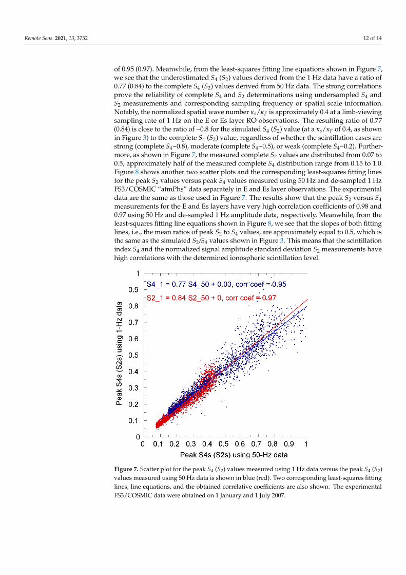
Remote Sens. 2021, 13, 3732 12 of 14

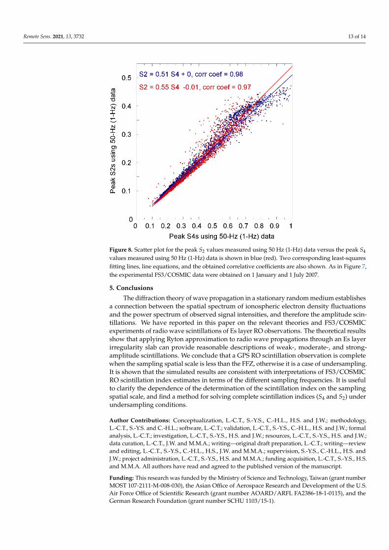
of 0.95 (0.97). Meanwhile, from the least-squares fitting line equations shown in Figure 7,we see that the underestimated S4 (S2) values derived from the 1 Hz data have a ratio of0.77 (0.84) to the complete S4 (S2) values derived from 50 Hz data. The strong correlationsprove the reliability of complete S4 and S2 determinations using undersampled S4 andS2 measurements and corresponding sampling frequency or spatial scale information.Notably, the normalized spatial wave number κs/κF is approximately 0.4 at a limb-viewingsampling rate of 1 Hz on the E or Es layer RO observations. The resulting ratio of 0.77(0.84) is close to the ratio of ~0.8 for the simulated S4 (S2) value (at a κs/κF of 0.4, as shownin Figure 3) to the complete S4 (S2) value, regardless of whether the scintillation cases arestrong (complete S4~0.8), moderate (complete S4~0.5), or weak (complete S4~0.2). Further-more, as shown in Figure 7, the measured complete S2 values are distributed from 0.07 to0.5, approximately half of the measured complete S4 distribution range from 0.15 to 1.0.Figure 8 shows another two scatter plots and the corresponding least-squares fitting linesfor the peak S2 values versus peak S4 values measured using 50 Hz and de-sampled 1 HzFS3/COSMIC “atmPhs” data separately in E and Es layer observations. The experimentaldata are the same as those used in Figure 7. The results show that the peak S2 versus S4measurements for the E and Es layers have very high correlation coefficients of 0.98 and0.97 using 50 Hz and de-sampled 1 Hz amplitude data, respectively. Meanwhile, from theleast-squares fitting line equations shown in Figure 8, we see that the slopes of both fittinglines, i.e., the mean ratios of peak S2 to S4 values, are approximately equal to 0.5, which isthe same as the simulated S2/S4 values shown in Figure 3. This means that the scintillationindex S4 and the normalized signal amplitude standard deviation S2 measurements havehigh correlations with the determined ionospheric scintillation level.

Remote Sens. 2021, 13, x FOR PEER REVIEW 13 of 15

Figure 7. Scatter plot for the peak S4 (S2) values measured using 1 Hz data versus the peak S4 (S2) values measured using 50 Hz data is shown in blue (red). Two correspond-ing least-squares fitting lines, line equations, and the obtained correlative coefficients are also shown. The experimental FS3/COSMIC data were obtained on 1 January and 1 July 2007.

Figure 8. Scatter plot for the peak S2 values measured using 50 Hz (1-Hz) data versus the peak S4 values measured using 50 Hz (1-Hz) data is shown in blue (red). Two corresponding least-squares

Figure 7. Scatter plot for the peak S4 (S2) values measured using 1 Hz data versus the peak S4 (S2)values measured using 50 Hz data is shown in blue (red). Two corresponding least-squares fittinglines, line equations, and the obtained correlative coefficients are also shown. The experimentalFS3/COSMIC data were obtained on 1 January and 1 July 2007.

Remote Sens. 2021, 13, 3732 13 of 14

Remote Sens. 2021, 13, x FOR PEER REVIEW 13 of 15

Figure 7. Scatter plot for the peak S4 (S2) values measured using 1 Hz data versus the peak S4 (S2) values measured using 50 Hz data is shown in blue (red). Two correspond-ing least-squares fitting lines, line equations, and the obtained correlative coefficients are also shown. The experimental FS3/COSMIC data were obtained on 1 January and 1 July 2007.

Figure 8. Scatter plot for the peak S2 values measured using 50 Hz (1-Hz) data versus the peak S4 values measured using 50 Hz (1-Hz) data is shown in blue (red). Two corresponding least-squares Figure 8. Scatter plot for the peak S2 values measured using 50 Hz (1-Hz) data versus the peak S4

values measured using 50 Hz (1-Hz) data is shown in blue (red). Two corresponding least-squaresfitting lines, line equations, and the obtained correlative coefficients are also shown. As in Figure 7,the experimental FS3/COSMIC data were obtained on 1 January and 1 July 2007.

5. Conclusions

The diffraction theory of wave propagation in a stationary random medium establishesa connection between the spatial spectrum of ionospheric electron density fluctuationsand the power spectrum of observed signal intensities, and therefore the amplitude scin-tillations. We have reported in this paper on the relevant theories and FS3/COSMICexperiments of radio wave scintillations of Es layer RO observations. The theoretical resultsshow that applying Ryton approximation to radio wave propagations through an Es layerirregularity slab can provide reasonable descriptions of weak-, moderate-, and strong-amplitude scintillations. We conclude that a GPS RO scintillation observation is completewhen the sampling spatial scale is less than the FFZ, otherwise it is a case of undersampling.It is shown that the simulated results are consistent with interpretations of FS3/COSMICRO scintillation index estimates in terms of the different sampling frequencies. It is usefulto clarify the dependence of the determination of the scintillation index on the samplingspatial scale, and find a method for solving complete scintillation indices (S4 and S2) underundersampling conditions.

Author Contributions: Conceptualization, L.-C.T., S.-Y.S., C.-H.L., H.S. and J.W.; methodology,L.-C.T., S.-Y.S. and C.-H.L.; software, L.-C.T.; validation, L.-C.T., S.-Y.S., C.-H.L., H.S. and J.W.; formalanalysis, L.-C.T.; investigation, L.-C.T., S.-Y.S., H.S. and J.W.; resources, L.-C.T., S.-Y.S., H.S. and J.W.;data curation, L.-C.T., J.W. and M.M.A.; writing—original draft preparation, L.-C.T.; writing—reviewand editing, L.-C.T., S.-Y.S., C.-H.L., H.S., J.W. and M.M.A.; supervision, S.-Y.S., C.-H.L., H.S. andJ.W.; project administration, L.-C.T., S.-Y.S., H.S. and M.M.A.; funding acquisition, L.-C.T., S.-Y.S., H.S.and M.M.A. All authors have read and agreed to the published version of the manuscript.

Funding: This research was funded by the Ministry of Science and Technology, Taiwan (grant numberMOST 107-2111-M-008-030), the Asian Office of Aerospace Research and Development of the U.S.Air Force Office of Scientific Research (grant number AOARD/ARFL FA2386-18-1-0115), and theGerman Research Foundation (grant number SCHU 1103/15-1).

Remote Sens. 2021, 13, 3732 14 of 14

Institutional Review Board Statement: Not applicable.

Informed Consent Statement: Not applicable.

Data Availability Statement: The FS3/COSMIC “atmPhs” data can be downloaded from the COS-MIC Data Analysis and Archive Center (CDAAC, http://cdaac-www.cosmic.ucar.edu/, accessedon 22 August 2021) and the Taiwan Analysis Center for COSMIC (TACC, http://tacc.cwb.gov.tw/cdaac/, accessed on 22 August 2021).

Acknowledgments: The work was possible thanks to a free access to FS3/COSMIC archives.

Conflicts of Interest: The authors declare no conflict of interest.

References1. Whitehead, J.D. Recent work on mid-latitude and equatorial sporadic E. J. Atmos. Terr. Phys. 1989, 51, 401–424. [CrossRef]2. Whitehead, J.D. Report on the production and prediction of Sporadic E. Rev. Geophys. Space Phys. 1970, 8, 65. [CrossRef]3. Yeh, K.C.; Liu, C.H. Radio wave scintillations in the ionosphere. Proc. IEEE 1982, 70, 324–360. [CrossRef]4. Mathews, J.D. Sporadic E: Current views and recent progress. J. Atmos. Solar-Terr. Phys. 1998, 60, 413–435. [CrossRef]5. Zeng, Z.; Sokolovskiy, S. Effect of sporadic E clouds on GPS radio occultation signals. Geophys. Res. Lett. 2010, 37,

L18817. [CrossRef]6. Ogawa, T.; Suzuki, A.; Kunitake, M. Spatial distribution of mid-latitude sporadic E scintillation in summer daytime. Radio Sci.

1989, 24, 527–538. [CrossRef]7. Hocke, K.; Igarashi, K.; Nakamura, M.; Wilkinson, P.; Wu, J.; Pavelyev, A.; Wickert, J. Global sounding of sporadic E layers by the

GPS/MET radio occultation experiment. J. Atmos. Solar-Terr. Phys. 2001, 63, 1973–1980. [CrossRef]8. Wu, D.L.; Ao, C.O.; Hajj, G.A.; Juarez, M.D.L.T.; Mannucci, A.J. Sporadic E morphology from GPS-CHAMP radio occultation. J.

Geophys. Res. 2005, 110, A01306. [CrossRef]9. Arras, C.; Wickert, J.; Beyerle, G.; Heise, S.; Schmidt, T.; Jacobi, C. A global climatology of ionospheric irregularities derived from

GPS radio occultation. Geophys. Res. Lett. 2008, 35, L14809. [CrossRef]10. Arras, C.; Wickert, J. Estimation of ionospheric sporadic E intensities from GPS radio occultation measurements. J. Atmos.

Solar-Terr. Phys. 2018, 171, 60–63. [CrossRef]11. Tsai, L.-C.; Su, S.-Y.; Liu, C.-H.; Schuh, H.; Wickert, J.; Alizadeh, M.M. Global morphology of ionospheric sporadic E layer from

the FormoSat-3/COSMIC GPS radio occultation experiment. GPS Solut. 2018, 22, 118. [CrossRef]12. Tatarskiı̌, V.I. The Effects of the Turbulent Atmosphere on Wave Propagation; National Technical Information Service: Springfield, VA,

USA, 1971.13. Crane, R.K. Spectra of ionospheric scintillation. J. Geophys. Res. 1976, 81, 2041–2050. [CrossRef]14. Rino, C.L. A power law phase screen model for ionospheric scintillation, 1. Weak scatter. Radio Sci. 1979, 14, 1135–1145. [CrossRef]15. Rino, C.L. A power law phase screen model for ionospheric scintillation, 2. Strong scatter. Radio Sci. 1979, 14,

1147–1155. [CrossRef]16. Priyadarshi, S. A review of ionospheric scintillation models. Surv. Geophys. 2015, 36, 295–324. [CrossRef]17. Shkarofsky, I.P. Generalized turbulence space-correlation and wave-number spectrum—Function pairs. Can. J. Phys. 1968, 46,

2133–2153. [CrossRef]18. Booker, H.G.; Ratcliffe, J.A.; Shinn, D.H. Diffraction from an irregular screen with applications to ionospheric problems. Philos.

Trans. Roy. Soc. London Ser. A 1950, 242, 579–607.19. Brown, W.P. Validity of the Ryton approximation. J. Opt. Soc. Amer. 1967, 57, 1539–1543. [CrossRef]20. Fried, D.L. Test of the Ryton approximation. J. Opt. Soc. Amer. 1967, 57, 268–269. [CrossRef]21. Wernik, A.W.; Liu, C.H. Application of the scintillation theory to ionospheric irregularities studies. Artif. Satell. 1975, 10, 37–58.22. Strangeways, H.J. Determining scintillation effects on GPS receivers. Radio Sci. 2009, 44, RS0A36. [CrossRef]23. Schreiner, W.; Rocken, C.; Sokolovskiy, S.; Syndergaard, S.; Hunt, D. Estimates of the precision of GPS radio occultation from the

COSMIC/FORMOSAT-3 mission. Geophys. Res. Lett. 2007, 34, L04808. [CrossRef]24. Schreiner, W.S.; Weiss, J.P.; Anthes, R.A.; Braun, J.; Chu, V.; Fong, J.; Hunt, D.; Kuo, Y.-H.; Meehan, T.; Serafino, W.; et al.

COSMIC-2 radio occultation constellation: First results. Geophys. Res. Lett. 2020, 47, e2019GL086841. [CrossRef]