Diagnostic Testing in Econometrics:

Variable Addition, RESET, and Fourier Approximations *

Linda F. DeBenedictis

and

David E. A. Giles

Policy, Planning and Legislation Branch,

Ministry of Social Services,

Victoria, B.C., CANADA

and

Department of Economics,

University of Victoria,

Victoria, B.C., CANADA

Revised, October 1996

(Published in A. Ullah & D.E.A. Giles (eds.), Handbook of Applied Economic Statistics,

Marcel Dekker, New York, 1998, pp. 383-417)

Author Contact: Professor David E. A. Giles, Department of Economics, University of

Victoria, P.O. Box 3050, MS 8532, Victoria, B.C., CANADA, V8W 3P5

FAX: +1-250-721 6214 Phone: +1-250-721 8540

e-mail: DGILES@UVIC.CA

2

I. INTRODUCTION

The consequences of model mis-specification in regression analysis can be severe in terms of the

adverse effects on the sampling properties of both estimators and tests. There are also

commensurate implications for forecasts and for other inferences that may be drawn from the

fitted model. Accordingly, the econometrics literature places a good deal of emphasis on

procedures for interrogating the quality of a model's specification. These procedures address the

assumptions that may have been made about the distribution of the model's error term, and they

also focus on the structural specification of the model, in terms of its functional form, the choice

of regressors, and possible measurement errors.

Much has been written about "diagnostic tests" for model mis-specification in econometrics in

recent years. The last two decades, in particular, have seen a surge of interest in this topic which

has, to a large degree, redressed what was previously an imbalance between the intellectual

effort directed towards pure estimation issues, and that directed towards testing issues of various

sorts. There is no doubt that diagnostic testing is now firmly established as a central topic in both

econometric theory and practice, in sympathy with Hendry (1980, p.403) urging that we should

"test, test and test". Some useful general references in this field include Krämer and Sonnberger

(1986), Godfrey (1988, 1996), and White (1994), among many others. As is discussed by Pagan

(1984), the majority of the statistical procedures that have been proposed for measuring the

inadequacy of econometric models can be allocated into one of two categories - "variable

addition" methods, and "variable transformation" methods. More than a decade later, it remains

the case that the first of these categories still provides a useful basis for discussing and

3

evaluating a wide range of the diagnostic tests that econometricians use. The equivalence

between variable addition tests and tests based on "Gauss-Newton regressions" is noted, for

instance, by Davidson and MacKinnon (1993, p.194), and essentially exploited by MacKinnon

and Magee (1990). Indeed it is the case that many diagnostic tests can be viewed and categorized

in more than one way.

In this paper we will be limiting our attention to diagnostic tests in econometrics which can be

classified as "variable addition" tests. This will serve to focus the discussion in a manageable

way. Pagan (1984) and Pagan and Hall (1983) provide an excellent discussion of this topic. Our

purpose here is to summarize some of the salient features of that literature and then to use it as a

vehicle for proposing a new variant of what is perhaps the best known variable addition test -

Ramsey's (1969) "Regression Specification Error (RESET) test".

The layout of the rest of the paper is as follows. In the next section we discuss some general

issues relating to the use of "variable addition" tests for model mis-specification. Section III

discusses the formulation of the standard RESET test, and the extent to which the distribution of

its statistic can be evaluated analytically. In section IV we introduce a modification of this test,

which we call the FRESET test (as it is based on a Fourier approximation) and we consider some

practical issues associated with its implementation. A comparative Monte Carlo experiment,

designed to explore the power of the FRESET test under (otherwise) standard conditions, is

described in section V; and section VI summarizes the associated results. The last section

contains some conclusions and recommendations which strongly favour the new FRESET test

over existing alternatives; and we note some work in progress which extends the present study

4

by considering the robustness of tests of this type to non-spherical errors in the data-generating

process.

II. VARIABLE ADDITION TESTS IN ECONOMETRICS

A. Preliminaries

One important theme that underlies many specification tests in econometrics is the idea that if a

model is correctly specified, then (typically) there are many weakly consistent estimators of the

model's parameters, and so the associated estimates should differ very little if the sample size is

sufficiently large. A substantial divergence of these estimates may be taken as a signal of some

sort of model mis-specification (e.g., White (1994, Ch.9)). Depending on the estimates which are

being compared, tests for various types of model mis-specification may be constructed. Indeed,

this basic idea underlies the well-known family of Hausman (1978) tests, and the information

matrix tests of White (1982, 1987). This approach to specification testing is based on the stance

that in practice, there is generally little information about the precise form of any mis-

specification in the model. Accordingly, no specific alternative specification is postulated, and a

pure significance test is used. This stands in contrast with testing procedures in which an explicit

alternative hypothesis is stated, and used in the construction and implementation of the test (even

though a rejection of the null hypothesis need not lead one to accept the stated alternative). In the

latter case, we frequently "nest" the null within the alternative specification, and then test

whether the associated parametric restrictions are consistent with the evidence in the data. The

use of Likelihood Ratio, Wald and Lagrange Multiplier tests, for example, in this situation are

common-place and well understood.

5

As noted above, specification tests which do not involve the formulation of a specific alternative

hypothesis are pure significance tests. They require the construction of a sample statistic whose

null distribution is known, at least approximately or asymptotically. This statistic is then used to

test the consistency of the null with the sample evidence. In the following discussion we will

encounter tests which involve a specific alternative hypothesis, although the latter may involve

the use of proxy variables to allow for uncertainties in the alternative specification. Our

subsequent focus on the RESET test involves a procedure which really falls somewhere between

these two categories, in that although a specific alternative hypothesis is formulated, it is largely

a device to facilitate a test of a null specification. Accordingly, it should be kept in mind that the

test is essentially a "destructive" one, rather than a "constructive" one, in the sense that a

rejection of the null hypothesis (and hence of the model's specification) generally will not

suggest any specific way of re-formulating the model in a satisfactory form. This is certainly a

limitation on its usefulness, so it is all the more important that it should have good power

properties. If the null specification is to be rejected, with minimal direction as to how the model

should be re-specified, then at least one would hope that we are rejecting for the right reason(s).

Accordingly, in our re-consideration of the RESET test in Sections III and IV below we

emphasize power properties in a range of circumstances.

Variable addition tests are based on the idea that if the model specification is "complete", then

additions to the model should have an insignificant impact, in some sense. As is noted by Pagan

and Hall (1983) and Pagan (1984), there are many forms that such additions can take. For

6

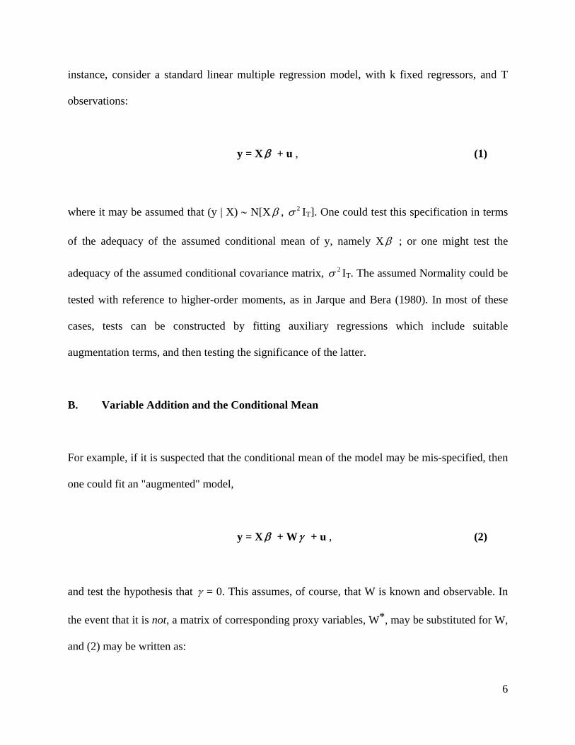
instance, consider a standard linear multiple regression model, with k fixed regressors, and T

observations:

y = X + u , (1)

where it may be assumed that (y | X) N[X , 2 IT]. One could test this specification in terms

of the adequacy of the assumed conditional mean of y, namely X ; or one might test the

adequacy of the assumed conditional covariance matrix, 2 IT. The assumed Normality could be

tested with reference to higher-order moments, as in Jarque and Bera (1980). In most of these

cases, tests can be constructed by fitting auxiliary regressions which include suitable

augmentation terms, and then testing the significance of the latter.

B. Variable Addition and the Conditional Mean

For example, if it is suspected that the conditional mean of the model may be mis-specified, then

one could fit an "augmented" model,

y = X + W + u , (2)

and test the hypothesis that = 0. This assumes, of course, that W is known and observable. In

the event that it is not, a matrix of corresponding proxy variables, W*, may be substituted for W,

and (2) may be written as:

7

y = X + W* + (W - W*) + u = X + W* + e , (3)

and we could again test if = 0. As Pagan (1984, p. 106) notes, the effect of this substitution

will show up in terms of the power of the test that is being performed. An alternative way of

viewing (2) (or (3) if the appropriate substitution of the proxy variables is made below) is by

way of an auxiliary regression with residuals from (2.1) as the dependent variable:

(y - Xb) = X( - b) + W + u , (4)

where b = (X'X)-1X'y is the least squares estimator of in (1). This last model is identical to (2)

and the test of = 0 will yield an identical answer in each case. However, (4) emphasises the

role of diagnostic tests in terms of explaining residual values.

The choice of W (or W*) will be determined by the particular way in which the researcher

suspects that the conditional mean of the basic model may be mis-specified. Obvious situations

that will be of interest include a wrongly specified functional form for the model, or terms that

have been omitted wrongly from the set of explanatory variables. There is, of course, a natural

connection between these two types of model mis-specification, as we discuss further below. In

addition, tests of serial independence of the errors, structural stability, exogeneity of the

regressors, and those which discriminate between non-nested models, can all be expressed as

variable-addition tests which focus on the conditional mean of the data-generating process. All

of these situations are discussed in some detail by Pagan (1984). Accordingly, we will simply

8

summarize some of the salient points here, and we will focus particularly on functional form and

omitted effects, as these are associated most directly with the RESET test and hence with the

primary focus of this paper.

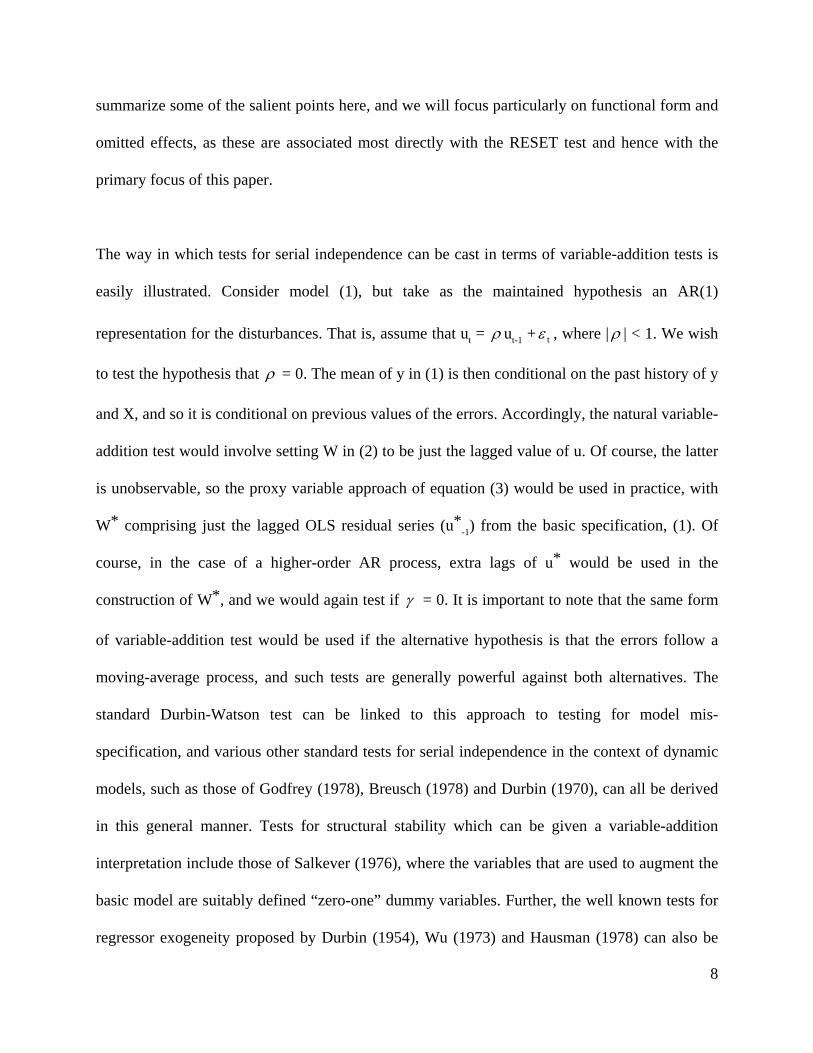
The way in which tests for serial independence can be cast in terms of variable-addition tests is

easily illustrated. Consider model (1), but take as the maintained hypothesis an AR(1)

representation for the disturbances. That is, assume that ut = ut-1 + t , where | | < 1. We wish

to test the hypothesis that = 0. The mean of y in (1) is then conditional on the past history of y

and X, and so it is conditional on previous values of the errors. Accordingly, the natural variable-

addition test would involve setting W in (2) to be just the lagged value of u. Of course, the latter

is unobservable, so the proxy variable approach of equation (3) would be used in practice, with

W* comprising just the lagged OLS residual series (u*-1) from the basic specification, (1). Of

course, in the case of a higher-order AR process, extra lags of u* would be used in the

construction of W*, and we would again test if = 0. It is important to note that the same form

of variable-addition test would be used if the alternative hypothesis is that the errors follow a

moving-average process, and such tests are generally powerful against both alternatives. The

standard Durbin-Watson test can be linked to this approach to testing for model mis-

specification, and various other standard tests for serial independence in the context of dynamic

models, such as those of Godfrey (1978), Breusch (1978) and Durbin (1970), can all be derived

in this general manner. Tests for structural stability which can be given a variable-addition

interpretation include those of Salkever (1976), where the variables that are used to augment the

basic model are suitably defined “zero-one” dummy variables. Further, the well known tests for

regressor exogeneity proposed by Durbin (1954), Wu (1973) and Hausman (1978) can also be

9

re-expressed as variable-addition tests which use appropriate instrumental variables in the

construction of the proxy matrix, W* (e.g., Pagan (1984, pp.114-115)).

The problem of testing between (non-nested) models is one which has attracted considerable

attention during the last twenty years, e.g., McAleer (1987, 1995). Such tests frequently can be

interpreted as variable-addition tests which focus on the specification of the conditional mean of

the model. By way of illustration, recall that in model (1) the conditional mean of y (given X,

and the past history of the regressors and of y) is X . Suppose that there is a competing model

for explaining y, with a conditional mean of X+ , where X and X+ are non-nested, and is a

conformable vector of unknown parameters. To test one specification of the model against the

other, there are various ways of applying the variable-addition principle. One obvious possibility

(assuming an adequate number of degrees of freedom) would be to assign W*=X+ in (3), and

then apply a conventional F-test. This is the approach suggested by Pesaran (1974) in one of the

earlier contributions to this aspect of the econometrics literature. Another possibility, which is

less demanding on degrees of freedom, is to set W* = X+(X+'X+)-1X+'y (that is, using the OLS

estimate of the conditional mean from the second model as the proxy variable), which gives us

the J-test of Davidson and MacKinnon (1981). There have been numerous variants on the latter

theme, as is discussed by McAleer (1987), largely with the intention of improving the small-

sample powers of the associated variable-addition tests.

Our main concern in this paper is with variable-addition tests which address possible mis-

specification of the functional form of the model, or the omission of relevant explanatory effects.

The treatment of the latter issue fits naturally into the framework of equations (1) - (4). The key

10

decision that has to be made in order to implement a variable-addition test in this case is the

choice of W (or, more likely, W*). If we have some idea what effects may have been omitted

wrongly, then this determines the choice of the "additional" variables, and if we were to make a

perfect choice then the usual F-test of = 0 would be exact, and Uniformly Most Powerful

(UMP). Of course, this really misses the entire point of our present discussion, which is based on

the premise that we have specified the model to the best of our knowledge and ability, but are

still concerned that there may be some further, unknown, omitted effects. In this case, some

ingenuity may be required in the construction of W or W*, which is what makes the RESET test

(and our modification of this procedure in this paper) of particular interest. Rather than develop

this point further here, we leave a more detailed discussion of the RESET test to section III

below.

In many cases, testing the basic model for a possible mis-specification of its functional form can

be considered in terms of testing for omitted effects in the conditional mean. This is trivially

clear if, for example, the fitted model includes simply a regressor, xt, but the correct specification

involves a polynomial in xt. Constructing W* with columns made up of powers of xt would

provide an optimal test in his case. Similarly, if the fitted model included xt as a regressor, but

the correct specification involved some (observable) transformation of xt, such as log(xt), then

(2) could be constructed so as to include both the regressor and its transformation, and the

significance of the latter could be tested in the usual way. Again, of course, this would be

feasible only if one had some prior information about the likely nature of the mis-specification of

the functional form. (See also, Godfrey, McAleer and McKenzie (1988)).

11

More generally, suppose that model (1) is being considered, but in fact the correct specification

is

y = f (X, 1 , 2 ) + u , (5)

where f is a non-linear function which is continuously differentiable with respect to the

parameter sub-vector, 2 . If (1) is nested within (5) by setting 2 = 20 , then by taking a Taylor

series expansion of f about the (vector) point 20 , we can (after some re-arrangement) represent

(5) by a model which is of the form (3), and then proceed in the usual way to test (1) against (5)

by testing if = 0 via a RESET test. More specifically, this can be achieved, to a first-order

approximation, by setting

W* = f [X, b1 , 20 ] / 2 ; = ( 2 - 2

0 ) , (6)

where b1 is the least squares estimator of the sub-vector 1 , obtained subject to the restriction

that 2 = 20 . As we will see again in section III below, although the presence of b1 makes W*

random, the usual F-test of = 0 is still valid, as a consequence of the Milliken-Graybill (1970)

Theorem.

As we have seen, many tests of model mis-specification can be formulated as variable-addition

tests in which attention focuses on the conditional mean of the underlying data-generating

process. This provides a very useful basis for assessing the sampling properties of such tests.

12

Model (3) above forms the basis of the particular specification test (the RESET test) that we will

be considering in detail later in this paper. Essentially, we will be concerned with obtaining a

matrix of proxy variables, W*, that better represents an arbitrary form of mis-specification than

do the usual choices of this matrix. In this manner, we hope to improve on the ability of such

tests to reject models which are falsely specified in the form of equation (1).

C. Variable Addition and Higher Moments

Although our primary interest in this paper is with variable-addition tests which focus on mis-

specification relating to the conditional mean of the model, some brief comments are in order

with respect to related tests which focus on the conditional variance and on higher order

moments. Of the latter, only the third and fourth moments have been considered traditionally in

the context of variable-addition tests, as the basis of testing the assumption of Normally

distributed disturbances (e.g., Jarque and Bera (1987)). Tests which deal with the conditional

variance of the underlying process have been considered in a variable-addition format by a

number of authors.

Essentially, the assumption that the variance, 2 , of the error term in (1) is a constant is

addressed by considering alternative formulations, such as :

t2 = 2 + zt , (7)

13

where zt is an observation on a vector of r known variables, and is (r × 1). We then test the

hypothesis that = 0. To make this test operational, equation (7) needs to be re-formulated as a

"regression relationship" with an observable "dependent variable", and a stochastic "error term".

The squared t'th element of u in (1) gives us t2 , on average, so it is natural to use the

corresponding squared OLS residuals, on the left hand side of (7). Then, we have:

(u*t)

2 = 2 + zt + (u*t)

2 - t2 = 2 + zt + vt , (8)

where vt = (u*t)

2 - t2 . Equation (8) can be estimated by OLS to give estimates of 2 and , and

to provide a natural test of = 0. The (asymptotic) legitimacy of the usual t-test (or F-test) in

this capacity is established, for example, by Amemiya (1977).

So, the approach in (8) is essentially analogous to the variable-addition approach in the case of

equation (2) for the conditional mean of the model. As was the situation there, in practice we

might not be able to measure the zt vector, and a replacement proxy vector, z*t might be used

instead. Then the counterpart to equation (3) would be:

14

(u*t)

2 = 2 + zt + (zt - z*

t) + vt = 2 + z*t + v*

t , (9)

where we again test if = 0, and the choice of z*t determines the particular form of

heteroskedasticity against which we are testing.

For example, if z* is an appropriately defined scalar dummy variable then we can test against a

single break in the value of the error variance at a known point. This same idea also relates to the

more general homoskedasticity tests of Harrison and McCabe (1979) and Breusch and Pagan

(1979). Similarly, Garbade's (1977) test for systematic structural change can be expressed as the

above type of variable-addition test, with z*t = t xt

2 ; and Engle's (1982) test against ARCH(1)

errors amounts to a variable addition test with z*t = (u*

t-1)2. Higher order ARCH and GARCH

processes1 can be accommodated by including additional lags of (u*t)

2 in the definition of z*.

Pagan (1984, pp.115-118) provides further details as well as other examples of specification tests

which can be given a variable-addition interpretation with respect to the conditional variance of

the errors.

D. Multiple Testing

Variable addition tests have an important distributional characteristic which we have not yet

discussed. To see this, first note that under the assumptions of model (1), the UMP test of = 0

will be a standard F-test if X and W (or W*) are both non-stochastic and of full column rank. In

the event that either the original or "additional" regressors are stochastic (and correlated with the

errors), and/or the errors are non-Normal, the usual F-statistic for testing if = 0 can be scaled

15

to form a statistic which will be asymptotically Chi-square. More specifically, if there are T

observations and if rank(X) = k and rank(W) = p, then the usual F statistic will be Fp, , under the

null (where = T-k-p). Then (pF) will be asymptotically p2 under the null2. Now, suppose

that we test the model's specification by means of a variable addition test based on (2), and

denote the usual test statistic by Fw. Then, suppose we consider a second test for mis-

specification by fitting the "augmented" model,

y = X + Z + v , (10)

where rank(Z) = q, say. In the latter case, denote the statistic for testing if = 0 by Fz.

Asymptotically, (pFw) is p2 , and (qFz) is q

2 , under the respective null hypotheses.

Now, from the usual properties of independent Chi square statistics, we know that if the above

two tests are independent, then (pFw + qFz) is asymptotically p+q2 under the null that = =

0. As is discussed by Bera and McKenzie (1987) and Eastwood and Godfrey (1992, p.120),

independence of the tests requires that plim (Z'W/T) = 0, and that either plim (Z'X/T) = 0, or

plim (W'X/T) = 0. The advantages of this are the following. First, if these variable addition

specification tests are applied in the context of (2) and (10) sequentially, then the overall

significance level can be controlled. Specifically, if the (asymptotic) significance levels for these

two separate tests are set at w and z respectively, then3 the overall joint significance level

will be [1 - (1 - w )(1 - z )]. Second, the need to fit a "super-model", which includes all of the

(distinct) columns of X, W and Z as regressors, can be avoided. The extension of these ideas to

16

testing sub-sets of the regressors is discussed in detail by Eastwood and Godfrey (1992, pp.120-

122).

A somewhat related independence issue also arises in the context of certain variable addition

tests, especially when the two tests in question focus on different moments of the underlying

stochastic process. Consider, for example, tests of the type discussed in section II.B above.

These deal with the first moment of the distribution and are simply tests of exact restrictions on a

certain regression coefficient vector. Now, suppose that we also wanted to test for a shift in the

variance of the error term in the model, perhaps at some known point(s) in the sample. It is well

known4 that many tests of the latter type (e.g., those of Goldfeld and Quandt (1965), Harrison

and McCabe (1979) and Breusch and Pagan (1979)) are independent (at least asymptotically in

some cases) of the usual test for exact restrictions on the regression coefficients. Once again, this

eases the task of controlling the overall significance level, if we are testing for two types of

model mis-specification concurrently, but do not wish to construct "omnibus tests".

The discussion above assumes, implicitly, that the two (or more) variable addition tests in

question are not only independent, but also that they are applied separately, but "concurrently".

By the latter, we mean that each individual test is applied regardless of the outcome(s) of the

other test(s). That is, we are abstracting from any "pre-test testing" issues. Of course, in practice,

this may be too strong an assumption. A particular variable addition test (such as the RESET

test) which relates to the specification of the conditional mean of the model might be applied

only if the model "passes" another (separate and perhaps independent) test of the specification of

the conditional variance of the model. If it fails the latter test, then a different variable addition

17

test for the specification of the mean may be appropriate. That is, the choice of the form of one

test may be contingent on the outcome of a prior test of a different feature of the model's

specification. Even if the first-stage and second-stage tests are independent, there remains a "pre-

testing problem" of substance5. The true significance level of the two-part test for the

specification of the conditional mean of the model will differ from the sizes nominally assigned

to either of its component parts, because of the randomization of the choice of second-stage test

which results from the application of the first-stage test (for the specification of the conditional

variance of the model).

More generally, specification tests of the variable-addition type may not be independent of each

other. As is noted by Pagan (1984, pp. 125-127), it is unusual for tests which focus on the same

conditional moment to be mutually independent. One is more likely to encounter such

independence between tests which relate to different moments of the underlying process (as in

the discussion above). In such cases there are essentially two options open. The first is to

construct joint variable-addition tests of the various forms of mis-specification that are of

interest. This may be a somewhat daunting task, and although some progress along these lines

has been made (e.g., Bera and Jarque (1982)), there is still little allowance for this in the standard

econometrics computer packages. The second option is to apply separate variable-addition tests

for the individual types of model mis-specification, and then adopt an "induced testing strategy"

by rejecting the model if at least one of the individual test statistics is significant. Generally, in

view of the associated non-independence and the likely complexity of the joint distribution of the

individual test statistics, the best that one can do is to compute bounds on the overall significance

level for the "induced test". The standard approach in this case would be to use Bonferroni

18

inequalities (e.g., David (1981) and Schwager (1984)), though generally such bounds may be

quite wide, and hence relatively uninformative. A brief discussion of some related issues is given

by Krämer and Sonnberger (1986, pp. 147-155), and Savin (1984) deals specifically with the

relationship between multiple t-tests and the F-test. This, of course, is directly relevant to the

case of certain variable-addition tests for the specification of the model's conditional mean.

E. Other Distributional Issues

There are several further distributional issues which are important in the context of variable-

addition tests. In view of our subsequent emphasis on the RESET test in this paper, it is

convenient and appropriate to explore these issues briefly in the context of tests which focus on

the conditional mean of the model. However, it should be recognized that the general points that

are made in the rest of this section also apply to variable-addition tests relating to other moments

of the data-generating process. Under our earlier assumptions, the basic form of the test in which

we are now interested is an F-test of = 0 in the context of model (2). In that model, if W is

truly the precise representation of the omitted effects, then the F-test will be UMP. Working,

instead, with the matrix of proxy variables, W*, as in (3), does not affect the null distribution of

the test statistic in general, but it does affect the power of the test, of course. Indeed, the

reduction in power associated with the use of the proxy variables increases as the correlations

between the columns of W and those of W* decrease. Ohtani and Giles (1993) provide some

exact results relating to this phenomenon under very general distributional assumptions, and find

the reduction in power to be more pronounced as the error distribution departs from Normality.

They also show that, regardless of the degree of non-normality, the test can be biased6 as the

19

hypothesis error grows, and they prove that the usual null distribution for the F-statistic for

testing if = 0 still holds even under these more general conditions.

Of course, in practice, the whole point of the analysis is that the existence, form and degree of

model mis-specification are unknown. Although the general form of W* will be chosen to reflect

the type of mis-specification against which one is testing, the extent to which W* is a "good"

proxy for W (and hence for the omitted effect) will not be able to be determined exactly. This

being the case, in general it is difficult to make specific statements about the power of such

variable-addition tests. As long as W* is correlated with W (asymptotically), a variable addition

test based on model (3) will be consistent. That is, for a given degree of specification error, as

the sample size grows the power of the test will approach unity. In view of the immediately

preceding comments, the convergence path will depend on the forms of both W and W*.

The essential consistency of a basic variable-addition test of = 0 in (2) is readily established.

Following Eastwood and Godfrey (1992, pp.123-125), and assuming that (X'X), (W'W) and

(X'W) are each Op(T), the consistency of a test based on Fw (as defined in section II.D, and

assuming independent and homoskedastic disturbances) is assured if plim (Fw / T) 0 under the

alternative. Now, as is well known, we can write

Fw = [(RSS - USS) / p] / [USS / (T-k-p)] , (11)

where RSS denotes the sum of the squared residuals when (2) is estimated by OLS subject to the

restriction that = 0, and USS denotes the corresponding sum of squares when (2) is estimated

20

by unrestricted OLS. Under quite weak conditions the denominator in (11) converges in

probability to 2 (by Khintchine's Theorem). So, by Slutsky's Theorem, in order to show that

the test is consistent, it is sufficient to establish that plim [(RSS - USS) / T] 0 under the

alternative7. Now, for our particular problem we can write

[(RSS - USS) / T] = '[R (X*'X* / T)-1 R']-1 , (12)

where R = [Ik , 0p], and X* = (X : W). Given our assumption above about the orders in

probability of the data matrices, we can write plim (X*'X* / T) = Q*, say, where Q* is finite and

non-singular. Then, it follows immediately from (12) that plim [(RSS - USS) / T] > 0, if 0,

and so the test is consistent. It is now clear why consistency is retained if W* is substituted for

W, as long as these two matrices are asymptotically correlated. It is also clear that this result will

still hold even if W is random or if W* is random (as in the case of a RESET test involving some

function of the OLS prediction vector from (1) in the construction of W*).

Godfrey (1988, pp.102-106) discusses another important issue that arises in this context, and

which is highly pertinent for our own analysis of the RESET test in this paper. In general, if we

test one of the specifications in (2) - (4) against model (1), by testing if = 0, it is likely that in

fact the true data-generating process differs from both the null and maintained hypotheses. That

is, we will generally be testing against an incorrect alternative specification. In such cases, the

determination of even the asymptotic power of the usual F-test (or its large-sample Chi square

counterpart) is not straightforward, and is best approached by considering a sequence of local

21

alternatives. Not surprisingly, it turns out that the asymptotic power of the test depends on the

(unknown) extent to which the maintained model differs from the true data-generating process.

Of course, in practice the errors in the model may be serially correlated and/or heteroskedastic,

in which case variable addition tests of this type generally will be inconsistent, and their power

properties need to be considered afresh in either large or small samples. Early work by Thursby

(1979, 1982) suggested that the RESET test might be robust to autocorrelated errors, but as is

noted by Pagan (1984, p.127), and explored by Porter and Kashyap (1984), this is clearly not the

case. We abstract from this situation in the development of a new version of the RESET test later

in this paper, but it is a topic that is being dealt with in some detail in our current research.

Finally, we should keep in mind that a consistent test need not necessarily have high power in

small samples, and so this remains an issue of substance when considering specific variable-

addition tests.

Finally, it is worth commenting on the problem of discriminating between two or more variable-

addition tests, each of which is consistent in the sense described above. If the significance level

for the tests is fixed (as opposed to being allowed to decrease as the sample size increases) then

there are at least two fairly standard ways of dealing with this issue. These involve bounding the

powers of the tests away from unity as the sample size grows without limit. The first approach is

to use the "approximate slope" analysis of Bahadur (1960, 1967). This amounts to determining

how the asymptotic significance level of the test must be reduced if the power of the test is to be

held constant under some fixed alternative. The test statistics are Op(T), and they are compared

against critical values which increase with T. The approximate slope for a test statistic, S, which

22

is asymptotically Chi square, is just8 plim (S/T). This is the same quantity that we considered

above in the determination of the consistency of such a test. A choice between two consistent

tests which test the same null against the same alternative can be made by selecting so as to

maximize the approximate slope. Of course, once again this does not guarantee good power

properties in small samples.

A second approach which may be used to discriminate between consistent tests is to consider a

sequence of local alternatives. In this approach, the alternative hypothesis is adjusted so that it

approaches the null hypothesis in a manner that ensures that the test statistics are Op(1). Then, a

fixed critical value can be used, and the asymptotic powers of the tests that can be compared as

they will each be less than unity. In our discussion of the traditional RESET test in the next

section, and of a new variant of this test in section IV, neither of the above approaches to

discriminating between consistent tests are particularly helpful. There, the tests that are being

compared have the same algebraic construction, but they differ in terms of the number of

columns in W* and the way in which these columns are constructed from the OLS prediction

vector associated with the basic model. In general, the "approximate slope" and "local

alternatives" approaches do not provide tractable expressions upon which to base clear

comparisons in this case. However, in practical terms our interest lies in the small-sample

properties of the tests, and it is on this characteristic that we focus below.

III. THE RESET TEST

23

Among the many "diagnostic tests" that econometricians routinely use, some variant or other of

the RESET test is widely employed to test for a non-zero mean of the error term. That is, it tests

implicitly whether a regression model is correctly specified in terms of the regressors that have

been included. Among the reasons for the popularity of this test are the fact that it is easily

implemented, and the fact that it is an exact test, whose statistic follows an F-distribution under

the null. The construction of the test does, however, require a choice to be made over the nature

of certain "augmenting regressors" that are employed to model the mis-specification, as we saw

in section II.B. Depending on this choice, the RESET test statistic has a non-null distribution

which may be doubly non-central F, or may be totally non-standard. Although this has no

bearing on the size of the test, it has obvious implications for its power.

The most common construction of the RESET test involves augmenting the regression of interest

with powers of the prediction vector from a least squares regression of the original specification,

and testing their joint significance. As a result of the Monte Carlo evidence provided by Ramsey

and Gilbert (1972) and Thursby (1989), for example, it is common for the second, third and

fourth powers of the prediction vector to be used in this way.9 Essentially, Ramsey's original

suggestion, following earlier work by Anscombe (1961), involves approximating the unknown

non-zero mean of the errors, which reflects the extent of the model mis-specification, by some

analytic function of the conditional mean of the model. The specific construction of the RESET

test noted above then invokes a polynomial approximation, with the least squares estimator of

the conditional mean replacing its true counterpart.

24

Other possibilities include using powers and/or cross-products of the individual regressors,

rather than powers of the prediction vector, to form the augmenting terms. Thursby and Schmidt

(1977) provide simulation results which appear to favour this approach. However, all of the

variants of the RESET test that have been proposed to date appear to rely on the use of local

approximations, essentially of a Taylor series type, of the conditional mean of the regression.

Intuitively, there may be gains in terms of the test's performance if a global approximation were

used instead. This paper pursues this intuition by suggesting the use of an (essentially unbiased)

Fourier flexible approximation. This suggestion captures the spirit of the development of cost

and production function modelling, and the associated transition from polynomial functions (e.g.,

Johnston (1960)), to Translog functions (e.g., Christensen et al. (1971, 1973)), and then to

Fourier functional forms (e.g., Gallant (1981) and Mitchell and Onvural (1995, 1996)).

Although Ramsey (1969) proposed a "battery" of specification tests for the linear regression

model, with the passage of time and the associated development of the testing literature, the

RESET test is the one which has survived. Ramsey's original discussion was based on the use of

Theil's (1965, 1968) "BLUS" residuals, but the analysis was subsequently re-cast in terms of the

usual Ordinary Least Squares (OLS) residuals (e.g., Ramsey and Schmidt (1976), Ramsey

(1983)), and we will follow the latter convention in this paper. As Godfrey (1988, p.106)

emphasises, one of the principles which underlies the RESET test is that the researcher has only

the same amount of information available when testing the specification of a regression model as

was available when the model was originally formulated and estimated. Accordingly direct tests

against new theories, perhaps embodying additional variables, are ruled out.

25

A convenient way of discussing and implementing the standard RESET test is as follows.

Suppose that the regression model under consideration is (2.1), which we reproduce here:

y = X + u , (13)

where X is (T×k), of rank k, and non-stochastic; and it is assumed that u N[0, 2 IT]. Such a

model would be "correctly specified". Now, suppose that we allow for the possibility that the

model is mis-specified through the omission of relevant regressors or the wrong choice of

functional form. In this case, E[u | X] = 0. The basis of the RESET test is to approximate

by Z , which corresponds to W* in (2.3), and fit an augmented model,

y = X + Z + . (14)

We then test if = 0, by testing if = 0, using the usual "F test" for restrictions on a subset of

the regression coefficients. Different choices of the [T×p] matrix Z lead to different variants of

the RESET test. As noted above, the most common choice is to construct Z to have t'th. row

vector,

Zt = [(Xb)t2, (Xb)t

3, ....., (Xb)tp+1] , (15)

where often p = 3; b = (X'X)-1X'y is the OLS estimator of from (1); and (Xb)t is therefore the

t'th. element of the associated prediction vector, y = Xb.

26

If Z is chosen in this way (or if it is non-random, or if it depends on y only through b), then, as a

consequence of the Milliken-Graybill (1970) Theorem, the RESET test statistic is F-distributed

with p and (T-k-p) degrees of freedom under the null that = 0,10 provided that the disturbances

are NID (0, 2 ). If Z is non-stochastic (as would be the case if Thursby and Schmidt's (1977)

proposal, of using powers of the regressors to augment the model, were followed) then the test

statistic's non-null distribution is doubly non-central F with the same degrees of freedom11, and

with numerator and denominator non-centrality parameters,

1 = MX Z (Z' MX Z)-1 Z' MX 2 (16)

2 = [MX - MXZ (Z' MX Z)-1 Z' MX ] 2 . (17)

In this case, the power of the RESET test can be computed exactly, for any given degree of mis-

specification, , by recognizing that

Pr.[F(p, T-k-p; 1 , 2 ) c] = Pr.[(1/p) 2 (p; 1 ) - (c/(T-k-p)) 2 (T-k-p; 2 )0] , (18)

where "F" denotes a doubly non-central F-statistic, and 2 denotes a non-central Chi-square

statistic, each with degrees of freedom and non-centrality parameters as shown. The algorithm of

Davies (1980), which is conveniently coded in the SHAZAM (1993) package, provides an

27

efficient and accurate means of computing such probabilities, although we are not aware of any

studies which do this in the context of the RESET test.

If, as is generally the case in practice, Z is constructed from powers of Xb, or is random for any

other reason, then 1 and 2 will be random, and the non-null distribution of the RESET test

statistic will no longer be doubly non-central F. The power characteristics associated with its

non-standard distribution will depend on the specific choice of Z (and hence on the number of

powers of Xb that may be used, if this choice is adopted), and are then best explored via Monte

Carlo simulation. This is the approach that we adopt in this paper.

28

IV. FOURIER APPROXIMATIONS AND THE FRESET TEST

As was noted above, the essence of Ramsey's RESET test is to approximate the unknown by

some analytic function of X (or, more precisely, of the observable y = Xb). A power series

approximation is one obvious possibility, but there are other approximations which may be more

attractive. In particular, as Gallant (1981) has argued in a different context, one weakness of

Taylor series approximations (which include the power series and Translog approximations, for

example) is that they have only local validity. Taylor's Theorem is valid only on a

neighbourhood of some unspecified size containing a specific value of the argument of the

function to be approximated. On the other hand, a Fourier approximation has global validity.

Such approximations can take the form of a conventional sine/cosine expansion, or the less

conventional Jacobi, Laguerre or Hermite expansions. In this paper we consider using a

sine/cosine expansion of Xb to approximate12 . Although Gallant (1981) has suggested that the

precision of a truncated Fourier series can generally be improved by adding a second-order

Taylor series approximation (see also Mitchell and Onvural (1995)), we do not pursue this

refinement in the present study.

In order to obtain a Fourier representation of Z in (14), and hence a Fourier approximation of

the unknown , by using Xb, we need to first transform the elements of this vector to lie in an

interval of length 2 , such as [- , + ]. This is because a Fourier representation is defined

only if the domain of the function is in an interval of length 2 . Mitchell and Onvural (1995,

1996), and other authors, use a linear transformation13. In our case, this amounts to constructing

29

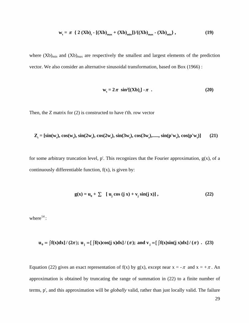
wt = { 2 (Xb)t - [(Xb)max + (Xb)min]}/{(Xb)max - (Xb)min} , (19)

where (Xb)min and (Xb)max are respectively the smallest and largest elements of the prediction

vector. We also consider an alternative sinusoidal transformation, based on Box (1966) :

wt = 2 sin2[(Xb)t] - . (20)

Then, the Z matrix for (2) is constructed to have t'th. row vector

Zt = [sin(wt), cos(wt), sin(2wt), cos(2wt), sin(3wt), cos(3wt),....., sin(p'wt), cos(p'wt)] (21)

for some arbitrary truncation level, p'. This recognizes that the Fourier approximation, g(x), of a

continuously differentiable function, f(x), is given by:

g(x) = u0 + [ uj cos (j x) + vj sin(j x)] , (22)

where14 :

u f(x)dx] / (2 ; u f(x)cos(j x)dx] / ( ); and v f(x)sin(j x)dx] / ( )j j0 ) . (23)

Equation (22) gives an exact representation of f(x) by g(x), except near x = - and x = + . An

approximation is obtained by truncating the range of summation in (22) to a finite number of

terms, p', and this approximation will be globally valid, rather than just locally valid. The failure

30

of the representation at the exact end-points of the [- , + ] interval can generate an

approximation error which is often referred to as "Gibb's Phenomenon". Accordingly, some

authors modify transformations such as (19) or (20) to achieve a range which is just inside this

interval. We have experimented with this refinement to the above transformations and have

found that it makes negligible difference in the case we have considered. The results reported in

section VI below do not incorporate this refinement.

In our case, the uj's and vj's in (23) correspond to elements of in (14), and so they are

estimated as part of the testing procedure15. Note that Z is random here, but only through b. Our

FRESET test involves constructing Z in this way and then testing if = 0 in (14). Under this

null, the FRESET test statistic is still central F, with 2p' and (T-k-2p') degrees of freedom. Its

non-null distribution will depend upon the form of the model mis-specification, the nature of the

regressors, and the choice of p'. This distribution will differ from that of the RESET test statistic

based on a (truncated) Taylor series of Xb. In the following discussion we use the titles

FRESETL and FRESETS to refer to the FRESET tests based on the linear transformation (19)

and the sinusoidal transformation (20) respectively.

V. A MONTE CARLO EXPERIMENT

We have undertaken a Monte Carlo experiment to compare the properties of the new FRESET

tests with those of the conventional RESET test, for some different types of model mis-

specification. Table 1 shows the different formulations of the tests that we have considered in all

parts of the experiment. Effectively, we have considered choices16 of p = 1, 2 or 3 and p' = 2 or

31

3. In the case of the RESET test, the variables whose significance is tested (i.e., the "extra" Z

variables which are added to the basic model) comprise powers of the prediction vector from the

original model under test, as in (15). For the FRESET test they comprise sines and cosines of

multiples of this vector, as in (21), once the linear transformation (19) or the sinusoidal

transformation (20) has been used for the FRESETL and FRESETS variants respectively.

Three models form the basis of our experiment, and these are summarized in Table 2. In each

case we show a particular data-generating process (DGP), or "true" model specification, together

with the model that is actually fitted to the data. The latter "null" model is the one whose

specification is being tested. Our Model 1 allows for mis-specification through static variable

omission, and corresponds to Models 6-8 (depending on the value of ) of Thursby and Schmidt

(1977, p. 638). Our Model 2 allows for a static mis-specification of the functional form, and our

Model 3 involves the omission of a dynamic effect. In each case, x2, x3, and x4 are as in Ramsey

and Gilbert (1972) and Thursby and Schmidt (1977) 17, and samples sizes of T = 20 and T = 50

have been considered.

Various values of were considered in the range [-8.0, +8.0] in the case of Models 1 and 2,

though in the latter case the graphs and tables reported below relate to a "narrower" range as the

results "stabilize" quite quickly. Values of in the (stationary) range [-0.9, +0.9] were

considered in the case of Model 3. If = 0 the fitted (null) model is correctly specified. Other

values of generate varying degrees of model mis-specification, and we are interested in the

probability that each test rejects the null model (by rejecting the null hypothesis that = 0 in

(14)), when 0. By way of convenience, we will term these rejection rates "powers" in the

32

ensuing discussion. However, care should be taken over their interpretation in the present

context. Strictly, of course, the power of the RESET or FRESET test is the rejection probability

when 0. As noted in Section II, this power can be determined (in principle), as the test

statistics are typically doubly non-central F when 0. Only in the very special case where

Z in (14) exactly coincides with the specification error, , would "powers" of the sort that we

are computing and reporting actually correspond to the formal powers of the tests. (In the case of

our Model 1, for example, this would require that the RESET test be applied by using just x2,

fortuitously, as the only "augmenting" variable, rather than augmenting the model with powers

of the prediction vector.) Accordingly, it is not surprising that, in general, the shapes of the

various graphs that are reported in the next section do not accord with that for the true power

curve for an F-test.

The error term, t , was generated to be standard Normal, though of course the tests are scale-

invariant and so the results below are invariant to the value of the true error variance. The tests

were conducted at both the 5% and 10% significance levels. As the RESET and FRESET test

statistics are exactly F-distributed if = 0, there is no "size distortion" if the appropriate F

critical values are used - the nominal and true significance levels coincide. Precise critical values

were generated using the Davies (1980) algorithm as coded in the "DISTRIB" command in the

SHAZAM (1993) package. Each component of the experiment is based on 5,000 replications.

Accordingly, from the properties of a binomial proportion, the standard error associated with a

rejection probability, (in the tables 3-5), takes the value 1 50001

2 , which takes its

33

maximum value of 0.0071 when = 0.5. The simulations were undertaken using SHAZAM

code on both a P.C. and a DEC Alpha 3000/400.

VI. MONTE CARLO RESULTS

In this section, we present the results of Monte Carlo experiments designed to gather evidence on

the power of the various RESET and the above FRESET tests in Table 1 for each of the three

models listed in Table 2. The experimental results and the graphs of the rejection rates are given

below. For convenience we will refer to the graphs below as “power” curves. As discussed

above, it is important to note that these are not conventional power curves. Only results for case

3 for the RESET and case 2 for the FRESET tests in Table 1 are presented in detail for reasons

which will become evident below. The entries in tables 2-5 are the proportions of rejections of

the null hypothesis. Not surprisingly, for all models considered, the RESET, FRESETL and

FRESETS tests exhibit higher rejection rates at the 10% significance level than at the 5% level.

However, the “pattern” of the “power” curves is insensitive to the choice of significance level,

hence we will focus on the 10% significance level in the remainder of the discussion.

Generally, the patterns of the “power” curves differ only marginally when the sample size is

increased from 20 to 50. The results for a sample size of 50 display higher power than the

comparable sample size 20 results, reflecting the consistency of the tests. This is also in accord

with the fact that, the larger sample size yields “smoother” power curves in the FRESETL and

FRESETS cases for Models 1 and 2.

34

The probability of rejecting a true null hypothesis when specification error is present depends, in

part, on the number of variables included in Zt. In general, our results indicate, regardless of the

type of mis-specification, that the use of p = 3 in the construction of Zt as in (15) yields the most

powerful RESET test. However, this does not always hold true such as in the case of Model 3

where the RESET test with only the term yt2 included in the auxiliary regression yields higher

“power” for relatively large positive mis-specification ( 0.3) and large negative mis-

specification ( -0.7).

The FRESETL and FRESETS tests with p = 3 terms are generally the most powerful of these

tests. The pattern of the “power” curves tends to fluctuate less and the results indicate higher

rejection rates than in the comparable p = 2 case. This is not surprising, as we would expect a

better degree of approximation to the omitted effect as more terms are included. However, the

ability to increase the number of test variables included in the auxiliary regression is constrained

by the degrees of freedom. In the remainder of this paper, we will focus primarily on the RESET

test with p = 3 and the FRESET tests with p = 3.

In all cases, the FRESET tests perform equally as well as, and in many cases yield higher

“powers” than, the comparable RESET tests. A comparison of the rejection rates of the various

tests for the three models considered indicates FRESETL is the most powerful test for Models 1

and 2. The FRESETS test yields higher “power” for Model 3 than the FRESETL and RESET

tests, with the exception of high levels of mis-specification, where FRESETL exhibits higher

rejection rates. The FRESETS test yields higher rejection rates than the comparable RESET test

for Models 1 and 2, with two exceptions. These are, first, Model 1 in the presence of a high

35

degree of mis-specification; and, second, Model 2 in the presence of positive levels of mis-

specification ( 0). However, FRESETL yields higher rejection rates than the RESET test for

the above two exceptions. The FRESETL test dominates the RESET test for Model 3.

The “power” of the RESET test is excellent for Models 1 and 2, and p = 3, with sample size 50.

Then, for larger coefficients of the omitted variable, the proportion of rejections increases to

100.0%. For Model 1, the use of the squares, cubes and fourth powers of the predicted values as

the test variables for the RESET test results in “power” which generally increases as the

coefficient of the omitted variable becomes increasingly negative. In the presence of positive

coefficients of the omitted variable, the rejection rate generally increases initially as the level of

mis-specification increases but decreases as the coefficient of the omitted variable continues to

increase. However, “power” begins to marginally increase again at moderate levels of mis-

specification ( = 3).

Our results for Model 2 indicate the “power” of the RESET test increases as the coefficient of

the omitted variable increases for lower and higher levels of mis-specification. This result

generally holds, but as can be seen by Figure 7, it is possible for “power” to decrease as the level

of mis-specification increases. The test yields low “power” at positive levels of mis-specification

for a sample size of 20 when there is an omitted multiplicative variable. For Model 3 and both

sample sizes, the rejection rate initially increases as the coefficient of the omitted variable

increases and then falls as the degree of mis-specification continues to increase.

36

The powers of the FRESETL and FRESETS tests are excellent for Models 1 and 2, when p = 3.

The proportion of rejections increases to 100% as the coefficient of the omitted variable

increases, with the exception of the FRESETS test18 for Model 1. The inclusion of 3 sine and 3

cosine terms of the predicted values as the test variables for the FRESETL and FRESETS tests

results in “power” generally increasing as the coefficient of the omitted variable increases for

Models 1 and 2 with both sample sizes. However, as can be seen by Figure 8, it is possible for

the rejection rate to decrease as the coefficient of the omitted variable increases in the p = 2

case. For Models 1 and 2 the “power” curve increases at a faster rate and is “smoother” for

sample size 50.

For Model 3, our results indicate that the rejection rate increases initially as the coefficient of the

omitted variable increases and then decreases as the level of mis-specification continues to

increase for positive omitted coefficients of the lagged variable. However, the rejection rate

increases as mis-specification increases for negative coefficients of the omitted lagged variable.

Finally, we have also considered the inclusion of an irrelevant explanatory variable in order to

examine the robustness of the RESET and FRESET tests to an over-specification of the model.

We consider Model 1 where the DGP now becomes,

y x xt 3t 4t t 0 3 4 (24)

and the “Null” becomes,

37

y = 1.0 - 0.4x + x + t 3t 4t 2t t x + . (25)

In this case, the coefficient ( ) of the redundant regressor is freely estimated and therefore we

cannot consider a range of pre-assigned values. Our results indicate that the “power” results

differ negligibly from the true significance levels, as the rejection rates fall within two maximum

standard deviations19 of the size. That is, the tests appear to be quite robust to a simple over-

specification of the model.

VII. CONCLUSIONS

In this paper we have considered the problem of testing a regression relationship for possible mis-

specification in terms of its functional form and/or selection of regressors, in the spirit of the family

of "variable-addition" tests. We have proposed a new variant of Ramsey's (1969) RESET test,

which uses a global (rather than local) approximation to the mis-specified part of the conditional

mean of the model. Rather than basing the variable-addition procedure on a polynomial terms of

prediction vector from the basic model, we suggest the use of a Fourier series approximation. Two

ways of transforming the predicted values are considered, so that they lie in an admissible range for

such an approximation - a linear transformation gives rise to what we have termed the FRESETL

test, while a sinusoidal transformation results in what we have called the FRESETS test.

These two new test statistics share the property of the usual RESET statistic of being exactly F-

distributed under the null hypothesis of no conditional mean mis-specification, at least in the

context of a model with non-stochastic regressors and spherical disturbances. We have undertaken

38

a Monte Carlo experiment to determine the power properties of the two variants of the FRESET

test, and to compare these with the power of the RESET test for different forms of model mis-

specification, and under varying choices of the number of "augmentation" terms in all cases. Our

simulation results suggest that using the global Fourier approximation may have advantages over

using the more traditional (local) Taylor's series approximation in terms of the tests' abilities to

detect mis-specification of the model's conditional mean.

Our results also suggest that using a Fourier approximation with three sine and cosine terms results

in a test which performs well in terms of "power". The empirical rates of rejection for false model

specifications exhibited by the FRESET tests are at least as great as (and generally greater than)

those shown by the RESET test. The FRESETL test is generally the best overall when the mis-

specified model is static, while the FRESETS test is best overall when the model is mis-specified

through the omission of a dynamic effect. In practical terms, this favours a recommendation for

using the latter variant of the test.

Although the proposals and results that are presented in this paper seem to offer some

improvements on what is, arguably, the most commonly applied "variable-addition" test in

empirical econometric analysis, there is still a good deal of research to be undertaken in order to

explore the features of both the RESET and the FRESET tests in more general situations. Contrary

to earlier apparent "evidence", such as that of Thursby (1979, 1982) it is now well recognised (e.g.,

Pagan (1984, p.127), Godfrey (1988, p.107), and Porter and Kashyap (1984)) that the RESET test

is not robust to the presence of autocorrelation and/or heteroskedasticity in the model's errors. The

same is clearly true of the FRESET tests. Work in progress by the authors investigates the degree

39

of size-distortion of these tests, and their ability to reject falsely specified models, in these more

general situations. As well as considering the same forms of the RESET and FRESET tests that are

investigated in this paper, we are also exploring the properties of the corresponding tests when the

robust error covariance matrix estimators of White (1980) and Newey and West (1987) are used in

their construction. In these cases, as well as in the case of models in which the null specification is

dynamic and/or non-linear in the parameters, asymptotically valid (Chi square) counterparts to the

RESET and FRESET tests are readily constructed, as in section II.D above. The finite-sample

qualities of these variants of the tests are also under investigation by the authors.

40

REFERENCES

Amemiya, T. (1977), A Note on a Heteroscedastic Model, Journal of Econometrics, 6, 365-370.

Anderson, T. W. (1971), The Statistical Analysis of Time Series, Wiley, New York.

Anscombe, F. J. (1961), Examination of Residuals, Proceedings of the Fourth Berkeley Symposium on

Mathematical Statistics and Probability, 1, 1-36.

Bahadur (1960), Stochastic Comparison of Tests, Annals of Mathematical Statistics, 31, 276-295.

Bahadur (1967), Rates of Convergence of Estimates and Test Statistics, Annals of Mathematical Statistics, 38, 303-

324.

Basu, D. (1955), On Statistics Independent of a Complete Sufficient Statistic, Sankhya , 15, 377-380.

Bera, A. K. and C. M. Jarque (1982), Model Specification Tests: A Simultaneous Approach, Journal of

Econometrics, 20, 59-82.

Bera, A. K. and C. R. McKenzie (1987), Additivity and Separability of the Lagrange Multiplier, Likelihood Ratio

and Wald Tests, Journal of Quantitative Economics, 3, 53-63.

Box, M. J. (1966), A Comparison of Several Current Optimization Methods, and the Use of Transformations in

Constrained Problems, Computer Journal, 9, 67-77.

Breusch, T. S. (1978), Testing for Autocorrelation in Dynamic Linear Models, Australian Economic Papers, 17,

334-355.

Breusch, T. S. and A. R. Pagan (1979), A Simple Test for Heteroscedasticity and Random Coefficient Variation,

Econometrica, 47, 1287-1294.

Christensen, L. R., D. W. Jorgensen and L. J. Lau (1971), Conjugate Duality and the Transcendental Logarithmic

Production Function, (abstract), Econometrica, 39, 255-256.

Christensen, L. R., D. W. Jorgensen and L. J. Lau (1973), Transcendental Logarithmic Production Frontiers, Review

of Economics and Statistics, 55, 28-45.

David, H. A. (1981), Order Statistics, Wiley, New York.

Davidson, R. and J. G. MacKinnon (1981), Several Tests for Model Specification in the Presence of Alternative

Hypotheses, Econometrica, 49, 781-793.

41

Davidson, R. and J. G. MacKinnon (1993), Estimation and Inference in Econometrics, Oxford University Press,

Oxford.

Davies, R. B. (1980), The Distribution of a Linear Combination of 2 Random Variables: Algorithm AS 155,

Applied Statistics, 29, 323-333.

Durbin, J. (1954), Errors in Variables, Review of the International Statistical Institute, 22, 23-32.

Durbin, J. (1970), Testing for Serial Correlation in Least squares regression When Some of the Regressors Are

Lagged Dependent Variables, Econometrica, 38, 410-421.

Eastwood, A. and L. G. Godfrey (1992), The Properties and Constructive Use of Mis-specification Tests for

Multiple Regression Models, in L. G. Godfrey (ed.), The Implementation and Constructive Use of Mis-

specification Tests in Econometrics, Manchester University Press, Manchester, 109-175.

Eastwood, B.J. and A.R. Gallant (1991), Adaptive Rules for Semiparametric Estimators that Achieve Asymptotic

Normality, Econometric Theory, 7, 307-340.

Engle, R. F. (1982), Autoregressive Conditional Heteroscedasticity With Estimates of the Variance of U.K.

Inflation, Econometrica, 50, 987-1007.

Gallant, A. R. (1981), On the Bias in Functional Forms and an Essentially Unbiased Form: The Fourier Flexible

Form, Journal of Econometrics, 15, 211-245.

Garbade, K. (1977), Two Methods of Examining the Stability of Regression Coefficients, Journal of the American

Statistical Association, 72, 54-63.

Geweke, J. (1981), The Approximate Slopes of Economeric Tests, Econometrica, 49, 1427-1442.

Giles, J.A. and D.E.A. Giles (1993), Pre-Test Estimation and Testing in Econometrics: Recent Developments,

Journal of Economic Surveys, 7, 145-197.

Godfrey, L.G. (1978), Testing Against General Autoregressive and Moving Average Error Models when the

Regressors Include Lagged Dependent Variables, Econometrica, 46, 1293-1302.

Godfrey, L. G. (1988), Mis-specification Tests in Econometrics: The Lagrange Multiplier Principle and Other

Approaches, Cambridge University Press, Cambridge.

Godfrey, L. G. (1996), Mis-specification Tests and Their Uses in Econometrics, Journal of Statistical Planning and

Inference, 49, 241-260.

42

Godfrey, L. G., M. McAleer and C. R. McKenzie (1988), Variable Addition and Lagrange Multiplier Tests for

Linear and Logarithmic Regression Models, Review of Economic Studies, 70, 492-503.

Goldfeld, S. M. and R. E. Quandt (1965), Some Tests for Homoscedasticity, Journal of the American Statistical

Association, 60, 539-547.

Harrison, M. J. and B. P. M. McCabe (1979), A Test for Heteroscedasticity Based on Ordinary Least Squares

Residuals, Journal of the American Statistical Association, 74, 494-499.

Hausman, J. A. (1978), Specification Tests in Econometrics, Econometrica, 46, 1251-1272.

Hendry, D.F. (1980), Econometrics: Alchemy or Science? , Economica, 47, 387-406.

Jarque, C. J. and A. K. Bera (1980), Efficient tests for Normality, Homoscedasticity and Serial Independence of

Regression Residuals, Economics Letters, 6, 255-259.

Jarque, C. J. and A. K. Bera (1987), A Test for Normality of Observations and Regression Residuals, International

Statistical Review, 55, 163-172.

Johnston, J. (1960), Statistical Cost Analysis, McGraw-Hill, New York.

Krämer, W. and H. Sonnberger (1986), The Linear Regression Model Under Test, Physica-Verlag, Heidelberg.

Lee, J. H. H. (1991), A Lagrange Multiplier Test for GARCH Models, Economics Letters, 37, 265-271.

MacKinnon, J. G. and L. Magee (1990), Transforming the Dependent Variable in Regression Models, International

Economic Review, 31, 315-339.

McAleer, M. (1987), Specification Tests for Separate Models: A Survey, in M. L. King and D. E. A. Giles (eds.),

Specification Analysis in the Linear Model, Routledge and Kegan Paul, London, 146-196.

McAleer, M. (1995), Sherlock Holmes and the Search for Truth: A Diagnostic Tale, reprinted in L. Oxley et al.

(eds.), Surveys in Econometrics, Blackwell, Oxford, 91-138.

Magee, L. (1987), Approximating the Approximate Slopes of LR, W and LM Test Statistics, Econometric Theory,

3, 247-271.

Milliken, G. A. and F. A. Graybill (1970), Extensions of the General Linear Hypothesis Model, Journal of the

American Statistical Association, 65, 797-807.

Mitchell, K. and N. M. Onvural (1995), Fourier Flexible Cost Functions: An Exposition and Illustration Using

North Carolina S & L's, mimeo., College of Management, North Carolina State University.

43

Mitchell, K. and N. M. Onvural (1996), Economies of Scale and Scope at Large Commercial Banks: Evidence From

the Fourier Flexible Functional Form, forthcoming, Journal of Money, Credit and Banking.

Mizon, G. E. (1997a), Inferential Procedures in Nonlinear Models: An Application in a U.K. Cross Section Study of

Factor Substitution and Returns to Scale, Econometrica, 45, 1221-1242.

Mizon, G. E. (1977b), Model Selection Procedures, in M. J. Artis and A. R. Nobay (eds.), Studies in Modern

Economic Analysis, Blackwell, Oxford, 97-120.

Newey, W. and K. West (1987), A Simple, Positive-Definite, Heteroskedasticity and Autocorrelation Consistent

Covariance Matrix, Econometrica, 55, 703-708.

Ohtani, K. and J. A. Giles (1993), Testing Linear Restrictions on Coefficients in a Linear Model With Proxy

Variables and Spherically Symmetric Disturbances, Journal of Econometrics, 57, 393-406.

Pagan, A. R. (1984), Model Evaluation by Variable Addition, in D. F. Hendry and K. F. Wallis (eds.), Econometrics

and Quantitative Economics, Blackwell, Oxford, 103-133.

Pagan, A. R. and A. D. Hall (1983), Diagnostic Tests as Residual Analysis, Econometric Reviews, 2, 159-218.

Pesaran, M. H. (1974), On the Problem of Model Selection, Review of Economic Studies, 41, 153-171.

Phillips, G. D. A. and B. P. M. McCabe (1983), The Independence of Tests for Structural Change in Econometric

Models, Economics Letters, 12, 283-287.

Phillips, G. D. A. and B. P. M. McCabe (1989), A Sequential Approach to Testing for Structural Change in

Econometric Models, in W. Krämer (ed.), Econometrics of Structural Change, Physica-Verlag, Heidelberg,

87-101.

Porter, R. D. and A. K. Kashyap (1984), Autocorrelation and the Sensitivity of RESET, Economics Letters, 14, 229-

233.

Ramsey, J. B. (1969), Tests for Specification Errors in Classical Linear Least-Squares Regression Analysis, Journal

of the Royal Statistical Society, B, 31, 350-371.

Ramsey, J. B. (1983), Comment on 'Diagnostic Tests as Residual Analysis' , Econometric Reviews, 2, 241-248.

Ramsey, J. B. and R. Gilbert (1972), A Monte Carlo Study of Some Small Sample Properties of Tests for

Specification Error, Journal of the American Statistical Association, 67, 180-186.

Ramsey, J. B. and P. Schmidt (1976), Some Further Results in the Use of OLS and BLUS Residuals in Specification

Error Tests, Journal of the American Statistical Association, 71, 389-390.

44

Salkaever, D.S. (1976), The Use of Dummy Variables to Compute Prediction Errors and Confidence Intervals,

Journal of Econometrics, 4, 393-397.

Savin, N. E. (1984), Multiple Testing, in Z. Griliches and M. D. Intriligator (eds.), Handbook of Econometrics, Vol.

2, North-Holland, Amsterdam, 827-879.

Schwager, S. J. (1984), Bonferroni Sometimes Loses, American Statistician, 38, 192-197.

SHAZAM (1993), SHAZAM Econometrics Program: User's Reference manual, Version 7.0, McGraw-Hill, New

York.

Theil, H. (1965), The Analysis of Disturbances in Regression Analysis, Journal of the American Statistical

Association, 60, 1067-1079.

Theil, H. (1968), A Simplification of the BLUS Procedure for Analyzing Regression Disturbances, Journal of the

American Statistical Association, 63, 242-251.

Thursby, J. G. (1979), Alternative Specification Error Tests: A Comparative Study, Journal of the American

Statistical Association, 74, 222-223.

Thursby, J. G. (1982), Mis-specification, Heteroskedasticity, and the Chow and Goldfeld-Quandt Tests, Review of

Economics and Statistics, 64, 314-321.

Thursby, J. G. (1989), A Comparison of Several Specification Error Tests for a General Alternative, International

Economic Review, 30, 217-230.

Thursby, J. G. and P. Schmidt (1977), Some Properties of Tests for Specification Error in a Linear Regression

Model, Journal of the American Statistical Association, 72, 635-641.

White, H. (1980), A Heteroskedastic-Consistent Covariance Matrix and a Direct Test for Heteroskedasticity,

Econometrica, 48, 421-448.

White, H. (1982), Maximum Likelihood Estimation of Mis-specified Models, Econometrica, 50, 1-25.

White, H. (1987), Specification Tests in Dynamic Models, in T. Bewley (ed.), Advances in Econometrics - Fifth

World Congress, Vol. 1, Cambridge University Press, New York, 1-58.

White, H. (1994), Estimation, Inference and Specification Analysis, Cambridge University Press, Cambridge.

Wu, D. M. (1973), Alternative Tests of Independence Between Stochastic Regressors and Disturbances,

Econometrica, 41, 733-750.

45

46

FOOTNOTES

We are grateful to Karlyn Mitchell for helpful correspondence in relation to the use of

Fourier functional forms, and for supplying unpublished material; and to Lindsay Tedds

for her excellent research assistance; and to Peter Kennedy, John Small and Michael

Veall for their helpful comments. This research was supported by University of Victoria

Internal Research Grant #1-41566.

1. Lee (1991) shows the equivalence of ARCH(p) and GARCH (p,q) tests under the null,

for a constant q, where p is any natural number.

2. Its distribution under the alternative is discussed in section 3 below.

3. Essentially, this follows from Basu's (1955) Independence Theorem. For example, see

Anderson (1971, pp. 34-43, 116-134, 270-276) and the asymptotic extensions discussed

by Mizon (1977a, b).

4. For some general discussion of this point, see Phillips and McCabe (1983), Pagan and

Hall (1983), and Pagan (1984, pp. 116-117, 125-127). Phillips and McCabe (1989) also

provide extensions to other tests where the statistics can be expressed as ratios of

quadratic forms in a Normal random vector.

5. For a more comprehensive discussion of this point, see Giles and Giles (1993, pp. 176-

180).

6. A biased test is one whose power can fall below its significance level in some region of

the relevant parameter space.

7. Clearly, this plim is zero if the null is true, because then both (RSS/T) and (USS/T) are

consistent estimators of 2 .

47

8. For example, see Geweke (1981), Magee (1987), and Eastwood and Godfrey (1992,

p.132).

9. For instance, the SHAZAM (1993) package adopts this approach. Clearly, the first power

cannot be used as an extra regressor in the "augmented" equation as the design matrix

would then be perfectly collinear.

10. Note that is being approximated by Z .

11. For example, see Ramsey (1969) and Thursby and Schmidt (1977).

12. In view of the Monte Carlo evidence provided by Thursby and Schmidt (1977), in

principle it would also be interesting to consider multivariate Fourier expansions in terms

of the original regressors.

13. If the data have to be positive, as in the case of cost functions, then a positive interval

such as [c, c+2] would be appropriate.

14. The range of summation in (4.4) is from j = 1 to j = ; the ranges of integration in (4.5)

are each from - to +.

15. The parameter u0 gets "absorbed" into the coefficient of the intercept in the model (3.2).

16. We found that setting p' > 3 resulted in a singular matrix when constructing the FRESET

tests. Eastwood and Gallant (1991) suggest that setting the number of parameters equal to

the sample size raised to the two-thirds power will ensure consistency and asymptotic

normality when estimating a Fourier function. Setting p' = 2 or p' = 3 is broadly in

keeping with this for our sample sizes. As Mitchell and Onvural (1996) note, increasing

p' will increase the variance of test statistics. In the context of the FRESET test it seems

wise to limit the value of p'.

48

17. Ramsey and Gilbert (1972, p.185) provide data for two series, x1 and x2, for a sample size

of T = 10. (We follow them in "repeating" these values to generate regressors which are

"fixed in repeated samples" when considering samples of size T = 20, 50.) As in Thursby

and Schmidt (1977), x3 = x1 + x2; and x4 = x12/10.

18. For FRESETS, the number of rejections is greater than 90% for higher levels of mis-

specification.

19. As calculated by binomial proportions.

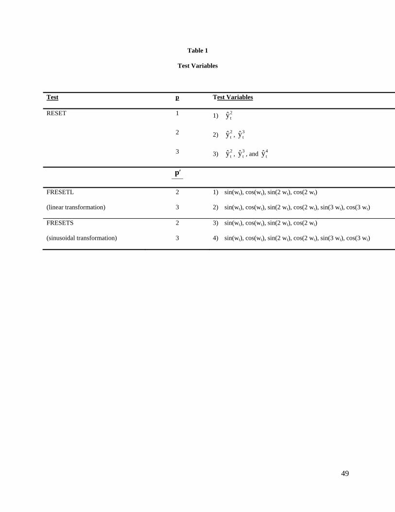
49

Table 1

Test Variables

Test p Test Variables

RESET 1 1) yt2

2 2) yt2 , yt

3

3 3) yt2 , yt

3 , and yt4

p

FRESETL 2 1) sin(wt), cos(wt), sin(2 wt), cos(2 wt)

(linear transformation) 3 2) sin(wt), cos(wt), sin(2 wt), cos(2 wt), sin(3 wt), cos(3 wt)

FRESETS 2 3) sin(wt), cos(wt), sin(2 wt), cos(2 wt)

(sinusoidal transformation) 3 4) sin(wt), cos(wt), sin(2 wt), cos(2 wt), sin(3 wt), cos(3 wt)

50

Table 2

Models

Model Specification Problem

1 DGP: y = 1.0 - 0.4x + x x +t 3t 4t 2t t

Omitted Variable

Null: y x xt 3t 4t t 0 3 4 (omitted static effect)

2 DGP: y = 1.0 - 0.4x + x 1 x +t 3t 4t 2t t

Incorrect Functional Form

Null: y x xt 3t 4t t 0 3 4 (omitted multiplicative effect)

3 DGP: y = 1.0 - 0.4x yt 3t 4t t-1 t + x + + Incorrect Functional Form

Null: y x xt 3t 4t t 0 3 4 (omitted dynamic effect)

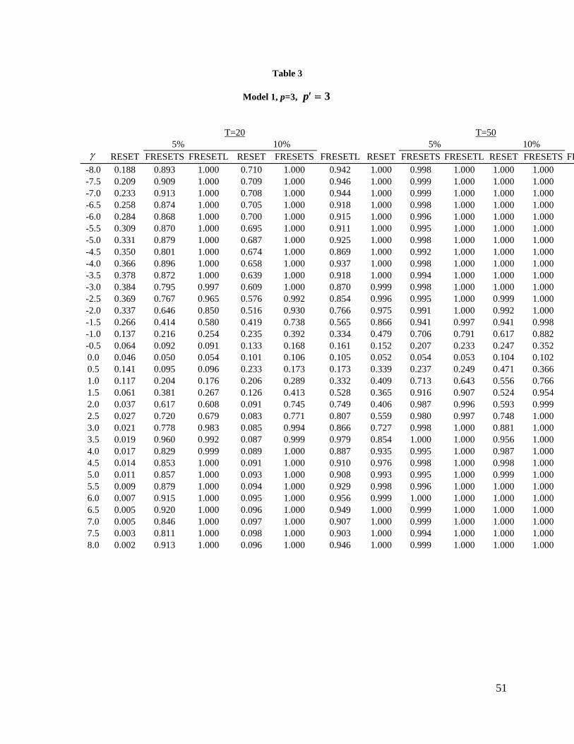
51

Table 3

Model 1, p=3, p 3

T=20 T=50

5% 10% 5% 10% RESET FRESETS FRESETL RESET FRESETS FRESETL RESET FRESETS FRESETL RESET FRESETS FR

-8.0 0.188 0.893 1.000 0.710 1.000 0.942 1.000 0.998 1.000 1.000 1.000 -7.5 0.209 0.909 1.000 0.709 1.000 0.946 1.000 0.999 1.000 1.000 1.000 -7.0 0.233 0.913 1.000 0.708 1.000 0.944 1.000 0.999 1.000 1.000 1.000 -6.5 0.258 0.874 1.000 0.705 1.000 0.918 1.000 0.998 1.000 1.000 1.000 -6.0 0.284 0.868 1.000 0.700 1.000 0.915 1.000 0.996 1.000 1.000 1.000 -5.5 0.309 0.870 1.000 0.695 1.000 0.911 1.000 0.995 1.000 1.000 1.000 -5.0 0.331 0.879 1.000 0.687 1.000 0.925 1.000 0.998 1.000 1.000 1.000 -4.5 0.350 0.801 1.000 0.674 1.000 0.869 1.000 0.992 1.000 1.000 1.000 -4.0 0.366 0.896 1.000 0.658 1.000 0.937 1.000 0.998 1.000 1.000 1.000 -3.5 0.378 0.872 1.000 0.639 1.000 0.918 1.000 0.994 1.000 1.000 1.000 -3.0 0.384 0.795 0.997 0.609 1.000 0.870 0.999 0.998 1.000 1.000 1.000 -2.5 0.369 0.767 0.965 0.576 0.992 0.854 0.996 0.995 1.000 0.999 1.000 -2.0 0.337 0.646 0.850 0.516 0.930 0.766 0.975 0.991 1.000 0.992 1.000 -1.5 0.266 0.414 0.580 0.419 0.738 0.565 0.866 0.941 0.997 0.941 0.998 -1.0 0.137 0.216 0.254 0.235 0.392 0.334 0.479 0.706 0.791 0.617 0.882 -0.5 0.064 0.092 0.091 0.133 0.168 0.161 0.152 0.207 0.233 0.247 0.352 0.0 0.046 0.050 0.054 0.101 0.106 0.105 0.052 0.054 0.053 0.104 0.102 0.5 0.141 0.095 0.096 0.233 0.173 0.173 0.339 0.237 0.249 0.471 0.366 1.0 0.117 0.204 0.176 0.206 0.289 0.332 0.409 0.713 0.643 0.556 0.766 1.5 0.061 0.381 0.267 0.126 0.413 0.528 0.365 0.916 0.907 0.524 0.954 2.0 0.037 0.617 0.608 0.091 0.745 0.749 0.406 0.987 0.996 0.593 0.999 2.5 0.027 0.720 0.679 0.083 0.771 0.807 0.559 0.980 0.997 0.748 1.000 3.0 0.021 0.778 0.983 0.085 0.994 0.866 0.727 0.998 1.000 0.881 1.000 3.5 0.019 0.960 0.992 0.087 0.999 0.979 0.854 1.000 1.000 0.956 1.000 4.0 0.017 0.829 0.999 0.089 1.000 0.887 0.935 0.995 1.000 0.987 1.000 4.5 0.014 0.853 1.000 0.091 1.000 0.910 0.976 0.998 1.000 0.998 1.000 5.0 0.011 0.857 1.000 0.093 1.000 0.908 0.993 0.995 1.000 0.999 1.000 5.5 0.009 0.879 1.000 0.094 1.000 0.929 0.998 0.996 1.000 1.000 1.000 6.0 0.007 0.915 1.000 0.095 1.000 0.956 0.999 1.000 1.000 1.000 1.000 6.5 0.005 0.920 1.000 0.096 1.000 0.949 1.000 0.999 1.000 1.000 1.000 7.0 0.005 0.846 1.000 0.097 1.000 0.907 1.000 0.999 1.000 1.000 1.000 7.5 0.003 0.811 1.000 0.098 1.000 0.903 1.000 0.994 1.000 1.000 1.000 8.0 0.002 0.913 1.000 0.096 1.000 0.946 1.000 0.999 1.000 1.000 1.000

52

Table 4

Model 2, p=3, p 3

T=20 T=50 5% 10% 5% 10%

RESET FRESETS FRESETL RESET FRESETS FRESETL RESET FRESETS FRESETL RESET FRESETS F-1.0 1.000 0.891 1.000 1.000 1.000 0.922 1.000 0.995 1.000 1.000 1.000 -0.9 1.000 0.865 1.000 1.000 1.000 0.902 1.000 0.989 1.000 1.000 1.000 -0.8 1.000 0.924 0.994 1.000 0.999 0.950 1.000 0.998 1.000 1.000 1.000 -0.7 0.996 0.910 0.832 1.000 0.954 0.937 1.000 0.994 1.000 1.000 1.000 -0.6 0.883 0.938 0.843 0.980 0.942 0.958 1.000 0.998 1.000 1.000 1.000 -0.5 0.339 0.931 0.996 0.604 0.999 0.953 1.000 0.996 1.000 1.000 1.000 -0.4 0.013 0.926 1.000 0.037 1.000 0.950 0.309 0.998 1.000 0.481 1.000 -0.3 0.243 0.866 0.999 0.391 1.000 0.909 0.870 0.989 1.000 0.926 1.000 -0.2 0.880 0.735 0.874 0.945 0.947 0.847 1.000 0.994 1.000 1.000 1.000 -0.1 0.404 0.221 0.231 0.552 0.363 0.340 0.899 0.697 0.776 0.952 0.862 0.0 0.046 0.050 0.054 0.101 0.105 0.106 0.043 0.049 0.048 0.094 0.101 0.1 0.387 0.216 0.290 0.539 0.428 0.339 0.898 0.694 0.847 0.947 0.917 0.2 0.014 0.647 0.809 0.032 0.902 0.766 0.148 0.975 1.000 0.290 1.000 0.3 0.022 0.851 0.980 0.076 0.995 0.899 0.729 0.991 1.000 0.888 1.000 0.4 0.015 0.892 0.945 0.090 0.973 0.930 0.955 0.993 1.000 0.994 1.000 0.5 0.005 0.825 0.940 0.047 0.969 0.873 0.984 0.981 1.000 0.998 1.000 0.6 0.001 0.912 1.000 0.021 1.000 0.938 0.994 0.993 1.000 1.000 1.000 0.7 0.001 0.831 1.000 0.014 1.000 0.873 0.999 0.988 1.000 1.000 1.000 0.8 0.000 0.840 1.000 0.020 1.000 0.882 1.000 0.991 1.000 1.000 1.000 0.9 0.001 0.910 1.000 0.041 1.000 0.939 1.000 0.998 1.000 1.000 1.000 1.0 0.001 0.936 1.000 0.099 1.000 0.960 1.000 0.997 1.000 1.000 1.000

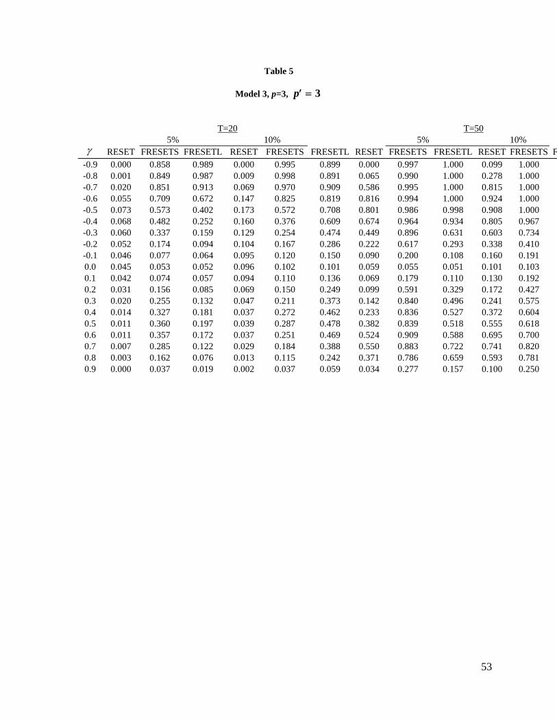
53

Table 5

Model 3, p=3, p 3

T=20 T=50 5% 10% 5% 10%

RESET FRESETS FRESETL RESET FRESETS FRESETL RESET FRESETS FRESETL RESET FRESETS F-0.9 0.000 0.858 0.989 0.000 0.995 0.899 0.000 0.997 1.000 0.099 1.000 -0.8 0.001 0.849 0.987 0.009 0.998 0.891 0.065 0.990 1.000 0.278 1.000 -0.7 0.020 0.851 0.913 0.069 0.970 0.909 0.586 0.995 1.000 0.815 1.000 -0.6 0.055 0.709 0.672 0.147 0.825 0.819 0.816 0.994 1.000 0.924 1.000 -0.5 0.073 0.573 0.402 0.173 0.572 0.708 0.801 0.986 0.998 0.908 1.000 -0.4 0.068 0.482 0.252 0.160 0.376 0.609 0.674 0.964 0.934 0.805 0.967 -0.3 0.060 0.337 0.159 0.129 0.254 0.474 0.449 0.896 0.631 0.603 0.734 -0.2 0.052 0.174 0.094 0.104 0.167 0.286 0.222 0.617 0.293 0.338 0.410 -0.1 0.046 0.077 0.064 0.095 0.120 0.150 0.090 0.200 0.108 0.160 0.191 0.0 0.045 0.053 0.052 0.096 0.102 0.101 0.059 0.055 0.051 0.101 0.103 0.1 0.042 0.074 0.057 0.094 0.110 0.136 0.069 0.179 0.110 0.130 0.192 0.2 0.031 0.156 0.085 0.069 0.150 0.249 0.099 0.591 0.329 0.172 0.427 0.3 0.020 0.255 0.132 0.047 0.211 0.373 0.142 0.840 0.496 0.241 0.575 0.4 0.014 0.327 0.181 0.037 0.272 0.462 0.233 0.836 0.527 0.372 0.604 0.5 0.011 0.360 0.197 0.039 0.287 0.478 0.382 0.839 0.518 0.555 0.618 0.6 0.011 0.357 0.172 0.037 0.251 0.469 0.524 0.909 0.588 0.695 0.700 0.7 0.007 0.285 0.122 0.029 0.184 0.388 0.550 0.883 0.722 0.741 0.820 0.8 0.003 0.162 0.076 0.013 0.115 0.242 0.371 0.786 0.659 0.593 0.781 0.9 0.000 0.037 0.019 0.002 0.037 0.059 0.034 0.277 0.157 0.100 0.250