Diagnosing Sources of U.S. Seasonal Forecast Skill

X. Quan, M. Hoerling, J. Whitaker, G. Bates, and T. Xu

(NOAA-CIRES Climate Diagnostics Center, Boulder, Colorado)

Submitted to Journal of Climate

Revised 26 September 2005

*Corresponding author: quan.xiaowei@noaa.gov

Climate Diagnostics Center

NOAA, R/CDC1

325 Broadway

Boulder, CO 80305-3328

Phone: 303-497-6807

Fax: 303-497-6449

1

Abstract

In this study we diagnose the sources for the contiguous U.S. seasonal forecast skill that are

related to sea-surface temperature (SST) variations using a combination of dynamical and

empirical methods. The dynamical methods include ensemble simulations with 4 atmospheric

general circulation models (AGCM) forced by observed monthly global SSTs from 1950 to

1999, and ensemble AGCM experiments forced by idealized SST anomalies. The empirical

methods involve a suite of reductions of the AGCM simulations. These include uni- and multi-

variate regression models that encapsulate the simultaneous and 1-season lag linear connections

between seasonal mean tropical SST anomalies and U.S. precipitation and surface air

temperature.

Nearly all of the AGCM skill in U.S. precipitation and surface air temperature, arising from

global SST influences, can be explained by a single degree of freedom in the tropical SST field

--- that associated with the linear atmospheric signal of El Niño/Southern Oscillation (ENSO).

The results support previous findings regarding the preeminence of ENSO as a U.S. skill source.

Our diagnostic methods exposed another skill source that appeared to be of non-ENSO origins.

In late fall, when the AGCM simulation skill of U.S. temperatures peaked in absolute value and

in spatial coverage, the majority of that originated from SST variability in the sub-tropical west

Pacific Ocean and the South China Sea. Hindcast experiments were performed for 1950-1999

that revealed most of the simulation skill of U.S. seasonal climate to be recoverable at 1-season

lag.

2

The skill attributable to the AGCMs was shown to achieve parity with that attributable to

empirical models derived purely from observational data. The diagnostics promote the

interpretation that only limited advances in U.S. seasonal prediction skill should be expected

from methods seeking to capitalize on sea surface predictors alone, and that advances which may

occur in future decades could be readily masked by inherent multi-decadal fluctuations in skill of

coupled ocean-atmosphere systems.

1. Introduction

Foremost among U.S. seasonal forecast skill sources are the state of tropical sea surface

temperatures (SST), a relation stemming from the sensitivity of atmospheric stationary waves

and storm tracks to tropical forcing (e.g., Hoskins and Karoly, 1981; Held et al. 1989). To date,

the El Niño-Southern Oscillation (ENSO), that is typified by east tropical Pacific SST variations,

is the single phenomena of the ocean-atmosphere system demonstrated to render U.S. seasonal

forecasts skillful (e.g., Barnett and Prisendorfer 1987; Barnston 1994; Higgins et al. 2004). That

skill is elevated in the winter and spring seasons, at which time it also exhibits a large spatial

footprint over the U.S. due to the planetary-scale of ENSO-forced circulation variations.

The question we pose is whether ENSO constitutes the sole tropical SST source of U.S. seasonal

forecast skill. To be sure, empirical and simulation studies have identified sensitivities to SST

forcings outside the east tropical Pacific. For example, the influence of SST anomalies over a

region north of the equator in the tropical west Pacific was highlighed by Palmer and Owen

3

(1986) as contributing to the severe U.S. winter of 1976-77. Empirical support for such a

connection was provided by studies of the relation between atmospheric circulation patterns and

proxies for tropical convection (Livezey and Mo 1987). The influence of SST anomalies over

the warm pool regions of the Indian and western Pacific Oceans have also been shown to play

roles in the U.S. climate, such as during 1997 and 1998 (Pegion et al. 2000), and during 1998-

2002 when the U.S. experienced protracted warm and dry conditions (Kumar et al. 2001,

Hoerling and Kumar 2003). Idealized modeling experiments, both linear dynamical models

forced by tropical heating (e.g., Ting and Yu 1998; Chen and Newman 1998), and perpetual-

mode general circulation models forced with idealized SSTs (Geisler at al. 1985; Barsugli and

Sardeshmukh 2002), have confirmed robust Pacific-North American responses to forcings

located outside the classic ENSO region of the east tropical Pacific.

Historical simulations of 20th Century climate using atmospheric general circulation models

(AGCMs) subjected to observed monthly evolving global SSTs are now permitting diagnosis of

sensitivity patterns under realistic conditions. The availability of multi-AGCMs, each run

numerous times over an historical period, permits a more robust and reliable identification of

atmospheric response patterns associated with tropical forcing than hitherto possible. Using a

46-member ensemble of 50-year experiments spanning 1950-1999 from 4 different AGCMs,

Hoerling and Kumar (2002) subjected the monthly 500 hPa height fields of the multi-model

ensemble to a empirical orthogonal function (EOF) analysis. These yielded evidence for at least

4 different characteristic atmospheric patterns associated with tropical SST variability. The

leading one was the well-known ENSO teleconnection. However, the additional patterns

accounted for up to 50% of the local boundary forced variance over parts of North America, and

4

appeared to be of non-ENSO tropical origin. It is unknown whether these additional sensitivities

contribute to skill of U.S. surface temperature and precipitation predictions.

An ensemble of AGCM runs yields a wealth of information about the sensitivity of the

atmosphere to observed SST anomalies. However, it is often not clear what the relationship

between the prescribed SST and the GCM ensemble mean atmospheric response is. For

example, further diagnosis is necessary to determine how many degrees of freedom in the SST

field are actually involved in producing the simulated atmospheric signals. This is useful

information, since it defines the relevant phase space of SST patterns that need to be predicted

accurately for a seasonal forecast. Even if information can be obtained about the SST patterns

from the AMIP runs (see e.g. Hoerling and Kumar, 2002), one is still left wondering how

predictable those patterns are. Goddard and Mason (2002) have examined the predictability

issue by running a complementary ensemble of GCM runs, but instead of the traditional AMIP

approach, they use SSTs that are persisted (as a simple prediction) for one season. In this way

they were able to investigate the predictability of the seasonal mean atmospheric state based on

forecast SSTs rather than simultaneous SSTs. Here we attempt to address both the question of

how many degrees of freedom are needed to reproduce the ensemble mean GCM response over

the U.S., and the question of how predictable that response is, using an empirical statistical

model trained on the 46 member multi-model GCM ensemble.

Our study combines AGCM and empirical methods to diagnose the simulation and hindcast skill

of seasonal surface climate over the U.S. during 1950-1999. The data sets and methods are

5

presented in section 2. Section 3 presents results in which the seasonally varying skill of surface

temperature and precipitation are described and diagnosed. In addition to the expected ENSO

contribution, a non-ENSO source of skill is discovered. Section 4 focuses on a diagnosis of this

additional source of U.S. skill. A summary and concluding comments are given in section 5.

2. Data and Method

a. Observations

Monthly observed U.S. surface temperature and rainfall data for 1950-1999 are available on a

2.5 ° grid based on the Global Historical Climate Network. Monthly sea surface temperature

analyses for 1950-1999 come from the United Kingdom Meteorological Office (UKMO) Hadley

Centre’s Global Sea-Ice and SST (HadiSST) dataset (Rayner et al. 2003). The global SSTs are

created using various techniques including reduced space optimal interpolation, and are available

on a 1° grid.

b. Atmospheric climate simulations forced by global SSTs

The sea surface temperature role in climate variability is assessed using atmospheric GCMs

forced with the specified, observed monthly variations in SSTs for 1950-1999. Multiple

integrations are begun from different atmospheric initial conditions, but in which each ensemble

member is subjected to identically specified sea surface conditions.

Four different AGCMs are used, consisting of a total of 46 simulations spaning the last half of

the 20th Century. The models used are identical to those in Hoerling and Kumar (2002). Table 1

summarizes their spatial resolutions, and the reader is refered to the indicated references for

6

details on different dynamical cores and physical parameterizations used in each model. The

atmospheric GCMs include 12 simulations using NCAR's Community Climate Model (CCM3;

Kiehl et al. 1998), 12 using NCEP's Medium Range Forecast model (MRF9; Kumar et al. 1996),

10 with the European Centre-Hamburg Model (ECHAM3; Roeckner et al. 1992) and 12

simulations using the climate model of the Geophysical Fluids Dynamics Laboratory (GFDL;

Broccoli and Manabe 1992).

Our analysis of the AGCMs is based on the combined 46-member ensemble. The ensemble

mean seasonal anomaly for each of the four models is calculated relative to the respective

models’ climatology for each of the 600 overlaping seasons during 1950-1999. The ensemble

mean anomaly of each model is standardized by its SST-boundary forced (external) variance, as

described in more detail in Hoerling and Kumar (2002). The ensemble mean seasonal anomaly

for each of the 4 GCMs is calculated, with anomalies computed relative to the respective model's

1950-99 climatology. Because these models possess different sensitivities to identical boundary

forcing, we standardized the ensemble anomaly of each GCM by its own external variance, also

calculated for the 1950-99 period. These are then averaged across the 4 models to yield a grand,

standardized anomaly (consisting implicitly of the average anomaly for 46 discrete realizations).

Actual anomalies are recovered by multiplying the standardized anomaly of each season by the

4-model averaged external variance. These standardized anomalies are then averaged across the

four models in order to produce the multi-model, standardized anomaly. Actual anomalies are

recovered by multiplying the standardized anomaly of each season by the four model averaged

external variance. Horizonal and vertical resolutions of these models are listed in Table 1. In an

analysis examining the impact of different ensemble mean methods, Byun (2002, personal

7

communication) compared the skill of this 46-member ensemble mean and the skill of another

ensemble mean of the same 46-member but using a weighted average in which the weights were

different for each member and determined by minimizing the difference between the model

ensemble mean and the verification field. Byun’s results indicated that for the 1950-99 50-year

period the simulation skill of the weighted ensemble mean is virtually the same as the skill of

the ensemble mean used in this study.

c. Atmospheric climate simulations forced by idealized SSTs

Simulations using a fixed idealized SST anomaly over the subtropical western Pacific are

conducted, the pattern of which is discussed in section 4. This anomaly is specified and fixed

throughout the seasonal cycle, and is added to the seasonally varying climatological SSTs. A

total of 20 14-month simulations, beginning from randomly selected 1 November atmospheric

initial conditions, were performed with NCAR’s CCM3, one of the models included in our multi-

model suite forced by realistic SSTs.

d. Empirical climate prediction model

The empirical model is based on uni- and multi-variate linear regression that relates a set of

seasonally averaged fields of tropical (20°S-20°N) SST (the predictors) to a set of seasonally

averaged model simulated fields of U.S. surface temperature and precipitation (the predictands)

(see Fig. 1). Regression models are developed both for the simultaneous and 1-season lag

relationships between predictor-predictand pairs. This allows us to estimate the relevant SST

subspace both for the zero-lag (contemporaneous) GCM simulation, and the 1-season lag GCM

prediction. Unlike the Goddard and Mason study, we do not rerun the GCM with predicted

8

SSTs, but instead use the lag-covariance relationships between the SST and the simulated

atmospheric response from the AMIP integrations to estimate what the GCM prediction would

be, given actual predicted SSTs. This approach assumes that the relationship between SSTs and

the atmospheric response over the U.S. is linear. This hypothesis is tested in the next section by

verifying that the empirical model can reproduce the GCM simulation skill over the U.S.. The

empirical statistical model we use is very similar to others used for seasonal prediction (e.g.,

Barnston 1994), except for the fact that in our case the model is trained on the 46-member

ensemble average of multi-model simulations described in section 2b, instead of observed

atmospheric states. By training on the model ensemble mean, our tool describes the relation

between atmospheric signal and tropical SST forcing, whereas similar tools trained on the brief,

“single realization” of observed states neccesarily predict a blend of signal and noise given a

tropical SST state.

In the construction of the statistical model, the raw, seasonal predictor and predictand data are

first pre-filtered using EOFs in a manner outlined by Barnett and Preisendorfer (1987) and as

implemented by Barnston (1994). We retain N-EOFs in predictor and M-EOFs in predictand

fields, where the truncation is determined by applying the formalism of North et al. (1982). For

the tropical SSTs, N is chosen to be 5 for all 12 overalapping seasons. For U.S. precipitation, M

is chosen to be 6 for all seasons, while M is chosen to be 9 for U.S. surface temperature. The

North et al. (1982) analysis suggested that the EOF modes higher than a critical order are

statistically indistinguishable. Therefore, we do not include higher order SST modes in our

analysis and treat the higher order SST modes as noise. The EOF expansion coefficients

(principal components) are then normalized by the square root of their eigenvalues, and the EOF

9

basis is calculated independently for each of 12-overlapping 3-month seasons. The cross-

covariance matrix is calculated in EOF space, and the predicted EOF expansion coefficients are

transformed back to a 2.5 degree latitude/longitude grid. A parallel set of uni-variate regression

models is constructed to isolate the contribution of ENSO to the predictands of interest. The uni-

variate regression uses only the 1st EOF (i.e. ENSO) mode of the tropical SST as a predictor, and

6 (9) EOF modes of the U.S. precipitation (surface temperature) as predictands. The uni-variate

regression is also trained on the multi-model ensemble mean.

d. Verification methodology

We employ a deterministic measure of skill based upon the temporal correlation. Monthly mean

surface air temperature and precipitation anomalies are obtained by subtracting the 30-year

climatology of 1970-99 for each calender month from the monthly mean values at each grid

point over our domain (see Fig. 2). Three-month mean anomalies are then calculated from the

monthly mean anomalies. The same method is applied to the output from the 46-member AGCM

simulations. Verification is performed using the three-month mean anomalies.

All the uni- and multi-variate empirical model simulations and hindcasts for each 3-month

season employ a cross-validation procedure in which the model is constructed from the co-

variance matrix of 49-years of seasonal data, excluding the target season for the simulation or

hindcast. In this manner, a “new” empirical model is constructed for each year, and also for each

season. The 1951-1999 skill of the empirical model simulations and hindcasts was then

calculated in the way identical to that applied to the AGCM simulations. When calculating

spatial averages of correlation skill for U.S. surface temperature, coastal gridpoints (indicated by

“o” in Figure 2) are excluded because local temperature skill at those areas can be largely

10

detemined by the prescribed SST in AGCM simulations.

The field significance of the correlation skill maps for each variable and for each of the twelve

3-month seasons is tested in a manner similar to Livezey and Chen (1983). For a given variable

and season, Monte Carlo experiments of 3000 samples are first performed by randomly ordering

the 50-year time sequence of observed fields and then calculating temporal correlations with the

true 1950-99 observed time sequence. From these, we compute the probability distribution of

the number of U.S. points in Fig. 2 having temporal correlations exceeding 90% local

significance (r > 0.25). Then, the number of U.S. grid points (N0) at 95% of the accumulated

obtained distribution constitutes the minimum number necessary for passing field significance.

In order that a correlation skill pattern be field significant, the actual number of locally

significant grid-points (N) must exceed N0, i.e. the ratio N/N0 must exceed 1.

3. Diagnosing SST skill sources

a. U. S. Precipitation

The annual cycle of simulation skill, and its sources, averaged over the U.S. is summarized in

Fig. 3. Correlation skill of the AGCM simulations is low in all seasons (top), having a minor

maximum during winter (thick solid line). Its primary source is tropical SSTs, as demonstrated

by the ability of the multivariate regression model simulation skill (thin solid line) to fully

recover that of the global SST forced AGCMs. Further, a single pattern of the tropical SST

variations is able to explain this skill (dotted curve), namely the ENSO signature of the tropical

east Pacific (not shown). The simulation skills are field significant in winter and spring, but not

so in summer and early fall (bottom).

11

Inspection of the spatial patterns of skill reveals the univariate regression model to be superior to

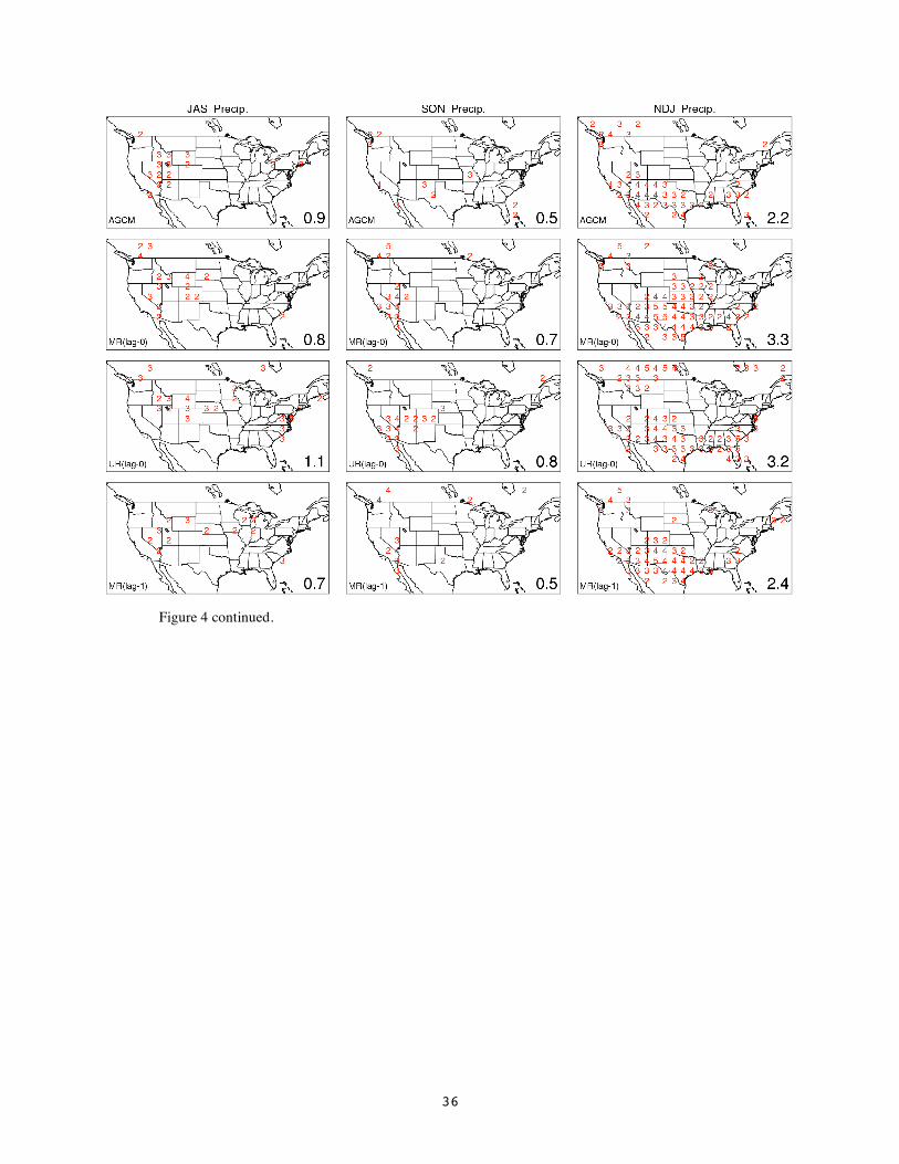
the AGCM simulation in select regions. Figure 4 shows the temporal anomaly correlation for the

U.S. domain, and the plotted values are the truncated correlation skill scores (x 10) at all points

exceeding 90% significance. The lower right corner of each panel plots the ratio N/N0, which

denotes field significance for values >1. The six columns correspond to partially overlapping 3-

month seasons, and the top three panels of each column display the AGCM simulation skill, the

multivariate regression model skill, and the univariate regression model skill, respectively.

During January-February-March (JFM), significant skill covers nearly half the domain in the

univariate model, and mimics the spatial footprint of ENSO’s influence on U.S. precipitation

(e.g. Ropelewski and Halpert 1989, Kiladis and Diaz 1989). This pattern is only weakly

discernable in the AGCM simulation skill. Throughout all remaining seasons, it is found that the

AGCM simulation skill is generally surpassed by a reduced-space representation of the relation

between SST and model U.S. precipitation.

The lower panels of each column display the zero-lead hindcast skill using the multivariate

model. These recover virtually all of the 50-yr averaged AGCM simulation skill. The uni-variate

model often performs better than the multi-variate model. This is so because ENSO SSTs are the

primary skill source, and the fact that such an ENSO pattern can itself be skillfully predicted at

short lead times.

b. U. S. Surface Temperature

The SST source for U.S. surface temperature skill is found to be detemined not by ENSO alone,

in contrast to the pure ENSO-source that was diagnosed for U.S. precipitation skill. Figure 5

12

summarizes the area-averaged skill of the three simulation data sets, from which it is evident that

the three simulation skills are comparable during winter and spring, but that the AGCM skill is

greater than either multi- or univariate regressions in summer and fall. Note that the AGCM

skill is field significant in all seasons (bottom), contrary to the empirical model skill which are

not field signifcant from September-November (SON) through November-January (NDJ).

There is a distinct NDJ seasonal peak in simulation skill, at which time the U.S. averaged 50-yr

mean skill exceeds 0.36. The field significance exceeding 99.9% is all the more remarkable

when compared to the lack of field significance by either empirical model simulation. By

contrast, the coincidence in skill of the three simulations during winter and spring indicates that

ENSO’s linear signal is the primary source. An ENSO SST source appears to impart little skill

during other seasons as indicated by the large divergence between the AGCM and regression

model skills at those times. These other SST sources could be of tropical origin, but are

unaccounted for by our truncated multivariate model, or they could be of extratropical sea

surface origin. It is also possible that non-linear processses associated with the atmospheric

response to SST forcing are important contributors to the AGCM skill, relations also not

represented in the regression models.

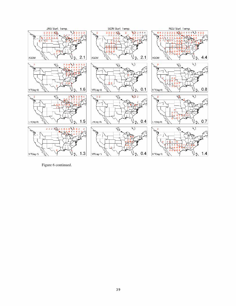
The spatial distribution of surface temperature skill, shown in Fig. 6, offers further insights on

SST sources. There is little appreciable difference in skill patterns occurring among the three

simulations during winter and spring --- the similarity with the univariate model skill confirms

once again that the linear component of the ENSO-forced atmospheric signal is of primary

consequence. On the other hand, the AGCM simulation skill is greater in both its coverage and

13

its absolute value than either regression model during summer and fall. The footprint differs

from the linear ENSO contribution which, as illustrated by the univariate skill map, is confined

to the southern U.S..

Shown in the lower panels of Fig. 6 are the hindcast skills for the multivariate model. These

recover much of the simulation skill of U.S. surface temperature during winter/spring, consistent

with the fact that the linear ENSO influence is of greatest relevance and that such SSTs are

themselves skillfully predicted at zero-lead. In contrast, they fail to reproduce the extensive

spatial coverage of the AGCM’s simulation skill during the NDJ season.

4. A Subtropical West Pacific Skill Source

We first explore the SST structure associated with the AGCM’s high skill over the northern U.S.

during November-December-January. The green box in Fig. 7 keys on the region of high

AGCM skill, and is the domain over which surface air temperatures are averaged in order to

generate a 1950-1999 time series. The correlation of that time series with SSTs across the global

oceans is shown by the shaded contours, and the analysis is performed using both the AGCM

(top) and observed (bottom) surface air temperatures. Maximum correlations exceeding +0.5

occur with SSTs over the northwest Pacific Ocean and the South China Sea, and there is also

some suggestion of an ENSO relation in so far as +0.3 correlations occur with over the tropical

east Pacific. However, the fact that an ENSO-region correlation is very weak in the observations

suggests it is unlikely an appreciable skill source. By contrast, the consistencey between the

simulated and observed high correlations over the Western Pacific suggests that SST variations

there could be an important skill source for northern U.S. surface air temperature.

14

The coherency of their interannual fluctuations lends some support for a causal relation between

subtropical west Pacific SSTs and the northern U.S. index region’s temperatures. Figure 8

overlays the times series of the surface air temperature index and an index of SST averaged over

the west Pacific box of Fig. 7. The former is calculated from both AGCM (Fig. 8, top) and

observed (Fig. 8, bottom) surface air temperatures. For both, the correlation with the west

Pacific SST index exceeds +0.5, with warm sea surface conditions accompanying warm northern

U.S. surface temperatures. In addition to the tendency for interannual swings of each index to be

alligned, a post-1970 warming trend in both ocean and land time series also contributes to the

positive temporal correlations.

Shown in Fig. 9 is the temporal variation of our west Pacific SST index with SST elsewhere.

The coherency of an SST signature that encompasses the South China Sea, Philippine Sea, and

the subtropical west Pacific is evident. There is only a weak simultaneous relation with SSTs

over the ENSO region, again suggesting that this west Pacific source of U.S. simulation skill in

the AGCM is not an obvious proxy for ENSO’s effect.

Independent evidence for a causal link between variatons in west Pacific SSTs and U.S. surface

temperatures is provided by the additional AGCM experiments forced exclusively with SSTs

over that region. The idealized anomalous SST forcing is obtained from a composite of the SST

pattern contrasting warm and cold events (when anomalous values exceeded one standard

15

deviation) in the northern U.S. temperature (Fig.8 top), and has similar structure as outlined by

the irregular contour in Fig. 9, and encompasses the spatial domain of temporally coherent west

Pacific SST variations. A 20-member ensemble of CCM3 simulations was conducted using both

positive and negative polarities of the SST anomalies, with maximum amplitudes of 1° C. The

NDJ surface temperature anomalies of the (warm-cold) experiments is shown in the lower panel

of Fig. 10. Widespread warming covers North America, with a maximum signal over the

northern U.S. and southern Canada. This response pattern is remarkably similar with the 1950-

1999 correlation between an index of the west Pacific SSTs and both multi-model AGCM (Fig.

10, top) and observed (Fig. 10, middle) surface temperatures. Indicated hereby is that the

statistical correlation does indeed describe a a cause-effect relationship.

The implications of the above analyses is that a bivariate regression model, having west Pacific

and tropical east Pacific SST predictors, should be able to recover the AGCM simulation skill

during the NDJ season. The simulation skill of such a bivariate model is shown in Fig. 11

(middle panel). For comparison, the simulation skill of only a univariate model using the west

Pacific SST as predictor is shown in the top panel of Fig. 11. Nearly all of the AGCM’s

simulation skill over the northern U.S. during NDJ (see Fig. 6) is accounted for by a west Pacific

influence. The results of the bivariate model, which also includes the ENSO influence, almost

completely recovers the AGCM simulation skill. These calculations support the argument that

the high AGCM simulation skill for NDJ surface temperature over the northern US is attributed

to the ocean-atmosphere interactions in the Western Pacific Ocean.

16

As a final analysis, we re-examine the hindcast skill of NDJ surface temperatures, but now using

a 1-season lag bivariate regression model. The results are shown in the lower panel of Fig. 11,

and it is apparent that the vast majority of simulation skill is retained in the prediction mode.

This suggests that the west Pacific SST predictor is itself predictable and slowly evolving on the

seasonal time scale. The new subtropical SST source bears some resemblance to the 3rd CCA

SST mode in Barnston and Smith (1996). However, our analysis revealed that the SST variation

in the subtropical Northwest Pacific Ocean is not a direct response to ENSO. In fact, the SST

variation in the subtropical NW Pacific Ocean leads an out-of-phase ENSO episode by about one

year (not shown).

5. Summary and discussion

a. Summary

The sea surface temperature origins for seasonal forecast skill of U.S. precipitation and surface

air temperature have been diagnosed. The principal tool consisted of ensemble atmospheric

GCM simulations that were subjected to the known monthly varying global SSTs from 1950-

1999. The simulation skill of the resulting multi-model 46-member ensemble was evaluated,

and then diagnosed using two empirical reductions of the full AGCM data. The first consisted of

a multivariate linear regression model relating the simultaneous states of five leading tropical

SST patterns to the AGCM’s U.S. seasonal climate. The second was a univariate linear

regression model whose predictor consisted of the single leading tropical SST pattern only ---

ENSO.

Our diagnosis revealed that the AGCM simulation skill could be explained by-and-large from the

17

linear influence of tropical sea surface temperature variations. Furthermore, one degree of

freedom in those tropical SSTs, namely ENSO, was the virtually exclusive interannual skill

source originating from tropical oceans. In the case of U.S. seasonal precipitation, the univariate

regression model that encapsulated the linear ENSO signal produced simulation skill that

exceeded the AGCM simulation skill, though field significance was confined to the period late

Fall–late Spring. One interpretation for the superior precipitation skill of the univariate model is

that whereas sensitivity patterns to non-ENSO SSTs existed in the AGCMs, these were

seemingly erroneous and served to obscure the true skill source related to ENSO.

A new SST skill source, of apparent non-ENSO origins, was discovered for U.S. surface air

temperature. Although the AGCM’s winter-spring skill source was again accounted for by a

univariate linear influence of ENSO, the AGCM skill significantly exceeded that of either the

linear models during the period from late summer through Fall. During these latter seasons,

both the AGCMs’ U.S. averaged correlation skill and the spatial extent of its significant local

correlations greatly exceeded those occuring in the reduced phase space linear model simulations

based on tropical SSTs alone. Our investigation focused on the November-January season of

maximum difference in skills, and a coherent source related to SST variability over the sub-

tropical west Pacific Ocean and the South China Sea was found.

That this empircal relation constituted a cause-effect link was confirmed through analysis of an

additional suite of AGCM experiments that used an idealization of SST forcing confined to the

far west Pacific/South China Sea region. Those runs yielded a pattern of U.S., surface warming

in response to warm SST forcing that reproduced the characteristic correlation patterns derived

18

from both the globally forced multi-model ensemble and the observational data sets. A linear

bivariate regression model using only indicies of Nino3.4 and west Pacific/South China Sea

SSTs explained virtually all of the AGCM simulation skill during the NDJ season.

Hindcast experiments for 1951-1999 were generated in order to determine what elements of

skillfully simulated U.S. responses to known SST forcing could be predicted. These employed

the multivariate regression model using the 1-season lag relationships between tropical SST

predictors and the AGCM’s U.S. seasonal climate. These are analogous to zero-lead predictions,

and estimate what the AGCM predictions would have been given a forecast for the tropical

SSTs. Virtually all of the simulation skill was recovered in the hindcast experiments for the

seasons and the variables for which ENSO was the dominate source of simulation skill. The

hindcasts failed to recover the AGCM simulation skill of U.S. surface air temperature during late

summer-fall. It was demonstrated, however, that a 1-season lagged bivariate model could

recover the AGCM’s high simulation skill during fall. One conclusion drawn from the hindcasts

is that the principal SST sources of U.S. predictability can themselves be skillfully forecast at

zero-lead.

b. Discussion

Dynamical methods for U.S. climate prediction are now achieving parity with empirical

approaches (e.g., Peng et al. 2000). The key question is whether such equivalence of capability

testifies to the limitations in skill of seasonal climate prediction, as suggested by Anderson et al.

(1999), or whether it speaks to the infancy of dynamical models. Our diagnosis of the skill

sources offers the following insight on such questions.

19

The fact that the linear response to ENSO SST variability accounts for much of the AGCM skill

over the U.S. ---- particularly in winter/spring for both precipitation and temperature---- implies

that a simple regression model trained from observations should have comparable skill to the

dynamical model given sufficient data. We confirm this to be the case in Fig. 12 where the bar

graphs compare the hindcast skill of our prior multivariate model to an identical model in which

the U.S. predictand data are derived from observations. Their 50-year hindcast skills are

indistinguishable, and the reason is because both are originating from the ENSO influence whose

response is realistically modeled in the AGCMs. If there are other tropical SST skill sources in

nature, then they are evidently too small (or they occur too infrequently) to be detected and have

material effects on the 50-year averaged skill (This does not discount the possible skillful

contribution of such additional tropical sources in individual years). The preeminence of ENSO

as a U.S. skill source is further verified by the result of our singular value decomposition (SVD)

analysis. We found that the singular value of the leading SVD mode is much larger than other

SVD modes. Our result is consistent with that predicted by DelSole and Chang (2003). Our study

did identify an additional non-ENSO skill contributor, but as was the case with ENSO, a linear

empirical model could be used to capitalize upon that source too.

In this study, our analysis has been foucused on the multi-model ensemble mean. Treating

predictions from different models as a single ensemble increases the ensemble size and reduces

sampling biases. Furthermore the skill of the ensemble mean is found to be higher than the skill

of individual AGCMs included (figure not shown). In operational practice, the skill of seasonal

forecasts may be further raised by applying more sophisticated multi-model combination

20

strateges (e.g. Goddard et al. 2003, Barnston et al. 2004). The sources of skill identified in our

analysis are limited only to those that can be captured by the multi-model ensemble mean.

Additional sources may be identified when optimal ensemble average methods are applied to

maximize the skill. It is also possible that the seasonal forecast skill can be further improved, and

additional non-ENSO skill sources identified, when newer generation models are available.

The possibility that extratropical SST variations contribute to skill cannot be discounted based

upon our analysis. It is possible that the near equivalance in simulation skill between the

AGCMs and the statistical models using only tropical SST predictors (e.g., in all seasons for U.S.

precipitation, and in winter/spring for U.S. surface air temperature) is symptomatic of AGCM

biases, including the two-tier design of experiments, rather than a lack of predictive impact of

non-tropical SSTs. A important thrust for future investigation is asessing how, if at all, this

current diagnosis of U.S. seasonal forecast skill related to sea surface temperature influences is

modified when using the next generation of atmospheric GCMs. Likewise, a comparative

analysis of the AGCM skill against that of coupled ocean-atmosphere models is needed to

specifically address whether the predictability estimates, such as presented herein and in

previous studies using two-tiered systems, are applicable to fully coupled Earth System models.

Regarding the skill attributes of such fully coupled models, it should also be noted that

initialization of observed land surface conditions may be sources for U.S. skill, in addition to

ocean surface conditions. While the AGCM studied herein do employ coupled soil moisture

models of various complexity, none of the runs used observed soil moisture conditions.

21

A further open question in seasonal climate predictability concerns the expected value for skill

itself. Is an analysis of skill drawn from 50 years of data a reliable estimate of the true expected

value? To what degree does such a 50-year analysis speak to the system’s predictability in

general, and what are error bars on those estimates owing to sampling alone? Little is known

about the manner in which skill can vary over extended time periods. In so far as ENSO has been

affirmed to be the primary source of skill, it is reasonable to suspect that periods of low ENSO

variance would lead to lower U.S. climate predictability. At the same time, ENSO itself accounts

for only a small fraction of U.S. climate variability (e.g., Hoerling and Kumar 2002), and thus

purely atmospheric intrinsic variations could also impact skill fluctuations. As a further

diagnosis of the statistical robustness of our skill, we have used 650 years of output from an

integration of an unforced coupled ocean-atmosphere model (NCAR’s CCSM2; Kiehl and Gent

2004). This model posseses ENSO related variability that is sufficiently realistic for our

purposes in so far as the model’s ENSO signal over the U.S. explains roughly the same fraction

of interannual variance as does the observed ENSO signal (not shown). Another empirical

multivariate model was developed for 1-season lag relationships between tropical SSTs and U.S.

surface air temperature based on the first 150 years of the coupled model run. Hindcasts were

then made for the subsequent 500 years of model data. Figure 13 shows the probability densities

of independent 50-year samples of hindcast skill of U.S. surface temperature for the seasons JFM

through MAM. The 50-yr mean variations range from a low correlation skill of 0.1 and a high

value of 0.3, with a median value near 0.2. These variations arise purely due to intrinsic coupled

model noise. This result suggests that dynamical models are still needed to fully harvest the skill

source of seasonal froecasts even if the skill of dynamical models comes from just one degree of

22

freedom in the SST, since the skills of empirical methods trained on 50-year of data may have

large decadal swings.

In conclusion, it is apparent that a sound appraisal of the future prospects for U.S. seasonal

forecast skill must be founded upon an understanding of the sources for skill itself. Here we

have explored the ocean’s role, and identified a single degree of freedom in SST variations as

providing the bulk of U.S. seasonal skill. An outlook for future capabilities must also seek to

understand the sources for multi-decadal variations in skill, which our analysis indicates could

occur simply due to low frequency variations in ENSO and other intrinsic fluctuations of the

coupled ocean-atmosphere system. If multi-decadal variations in seasonal forecast skill are

sufficiently large, then they could mask technological advances in seasonal prediction

methodologies.

Acknowledgement: The authors would like to thank Dr. Arun Kumar for discussions and

suggestions during the forming of this paper. Thanks are also due to two anonymous reviewers and their critical reviews. Their comments and suggestions have improved the content of this

paper. This study is supported by funds from the NOAA OGP’s CLIVAR Program.

23

References Anderson, J. H. van den Dool, A. Barnston, W. Chen, W. Stern, and J. Ploshay, 1999: Present-

day capabilities of numerical and statistical models for atmospheric extratropical seasonal

simulation and prediction. Bull. Amer. Meteor. Soc., 80, 1349-1361

Barnett, T.P. and R.W. Preisendorfer, 1987: Origins and levels of monthly and seasonal forecast

skill for North American surface temperature determined by canonical correlation analysis. Mon.

Wea. Rev., 115, 1825-1850

Barnston, A.G., 1994: Linear statistical short-term climate predictive skill in the northern

hemisphere. J. Climate, 7, 1513-1564

Barnston, A. G. and T.M. Smith, 1996: Specification and prediction of global surface

temperature and precipitation from global SST using CCA. J. Climate, 9, 2660-2697

Barnston, A.G., S.J. Mason, L. Goddard, D.G. Dewitt, and S.E. Zebiak, 2003: Multimodel

ensembling in seasonal climate forecasting at IRI. Bull. Amer. Meteor. Soc., 84, 1783-1796

Barsugli, J.J. and P.D. Sardeshmukh. 2002: Global atmospheric sensitivity to tropical SST

anomalies throughout the Indo-Pacific basin. J. Climate, 15, 3427–3442.

Broccoli, A.J. and S. Manabe. 1992: The effects of orography on midlatitude northern hemisphere

dry climates. J. Climate, 5,1181–1201.

24

Chen, P., and M. Newman, 1998: Rossby wave propagation and the rapid development of upper-

level anomalous anticyclones during the 1988 U.S. drought. J. Climate, 11, 2491-2504.

Delsole, T. and P. Chang, 2003: Predictable component analysis, canonical correlation analysis,

and autoregressive models. J. Atmos. Sci., 60, 409-416

Geisler, J.E., M.L. Blackmon, G.T. Bates, and S . Muñoz, 1985: Sensitivity of January climate

response to the magnitude and position of equatorial Pacific sea surface temperature anomalies.

J. Atmos. Sci., 42, 1037-1049

Goddard, L. and S.J. Mason, 2002: Sensitivity of seasonal climate forecasts to persisted SST

anomalies. Clim. Dyn., 19, 619-631

Goddard, L., A.G. Barnston, and S.J. Mason, 2003: Evaluation of the IRI’s “net assessment”

seasonal climate forecasts 1997-2001. Bull. Amer. Meteor. Soc., 84, 1761-1780

Held, I. M., S. W. Lyons, and S. Nigam, 1989: Transients and the extratropical response to El

Niño. J. Atmos. Sci., 46, 163-174.

Higgins, R.W., H.-K. Kim and D. Unger. 2004: Long-lead seasonal temperature and

precipitation prediction using tropical Pacific SST consolidation forecasts. J. Climate, 17, 3398–

3414.

25

Hoerling, M. P., and A. Kumar, 2002: Atmospheric response patterns associated with tropical

forcing. J. Climate, 15, 2184-2203.

Hoerling, M. P., and A. Kumar, 2003: The perfect ocean for drought. Science, 299, 691-694.

Hoskins, B.J. and D.J. Karoly, 1981: The steady linear response of a spherical atmosphere to

thermal and orographic forcing. J. Atmos. Sci., 38, 1179-1196

Kiehl, J.T., J. J. Hack, G. B. Bonan, B. A. Boville, D. L. Williamson and P. J. Rasch. 1998: The

National Center for Atmospheric Research community climate model: CCM3. J. Climate, 11,

1131–1149.

Kiehl, J. T., and P. R. Gent , 2004: The community climate system model, version 2. J. Climate, 17,

3666–3682

Kiladis, G.N. and H.F. Diaz, 1989: Global climatic anomalies associated with extremes in the

southern oscillation. J. Climate, 2, 1069-1090

Kumar A., M. Hoerling, M. Ji, A. Leetmaa and P. Sardeshmukh. 1996: Assessing a GCM's

Suitability for Making Seasonal Predictions. J. Climate, 9, 115–129.

Kumar, A., W. Wang, M.P. Hoerling, A. Leetma, and M. Ji, 2001: The sustained North

American warming of 1997 and 1998. J. Climate, 14, 345-353

Livezey, R.E. and W.Y. Chen, 1983: Statistical field significance and its determination by Monte

26

Carlo techniques. Mon. Wea. Rev., 111, 46-59

Livezey, R.E. and K.C. Mo, 1987: Tropical-extratropical teleconnections during the Northern

Hemisphere winter: Part II: Relationships between the monthl mean Northern hemisphere

circulation patterns and proxies for tropical convection. Mon. Wea. Rev., 115, 3115-3132.

North, G.R., T.L. Bell, R.F. Cahalan, and F.J. Moeng, 1982: Sampling errors in the estimation

of empirical orthogonal functions. Mon. Wea. Rev., 110, 699-706

Palmer, T.N. and J.A. Owen. 1986: A possible relationship between some “severe” winters in

North America and enhanced convective activity over the tropical west Pacific. Mon. Wea. Rev., 114,

648–651.

Pegion, P., S. Schubert, and M. J. Suarez, 2000: An Assessment of the Predictability of Northern

Winter Seasonal Means with the NSIPP1 AGCM. NASA Tech. Memo-2000-104606, Vol. 18,

100pp.

Peng, P., A. Kumer, A.G. Barnston, L. Goddard, 2000: Simulation skills of the SST-forced

global climate variability of the NCEP-MRF9 and the Scrippts-MPI ECHAM3 models. J.

Climate, 13, 3657-3679

Rayner, N. A., D. E. Parker, E. B. Horton, C. K. Folland, L. V. Alexander, D. P. Rowell, E. C.

Kent, and A. Kaplan, 2003: Global analyses of sea surface temperature, sea ice, and night marine

air temperature since the late nineteenth century. J. Geophys. Res., 108, 4407,

27

doi:10.1029/2002JD002670

Roeckner, E., and coauthors. 1992. Simulation of the present-day climate with the ECHAM

model: Impact of model physics and resolution. Max-Plank-Institute für Meteorologie, Report

93, 171 pp. (Available from MPI für Meteorologie, Bundesstr. 55, D-20146 Hamburg,

Germany.)

Ropelewski, C. F. and M.S. Halpert, 1989: Precipitation patterns associated with the high index

phase of the southern oscillation. J. Climate, 2, 268-284

Ting, M. F. and L. H. Yu, 1998: Steady response to tropical heating in wavy linear and nonlinear

baroclinic models. J. Atmos. Sci., 55, 3565-3582.

28

Figure Captions:

Figure 1 Schemetic of the empirical model used to simulate and forecast U.S. seasonal

precipitation (P) and surface air temperature (Ts). The indicies i and j denote the seasons

used in each simulation and hindcast experiment. In the simulations, j equals to i for each

experiment. In the 1-season-lead hindcasts j is one season lag to i (e.g., when i points to

OND of 1998, j is JFM of 1999). See text for further details.

Figure 2 Grids included in the verification for precipitation (all "o" and "+" grid-points),surface

temperature (only the "+" grid-points).

Figure 3 Saptial average of the 1951-99 temporal correlation for the US precipitation (top)

and field significance values (bottom). Points above the shade are statistically significant at

95% confidence level.

Figure 4 Temporal correlation between observed and simulated/hindcast 3-month mean

anomalies of precipitation. Red numbers are the first digit of of the correlation coefficient

value at each grid-point. Having higher than 90% local significance. Black numbers shown

at bottom right corner in each panel indicate field significance level (N/N0) of the

corresponding correlation patterns. Ratios exceeding 1 indicates field significant at 95%

confidence level. Note: the “lag-0” in figure caption represents “simulation”, and “lag-1” is

used for “zero-lead hindcast” in text.

29

Figure 5 Same as Fig. 3 except for the US surface temperature.

Figure 6 Same as Fig. 4 except for the US surface temperature.

Figure 7 Spatial distribution of the correlation coefficient between SST and an index of regional

mean surface temperature over the northern U.S. (42N- 52N,120W-70W) based on AGCM

simulated (top panel) and observed (bottom panel) NDJ surface temperatures. Contour interval

0.1. Green box denotes index region for constructing land temeprature time series, and white

box index region for constructing SST time series.

Figure 8 Time series of NDJ anomalies of Northern U.S. surface temperature (black line) based

on AGCM simulations (top) and observations (bottom). Red line denotes the time series of NDJ

SSTs averaged over the Western Pacific region. Inserted boxes of Fig. 7 show the averaging

domains for contructing each time series.

Figure 9 The 1950-1999 temporal correlation between the NDJ SST anomalies and the NDJ

index of subtropical west Pacific SSTs. Contour interval 0.1. See Fig. 7 for the averaging

domain for constructing the index. The irregular white contour encloses a region of SST

variations coherent with the index region, and is used as the forcing region for idealized AGCM

simulations.

Figure 10 Spatial distribution of the correlation between the NDJ SST anomalies in the

western Pacific Ocean and the multi-AGCM ensemble mean (top panel) and observed

30

(middle panel) surface temperature anomalies. Contour interval is 0.1. The CCM3 response

to the idealized SST anomalies in the Western Pacific Ocean is shown in the bottom panel.

Contour interval is 1. C.

Figure 11 Same as Fig.6 but for the NDJ simulation skill based on a univariate regression

model using only an index of subtropical west Pacific (WP) SSTs as predictor, a bivariate

regression model using the WP and Nino 3.4 indicies as predictors (middle panel); and the

hindcast skill based on a lagged bivariate model relating ASO Nino3.4 and WP SST

anomalies to NDJ surface temperature (bottom panel),

Figure 12. The U.S. spatially averaged multivariate model hindcast skill for 1951-99 for

observed U.S. precipitation, and surface temperature using identical empirical models except that

the predicand data are derived from the AGCMs (MR(G)) in one case and from the observations

in the other case (MR(O)).

Figure 13. Probability distribution of the 50-year U.S. surface temperature skill obtained from

the 500-year simulation of the NCAR coupled climate system model

.

31

Table 1. Characteristics of the atmospheric GCMs used in the study.

SPECTRAL

RESOLUTION SIGMA

LAYERS ENSEMBLE

SIZE REFERENCE

CCM3 T42 18 12 Kiehl et al. (1998) ECHAM3 T42 18 10 Roeckner et al.(1992) GFDL R30 18 12 Broccoli and Manabe (1992) MRF9 T40 18 12 Kumar et al. (1996)

32

Figure 1 Schemetic of the empirical model used to simulate and forecast U.S. seasonal precipitation (P) and surface air temperature (Ts). The indicies i and j denote the seasons used in each simulation and hindcast experiment. In the simulations, j equals to i for each experiment. In the 1-season-lead hindcasts j is one season lag to i (e.g., when i points to OND of 1998, j is JFM of 1999). See text for further details.

Covariance Matrix of Principal

Components

P, Ts EOF-

M

P, Ts EOF-

2

P, Ts EOF-

1

SST

EOF-1

SST

EOF-2

……

……

SST

EOF-N

History of SST variation excluding predictor

season, SST(i).

History of P, Ts variation, excluding

target season,Ts(j), P(j)

SST (i)

P, Ts (j)

33

Figure 2 Grids included in the verification for precipitation (all "o" and "+" grid-points), surface temperature (only the "+" grid-points).

34

Figure 3 Saptial average of the 1951-99 temporal correlation for the US precipitation (top)

and field significance values (bottom). Points above the shade are statistically significant at 95% confidence level.

35

Figure 4 Temporal correlation between observed and simulated/hindcast 3-month mean anomalies of precipitation. Red numbers are the first digit of of the correlation coefficient value at each grid-point. Having higher than 90% local significance. Black numbers shown at bottom right corner in each panel indicate field significance level (N/N0) of the corresponding correlation patterns. Ratios exceeding 1 indicates field significant at 95% confidence level. Note: the “lag-0” in figure caption represents “simulation”, and “lag-1” is used for “zero-lead hindcast” in text.

36

Figure 4 continued.

37

Figure 5 Same as Fig. 3 except for the US surface temperature.

38

Figure 6 Same as Fig. 4 except for the US surface temperature.

39

Figure 6 continued.

40

Figure 7 Spatial distribution of the correlation coefficient between SST and an index of regional mean surface temperature over the northern U.S. (42N- 52N,120W-70W) based on AGCM simulated (top panel) and observed (bottom panel) NDJ surface temperatures. Contour interval 0.1. Green box denotes index region for constructing land temeprature time series, and white box index region for constructing SST time series.

41

Figure 8 Time series of NDJ anomalies of Northern U.S. surface temperature (black line) based on AGCM simulations (top) and observations (bottom). Red line denotes the time series of NDJ SSTs averaged over the Western Pacific region. Inserted boxes of Fig. 7 show the averaging domains for contructing each time series.

42

Figure 9 The 1950-1999 temporal correlation between the NDJ SST anomalies and the NDJ index of subtropical west Pacific SSTs. Contour interval 0.1. See Fig. 7 for the averaging domain for constructing the index. The irregular white contour encloses a region of SST variations coherent with the index region, and is used as the forcing region for idealized AGCM simulations.

43

Figure 10 Spatial distribution of the correlation between the NDJ SST anomalies in the western Pacific Ocean and the multi-AGCM ensemble mean (top panel) and observed (middle panel) surface temperature anomalies. Contour interval is 0.1. The CCM3 response to the idealized SST anomalies in the Western Pacific Ocean is shown in the bottom panel. Contour interval is 1. C.

44

Figure 11 Same as Fig.6 but for the NDJ simulation skill based on a univariate regression model using only an index of subtropical west Pacific (WP) SSTs as predictor, a bivariate regression model using the WP and Nino 3.4 indicies as predictors (middle panel); and the hindcast skill based on a lagged bivariate model relating ASO Nino3.4 and WP SST anomalies to NDJ surface temperature (bottom panel),

45

Figure 12. The U.S. spatially averaged multivariate model hindcast skill for 1951-99 for observed U.S. precipitation, and surface temperature using identical empirical models except that the predicand data are derived from the AGCMs (MR(G)) in one case and from the observations in the other case (MR(O)).

46

Figure 13 Probability distribution of the 50-year U.S. surface temperature skill obtained from the 500-year simulation of the NCAR coupled climate system model.