DI; FILE LORA

" TECHNICAL REPORT -" AD

NATICK/TR-88/021

• , CONTROL SYSTEMS FOR PLATFORMLANDINGS CUSHIONED

. (!Q) BY AIR BAGS0)

BY| EDWARD W. ROSS

JULY 1987

FINAL REPORTJULY 1985 TO AUGUST 1985I

C.

DTIO:. . ELECTIE" ' JUN 2 0 1M8

APPROVED FOR PUBLIC RELEASE; t 01988 DDISTRIBUTION UNLIMITED E

UNITED STATES ARMY NATICKRESEARCH, DEVELOPMENT AND ENGINEERING CENTER

NATICK, MASSACHUSETTS 01760-5000

AERO-MECHANICAL ENGINEERING DIR qOIgTE2. -Cto

. . . . . . . . . . . . .

The findingts contained in thin report are. Pot -to

be construed as an offiial IDepartet -of. the Army

position u lessBD des ignated. by other au~hrie

documents.

Citation of trade tames in ttiig ieport, 46esUbt

constitute airofca eU o.~rVIp

the use I ;A ~

Se u i y, , S-' . - t L-

For C lsife DoufintI

Deotloy. &y, th poe.4D~ Ahat" $~~~~conent r r 1CoTv-t" nVt

U I'LAS S I F1 FSECOR'TY CLASSIrCATICN O THIS PACE%.w F orApproved

REPORT DOCUMENTATION PAGE FOrm Approved,._TiE Date Jun30 1986la REPOR- SECURITY CLASSIFICATION lb RESTRICTIVE MARKINGS

T-ni I ass i f ied

"a SECURITY CLASSFiCATION AUTHORITY 3 DISTRIBUTION /AVAILABILITY OF REPORTApproved for public release,

2b DECLASSIFICATION / DOWNGRADING SCHEDULEidi St ri but ion unlimited

4 PERFORMING ORGANIZATION REPORT NUMBER(S) 5 MONITORING ORGANIZATION REPORT NUMBER(S)

NATICK/TR-88/02 1

6a NAME OF PERFORMING ORGANIZATION 6b OFFICE SYMBOL 7a NAME OF MONITORING ORGANIZATION(If applicable)

.. Arvv Natck RD&E Center STRNC-UE

6< ADDRESS (City, State, and ZIPCode) 7b ADDRESS(Crty, State, a w-' ZIP Code)

Kan ss St.. Natick, MA 0176C-5017

Ba NAME OF FUNDING; SPONSORING r8b OFFICE SYMBOL 9 PROCUREMENT INSTRUMENT IDENTIFICATION NUMBERORGANIZATION (If applicable)

8c ADDRESS (City, State, and ZIP Code) 10 SOURCE OF FUNDING NUMBERSPROGRAM I PROJECT TASK |WORK UNITELEMENT NO NO NO ACCESSION NO

6101 IL~i ~ 07 137

I! TITLE (Include Security Classification)

"." "rc Systemcs for Plattorm Landings Cushioned by Air Bags

12 PERSONAL AUTHOR(S)

Ecward .". Ross13a TYPE OF REPORT 13b TIME COVERED T14 DATE OF REPORT (Year, Month, Day) 15 PAGE COUNTFinal tFROM July 85 TO 5 Q8 July 43

"-. 16 SUPPLFMENTARY NOTATION

7 COSATI CODES 18. SUBJECT TERMS (Continue on reverse if necessary I _idhidnri __ ffr )FiE .p GROUP SUB-GROUP .IR DROP OPERATIONS CUSHIONING LA1NDNFW MIAUT,

AIRBAGS LANDTING AIDS- IPACT SHOCK.LATFORM LANDINGS AERIAL DELIVERY 6ONTROL SYSTEMS.

19 ABSTRACT (Continue on reverse if necessary and identify by block number)>Th s report presents an exploratory mathematical study of control systems for airdrop

ciattorr landings cushioned by airbags. The basic theory of airbags is reviewed andsc.iutions to special cases are noted. A computer program is presented, which calculates

'. hetime-dependence of the principal variables during a landing under the action of variouscontrol systems. Tw u existing control systems of open-loop type are compared with a,orceptuai feedback (closed-loop) system for a fairly typical set of landing conditions..In feedback controller is shown to have performance much superior to the other systems.

T-. feedbacks s'sterr, undergoes an interesting oscillation not present in the other systems,• scu.rce of which is investigated. Recommendations for future work are included.

* 20 DSTRIBuTION /AVAI.ABILITY OF ABSTRACT 21 ABSTRACT SECURITY CLASSIFICATION

" JNCLASSIFIED/UNLIMITED 0 SAME AS RPT 2l DTiC USERS Unclassified

'2a NAME OF RESPONSIBLE ir) V D.A. 22b TELEPHONE (Include Area Code) 22c OFFICE SYMBOL

Edward . Ross 617-651-4915 -2

DO FORM 1473, 84 MAR 83 APR edition may be, J " pn'ti ' cvhj,;" SECURITY CLASSIFICATION OF THIS PAGEAll other editions are obsolete UNCLASS I FI ED

Us .& e ~ ~ '~.'

0

PREFACE

This work is intended to explore the possibility that the performance of

airbags in cushioning the landings of airdrop platforms can be improved by

introducing automatic control of the vent opening. The work was done in the

period May to August, 1985, under Program Element 61101A, Project No. IL161101

A91A, Task No. 07, and Work Unit Accession No. 137.

Accession For

.4NTTS CGRA&I-DT)7IC TABUn'nnounced

;, ~Ju t if ica t o EDn_ _ _ _

.- " .. Distribution/

Availabllity Codes

....iand/or-

.o

IN

.- " , ,

-I,

0

.1~

0J.

U-

S

S

TABLE OF CONTENTS

Page

Abstract ii

Preface iii

List of Figures vi

List of Tables vii

1. Introduction 1

2. Basic Airbag Equations 2

3. Solutions for Special Cases 6

4. Control Systems 8

5. Numerical Analysis of Landings with Controls 10

S6. Discussion 18

7. Conclusions and Recommendations 22

8p . References 24

Appendix A - Computer Programs 25

* Appendix B - Perturbation Analysis 39

Appendix C - List of Symbols 32

VA

.gv

a,

"p

S

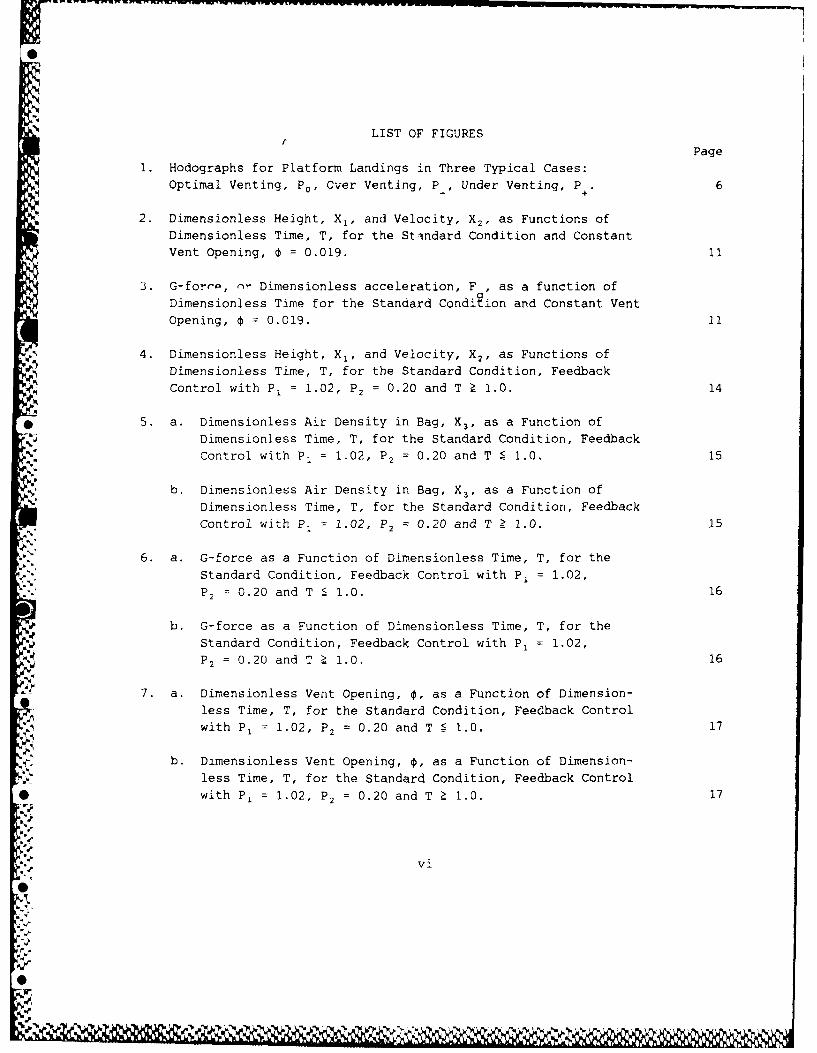
LIST OF FIGURES

Page1. Hodographs for Platform Landings in Three Typical Cases:

Optimal Venting, P0 , Over Venting, P , Under Venting, P . 6- +

2. Dimensionless Height, X1, and Velocity, X2, as Functions ofDimensionless Time, T, for the Standard Condition and ConstantVent Opening, = 0.019. 11

3. G-forrp, nr Dimensionless acceleration, F , as a function ofDimensionless Time for the Standard Condition and Constant VentOpening, 0 = 0.019. 11

4. Dimensionless Height, X1 , and Velocity, X2, as Functions ofDimensionless Time, T, for the Standard Condition, FeedbackControl with P1

= 1.02, P2 = 0.20 and T Z 1.0. 14

q

5. a. Dimensionless Air Density in Bag, X3, as a Function of

Dimensionless Time, T, for the Standard Condition, FeedbackControl with P1 = 1.02, P2 = 0.20 and T : 1.0. 15

b. Dimensionless Air Density in Bag, X3, as a Function ofDimensionless Time, T, for the Standard Condition, FeedbackControl with P1

= 1.02, P2 = 0.20 and T Z 1.0. 15

• 6. a. G-force as a Function of Dimensionless Time, T, for theStandard Condition, Feedback Control with P1 = 1.02,P2

= 0.20 and T = < 1.0. 16

b. G-force as a Function of Dimensionless Time, T, for theStandard Condition, Feedback Control with P, = 1.02,P2

= 0.20 and T 1.0. 16

7. a. Dimensionless Vent Opening, 0, as a Function of Dimension-less Time, T, for the Standard Condition, Feedback Control

with P1 = 1.02, P2 = 0.20 and T 5 1.0. 17

b. Dimensionless Vent Opening, $, as a Function of Dimension-

less Time, T, for the Standard Condition, Feedback Control* with P1 1.02, P2 = 0.20 and T 1.0. 17

Sv

• vi

LIST OF TABLES

Table Page

1 Typical Values for Physical Constants 4

2 Typical Dimensionless Parameter Values 4

3 Optimal Results for Blow-off Patch 13

4 Computed Results for Feedback Control Law 13

5 Oscillation Extremes for Feedback Control Law 19

0

"',.

-a

;-S

,..vi_

S, ,=

.. , .h*Bo.

- -- - .-.-. ~ , u.., -. - . .. .n-wr, .... mn. ~w,.wrrb~- - - - -- W flr r. - -------

0

1. iN R(DUCTION

In recent years the Army has devoted considerable attention to the use of

pneumatic devices (airbags) in reducing the landing shock of various

* air-delivery systems. A number of different designs have been investigated

experimentally by Nykvist', Patterson 2 and others. The fundamental theory was

* preserted first by Browning3, then extended by Esgar and Morgan'.

The present report describes a preliminary study of possible systems for

automatic control in the course of a platform landing cushioned by a simple,

cylindrical airbag. The original impetus for the study was a discussion

* between Dr. C.K. Lee and the author, in which Dr. Lee mentioned that small

motors are now available that have response times in the millisecond range.The possibility of using such a motor to drive a device for opening and

-3 closing the vent of an airbag led to the investigation reported here.

The basic theory of airbags is reviewed in the next section and put into a

*dimensionless form slightly different from (but wholly equivalent to) that of

v Browning3. The resulting nonlinear system of three ordinary differential

equations cannot in general be integrated exactly. However, Section 3

describes two solutions in closed form that can be obtained under certain

assumptions about the vent area. Several other plausible control systems are

discussed in Section 4, and Section 5 presents the results of numerical

* solutions, comparing the performances of these control systems. The results

are discussed and conclusions presented in Sections 6 and 7.

.5-

0Z

2. BASIC AIRBAG EQUATIONS

This section is closely related to the analyses given by Browning3 and

Esgar and Morgan". The context and basic assumptions are described below.

a. The load, W, is descending steadily beneath a parachute and is

attached to the top of a plane platform, dropping vertically and oriented

horizontally, during the entire impact process. The initial velocity of

descent is Vo.

b. An airbag in the form of a cylinder with a vertical axis and

horizontal end surfaces is attached to the underside of the platform. The

airbag has height H and cross-sectional area AB and initially contains air at

atmospheric pressure, Pa. There is a vent to the atmosphere with area Av .

c. At time t = 0 the lower face of the bag makes contact with the ground.

Thereafter, the bag preserves always the same cross-section area, AB, but the

volume decreases as the platform descends.

d. The pressure, p, and mass-density p, of the air in the bag are related

by the ideal gas law,

P/Pa = ( Pa ()

where pa is the density of air at atmospheric pressure and y is the ratio of

the specific heats, specifically y = 1.4 for air.

With these assumptions the equations of motion can be written as a system

of three nonlinear ordinary differential equations in

y = height of platform above ground

V = velocity (positive upward)

p = mass density of air in bag

namely

dy/dt = V (2)

dV/dt = g [-1 4 (D RB)/W] (3)Am Ad(py)/dt = CvAv~aq (4)

-2-

where

g acceleration of gravity

D = canopy drag

RB = force transmitted to platform from airbag

q = speed of air flow from vent

Cv = vent flow coefficient

further

D = i A V2 C (5)2 a c D

Ac = drag area of canopy (6)

CD = drag coefficient of canopy (7)

RB = (P-Pa)AB (7)

q =2 JoV 2 + S (8)

Equation (8) is Bernoulli's law for the flow of air out the vent or

* orifice. Jo is a constant that affects the definition of the flow upstream of

the vent in Bernouili's law, and S has a form which depends on the pressure in

the bag. Let

PC = critical pressure Pall + (y-l)/2 ] /(Y- I ) - 1.893 pa (9)

Then

S = [2y/(y-l)) [(p/p) - (Pa/Pa) ] if p < Pc (10)

if P ' Pc (11)

Equation (2) is merely the definition of velocity, conservation of

platform momentum is embodied in Equation (3), and Equation (4) expresses

conservation of air-mass in the bag. Collectively they are, when combined

with Equations (1) and (5) to (11), a system of three nonlinear, ordinary

* differential equations for the three functions y, V and p. The initial

conditions are

at t = 0, y = H, V = -V 0 and p = a'

* The equations can be put in dimensionless form by defining

* . J = y/H, X2 = V/V, X3 = P/Pa' t = TH/Vo

=LI : PaAb/W, 2 = gH/V0 2, 0.3 2 7Pa/[(Y-)PaV 2

S= pc/pa

O : OaAcV 2CD/(2W), a6 : Jo

.0 P/pa Q q/Vo Av/AB,

%-3-

0

W

which leads to the system of equations

dxi,/dT = X2 (12)

dX2/dT = a2Fg (13)

dX3/dT = -(X2X3 + QC v)/x1 (14)

wherei~r = X3 Y, OL4 : 14(-)/1-1 (15),(16)

Fg = -1 + a5X22 + 7l(n-l) (17)

Q = [c6xz2 + a30] (18)

a = (n/x3)-1 l OL. (19)

i = (Y-l)((l/X4 - r/)) Z Ct 4 (20)

and the initial conditions are

xi = 1, x2 = -1, x3 = 1 at T =0 (21)

Typical values for the physical constants in the analysis are listed in

0. Table 1 and the corresponding dimensionless parameters aj (J = 1....6) are

given in Table 2.

TABLE 1

Typical Values for Physical Constants

H initial height of platform 3 ft

% V0 initial velocity of platform 30 ft/s% AB cross sectional area of bag 10 ft2

W weight of platform and load 1000 lbs

"p air pressure 2117 lb/ft 2

P a mass density of air .002 lb s 2/ft4

ag acceleration of gravity 32.2 ft/s

* A drag area of canopy 1000 ft2

A " cross-sectional area of vent I ft2

v

',

TABLE 2

Typical Dimensionless Parameter Values

- a1 = 21.17" a 2 = .1073

CL 8233

-O 4. a .893

L a5 '9C

90

-4-0

1* ~ % ~ave,

0

if the airbag has any effect, we may assume that

tnroughout most of the motion because CD < 1, 04 < ai, and it is plausible to

neglect the term in (17) that contains cis, although some inaccuracy can result

near T = 0. A similar argument causes us to neglect the term in (18) that

involves Oe, although the accuracy may be questionable near T = 0, especially

since the value of Jo is not well-specified beyond saying that Jo = 0(l).

The remainder of this paper will be based on the equations (12) to (16),

the modified equations (17) and (18),

Fg -1 + acl( - 1) (22)

Q =(ue~) 3 (23)

and (19) to (21).

0 With these approximations, the equations involve three dimensionless

parameters, a0, a2 and a3. We can see at a glance that model tests of the

platform-airbag system will encounter scaling problems unless the model tests

are carried out in a suitable, artificial atmosphere. For, if 0.2 is to be the

same for model and prototype, we must have VH the same, but a3 implies that

V must be the same for model and prototype if both are tested in the same

medium.

The energy possessed by the platform can be found by observing that the

potential energy is Wy and the kinetic energy is WV2/(2g). Then

C : (total energy)/(initial energy)

" (20L2xI + X22)/(2C2 + 1) (24)

-" The purpose of the airbag is to decelerate the platform so its vertical

,- velocity is zero when the platform strikes the ground, i.e., x1 = X2 = 0 at

same time, Tf. The airbag has, therefore, to completely dissipate the initial

*energy.

0<

k-5-S°"'

3. SOLUTIONS FOR SPECIAL CASES

In general the system of equations is nonlinear and cannot be solved

exactly in closed form. However, in certain special cases exact or

approximate solutions can be found, and it is convenient to describe these

here.

It is instructive first to think qualitatively about the behavior of the

system. For this purpose, hodograph plots of three more or less typical cases

are shown in Figure 1. All start, of course, from the initial point, xi = 1,

X2 = -1. The path Po is the trajectory followed in an ideal case where the

system reaches the point xi = x2 = 0 at time, Tf, possibly under the action of

some type of control system. A case where the bag is vented too freely, and

the platform crashes into the ground, i.e., x2 < 0 when xi = 0, exhibits a

0 trajectory like P_. Contrarily, P+ shows a path when the bag is not vented

enough, and the platform bounces off the bag, i.e., X2 0 when xi > 0.LXJN.

"II

"i' P

0

IN

• ... IT= 0

.'-- Figure 1: Hodographs for platform-landings in three typical Cases:5Optimal Venting, P., Overventing, P, Underventing, P •% N A k h N

"W"% N'i K -6

" " "w " 'e " ' .w ." ' '. " -, w"w • .,.

0

The first special case is that in which $ 0, i.e., the vent is closed.

An exact solution is obtainable in implicit form in this case,

f(xi) {1 + 2o(l+1L)(1-x1) + 2L102(-1 1 (1-xII-)}

X2 = -f2(x1) X3 = X1 1 = Xi (29)

-gT(xJ) = f f- (u)duX1

This solution resembles that of the trajectory P+ in Figure 1 if it is

followed long enough. The above solution loses validity when the function

f(xi) = 0, i.e., when X2 = 0. The values of xi and T at which this occurs

depend oniy on al, (12 and 1, not on (13.

An important special case is obtained if we demand that the g-force, Fg,

be held constant from some time (say To > 0) until the final time Tf. For the

moment we ignore what happens for 0 T < To.

if

xi(To) =bi > 0, X2(To) b2 < 0, (30)

it is easily verified that the following functions not only satisfy the thre!

equations of motion but also the end conditions, X1 = X2 = 0 at T = Tf:

Tf = To - 2b1/b2, Fg = b2 2/(2b'Q.2) (31)

xi = b + b2(T-To) + !12F 9(T-To)2 (32)

X2 = b2 + a2Fg(T-To) (33)X3 = { l/ ' n r) X3 (34),(35)

4) = -x2X3/Q (36)

and Q is given by (18) and (19) or (20). This solution has constant values

for F., xL, n and Q, quadratic time-dependence of xi, and linear time

dependence for x2 and 0. Also 0 = 0 at T = Tf. In effect, Equation (36)

describes the time-dependence of vent-opening that is needed in order to

obtain this motion.

r It is clear that, if this motion can be obtained in practice, it is an

optimum solution to the problem, at least for To S T T In the next

section we shall discuss some aspects of this question.

I~-7-

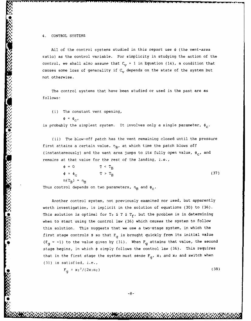
4. CONTROL SYSTEMS

All of the control systems studied in this report use 0 (the vent-area

ratio) as the control variable. For simplicity in studying the action of the

control, we shall also assume that Cv = 1 in Equation (14), a condition that

causes some loss of generality if Cv depends on the state of the system but

not otherwise.

The control systems that have been studied or used in the past are as

follows:

(i) The constant vent opening,

(P = Oc'

is probably the simplest system. It involves only a single parameter, Oc"

(ii) The blow-off patch has the vent remaining closed until the pressure

first attains a certain value, 9B' at which time the patch blows off

(instantaneously) and the vent area jumps to its fully open value, 0c' and

remains at that value for the rest of the landing, i.e.,

0 = 0 T < TB

0# = Oc T > TB (37)

• n(TB ) = 9B

Thus control depends on two parameters, 9B and 0c.

Another control system, not previously examined nor used, but apparently

5. worth investigation, is implicit in the solution of equations (30) to (36).

* This solution is optimal for To 1 T 1 Tf, but the problem is in determining

when to start using the control law (36) which causes the system to follow

this solution. This suggests that we use a two-stage system, in which the

first stage controls 0 so that Fg is brought quickly from its initial value

* (Fg = -1) to the value given by (31). When F attains that value, the second

stage begins, in which 0 simply follows the control law (36). This requires

that in the first stage the system must sense Fg, xi and X2 and switch when

(31) is satisfied, i.e.,

* Fg = X2 2 /(2xia2) (38)

-8-

xi aid X2 can be calculated by sensing Fg and performing numerical integration

of (12) and (13), so that only Fq really has to be acquired.

However, another question is whether this control system can respond

quickly enough so that 0 will be set "instantaneously" (i.e. in negligible

time) to the value demanded by (36). Alternatively, can 0 be controlled in

the first stage so that it will both (a) pressurize the bag enough to cause

(31) to be satisfied at some To and (b) have the value demanded by (36) at

that To?

It is not clear whether these difficulties can be surmounted in practice

without making the system distastefully complicated. Aiso, when this system

is in the second stage, the automatic control is of open loop type, i.e., it

makes no use of information about F or any of the stated variables. The same

i* is true of the constant vent opening. The blow-off patch is affected by the

system state only to the extent of being actuated when q is large enough. To

some degree, therefore, these systems all share the usual shortcomings of open

loop control, in particular they may not function well if subject to unknown

or random fluctuations of input.

Accordingly, an entirely different control system was investigated in this

study. Since measurements of F are the easiest ones to obtain, the system

was defined by

DO : P2Fg - PI = P2(F -r), r = PI/P2 (39)

and

dO/dT = D if D > 0 or 0 > 0 (39)

= = C if D 0 and O = 0 (39)

y where the parameters Pi and P2 have to be chosen so that the system is brought

to x1 = X2 = 0. This system is conceptually very simple; the vent is openedor closed at a rate proportional to F g-r.

0 -9-

'tv 5. NUMERICAL ANALYSIS OF LANDINGS WITH CONTROLS

In order to investigate the behavior of the control systems described in

% Section 4, a computer program was written that carries out the numerical

integration of the differential equation systems (12) to (16) and (19) to

(23). This program is listed in Appendix A. It consists of a main program,

MAIN, which reads the physical parameters, forms the dimensionless quantities

al, M2, a3, and

a4 = r ,

and invokes the IMSL routine DVERK to do the numerical integration. After

completing the solution, MAIN writes the results for xi, X2, X3,

X4

and F in file 7 and the derivatives, dxj/dT (j = 1,..., 4), in file 8.

The routine DVERK uses a Range-Kutta integration scheme which requires

that the user furnish a subroutine, FCN, for evaluating each dxj/dT, given the

. values of the time and all the xj. The control system is modelled by a set of

instructions in this subroutine which define x4 = 0 or dx4/dT = do/dT.

We adopted the parameters given in Table 2 as a standard condition and for

this condition explored the behavior of the three control systems described

earlier, recalling that the objectives are to bring the system from the

initial point

x1 =i, X2 = -1, X3 =1

% to the final point

Xl = X2 = 0

* and to do so as smoothly as possible in the sense that the maximum of Fg

d iring the motion should be as small as possible.

The simplest control system is that with constant vent opening,

or

dx,./dT =0 and X4.(0)

* With this single parameter it was impossible to attain the final point

X1 = X2 0. The "best" results (best in the sense described below) were

-10-0

4

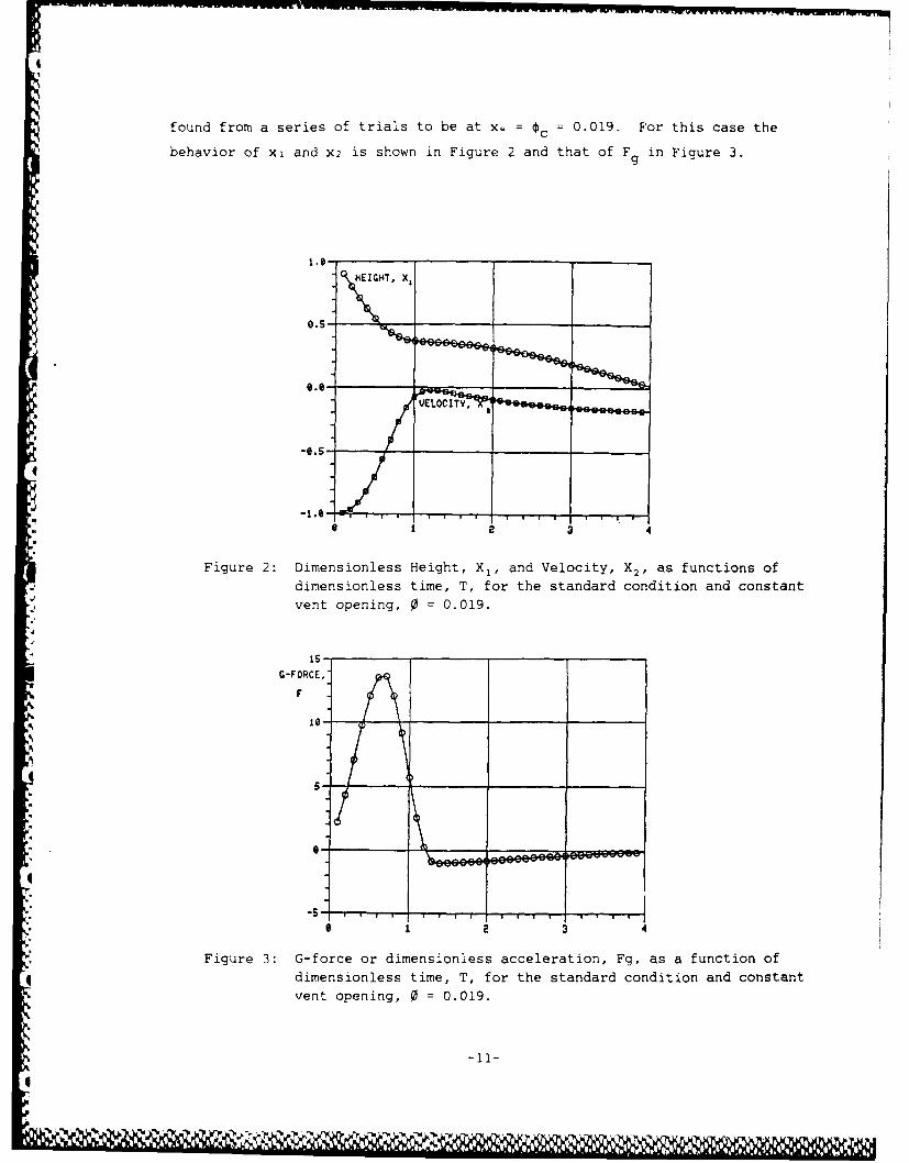
found from a series of trials to be at x. =c = 0.019. For this case the

behavior of xi and x2 is shown in Figure 2 and that of Fg in Figure 3.

3

Figure 2: Dimensionless Height, X1 , and Velocity, X2, as functions ofdimensionless time, T, for the standard condition and constantvent opening, 0 = 0.019.

Is

G-FORCEfF

0 3 4

Figure 3: G-force or dimensionless acceleration, Fg, as a function ofdimensionless time, T, for the standard condition and constantvent opening, 0 = 0.019.

-11-

4

-p

The system has X2 0 when 1.0 < T < 1.5, but xi = .36 at that time.

After almost coming to rest the system gradually resumes its descent until it

strikes the ground (i.e., xi = 0) with velocity X2= -.18 at time T t 4.1.

During this second phase of the landing, the pressure of the air in the bag is

not great enough to equilibrate the load, so F is slightly negative. If

X4 = Oc > 0.019, i.e., the vent is opened wider than the optimal value, the

load strikes the ground earlier and with higher velocity. For example, if

Oc =0.025, the load lands when T = 2.17 with X2 t -.25. On the other hand if

(c < 0.019, the vent is narrower than the optimal value, the load bounces off

the bag and accuracy of Equations (18) to (20) is thereafter doubtful.

Moreover, the maximum F values are higher in this case than the others.

For example

c = .015 causes max Fg = 16

c = .019 causes max Fg = 14

'Oc = .025 causes max Fg = 9

To summarize, this simple control cannot steer this system to the origin.

At best it will land this system with velocity X2 = -.18 and max F. = 14.

The blow-off patch control system was examined next. Control now depends

on two parameters

)B = blow-off pressure (in atmospheres)

c= dimensionless vent area.

A number of cases were run for various values of these two parameters.

The results were qualitatively like those for the previous constant vent

* control, in that the system could not be steered to the point xi = x2 = 0 by

the control. Instead the system attained x2 = 0 at height xi, (i.e. it paused

at height xi) and then eventually attained xi = 0 at a velocity x2, just asfor the constant vent case. The "best" results are listed in Table 3.

-12-

V

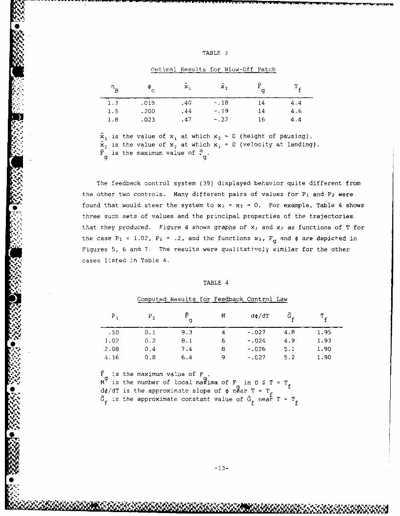
TABLE 3

Optimal Results for Blow-Off Patch

" k2F TB C g f

1.3 .019 .40 -.18 14 4.41.5 .200 .44 -.19 14 4.61.8 .023 .47 -.22 16 4.4

Kx is the value of xi at which x2 = 0 (height of pausing).x2 is the value of x2 at which x i = 0 (velocity at landing).F is the maximum value of f .

g g

The feedback control system (39) displayed behavior quite different from

the other two controls. Many different pairs of values for Pi and P2 were

found that would steer the system to xi = x2 = 0. For example, Table 4 shows

three such sets of values and the principal properties of the trajectories

that they produced. Figure 4 shows graphs of x, and x2 as functions of T for

* the case Pi = 1.02, P2 = .2, and the functions X3, Fg and 0 are depicted in

Figures 5, 6 and 7. The results were qualitatively similar for the other

*, cases listed in Table 4.

TABLE 4

Computed Results for Feedback Control Law

Pi P2 P M do/dT G Tf

.50 0.1 9.3 4 -.027 4.8 1.95

1.02 0.2 8.1 6 -.024 4.9 1.93

2.08 0.4 7.4 8 -.026 5.1 1.904.16 0.8 6.4 9 -.027 5.2 1.90

F is the maximum value of FM is the number of local mauima of F in 0 - T =Tf

* do/dT is the approximate slope of 0 n~ar T = Tf

f is the approximate constant value of Gf near T = Tf

-13-

#

The principal feature of these results is the oscillation in Fg, X3 and 0,

an oscijlation which is mildly discernible also in the plot of X2 but not of

xi. A perturbation analysis of the differential-equation system is done in

Appendix B to show the origins of this behavior. However, it is clear that

the F values obtained with this control are much lower than with either of

the other controls. A practical question is whether the control system can

respond quickly enough to enforce the control law during an oscillation of

this type.

4.8

STIIME, T

Figure 4: Dimensionless Height, X1 , and Velocity, X2 as Functions of

-. Dimensionless Time, T, for the Standard Condition,Feedback Control with P, 1.02, P2 = 0.20 and T Z 1.0.

V,.

_ -14-

-L. " "Ne F I4,6 N.

DENSITY,

0.0. .4 4.1 0 .1 1.4TIR~E,

Figure 5a: Dimensionless Air Density in Bag, X., as a Function of0Dimensionless Time, T, for the Standard Condition,

Feedback Control with P, 1.02, P2 0.20 and T 9 1.0.

A1..

DE NSITY

-. 1.U3A1

1.14-

Figure 5b: Dimensionless Air Density in Bag, X3, as a Function ofDimensionless Time, T, for the Standard Condition,Feedback Control with P, 1.02, P2 =0.20 and T k 1.0.

Ile5

4 04-FORCE.FS g_ AM,

4-

.l 6.3 p 6.4 6.6 .3 a..?IRE, 7

Figure 6a: G-force as a Function of Dimensionless Time, T, for the

Standard Condition, Feedback Control with P = 1.02,

P 2 = 0.20 and T _ 1.0.

" F

3..-• 4.3.

1.6 1. 1.4 1.6 1.3 1.0

TIE. T

Figure 6b: G-force as a Function of Dimensionless Time, T, for the

Standard Condition, Feedback Control with P1 1.02,

P2 = 0.20 and T . 1.0.

-16-

VENT AAEA.

6.04-

6 ~ .1 1.4 6.6 1.1 1.0

TIM~E, T

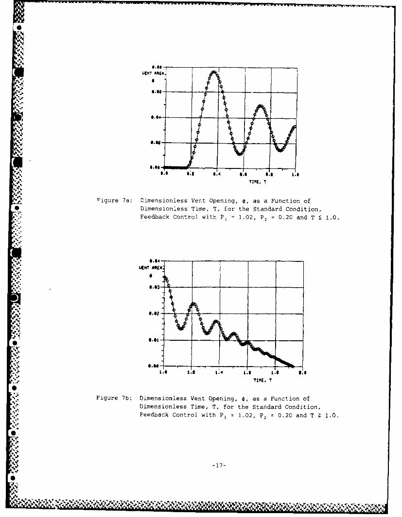
Pigure 7a: Dimensionless Vent Opening, 0, as a Function of* Dimensionless Time, T, for the Standard Condition,

Feedback Control with P, = 1.02, P 2 = 0.20 and T 1.0.

0.04-VJENT? AREA;

04.03

a..3

TIME, T

Figure 7b: Dimensionless Vent Opening, , as a Function of

Dimensionless Time, T, for the Standard Condition,Feedback Control with P, = 1.02, P2 = 0.20 and T Z 1.0.

-17-

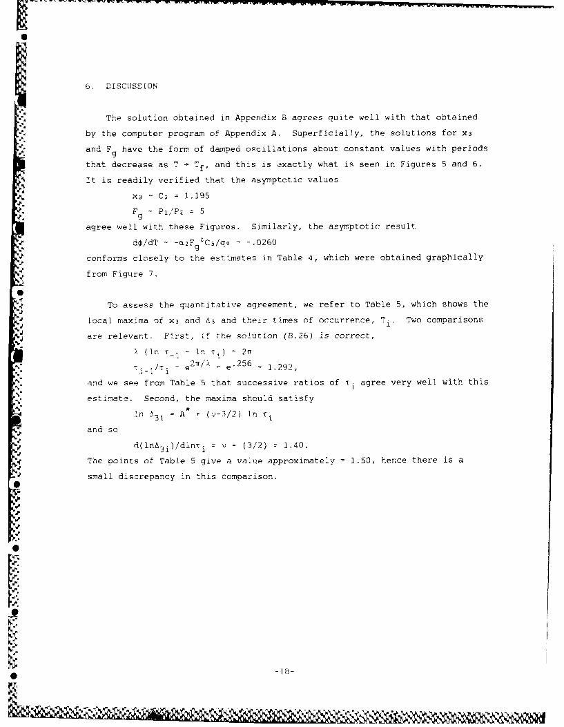
6. DISCUSSION

The solution obtained in Appendix B agrees quite well with that obtained

by the computer program of Appendix A. Superficially, the solutions for X3

and Fg have the form of damped oscillations about constant values with periods

that decrease as T - Tf, and this is exactly what is seen in Figures 5 and 6.

It is readily verified that the asymptotic values

X3 ~ C 3 = 1.195

F 9 Pi'/P2 =5

agree well with these Figures. Similarly, the asymptotic result

d /dT - -O2F gC3/qQ = -.0260

conforms closely to the estimates in Table 4, which were obtained graphically

from Figure 7.

To assess the quantitative agreement, we refer to Table 5, which shows the

j local maxima Of X3 and A3 and their times of occurrence, T1 . Two comparisons

are relevant. First, if the solution (B.26) is correct,

X (In -1 - In Ti) 21

T i i = e 2 T/ X/ = e' 256 = 1.292,

and we see from Table 5 that successive ratios of i agree very well with this4"

estimate. Second, the maxima should satisfy

In A3i = A + (v-3/2) In Ti

and so

d(lnA3i)/dln i = v - (3/2) = 1.40.

The points of Table 5 give a value approximately 1.50, hence there is a

small discrepancy in this comparison.

-

A. TABLE 5

CscbLat ion Extremes for Feedback Control Law

T x T - T. T /. A3 in " .I i f i I i+1 3

.2b5 1.665 1.296 .099 -2.31 .510

.645 1.285 1.298 .065 -2.73 .251

.940 .990 i.303 .044 -3.12 -.010

1.170 .760 1.288 .030 -3.51 -.274

1.340 .590 1.297 .020 -3.91 -.5281.475 .455 1.319

1.585 .345 1.302

1.665 .265

V, Two possible sources of error in the estimate of Appendix B are these:

(i) The series expansions involved in obtaining Equations (B.10), (B.11)

and (B.12) are not extremely accurate.

(ii) The estimate (B.23) is only a moderately accurate approximation to

V the solution of (B.22).

It is questionable whether the effort involved in improving these

approximations is worth the trouble.

Several other comments can be made about this solution.

(a) The differential equation (B.25) has a singularity at T = 0, T Tf

that casts doubt upon the correctness of the limiting behavior of the

solution, (B.26), a s Tf.

(b) The fact that F - PI/P 2 furnishes a fairly accurate solution of

(B.22) suggests that the zero-th order solutions are not very sensitive to the

values of Pi and P2 separately, but only to the ratio of PI/P 2, a conclusion

supported by the numerical results in Table 4. However, the perturbation

solution (B.27) depends strongly on X, which depends on a and so is influenced

by P2 alone (see (B.20)). As P2 increases, X increases and the solutions

-19-

% -

; .,,, ,:< < - ': .'','v,.-:' . -',2 . ",a"-,, . -.i ' Y,, ,-'i ' .,. .. .,,.a.;, .-v ... ,.,,:. ,,.-. . ..% v,4- ...... ..... .. ' ', ~a~w'whw,?i*,Tw .... <.......-......."B -. , , ,",, .:,' ,",,<'. , T,,,. .K ,' ¢ ,

oscillate more rapidly, a result that is confirmed by the values of M in

Table 4.

(c) A valid question about this control system is whether the control

mechanism can change the vent opening fast enough to keep up with the changes

in F We have

jdO/dTI S Ido/dTj + IdAo/dTJ

and

dOo/dT = -.026. Also, from (B.20)

IdAo/dTj IaLA3l I aIA31and from the computations, Figure 5, we see that IA 31 S 0.1.

Me Hence

fdp/dTj .026 + 6.37 x .01 = .090.

Thus

.-. dAv/dT - VABH- do/dT S 9 ft2/s

* . This rather crude estimate implies that the system must be able to change the

vent area at a rate of .009 ft2/ms in order to control the air bag in the

manner assumed by the analysis. It is not known whether this is an attainable

rate because much depends on the shape of the vent, but for any specified vent

geometry (e.g., rectangular), it should be possible to decide the question.

(d) We see from Table 4 that, as Pi and P2 increase but remain in almost

the same proportion, the maximum F decreases noticeably. This suggests that

the most effective control is obtained with Pi/P2 = 5 and P2 as large as

A possible. However, as mentioned under (b), the oscillation becomes more rapid5%4 as P2 increases. When P2 is increased, the oscillation eventually becomes so

quick that the control system cannot keep up with it, and the present analysis

becomes inaccurate. A more perceptive analysis, in which the effect of

control system response is modelled both theoretically and numerically, would

shed valuable light on the practical improvement that might be attained with a

control system of this general type.

(e) The parameter, X, that determines the frequency of the perturbation

oscillation, is rather large, eg., k A 24.5 - I in the example of Appendix B.

We see from (B.26) that the size of A depends on qo (i.e., ultimately a3), a,

and r,. While qo 24.7 is fairly iarge, a/b 23.8 is almost as large, and

%2)

0

%v.

the largeness of \ results about equally from both. In fact a is fairly large

because ai is so, and b is rather small because a2 is. Thus all three

parameters a,, a2 and O3 in the combination aci32 have substantial

.

SConcerning the two open-loop control systems, little further comment is

needed, except to remark that the numerical integration subroutine, DVERK,

experienced some convergence difficulty with the discontinuity that occurs for

the blow-off patch. The results for these computations are less accurate than

for the other control systems although not sufficiently so to alter the main

,a

-

S. A

'd. -.

N'.

-,.

.5.-2i

*5A

7. CONCLUSIONS AND RECOMMENDATIONS

The results of this preliminary study of airbag control systems are as

follows:

(i) Neither of the open loop systems performed in a wholly satisfactory

way for two reasons. They did not bring the system to the desired end point,

and the maximum G-force was very high.

'S.,

(ii) The feedback system with vent-rate proportional to the G-force was

%better on both counts than either open-loop system. For many pairs of values

of Pi and P2 it brought the system to the end point and did so with a maximum

G-force much smaller than either open loop control.

(iii) A number of questions remain about this particular control system.

It would be desirable to eliminate the oscillation or at least reduce its

5 frequency if that can be done without seriously increasing F or degrading its

ability to attain the desired end point. Also, we need to clarify the

'-. behavior near T = Tf, and it would be desirable to conduct stability studies

of this control system, i.e., how it responds to either deterministic or

-' random errors in the inputs or environment.

(iv) The results encourage us to think that closed-loop control systems

in general have much to offer in improving air-bag performance. Although the

closed-loop system studied in this report is a plausible one that may be

realizable in practice, there are many other possibilities. For example the

control law

d(P/dT =-Pi + P2F 9- P0P

may also bc realizable and, if the parameters are chosen well, have fewer

undesirable side effects than the law studied here.

(v) Concerning the computer program, the values of the control

S- parameters, Pi and P2, were found by manual trial-and-error in the present

study. It is possible to include in the program a subroutine for nonlinear

optimization, which will carry out this process "automatically". For example,

the nonlinear least-squares solver NL2SOL has a number of attractive features

-22-

for a study of this kind. However, even the best of these subroutines can

fail if the optimal solution is not unique, so much caution is required in

their use.

We recommend, therefore, that further study of both open and closed-loop

-. control systems be undertaken, with emphasis on the latter. In particular,

further study of the present control algorithm is justified, as sketched under

(iii) abiove. Other couit,- laws ought _also to be examined. If a substantial

investigation is undertaken, the computer program of Appendix A should first

be enhanced by inclusion of a carefully chosen nonlinear optimization

subroutine.

N

-. .-

0

-23

0?

, * }~~.

0

8. REFERENCES

I 1. Nykvist, William, "Balloon-skirt Airbags as Airdrop Shock Absorbers:Performance in Vertical Drops", U.S. Army Natick Research and DevelopmentCenter, Natick, MA, Technical Report No. TR82/026, Dec. 1981.

2. Patterson, Timothy, "Design, Fabrication and Testing of an AirdropPlatform Utilizing Airbags as Shock Absorbers", Northeastern University,Department of Mechanical Engineering, Master Thesis, May 1985.

3. Browning, A.C., "A Theoretical Approach to Air Bag Shock Absorber Design",

Royal Aircraft Establishment, Farnborough, England, Technical Note No.Mechanical Engineering 369, Feb. 1963.

4. Esgar, J.B. and Morgan, W.C., "Analytical Study of Soft Landings onGas-filled Bags", National Aeronautics and Space Administration, LewisResearch Center, Cleveland, OH, Technical Report No. R75, 1960.

This document reports research undertaken at the

U.S. Army Natick Research Development and EngineeringCenter and has been assigned No. NATICK/TR-88/021 inthe series of reports approved for publication.

* -24-

APPENDIX A: Computer Programs

The following pages contain listings with comments of the three elements

needed to carry out the computations described in Section 5. These elements

are presently stored in the file

BAG * FF.

on the UNIVAC 1106 at the U.S. Army Natick Research, Development and

Engineering Center. The elements are

M, the main program

FNI, the subroutine, FCN, called by DVERK

D, a typical data set.

M is listed below followed by FNI and 0. The data in D is that which produced

the output for the constant vent-opening control system in Figures 2 and 3.

PROGRAM FOR AIRBAG CONTROL

This program calculates the motion of a platform during a landing

cushioned by an airbag with an automatic control system. It is based on the

system of dimensionless equations in the report "A Preliminary Study of

Control Systems for Platform Landings Cushioned by Airbags" by E.W. Ross.

The main program, given below, reads in the physical quantities, converts

them to dimensionless parameters and then calls the IMSL subroutine DVERK,

which does numerical integration of the differential. equation system, using a

Runge-Kutta procedure. The subroutine DVERK call the user-supplied subroutine

* FCN, which calculates the derivatives, given the function values. The

instructions which define the control system are embedded in this subroutine.

.- 25-

DEFINITIONS OF PRINCIPAL QUANTITIES:

PA,RHOA,GM - pressure, mass-density and gamma for air

AB - cross-sectional area of airbag

SG - acceleration of gravity

. W - weight of platform, load and bag

VO - velocity of platform at first contact

H - height of platform at first contact

- N - number of variables in vector X (usually 4)J

TOL - accuracy threshold for DVERK

NTS - number of time steps in the integration

TI, TF - initial and final time

YI - array of initial values of the variables Y

LAM - array of integer variables for information recordingand imposing certain conditions.

CP - array of control and information paramaters

Y - array of main variables, as follows:

Y(1) = dimensionless height

Y(2) = dimensionless velocity

Y(3) = dimensionless density

Y(4) = dimensionless vent area (control variable)

DRV - array of derivatives of Y

GF - G-force (i.e., acceleration in G-units)

The calculated values of the Y's and GF are written to file no. 7 and

DRV's are written to file no. 8. A typical set of input data for use with

this program is in the element D in this file. The program graph in this file

* can be used to cause Tektronix plotting of the results stored in file 7.

_2.S.'

p -26-

COMPILER (DIAG=3)

EXTERNAL FCN

COMMON /A/ GM,AL(4) ,LAM(5) ,GF,CP(5)DRV(4)

REAL YI(4),Y(4) ,C(24),WKV(IO,1O)***** READ IN PHYSICAL AND OTHER DATA ***

READ (5,30) PA,RH-OA,GM.

READ (5,30) AB,G,W,UO,H

READ (5,30) N,TOL,NTS

PEAD (5.30) TI,TF,(YI(J),J=1,4)

READ (5,30) (LAM(K),K-I,5)

READ (5,30) (CP(J),J=1,5)

V ***** CALCULATE THE ARRAY AL (ALPHA) OF DIMENSIONLESS PARAMETERS

AL( I)=PA*AB/W

AL( 2 )=G*H/UO/UO

AL(3)=2*GM*PA/(GM-1)/RH.OA/UO/UO

WRITE (6,40) (AL(K),K=1,4)

IND~l

T=Tl

S DO 10 Jrl..N

10 Y(J)=YI(J)

DT=(TF-T)/NTS***MAIN LOOP FOR NUMERICAL INTERATION

DO 20 I=1,NTS

TS=~TI=I*DT

CALL DVERK (N,FCN,T,Y,TS,TOL,IND,C,10,WKV,IER)

WRITE (7,40) T, (Y(J),J=1,4),GF,CP(4)

WRITE (8,50) T, (DRV(J),J=1,4)

20 CONTINUE***** END OF MAIN LOOP

30 FORMAT ()40 FORMAT (7E9.4)

50 FORIMAT (F6.4,7E9.4)

END

-27

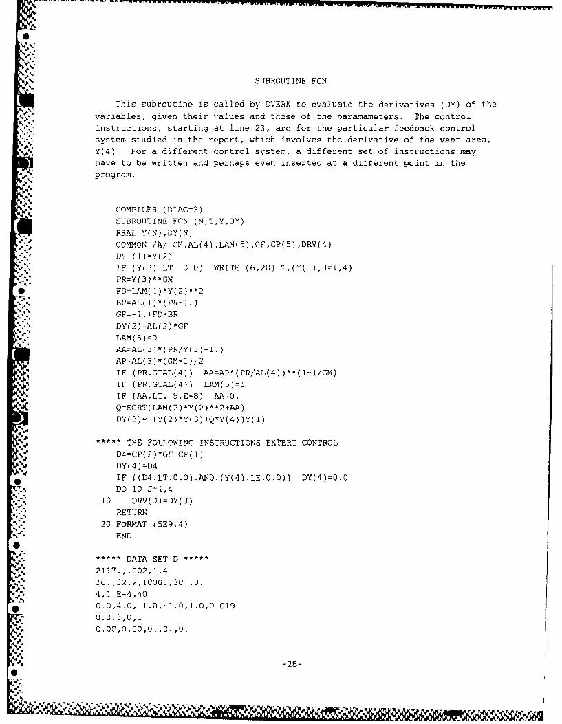
SUBROUTINE FCN

This subroutine is called by DVERK to evaluate the derivatives (DY) of the

variables, given their values and those of the paramameters. The control

instructions, starting at line 23, are for the particular feedback control

* "system studied in the report, which involves the derivative of the vent area,

Y(4). For a different control system, a different set of instructions may

have to be written and perhaps even inserted at a different point in the

a,,. program.

COMPILER (DIAG:3)

SUBROUTINE FCN (N,T,Y,DY)

REAL Y(N),DY(N)

COMMON /A/ GM,AL(4),LAM(5),GF,CP(5),DRV(4)DY (1)=Y(2)

IF (Y(3).LT. 0.0) WRITE (6,20) T,(Y(J),J=l,4)

PR=Y(3)**GM

* FD=LAM(l)*Y(2)**2" -',; BR:AL( I)*(PR-I. )

GF:-I.+FD+BR

DY(2)=AL(2)-GF

LAM(5)=O

AA=AL(3)*(PR/Y(3)-I.)

AP=AL(3 )*(GM-I )/2

IF (PR.GTAL(4)) AA:AP*(PR/AL(4))**(i- /GM)

IF (PR.GTAL(4)) LAM(5)=

N IF (AA.LT. 5.E-8) AAO.

Q=SORT(LAM( 2)*Y( 2 )**2+AA)DY(3)=-(Y(2)*Y(3)+Q*Y(4))Y(l)

***** THE FOLI-OWINr INSTRUCTIONS EXTERT CONTROL

D4=CP(2)*GF-CP(l)

DY(4)=D4

IF ((D4.LT.0.0).AND.(Y(4).LE.0.0)) DY(4)=0.0DO 10 J=1,4

: 10 DRV(J)=DY(J)

' "RETURN

20 FORMAT (5E9.4)

END

-***** DATA SET D *****

% 2117.,.002,1.4

10. , 32.2, 1000. ,30. ,3.

, 4, 1.E-4,40

I• 0.0,4.0, 1.0,-1.0,1.0,0.019

0.0.3,0,1

0.00,0.00,0.0. ,0.

"a -28-[,

APPENDIX B: Perturbation Analysis

This appendix presents a perturbation solution of the motion equations

with feedback control. This analysis is motivated primarily by the observed4.

results of the computations and secondarily by the exact, optimal solution in

Section 3 for F. = constant.

The basic set of equations is (12) to (15),(19),(22),(23) with Cv 1 and

the control law (39). The equations are then

dxl/dT = X2 ; dx2/dT = 2Fq (B.1,2)

d(xax3) = -QO ; do/dT P2F - P1 (B.3,4)Q =a32(x3 _l 1)2 (B.5)

Fg = -I + al(x 3a-l). (B.6)

We are assuming that the vent is open and the flow through it is subsonic,

hence this approximate solution is not valid initially, when the vent is

closed. Figures 5 and 6 show that for T ? 0.3 the variables xa and Fq

oscillate with decreasing amplitude about constant values, and this is the

beha--ior that we seek to explain from the above equations.

We assume that

xj - xj + Aj j = 1,2,3 (B.7)Oj =o + A0 Fg = FN 0 + AF" (B.8,9)

The quantities Aj, A0, A F are assumed to be perturbations of the zero-th order

quantities xj 0, Fg° , respectively, with A. << x 0 . Series expansions of(B.5) and (B.6) lead to

* Q q0(l + qIA3) (B.10).q0 =

L 2( [(X3°)'Y-l-l] qi = i'(y -1)(X3°) -2/ (X30)y - 1 (B.11)

F 0 al[(x 30)--I...l , A = all (X3 )Y-IA3 . (B.12)

Equation (B.12) shows that F 0 is constant if X3 0 is so. Since we

expect to obtain a solution such that x3 and Fg oscillate about constant

values, we assume0

x 3 = Ca = constant (B.13)

and so

F 0 ax(CaY 1 -I)-l. (B.14)

-29-

ELM

aThen (B.1) and (B.2) imply

I = b(T-Tf) 2 , x20 = 2b(T-Tf) (B.15)

b = ja7F 9 (B.16)

Equations (B.3) and (B.4) become, using (B.12)

d[(x j° + A)(C3 + A3)]/dT = -q(1 + qIA3 )(OO+A )

d(OO + A )/dT = P2[F g + al Y C3Y-iA3]-Pl.

The zero-order terms lead to

C3X20 -qo0o (B.17)

d~o/dT P 2F g - P, (B.18)9

and the first order terms to

d(xI0A3 )/dT = -Ca dAi/dT - qo[J + q1O0A3] (B.19)dAo/dT = aA3 , a = P2CL1 C3Y - (B.20)

Equations (B.17) and (B.15) imply

-2bCa(T-Tf)/qo (B.21)

and (B.18) becomes

- P2Fg - Pi + 2bC3/qo = 0. (B.22)

9Since Fg° and q0 all depend on C3, this is a transcendental equation for

C3 and has to be solved by trial and error.

However, we see from (B.11) that qo involves the parameter Q3 which is

very large for the present set of parameters, see Table 2. This implies that

. qo >> 1 and suggests that we attempt to solve (B.22) by neglecting the last

term, which leads to

Fg = Pl/P 2 . (B.23)

For all the values of Pi and P2 in Table 4, i.e. those values for which

X1= X2 0 at T = Tf, we have

F 9 5.

-30-

%'

This implies via (3.14), (B.11) and (B.16)

X3 C3 = [I + ( )+F I)/: 1/ 1.195

qo -24.7, QL i 2.43 and b - .268,

and we can verify that the last term in (B.22) does not greatly affect the

estimate (B.23).

These results are now used to solve (B.19) and (B.20). We can eliminateZ by differentiating (B.19) and substituting (B.20), obtaining

d2 (xI'° 3 )/dT2 qoqi4odA3/dT + C3 c 2/dT + a qoA3 + qoqiA3d~o/dT = 0.

With the aid of (B.2), (B.7) and (B.12) we find

C3d2/dT = PA3, P = a 2fC3

From (B.21)

qoqid o/dT = -2bv, V = C3qi.

Finally, if we define

4 u : X10A3 (B.24)

'.'s Sand use (B.15) we get

d 2U - 2 vK-1 du + (X2+2v)-2 u 0 (B.25)

d T 2 ciT

"5.where

T Tf - T > 0

A 2 = (aqo + 4)/b. (B.26)

Rb

.s's The numerical values of these quantities are in this case

.' v = 2.90, i = 4,08

and, for the case where P2 = .2, line 2 of Table 2,

* a = 6.37, A = 24.5.

A general solution of this equation is

u -'AT(v±) cos(a In T - S)

= pA2 + 2v - (1+2v)2/4}2 = X + 0() - I)

where A and S are the arbitrary amplitude and phase.

'-

_. The solution for A3 iS .und from (B.24) and (B.15)

A, = ATi [ - (3/ 2 ) cos(8 In T - S). (B.27)

Also A F and d6 0 /dT can be found from (B.12) and (B.20).

-31-

Yh' ,p ~

a

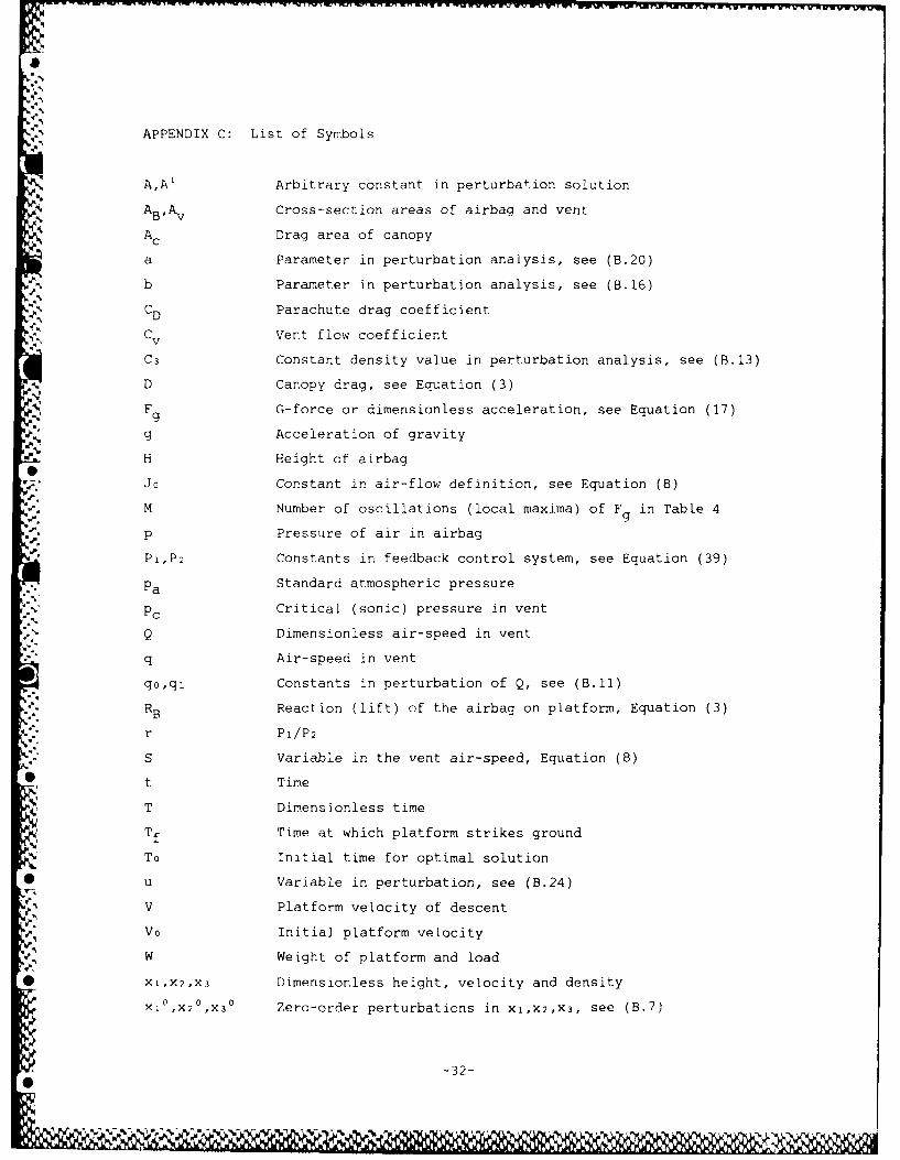
APPENDIX C: List of Symbols

A,A' Arbitrary constant in perturbation solution

A BA v Cross-section areas of airbag and vent

Ac Drag area of canopy

a Parameter in perturbation analysis, see (B.20)

b Parameter in perturbation analysis, see (B.16)

CD Parachute drag coefficient

Cv Vent flow coefficient

C3 Constant density value in perturbation analysis, see (B.13)

D Canopy drag, see Equation (3)

Fg G-force or dimensionless acceleration, see Equation (17)

g Acceleration of gravity

H Height of airbag

JO Constant in air-flow definition, see Equation (8)

M Number of oscillations (local maxima) of Fg in Table 4

p Pressure of air in airbag

PI,P2 Constants in feedback control system, see Equation (39)

Pa Standard atmospheric pressure

PC Critical (sonic) pressure in vent

Q Dimensionless air-speed in vent

q Air-speed in vent

qo,q Constants in perturbation of Q, see (B.11)

.RB Reaction (lift) of the airbag on platform, Equation (3)

.:"r PI/P2

S Variable in the vent air-speed, Equation (8)

5 t Time

T Dimensionless time

Tf Time at which platform strikes ground

To Initial time for optimal solution

* u Variable in perturbation, see (B.24)

e V Platform velocity of descent

V0 Initial platform velocity

W Weight of platform and load

* ×X,X2,X3 Dimensionless height, velocity and density

,x!0,x 0X Zero-order perturbations in xl,X2,X3, see (B.7)

-32-

v" Height of platform above ground during landing

a~a. c~. Dimensionless parameters

Constant in perturbation solution, see (B.27)

Ratio of specific heats of air

,F,A€ PPerturbations of solution, see (B.8), (B.9)

Dimensionless pressure of air in bag

r! Pressure at which blow-off patch is activated

C Critical, sonic pressure in vent

0 Energy of platform

Large parameter in perturbation oscillation, see (B.26)

Ui Constant in perturbation analysis

V Constant in perturbation analysis

0 Mass density of air in bag

D Mass density of air at standard atmospheric conditions

*C Dimensionless variable in vent flow, see Equations (18), (19)

Tf-T, see (B.26)

Dimensionless vent area, control variable

c ¢CConstant vent opening

0" Zero-th order perturbation in vent opening, see (B.8)

V

g3-

.

0

F_.'

0

: - -33 -

0