Di erential Equations and Dynamical Systems - UMass...
124
Differential Equations and Dynamical Systems Classnotes for Math 645 University of Massachusetts v3: Fall 2008 Luc Rey-Bellet Department of Mathematics and Statistics University of Massachusetts Amherst, MA 01003
Transcript of Di erential Equations and Dynamical Systems - UMass...
Differential Equations
and
Dynamical Systems
Classnotes for Math 645
University of Massachusetts
v3: Fall 2008
Luc Rey-Bellet
Department of Mathematics and Statistics
University of Massachusetts
Amherst, MA 01003
Contents
1 Existence and Uniqueness 41.1 Introduction . . . . . . . . . . . . . . . . . . . . . . . . . . . . . . . . . 41.2 Banach fixed point theorem . . . . . . . . . . . . . . . . . . . . . . . . 71.3 Existence and uniqueness for the Cauchy problem . . . . . . . . . . . . 121.4 Peano Theorem . . . . . . . . . . . . . . . . . . . . . . . . . . . . . . . 161.5 Continuation of solutions . . . . . . . . . . . . . . . . . . . . . . . . . . 191.6 Global existence . . . . . . . . . . . . . . . . . . . . . . . . . . . . . . . 211.7 Wellposedness and dynamical systems . . . . . . . . . . . . . . . . . . . 261.8 Exercises . . . . . . . . . . . . . . . . . . . . . . . . . . . . . . . . . . . 29
2 Linear Differential Equations 372.1 General theory . . . . . . . . . . . . . . . . . . . . . . . . . . . . . . . 372.2 The exponential of a linear map A . . . . . . . . . . . . . . . . . . . . 422.3 Linear systems with constant coefficients . . . . . . . . . . . . . . . . . 482.4 Stability of linear systems . . . . . . . . . . . . . . . . . . . . . . . . . 562.5 Floquet theory . . . . . . . . . . . . . . . . . . . . . . . . . . . . . . . 612.6 Linearization . . . . . . . . . . . . . . . . . . . . . . . . . . . . . . . . 652.7 Exercises . . . . . . . . . . . . . . . . . . . . . . . . . . . . . . . . . . . 70
3 Stability analysis 773.1 Stability of critical points of nonlinear systems . . . . . . . . . . . . . . 773.2 Stable and unstable manifold theorem . . . . . . . . . . . . . . . . . . 843.3 Center manifolds . . . . . . . . . . . . . . . . . . . . . . . . . . . . . . 903.4 Stability by Liapunov functions . . . . . . . . . . . . . . . . . . . . . . 933.5 Gradient and Hamiltonian systems . . . . . . . . . . . . . . . . . . . . 98
3.5.1 Gradient systems . . . . . . . . . . . . . . . . . . . . . . . . . . 983.5.2 Hamiltonian systems . . . . . . . . . . . . . . . . . . . . . . . . 100
4 Poincare-Bendixson Theorem 1064.1 Limit sets and attractors . . . . . . . . . . . . . . . . . . . . . . . . . . 1064.2 Poincare maps and stability of periodic solutions . . . . . . . . . . . . . 108
2
CONTENTS 3
4.3 Bendixson criterion . . . . . . . . . . . . . . . . . . . . . . . . . . . . . 1144.4 Poincare-Bendixson Theorem . . . . . . . . . . . . . . . . . . . . . . . 1144.5 Examples . . . . . . . . . . . . . . . . . . . . . . . . . . . . . . . . . . 118
Chapter 1
Existence and Uniqueness
1.1 Introduction
An ordinary differential equation (ODE) is given by a relation of the form
F (t, x, x′, x′′, · · · , x(m)) = 0 , (1.1)
where t ∈ R, x, x′, · · · , x(m) ∈ Rn and the function F is defined on some open set ofR×Rn × · · · ×Rn. A function x : I → Rn, where I is an interval in R, is a solutionof (1.1) if x(t) is of class Cm (i.e., m-times continuously differentiable) and if
F (t, x(t), x′(t), x′′(t), · · · , x(m)(t)) = 0 for all t ∈ I . (1.2)
We say that the ODE is of order m if the maximal order of the derivative occurring in(1.1) is m.
Example 1.1.1 Clairaut equation (1734) Let us consider the first order equation
x− tx′ + f(x′) = 0 , (1.3)
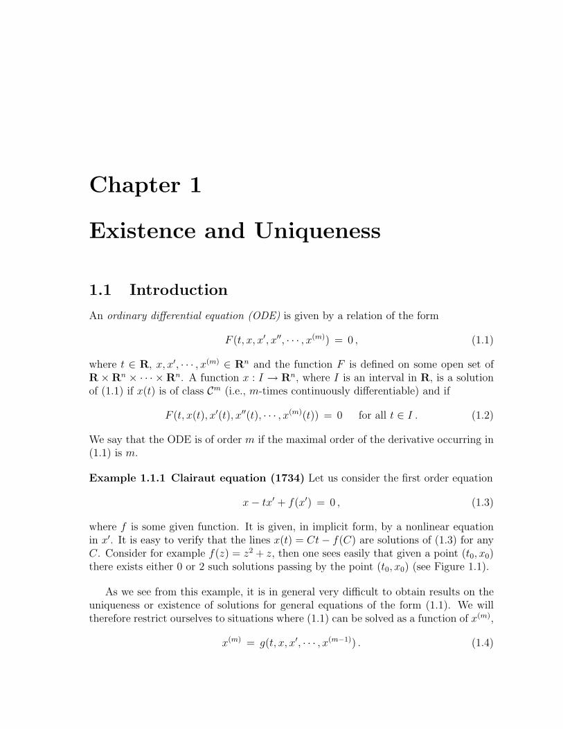
where f is some given function. It is given, in implicit form, by a nonlinear equationin x′. It is easy to verify that the lines x(t) = Ct− f(C) are solutions of (1.3) for anyC. Consider for example f(z) = z2 + z, then one sees easily that given a point (t0, x0)there exists either 0 or 2 such solutions passing by the point (t0, x0) (see Figure 1.1).
As we see from this example, it is in general very difficult to obtain results on theuniqueness or existence of solutions for general equations of the form (1.1). We willtherefore restrict ourselves to situations where (1.1) can be solved as a function of x(m),
x(m) = g(t, x, x′, · · · , x(m−1)) . (1.4)
CHAPTER 1. EXISTENCE AND UNIQUENESS 5
Figure 1.1: Some solutions for Clairault equation for f(z) = z2 + z.
Such an equation is called an explicit ODE of order m. One can always reduce anODE of order m to a first order ODE for a vector in a space of larger dimension. Forexample we can introduce the new variables
x1 = x , x2 = x′ , x3 = x′′ · · · , xm = x(m−1) , (1.5)
and rewrite (1.4) as the system
x′1 = x2 ,
x′2 = x3 ,... (1.6)
x′m−1 = xm ,
x′m = g(t, x1, x2, · · · , xm) .
This is an equation of order 1 for the supervector x = (x1, · · · , xm) ∈ Rnm (each xi isin Rn) and it has the form x′ = f(t, x). Therefore, in general, it is sufficient to considerthe case of first order equations (m=1).
If f does not depend explicitly on t, i.e., f(t, x) = f(x), the ODE x′ = f(x) iscalled autonomous. The function f : U → Rn, where U is an open set of Rn, defines avector field. A solution of x′ = f(x) is then a parametrized curve x(t) which is tangentto the vector field f(x) at any point, see figures 1.2 and (1.3).
Note a non-autonomous ODE x′ = f(t, x) with x ∈ Rn can be written as anautonomous ODE in Rn+1 by setting
y =
(xt
)y′ =
(x′
t′
)=
(f(t, x)
1
)≡ F (y) . (1.7)
CHAPTER 1. EXISTENCE AND UNIQUENESS 6
Example 1.1.2 Predator-Prey equation Let us consider the equation
x′ = x(α− βy) , y′ = y(γx− δ) , (1.8)
where α, β, γ, δ are given positive constants. Here x(t) is the population of the preysand y(t) is the population of the predators. If the population of predators y is belowthe threshold α/β then x is increasing while if y is above α/β then x is decreasing.The opposite holds for the population y. In order to study the solutions, let us dividethe first equation, by the second one and consider x as a function of y. We obtain
dx
dy=
x
y
(α− βy)
(γx− δ)or
(γx− δ)x
dx =(α− βy)
ydy . (1.9)
Integrating givesγx− δ log x = α log y − βy + Const. (1.10)
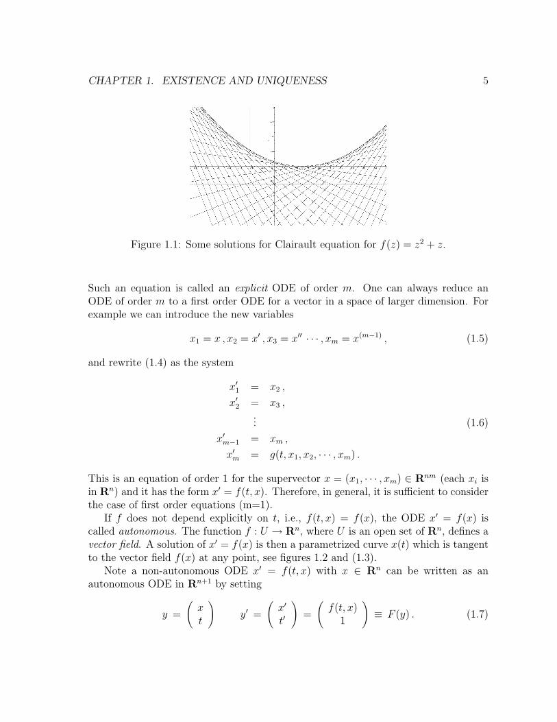
One can verify that the level curves (1.10) are closed bounded curves and each solution(x(t), y(t)) stays on a level curve of (1.10) for any t ∈ R. This suggests that thesolutions are periodic (see Figure 1.2).
Figure 1.2: The vector field for the predator-prey equation with α = 1, β = 2, γ = 3,δ = 2 and the solutions passing through the point (1, 1) and (0.5, 0.5).
Example 1.1.3 van der Pol equation. The van der Pol equation
x′′ = ε(1− x2)x′ − x . (1.11)
CHAPTER 1. EXISTENCE AND UNIQUENESS 7
It can written as a first order system by setting y = x′
x′ = y ,
y′ = ε(1− x2)y − x . (1.12)
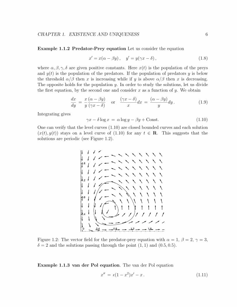
It is a perturbation of the harmonic oscillator (ε = 0) x′′ + x = 0 whose solutions arethe periodic solution x(t) = A cos(t − φ) and y(t) = x′(t) = −A sin(t − φ) (circles).When ε > 0 one observes that one periodic solution survives which is the deformationof a circle of radius 2 and all other solution are attracted to this periodic solution (limitcycle), see Figure 1.3.
Figure 1.3: The vector field for the van der Pol equation with ε = 0.1 as well as twosolutions passing through the points (.1, .2) and (2, 3).
We will discuss these examples in more details later. For now we observe that, inboth cases, the solutions curves never intersect. This means that there are never twosolutions passing by the same point. Our first goal will be to find sufficient conditionsfor the problem
x′ = f(t, x) , x(t0) = x0 , (1.13)
to have a unique solution. We say that t0 and x0 are the initial values and the problem(1.13) is called a Cauchy Problem or an initial value problem (IVP).
1.2 Banach fixed point theorem
We will need some (simple) tools of functional analysis. Let E be a vector spacewith addition + and multiplication by scalar λ in R or C. A norm on E is a map‖ · ‖ : E → R which satisfies the following three properties
• N1 ‖x‖ ≥ 0 and ‖x‖ = 0 if and only if x = 0 ,
CHAPTER 1. EXISTENCE AND UNIQUENESS 8
• N2 ‖λx‖ = |λ|‖x‖ ,
• N3 ‖x+ y‖ ≤ ‖x‖+ ‖y‖ (triangle inequality) .
A vector space E equipped with a norm ‖ · ‖ is called a normed vector space.In a normed vector space E we can define the convergence of sequence {xn}. We
say that the sequence {xn} converges to x ∈ E, if for any ε > 0, there exists N ≥ 1such that, for all n ≥ N , we have ‖xn − x‖ ≤ ε.
We say that {xn} is a Cauchy sequence if for any ε > 0, there exists N ≥ 1 suchthat, for all n,m ≥ N , we have ‖xn − xm‖ ≤ ε.
Definition 1.2.1 A normed vector space E is said to be complete if every Cauchysequence in E converges to an element of E. A complete normed vector space E iscalled a Banach space.
Let ‖ · ‖ and ‖ · ‖? denote two norms on the vector space E. We say that the norms‖ · ‖ and ‖ · ‖? are equivalent if there exist positive constants c and C such that
c‖x‖ ≤ ‖x‖? ≤ C‖x‖ for all x ∈ E .
It is easy to check that the equivalence of norm defines an equivalence relation. Further-more if a Cauchy sequence for a norm ‖ · ‖ is also a Cauchy sequence for an equivalentnorm ‖ · ‖?.
Example 1.2.2 The vector space E = Rn or Cn with the euclidean norm ‖x‖2 =(∑i x
2i )
1/2 is a Banach space. Other examples of norms are ‖x‖1 =∑i |xi| or x∞ =
supi |xi|. In any case Rn or Cn equipped with any norm is a Banach space, since allnorm are equivalent in a finite-dimensional space (see exercises).
The previous example shows that for finite dimensional vector spaces the choice ofa norm does not matter much. For infinite-dimensional vector spaces the situation isvery different as the following example demonstrate.
Proposition 1.2.3 Let
C([0, 1]) = {f : [0, 1]→ Rn ; f continuous} . (1.14)
With the norm‖f‖∞ = sup
t∈[0,1]
|f(t)| . (1.15)
C([0, 1]) is a Banach space. With either of the norms
‖f‖1 =∫ 1
0|f(t)| dt , or ‖f‖2 =
(∫ 1
0|f(t)|2 dt
)1/2
, (1.16)
C([0, 1]) is not complete.
CHAPTER 1. EXISTENCE AND UNIQUENESS 9
Proof: We let the reader verify that ‖f‖1, ‖f‖2, and ‖f‖∞ are norms.Let {fn} be a Cauchy sequence for the norm ‖ · ‖∞. We have then
|fn(t)− fm(t)| ≤ ‖fn − fm‖∞ ≤ ε for all n,m ≥ N . (1.17)
This implies that, for any t, {fn(t)} is a Cauchy sequence in R which is complete.Therefore {fn(t)} converges to an element of R which we call f(t). It remains to showthat the function f(t) is continuous. Taking the limit m→∞ in (1.17), we have
|fn(t)− f(t)| ≤ ε for all n ≥ N , (1.18)
where N depends on ε but not on t. This means that fn(t) converges uniformly to f(t)and therefore f(t) is continuous.
Let us consider the sequence {fn} of piecewise linear continuous functions, wherefn(t) = 0 on [0, 1/2 − 1/n] and fn(t) = 1 on [1/2 + 1/n, 1] and linearly interpolatingin between. One verifies easily that for any m ≥ n we have ‖fn − fm‖1 ≤ 1/n and‖fn − fm‖2 ≤ 1/
√n. Therefore {fn} is a Cauchy sequence. But the limit function is
not continuous and therefore the sequence does not converge in C([0, 1]).
We have also
Proposition 1.2.4 Let X be an arbitrary set and let us consider the space
B(X) = {f : X → R ; f bounded} . (1.19)
with the norm‖f‖∞ = sup
x∈X|f(x)| . (1.20)
Then B(X) is a Banach space.
Proof: The proof is almost identical to the first part the previous proposition and isleft to the reader.
In a Banach space E we can define basic topological concepts as in Rn.
• A open ball of radius r and center a is the set Bε(a) = {x ∈ E ; ‖x− a‖ < r}.
• A neighborhood of a is a set V such that Bε(a) ⊂ V for some ε > 0.
• A set U ⊂ E is open if U is a neighborhood of each of its element, i.e., for anyx ∈ U , there exists ε > 0 such that Bε(x) ⊂ U .
• A set V ⊂ E is closed if the limit of any convergent sequence {xn} is in V .
• A set K is compact if any sequence {xn} with xn ∈ K has a subsequence whichconverges in K.
CHAPTER 1. EXISTENCE AND UNIQUENESS 10
• Let E and F be two Banach spaces and U ⊂ E. A function f : U → F iscontinuous at x0 ∈ U if for all ε > 0, there exists δ > 0 such that x ∈ U and‖x− x0‖ < δ implies that ‖f(x)− f(x0)‖ < ε.
• The map x 7→ ‖x‖ is a continuous function of E to R, since |‖x‖ − ‖x0‖| ≤‖x− x0‖ by the triangle inequality.
Certain properties which are true in finite dimensional Banach spaces are not true ininfinite dimensional Banach spaces such as the function spaces we have considered inPropositions 1.2.3 and 1.2.4. For example we show that
• The closed ball {x ∈ E ; ‖x‖ ≤ 1} is not necessarily compact.
• Two norms on a Banach space are not always equivalent.
• The theorem of Bolzano-Weierstrass which says each bounded sequence has aconvergent subsequence is not necessarily true.
• The equivalence of K compact and K closed and bounded is not necessarily true.
The proposition 1.2.3 shows that ‖ · ‖∞ and ‖ · ‖1 are not equivalent. For, if they wereequivalent, any Cauchy sequence for ‖ · ‖1 would be a Cauchy sequence ‖ · ‖∞. But wehave constructed explicitly a Cauchy sequence for ‖·‖1 which is not a Cauchy sequencefor ‖ · ‖∞. Let us consider the Banach space B([0, 1]) and let fn(t) to be equal to 1 if1/(n+1) < t ≤ 1/n and 0 otherwise. We have ‖fn‖∞ = 1 for all n and ‖fn−fm‖∞ = 1for any n,m. Therefore {fn} cannot have a convergent subsequence. This shows atthe same time, that the unit ball is not compact, that Bolzano-Weierstrass fails, andthat closed bounded sets are not necessarily compact.
Let us suppose that we want to solve a nonlinear equation in a Banach space E.Let f be a function from E to E then we might want to solve
f(x) = x find a fixed point of f . (1.21)
The next theorem will provide a sufficient condition for the existence of a fixed point.
Theorem 1.2.5 (Banach Fixed Point Theorem (1922)) Let E be a Banach space,D ⊂ E closed and f : D → E a map which satisfies
1. f(D) ⊂ D .
2. f is a contraction on D, i.e., there exists α < 1 such that,
‖f(x)− f(y)‖ ≤ α‖x− y‖ , for all x, y ∈ D . (1.22)
Then f has a unique fixed point x in D, f(x) = x.
CHAPTER 1. EXISTENCE AND UNIQUENESS 11
Proof: We first show uniqueness. Let us suppose that there are two fixed points x andy, i.e., f(x) = x and f(y) = y. Since f is a contraction we have
‖x− y‖ = ‖f(x)− f(y)‖ ≤ α‖x− y‖ (1.23)
with α < 1, this is possible only if x = y.To prove the existence we choose an arbitrary x0 ∈ D and we consider the iteration
x1 = f(x0), · · · , xn+1 = f(xn), · · ·. Since f(D) ⊂ D this implies that xn ∈ D for anyn. Let us show that {xn} is a Cauchy sequence. We have ‖xn+1 − xn‖ = ‖f(xn) −f(xn−1)‖ ≤ α‖xn − xn−1‖. Iterating this inequality we obtain
‖xn+1 − xn‖ ≤ αn‖x1 − x0‖ . (1.24)
If m > n this implies that
‖xm − xn‖ ≤ ‖xm − xm−1‖+ ‖xm−1 − xm−2‖+ · · · ‖xn+1 − xn‖≤
(αm−1 + αm−2 + · · ·αn
)‖x1 − x0‖
≤ αn
1− α‖x1 − x0‖ . (1.25)
Therefore {xn} is a Cauchy sequence since αn → 0. Since E is a Banach space, thissequence converges to x ∈ E. The limit x is in D since D is closed. Since f is acontraction, it is continuous and we have
x = limn→∞
xn+1 = f( limn→∞
xn) = f(x) , (1.26)
i.e., x is a fixed point of f .
The proof of the theorem is constructive and provides the following algorithm toconstruct a fixed point.
Method of successive approximations: To solve f(x) = x
• Choose an arbitrary x0.
• Iterate: xn+1 = f(xn).
Even if the hypotheses of the theorem are difficult to check, one might apply thisalgorithm. If the algorithm converges this gives a fixed point, although not necessarilya unique one.
Example 1.2.6 The function f(x) = cos(x) has a fixed point on D = [0, 1]. By themean value theorem there is ξ ∈ (x, y) such that cos(x) − cos(y) = sin(ξ)(y − x),thus | cos(x) − cos(y)| ≤ supt∈[0,1] | sin(t)||x − y| ≤ sin(1)|x − y|, and sin(1) < 1. Oneobserves a quite rapid convergence to the solution 0.7390 · · ·. For example we havex0 = 0, x1 = 1, x2 = 0.5403, x2 = 0.8575, x3 = 0.6542, x4 = 0.7934, x5 = 0.7013,x6 = 0.7639, · · ·.
CHAPTER 1. EXISTENCE AND UNIQUENESS 12
Example 1.2.7 Consider the Banach space C([0, 1]) with the norm ‖ · ‖∞. Let f ∈C([0, 1]) and let k(t, s) be a function of 2 variables continuous on [0, 1]× [0, 1]. Considerthe fixed point problem
x(t) = f(t) + λ∫ 1
0k(t, s)x(s) ds . (1.27)
We assume that λ is such that α ≡ |λ| sup0≤t≤1
∫ 10 |k(t, s)| ds < 1. Consider the map
(Tx)(t) = f(t) + λ∫ 1
0 k(t, s)y(s). The map T : C([0, 1]) → C([0, 1]) is well defined andone has the bound
|(Tx)(t)− Ty(t)| ≤ |λ|∫ 1
0|k(t, s)||x(s)− y(s)| ds ≤ ‖x− y‖∞|λ| sup
0≤t≤1
∫ 1
0|k(t, s)| ds .
(1.28)Taking the supremum over t on the left side gives
‖Tx− Ty‖∞ ≤ α‖x− y‖∞ , (1.29)
so that T is a contraction. Hence the Banach fixed point theorem with D = C([0, 1])implies the existence of a unique solution for (1.27). The method of successive approx-imation applies and the iteration is, y0(t) = f and
yn+1(t) = f(t) + λ∫ 1
0k(t, s)yn(s) ds . (1.30)
1.3 Existence and uniqueness for the Cauchy prob-
lem
Let us consider the Cauchy problem
x′(t) = f(t, x(t)) , x(t0) = x0 , (1.31)
where f : U → Rn (U is an open set of R × Rn) is a continuous function. In orderto find a solution we will rewrite (1.31) as a fixed point equation. We integrate thedifferential equation between t0 an t, we obtain the integral equation
x(t) = x0 +∫ t
t0f(s, x(s)) ds . (1.32)
Every solution of (1.31) is thus a solution of (1.32). The converse also holds. If x(t) isa continuous function which verifies (1.32) on some interval I, then it is automaticallyof class C1 and it satisfies (1.31).
Let I be an interval and let us define the map T : C(I)→ C(I) given by
(Tx)(t) = x0 +∫ t
t0f(s, x(s)) ds . (1.33)
CHAPTER 1. EXISTENCE AND UNIQUENESS 13
The integral equation (1.32) can then be written as the fixed point equation
(Tx)(t) = x(t) , (1.34)
i.e., we have transformed the differential equation (1.31) into a fixed point problem.The method of successive approximation for this problem is called
Picard-Lindelof iteration:
x0(t) = x0 (or any other function) ,
xn+1(t) = x0 +∫ t
t0f(s, xn(s)) ds . (1.35)
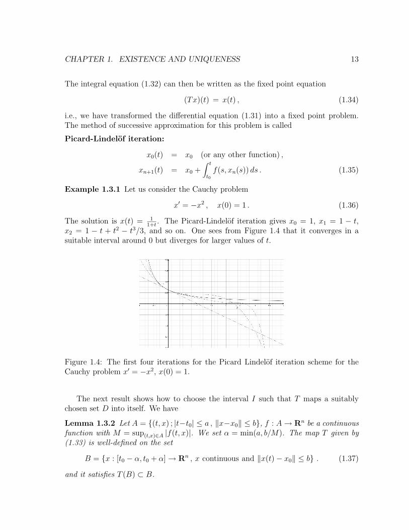
Example 1.3.1 Let us consider the Cauchy problem
x′ = −x2 , x(0) = 1 . (1.36)
The solution is x(t) = 11+t
. The Picard-Lindelof iteration gives x0 = 1, x1 = 1 − t,x2 = 1 − t + t2 − t3/3, and so on. One sees from Figure 1.4 that it converges in asuitable interval around 0 but diverges for larger values of t.
Figure 1.4: The first four iterations for the Picard Lindelof iteration scheme for theCauchy problem x′ = −x2, x(0) = 1.
The next result shows how to choose the interval I such that T maps a suitablychosen set D into itself. We have
Lemma 1.3.2 Let A = {(t, x) ; |t−t0| ≤ a , ‖x−x0‖ ≤ b}, f : A→ Rn be a continuousfunction with M = sup(t,x)∈A |f(t, x)|. We set α = min(a, b/M). The map T given by(1.33) is well-defined on the set
B = {x : [t0 − α, t0 + α]→ Rn , x continuous and ‖x(t)− x0‖ ≤ b} . (1.37)
and it satisfies T (B) ⊂ B.
CHAPTER 1. EXISTENCE AND UNIQUENESS 14
Proof: The lemma follows from the estimate
‖(Tx)(t)− x0‖ =∥∥∥∥∫ t
t0f(s, x(s)) ds
∥∥∥∥ ≤M |t− t0| ≤Mα ≤ b . (1.38)
We say that a function f : A → Rn (with A is in the previous lemma) satisfies aLipschitz condition if
‖f(t, x)− f(t, y)‖ ≤ L‖x− y‖ for all (t, x), (t, y) ∈ A . (1.39)
The constant L is called the Lipschitz constant.
Remark 1.3.3 In order to illustrate the meaning of condition (1.39), let us supposethat f(t, x) = f(x) does not depend on t and that we have ‖f(x)− f(y)‖ ≤ L‖x− y‖whenever x and y are in the closed ball Bb(x0). This clearly implies that f is continuousin Bb(x0) and f is called Lipschitz continuous. The opposite does not hold, for example
the function f(x) =√|x| is continuous but not Lipschitz continuous at 0.
If f is of class C1, then f is Lipschitz continuous. To see this consider the linez(s) = x+ s(y − x) which interpolates between x and y. We have
‖f(y)− f(x)‖ =
∥∥∥∥∥∫ 1
0
d
dsf(z(s)) ds
∥∥∥∥∥ =∥∥∥∥∫ 1
0f ′(z(s))(y − x) ds
∥∥∥∥≤ sup
z∈Bb(x0)
‖f ′(z)‖‖y − x‖ , (1.40)
and therefore f is Lipschitz continuous with L = sup{x , ‖x−x0‖≤b} ‖f′(x)‖. On the other
hand Lipschitz continuity does not imply differentiability as the function f(x) = |x|demonstrates.
The condition (1.39) requires that f(t, x) is Lipschitz continuous in x uniformly int with |t− t0| ≤ a.
If f(t, x) satisfy a Lipschitz condition we have, for any t ∈ I = [t0 − α, t0 + α],
‖(Tx)(t)− (Tz)(t)‖ ≤∫ t
t0‖f(t, x(t))− f(t, z(t))‖ dt
≤∫ t
t0L‖x(t)− z(t)‖ dt
≤ αL supt∈I‖x(t)− z(t)‖ ≤ αL‖x− z‖∞ . (1.41)
Taking the supremum over t on the left side shows that ‖Tx − Tz‖∞ ≤ αL‖x − z‖.If αL < 1 we can apply the Banach fixed point theorem to prove existence of a fixed
CHAPTER 1. EXISTENCE AND UNIQUENESS 15
point and show the existence and uniqueness for the solution of the Cauchy problemfor t in some sufficiently small interval around t0.
In fact one can omit the condition αL < 1 by applying the method of successiveapproximation directly without invoking the Banach Fixed Point Theorem. This is thecontent of the following theorem which is the basic result on existence of local solutionsfor the Cauchy problem (1.31). Here local means that we show the existence only ofx(t) is in some interval around t0.
Theorem 1.3.4 (Existence and uniqueness for the Cauchy problem) Let A ={(t, x) ; |t− t0| ≤ a , ‖x− x0‖ ≤ b} and let us suppose that f : A→ Rn
• is continuous,
• satisfies a Lipschitz condition.
Then the Cauchy problem x′ = f(t, x), x(t0) = x0 has a unique solution on I =[t0 − α, t0 + α], where α = min(a, b/M) with M = sup(t,x)∈A ‖f(t, x)‖.
Proof: We prove directly that the Picard-Lindelof iteration converge uniformly on I toa solution of the Cauchy problem. In a first step we show, by induction, that
‖xk+1(t)− xk(t)‖ ≤ MLk|t− t0|k+1
(k + 1)!for |t− t0| ≤ α . (1.42)
For k = 0, we have ‖x1(t)− x0‖ = ‖∫ tt0f(s, x(s)) ds‖ ≤M |t− t0|. Let us assume that
(1.42) holds for k − 1. Then we have
‖xk+1(t)− xk(t)‖ ≤∫ t
t0‖f(s, xk(s))− f(s, xk−1(s)‖ ds ≤ L
∫ t
t0‖xk(s)− xk−1(s)‖ ds
≤ MLk∫ t
t0
|s− t0|k
k!ds = MLk
|t− t0|k+1
(k + 1)!. (1.43)
Using (1.42), we show that {xk(t)} is a Cauchy sequence for the norm ‖x‖∞ =supt∈I ‖x(t)‖. We have
‖xk+m(t)− xk(t)‖ ≤ ‖xk+m(t)− xk+m−1(t)‖+ · · ·+ ‖xk+1(t)− xk(t)‖
≤ M
L
(Lk+m|t− t0|k+m
(k +m)!+ · · ·+ Lk+1|t− t0|k+1
(k + 1)!
)
≤ M
L
∞∑j=k+1
(Lα)j
j!, (1.44)
and the right hand side is the reminder term of a convergent series and thus goes to 0as k goes to ∞. The right hand side is independent of t so {xk} is a Cauchy sequencewhich converges uniformly to a continuous function x : I → Rn.
CHAPTER 1. EXISTENCE AND UNIQUENESS 16
To show that x(t) is a solution of the Cauchy problem we take the limit n → ∞in (1.35). The left side converges uniformly to x(t). Since f is continuous and A iscompact f(t, xk(t)) converges uniformly to f(t, x(t)) on A. Thus one can exchangeintegral and the limit and x(t) is a solution of the integral equation (1.32).
It remains to prove uniqueness of the solution. Let x(t) and z(t) be two solutionsof (1.32). By recurrence we show that
‖x(t)− y(t)‖ ≤ 2MLk|t− t0|k+1
(k + 1)!. (1.45)
We have x(t) − y(t) =∫ tt0
(f(s, x(s)) − f(s, y(s))) ds and therefore ‖x(t) − y(t)‖ ≤2M |t− t0| which (1.45) for k = 0. If (1.45) holds for k − 1 we have
‖x(t)− y(t)‖ ≤∫ t
t0L‖x(s)− y(s)‖ ds ≤ 2MLk
∫ t
t0
|s− t0|k
k!dt
≤ 2MLk|t− t0|k+1
(k + 1)!, (1.46)
and this proves (1.45). Since this holds for all k, this shows that x(t) = y(t).
1.4 Peano Theorem
In the previous section we established a local existence result by assuming a Lipschitzcondition. Simple examples show that this condition is also necessary.
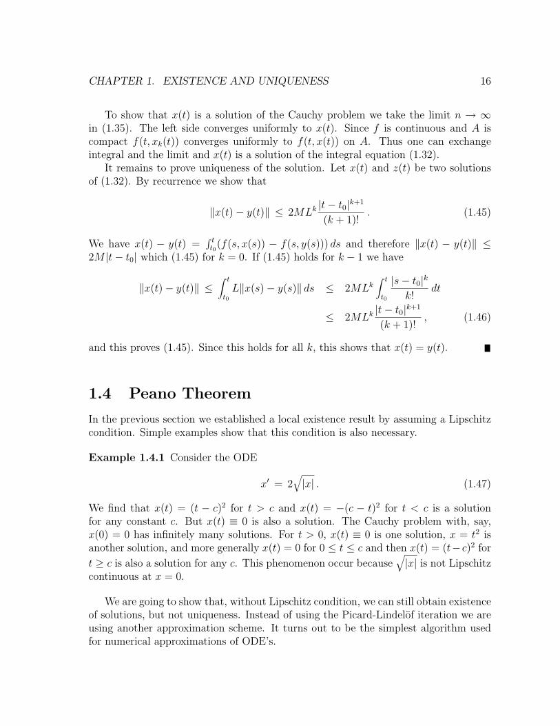
Example 1.4.1 Consider the ODE
x′ = 2√|x| . (1.47)
We find that x(t) = (t − c)2 for t > c and x(t) = −(c − t)2 for t < c is a solutionfor any constant c. But x(t) ≡ 0 is also a solution. The Cauchy problem with, say,x(0) = 0 has infinitely many solutions. For t > 0, x(t) ≡ 0 is one solution, x = t2 isanother solution, and more generally x(t) = 0 for 0 ≤ t ≤ c and then x(t) = (t− c)2 for
t ≥ c is also a solution for any c. This phenomenon occur because√|x| is not Lipschitz
continuous at x = 0.
We are going to show that, without Lipschitz condition, we can still obtain existenceof solutions, but not uniqueness. Instead of using the Picard-Lindelof iteration we areusing another approximation scheme. It turns out to be the simplest algorithm usedfor numerical approximations of ODE’s.
CHAPTER 1. EXISTENCE AND UNIQUENESS 17
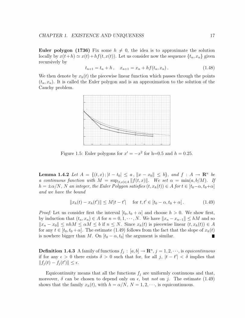
Euler polygon (1736) Fix some h 6= 0, the idea is to approximate the solutionlocally by x(t+h) ' x(t)+hf(t, x(t)). Let us consider now the sequence {tn, xn} givenrecursively by
tn+1 = tn + h , xn+1 = xn + hf(tn, xn) . (1.48)
We then denote by xh(t) the piecewise linear function which passes through the points(tn, xn). It is called the Euler polygon and is an approximation to the solution of theCauchy problem.
0 0.25 0.5 0.75 1 1.25 1.5 1.75 2 2.25 2.5
0.25
0.5
0.75
1
1.25
Figure 1.5: Euler polygons for x′ = −x2 for h=0.5 and h = 0.25.
Lemma 1.4.2 Let A = {(t, x) ; |t − t0| ≤ a , ‖x − x0‖ ≤ b}, and f : A → Rn bea continuous function with M = sup(t,x)∈A ‖f(t, x)‖. We set α = min(a, b/M). Ifh = ±α/N , N an integer, the Euler Polygon satisfies (t, xh(t)) ∈ A for t ∈ [t0−α, t0+α]and we have the bound
‖xh(t)− xh(t′)‖ ≤M |t− t′| for t, t′ ∈ [t0 − α, t0 + α] . (1.49)
Proof: Let us consider first the interval [t0, t0 + α] and choose h > 0. We show first,by induction that (tn, xn) ∈ A for n = 0, 1, · · · , N . We have ‖xn− xn−1‖ ≤ hM and so‖xn − x0‖ ≤ nhM ≤ αM ≤ b if n ≤ N . Since xh(t) is piecewise linear (t, xh(t)) ∈ Afor any t ∈ [t0, t0 +α]. The estimate (1.49) follows from the fact that the slope of xh(t)is nowhere bigger than M . On [t0 − α, t0] the argument is similar.
Definition 1.4.3 A family of functions fj : [a, b]→ Rn, j = 1, 2, · · ·, is equicontinuousif for any ε > 0 there exists δ > 0 such that for, for all j, |t − t′| < δ implies that‖fj(t)− fj(t′)‖ ≤ ε.
Equicontinuity means that all the functions fj are uniformly continuous and that,moreover, δ can be chosen to depend only on ε, but not on j. The estimate (1.49)shows that the family xh(t), with h = α/N , N = 1, 2, · · ·, is equicontinuous.
CHAPTER 1. EXISTENCE AND UNIQUENESS 18
Theorem 1.4.4 (Arzela-Ascoli 1895) Let fj : [a, b]→ Rn be a family of functionssuch that
• {fj} is equicontinuous.
• For any t ∈ [a, b], there exists M(t) ∈ R such that supj ‖fj(t)‖ ≤M(t).
Then the family {fj} has a convergent subsequence {gn} which converges uniformly toa continuous function g on [a, b].
Remark 1.4.5 As we have seen a bounded closed set in C([a, b]) is not always compact.The Arzela-Ascoli theorem shows that a bounded set of equicontinuous function is acompact set in C([a, b]) and thus it can be seen a generalization of Bolzano-Weierstrassto C([a, b]).
Proof: The subsequence is constructed proof via a trick which is referred to as ”diagonalsubsequence”. The set of rational numbers in [a, b] is countable and we write it as{t1, t2, t3, · · ·}. Consider the sequence {fj(t1)}, by assumption it is bounded in Rn
and, by Bolzano-Weierstrass, it has a convergent subsequence which we denote by{f1i(t1)}i≥1 and therefore
f11(t), f12(t), f13(t) · · · converges for t = t1 . (1.50)
Consider next the sequence {f1i(t2)}i≥1. Again, by Bolzano-Weierstrass, this sequencehas a convergent subsequence denoted by {f2i(t2)}i≥1. We have
f21(t), f22(t), f23(t) · · · converges for t = t1, t2 . (1.51)
After n steps we find a sequence {fni(t)}i≥1 of {fj(t)} such that
fn1(t), fn2(t), fn3(t) · · · converges for t = t1, t2, · · · , tn . (1.52)
Next we consider the diagonal sequence gn(t) = fnn(t). This sequence converges forany tl, since {gn(tl) = fnn(tl)}n≥l is a subsequence of {fln(tl)}n≥l which converges.
By equicontinuity, given ε > 0, there exists δ > 0 such that for all n ≥ 1, |t− t′| < δimplies that ‖gn(t)− gn(t′)‖ < ε. Let us choose rational points t1, t2, · · · tq−1 such thata = t0 < t1 < · · · < tq−1 < tq = b and ti+1 − ti < δ. For t ∈ [tl, tl+1] we have
‖gn(t)− gm(t)‖ ≤ ‖gn(t)− gn(tl)‖+ ‖gn(tl)− gm(tl)‖+ ‖gm(t)− gm(tl)‖ . (1.53)
By equicontinuity ‖gn(t) − gn(tl)‖ and ‖gm(t) − gm(tl)‖ are smaller than ε. By theconvergence of {gn(tl)} there exists N(l) such that ‖gn(tl)− gm(tl)‖ ≤ ε if n,m ≥ Nl.If we choose N = maxlNl we have that ‖gn(t) − gm(t)‖ ≤ 3ε for all t ∈ [a, b] andn,m ≥ N . This shows that gn(t) converges uniformly to some g(t) which is thencontinuous.
From this we obtain
CHAPTER 1. EXISTENCE AND UNIQUENESS 19
Theorem 1.4.6 (Peano 1890) Let A = {(t, x) ; |t− t0| ≤ a , ‖x− x0‖ ≤ b}, f : A→Rn a continuous function with M = sup(t,x)∈A ‖f(t, x)‖. Set α = min(a, b/M). TheCauchy problem (1.31) has a solution on [t0 − α, t0 + α].
Proof: Let us consider the Euler polygons with h = α/N , N = 1, 2, · · ·. The sequence isbounded since ‖xh(t)−x0‖ ≤M |t−t0| ≤Mα and equicontinuous by Lemma 1.4.2. ByArzela-Ascoli Theorem, the family xh(t) has a subsequence which converges uniformlyto a continuous function x(t) on [t0 − α, t0 + α]. It remains to show that x(t) is asolution.
Let t ∈ [t0, t0 +α] and let (tn, xn) the approximation obtained by Euler method forxh(t). If t ∈ [tl, tl+1] we have
xh(t)− x0 = hf(t0, x0) + hf(t1, x1) + · · ·+ hf(tl−1, xl−1) + (t− tl)f(tl, xl) . (1.54)
Since f(t, x(t)) is a continuous function of t it is Riemann integrable and, using aRiemann sum with left-end points have∫ t
t0f(s, x(s)) ds = hf(t0, x(t0)) + hf(t1, x(t1)) + · · ·
· · ·+ hf(tl−1, x(tl−1)) + (t− tl)f(tl, x(tl)) + r(h) , (1.55)
where limh→0 ‖r(h)‖ = 0. By the uniform continuity of f on A and the uniformconvergence of the subsequence of {xh(t)} to x(t) we have that ‖f(t, xh(t)−f(t, x(t))‖ ≤ε if h is sufficiently small (and h is such that xh belongs to the convergent subsequence).Using that xh(tj) = xj and subtracting (1.55) from (1.54) we find that
‖xh(t)− x0 −∫ t
t0f(s, x(s)) ds‖ ≤ (l + 1)hε+ ‖r(h)‖ ≤ αε+ ‖r(h)‖ (1.56)
which converges to αε as h → 0. Since ε is arbitrary x(t) is a solution of the Cauchyproblem in integral form (1.32).
1.5 Continuation of solutions
So far we only considered local solutions, i.e., solutions which are defined in a neigh-borhood of (t0, x0). Simple examples shows that the solution x(t) may not exist forall t, for example the equation x′ = 1 + x2 has solution x(t) = tan(t − c) and thissolution does not exist beyond the interval (c−π/2, c+π/2), and we have x(t)→ ±∞as t→ c± π/2.
To extend the solution we solve the Cauchy problem locally, say from t0 to t0 + αand then we can try to continue the solution by solving the Cauchy problem x′ = f(t, x)with new initial condition x(t0 + α) and find a solution from t0 + α to t0 + α+ α′, andso on... In order do this we should be able to solve it locally everywhere and we willtherefore assume that f satisfy a local Lipschitz condition.
CHAPTER 1. EXISTENCE AND UNIQUENESS 20
Definition 1.5.1 A function f : U → Rn (where U is an open set of R×Rn) satisfiesa local Lipschitz condition if for any (t0, x0) ∈ U there exist a neighborhood V ⊂ Usuch that f satisfies a Lipschitz condition on V , see (1.39).
Note that if the function f is of class C1 in U , then it satisfies a local Lipschitzcondition.
Lemma 1.5.2 Let U ⊂ R ×Rn be an open set and let us assume that f : U → Rn
is continuous and satisfies a local Lipschitz condition. Then for any (t0, x0) ∈ U thereexists an open interval Imax = (ω− , ω+) with −∞ ≤ ω− < t0 < ω+ ≤ ∞ such that
• The Cauchy problem x′ = f(t, x), x(t0) = x0 has a unique solution on Imax.
• If y : I → Rn is a solution of x′ = f(t, x), y(t0) = x0, then I ⊂ Imax and y = x|I .
Proof: a) Let x : I → Rn and z : J → Rn be two solutions of the Cauchy problemwith t0 ∈ I, J . Then x(t) = z(t) on I ∩ J . Suppose it is not true, there is point tsuch that x(t) 6= z(t). Consider the first point where the solutions separate. The localexistence theorem 1.3.4 shows that it is impossible.
b) Let us define the interval
Imax =⋃{I ; I open interval , t0 ∈ I , there exists a solution on I} . (1.57)
This interval is open and we can define the solution on Imax as follows. If t ∈ Imax,then there exists I where the Cauchy problem has a solution and we can define x(t).The part (a) shows that x(t) is uniquely defined on Imax.
Theorem 1.5.3 Let U ⊂ R×Rn be an open set and let us assume that f : U → Rn iscontinuous and satisfies a local Lipschitz condition. Then every solution of x′ = f(t, x)has a continuation up to the boundary of U . More precisely, if x : Imax → Rn isthe solution passing through (t0, x0) ∈ U , then for any compact K ⊂ U there existst1, t2 ∈ Imax with t1 < t0 < t2 such that (t1, x(t1)) /∈ K, (t2, x(t2)) /∈ K.
Remark 1.5.4 If U = R×Rn, Theorem 1.5.3 means that either
• x(t) exists for all t,
• There exists t∗ such that limt→t∗ ‖x(t)‖ =∞,
The exists globally or the solution ”blows up” at a certain point in time.
CHAPTER 1. EXISTENCE AND UNIQUENESS 21
Proof: Let Imax = (ω− , ω+). If ω+ =∞, clearly there exists a point t2 such that t2 > t0and (t2, x(t2)) /∈ K because K is bounded. If ω+ < ∞, let us assume that there exista compact K such that (t, x(t)) ∈ K for any t ∈ (t0, ω+). Since f(t, x) is bounded onthe compact set K, we have, for t, t′ sufficiently close to ω+
‖x(t)− x(t′)‖ =∥∥∥∥∫ t
t′f(s, x(s)) dt
∥∥∥∥ ≤M |t− t′| < ε . (1.58)
This shows that limt→ω+ x(t) = x+ exists and (ω+, x+) ∈ K, since K is closed. Theorem1.3.4 for the Cauchy problem with x(ω+) = x+ implies that there exists a solution in aneighborhood of ω+. This contradicts the maximality of the interval Imax. For t1 theargument is similar.
1.6 Global existence
In this section we derive sufficient conditions for global existence of solutions, i.e.,absence of blow-up for t > t0 or for all t. The following simple lemma and its variantswill be very useful.
Lemma 1.6.1 (Gronwall Lemma) Suppose that g(t) is a continuous function withg(t) ≥ 0 and that there exits constants a, b > 0 such that
g(t) ≤ a+ b∫ t
t0g(s) ds , t ∈ [t0, T ] . (1.59)
Then we haveg(t) ≤ aeb(t−t0) t ∈ [t0, T ] . (1.60)
Proof: Set G(t) = a + b∫ t
0 g(s) ds. Then G(t) ≥ g(t), G(t) > 0, for t ∈ [t0, T ], andG′(t) = bg(t). Therefore
G′(t)
G(t)=
bg(t)
G(t)≤ bG(t)
G(t)= b , t ∈ [t0, T ] , (1.61)
or, equivalently,d
dtlogG(t) ≤ b , t ∈ [t0, T ] , (1.62)
orlogG(t)− logG(0) ≤ b(t− t0) , t ∈ [t0, T ] , (1.63)
orG(t) ≤ G(0)eb(t−t0) = aeb(t−t0) , t ∈ [t0, T ] , (1.64)
which implies that g(t) ≤ aeb(t−t0), for t ∈ [t0, T ].
The first condition for global existence is rather restrictive, but it has the advantageof being easy to check.
CHAPTER 1. EXISTENCE AND UNIQUENESS 22
Definition 1.6.2 We say that the function f : R × Rn → Rn is linearly bounded ifthere exists a constant C such that
‖f(t, x)‖ ≤ C(1 + ‖x‖) , for all (t, x) ∈ R×Rn . (1.65)
Obviously if f(t, x) is bounded on R×Rn, then it is linearly bounded. The functionsx cos(x2), or x/ log(2 + |x|) are examples of linearly bounded function. The functionf(x, y) = (x+ xy, y2)T is not linearly bounded.
Theorem 1.6.3 Let f : R×Rn → Rn be continuous, locally Lipschitz (see Definition1.5.1) and linearly bounded (see Definition 1.6.2). Then the Cauchy problem x′ =f(t, x), x(t0) = x0, has a unique solution for all t.
Proof: . Since f is locally Lipschitz, there is a unique local solution x(t). We have thea-priori bound on solutions
‖x(t)‖ ≤ ‖x0‖+∫ t
t0‖f(s, x(s))‖ ds ≤ ‖x0‖+ C
∫ t
t0(1 + ‖x(s)‖) ds , (1.66)
Using Gronwall Lemma for g(t) = 1 + ‖x(t)‖, we find that
1 + ‖x(t)‖ ≤ (1 + ‖x0‖)eC(t−t0) , or ‖x(t)‖ ≤ ‖x(0)‖eC(t−t0) + (eC(t−t0)− 1) . (1.67)
This shows that the norm of the solution grows at most exponentially fast in time.From Remark 1.5.4 it follows that the solution does not blow up in finite time.
We formulate additional sufficient conditions for global existence but, for simplicity,we restrict ourselves to autonomous equations: we consider Cauchy problems of theform
x′ = f(x) , x(t0) = x0 , (1.68)
where f(t, x) does not depend explicitly on t.
Theorem 1.6.4 (Liapunov functions) Let f : Rn → Rn be locally Lipschitz. Sup-pose that there exists a function V (x) : Rn → R of class C1 such that
• V (x) ≥ 0 and lim‖x‖→∞ V (x) = ∞.
• 〈∇V (x) , f(x)〉 ≤ a+ bV (x)
Then the Cauchy problem x′ = f(x), x(t0) = x0, has a unique solution for t0 < t < +∞.
CHAPTER 1. EXISTENCE AND UNIQUENESS 23
Proof: Since f is locally Lipschitz, there is a unique local solution x(t) for the Cauchyproblem. We have
d
dtV (x(t)) =
n∑j=1
∂V
∂xj
dxjdt
= 〈∇V (x(t)) , f(x(t))〉 ≤ a+ bV (x(t) (1.69)
or, by integrating,
V (x(t)) ≤ V (x(t0)) +∫ t
t0(a+ bV (x(s)) ds . (1.70)
Applying Gronwall lemma to g(t) = a+ bV (x(t)) gives the bound
a+ bV (x(t)) ≤ (a+ bV (x(0))) eb(t−t0) . (1.71)
Therefore V (x(t)) remains bounded for all t. Since lim‖x‖→∞ V (x) = ∞, the level setsof V , V −1(c) are compact for all c and thus ‖x(t)‖ stays finite for all t > t0 too.
Remark 1.6.5 The function V in Theorem 1.6.4 is usually referred to as a Liapunovfunction. We will also use similar function later to study the stability of solutions.Note that there is no general method to construct Liapunov function, it involves sometrial and error and some a-priori knowledge on the equation.
Example 1.6.6 (Gradient systems) Let V : Rn → R be a function of class C2. Agradient systems is an ODE of the form
x′ = −∇V (x) . (1.72)
(The negative sign is a traditional convention). Note that in dimension n = 1, anyautonomous ODE x′ = f(x) is a gradient system since we can always write V (x) =∫ xx0f(y) dy.Consider the level sets of the function V , V −1(c) = {x ;V (x) = c}. If x ∈ V −1(c)
is a regular point, i.e., if ∇V (x) 6= 0, then, by the implicit function Theorem, locallynear x, V −1(c) is a smooth hypersurface surface of dimension n − 1. For example, ifn = 2, the level sets are smooth curves.
Note that if x is a regular point of the level curve V −1(c), then the solution curvex(t) is perpendicular to the level surface V −1(c). Indeed let y be a vector which istangent to the level surface V −1(c) at the point x. For any curve γ(t) in the level setV −1(c) with γ(0) = x and γ′(0) = y we have
0 =d
dtV (γ(t))|t=0 = 〈∇V (x) , y〉 , (1.73)
and so ∇V (x) is perpendicular to any tangent vector to the level set V −1(c) at allregular points of V .
We have the following
CHAPTER 1. EXISTENCE AND UNIQUENESS 24
Lemma 1.6.7 Let V : Rn → R be a function of class C2 with lim‖x‖→∞ V (x) = +∞.Then any solution of the gradient system x′ = −∇V (x), x(t0) = x0 exists for all t > t0.
Proof: If x(t) is a solution of (3.107), then we have
d
dtV (x(t)) = −〈∇V (x(t)) , ∇V (x(t))〉 ≤ 0 . (1.74)
This shows that V is a Liapunov function.
Example 1.6.8 (Hamiltonian systems.) Let x ∈ Rn, y ∈ Rn, and H : Rn×Rn →R be a function of class C2. The function H(x, y) is called a Hamiltonian function (orenergy function) and the 2n-dimensional ODE
x′ = ∇yH(x, y) , y′ = −∇xH(x, y) . (1.75)
is called the Hamiltonian equation for the Hamiltonian H(x, y). Since H is of class C2,the vector field f(x, y) = (∇yH(x, y) , −∇yH(x, y))T is locally Lipschitz so that wehave local solutions. Let (x(t), y(t)) be a solution of (1.75). We have then
d
dtH(x(t), y(t)) = ∇xH · x′ +∇yH · y′(t)
= ∇xH · ∇yH −∇yH · ∇xH = 0 . (1.76)
This means that H is a integral of the motion, for any solution H(p(t), q(t)) = constand that any solution stays on a level set of the function H. For Hamiltonian equationsthis usually referred to as conservation of energy.
Let us assume further that lim‖(x,y)‖→∞H(x, y) = ∞. This means that H(x, y) isbounded below, i.e., H(x, y) ≥ −c from some c ∈ R and that the level sets {H(x, y) =c} are closed and bounded hypersurfaces. In this case H(x, y)+c is a Liapunov functionfor the ODE (1.75) and the solution exist for all positive and negative times.
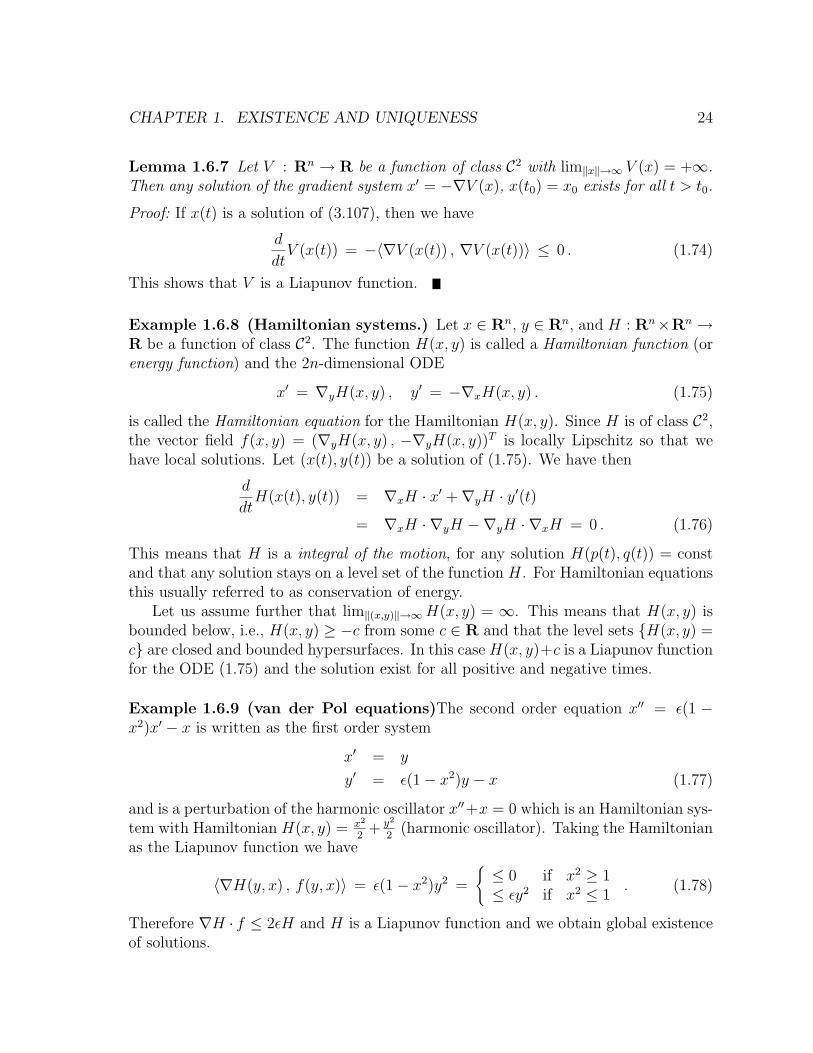
Example 1.6.9 (van der Pol equations)The second order equation x′′ = ε(1 −x2)x′ − x is written as the first order system
x′ = y
y′ = ε(1− x2)y − x (1.77)
and is a perturbation of the harmonic oscillator x′′+x = 0 which is an Hamiltonian sys-tem with Hamiltonian H(x, y) = x2
2+ y2
2(harmonic oscillator). Taking the Hamiltonian
as the Liapunov function we have
〈∇H(y, x) , f(y, x)〉 = ε(1− x2)y2 =
{≤ 0 if x2 ≥ 1≤ εy2 if x2 ≤ 1
. (1.78)
Therefore ∇H · f ≤ 2εH and H is a Liapunov function and we obtain global existenceof solutions.
CHAPTER 1. EXISTENCE AND UNIQUENESS 25
-10 -7.5 -5 -2.5 0 2.5 5 7.5 10
-5
-2.5
2.5
5
Figure 1.6: The vector field for the Hamiltonian x4−4x2+y2 and two solutions betweent = 0 and t = 3 with initial conditions (0.5, 1) and (0.5, 2.4)
Another class of systems which have solutions for all times are given by dissipativesystems.
Theorem 1.6.10 (Dissipative systems) Let f : Rn → Rn be locally Lipschitz.Suppose that there exists v ∈ Rn and positive constants a and b such that
〈f(x) , x− v〉 ≤ a− b‖x‖2 . (1.79)
Then the Cauchy problem x′ = f(x), x(t0) = x0, has a unique solution for t0 < t < +∞.
Proof: Consider the balls B0 = {x ∈ Rn ; ‖x‖2 ≤ a/b} and the Liapunov function
V (x) =||x− v||2
2. (1.80)
The condition (1.79) implies that for any solution ddtV (x(t)) ≤ 0 outside of the ball B0
and therefore V is a Liapunov function.
Remark 1.6.11 The condition (1.79) means that for the balls B = {x ∈ Rn ; ‖x −v‖2 ≤ R} with R ≥ ‖v‖+
√a/b is chosen so large that B0 is contained in the interior
of B, the vector field f points toward the interior of B. This implies that a solutionwhich starts in B will stay in B forever.
There are many variants to Theorem 1.6.10 (see the exxercises). The basic ideais to find a family of sets (large balls in Theorem 1.6.10 but the set could have othershapes) such that, on the boundary of the sets the vector f points inward. This impliesthat solutions starting on the boundary will move inward the set. If one proves thisfor all sufficiently large sets, then one obtains global existence for all initial data.
CHAPTER 1. EXISTENCE AND UNIQUENESS 26
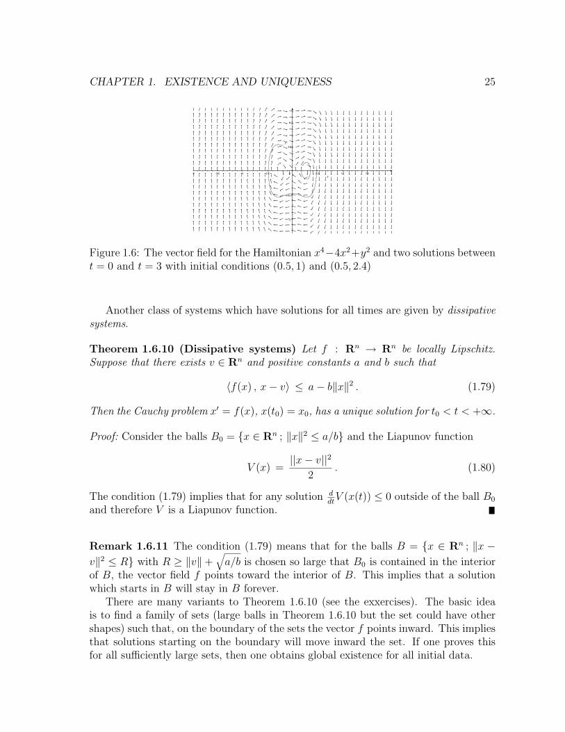
Figure 1.7: The solution for Lorentz equation with σ = 10, r = 28 and b = 83
andinitial condition (-40, 40, 25)
Example 1.6.12 The Lorentz equations are given by
x′1 = −σx1 + σx2
x′2 = −x1x3 + rx1 − x2
x′3 = x1x2 − bx3 (1.81)
Despite its apparent simplicity, the Lorentz equations exhibits, for suitable values ofthe parameters, a very complex behavior. All solutions are attracted to a compactinvariant set on which the motion is chaotic. Such an invariant set is called a strangeattractor (see Figure 1.7).
We show that the system is dissipative, we take v = (0, 0, γ). Choosing γ = b + rand using the inequality 2γx3 ≤ γ2 + x2
3, we find
〈f(x) , x− v〉 = −σx21 − x2
2 − by23 + (σ + r − γ)x1x2 + bγx3
= −σx21 − x2
2 − by23 + bγx3
≤ −σx21 − x2
2 −b
2y2
3 + bγ2
2. (1.82)
If γ = b + r, then (1.79) is satisfied with α = bγ2
2and β = min(σ, 1, b/2) and the
solution of Lorentz systems exists for all t > 0.
1.7 Wellposedness and dynamical systems
For the Cauchy problem x′ = f(t, x), x(t0) = x0, we denote the solution by x(t, t0, x0)where we explicitly indicate the dependence on the initial time t0 and the initial positionx0.
CHAPTER 1. EXISTENCE AND UNIQUENESS 27
Definition 1.7.1 The Cauchy problem x′ = f(t, x), x(t0) = x0 is called locally well-posed (resp. globally wellposed) if there exists a unique local (resp. global) solutionx(t, t0, x0) which depends continuously of (t0, x0).
Lemma 1.7.2 Let f : U → R ×Rn (U an open set of R ×Rn) be continuous andsatisfy a local Lipschitz condition. Then for any compact K ⊂ U there exists L ≥ 0such that
‖f(t, y)− f(t, x)‖ ≤ L‖x− y‖ , for all (t, x), (t, y) ∈ K (1.83)
Proof: Let us assume the contrary. Then there exists sequences (tn, xn) and (tn, yn) inK such that
‖f(tn, xn)− f(tn, yn)‖ > n‖xn − yn‖ . (1.84)
Since f is bounded on K with M = max(t,x)∈K ‖f(t, x)‖, it follows from (1.84) that
‖xn − yn‖ ≤ 2M/n . (1.85)
By Bolzano-Weierstrass, the sequence (tn, xn) has an accumulation point (t, x), andf(t, x) satisfies a Lipschitz condition in a neighborhood V of (t, x).
The bound (1.85) implies that there are infinitely many indices n such that (tn, xn) ∈V and (tn, yn) ∈ V . Then (1.84) contradicts the Lipschitz condition on V .
Theorem 1.7.3 Let f : U → R × Rn (U an open set of R × Rn) be continuousand satisfy a local Lipschitz condition. Then the solution x(t, t0, x0) of the Cauchyproblem x′ = f(t, x), x(t0) = x0 is a continuous function of (t0, x0). Moreover thefunction x(t, t0, x0) is a Lipschitz continuous function of x0, i.e., there exists a constantR = R(t) such that
‖x(t, t0, x0)− x(t, t0, x1)‖ ≤ R‖x0 − x1‖ . (1.86)
Proof: We choose a closed subinterval [a, b] of the maximal interval of existence Imax
with t, t0 ∈ [a, b]. We choose ε small enough such that the tubular neighborhood Karound the solution x(t, t0, x0),
K = {(t, x) ; t ∈ [a, b] , ‖x− x(t, t0, x0)‖ ≤ ε} , (1.87)
is contained in the open set U . By Lemma 1.7.2, f(t, x) satisfies a Lipschitz conditionon K with a Lipschitz constant L. The set V
V ={
(t1, x1) ; t1 ∈ [a, b] ‖x1 − x(t1, t0, x0)‖ ≤ εe−L(b−a)}, (1.88)
is a neighborhood of (t0, x0) which satisfies V ⊂ K ⊂ U . If (t1, x1) ∈ V we have
‖x(t, t1, x1)− x(t, t0, x0)‖ = ‖x(t, t1, x1)− x(t, t1, x(t1, t0, x0))‖
≤ ‖x1 − x(t1, t0, x0)‖+ L∫ t
t1‖x(s, t1, x1)− x(s, t1, x(t1, t0, x0))‖ . (1.89)
CHAPTER 1. EXISTENCE AND UNIQUENESS 28
From Gronwall lemma we conclude that
‖x(t, t1, x1)− x(t, t0, x0)‖ ≤ eL|t−t1|‖x1 − x(t1, t0, x0)‖ ≤ ε (1.90)
and this concludes the continuity of x(t, t0, x0). To prove the Lipschitz continuity inx0 one sets t1 = t0 in (1.90) and this prove (1.86) with R = eL|t−t0|.
This theorem shows that the Cauchy problem is locally wellposed, provided f iscontinuous and satisfy a local Lipschitz condition. If, in addition, the solutions existfor all times then the Cauchy problem is globally wellposed.
Let us consider the map φt,t0 : Rn → Rn given by
φt,t0(x0) = x(t, t0, x0) . (1.91)
The map φt,t0 maps the initial position x0 at time t0 to the position at time t, x(t, t0, x0).By definition the maps φt,t0 satisfy the composition relations
φt+s,t0(x0) = φt+s,t(φt,t0(x0)) . (1.92)
If the ODE is autonomous, i.e., f(x) does not depend explicitly on t we have
Lemma 1.7.4 (Translation property) Suppose that x(t) is a solution of x′ = f(x),then x(t− t0) is also a solution.
Proof: If x′(t) = f(x(t)), then ddtx(t− t0) = x′(t− t0) = f(x(t− t0)).
This implies that, if x(t) = x(t, 0, x0) is the solution of the Cauchy problem x′ =f(x), x(0) = x0, then x(t − t0) is the solution of the Cauchy problem x′ = f(x),x(t0) = x0. In other words x(t − t0) = x(t, t0, x0) and so the solution depends onlyon t − t0. For autonomous equations we can thus always assume that t0 = 0. In thiscase we will denote then the map φt,t0 = φt−t0,0 simply by φt−t0 . The map φt has thefollowing group properties
• (a) φ0(x) = x.
• (b) φt(φs(x)) = φt+s(x).
• (c) φt(φ−t(x)) = φ−t(φt(x)) = x.
If the solutions exists for all t ∈ R, the collection of maps φt is called the flow ofthe differential equations x′ = f(x). Note that Property (c) implies that the mapφt : Rn → Rn is invertible. More generally, a continuous map φ· : R × Rn → Rn
which satisfies Properties (a)-(b)-(c) is called a (continuous time) dynamical system.If the Cauchy problem is globally wellposed then the maps φt are a continuous flow ofhomeomorphisms and we will say that the dynamical system is continuous.
CHAPTER 1. EXISTENCE AND UNIQUENESS 29
Remark 1.7.5 If the vector fields f(t, x) are of class Ck then one would expect thatx(t, t0, x0) is also a function of class Ck. We will discuss this in the next chapter.
Remark 1.7.6 Theorem 1.7.3 shows the following: For fixed t, x(t, t0, x0) can be madearbitrarily close to x(t, t0, x0+ξ) provided ξ is small enough (depending on t!). This doesnot mean however that the solutions which start close to each other will remain closeto each other, What we proved is a bound ‖x(t, t0, x0 + ξ)−x(t, t0, x0)‖ ≤ K‖ξ‖eL|t−t0|which show that two solutions can separate, typically at an exponential rate.
Example 1.7.7 For the Cauchy problem
x′ =
(−1 00 κ
), x(0) =
(10
)(1.93)
the solution is (e−t, 0)T . The solution with initial condition (1, ξ)T is (e−t, ξeκt)T . Ifκ ≤ 0 both solutions stay a distance less than |ξ| for all time t ≥ 0, if κ > 0 the solutionsdiverge from each other exponentially with time. For given t, we can however makethem arbitrarily close up to time t by choosing ξ small enough, hence the continuity.
1.8 Exercises
1. Determine whether the following sequences of functions are Cauchy sequenceswith respect to the uniform norm ‖ · ‖∞ on the given interval I. Determine thelimit fn(x) if it exists.
(a) fn(x) = sin(2πnx) , I = [0, 1]
(b) fn(x) =xn − 1
xn + 1, I = [−1, 1].
(c) fn(x) =1
n2 + x2, I = [0, 1]
(d) fn(x) =nx
1 + (nx)2, I = [0, 1]
2. Show that ‖f‖2 is a norm on C([0, 1]).
3. Prove that all norms on Rn are equivalent by proving that any norm ‖ · ‖ in Rn
is equivalent to the euclidean norm ‖ · ‖2.Hint: (a) Let ei be the usual vector basis in Rn and write x = x1e1 + · · ·+ xnenand use the triangle inequality and Cauchy-Schwartz to show that ‖x‖ ≤ C‖x‖2.(b) Using (a) prove that | ‖x‖ − ‖y‖ | ≤ C‖x− y‖2 and thus the function ‖ · ‖ onRn with ‖‖2 is a continuous function.(c) Consider now the function ‖ · ‖ on the compact set K = {x , ‖x‖2 = 1} anddeduce from this the equivalence of the two norms.
CHAPTER 1. EXISTENCE AND UNIQUENESS 30
4. (a) Let f : U → Rn where U ⊂ Rn is an open set and suppose that f satisfiesa Lipschitz condition on U . Show that f is uniformly continuous on U .
(b) Let f : E → Rn where E ⊂ Rn is a compact set. Suppose that f is locallyLipschitz on E, show that f satisfies a Lipschitz condition on E.
(c) Show that f(x) = 1/x is locally Lipschitz but that it does not satisfy aLipschitz condition on (0, 1).
(d) Show that f(x) =√|x| is not locally Lipschitz.
(e) Does the Cauchy problem x′ = 1/x, x(0) = a > 0 have a unique solu-tion? Solve it and determine the maximal interval of existence. What is thebehavior of the solution at the boundary of this interval?
5. (a) Derive the following error estimate for the method of successive approxima-tions. Let x be a fixed point given by this method. Show that
‖x− xk‖ ≤α
1− α‖xk − xk−1‖ , (1.94)
where α is the contraction rate.
(b) Consider the function f(x) = ex/4 on the interval [0, 1]. Show that f has afixed point on [0, 1]. Do some iterations and estimate the error rigorouslyusing (a).
6. Consider the function f : R→ R given by
f(x) =
{x+ e−x/2 if x ≥ 0ex/2 if x ≤ 0
. (1.95)
(a) Show that |f(x)− f(y)| < |x− y| for x 6= y.
(b) Show that f does not have a fixed point.
Explain why this does not contradict the Banach fixed point theorem.
7. Consider the IVPx′ = x3 , x(0) = a . (1.96)
(a) Apply the Picard-Lindelof iteration to compute the first three iterationsx1(t), x2(t), x3(t).
(b) Find the exact solution and expand it in a Taylor series around t = 0. Showthat the first few terms agrees with the Picard iterates.
(c) How does the number of correct terms grow with iteration?
CHAPTER 1. EXISTENCE AND UNIQUENESS 31
8. Apply the Picard-Lindelof iteration to the Cauchy problem
x′1 = x1 + 2x2 , x1(0) = 0 (1.97)
x′2 = t2 + x1 , x2(0) = 0 (1.98)
Compute the first five terms in the taylor series of the solution.
9. Show that the assumption that ”D is closed” cannot be omitted in general in thefixed point theorem. Find a set D which is not closed and a map f : D → Esuch that f(D) ⊂ D, f is a contraction, but f does not have a fixed point in D.
10. (a) Let I = [t0 − α, t0 + α] and for a positive constant κ define
‖x‖κ = supt∈I‖x(t)‖e−κ|t−t0| .
Show that ‖ · ‖κ defines a norm and that the space
E = {x : I → Rn , x(t) continuous and ‖x‖κ <∞}
is a Banach space.
(b) Consider the IVP x′ = f(t, x), x(t0) = x). Give a proof of Theorem 1.3.4 inthe classnotes by applying the Banach fixed point theorem in the Banachspace E with norm ‖ · ‖κ for a well-chosen κ.
(c) Suppose that f(t, x) satisfy a global Lipschitz condition, i.e., there exists apositive L > 0 such that
‖f(t, x)−f(t, y)‖ ≤ L‖x−y‖ for all x, y ∈ Rn and for all t ∈ R . (1.99)
Show that the Cauchy problem x′ = f(t, x), x(t0) = x0 has a unique solutionfor all t ∈ R. Hint: Use the norm defined in (a).
11. Consider the map T given by
T (f)(x) = sin(2πx) + λ∫ 1
−1
f(y)
1 + (x− y)2dy
(a) Show that if f ∈ C([−1, 1],R) then so is T (f).
(b) Find a λ0 such that T is a contraction if |λ| < λ0 and T is not a contractionif |λ| > λ0. Hint: For the second part find a pair f, g such that ‖T (f) −T (g)‖∞ > ‖f − g‖∞.
CHAPTER 1. EXISTENCE AND UNIQUENESS 32
12. (a) Consider the norm of C([0, a]) given by
‖f‖e = max0≤t≤a
|f(t)|e−t2 . (1.100)
(Why is it a norm?) Let
Tf(t) =∫ t
0sf(s) ds . (1.101)
Show that ‖Tf‖∞ ≤ a2
2‖f‖∞ and ‖Tf‖e ≤ 1
2‖f‖e .
(b) Show that the integral equation
x(t) =1
2t2 +
∫ t
0sx(s) ds , t ∈ [0, a] , (1.102)
has exactly one solution. Determine the solution (i) by rewriting the equa-tion as an initial value problem and solving it, (ii) by using the methods ofsuccessive approximations starting with x0 ≡ 0.
13. Let us consider R2 with the norm ‖x‖ = max{|x1|, |x2|}. Let f ; R2 → R2 begiven by
f(x1, x2) =
(x2
1 + 2x22 + 5 cos(x2)
4x1x2 + 3
)(1.103)
Let K = {(x1, x2) , |x1| < 1, |x2| ≤ 2}. Find an explicit Lipschitz constant L forf on K.
14. Let f : R2 → R be of class C1 and satisfy f(0, 0) = 0. Suppose that x(t) is asolution of the ODE
x′′ = f(x, x′) , (1.104)
which is not identically 0. Show that x(t) has simple zeros. Examples: theharmonic oscillator x′′ + x = or the mathematical pendulum x′′ + sin(x) = 0.
15. Consider the initial value problem x′ = f(t, x), x(t0) = x0, where f(t, x) is acontinuous function. Show that if the initial value problem has a unique solutionthen the Euler polygons xh(t) converge to this solution.
16. Consider the Cauchy problem x′ = f(t, x), x(0) = 0, where
f(t, x) =
4sign(x)√|x| if |x| ≥ t2
4sign(x)√|x|+ 4(t− |x|
t) cos(π log t
log 2) if |x| < t2
(1.105)
The function f is continuous on R2. Consider the Euler polygons xh(t) withh = 2−i, i = 1, 2, 3, · · ·. Show that xh(t) does not converge as h → 0, computeits accumulation points, and show that they are solution of the Cauchy problem.Hint: the solutions are ±4t2.
CHAPTER 1. EXISTENCE AND UNIQUENESS 33
17. Consider the the Cauchy problem x′ = f(t, x), x(0) = 0 where f is given by
f(t, x) =
0 if t ≤ 0, x ∈ R2t if t > 0, x ≤ 0
2t− 4xt
if t > 0, 0 ≤ x < t2
−2t if t > 0, t2 ≤ x
(1.106)
(a) Show that f is continuous. What does that imply for the Cauchy problem?
(b) Show that f does not satisfy a Lipschitz condition in any neighborhood ofthe origin.
(c) Apply Picard-Lindelof iteration with x0(t) ≡ 0. Are the accumulation pointssolutions?
(d) Show that the Cauchy problem has a unique solution. What is the solution?
This problem shows that existence and uniqueness of the solution does not implythat the Picard-Lindelof iteration converges to the unique solution.
18. Consider the Cauchy problem x′ = λx, x(0) = 1, with λ > 0 and t ∈ [0, 1].Compute the Euler polygons xh(t) with h = 1/n and show that
λ
1 + λhxh(t) ≤
dxhdt
(t) ≤ λxh(t) . (1.107)
Deduce from this the classical inequality(1 +
λ
n
)n≤ eλ ≤
(1 +
λ
n
)n+λ
(1.108)
Hint: Use Gronwall Lemma.
19. Let a, b, c, and d be positive constants. Consider the Predator-Prey equationx′ = x(a − by), y′ = y(cx − d) with positive initial conditions x(t0) > 0 andy(t0) > 0. Show that the solutions exists for all t and that the solution curvesx(t), y(t) are periodic. Hint: You can use the change of variables p = log(x) andq = log(y)
20. (a) Show that any second order ODE x′′+ f(x) = 0 can be written as a Hamil-tonian system for the Hamiltonian function H(x, y) = y2/2 + V (x), wherey = x′ and V (x) =
∫ x0 f(t)dt
(b) Compute the Hamiltonian function, and it level curves and draw the solu-tions curves for the following ODE’s
i. x′′ = −ω2x (the harmonic oscillator)
CHAPTER 1. EXISTENCE AND UNIQUENESS 34
ii. x′′ = −a sin(x) (the mathematical pendulum: One end A of weightlessrod of length l is attached to a pivot, and a mass m is attached tothe other end B. The system moves in a plane under the influence ofthe gravitational force of amplitude mg which acts vertically downward.Here x(t) is the angle between the vertical and the rod and a = g/l).
iii. mr′′ = −γMm/r2 (Vertical motion of a body of mass m in free fall dueto the gravity of a body of mass M).
Depending on the energy H(x0, y0) of the initial condition discuss in detailsthe different types of solutions which can occur. Are the solutions boundedor unbounded? Are there constant solutions or periodic solutions? Do thesolutions converge as t→ ±∞?
21. (a) Consider the Hamiltonian function H(x, y) = y2/2 + V (x). Suppose thatwe have initial conditions x(0) = x0 and x′(0) = y0 > 0 with initial energyE = H(x0, y0). Use the conservation of energy to show the solution x(t) isgiven (implicitly) by the formula
t =∫ x(t)
x0
1√2(E − V (s))
ds .
(b) Assume that V (x) = V (−x), i.e., V is an even function. Show that if x(t) isa solution then so are x(c− t) and −x(t). Furthermore show that if x(c) = 0then x(c+ t) = −x(c− t) and that if x′(d) = 0 then x(d+ t) = x(d− t).
(c) Assume that V (x) = V (−x) and consider periodic solutions. We denoteby R the largest swing, i.e., the maximal positive value of x(t) along theperiodic solution. Using (a) show that the period p of the periodic solutionis given by
p = 4∫ R
0
1√2(V (R)− V (s))
ds
Hint: Consider the quarter oscillation starting at the point x(0) = 0 andy(0) = y0 > 0 and ending at x(T ) = R > 0 and y(T ) = 0. Use also thesymmetry of V and (b).
(d) Use (c) to show the period for the harmonic oscillator is independent of theenergy E.
(e) Use (c) to show that for the mathematical pendulum the period is given by
p =4√a
∫ π/2
0
1√1− k2 sin2(u)
du
where k = sin r/2. This integral is an elliptic integral of the first type. Hint:Use 1− cos(α) = sin2 α
2and the substitution sin s/2 = k sinu.
CHAPTER 1. EXISTENCE AND UNIQUENESS 35
22. Show that the following ODE’s have global solutions (i.e., defined for all t > t0).
(a)x′ = 4y3 + 2xy′ = −4x3 − 2y − cos(x)
.
(b) x′′ + x+ x3 = 0.
(c) x′′ + x′ + x+ x3 = 0.
(d)x′ = sin(2t2x)x3
1+t2+x2+y2
y′ = x2y1+x2+y2
.
(e)x′ = 5x− 2y − y2
y′ = 2y + 6x+ xy − y3 .
23. Prove the following generalizations of Gronwall Lemma.
• Let a > 0 be a positive constant and g(t) and h(t) be nonnegative continuousfunctions. Suppose that for any t ∈ [0, T ]
g(t) ≤ a+∫ t
0h(s)g(s) ds . (1.109)
Then, for any t ∈ [0, T ]
g(t) ≤ ae∫ t0h(s) ds . (1.110)
• Let f(t) > 0 be a positive function and g(t) and h(t) be nonnegative con-tinuous functions. Suppose that for any t ∈ [0, T ]
g(t) ≤ f(t) +∫ t
0h(s)g(s) ds . (1.111)
Then, for any t ∈ [0, T ]
g(t) ≤ f(t)e∫ t0h(s) ds . (1.112)
24. Consider the FitzHugh-Nagumo equation
x′1 = f1(x1, x2) = g(x1)− x2 ,
x′2 = f2(x1, x2) = σx1 − γx2 , (1.113)
where σ and γ are positive constants and the function g is given by g(x) =−x(x− 1/2)(x− 1).
(a) In the x1-x2 plane draw the graph of the curves f1(x1, x2) = 0 and f2(x1, x2) =0.
CHAPTER 1. EXISTENCE AND UNIQUENESS 36
(b) Consider the rectangles ABCD whose sides are parallel to the X1 and x2
axis with two opposite corners located on the f2(x1, x2) = 0. Show that ifthe rectangle is taken sufficiently large, a solution which start inside the rect-angle stays inside the rectangle forever. Deduce from this that the equationsfor any initial conditions x0 have a unique solutions for all time t > 0.
25. Show that the solutions of
x′1 = x1(3− 4x1 − 2x2) ,
x′2 = x2(4− 2x1 − 3x2) , (1.114)
have a unique solution for all t ≥ 0, for any initial conditions x10 , x20 wich arenonnegative. Hint: A possibility is to use a similar procedure as in the previousexercise.
26. Continuous dependence on parameters. Consider the IVP x′ = f(t, x, µ),x(t0) = x0 where f : V → Rn ( V ⊂ R×Rn ×Rk an open set). We denote byx(t, µ) the solution of the IVP (we have suppressed the dependence on (t0, x0)).Let us assume
• f is a continuous function on V .
• f(t, x, c) satisfies a local Lipschitz condition in the following sense: Given(c0, t0, x0) ∈ V and positive constants a, b, c such that A ≡ {(t, x, µ) ; |t −t0| ≤ a , ‖x − x0‖ ≤ b , ‖µ − µ0‖ ≤ c} ⊂ V then there exists a constant Lsuch that ‖f(t, x, µ)− f(t, y, µ)‖ ≤ L‖x− y‖ for all (t, x, µ), (t, y, µ) ∈ A.
Show that x(t, µ) depends continuously on µ for t in some interval J containingt0.
Chapter 2
Linear Differential Equations
We denote by L(Rn) the set of linear maps A : Rn → Rn which we identify with theset of n× n matrices A = (aij) with real entries. We write Ax instead of A(x) for thevector with coefficients (Ax)i =
∑nj=1 aijxj.
In this chapter we consider linear differential equations, i.e., ODE’s of the form
x′ = A(t)x+ g(t) , (2.1)
where x ∈ Rn, g : I → Rn, and A : I → L(Rn) with I some interval.The linear ODE is called homogeneous if g(t) ≡ 0, and inhomogeneous otherwise.
If A(t) = A is independent of t and g ≡ 0, the linear ODE x′ = Ax is called a systemwith constant coefficients.
2.1 General theory
We discuss first general properties of the differential equations x′ = A(t)x+ g(t).
Theorem 2.1.1 (Existence and uniqueness) Let I = [a, b] be an interval andsuppose that A(t) and g(t) are continuous function on I. Then the Cauchy problemx′ = A(t)x+ g(t), x(t0) = x0 (with t0 ∈ I, x0 ∈ Rn) has a unique solution on I.
Proof: The function f(t, x) = A(t)x+g(t) is continuous and satisfies a Lipschitz condi-tion on I×Rn. Therefore the solution is unique wherever it exists. Moreover on I×Rn
we have the bound ‖f(t, x)‖ ≤ a‖x‖+b where a = supt∈I ‖A(t)‖ and b = supt∈I ‖g(t)‖.Therefore we have the bound ‖x(t)‖ ≤ ‖x0‖+
∫ tt0
(a‖x(s)‖+b) ds for t0, t ∈ I. Gronwalllemma implies that ‖x(t)‖ remains bounded if t ∈ I.
Remark 2.1.2 If A(t) and g(t) are continuous on R then, applying Theorem 2.1.1 to[−T, T ] for arbitrary T shows that the solution exists for all t ∈ R.
CHAPTER 2. LINEAR DIFFERENTIAL EQUATIONS 38
Theorem 2.1.3 (Superposition principle) Let I be an interval and let A(t), g1(t),g2(t) be continuous function on I. If
x1 : I → Rn is a solution of x′ = A(t)x+ g1(t) ,
x2 : I → Rn is a solution of x′ = A(t)x+ g2(t) ,
then
x(t) := c1x1(t) + c2x2(t) : I → Rn is a solution of x′ = A(t)x+ (c1g1 + c2g2(t)) .
Proof: : This a simple exercise.
This theorem has very important consequences.
Homogeneous equations. Let us consider homogeneous Cauchy problems x′ =A(t)x, x(t0) = x0 and let denote its solutions x(t, t0, x0) to indicate explicitly thedependence on the initial data.(a) The solution x(t, t0, x0) depends linearly on the initial condition x0, i.e.,
x(t, t0, c1x0 + c2y0) = c1x(t, t0, x0) + c2x(t, t0, y0) . (2.2)
This follows by noting that, by linearity, both sides are solutions of the ODE and havethe same initial conditions. The uniqueness of the solutions implies then the equality.As a consequence there exists a linear map R(t, t0) : Rn → Rn such that
R(t, t0)x0 = x(t, t0, x0) . (2.3)
It maps the initial condition x0 at time t0 to the position at time t. The linear mapR(t, t0) is called the resolvent of the differential equation x′ = A(t)x. The i-th columnof R(t, t0) is a solution x′ = A(t)x with initial condition x0 = (0, · · · , 0, 1, 0, · · · , 0)T
where 1 is in i-th position.
(b) If x0 = 0, then x(t) ≡ 0 for all t ∈ I (The point 0 is called a critical point). As aconsequence if x(t) is a solution and it vanishes at some point t, then it is identically0.
(c) The set of solutions of x′ = A(t)x form a vector space. We call a set of solutionsx1(t), · · · , xk(t) linearly dependent if there exists constants c1, · · · , ck, with at least oneci 6= 0, such that
c1x1(t) + · · ·+ ckxk(t) = 0 . (2.4)
Note that by (b), if (2.4) holds at one point t, it holds at any point t. Therefore if theinitial condition x1(t0), · · ·xk(t0) are linearly dependent, then the corresponding solu-tions are linearly dependent for any t. The k solutions are called linearly independentif they are not linearly dependent, i.e., c1x1(t) + · · · + ckxk(t) = 0 implies that thatc1 = · · · = ck = 0.
CHAPTER 2. LINEAR DIFFERENTIAL EQUATIONS 39
(d) From (c) it follows that there exist exactly n linearly independent solutions,x1, · · · , xn. Every such set of n linearly independent solutions is called a fundamentalsystem of solutions. Any solution x of x′ = A(t)x can be written, in a unique way, asa linear combination
x(t) = a1x1(t) + · · ·+ anxn(t) . (2.5)
(e) A system of n linearly independent solutions can be arranged in a matrix Φ(t) =(x1(t), · · · , xn(t)). In this notation the i-th column of Φ(t) is the column vector xi(t).The matrix Φ(t) is called a fundamental matrix or a Wronskian for x′ = A(t)x. Itsatisfies the matrix differential equation
d
dtΦ(t) = A(t)Φ(t) . (2.6)
(f) If Φ(t) is a fundamental matrix then the resolvent is given by
R(t, t0) = Φ(t)Φ(t0)−1 . (2.7)
Indeed x(t) = Φ(t)Φ(t0)−1x0 satisfies x′ = A(t)x (because of (2.6)) and x(t0) = x0.
Theorem 2.1.4 (Properties of the resolvent) Let A(t) be continuous on the in-terval I. Then the resolvent of x′ = A(t)x satisfies
1. ∂∂tR(t, t0) = A(t)R(t, t0).
2. R(t0, t0) = I (the identity matrix).
3. R(t, t0) = R(t, t1)R(t1, t0).
4. R(t, t0) is invertible and R(t, t0)−1 = R(t0, t).
Proof: We have ∂∂tR(t, t0)x0 = ∂
∂tx(t, t0, x0) = A(t)R(t, t0)x0 and R(t0, t0)x0 = x0
for any x0 ∈ Rn. This proves 1. and 2. Item 3 simply says that x(t, t0, x0) =x(t, t1, x(t1, t0, x0)). Item 4. follows from 2. and 3. by setting t = t0.
Example 2.1.5 The harmonic oscillator x′′ + κx = 0 can be written with x1 = x andx2 = x′ as (
x1
x2
)′=
(0 1−κ 0
)(x1
x2
). (2.8)
One can find easily two linearly independent solutions, namely(cos(√κt+ φ)
−√κ sin(
√κt+ φ)
)and
(sin(√κt+ φ)√
κ cos(√κt
)(2.9)
CHAPTER 2. LINEAR DIFFERENTIAL EQUATIONS 40
By definition, the resolvent is the fundamental solution (x1(t), x2(t)) with x1(t) =(1, 0)T and x2(t0) = (0, 1)T so that we have
R(t, t0) =
(cos(√κ(t− t0)) 1√
κsin(√κ(t− t0))
−√κ sin(
√κ(t− t0)) cos(
√κ(t− t0))
). (2.10)
Note that the relation R(t, t0) = R(t, s)R(s, t0) is simply the addition formula for sineand cosine.
Theorem 2.1.6 (Liouville) Let A(t) be continuous on the interval I and let Φ(t) bea fundamental matrix of x′ = A(t)x. Then
det Φ(t) = det Φ(t0) exp(∫ t
t0traceA(s) ds
), (2.11)
where traceA(t) := a11(t) + · · ·+ ann(t).
Proof: Let Φ(t) = (φij(t))ni,j=1. From linear algebra we know that det(A) is a multilinear
function of the rows of A. It follows that
d
dtdet Φ(t) =
n∑i=1
detDi(t) where Di(t) =
φ11(t) · · · φ1n(t)...
...φ′i1(t) · · · φ′in(t)
......
φn1(t) · · · φnn(t)
. (2.12)
The matrix Di(t) is obtained from Φ(t) by replacing the i-th line by its derivative. Wehave Φ′(t) = A(t)Φ(t), i.e., φ′ij(t) =
∑nk=1 aik(t)φkj(t). Using the multilinearity of the
determinant we find
d
dtdet Φ(t) =
n∑i=1
n∑k=1
aik(t) det
φ11(t) · · · φ1n(t)...
...φk1(t) · · · φkn(t)
......
φn1(t) · · · φnn(t)
←− i− th line
=
(n∑i=1
aii(t)
)det Φ(t) . (2.13)
This is a scalar differential which can be solved by separation of variables and gives(2.11).
CHAPTER 2. LINEAR DIFFERENTIAL EQUATIONS 41
Remark 2.1.7 The Liouville theorem has the following useful interpretation. If V =(v1, · · · , vn) is a matrix whose columns are the vectors v1, · · · , vn, then | detV | is thevolume of the parallelepiped spanned by v1, · · · , vn. Using detA−1 = 1/ detA, LiouvilleTheorem is equivalent to
detR(t, t0) = exp(∫ t
t0traceA(s) ds
). (2.14)
If, at time t0 we start with a set of initial conditions B of volume, say, 1 (e.g. a unitcube), at time t the set B is mapped to a set a parallelepiped R(t, t0)B of volume
exp(∫ tt0
traceA(s) ds).
In particular, if trA(t) ≡ 0, then the flow defined by the equation y′ = A(t)ypreserves volume. We have such a situation in Example 2.1.5, see (2.8).
Inhomogeneous equations. We consider the equation
x′ = A(t)x+ g(t) . (2.15)
Theorem 2.1.8 Let x(t) be a fixed solution of the inhomogeneous equation (2.15). Ifx(t) is a solution of the homogeneous equation, then x(t) + x(t) is a solution of thehomogeneous equation and all solutions of the inhomogeneous equation are obtained inthis way.
Proof: : This is an easy exercise.
If we know how to solve the homogeneous problem, i.e. if we know the resolventR(t, t0), our task is then to find just one solution of the inhomogeneous equation. Thefollowing theorem provides an explicit formula for such solution.
Theorem 2.1.9 (Variation of constants or Duhamel’s formula) Let A(t) andg(t) be continuous on the interval I and let R(t, t0) be the resolvent of the homogeneousequation x′ = A(t)x. Then the solution of the Cauchy problem x′ = A(t)x + g(t) isgiven by
x(t) = R(t, t0)x0 +∫ t
t0R(t, s)g(s) ds . (2.16)
Proof: The general solution of the homogeneous equation has the form R(t, t0)c with c ∈Rn. The idea is to ”vary the constants” and to look for a solution of the inhomogeneousproblem of the form
x(t) = R(t, t0)c(t) . (2.17)
CHAPTER 2. LINEAR DIFFERENTIAL EQUATIONS 42
We must then have, using 1. of Theorem 2.1.4,
x′(t) =∂
∂tR′(t, t0)c(t) +R(t, t0)c′(t) = A(t)R(t, t0)c(t) +R(t, t0)c′(t)
= A(t)R(t, t0)c(t) + g(t) . (2.18)
Thusc′(t) = R(t, t0)−1g(t) = R(t0, t)g(t) , (2.19)
and, integrating, this gives c(t) = x0 +∫ tt0R(t0, s)g(s) ds. Inserting this formula in
(2.17) gives the result.
It should be noted that, in general, the computation of the resolvent for x′ = A(t)xis not easy and can rarely be done explicitly if A depends on t.
Example 2.1.10 Forced harmonic oscillator We consider the differential equationx′′ + x = f(t), or equivalently the first order system x′ = y, y′ = −x − f(t). Theresolvent is given by (2.10). The solution of the above system with initial conditions(x(0), y(0))T = (x0, y0)T is(
x(t)y(t)
)= R(t)
(x0
y0
)+∫ t
0
(f(s) sin(t− s)f(s) cos(t− s)
)ds , (2.20)
so that
x(t) = cos(t)x0 + sin(t)y0 +∫ t
0f(s) sin(t− s) ds . (2.21)
For example if f(t) = cos(√κt) we find
x(t) = cos(t)x0 + sin(t)y0 +
{ √κ
1−κ(cos(t)− cos(√κt)) κ 6= 1
12t sin(t) k = 1
. (2.22)
The motion is quasi-periodic if√κ is irrational, periodic if
√κ is rational (and 6= 1),
and the solution grows as t→∞ if κ = 1 (resonance).
2.2 The exponential of a linear map A
In this section we let K = R or C. We equip Kn with a norm, for example,
‖x‖1 =n∑i=1
|xi| , ‖x‖2 =
(n∑i=1
|xi|2)1/2
, ‖x‖∞ = max1≤i≤n
|xi| , (2.23)
then Kn is a Banach space. All norms being equivalent on Kn the choice is a matterof convenience.
CHAPTER 2. LINEAR DIFFERENTIAL EQUATIONS 43
A n× n matrix A = (aij) with aij ∈ K defines a linear map A : Kn → Kn and wedenote by L(Kn) the set of all linear maps from Kn into Kn. The set L(Kn) is alsoa vector space, of (real or complex) dimension n2 and is a Banach space if equippedwith a norm. In addition to being a vector space L(Kn) is naturally equipped withmultiplication (composition of linear maps) and it is natural and advantageous to equipL(Kn) with a norm which is compatible with matrix multiplication.
Definition 2.2.1 For A ∈ L(Kn) we define
‖A‖ = sup‖x‖≤1
‖Ax‖ = supx 6=0
‖Ax‖‖x‖
. (2.24)
The number ‖A‖ is called the operator norm of A.
This definition means that ‖A‖ is the smallest real number R such that
‖Ax‖ ≤ R ‖x‖ , for all x ∈ Kn , (2.25)
and we have the bound‖Ax‖ ≤ ‖A‖‖x‖ . (2.26)
The properties N1 and N2 are easily verified. For the triangle inequality, we havefor A,B ∈ L(Kn)
‖(A+B)x‖ ≤ ‖Ax‖+ ‖Bx‖ ≤ (‖A‖+ ‖B‖) ‖x‖ . (2.27)
Dividing by ‖x‖ and taking the supremum over all x 6= 0 one obtains the triangleinequality ‖A+B‖ ≤ ‖A‖+ ‖B‖.
Simple but important properties of ‖A‖ are summarized in
Lemma 2.2.2 Let I ∈ L(Kn) be the identity map (Ix = x) and let A,B ∈ L(Kn).Then we have
1. ‖I‖ = 1.
2. ‖AB‖ ≤ ‖A‖ ‖B‖. .
3. ‖An‖ ≤ ‖A‖n.
Proof: 1. is immediate, 3. is a consequence of 2. To estimate ‖AB‖, we apply twice(2.25)
‖(AB)x‖ ≤ ‖A‖ ‖Bx‖ ≤ ‖A‖‖B‖‖x‖ . (2.28)
To conclude we divide by ‖x‖ and take the supremum over x 6= 0.
CHAPTER 2. LINEAR DIFFERENTIAL EQUATIONS 44
Example 2.2.3 Let us denote by ‖A‖p, p = 0, 1,∞ the operator norm of A acting onKn with the norm ‖x‖p, p = 0, 1,∞ (see (2.23)). Then we have the formulas
‖A‖1 = max1≤j≤n
n∑i=1
|aij| ,
‖A‖∞ = max1≤i≤n
n∑j=1
|aij| ,
‖A‖2 =√
biggest eigenvalue of A∗A . (2.29)
Proof: For ‖x‖1 we have
‖Ax‖1 =n∑i=1
∣∣∣∣∣∣m∑j=1
aijxj
∣∣∣∣∣∣ ≤n∑i=1
m∑j=1
|aij| |xj| =n∑j=1
|xj|(
m∑i=1
|aij|)≤ max
1≤j≤n
(m∑i=1
|aij|)‖x‖1 ,
(2.30)and therefore ‖A‖1 ≤ maxj(
∑mi=1 |aij|). To prove the equality, choose j0 such that∑m
i=1 |aij0| = maxj(∑mi=1 |aij|) and then set x = (0, · · · , 1, · · · , 0)T where the 1 is in
position j0. Then for such x we have equality in (2.30). This shows that ‖A‖1 cannotbe smaller than maxj(
∑mi=1 |aij|). The formula for ‖A‖∞ is proved similarly.
For the norm ‖ · ‖2 we have ‖x‖22 = 〈x, x〉 where 〈x, y〉 =
∑ni=1 xiyi is the usual
scalar product. Note that the matrix A∗A is symmetric and positive semi-definite(〈x,A∗Ax〉 = ‖Ax‖2 ≥ 0). From linear algebra we know that A∗A can be diagonalizedand there exists an unitary matrix U (U∗U = 1) such that U∗A∗AU = diag(λ1, · · · , λn),where λi ≥ 0. With x = Uy (‖x‖2 = ‖y‖2) we obtain
‖Ax‖22 = 〈x,A∗Ax〉 = 〈y, U∗A∗AUy〉 =
n∑i=1
λi|yi|2 ≤ λmax‖y‖22 = ‖x‖2
2 . (2.31)
This implies that ‖A‖2 ≤√λmax. To show equality choose x to be an eigenvector for
λmax.
In order to solve linear ODE’s we will need to construct the exponential of a n× nmatrix A which we will denote by eA. We will define it using the series representationof the exponential function. If {Ck} is a sequence with Ck ∈ L(Kn) we define infiniteseries as usual: C =
∑∞k=0 Ck if and only if the partial sums converge. The convergence
of C =∑∞k=0 Ck is equivalent to the convergence of the n2 series of the coefficients∑
k c(k)ij . We say that the series converges absolutely if the real series
∑ ‖Ck‖ converges.
For any norm, there exist positive constants a and A such that a∑ij |c
(k)ij | ≤ ‖Ck‖ ≤
A∑ij |c
(k)ij | and therefore absolute convergence of the series is equivalent to the absolute
convergence of the n2 series∑k c
(k)ij .
CHAPTER 2. LINEAR DIFFERENTIAL EQUATIONS 45
Proposition 2.2.4 Let A ∈ L(Kn). Then
1. For any T > 0, the series
etA :=∞∑j=0
tjAj
j!, (2.32)
converges absolutely and uniformly on [−T, T ], etA is a continuous function of tand we have ∥∥∥etA∥∥∥ ≤ et‖A‖ . (2.33)
2. The map t→ etA is everywhere differentiable and
d
dtetA = AetA = etAA . (2.34)
Proof: Item 1. For t ∈ [−T, T ] we have∥∥∥∥∥tjAjj!∥∥∥∥∥ ≤ |t|j‖A‖jj!
≤ T j‖A‖j
j!. (2.35)
Let us denote by Sn(t) the partial sum∑nj=0
tjAj
j!. Then, for m > n, we have
‖Sn(t)− Sm(t)‖ ≤m∑
j=n+1
T j‖A‖j
j!≤
∞∑j=n+1
T j‖A‖j
j!. (2.36)
This implies that Sn(t) is a Cauchy sequence in L(Kn), uniformly in t ∈ [−T, T ], sincethe right side (2.36) is the remainder term for the series eT‖A‖. The function Sn(t) arecontinuous function, they converge uniformly on [−T, T ] and L(Kn) is a Banach spaceso that the limit etA, exists and is continuous. The bound (2.33) follows immediatelyfrom (2.35).
Item 2. The partial sum Sn(t) are differentiable function of t with
S ′n(t) = ASn−1(t) = Sn−1(t)A . (2.37)
The same argument as in 1. shows that S ′n(t) converges uniformly on [−T, T ]. Sinceboth Sn(t) and S ′n(t) converge uniformly we can exchange limit and differentiation. Ifwe take the limit n→∞ in (2.37) we obtain (2.34).
We summarize some properties of the exponential in
Proposition 2.2.5 Let A,B,C ∈ L(Kn). Then
1. If AB = BA then eA+B = eAeB.
2. If C is invertible then eC−1AC = C−1eAC .
CHAPTER 2. LINEAR DIFFERENTIAL EQUATIONS 46
3. If A = diag(λ1, · · · , λn) then eA = diag(eλ1 , · · · , eλn).
Proof: If AB = BA then, using the binomial theorem, we obtain
(A+B)n =n∑k=0
(n
k
)AkBn−k (2.38)
and therefore
eA+B =∞∑n=0
(A+B)n
n!=
∞∑n=0
n∑k=0
AkBn−k
k!(n− k)!=
∞∑p=0
Ap
p!
∞∑q=0
Bq
q!= eAeB , (2.39)
and this proves 1.It is easy to see that C−1AkC = (C−1AC)
k. Dividing by k!, summing and taking
the limit proves 2. If A = diag(λ1, · · · , λn), then Ak = diag(λk1, · · · , λkn) and this proves3.
As a consequence we obtain
Corollary 2.2.6 Let A ∈ L(Kn). Then
1. (etA)−1 = e−tA.
2. e(t+s)A = etAesA.
3. eλI+A = eλeA.
Example 2.2.7 Let us compute the exponential of some simple matrices.
1. Let J =
(0 1−1 0
)then J2 = −I and thus by induction J2n = (−1)nI and
J2n+1 = (−1)nJ . We obtain
etJ =∑n≥0
(−1)nt2n
2n!I +
∑n≥0
(−1)nt2n+1
(2n+ 1)!A =
(cos(t) sin(t)− sin(t) cos(t)
)(2.40)
2. Let A =
(0 b−b 0
)then using 1. we have etA = etbJ =
(cos(bt) sin(bt)− sin(bt) cos(bt)
).
3. Let B =
(a b−b a
)then we have A = aI + bJ and I and J commute. Thus
etB = etaIetbJ =
(eat cos(bt) eat sin(bt)−eat sin(bt) eat cos(bt)
). (2.41)
CHAPTER 2. LINEAR DIFFERENTIAL EQUATIONS 47
4. Let C =
(0 ε0 0
)then C2 = 0 and thus etC =
(1 εt0 1
)
5. Let D be the n× n matrix with entries ε on the off-diagonal and ) otherwise
D =
0 ε0 ε
. . .
0 ε0
, (2.42)
We have
D2 =
0 0 ε2
0 0 ε2
. . . . . . . . .
0 0 ε2
0 00
· · ·Dn−1 =
0 0 0 · · · εn−1
0 0 0. . . . . . . . .
...0 0 0
0 00
.
(2.43)and Dl = 0 for l ≥ n. Then we have
etD = 1 + tD +t2D2
2!+ · · ·+ tn−1Dn−1
(n− 1)!
=
1 εt ε2t2
2· · · εn−1tn−1
(n−1)!
1 εt · · · εn−2tn−2
(n−2)!
. . . . . ....
1 εt ε2t2
2
1 εt1
(2.44)
6. Let
E =
λ ελ ε
. . .
λ ελ
,
then
etE = et(λI+D) = eλtetD (2.45)
CHAPTER 2. LINEAR DIFFERENTIAL EQUATIONS 48
=
eλt εteλt ε2t2
2eλt · · · εn−1tn−1
(n−1)!eλt
eλt εteλt · · · εn−2tn−2
(n−2)!eλt
. . . . . ....
eλt εteλt ε2t2
2eλt
eλt εteλt
eλt
(2.46)
2.3 Linear systems with constant coefficients
From Proposition 2.2.4 one obtains immediately
Theorem 2.3.1 The resolvent of the linear equation with constant coefficients x′ = Axis given by
R(t, t0) = e(t−t0)A . (2.47)
Proof: From proposition 2.2.4 we have
d
dte(t−t0)A = Ae(t−t0)A . (2.48)
Thus the j-th column of e(t−t0)A is the solution of the Cauchy problem x′ = Ax,x(t0) = (0, · · · , 0, 1, 0, · · ·)T where the 1 is in j-th position.
Solving x′ = Ax is thus reduced to the problem of computing the exponential of amatrix A, see Example 2.2.7 for some simple examples. We will present here a generaltechnique to compute such an exponential.
In the scalar case the ODE x′ = λx has the general solution X(t) = Ceλt. Withthis intuition in mind let us try to find solutions of the form x(t) = eλtv where v isa nonzero vector. Inserting into the equation we deduce that eλtv is a solution if andonly if
Av = λv , (2.49)
i.e., λ is an eigenvalue of Aand v is an eigenvector for the eigenvalue λ.If A is real and λ is a complex eigenvalue with eigenvector w = u+ iv then we have
Aw = λw, i.e. the eigenvalues and eigenvectors occur in complex conjugate pairs.
Proposition 2.3.2 Let A be a real n×n matrix and consider the differential equationx′ = Ax.
1. The function t 7→ eλtv is a real solution if and only if λ ∈ R, v ∈ Rn, andAv = λv.
CHAPTER 2. LINEAR DIFFERENTIAL EQUATIONS 49
2. If w 6= 0 is an eigenvector for A with eigenvalue λ = α + iβ with β 6= 0 then theimaginary part of w = u+ iv is not zero. In this case there are two real solutions
t 7→ eαt [(cos βt)u− (sin βt)v] , (2.50)
t 7→ eαt [(sin βt)u+ (cos βt)v] . (2.51)
Proof: If Av = λv then eλtv is a solution. If λ = α + iβ, then since A is real aneigenvector w = u + iv has nonzero imaginary part. The real and imaginary parts ofthe corresponding solution
eλt(u+ iv) = e(α+iβ)t(u+ iv) ,
= eαt(cos βt+ i sin βt)(u+ iv) ,
= eαt [(cos βt)u− (sin βt)v] + ieαt [(sin βt)u+ (cos βt)v] . (2.52)
are real solutions. In order to show that these real solutions are linearly independent,let us suppose that some linear combinations of them vanishes identically. Evaluatingat t = 0 and t = π/2β yields
c1u+ c2v = 0 c2u− c1v = 0 , (2.53)
This implies that (c21 + c2
2)w = 0 and thus c1 = c2 = 0. This proves item 2. The proofof item 1. is easy.
The problem now is reduced to the question whether we can find n linearly inde-pendent eigenvectors of A. As we know from linear algebra this is not always possible,for example the matrix
A =
λ 1 00 λ 10 0 λ
(2.54)
has 1 as its only eigenavalue and (1, 0, 0)T as its only eigenvector.
Definition 2.3.3 Let Λ be an eigenvalue of A then we define
(i) The eigenvalue λ of A has an algebraic multiplicity equal to l if λ is a zero of orderl of the charateristic polynomial det(A− λI).
(ii) The eigenvalue λ of A has a geometric multiplicity equal to k if k is the di-mension of the subspace spanned by the eigenvectors of A for the eigenvalue λ, i.e.k = dim(ker(A− λI)).
The algebraic multiplicity of λ for the matrix A given by (2.54) is 3 but its algebraicmultiplicity is 1.
CHAPTER 2. LINEAR DIFFERENTIAL EQUATIONS 50
Definition 2.3.4 The matrix A is called semi-simple or diagonalizable if for each eigen-value λ algebraic and geometric multiplicity coincide.
In this case it is, in principle, easy to compute eAt, we have
Proposition 2.3.5 Let A be a semi-simple n×n matrix (real or complex) with eigen-values λ1, · · · , λn repeated according to their algebraic multplicity then there exists abasis v1, · · · vn of Cn where vi is an eigenvectors of A for the eigenvalue Λi. Let
P = (v1, · · · , vn) (2.55)
be the matrix whose ith column is given by the vector vi. Then
eAt = P
eλ1t 0
. . .
0 eλnt
P−1 . (2.56)
Proof: We have
AP = (Av1, · · · , Avn) = (λ1v1, · · · , λnvn) = (v1, · · · , vn)
λ1 0
. . .
0 λn
, (2.57)
i.e., D ≡ P−1AP is a diagonal matrix whose entries are the eigenvalues of A. Thenthe resolvent eAt for x′ = Ax is given by
eAt = PP−1eAtPP−1 = PeP−1APtP−1 = P
eλ1t 0
. . .
0 eλnt
P−1 . (2.58)
Remark 2.3.6 The change of variable y = P−1x transform the system x′ = Ax intoa system of decoupled equations. Indeed we have y′ = P−1x′ = P−1Ax == Dy whereD is diagonal. Thus we have n equations y′j = λjyj whose solutions eλjtvj form afundamental matrix for y′ = Dy.
Example 2.3.7
x′1 = x1 − 2x2
x′2 = 2x1 − x3
x′3 = 4x1 − 2x2 − x3
, A =
1 −2 02 0 −14 −2 −1
. (2.59)
CHAPTER 2. LINEAR DIFFERENTIAL EQUATIONS 51
The eigenvalues are the root of det(A− λI) = 2− λ− λ3 = (1− λ)(λ2 + λ + 2). Theeigenvalues are λ1,2 = −1/2± i
√7/2, and λ3 = 1. The eigenvectors are computed to be
v1,2 = (3/2± i√
7/2, 2, 4)T and v3 = (1, 0, 2)T and B = (v1, v2, v3). Three real linearlyindependent solutions are given by
et
102
(2.60)
e−t/2
cos(√
7t/2)
3/224
− sin(√
7t/2)
√
7/200
(2.61)
e−t/2
sin(√
7t/2)
3/224
+ cos(√
7t/2)
√
7/200
(2.62)
Suppose that A is not semi-simple, i.e., if, for at least one eigenvalue, the geometricmultiplicity is smaller than the algebraic multiplicity. One way to solve the systemis to transform A into a simpler form, for example in a triangular form or in Jordannormal form, i.e., one finds an invertible T such that T−1AT has such form (see theexercises for a proof than any matrix can be transformed into triangular form). Withthe transformation x = Ty and x′ = Ty′ the ODE x′ = Ax becomes y′ = Sy. Forexample if S has a triangular form we have the system
y′1 = s11y1 + s12y2 + · · · + s1nyny′2 = s22y2 + · · · + s2nyn...
...y′n = snnyn
(2.63)
One can then solve the system iteratively: one solves first the equation for yn, then theone for yn−1, and so on up to the equation for y1 (see the example below). Finally oneobtains x = Ty.
Example 2.3.8 Consider the system of equations
x′1 = −3x1 + 2x2 + 5x3
x′2 = + x2 − x3
x′3 = 2x3
, A =
−3 2 50 1 −10 0 2
. (2.64)
with initial conditions (x1(0), x2(0), x3(0)) = (x10, x20, x30). The third equations hassolution x3(t) = e2tx30. Inserting into the second equations gives the inhomogeneousequation x′2 = x2 − e2tx30 and is solved using Duhamel’s formula
x2(t) = etx20 −∫ t
0et−se2sx30 = etx20 + (et − e2t)x30 . (2.65)
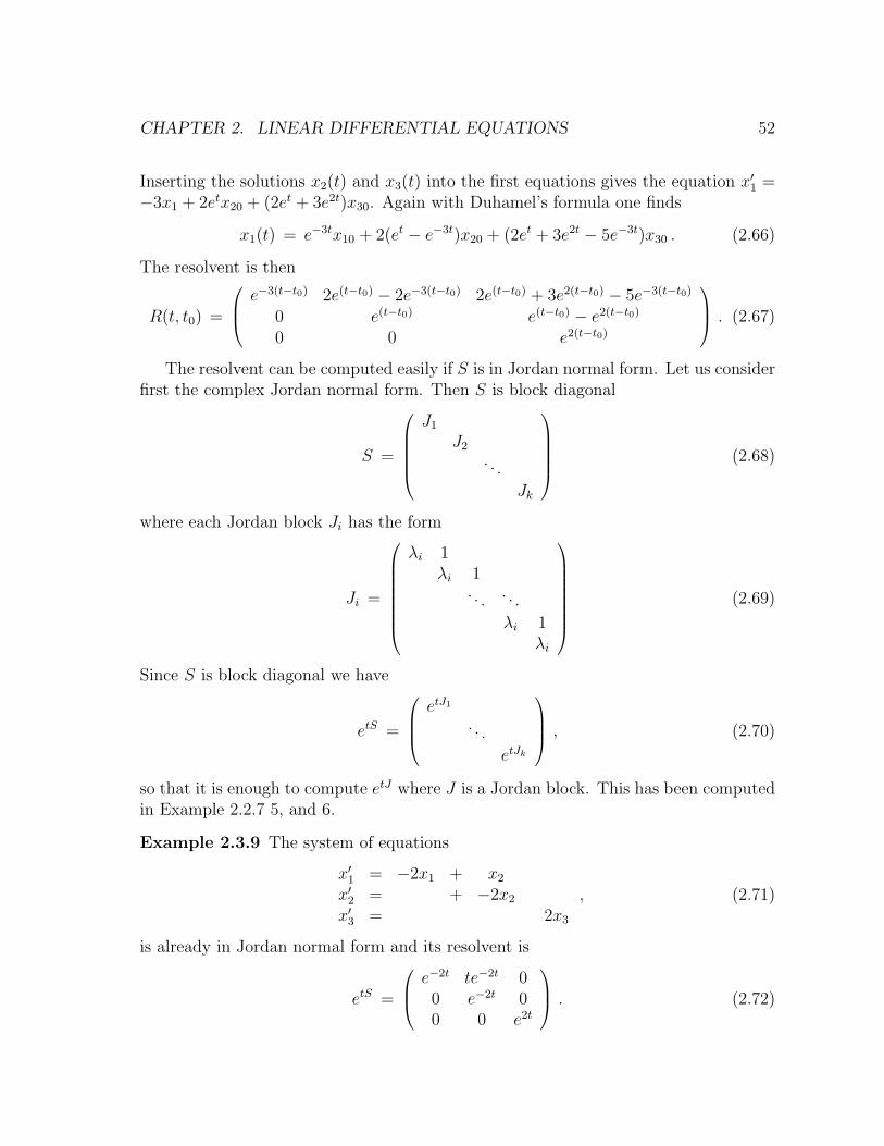
CHAPTER 2. LINEAR DIFFERENTIAL EQUATIONS 52
Inserting the solutions x2(t) and x3(t) into the first equations gives the equation x′1 =−3x1 + 2etx20 + (2et + 3e2t)x30. Again with Duhamel’s formula one finds
x1(t) = e−3tx10 + 2(et − e−3t)x20 + (2et + 3e2t − 5e−3t)x30 . (2.66)
The resolvent is then
R(t, t0) =
e−3(t−t0) 2e(t−t0) − 2e−3(t−t0) 2e(t−t0) + 3e2(t−t0) − 5e−3(t−t0)
0 e(t−t0) e(t−t0) − e2(t−t0)
0 0 e2(t−t0)
. (2.67)
The resolvent can be computed easily if S is in Jordan normal form. Let us considerfirst the complex Jordan normal form. Then S is block diagonal
S =
J1
J2
. . .
Jk
(2.68)
where each Jordan block Ji has the form
Ji =
λi 1λi 1
. . . . . .
λi 1λi
(2.69)
Since S is block diagonal we have
etS =
etJ1
. . .
etJk
, (2.70)
so that it is enough to compute etJ where J is a Jordan block. This has been computedin Example 2.2.7 5, and 6.
Example 2.3.9 The system of equations
x′1 = −2x1 + x2
x′2 = + −2x2
x′3 = 2x3
, (2.71)
is already in Jordan normal form and its resolvent is
etS =
e−2t te−2t 00 e−2t 00 0 e2t
. (2.72)
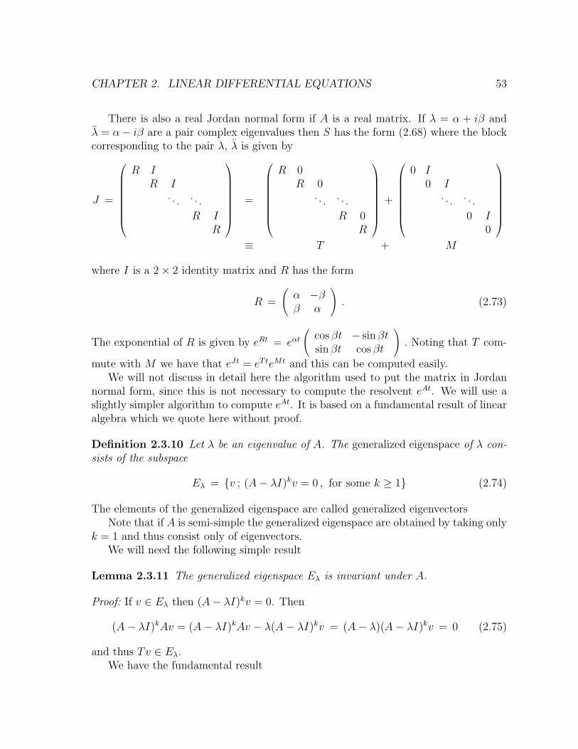
CHAPTER 2. LINEAR DIFFERENTIAL EQUATIONS 53
There is also a real Jordan normal form if A is a real matrix. If λ = α + iβ andλ = α− iβ are a pair complex eigenvalues then S has the form (2.68) where the blockcorresponding to the pair λ, λ is given by
J =
R IR I
. . . . . .
R IR
=
R 0R 0
. . . . . .
R 0R
+
0 I0 I
. . . . . .
0 I0
≡ T + M
where I is a 2× 2 identity matrix and R has the form
R =
(α −ββ α
). (2.73)
The exponential of R is given by eRt = eαt(
cos βt − sin βtsin βt cos βt
). Noting that T com-
mute with M we have that eJt = eTteMt and this can be computed easily.We will not discuss in detail here the algorithm used to put the matrix in Jordan
normal form, since this is not necessary to compute the resolvent eAt. We will use aslightly simpler algorithm to compute eAt. It is based on a fundamental result of linearalgebra which we quote here without proof.
Definition 2.3.10 Let λ be an eigenvalue of A. The generalized eigenspace of λ con-sists of the subspace
Eλ = {v ; (A− λI)kv = 0 , for some k ≥ 1} (2.74)
The elements of the generalized eigenspace are called generalized eigenvectorsNote that if A is semi-simple the generalized eigenspace are obtained by taking only
k = 1 and thus consist only of eigenvectors.We will need the following simple result
Lemma 2.3.11 The generalized eigenspace Eλ is invariant under A.
Proof: If v ∈ Eλ then (A− λI)kv = 0. Then
(A− λI)kAv = (A− λI)kAv − λ(A− λI)kv = (A− λ)(A− λI)kv = 0 (2.75)
and thus Tv ∈ Eλ.We have the fundamental result
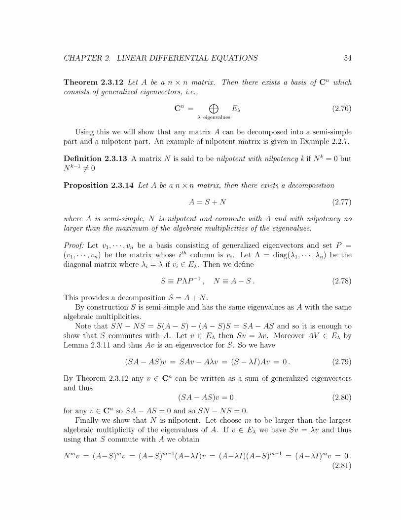
CHAPTER 2. LINEAR DIFFERENTIAL EQUATIONS 54
Theorem 2.3.12 Let A be a n × n matrix. Then there exists a basis of Cn whichconsists of generalized eigenvectors, i.e.,
Cn =⊕
λ eigenvalues
Eλ (2.76)
Using this we will show that any matrix A can be decomposed into a semi-simplepart and a nilpotent part. An example of nilpotent matrix is given in Example 2.2.7.
Definition 2.3.13 A matrix N is said to be nilpotent with nilpotency k if Nk = 0 butNk−1 6= 0
Proposition 2.3.14 Let A be a n× n matrix, then there exists a decomposition
A = S +N (2.77)
where A is semi-simple, N is nilpotent and commute with A and with nilpotency nolarger than the maximum of the algebraic multiplicities of the eigenvalues.
Proof: Let v1, · · · , vn be a basis consisting of generalized eigenvectors and set P =(v1, · · · , vn) be the matrix whose ith column is vi. Let Λ = diag(λ1, · · · , λn) be thediagonal matrix where λi = λ if vi ∈ Eλ. Then we define
S ≡ PΛP−1 , N ≡ A− S . (2.78)
This provides a decomposition S = A+N .By construction S is semi-simple and has the same eigenvalues as A with the same
algebraic multiplicities.Note that SN − NS = S(A − S) − (A − S)S = SA − AS and so it is enough to
show that S commutes with A. Let v ∈ EΛ then Sv = λv. Moreover AV ∈ Eλ byLemma 2.3.11 and thus Av is an eigenvector for S. So we have
(SA− AS)v = SAv − Aλv = (S − λI)Av = 0 . (2.79)
By Theorem 2.3.12 any v ∈ Cn can be written as a sum of generalized eigenvectorsand thus
(SA− AS)v = 0 . (2.80)
for any v ∈ Cn so SA− AS = 0 and so SN −NS = 0.Finally we show that N is nilpotent. Let choose m to be larger than the largest
algebraic multiplicity of the eigenvalues of A. If v ∈ Eλ we have Sv = λv and thususing that S commute with A we obtain
Nmv = (A−S)mv = (A−S)m−1(A−λI)v = (A−λI)(A−S)m−1 = (A−λI)mv = 0 .(2.81)
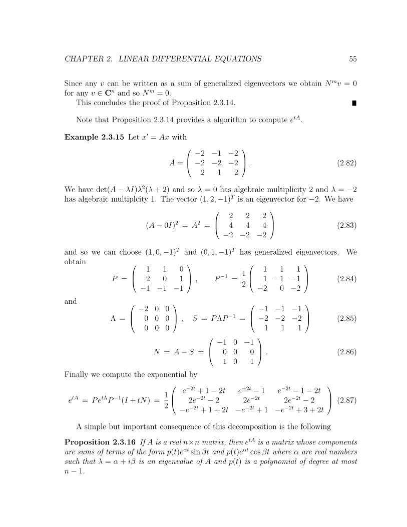
CHAPTER 2. LINEAR DIFFERENTIAL EQUATIONS 55
Since any v can be written as a sum of generalized eigenvectors we obtain Nmv = 0for any v ∈ Cn and so Nm = 0.
This concludes the proof of Proposition 2.3.14.
Note that Proposition 2.3.14 provides a algorithm to compute etA.
Example 2.3.15 Let x′ = Ax with
A =
−2 −1 −2−2 −2 −2
2 1 2
. (2.82)
We have det(A − λI)λ2(λ + 2) and so λ = 0 has algebraic multiplicity 2 and λ = −2has algebraic multiplcity 1. The vector (1, 2,−1)T is an eigenvector for −2. We have
(A− 0I)2 = A2 =
2 2 24 4 4−2 −2 −2
(2.83)
and so we can choose (1, 0,−1)T and (0, 1,−1)T has generalized eigenvectors. Weobtain
P =
1 1 02 0 1−1 −1 −1
, P−1 =1
2
1 1 11 −1 −1−2 0 −2
(2.84)
and
Λ =
−2 0 00 0 00 0 0
, S = PΛP−1 =
−1 −1 −1−2 −2 −2
1 1 1
(2.85)
N = A− S =
−1 0 −10 0 01 0 1
. (2.86)
Finally we compute the exponential by
etA = PetΛP−1(I + tN) =1
2
e−2t + 1− 2t e−2t − 1 e−2t − 1− 2t2e−2t − 2 2e−2t 2e−2t − 2
−e−2t + 1 + 2t −e−2t + 1 −e−2t + 3 + 2t
(2.87)
A simple but important consequence of this decomposition is the following
Proposition 2.3.16 If A is a real n×n matrix, then etA is a matrix whose componentsare sums of terms of the form p(t)eαt sin βt and p(t)eαt cos βt where α are real numberssuch that λ = α + iβ is an eigenvalue of A and p(t) is a polynomial of degree at mostn− 1.
CHAPTER 2. LINEAR DIFFERENTIAL EQUATIONS 56
2.4 Stability of linear systems
For the ODE, x′ = f(t, x) we say that x0 is a critical point if f(t, x0) = 0 for all t. Thisimplies that the constant solution x(t) = x0 is a solution of the Cauchy problem withx(t0) = x0. Critical points are also called equilibrium points.
For a linear system with constant coefficients, i.e., f(x) = Ax, x0 = 0 is alwayscritical point and it is the only critical point if det(A) 6= 0. If det(A) = 0, then 0 is aneigenvalue and any point in the eigenspace of the eigenvalue 0 is a critical point.
We define next the concept of stability of a solution
Definition 2.4.1 Let f : R × Rn → Rn be continuous and locally Lipschitz. Letx(t, t0, x) be the solution of the Cauchy problem x′ = f(t, x), x(t0) = x0 which weassume to exist for all times t > t0.
1. The solution x(t, t0, x0) is stable (in the sense of Liapunov) if for any ε > 0,there exists δ > 0 such that for all ξ with ‖ξ‖ ≤ δ we have
‖x(t, t0, x0 + ξ)− x(t, t0, x0)‖ ≤ ε for all t ≥ t0 . (2.88)
2. The solution x(t, t0, x0) is asymptotically stable if it is stable and there existsδ > 0 such that hat for all ξ with ‖ξ‖ ≤ δ we have
limt→∞‖x(t, t0, x0 + ξ)− x(t, t0, x0)‖ = 0 . (2.89)
3. The solution x(t, t0, x0) is unstable if it is not stable.
If a is a critical point, we will say the critical point a is stable or unstable if thesolution x(t) ≡ a is stable or unstable.
Example 2.4.2 The solution x(t) = 0 of x′ = λx is asymptotically stable of λ < 0,stable if λ = 0, unstable if λ > 0.
Example 2.4.3 The solutions of the equation x′′+ x = 0 are stable (but not asymp-totically stable). The general solution is (a cos(t) + b sin(t),−a sin(t) + b cos(t)) is aperiodic solution of period 2π on the circle of radius a2 + b2. Two solutions starting atnearby points (x1, y1) and (x0, y0) will remain close forever.
Example 2.4.4 The solution x(t, 0, x0) = x0
1−x0tof x′ = x2 is asymptotically stable for
x0 < 0 but unstable for x0 ≥ 0.
Example 2.4.5 For the ODE x′ = x2 − 1, there are two critical points 0 and 1. Thesolution x(t) = 0 is unstable and the solution x(t) = 1 is stable.
CHAPTER 2. LINEAR DIFFERENTIAL EQUATIONS 57
For a linear homogeneous equation x′ = A(t)x we have x(t, t0, x0 +ξ)−x(t, t0, x0) =R(t, t0)ξ = x(t, t0, ξ) − x(t, t0, 0) and so it suffices to study the stability of the crit-ical point 0. For a linear inhomogeneous equation x′ = A(t)x + f(t), the differencex(t, t0, x0 + ξ)− x(t, t0, x0) is again equal to R(t, t0)ξ where R(t, t0) is the resolvent ofthe homogeneous equation x′ = A(t)x and thus the stability properties of a solutionx(t) of the inhomogeneous problem are the same as the stability of the trivial solutionof the homogeneous problem. Therefore, in the case of linear differential equations, allthe solutions have the same stability properties and one can talk about the stability ofthe differential equation.
As we have seen in Section 2.3, the solutions of linear systems with constant co-efficients are determined by the eigenvalues, and the generalized eigenvectors of thematrix A. We define the stable, unstable and center subspaces, denoted respectively byEs, Eu, and Ec and defined by
Es =⊕
λ : Reλ<0
Ei , (2.90)
Eu =⊕
λ : Reλ>0
Ei , (2.91)
Ec =⊕
λ : Reλ=0
Ei . (2.92)
(2.93)
By Lemma 2.3.11 amd Theorem 2.3.12 the generalized eigenspaces span the wholespace and are invariant under A and thus also under etA. So we have
Rn = Es ⊕ Eu ⊕ Ec , (2.94)
andeAtE# = E# , for all t ∈ R , # = s, u, c . (2.95)
From the proposition 2.3.16 we obtain
Theorem 2.4.6 Let x′ = Ax be a linear system with constant coefficients x′ = Ax,and let λ1, · · · , λk be the eigenvalues of A.(a) The critical point 0 is asymptotically stable if and only if all the eigenvalues of Ahave a negative real part: Reλi < 0 for i = 1, · · · , k, i.e., if Es = Rn.(b) The critical point 0 is stable if and only
1. All the eigenvalues have a nonpositive real part Reλi ≤ 0 for i = 1, · · · , k, i.e.,Es ⊕ Ec = Rn.
2. If Reλi = 0 the Jordan blocks have dimension 1.
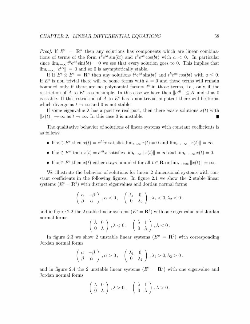
CHAPTER 2. LINEAR DIFFERENTIAL EQUATIONS 58
Proof: If Es = Rn then any solutions has components which are linear combina-tions of terms of the form tkeαt sin(bt) and tkeαt cos(bt) with a < 0. In particularsince limt→∞ t
keαt sin(bt) = 0 we see that every solution goes to 0. This implies thatlimt→∞ ‖etA‖ = 0 and so 0 is asymptotically stable.
If If Es ⊗ Ec = Rn then any solutions tkeαt sin(bt) and tkeαt cos(bt) with a ≤ 0.If Ec is non trivial there will be some terms with a = 0 and those terms will remainbounded only if there are no polynomial factors tk,in those terms, i.e., only if therestriction of A to Ec is semisimple. In this case we have then ‖eAt‖ ≤ K and thus 0is stable. If the restriction of A to Ec has a non-trivial nilpotent there will be termswhich diverge as t→∞ and 0 is not stable.
If some eigenvalue λ has a positive real part, then there exists solutions x(t) with‖x(t)‖ → ∞ as t→∞. In this case 0 is unstable.
The qualitative behavior of solutions of linear systems with constant coefficients isas follows
• If x ∈ Es then x(t) = eAtx satisfies limt→∞ x(t) = 0 and limt→−∞ ‖x(t)‖ =∞.
• If x ∈ Eu then x(t) = eAtx satisfies limt→∞ ‖x(t)‖ =∞ and limt→−∞ x(t) = 0.
• If x ∈ Ec then x(t) either stays bounded for all t ∈ R or limt→±∞ ‖x(t)‖ =∞.
We illustrate the behavior of solutions for linear 2 dimensional systems with con-stant coefficients in the following figures. In figure 2.1 we show the 2 stable linearsystems (Es = R2) with distinct eigenvalues and Jordan normal forms(
α −ββ α
), α < 0 ,
(λ1 00 λ2
), λ1 < 0, λ2 < 0 .
and in figure 2.2 the 2 stable linear systems (Es = R2) with one eigenvalue and Jordannormal forms (
λ 00 λ
), λ < 0 ,
(λ 10 λ
), λ < 0 .
In figure 2.3 we show 2 unstable linear systems (Eu = R2) with correspondingJordan normal forms(
α −ββ α
), α > 0 ,
(λ1 00 λ2
), λ1 > 0, λ2 > 0 .
and in figure 2.4 the 2 unstable linear systems (Es = R2) with one eigenvalue andJordan normal forms (
λ 00 λ
), λ > 0 ,
(λ 10 λ
), λ > 0 .
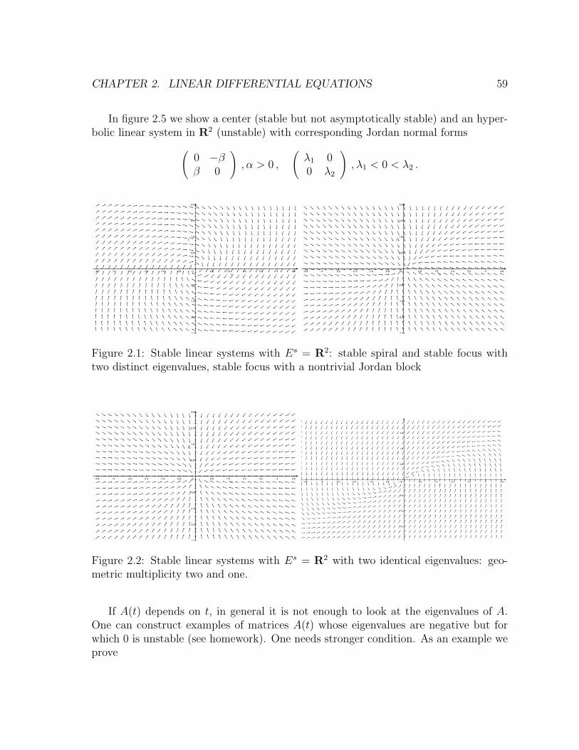
CHAPTER 2. LINEAR DIFFERENTIAL EQUATIONS 59
In figure 2.5 we show a center (stable but not asymptotically stable) and an hyper-bolic linear system in R2 (unstable) with corresponding Jordan normal forms(
0 −ββ 0
), α > 0 ,
(λ1 00 λ2
), λ1 < 0 < λ2 .
-4.8 -4 -3.2 -2.4 -1.6 -0.8 0 0.8 1.6 2.4 3.2 4 4.8
-3.2
-2.4
-1.6
-0.8
0.8
1.6
2.4
3.2
-4.8 -4 -3.2 -2.4 -1.6 -0.8 0 0.8 1.6 2.4 3.2 4 4.8
-3.2
-2.4
-1.6
-0.8
0.8
1.6
2.4
3.2
Figure 2.1: Stable linear systems with Es = R2: stable spiral and stable focus withtwo distinct eigenvalues, stable focus with a nontrivial Jordan block
-4.8 -4 -3.2 -2.4 -1.6 -0.8 0 0.8 1.6 2.4 3.2 4 4.8
-3.2
-2.4
-1.6
-0.8
0.8
1.6
2.4
3.2
-4.8 -4 -3.2 -2.4 -1.6 -0.8 0 0.8 1.6 2.4 3.2 4 4.8
-2.4
-1.6
-0.8
0.8
1.6
2.4
Figure 2.2: Stable linear systems with Es = R2 with two identical eigenvalues: geo-metric multiplicity two and one.
If A(t) depends on t, in general it is not enough to look at the eigenvalues of A.One can construct examples of matrices A(t) whose eigenvalues are negative but forwhich 0 is unstable (see homework). One needs stronger condition. As an example weprove
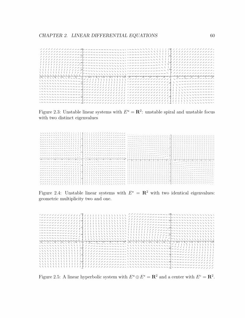
CHAPTER 2. LINEAR DIFFERENTIAL EQUATIONS 60
-4.8 -4 -3.2 -2.4 -1.6 -0.8 0 0.8 1.6 2.4 3.2 4 4.8
-3.2
-2.4
-1.6
-0.8
0.8
1.6
2.4
3.2
-4.8 -4 -3.2 -2.4 -1.6 -0.8 0 0.8 1.6 2.4 3.2 4 4.8
-3.2
-2.4
-1.6
-0.8
0.8
1.6
2.4
3.2
Figure 2.3: Unstable linear systems with Eu = R2: unstable spiral and unstable focuswith two distinct eigenvalues
-4.8 -4 -3.2 -2.4 -1.6 -0.8 0 0.8 1.6 2.4 3.2 4 4.8
-2.4
-1.6
-0.8
0.8
1.6
2.4
-5 -4.5 -4 -3.5 -3 -2.5 -2 -1.5 -1 -0.5 0 0.5 1 1.5 2 2.5 3 3.5 4 4.5 5
-2.5
-2
-1.5
-1
-0.5
0.5
1
1.5
2
2.5
Figure 2.4: Unstable linear systems with Es = R2 with two identical eigenvalues:geometric multiplicity two and one.
-4.8 -4 -3.2 -2.4 -1.6 -0.8 0 0.8 1.6 2.4 3.2 4 4.8
-3.2
-2.4
-1.6
-0.8
0.8
1.6
2.4
3.2
-4.8 -4 -3.2 -2.4 -1.6 -0.8 0 0.8 1.6 2.4 3.2 4 4.8
-3.2
-2.4
-1.6
-0.8
0.8
1.6
2.4
3.2
Figure 2.5: A linear hyperbolic system with Eu⊕Es = R2 and a center with Ec = R2.
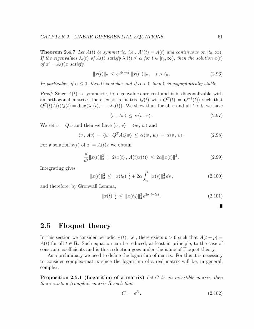
CHAPTER 2. LINEAR DIFFERENTIAL EQUATIONS 61
Theorem 2.4.7 Let A(t) be symmetric, i.e., A∗(t) = A(t) and continuous on [t0,∞).If the eigenvalues λi(t) of A(t) satisfy λi(t) ≤ α for t ∈ [t0,∞), then the solution x(t)of x′ = A(t)x satisfy
‖x(t)‖2 ≤ eα(t−t0)‖x(t0)‖2 , t > t0 . (2.96)
In particular, if α ≤ 0, then 0 is stable and if α < 0 then 0 is asymptotically stable.
Proof: Since A(t) is symmetric, its eigenvalues are real and it is diagonalizable withan orthogonal matrix: there exists a matrix Q(t) with QT (t) = Q−1(t)) such thatQT (t)A(t)Q(t) = diag(λ1(t), · · · , λn(t)). We show that, for all v and all t > t0 we have
〈v , Av〉 ≤ α〈v , v〉 . (2.97)
We set v = Qw and then we have 〈v , v〉 = 〈w , w〉 and
〈v , Av〉 = 〈w , QTAQw〉 ≤ α〈w , w〉 = α〈v , v〉 . (2.98)
For a solution x(t) of x′ = A(t)x we obtain
d
dt‖x(t)‖2
2 = 2〈x(t) , A(t)x(t)〉 ≤ 2α‖x(t)‖2 . (2.99)
Integrating gives
‖x(t)‖22 ≤ ‖x(t0)‖2
2 + 2α∫ t
t0‖x(s)‖2
2 ds , (2.100)
and therefore, by Gronwall Lemma,
‖x(t)‖22 ≤ ‖x(t0)‖2
2 e2α(t−t0) . (2.101)
2.5 Floquet theory
In this section we consider periodic A(t), i.e., there exists p > 0 such that A(t + p) =A(t) for all t ∈ R. Such equation can be reduced, at least in principle, to the case ofconstants coefficients and is this reduction goes under the name of Floquet theory.
As a preliminary we need to define the logarithm of matrix. For this it is necessaryto consider complex-matrix since the logarithm of a real matrix will be, in general,complex.
Proposition 2.5.1 (Logarithm of a matrix) Let C be an invertible matrix, thenthere exists a (complex) matrix R such that
C = eR . (2.102)
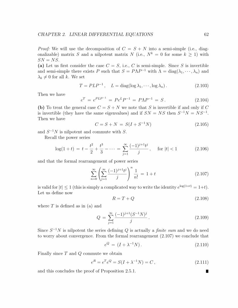
CHAPTER 2. LINEAR DIFFERENTIAL EQUATIONS 62
Proof: We will use the decomposition of C = S + N into a semi-simple (i.e., diag-onalizable) matrix S and a nilpotent matrix N (i.e., Nk = 0 for some k ≥ 1) withSN = NS.(a) Let us first consider the case C = S, i.e., C is semi-simple. Since S is invertibleand semi-simple there exists P such that S = PΛP−1 with Λ = diag(λ1, · · · , λn) andλk 6= 0 for all k. We set
T = PLP−1 , L = diag(log λ1, · · · , log λn) . (2.103)
Then we haveeT = ePLP
−1
= PeLP−1 = PΛP−1 = S . (2.104)
(b) To treat the general case C = S +N we note that S is invertible if and only if Cis invertible (they have the same eigenvalues) and if SN = NS then S−1N = NS−1.Then we have
C = S +N = S(I + S−1N) (2.105)
and S−1N is nilpotent and commute with S.Recall the power series
log(1 + t) = t− t2
2+t3
3− · · · =
∞∑j=1
(−1)j+1tj
j, for |t| < 1 (2.106)
and that the formal rearrangement of power series
∞∑n=0
∞∑j=1
(−1)j+1tj
j
n 1
n!= 1 + t (2.107)
is valid for |t| ≤ 1 (this is simply a complicated way to write the identity elog(1+t) = 1+t).Let us define now
R = T +Q (2.108)
where T is defined as in (a) and
Q =∞∑j=1
(−1)j+1(S−1N)j
j. (2.109)
Since S−1N is nilpotent the series defining Q is actually a finite sum and we do needto worry about convergence. From the formal rearrangement (2.107) we conclude that
eQ = (I + λ−1N) . (2.110)
Finally since T and Q commute we obtain
eR = eT eQ = S(I + λ−1N) = C , (2.111)
and this concludes the proof of Proposition 2.5.1.
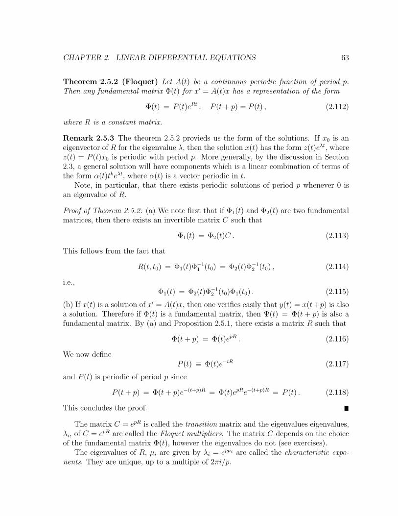
CHAPTER 2. LINEAR DIFFERENTIAL EQUATIONS 63
Theorem 2.5.2 (Floquet) Let A(t) be a continuous periodic function of period p.Then any fundamental matrix Φ(t) for x′ = A(t)x has a representation of the form
Φ(t) = P (t)eRt , P (t+ p) = P (t) , (2.112)
where R is a constant matrix.
Remark 2.5.3 The theorem 2.5.2 provieds us the form of the solutions. If x0 is aneigenvector of R for the eigenvalue λ, then the solution x(t) has the form z(t)eλt, wherez(t) = P (t)x0 is periodic with period p. More generally, by the discussion in Section2.3, a general solution will have components which is a linear combination of terms ofthe form α(t)tkeλt, where α(t) is a vector periodic in t.
Note, in particular, that there exists periodic solutions of period p whenever 0 isan eigenvalue of R.
Proof of Theorem 2.5.2: (a) We note first that if Φ1(t) and Φ2(t) are two fundamentalmatrices, then there exists an invertible matrix C such that
Φ1(t) = Φ2(t)C . (2.113)
This follows from the fact that
R(t, t0) = Φ1(t)Φ−11 (t0) = Φ2(t)Φ−1
2 (t0) , (2.114)
i.e.,Φ1(t) = Φ2(t)Φ−1
2 (t0)Φ1(t0) . (2.115)
(b) If x(t) is a solution of x′ = A(t)x, then one verifies easily that y(t) = x(t+p) is alsoa solution. Therefore if Φ(t) is a fundamental matrix, then Ψ(t) = Φ(t + p) is also afundamental matrix. By (a) and Proposition 2.5.1, there exists a matrix R such that
Φ(t+ p) = Φ(t)epR . (2.116)
We now defineP (t) ≡ Φ(t)e−tR (2.117)
and P (t) is periodic of period p since
P (t+ p) = Φ(t+ p)e−(t+p)R = Φ(t)epRe−(t+p)R = P (t) . (2.118)
This concludes the proof.
The matrix C = epR is called the transition matrix and the eigenvalues eigenvalues,λi, of C = epR are called the Floquet multipliers. The matrix C depends on the choiceof the fundamental matrix Φ(t), however the eigenvalues do not (see exercises).
The eigenvalues of R, µi are given by λi = epµi are called the characteristic expo-nents. They are unique, up to a multiple of 2πi/p.
CHAPTER 2. LINEAR DIFFERENTIAL EQUATIONS 64
Remark 2.5.4 For the equation x′ = A(t)x, let us consider the transformation
x(t) = P (t)y(t) (2.119)
where P (t) is the periodic matrix given by Floquet theorem. We obtain
x′(t) = P ′(t)y(t) + P (t)y′(t) = A(t)P (t)y(t) . (2.120)
On the other hand P (t) = Φ(t)e−Rt, so that
P ′(t) = Φ′(t)e−Rt − Φ(t)e−RtR = A(t)P (t)− P (t)R . (2.121)
Thus we findy′(t) = Ry(t) . (2.122)
The transformation x = P (t)y reduces the linear equation with periodic coefficientsx′ = A(t)x to the system with constant coefficients y′ = By. Nevertheless there are,in general, no methods available to compute P (t) or the Floquet multipliers. Eachequation has to be studied for itself and entire books are devoted to quite simplelooking equations. The Floquet theory is however very useful to study the stability ofperiodic solutions, as we shall see later.
Example 2.5.5 Let us consider the equation x′′+b(t)x′+a(t) = 0, where a(t) and b(t)are periodic functions. For the fundamental solution Φ(t) = R(t, 0) we have Φ(0) = Iand so by Floquet Theorem
Φ(p) = C = epR =
(x1(p) x2(p)x′1(p) x′2(p)
)(2.123)
The Floquet multipliers are given by the solutions of
λ2 + αλ+ β = 0 , (2.124)
where
α = −x1(p)−x′2(p) , β = det(C) = det(R(p, 0)) = e∫ p0
trA(s) ds = e−∫ p0b(s) ds (2.125)
In the special case where b(s) ≡ 0, then the equation is λ2 + αλ + 1 = 0. We havethen(i) If −2 < α < 2 then the Floquet multipliers λ and λ are complex conjugate withmodulus 1 and therefore the solutions are bounded for all t > 0.(ii) If α > 2 or α < −2, at least one eigenvalue of C has modulus greater than 1 andthere exists solutions such that |x(t)|2 + |x′(t)|2 goes to infinity as t goes to infinity.(iii) If α = −2, then λ = 1 is the eigenvalue of C and therefore there exists a periodicsolution of period p. If α = 2 then λ = −1 is the eigenvalue of C and therefore thereexists a periodic solution of period 2p.
CHAPTER 2. LINEAR DIFFERENTIAL EQUATIONS 65
2.6 Linearization
Let us consider the solution x(t, t0, x0) of the Cauchy problem x′ = f(t, x), x(t0) = x0.Let ξ ∈ Rn and let us now consider the solution x(t, t0, x0 + ξ). As we have seen inSection 1.7 the function ξ 7→ x(t, t0, x0 + ξ) is continuous, in fact Lipschitz continuous,provided f is continuous and satisfy a Lipschitz condition. If we assume f to be ofclass C1, it is natural to ask whether the map ξ 7→ x(t, t0, x0 + ξ) is of class C1? If thisis the case we have the Taylor expansion
x(t, t0, x0 + ξ) = x(t, t0, x0) +∂x
∂x0
(t, t0, x0)ξ + o(‖ξ‖) , (2.126)
where o(‖ξ‖) stands for a function with lim‖ξ‖→0 o(‖ξ‖)/‖ξ‖ = 0. The right handside of (2.126) without the o(‖ξ‖) term is called the linearization around the solutionx(t, t0, x0).
To obtain an idea of the form of the derivative ∂x∂x0
(t, t0, x0) we write the Cauchyproblem as
∂x
∂t(t, t0, x0) = f(t, x(t, t0, x0)) , x(t0, t0, x0) = x0 , (2.127)
and differentiate formally with respect to x0. Exchanging the derivatives with respectto t and x0 we find
∂
∂t
∂x
∂x0
(t, t0, x0) =∂f
∂x(t, x(t, t0, x0))
∂x
∂x0
(t, t0, x0) ,∂x
∂x0
(t0, t0, x0) = I . (2.128)
This formal calculation shows that the n × n matrix ∂x∂x0
(t, t0, x0) is a solution of thelinear equation
Ψ′ =∂f
∂x(t, x(t, t0, x0))Ψ , Ψ(t0) = I . (2.129)
This equation is called the variational equation for the Cauchy problem x′ = f(t, x),x(t0) = x0. It is a linear equation of the form y′ = A(t; t0, x0)y, where the matrix Adepends on the parameters (t0, x0). The resolvent also depends on this parameters andlet us denote it by R(t, s; t0, x0). The formal calculation shows that
∂x
∂x0
(t, t0, x0) = R(t, t0; t0, x0) . (2.130)
Before we prove that this formal computation is actually correct let us consider anumber of important special cases and example
Example 2.6.1 (Linearization around equilibrium solutions)Let us assume thatthe ODE is autonomous, f(t, x) = f(x) with f of class C1 and that a is a critical point,
CHAPTER 2. LINEAR DIFFERENTIAL EQUATIONS 66
i.e., f(a) = 0. The constant solution x(t, 0, a) = a is a solution. The variationalequation is then
Ψ′ =df
dx(a)Ψ , Ψ(0) = I , (2.131)
whose solution is etA where A = dfdx
(a). Therefore, for small ξ, we have
x(t, 0, a+ ξ) = a+ etAξ + o(‖ξ‖) . (2.132)
Example 2.6.2 Consider the mathematical pendulum x′′ + sin(x) = 0 or
x′ = y ,
y′ = − sin(x) . (2.133)
There are two equilibrium solution a = (π, 0)T and b = (0, 0)T (the first componentmodulo 2π). The linearization around a and b gives, for small ξ,
z(t, 0, (π, 0)T + ξ) ≈(π0
)+ eAtξ , A =
(0 11 0
), (2.134)
where A has eigenvalues ±1 and
z(t, 0, ξ) ≈(
00
)+ eBtξ , B =
(0 1−1 0
)(2.135)
where B has eigenvalues ±i.
Example 2.6.3 (Linearization around a periodic solution) Let us assume thatthe nonlinear equation x′ = f(x) has a periodic solution x(t, 0, x0) = φ(t). If welinearize around this periodic solution the variational equation is given by
x′ =df
dx(φ(t))x . (2.136)
which is a linear equation with periodic coefficients that we can analyze using Floquettheory of Section 2.5.
An important fact is the following. If φ(t) is aperiodic solution then φ′(t) is asolution of the variational equation (2.136). Indeed we have
φ′′(t) =d
dtf(φ(t)) =
df
dx(φ(t))φ′(t) . (2.137)
In particular, in two dimensions, if φ(t) is known explicitly, this can be used to solvethe variational equation, using D’Alembert reduction method (see exercises).
CHAPTER 2. LINEAR DIFFERENTIAL EQUATIONS 67
Example 2.6.4 The second order equation x′′+f(x)x′+ g(x) = 0 has, under suitableconditions (see Chapter 4) a periodic solution φ(t). In this case the variational equationis given by
x′ = y ,
y′ = − (f(φ(t))φ′(t) + g′(φ(t)))x− f(φ(t))y . (2.138)
and has the form x′′ + b(t)x′ + a(t) = 0, where a(t) and b(t) are periodic functions.
Example 2.6.5 The system
x′ = −y + x(1− x2 − y2) , (2.139)
y′ = x+ y(1− x2 − y2) , (2.140)
z′ = z . (2.141)
has a periodic orbit in the x, y plane given by (cos(t), sin(t), 0)T . This can be verifiedby direct computation or be deduced by choosing cylindrical coordinates (r, θ, z) andshowing that the system (2.185) is equivalent to
r′ = r(1− r2) , (2.142)
θ′ = 1, (2.143)
z′ = z . (2.144)
The linearization around the periodic orbit gives the variational equation
Ψ′ =
−2 cos2(t) −1− 2 cos(t) sin(t) 01− 2 cos(t) sin(t) −2 sin2(t) 0
0 0 1
Ψ (2.145)
Using the fact that φ′(t) = (− sin(t), cos(t), 0) is a solution, one can compute thesolution of the variational equation (see exercises).
Theorem 2.6.6 Let U ⊂ R×Rn be an open set, f : U → Rn be continuous. Assumethat ∂f
∂x(t, x) exists and is continuous on U . Then the solution x(t, t0, x0) of x′ = f(x),
x(t0) = x0 is continuously differentiable with respect to x0 and its derivative ∂x∂x0
(t, t0, x0)is a solution of the variational equation
Ψ′ =∂f
∂x(t, x(t, t0, x0))Ψ , Ψ(t0) = I . (2.146)
Proof: For given (t, t0, x0) let us choose [a, b] ⊂ Imax such that t, t0 ∈ (a, b). Let ξ ∈ Rn,we need to show that for fixed (t, t0, x0),
x(t, t0, x0 + ξ)− x(t, t0, x0)−R(t, t0; t0, x0)ξ = o(‖ξ‖) , (2.147)
CHAPTER 2. LINEAR DIFFERENTIAL EQUATIONS 68
where o(‖ξ‖)/‖ξ‖ → 0 as ξ → 0. The integral equations for x(t, t0, x0 + ξ), x(t, t0, x0)and R(t, t0; t0, x0)ξ are respectively
x(t, t0, x0 + ξ) = x0 + ξ +∫ t
t0f(s, x(s, t0, x0 + ξ)) ds
x(t, t0, x0) = x0 +∫ t
t0f(s, x(s, t0, x0)) ds
R(t, t0; t0, x0)ξ = ξ +∫ t
t0
∂f
∂x(s, x(s, t0, x0))R(s, t0; t0, x0)ξ ds (2.148)
By Theorem 1.7.3, there exists a constant D such that ‖x(s, t0, x0 + ξ)−x(s, t0, x0)‖ ≤D‖ξ‖ for t0 ≤ s ≤ t provided ‖ξ‖ is small enough and thus we have
o(‖x(s, t0, x0 + ξ)− x(s, t0, x0)‖) = o(‖ξ‖) . (2.149)
We use the Taylor approximation
f(s, z)− f(s, y)− ∂f
∂x(s, y)(z − y) = o(‖z − y‖) , (2.150)
and we can take the right hand side to be uniform in (s, y) in any compact set Ksince f is of class C1 and will apply it to z = x(s, t0, x0 + ξ) and y = x(s, t0, x0) witht0 ≤ s ≤ t.
Using these estimates with the integral equations we obtain that
‖x(t, t0, x0 + ξ)− x(t, t0, x0)−R(t, t0; t0, x0)ξ‖
≤∫ t
t0
∂f
∂x(s, x(s, t0, x0))(x(s, t0, x0 + ξ)− x(s, t0, x0)−R(s, t0; t0, x0)ξ) ds
+∫ t
t0o(‖x(s, t0, x0 + ξ)− x(s, t0, x0)‖) ds .
≤ C∫ t
t0‖x(s, t0, x0 + ξ)− x(s, t0, x0)−R(s, t0; t0, x0)ξ‖ ds+ (b− a)o(‖ξ‖) ,
where C = sups∈[a,b]
{∥∥∥∂f∂x
(s, x(s, t0, x0))∥∥∥}. By Gronwall Lemma we conclude that
‖x(t, t0, x0+ξ)−x(t, t0, x0)−R(t, t0; t0, x0)ξ‖ ≤ (b−a)eC(b−a)o(‖ξ‖) = o(‖ξ‖) , (2.151)
and this shows that the derivative exists and satisfies the variational equation. It re-mains to show that the derivative ∂x
∂x0(t, t0, x0) is a continuous function. We cannot
apply Theorem 1.7.3 directly, since (t0, x0) are not the initial conditions for the varia-tional equation, but are parameters of the equation. We will show this in Lemma 2.6.7.
CHAPTER 2. LINEAR DIFFERENTIAL EQUATIONS 69
Lemma 2.6.7 Let I is an open interval and V an open set in Rq. Assume that A(t; c)is continuous on I × V . Then the resolvent R(t, t0; c) for the differential equationx′ = A(t; c)x is a continuous function of c.
Proof: The proof is a special case of the continuous dependence of solutions on param-eters (see exercises).
Note that if the ODE is autonomous we obtain
Corollary 2.6.8 Let f : Rn → Rn be of class C1 and let us assume that the solutionsof x′ = f(x) exist for all time. Then, for any t, the maps φt : Rn → Rn are of classC1 and so φt defines a C1 dynamical system, i.e. a group of diffeomorphisms.
We discuss next the smooth dependence with respect to parameters and with re-spect to t0. Let us consider a Cauchy problem x′ = f(t, x, c) where f : U → Rn isdifferentiable with respect to x and c (U is an open set of R×Rn×Rq). The solutionis denoted x(t, t0, x0, c)
In order to study the differentiability with respect to the parameters c we considerthe extended system(
xc
)′=
(f(t, x, c)
0
),
(xc
)(t0) =
(x0
c
)(2.152)
If we set z = (x, c)T and F (t, z) = (f(t, x, c), 0)T , then this system becomes z′ = F (t, z),z(0) = (x0, c)
T and c appears only in the initial condition. Therefore we can applyTheorem 2.6.6. The function z(t, t0, z0) is continuously differentiable with respect toz0 = (x0, c) and therefore x(t, t0, x0, c) is continuously differentiable with respect to c.By deriving the equation
∂x
∂t(t, t0, x0, c) = f(t, x(t, t0, x0, c), c) , x(t0, t0, x0, c) = x0 (2.153)
with respect to c we find a linear inhomogeneous equation for Ψ(t) = ∂x∂c
(t, t0, x0, c):
Ψ′ =∂f
∂x(t, x(t, t0, x0, c), c)Ψ +
∂f
∂c(t, x(t, t0, x0, c), c) , Ψ(0) = 0 . (2.154)
Example 2.6.9 The solution of the problem
x′ = f(t, x) + εg(t, x) , x(t0) = x0 . (2.155)
is given, for small |ε| by x(t, ε) = x0(t) + εx1(t) + o(ε) where
x′0(t) = f(t, x0(t)) , x(t) = x0 ,
x′1(t) =∂f
∂x(t, x0(t))x1(t) + g(t, x0(t)) , x1(t) = 0 . (2.156)
If we solve the first equation and find x0(t), the second equation is a linear inhomoge-neous equation for x1(t)
CHAPTER 2. LINEAR DIFFERENTIAL EQUATIONS 70
Example 2.6.10 Consider the equation x′ + x − εx3 with x(0) = 1. For ε = 0the solution is x0(t) = e−t. Expanding around this solution we find that x(t) =x0(t) + εx1(t) + o(ε) where x1(t) is a solution of
x′1 = −x1 + e−3t , x1(0) = 0 (2.157)
so that x(t) = e−t + ε(e−t − 12e−3t) + o(ε).
Let us assume that f(t, x) is continuously differentiable with respect to t and x.Let us consider the extended system(
xt
)′=
(f(t, x)
1
),
(xt
)(t0) =
(x0
t0
)(2.158)
If we set z = (x, t)T and F (z) = (f(t, x), 1)T , then this system becomes z′ = F (z),z(t0) = (x0, t0)T and the dependence on t0 can be studied as the dependence on x0.By Theorem 2.6.6, the solution x(t, t0, x0) is continuously differentiable with respect tot0. Differentiating the equation ∂x
∂t(t, t0, x0) = f(t, x(t, t0, x0)) with x(t0, t0, x0, ) = x0
with respect to t0, one finds a linear equation for Ψ(t) = ∂x0
∂t(t, t0, x0)
Ψ′ =∂f
∂x(t, x(t, t0, x0))Ψ , Ψ(t0) = −f(t0, x0) . (2.159)
This is the same differential equation as in the variational equation for ∂x∂x0
(t, t0, x0)
but with a different initial condition. Since ∂x∂x0
(t, t0, x0) is the resolvent of (2.159) weobtain the relation
∂x
∂t0(t, t0, x0) = − ∂x
∂x0
(t, t0, x0)f(t0, x0) . (2.160)
We can summarize the result of this section by
Theorem 2.6.11 Let U ⊂ R×Rn be an open set and let f : U → Rn be of class Ck,then the solution x(t, t0, x0) is of class Ck in the variables (t, t0, x0).
Proof: We have proved that x(t, t0, x0) is differentiable with respect to x0 and t0. Thedifferentiability with respect to t is automatic. We can apply this argument iterativelyto the variational equation and see by recurrence that x is of class Ck.
2.7 Exercises
1. If A ∈ L(Kn) the spectral radius of A, ρ(A), is defined by
ρ(A) = max{|λ| ; λ eigenvalue of A} . (2.161)
CHAPTER 2. LINEAR DIFFERENTIAL EQUATIONS 71
(a) Let
A =
(0.999 1000
0 0.999
)(2.162)
Compute the spectral radius of A as well as ‖A‖1, ‖A‖2, and ‖A‖∞. Find anorm on Rn such that ‖A‖ ≤ 1.
(b) Show that for any norm on Kn we have the inequality ρ(A) ≤ ‖A‖.(c) Show that if A is symmetric (A∗ = A) then we have the equality ‖A‖2 =
ρ(A).
(d) Show that for any A and any ε > 0, there exists a norm such that ‖A‖ ≤ρ(A) + ε. Hint: You may use (without proof) the fact that there exists amatrix D such that DAD−1 is upper triangular (or maybe even in Jordannormal form). Consider the diagonal matrix S with entries 1, µ−1, · · · , µ1−n.Set ‖x‖µ = ‖SDx‖ where ‖ · ‖ is any norm on Rn.
2. We have shown in class, using the binomial theorem, that if the matrices A and Bcommute then eA+B = eAeB. Here you will show, using a different method basedon uniqueness of solutions for ODE that eA+B = eAeB if and only if AB = BA.
(a) Let F (t) = BetA and G(t) = etAB. Show that if A and B commute thenF (t) and G(t) satisfies the same ODE and thus must be equal.
(b) Let Φ(t) = etAetB and Ψ(t) = et(A+B). Show that if A and B commute, thenΦ(t) and Ψ(t) satisfies the same ODE and thus must be equal.
(c) Show that if Φ(t) = Ψ(t) then A and B commute.
3. Show that if A(t) is antisymmetric, i.e., AT = −A, then the resolvant of x′ =A(t)x is orthogonal. Hint: Show that the scalar product of two solutions isconstant.
4. (D’Alembert reduction method). Consider the ODE x′ = A(t)x where A(t)is a n× n matrix and assume that we know one non-trivial solution x(t). Showthat one can reduce the equation x′ = A(t)x to the problem z′ = B(t)z wherez ∈ Rn−1 and B(t) is a (n−1)× (n−1) matrix. Hint: Without loss of generalityyou may assume that the nth component of x(t), xn(t) 6= 0. Look for solutionsof the form y(t) = φ(t)x(t) + z(t), where φ(t) is a scalar function and z has theform z = (z1, · · · , zn−1, 0)T .
5. (a) Using the previous problem, compute the resolvent R(t, 1) of
x′ =
(1t−1
1t2
2t
)x , (2.163)
CHAPTER 2. LINEAR DIFFERENTIAL EQUATIONS 72
using the fact that x(t) = (t2,−t)T is a solution. Hint: The solution is(t2(1− log t) −t2 log t
t log t t(1 + log t)
)(2.164)
(b) Compute the solution of
x′ =
(1t−1
1t2
2t
)x+
(t−t2
), (2.165)
with initial condition x(1) = (0, 0)T .
6. Compute the resolvant eAt for the equations x′ = Ax with
(a)
A =
(−1 −24 3
). (2.166)
(b)
A =
(1 −1−1 1
). (2.167)
(c)
A =
1 0 02 1 0−1 3 1
. (2.168)
(d)
A =1
9
14 4 2−2 20 1−4 4 20
(2.169)
Hint: All eigenvalues are equal to 2.
7. The equation of motion of two coupled harmonic oscillators is
x′′1 = −αx1 − κ(x1 − x2) ,
x′′2 = −αx2 − κ(x2 − x1) . (2.170)
This system is a Hamiltonian system. Find the Hamiltonian function. Find afundamental matrix for this system. You can either write it as a first order systemand compute the chararcteristic polynomial or, better, stare at the equation longenough until you make a clever Ansatz. Discuss the solution in the case wherex1(0) = 0, x′1(0) = 1, x2(0) = 0, x′2(0) = 0.
CHAPTER 2. LINEAR DIFFERENTIAL EQUATIONS 73
8. Consider the linear differential equation
x′ = A(t)x , A(t) = S(t)−1BS(t) (2.171)
where
B =
(−1 04 −1
), S(t) =
(cos(at) − sin(at)sin(at) cos(at)
)(2.172)
(a) Show that, for any t, all eigenvalues of A(t) have a negative real part.
(b) Show, that for a suitable choice of a, the differential equation (2.171) hassolutions x(t) which satisfy limt→∞ ‖x(t)‖ =∞. Hint: Set y(t) = B(t)x(t).
9. Consider the system
x′ = A(t)x , A(t) =
(1 t0 −1
). (2.173)
(a) Compute the resolvent of (2.173).
(b) Show that R(t, t0) 6= exp(∫ tt0A(s) ds
).
(c) Show that A(t) does not commute with∫ tt0A(s) ds.
(d) Show that if A(t) does commute with∫ tt0A(s) ds then the resolvent for x′ =
A(t)x is R(t, t0) = exp(∫ tt0A(s) ds
)10. (a) Consider the linear inhomogenous equation x′ = Ax + f(t) where f(t) is
periodic with period p. Show that the system has a unique solution xp(t) ofperiod p if A has no eigenvalue which is a multiple 2iπ/p.Hnt: Use Duhamel’s formula to reduce the existence of a solution to theequation x0 = epAx0 +W for the initial condition x0.
(b) Consider the second order equation x′′ + bx + kx = g(t) with b ≥ 0 andk ≥ 0 and g(t) periodic of period p. Determine for which values of b and kthe equation has a periodic solution of period p.
(c) Show that if all the eigenvalues of A have negative real part then everysolution y(t) of x′ = Ax + f(t) converges to periodic solution found in A,i.e. limt→∞ y(t)− xp(t) = 0. Hint: Use Duhamel’s formula.
11. Consider the scalar equation (i.e. n = 1) x′ = f(t)x where f(t) is continuous andperiodic of period p.
(a) Determine P (t) andR in the decomposition of the resolvent given by FloquetTheorem.
CHAPTER 2. LINEAR DIFFERENTIAL EQUATIONS 74
(b) Give necessary and sufficient conditions in terms of f(t) for the solutions tobe bounded as t→ ±∞ or to be periodic.
12. Compute the resolvant R(t, 0) (in real representation) for the ODE
x′ = cos(t)x− sin(t)y ,
y′ = sin(t)x+ cos(t)y . (2.174)
and determine P (t) and R in Floquet Theorem Hint: Find an equation for z =x+ iy.
13. Consider the equation x′ = A(t)x where A is periodic of period p. Show that asolution x(t) is asymptotically stable if and only if the Floquet multipliers haveabsolute value less than 1.
14. Consider the differential equation x′′+εf(t)x = 0, where f(t) is periodic of period2π and
f(t) =
{1 if 0 ≤ t < π0 if π < t ≤ 2π
. (2.175)
For both ε = 1/4 and ε = 4
(a) Consider the fundamental solution Φ(t) which satisfies Φ(0) = I and com-pute the corresponding transition matrix C = epR.
(b) Compute the Floquet multipliers (the eigenvalues of C).
(c) Describe the behavior of solution.
15. Let A(t) be periodic of period p and consider ODE x′ = A(t)x.
(a) Show that the transition matrix C depends on the fundamental solution,but that the eigenvalues of C = epR are independent of this choice.
(b) Show that for each Floquet multiplier λ (the eigenvalue of C), there existsa solution of x′ = A(t)x such that x(t+ p) = λx(t), for all t.
16. Consider the equation x′ = A(t)x where A(t) is periodic of period p.
(a) Use Floquet Theorem and Liouville Theorem to show that
det(epR) = e∫ p0
Trace(A(s)) ds . (2.176)
(b) Deduce from (a) that the characteristic exponents µi satisfy
µ1 + · · ·+ µn =1
p
∫ p
0Trace(A(s)) ds (2.177)
CHAPTER 2. LINEAR DIFFERENTIAL EQUATIONS 75
17. Show that the system
x′ = −y + x(1− x2 − y2) , (2.178)
y′ = x+ y(1− x2 − y2) , (2.179)
z′ = z . (2.180)
is expressed in cylinder coordinates x = r cos(θ), y = r sin(θ) by
r′ = r(1− r2) , (2.181)
θ′ = 1, (2.182)
z′ = z . (2.183)
It is easy to verify that φ(t) = (− sin(t), cos(t), 0) is a periodic orbit. Determinethe corresponding variational equationΨ′ = A(t)Ψ = f ′(φ(t))Ψ and solve it.
18. Consider the equation for the mathematical pendulum
x′′ + sin(x) = 0 , x(0) = ε , x′(0) = 0 , (2.184)
where ε is supposed to be small. Show that the solution can be written in theform
x(t) = εx1(t) + ε2x2(t) + ε3x3(t) +O(ε4) . (2.185)
Compute x1(t), x2(t), and x3(t). Hint: Taylor expansion.
Chapter 3
Stability analysis
3.1 Stability of critical points of nonlinear systems
Consider the autonomous equation x′ = f(x) and let us assume that a is an isolatedcritical point, i.e. f(a) = 0 and there exists a neighborhood Br(a) of a such thatBr(a) contains no other singularities of a. We will study the behavior of solutions in aneighborhood of a.
It is convenient to change variable and set y = x− a and define g(y) ≡ f(y + a) sothat g(0) = 0. Then we have y′ = x′ = f(x) = f(y + a) = g(y). Therefore we can andwill always assume that the critical point is a = 0.
If f is of class C1, we can linearize around 0. We write f(x) as
f(x) =df
dx(0)x+ g(x) or g(x) = f(x)− df
dx(0)x . (3.1)
We have g(0) = 0 and
g(x) = g(x)− g(0) =∫ 1
0
d
dsg(sx) ds =
∫ 1
0
(df
dx(sx)− df
dx(0)
)x ds (3.2)
and thus
‖g(x)‖ = sup{y ; ‖y‖≤‖x‖}
∥∥∥∥∥ dfdx(y)− df
dx(0)
∥∥∥∥∥ ‖x‖ , (3.3)
and so
lim‖x‖→0
‖g(x)‖‖x‖
= 0 . (3.4)
So the differential equation has the form
x′ = Ax+ g(x) (3.5)
where A = dfdx
(0) and g satisfies (3.4).
CHAPTER 3. STABILITY ANALYSIS 77
Theorem 3.1.1 (Stability Theorem) Let g : (t0,∞)×U be continuous and locallyLipschitz in U where U is a neighborhood of 0. Let us assume that
lim‖x‖→0
supt>t0
‖g(t, x)‖‖x‖
= 0 . (3.6)
Let A be a n× n matrix whose all eigenvalues have negative real part, Reλi < 0. Thenthe zero solution of
x′ = Ax+ g(t, x) (3.7)
is asymptotically stable.
Proof: Since g continuous and locally Lipschitz, we have existence of solutions x(t) =x(t, t0, x0) if x0 is in a neighborhood of 0. We use the following generalization ofDuhamel’s formula: x(t) is solution of the integral equation
x(t) = eAtx0 +∫ t
t0eA(t−s)g(x(s)) ds . (3.8)
One can verify this formula by differentiation. Since the real parts of the eigenvaluesof A are negative we conclude that there exists constants K > 0 and µ > 0 such that
‖eA(t−t0)‖ ≤ Ke−µ(t−t0) . (3.9)
From this we deduce the estimate
‖x(t)‖ ≤ Ke−µ(t−t0)‖x0‖+K∫ t
t0e−µ(t−s)‖g(x(s))‖ ds . (3.10)
Since ‖g(t, x)‖/‖x‖ → 0 uniformly in t, for any b > 0 there exists ε > 0 such that‖g(t, x)‖ ≤ b‖x‖ provided ‖x‖ ≤ ε. In the sequel we choose b = µ
2K.
As long as the solution x(t) stays in {x ; ‖x‖ ≤ ε} we have the bound
eµ(t−t0)‖x(t)‖ ≤ K‖x0‖+Kb∫ t
t0eµ(s−t0)‖x(s)‖ ds . (3.11)
By Gronwall Lemma we obtain
eµ(t−t0)‖x(t)‖ ≤ K‖x0‖ebK(t−t0) . (3.12)
or, with b = µ2K
,
‖x(t)‖ ≤ K‖x0‖e−µ2t . (3.13)
We set δ := εK
. If ‖x0‖ ≤ δ, then the estimate shows that x(t) stays in {x ; ‖x‖ ≤ ε}for all t > 0. This shows that the zero solution is asymptotically stable.
We prove next an instability result. We will consider the equation x′ = Ax+g(t, x)and assume that A has at least one eigenvalue has a positive real part.
CHAPTER 3. STABILITY ANALYSIS 78
Theorem 3.1.2 (Instability Theorem) Let g : (t0,∞)×U be continuous and locallyLipschitz in U where U is a neighborhood of 0. Let us assume that
lim‖x‖→0
supt>t0
‖g(t, x)‖‖x‖
= 0 . (3.14)
Let A be a n × n matrix and let us suppose that at least one eigenvalue of A has apositive real part. Then the zero solution of
x′ = Ax+ g(t, x) (3.15)
is unstable.
Proof: We first transform the differential equation into a form which is better suited toour purposes. Let λ1, · · · , λn be the eigenvalues of A (counting multiplicities). Thereexists an invertible matrix S such that B = S−1AS is in Jordan normal form, i.e.,bii = λi and bi,i+1 = 1 or 0 and all other bij = 0. Let H be the diagonal matrixH = diag(η, η2, · · · , ηn) and so H−1 = diag(η−1, η−2, · · · , η−n). It is easy to check thatfor the matrix C = H−1BH we have cii = λi and ci,i+1 = η or 0 and and all othercij = 0.
We now set x(t) = SHy(t), then the equation (3.15) transforms into
y′ = Cy + h(t, y) , (3.16)
whereh(t, y) ≡ H−1S−1g(t, SHy) . (3.17)
Since g satisfies condition (3.14), so does h. Indeed from ‖g(t, x)‖ ≤ b‖x‖ for ‖x‖ ≤ δit follows that
‖h(t, y)‖ ≤ ‖H−1S−1‖ ‖SH‖ b‖y‖ , for ‖y‖ ≤ δ
‖SH‖. (3.18)
The ith component of (3.16) has either the form
y′i = λiyi + hi(t, y) , (3.19)
ory′i = λiyi + ηyi+1 + hi(t, y) . (3.20)
Let us denote by j the indices for which Reλj > 0 and by k the indices for whichReλk ≤ 0. We set
R(t) =∑j
|yj(t)|2 , r(t) =∑k
|yk(t)|2 . (3.21)
CHAPTER 3. STABILITY ANALYSIS 79
Let us choose η such that
0 < 6η < Reλj , for all j (3.22)
and δ so small that‖h(t, y)‖ ≤ η‖y‖ for ‖y‖ ≤ δ . (3.23)
If y(t) is a solution of (3.19) or (3.20) with
‖y0‖ ≤ δ , r(0) ≤ R(0) , (3.24)
then as long as ‖y(t)‖ ≤ δ and r(t) ≤ R(t) we have
R′(t) = 2∑j
Re y′j yj
=∑j
2Reλjyj yj + {ηRe yj+1yj}+ Re yjhj(t, y) (3.25)
where the term in brackets appears or not depending on j. By Cauchy-Schwartzinequality we have∣∣∣∣∣∣
∑j
Re yj+1yj
∣∣∣∣∣∣ ≤∑j
|yj+1yj| ≤√∑
j
|yj|2∑j
|yj+1|2 ≤ R . (3.26)
and ∣∣∣∣∣∣∑j
Re yjhj(t, y)
∣∣∣∣∣∣ ≤√∑
j
|yj|2∑j
|hj|2 ≤ R1/2‖h‖. , (3.27)
Since we assumed that r(t) ≤ R(t) and ‖y(t)‖ ≤ δ we have
R1/2‖h‖ ≤ R1/2η‖y‖ ≤ ηR1/2√R + r ≤ 2ηR (3.28)
and ∑j
Reλjyj yj > 6ηR . (3.29)
Therefore we have the equation
1
2R′(t) > 6ηR− ηR− 2ηR = 3ηR . (3.30)
A similar equation holds for r. Using Reλk ≤ 0 one obtains
1
2r′(t) < ηr + 2ηR . (3.31)
CHAPTER 3. STABILITY ANALYSIS 80
. As long as r(t) < R(t) we have
1
2(R′ − r′) > η(3R− r − 2R) = η(R− r) > 0 , (3.32)
i.e., the difference R− r is increasing as long as it is positive. Therefore
‖y(t)‖2 ≥ R2 − r2 ≥ (R2(t0)− r2(t0))e2η(t−t0) . (3.33)
So this solution leaves the domain given by ‖y‖ ≤ δ, this means that the trivial solutionis unstable.
From Theorems 3.1.1 and 3.1.2 we obtain immediately
Corollary 3.1.3 Let f(x) be a function of class C2 and let a be a critical point of f ,i.e. f(a) = 0.
1. If the eigenvalues of A = dfdx
(a) have all a negative real part, then the criticalpoint a is asymptotically stable.
2. If at least one of the eigenvalues of A = dfdx
(a) has all a positive real part, thenthe critical point a is unstable.
Example 3.1.4 The Predator-Prey equations are given by
x′ = x(α− βy) , y′ = y(γx− δ) , (3.34)
where α, β, γ, δ are given positive constants and we assume that x ≥ 0 and y ≥ 0.
dx
dy=
x
y
(α− βy)
(γx− δ)or
(γx− δ)x
dx =(α− βy)
ydy . (3.35)
There are two critical points a = (0, 0) and b = (δ/γ, α/β). The linearization around(0, 0) yields
A =df
dx(0, 0) =
(α 00 −δ
), (3.36)
with eigenvalues α and −δ, and
B =df
dx(δ/γ, α/β) =
(0 −βδ/γ
γα/β 0
), (3.37)
with eigenvalues λ = ±i√αδ. From Theorem 3.1.2 we conclude that (0, 0) is un-
stable while neither Theorem 3.1.2 nor Theorem 3.1.1 apply to the critical pointb = (δ/γ, α/β) which is linearly stable.
CHAPTER 3. STABILITY ANALYSIS 81
On the other hand, as we have seen in Example 1.1.2, we know that the solutionslie on the curves
γx− δ log x+ βy − α log y = c (3.38)
and therefore are periodic. This shows (see Figure 1.2) that b = (δ/γ, α/β) is still stablefor the nonlinear equation. Note also, even though (0, 0) is unstable, any solution whichstarts close to (0, 0) will come back close to (0, 0) infinitely many times.
In the previous example we have a critical point which has a stable linearizationand is stable. This is by no means typical. The nonlinearity can can change a linearlystable critical point into an asymptotically stable or an unstable critical point as thefollowing example shows.
Example 3.1.5 Consider the equation
x′ = y − µx(x2 + y2) ,
y′ = −x− µy(x2 + y2) . (3.39)
The point (0, 0) is a critical point. The linearized system around (0, 0) is x′ = y,y′ = −x with eigenvalues ±i and thus stable. To investigate the behavior of thenonlinear system we change into polar coordinates and find
θ′ = 1 , r′ = −µr . (3.40)
From this we see that if µ > 0 the critical point (0, 0) is asymptotically stable and ifµ < 0 (0, 0) is asymptotically stable.
Example 3.1.6 (Competing species) Consider the set of equations
x′ = x− ax2 − cxy , x ≥ 0 ,
y′ = y − by2 + dxy y ≥ 0 , (3.41)
where a, b, c, d > 0. This models the competition of two species living in a certainterritory. If, say y = 0, then y′ = 0 and x′ = x − ax2 (logistic equation) then thepopulation x has linear growth rate with a natural limit (x = 1/a is an asymptoticallystable equilibrium). A similar situation holds if x = 0. This also implies that if x0 andy0 are nonnegative they remain so forever. The third term on the right side of (3.41)favors species y over species x if they are interacting.
The critical points with their linearization are given by
(0, 0) , (0, 1/b) , (1/a, 0) ,
(b− cab+ cd
,a+ d
ab+ cd
)(3.42)
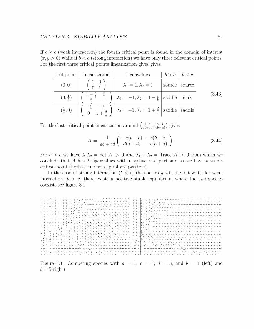
CHAPTER 3. STABILITY ANALYSIS 82
If b ≥ c (weak interaction) the fourth critical point is found in the domain of interest(x, y > 0) while if b < c (strong interaction) we have only three relevant critical points.For the first three critical points linearization gives gives
crit.point linearization eigenvalues b > c b < c
(0, 0)
(1 00 1
)λ1 = 1, λ2 = 1 source source
(0, 1b)
(1− c
b0
db
−1
)λ1 = −1, λ2 = 1− c
bsaddle sink
( 1a, 0)
(−1 − c
a
0 1 + da
)λ1 = −1, λ2 = 1 + d
asaddle saddle
(3.43)
For the last critical point linearization around(
b−cab+cd
, a+dab+cd
)gives
A =1
ab+ cd
(−a(b− c) −c(b− c)d(a+ d) −b(a+ d)
). (3.44)
For b > c we have λ1λ2 = det(A) > 0 and λ1 + λ2 = Trace(A) < 0 from which weconclude that A has 2 eigenvalues with negative real part and so we have a stablecritical point (both a sink or a spiral are possible).
In the case of strong interaction (b < c) the species y will die out while for weakinteraction (b > c) there exists a positive stable equilibrium where the two speciescoexist, see figure 3.1
0 0.25 0.5 0.75 1 1.25 1.5 1.75 2
0.25
0.5
0.75
1
1.25
1.5
0 0.25 0.5 0.75 1 1.25 1.5 1.75 2
0.25
0.5
0.75
1
1.25
1.5
Figure 3.1: Competing species with a = 1, c = 3, d = 3, and b = 1 (left) andb = 5(right)
CHAPTER 3. STABILITY ANALYSIS 83
3.2 Stable and unstable manifold theorem
We continue our investigation of the behavior of solutions near a critical point of thenonlinear equation x′ = f(x), where f is of class C1. As we have seen in Section 3.1we can always assume that the critical point is 0 and that the equation has the form
x′ = Ax+ g(x) , (3.45)
and g(x) = f(x) − dfdx
(0)x satisfies g(0) = 0 and dgdx
(0) = 0. Moreover for any ε > 0there exists δ > 0 such that ‖x‖ < δ, ‖y‖ < δ implies that ‖g(x)− g(y)‖ ≤ ε‖x− y‖.
Definition 3.2.1 A critical point a for the ODE x′ = f(x) is called hyperbolic if thematrix A = df
dx(a) has no eigenvalues with zero real part.
Let 0 be an hyperbolic critical point for the linear equation x′ = Ax, where x ∈ Rn
and A has k eigenvalues with negative real part and n − k eigenvalues with positivereal parts (counting multiplicities). We can split Rn into invariant stable and unstablesubspace, Rn = Es ⊗Eu with dimEs = k and dimEu = n− k. For any point x in thestable subspace Es we have limt→∞ ‖x(t)‖ = 0 and the convergence is exponentiallyfast. For any point in the unstable subspace Eu we have limt→−∞ ‖x(t)‖ = 0 and theconvergence is also exponentially fast.
We will show that the situation is essentially the same for the nonlinear equationx′ = Ax + f(x) in a neighborhood of an hyperbolic critical points: There exists ainvariant manifold (in fact a k-dimensional hypersurface)W s (the local stable manifold)defined locally around the origin which is tangent to Es and such that any solution ofx′ = Ax+f(x) which starts on W u converges exponential fast to 0 as t→∞. Similarlythere exists a manifold W s of dimension n− k, tangent to Es at the origin, such thatsuch that any solution of x′ = Ax + f(x) which starts on W s converges exponentialfast to 0 as t→∞.
We can always find an invertible C such that C−1AC is block diagonal
B = C−1AC =
(P 00 Q
). (3.46)
and the eigenvalues of the k×k matrix P have all negative real parts and the eigenvaluesof the n−k×n−k matrix Q have all positive real parts. If we set x = Cy, the equationbecomes
y′ = By + h(y) (3.47)
and h(y) = C−1g(Cy) has the same properties as g.
Theorem 3.2.2 Stable Manifold Theorem Let A be a n×n matrix with k eigenvalueswith negative real part and n− k eigenvalues with positive real parts. Let g : U → Rn
CHAPTER 3. STABILITY ANALYSIS 84
(U is a neighborhood of the origin) be a function of class C1 which satisfy g(0) = 0,g′(0) = 0, and for any ε > 0 there exists δ > 0 such that
‖g(x)− g(y)‖ ≤ ε‖x− y‖ , whenever ‖x‖ < δ , ‖y‖ < δ . (3.48)
Consider the ODEx′ = Ax+ g(x) . (3.49)
Then there exists a manifold W s (the local stable manifold) which is invariant underthe flow of (3.49) and contains the origin. Any solution of (3.49) which start on W s
converges exponential fast to 0 as t → ∞. Moreover there exists a manifold W u (thelocal unstable manifold) which is invariant under the flow of (3.49) and contains theorigin. Any solution of (3.49) which start on W u converges exponential fast to 0 ast→ −∞.
Proof: We can always find an invertible C such that C−1AC is block diagonal
B = C−1AC =
(P 00 Q
). (3.50)
and the eigenvalues of the k×k matrix P have all negative real parts and the eigenvaluesof the n−k×n−k matrix Q have all positive real parts. If we set x = Cy, the equationbecomes
y′ = By + h(y) (3.51)
and h(y) = C−1g(Cy) has the same condition as g does.We will construct W u for (3.51) as the graph of a function Ψ : Rk → Rn−k. The
equationsyj = Ψj(y1, · · · , yk) , j = k + 1, · · · , n . (3.52)
define a k-dimensional hypersurface in the y-space Rn. The unstable manifold in x-space for (3.49) is then obtained by the linear change of variables x = Cy.
Let us define
U(t) =
(ePt 00 0
), V (t) =
(0 00 eQt
). (3.53)
Then we haveeBt = U(t) + V (t) , (3.54)
andU ′(t) = PU(t) = BU(t) , V ′(t) = QV (t) = BV (t) . (3.55)
Since all eigenvalues of P (resp Q) have negative (resp. positive) real parts, we setα = maxReλj<0 Reλi and choose σ sufficiently small such that
‖U(t)‖ ≤ Ke−(α+σ)t , for all t ≥ 0 ,
‖U(t)‖ ≤ Keσt , for all t ≤ 0 . (3.56)
CHAPTER 3. STABILITY ANALYSIS 85
Nest consider the integral equation
u(t, a) = U(t)a+∫ t
0U(t− s)h(u(s, a)) ds−
∫ ∞t
V (t− s)h(u(s, a)) ds . (3.57)
By differentiating and using (3.55) one sees easily that if u(t, a) is a continuous solutionof the integral equation (3.57), then it is also a solution of y′ = Ay + h(y). We solvethis integral equation by the methods of successive approximations with
u0(t, a) = 0 ,
u(m+1)(t, a) = U(t)a+∫ t
0U(t− s)h(u(m)(s, a)) ds−
∫ ∞t
V (t− s)h(u(m)(s, a)) ds .
We assume that ε ≤ σ/4k and ‖a‖ ≤ δ/2K where ε and δ are given by the Lipschitz-type condition on h. We show then by induction that
‖u(m)(t, a)‖ ≤ 2K‖a‖e−αt , (3.58)
‖u(m)(t, a)− u(m−1)(t, a)‖ ≤ K‖a‖e−αt
2m−1, for t ≥ 0. (3.59)
Let us assume that (3.58) holds for u(m)(t, a). Then, ‖u(m)(t, a)‖ ≤ 2K‖a‖ ≤ δ and so,using that ‖h(y)‖ ≤ ε‖y‖ if ‖y‖ ≤ δ and the bounds on U(t) and V (t) we have
‖u(m+1)(t, a)‖
≤ ‖U(t)‖‖a‖+ ε∫ t
0‖U(t− s)‖‖u(m)s, a)‖ ds+ ε
∫ ∞t‖V (t− s)‖‖u(m)(s, a)‖ ds
≤ Ke−(α+σ)t‖a‖+ 2εK2‖a‖∫ t
0e−(α+σ)(t−s)e−αs ds+ 2εK2‖a‖
∫ ∞t
eσ(t−s)e−αs ds
≤ Ke−(α+σ)t‖a‖+ 2εK2e−αt1
σ+ 2εK2e−αt
1
α + σ≤ 2Ke−αt , (3.60)
where in the last inequality we have used that ε ≤ σ/4K.Let us consider next (3.59). It holds for m = 1 because h(0) = 0 and because of the
bound on ‖U(t)‖. Since u(m)(t, a) ≤ 2K‖a‖ ≤ δ we use that ‖h(y)− h(z)‖ ≤ ε‖y − z‖if ‖y‖, ‖z‖ ≤ δ and we have, by the induction hypothesis,
‖u(m+1)(t, a)− u(m)(t, a)‖‖un(s, a)− un−1(s, a)‖ ds‖un(s, a)− un−1(s, a)‖ds
≤ ε∫ t
0Ke−(α+σ)(t−s)K‖a‖e−αs
2m−1ds + ε
∫ ∞t
eσ(t−s)K‖a‖e−αs
2m−1ds
≤ εK2‖a‖2n−1
(e−(α+σ)t
∫ t
0eσs ds+ eσt
∫ ∞t
e−(α+σ)s ds)
≤ εK2‖a‖e−αt
2m−1
(1
σ+
1
σ + α
)≤ K‖a‖e−αt
2m, (3.61)
CHAPTER 3. STABILITY ANALYSIS 86
where, in the last inequality, we assume that ε < σ/4K.The bound (3.59) and using telescopic sum implies that for k > m and t > 0
‖u(k)(t, a)− u(m)(t, a)‖ ≤ K‖a‖∞∑j=m
1
2j, (3.62)
and thus {u(m)(t, a)} is a Cauchy sequence uniformly in t > 0. Thus u(t, a) =limn→∞ u
(m)(t, a) is continuous and satisfies the integral equation (3.57). Moreoverby (3.58), u(t, a) satisfies the bound
‖u(t, a)‖ ≤ 2Ke−αt , for t ≥ 0 and ‖a‖ ≤ δ/2K . (3.63)
From the form of the integral equation (3.57), it is clear that the last n − k com-ponents of the vector a do not enter the computation and hence they may and willbe taken to be 0. The components of u(t, a) = (u1(t, a), · · ·un(t, a)) satisfy the initialconditions
uj(0, a) = aj for j = 1, · · · , k . (3.64)
and
uj(0, a) = −∫ ∞
0V (−s)h(u(s, a1, · · · , ak, 0, · · · 0)) for j = k + 1, · · · , n . (3.65)
Now we define the function Ψ = (ψj+1, · · · , ψn) by
ψj(a1, · · · , ak) = uj(0, a1, · · · , ak) . (3.66)
The map Ψ is defined in a neighborhood of the origin and define a n− k dimensionalhypersurface S yj = Ψj(y1, cdots, yk).
If y(t) is a solution of y′ = By + h(y) with y(0) ∈ S, i.e., y(0) = u(0, a) theny(t) = u(t, a) and by (3.63) limt→∞ y(t) = 0.
On the other hand if y(t) is a solution with ‖y(0)‖ small and y(0) not on S, theny(t) will exit the ball {‖y‖ ≤ δ}. By contradiction suppose that y(t) ≤ δ for all t ≥ 0.Then we have
y(t) = eBty(0) +∫ ∞
0eB(t−s)h(y(s)) ds
= U(t)y(0) + V (t)c+∫ t
0U(t− s)h(y(s)) ds−
∫ ∞t
V (t− s)h(y(s)) ds .(3.67)
where c is the vectorc = y(0) +
∫ ∞0
V (−s)h(y(s)) ds . (3.68)
The integral in (3.68) converges by the bound on ‖V (t)‖ and since h(y(s)) is bounded.Then all terms in (3.67) are uniformly bounded in t except possible the term V (t)c.

CHAPTER 3. STABILITY ANALYSIS 87
Since all eigenvalues of q have positive real parts, we have ‖V (t)‖ ≥ eγt. Thus V (t)c isunbounded unless c = 0. But if c = 0, y(0) ∈ S which is a contradiction.
The existence of an unstable manifold is proved exactly in the same way by reversingtime t 7→ −t, i.e., by considering the system
y′ = −By − h(y) . (3.69)
The stable manifold for (3.69) is the unstable manifold for y′ = By + h(y). Thisconcludes the proof of the theorem.
Remark 3.2.3 With a little more work one can show that the function Ψj are differ-entiable. This is similar to the proof that solution are differentiable with respect tothe initial conditions. We will not do it here. We will show however that if we assumethe map Ψ to be differentiable, then the stable manifold W s is tangent to the stablesubspace Es of y′ = By which is yj+1 = · · · yn = 0. To see this we not that Ψj(0, 0) = 0and
|ψj(0, a)| =∣∣∣∣∫ ∞
0V (−s)h(u(s, a)) ds
∣∣∣∣ ≤ 2εK2‖a‖/σ . (3.70)
Since ε can be made arbitrarily small by choosing ‖a‖ small enough, this shows that∂ψj∂yi
(0) = 0. And so W s is tangent to Es.
Example 3.2.4 The proof of the stable manifold theorem provides an algorithm toconstruct the stable and unstable manifold. Let us consider the system
x′1 = −x1 − x22 ,
x′2 = x2 + x21 . (3.71)
Here A =
(−1 00 1
)is already in Jordan normal form. So we have
U(t) =
(e−t 00 0
), V (t) =
(0 00 et
). (3.72)
and we can take a = (a1, 0)T . The integral equation for u(t, a) is given by
u(t, a) =
(e−ta1
0
)−∫ t
0
(e−(t−s)u2
2(s)0
)ds −
∫ ∞t
(0
e(t−s)u1(s)
)ds . (3.73)
Therefore we find
u(0)(t, a) = 0 ,
u(1)(t, a) =
(e−ta1
0
),
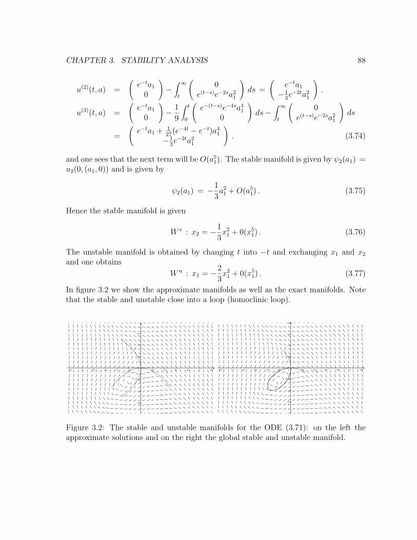
CHAPTER 3. STABILITY ANALYSIS 88
u(2)(t, a) =
(e−ta1
0
)−∫ ∞t
(0
e(t−s)e−2sa21
)ds =
(e−ta1
−13e−2ta2
1
).
u(3)(t, a) =
(e−ta1
0
)− 1
9
∫ t
0
(e−(t−s)e−4sa4
1
0
)ds−
∫ ∞t
(0
e(t−s)e−2sa21
)ds
=
(e−ta1 + 1
27(e−4t − e−t)a4
1
−13e−2ta2
1
). (3.74)
and one sees that the next term will be O(a51). The stable manifold is given by ψ2(a1) =
u2(0, (a1, 0)) and is given by
ψ2(a1) = −1
3a2
1 +O(a51) . (3.75)
Hence the stable manifold is given
W s : x2 = −1
3x2
1 + 0(x51) . (3.76)
The unstable manifold is obtained by changing t into −t and exchanging x1 and x2
and one obtains
W u : x1 = −2
3x2
1 + 0(x51) . (3.77)
In figure 3.2 we show the approximate manifolds as well as the exact manifolds. Notethat the stable and unstable close into a loop (homoclinic loop).
-4.8 -4 -3.2 -2.4 -1.6 -0.8 0 0.8 1.6 2.4 3.2 4 4.8
-2.4
-1.6
-0.8
0.8
1.6
2.4
-4.8 -4 -3.2 -2.4 -1.6 -0.8 0 0.8 1.6 2.4 3.2 4 4.8
-3.2
-2.4
-1.6
-0.8
0.8
1.6
2.4
3.2
Figure 3.2: The stable and unstable manifolds for the ODE (3.71): on the left theapproximate solutions and on the right the global stable and unstable manifold.
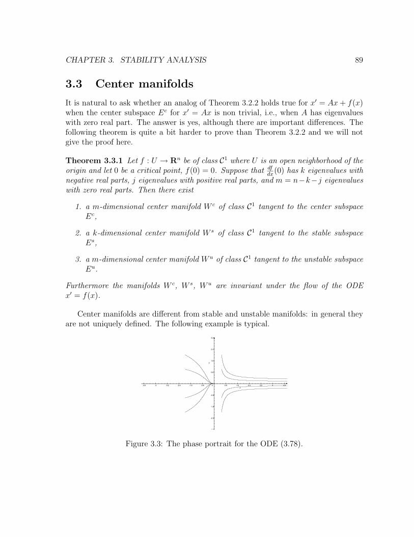
CHAPTER 3. STABILITY ANALYSIS 89
3.3 Center manifolds
It is natural to ask whether an analog of Theorem 3.2.2 holds true for x′ = Ax+ f(x)when the center subspace Ec for x′ = Ax is non trivial, i.e., when A has eigenvalueswith zero real part. The answer is yes, although there are important differences. Thefollowing theorem is quite a bit harder to prove than Theorem 3.2.2 and we will notgive the proof here.
Theorem 3.3.1 Let f : U → Rn be of class C1 where U is an open neighborhood of theorigin and let 0 be a critical point, f(0) = 0. Suppose that df
dx(0) has k eigenvalues with
negative real parts, j eigenvalues with positive real parts, and m = n−k−j eigenvalueswith zero real parts. Then there exist
1. a m-dimensional center manifold W c of class C1 tangent to the center subspaceEc,
2. a k-dimensional center manifold W s of class C1 tangent to the stable subspaceEs,
3. a m-dimensional center manifold W u of class C1 tangent to the unstable subspaceEu.
Furthermore the manifolds W c, W s, W u are invariant under the flow of the ODEx′ = f(x).
Center manifolds are different from stable and unstable manifolds: in general theyare not uniquely defined. The following example is typical.
-4.8 -4 -3.2 -2.4 -1.6 -0.8 0 0.8 1.6 2.4 3.2 4 4.8
-3.2
-2.4
-1.6
-0.8
0.8
1.6
2.4
3.2
Figure 3.3: The phase portrait for the ODE (3.78).
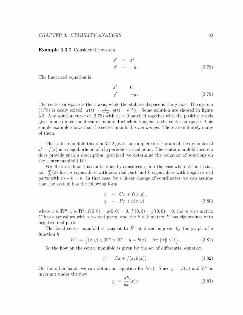
CHAPTER 3. STABILITY ANALYSIS 90
Example 3.3.2 Consider the system
x′ = x2 ,
y′ = −y . (3.78)
The linearized equation is
x′ = 0 ,
y′ = −y . (3.79)
The center subspace is the x-axis, while the stable subspace is the y-axis. The system(3.78) is easily solved: x(t) = 1
t−x0, y(t) = e−ty0. Some solution are showed in figure
3.3. Any solution curve of (3.78) with x0 < 0 patched together with the positive x-axisgives a one-dimensional center manifold which is tangent to the center subspace. Thissimple example shows that the center manifold is not unique. There are infinitely manyof them.
The stable manifold theorem 3.2.2 gives a a complete description of the dynamics ofx′ = f(x) in a neighborhood of a hyperbolic critical point. The center manifold theoremdoes provide such a description; provided we determine the behavior of solutions onthe center manifold W c.
We illustrate how this can be done by considering first the case where Eu is trivial,i.e., df
dx(0) has m eigenvalues with zero real part and k eigenvalues with negative real
parts with m+ k = n. In that case, by a linear change of coordinates, we can assumethat the system has the following form
x′ = Cx+ f(x, y) ,
y′ = Px+ g(x, y) . (3.80)
where x ∈ Rm, y ∈ Rk, f(0, 0) = g(0, 0) = 0, f ′(0, 0) = g′(0, 0) = 0, the m×m matrixC has eigenvalues with zero real parts, and the k × k matrix P has eigenvalues withnegative real parts.
The local center manifold is tangent to Ec at 0 and is given by the graph of afunction h
W c ={
(x, y) ∈ Rm ×Rk : y = h(x) for ‖x‖ ≤ δ}. (3.81)
So the flow on the center manifold is given by the set of differential equation
x′ = Cx+ f(x, h(x)) . (3.82)
On the other hand, we can obtain an equation for h(x). Since y = h(x) and W c isinvariant under the flow
y′ =dh
dx(x)x′ (3.83)
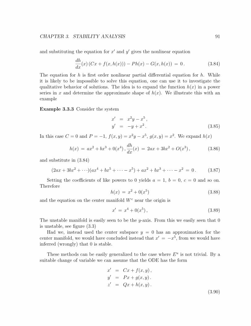
CHAPTER 3. STABILITY ANALYSIS 91
and substituting the equation for x′ and y′ gives the nonlinear equation
dh
dx(x) (Cx+ f(x, h(x)))− Ph(x)−G(x, h(x)) = 0 . (3.84)
The equation for h is first order nonlinear partial differential equation for h. Whileit is likely to be impossible to solve this equation, one can use it to investigate thequalitative behavior of solutions. The idea is to expand the function h(x) in a powerseries in x and determine the approximate shape of h(x). We illustrate this with anexample
Example 3.3.3 Consider the system
x′ = x2y − x5 ,
y′ = −y + x2 . (3.85)
In this case C = 0 and P = −1, f(x, y) = x2y − x5, g(x, y) = x2. We expand h(x)
h(x) = ax2 + bx3 + 0(x4) ,dh
dx(x) = 2ax+ 3bx2 +O(x3) , (3.86)
and substitute in (3.84)
(2ax+ 3bx2 + · · ·)(ax4 + bx5 + · · · − x5) + ax2 + bx3 + · · · − x2 = 0 . (3.87)
Setting the coefficients of like powers to 0 yields a = 1, b = 0, c = 0 and so on.Therefore
h(x) = x2 + 0(x5) (3.88)
and the equation on the center manifold W c near the origin is
x′ = x4 + 0(x5) , (3.89)
The unstable manifold is easily seen to be the y-axis. From this we easily seen that 0is unstable, see figure (3.3)
Had we, instead used the center subspace y = 0 has an approximation for thecenter manifold, we would have concluded instead that x′ = −x5, from we would haveinferred (wrongly) that 0 is stable.
These methods can be easily generalized to the case where Eu is not trivial. By asuitable change of variable we can assume that the ODE has the form
x′ = Cx+ f(x, y) ,
y′ = Px+ g(x, y) .
z′ = Qx+ h(x, y) .
(3.90)
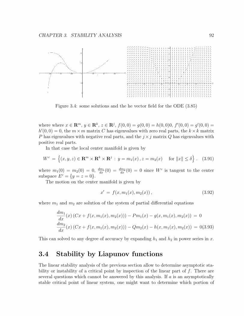
CHAPTER 3. STABILITY ANALYSIS 92
-1.25 -1 -0.75 -0.5 -0.25 0 0.25 0.5 0.75 1 1.25
-0.16
-0.08
0.08
0.16
0.24
0.32
0.4
0.48
Figure 3.4: some solutions and the he vector field for the ODE (3.85)
where where x ∈ Rm, y ∈ Rk, z ∈ Rj, f(0, 0) = g(0, 0) = h(0, 0)0, f ′(0, 0) = g′(0, 0) =h′(0, 0) = 0, the m×m matrix C has eigenvalues with zero real parts, the k×k matrixP has eigenvalues with negative real parts, and the j×j matrix Q has eigenvalues withpositive real parts.
In that case the local center manifold is given by
W c ={
(x, y, z) ∈ Rm ×Rk ×Rj : y = m1(x) , z = m2(x) for ‖x‖ ≤ δ}. (3.91)
where m1(0) = m2(0) = 0, dm1
dx(0) = dm2
dx(0) = 0 since W c is tangent to the center
subspace Ec = {y = z = 0}.The motion on the center manifold is given by
x′ = f(x,m1(x),m2(x)) , (3.92)
where m1 and m2 are solution of the system of partial differential equations
dm1
dx(x) (Cx+ f(x,m1(x),m2(x)))− Pm1(x)− g(x,m1(x),m2(x)) = 0
dm2
dx(x) (Cx+ f(x,m1(x),m2(x)))−Qm2(x)− h(x,m1(x),m2(x)) = 0 .(3.93)
This can solved to any degree of accuracy by expanding h1 and h2 in power series in x.
3.4 Stability by Liapunov functions
The linear stability analysis of the previous section allow to determine asymptotic sta-bility or instability of a critical point by inspection of the linear part of f . There areseveral questions which cannot be answered by this analysis. If a is an asymptoticallystable critical point of linear system, one might want to determine which portion of
CHAPTER 3. STABILITY ANALYSIS 93
phase space actually converges to the critical point (i.e., determine its basin of attrac-tion). Another question is to determine the stability of critical point for which someof the eigenvalues of the linearization have a zero real part. In that case the linearstability analysis of the previous section is inconclusive.
Let us consider the autonomous equation
x′ = f(x) , (3.94)
where f is locally Lipschitz in an open set U . We assume that 0 ∈ U and f(0) = 0.The zero solution x(t) = 0 is an equilibrium state. The extension to an equilibriumstate x(t) = a is elementary.
We call a function V : D → R, where D is an open neighborhood of 0, a Liapunovfunction if V (0) = 0 and V (x) > 0 for x ∈ D, x 6= 0.
We recall that the derivative of V along a solution x(t) is given by
d
dtV (x(t)) =≡
n∑j=1
∂V
∂xj(x(t))x′i(t) = 〈∇V (x(t)) , f(x(t))〉 . (3.95)
We setLV (x) = 〈∇V (x) , f(x)〉 . (3.96)
We also introduce the concept of exponential stability of a solution.
Definition 3.4.1 A solution x(t, t0, x0) is exponentially stable if there exists constantsc, γ > 0 and δ > 0 such that ‖ξ‖ ≤ δ implies that
‖x(t, t0, x0 + ξ)− x(t, t0, x0)‖ ≤ ce−γ(t−t0) . (3.97)
Clearly exponential stability implies asymptotic stability. For linear equation asymp-totic stability and exponential stability are equivalent.
Theorem 3.4.2 (Stability Theorem of Liapunov) Let f : U → Rn (U an openset of Rn) be locally Lipschitz with f(0) = 0. Let V be a Liapunov function defined inan open neighborhood D of 0
1. If LV ≤ 0 in D then 0 is a stable critical point.
2. If LV < 0 in D \ {0} then 0 is asymptotically stable critical point.
3. if LV ≤ −αV and V (x) ≥ a‖x‖β in D (α, β, a are positive constants) then 0 anexponentially stable critical point.
CHAPTER 3. STABILITY ANALYSIS 94
Proof: 1. Choose η so small that the set Vη ≡ {x ; V (x) < η} is contained in D. SinceV (x) > 0 for x 6= 0 Vη is an open neighborhood of 0. Since LV ≤ 0 in Vη ⊂ D,if x0 ∈ Vη then the solution x(t, 0, x0) exists for all t ≥ t0 and it does not leave Vηever. This implies stability since for η small enough we can choose δ and ε such that{‖x‖ < δ} ⊂ Vη ⊂ {‖x‖ < ε}.
2. By 1. we know that for η sufficiently small x(t, t0, x0) stay in Vη for all times.Moreover V (x(t, t0, x0)) is a positive decreasing function so that limt→∞ V (x(t)) = V ∗
exists. Let us assume that V ∗ 6= 0. The set M = {V ∗ ≤ V (x) ≤ η} is a compactset which does not contain 0. We have x(t) ∈ M , for all t > t0 and maxx∈M LV (x) ≤−α < 0. So dV
dt(x(t)) ≤ −α for all t > t0 which is a contradiction. So we must have
V ∗ = 0 and limt→∞ ‖x(t)‖ = 0.3. We have dV
dt(x(t)) ≤ −αV (x(t))and thus, by Gronwall Lemma, V (x(t)) ≤
V (x(t0))e−α(t−t0). Since b‖x(t)‖β ≤ V (x(t)) we obtain ‖x(t)‖ ≤ V (x(t0))b
e−αβ
(t−t0) andthis proves exponential stability.
Theorem 3.4.3 (Instability theorem of Liapunov) Let f : U → Rn (U an openset of Rn) be locally Lipschitz with f(0) = 0. Let V be a function defined in an openneighborhood D of 0 (V is not necessarily positive) which satisfies
1. lim‖x‖→0 V (x) = 0.
2. LV (x) > 0 if x ∈ D \ {0}.
3. V (x) takes positive values in each sufficiently small neighborhood of 0.
Then 0 is unstable.
Remark 3.4.4 The conditions 1 and 3 of Theorem 3.4.3 are satisfied, in particular, ifV is a Liapunov function, i.e., V (0) = 0 and V (x) > 0, x ∈ D \ {0}.
Proof: Stability means that for any ε > 0, there exists δ > 0 such that ‖x0‖ ≤ δ impliesthat ‖x(t, 0, x0)‖ ≤ ε for all t > 0.
Let us choose ε > 0 such that the set {x ; ‖x‖ ≤ ε} ⊂ D. Now for arbitrary δ > 0,by assumptions 1 and 3 we can find x0 such that ‖x0‖ ≤ δ and V (x0) = α > 0.By assumption 2, LV > 0, so that V (x(t)) ≥ α for all t ≥ 0. The set {x ; ‖x‖ ≤ε and V (x) ≥ α} does not contain the origin and therefore there exists β > 0 suchthat, in this set, LV (x) ≥ β. We thus obtain that
V (x(t))− V (x(0)) =∫ t
0LV (x(s)) ds ≥ βt , (3.98)
orV (x(t)) ≥ α + βt (3.99)
as long as ‖x(t)‖ ≤ ε. This implies that x(t) actually exits the balls {x ; ‖x‖ ≤ ε}.Since δ is arbitrary we conclude that 0 is unstable.
CHAPTER 3. STABILITY ANALYSIS 95
Example 3.4.5 Consider the system of equations
x′ = ax− y + kx(x2 + y2) ,
y′ = x− ay + ky(x2 + y2) (3.100)
where a > 0 and k are constants. Clearly (0, 0) is a critical point and the linearizationgives
A =
(a −11 −a
)with eigenvalues λ = ±(a2 − 1) . (3.101)
and so we have
1. If a2 > 1 then 0 is a saddle point and it is unstable by Theorem 3.1.2.
2. If a2 = 1 the system is degenerate.
3. If a2 < 1 then the eigenvalues are purely imaginary and we have a center (vortex).
In order to study the case a2 < 1 we construct a Liapunov function. The linearizedsystem x′ = Ax has orbits which are the ellipses
V (x, y) = x2 − 2axy + y2 = c . (3.102)
It is quite natural to take V (x, y) a Liapunov function to study the effect of the non-linear terms. We have
LV = (2x− 2ay)kx(x2 + y2) + (2y − 2ax)ky(x2 + y2)
= 2k(x2 + y2)(x2 + y2 − 2axy) . (3.103)
We conclude from Theorem 3.4.3 that 0 is unstable if k > 0 and from Theorem 3.4.2that 0 is asymptotically stable for k < 0.
If a is a asymptotically stable critical point, then all solutions starting in a neigh-borhood of a converge to a as t goes to infinity. We call a an attracting point or anattractor. The basin of attraction of a is the set of point y such that x(t, 0, y) → a ast→∞. Liapunov functions are useful to determine, or at least estimate, the basin ofattraction of a critical point.
For example, if V is a Liapunov function in a neighborhood D of a and LV < 0 inD \ a, then D is the basin of attraction of a.
Example 3.4.6 Consider the system
x′ = −x3 ,
y′ = −y(x2 + z2 + 1)
x′ = − sin(z) (3.104)
CHAPTER 3. STABILITY ANALYSIS 96
The critical points are (0, 0, nπ) with n = 0,±1,±2, · · ·. Note that if z = nπ thenz′ = 0 and thus the planes z = nπ are invariant. Any solution which starts in suchplane stays in this plane for all time t ∈ R. This implies that any solution whichstarts in the region |z| < π stays in this region for ever. Let us study the stability of0 = (0, 0, 0). The linearization around 0 gives the linear system with
A =
0 0 00 −1 00 0 −1
(3.105)
and this tells us nothing about the stability of this equilibrium point. However let usconsider the function V (x, y, z) = x2 + y2 + z2. We have
LV = −2x4 − 2y2(x2 + y2 + z2)− 2z sin(z) (3.106)
For |z| < π, LV < 0 except at the origin. It follows from Theorem 3.4.2 that the basinof attraction of 0 is the entire region {(x, y, z), |z| < π}.
In many interesting examples, however, LV = 0 in some subset of D but never-theless a is asymptotically stable and to study this we are going to prove a strongerversion of the Liapunov stability theorem.
Theorem 3.4.7 (Lasalle Stability Theorem) Let f : U → Rn (U an open set ofRn) be locally Lipschitz with f(0) = 0. Let V be a Liapunov function defined in anopen neighborhood D of 0 and let us assume that the set G = {x ; V (x) ≤ α, x ∈ D}is compact for some α > 0. Let us assume that LV (x) ≤ 0 for x ∈ G and that there isno solution x(t), t ∈ R with x0 ∈ G on which V is constant. Then 0 is asymptoticallystable and Vα is contained in the basin of attraction of 0.
Proof: Let x0 ∈ G, then x(t) = x(t, 0, x0) ∈ G for all t > 0. This follows from thefact that LV ≤ 0 in G and from the compactness of G (the distance from G to theboundary of D is positive).
The proof is by contradiction. Let us assume that x(t) does not tend to 0. Since x(t)stays in the compact set G there exists a sequence tn →∞ so that limn→∞ x(tn) = x∗
with x∗ ∈ G.We claim that the solution y(t) = x(t, 0, x∗) starting at x∗ exists for all t ∈ R and
stays in the set G. Clearly y(t) exists for all positive t. On the other hand x(t, 0, x(tn))is defined for all t ∈ [−tn, 0]. Since tn is an increasing sequence then, for any k ≥ 1,x(t, 0, x(tn+k)) is also defined for all t ∈ [−tn, 0]. By the continuous dependence oninitial conditions we have that y(t) = x(t, 0, x∗) is defined for t ∈ [−tn, 0]. Since n isarbitrary and tn →∞ this proves the claim.
We show next that V is constant on the solution y(t) = x(t, 0, x∗). If V (x∗) = bthen V (x(tn)) ≥ b and limn→∞ V (xtn) = b. More generally for any sequence sn with
CHAPTER 3. STABILITY ANALYSIS 97
limn→∞ sn = ∞ we have limn→∞ V (xsn) = b. This follows from the fact that V isnonincreasing along a solution. With sn = s + tn we have limn→∞ x(sn) = y(s) =x(s, 0, x∗) and therefore V (x(s, 0, x∗)) = b. Since s is arbitrary this proves the claim.
This contradicts our assumption that V is not constant on any solution.
Example 3.4.8 Consider the equation x′′ + x′ + x3 = 0, or x′ = y and y′ = −y− x3
The equation x′′ + x3 is Hamiltonian with Hamiltonian y2/2 + x4/4. The term x′ = yis a friction term and one expects that 0 is an attracting fixed point with basin ofattraction R2. Using the Liapunov function H(x, y) we find that LH = −y2, i.e,. LHis non-positive but vanishes on the line y = 0. To apply Lasalle theorem we show thatH does not stay constant on any solution, except the trivial solution. By contradiction,assume that H(x(t), y(t)) is constant then LH(x(t), y(t)) = 0 and thus y(t) = 0. Theequation y′ = −y− x3 implies then that x(t) = 0 and this contradicts our assumptionthat the solution is not trivial. Lasalle Theorem implies that (0, 0) is asymptoticallystable and that its basin of attraction is the entire plane R2.
3.5 Gradient and Hamiltonian systems
There are several classes of systems where the use of Liapunov functions is very natural.
3.5.1 Gradient systems
Let V : U → R (U is an open set of Rn) be a function of class C2. A gradient systemon U ⊂ Rn is a differential equation of the form
x′ = −∇V (x) . (3.107)
(The negative sign is a traditional convention). The equilibrium points for (3.107) arethe critical points of V , i.e., the points a for which ∇V (a) = 0.
Consider the level sets of the function V , V −1(c) = {x ;V (x) = c}. If x ∈ V −1(c)is a regular point, i.e., if ∇V (x) 6= 0, then, by the implicit function Theorem, locallynear x, V −1(c) is a smooth hypersurface surface of dimension n − 1. For example, ifn = 2, the level sets are smooth curves.
We summarize the properties of the gradient systems in
Proposition 3.5.1 Let V : U → Rn (U an open set in Rn) be of class C2 and letx′ = −∇V (x) be a gradient system.
1. If x is a regular point of the level curve V −1(c), then the solution curve x(t) isperpendicular to the level surface V −1(c).
CHAPTER 3. STABILITY ANALYSIS 98
2. If a is an isolated minimum of V , then it a is an asymptotically stable criticalpoint.
3. If a is an isolated minimum of V or a saddle point of V , then a is an unstablecritical point.
Proof: Let y be a vector which is tangent to the level surface V −1(c) at the point x.For any curve γ(t) in the level set V −1(c) with γ(0) = x and γ′(0) = y we have
0 =d
dtV (γ(t))|t=0 = 〈∇V (x) , y〉 , (3.108)
and so ∇V (x) is perpendicular to any tangent vector to the level set V −1(c) at allregular points of V . This proves 1.
If x(t) is a solution of (3.107), then we have
d
dtV (x(t)) = −〈∇V (x(t)) , ∇V (x(t))〉 ≤ 0 . (3.109)
If a is an isolated minimum of V , then consider the Liapunov function W (x) = V (x)−V (a). We have LW (x) < 0 in a neighborhood of a and so, by Theorem 3.4.2, a is anasymptotically stable equilibrium point. This proves 2. If If a is an isolated minimumof V or a saddle point of V , we consider the function W (x) = V (a) − V (x). If a is aisolated minimum W (x) is a Liapunov function and if a is a saddle point then W (x)satisfy the conditions 1 and 3 of Theorem 3.4.3. In both case we have LW > 0 in aneighborhood of a and thus, by Theorem 3.4.3, a is unstable. This proves 3.
Example 3.5.2 Let V : R2 → R be the function V (x, y) = x2(x− 1)2 + y2
2. The the
gradient system is given by
x′ = −2x(x− 1)(2x− 1) ,
y′ = −y . (3.110)
There are 3 critical points (0, 0), (0, 1/2, 0), and (0, 1). From the form of V oneconcludes that (0, 0) and (0, 1) are asymptotically stable with basins of attraction{−∞ < x < 1/2 , −∞ < y < ∞} and {1/2 < x < ∞ , −∞ < y < ∞} respectively.The critical point (1, 0) is unstable (saddle point). The solution with initial condi-tions x(0) = 1 and y(0) = y0 satisfy (x(t), y(t)) → (0, 1). See figure 3.5.2 in the nextsubsection.
We also have
Proposition 3.5.3 Let V : U → Rn (U an open set in Rn) be of class C2 and letx′ = −∇V (x) be a gradient system. If a is a critical point, then the linearizationaround A has only real eigenvalues.
CHAPTER 3. STABILITY ANALYSIS 99
Proof: Let a be a critical point. Then the linearized system is given by the matrixA = (aij) where
aij = − ∂2
∂xi∂xj(a) . (3.111)
Since V is of class C2 we have aij = aji. Therefore A is a symmetric matrix and itseigenvalues are real.
3.5.2 Hamiltonian systems
Let x = (x1, · · · , xn) ∈ Rn and y = (y1, · · · , yn) ∈ Rn and let H : U → R (U an anopen set of R2n) be a function of class C2. For mechanical systems x are the coordinatesof the particles and y are the momenta of the particles. The function H(x, y) is calledthe energy or the Hamiltonian of the system.
A Hamiltonian system for the Hamiltonian H is a system of differential equationsof the form
x′i =∂H
∂yii = 1, · · · , n ,
y′i = −∂H∂xi
i = 1, · · · , n . (3.112)
A simple but very important property of Hamiltonian is conservation of energy
Proposition 3.5.4 Let H(x, y) be a function of class C2. Let (x(t), y(t)) be a solutionof the Hamilton equations (3.112), then H(x(t), y(t)) is constant.
Proof: We have
d
dtH(x(t), y(t)) =
n∑i=1
∂H
∂xix′i +
∂H
∂yiy′i
=n∑i=1
∂H
∂xi
∂H
∂yi− ∂H
∂yi
∂H
∂xi= 0 . (3.113)
Hence H is constant along any solution.
This means that any solution (x(t), y(t)) stays on the level set {H(x, y) = c =H(x(0), y(0))} of the Hamiltonian. If the level set of the Hamiltonian is compact, thenthe solution exists for all positive and negative times.
Let z = (x, y) and define J : R2n → R2n as the linear map given by
J =
(0 I−I 0
). (3.114)
CHAPTER 3. STABILITY ANALYSIS 100
where I is the n × n identity matrix. Note that we have JT = J−1 = −J . We canrewrite (3.113) as
z′ = J−1∇H(z) . (3.115)
Theorem 3.5.5 Let U ⊂ R2n be an open set and H : U → R be of class C2. Thenthe flow φt(z) = z(t, 0, z) for (3.115) satisfy
(∂φt
∂z
)TJ
(∂φt
∂z
)= J . (3.116)
Remark 3.5.6 A map T : U → R2n (U ⊂ R2n open) which satisfies ∂T∂x
TJ ∂T∂x
= J iscalled a symplectic transformation.
Proof: The derivative ∂φt
∂zis the solution for the variational equation, which is
Ψ′(t) = J−1d2H
dz2(z(t, 0, z))Ψ(t) , Ψ(0) = I , (3.117)
whered2H
dz2=
(∂2H
∂zi∂zj
)1≤i,j≤n
. (3.118)
is a symmetric matrix. We have then
d
dt
(∂φt
∂z
)TJ
(∂φt
∂z
)=
(∂φt∂z
)T′ J (∂φt∂z
)+
(∂φt
∂z
)TJ
(∂φt
∂z
)′
=
(∂φt
∂z
)Td2H
dz2(z(t, 0, z))J2
(∂φt
∂z
)+
(∂φt
∂z
)Td2H
dz2(z(t, 0, z))
(∂φt
∂z
)= 0 . (3.119)
Since (3.116) holds for t = 0 it holds thus for all t.
A direct consequence of the symplecticity of the flow is
Theorem 3.5.7 Let U ⊂ R2n be an open set and H : U → R be of class C2. The flowφt for (3.115) is volume preserving, i.e., for any A ⊂ Rn compact with ∂A negligiblewe have
vol(φt(A)
)= vol(A) . (3.120)
CHAPTER 3. STABILITY ANALYSIS 101
Proof: The map φt is of class C1 by Theorem (2.6.6) and injective by the uniqueness ofsolutions. Since detJ = 1, from Theorem 3.5.5 we have∣∣∣∣∣det
(∂φt
∂x
)∣∣∣∣∣ = 1 . (3.121)
By the change of variables formula we have
vol(φt(A)
)=∫ ∫
φt(A)dx dy =
∫ ∫φt(A)
dx dy =∫ ∫
A
∣∣∣∣∣det∂φt
∂x
∣∣∣∣∣ dx dy = vol(A) .
(3.122)and so φt preserves volume.
Remark 3.5.8 This can be derived directly from Liouville Theorem 2.1.6 (see home-work). The property of symplecticity is a much stronger than volume preserving, atleast for n ≥ 1.
Remark 3.5.9 Because of the volume preserving property critical points of Hamilto-nian systems are never asymptotically stable.
Theorem 3.5.10 Consider Hamilton’s equation (3.112) where H is of class C2. Leta be a critical point for (3.112). If H(x, y) − H(a) is positive (or negative) in aneighborhood of a then a is a stable critical point.
Proof: Without loss of generality we may assume that a = 0. By Proposition (3.5.4)V (x, y) = H(x, y) −H(0) (or V (x, y) = H(0) −H(x, y)) is a Liapunov function withLV = 0. The theorem follows immediately from item 1. of Theorem 3.4.2.
In mechanical systems, the Hamiltonian has (usually) the form H = T +W whereT is the kinetic energy and U is the potential energy. We have
T =n∑i=1
y2i
2, W = W (x) , (3.123)
in particular T is positive. The Hamiltonian equations have then the form (Newton’s2nd law)
x′′i = −∇W (x) . (3.124)
Equilibrium solutions then correspond to
y = 0 , ∇W (x) = 0 . (3.125)
We have
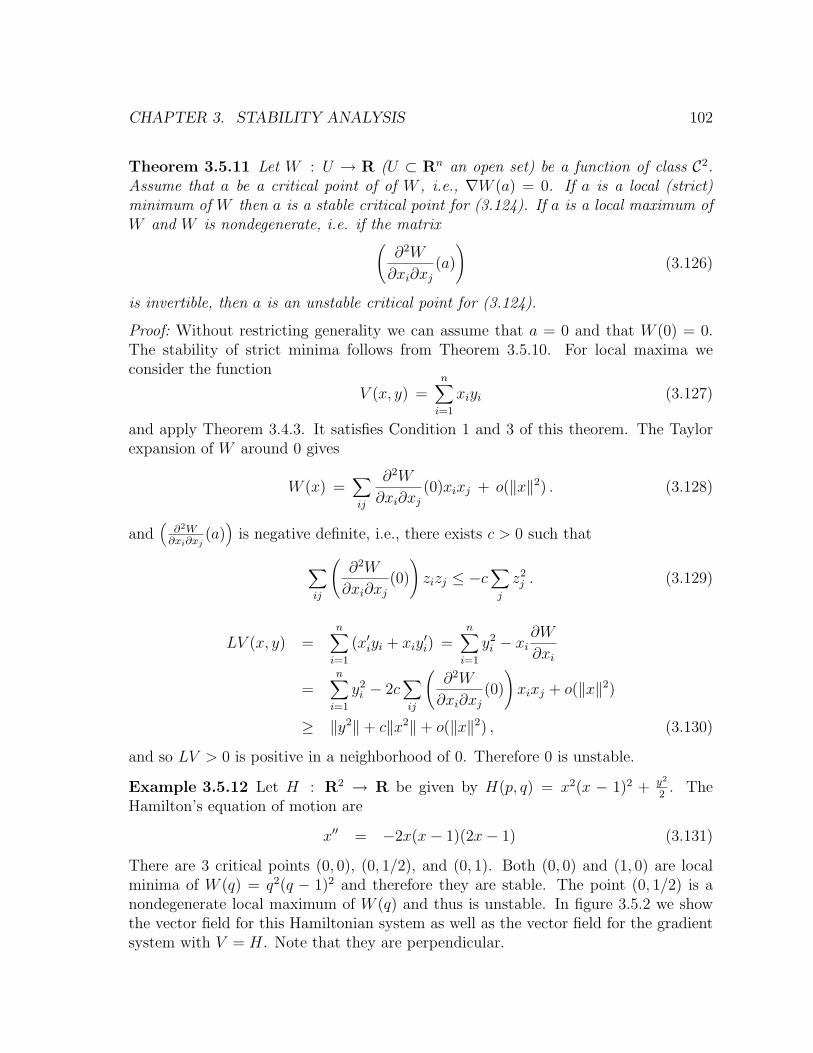
CHAPTER 3. STABILITY ANALYSIS 102
Theorem 3.5.11 Let W : U → R (U ⊂ Rn an open set) be a function of class C2.Assume that a be a critical point of of W , i.e., ∇W (a) = 0. If a is a local (strict)minimum of W then a is a stable critical point for (3.124). If a is a local maximum ofW and W is nondegenerate, i.e. if the matrix(
∂2W
∂xi∂xj(a)
)(3.126)
is invertible, then a is an unstable critical point for (3.124).
Proof: Without restricting generality we can assume that a = 0 and that W (0) = 0.The stability of strict minima follows from Theorem 3.5.10. For local maxima weconsider the function
V (x, y) =n∑i=1
xiyi (3.127)
and apply Theorem 3.4.3. It satisfies Condition 1 and 3 of this theorem. The Taylorexpansion of W around 0 gives
W (x) =∑ij
∂2W
∂xi∂xj(0)xixj + o(‖x‖2) . (3.128)
and(
∂2W∂xi∂xj
(a))
is negative definite, i.e., there exists c > 0 such that
∑ij
(∂2W
∂xi∂xj(0)
)zizj ≤ −c
∑j
z2j . (3.129)
LV (x, y) =n∑i=1
(x′iyi + xiy′i) =
n∑i=1
y2i − xi
∂W
∂xi
=n∑i=1
y2i − 2c
∑ij
(∂2W
∂xi∂xj(0)
)xixj + o(‖x‖2)
≥ ‖y2‖+ c‖x2‖+ o(‖x‖2) , (3.130)
and so LV > 0 is positive in a neighborhood of 0. Therefore 0 is unstable.
Example 3.5.12 Let H : R2 → R be given by H(p, q) = x2(x − 1)2 + y2
2. The
Hamilton’s equation of motion are
x′′ = −2x(x− 1)(2x− 1) (3.131)
There are 3 critical points (0, 0), (0, 1/2), and (0, 1). Both (0, 0) and (1, 0) are localminima of W (q) = q2(q − 1)2 and therefore they are stable. The point (0, 1/2) is anondegenerate local maximum of W (q) and thus is unstable. In figure 3.5.2 we showthe vector field for this Hamiltonian system as well as the vector field for the gradientsystem with V = H. Note that they are perpendicular.
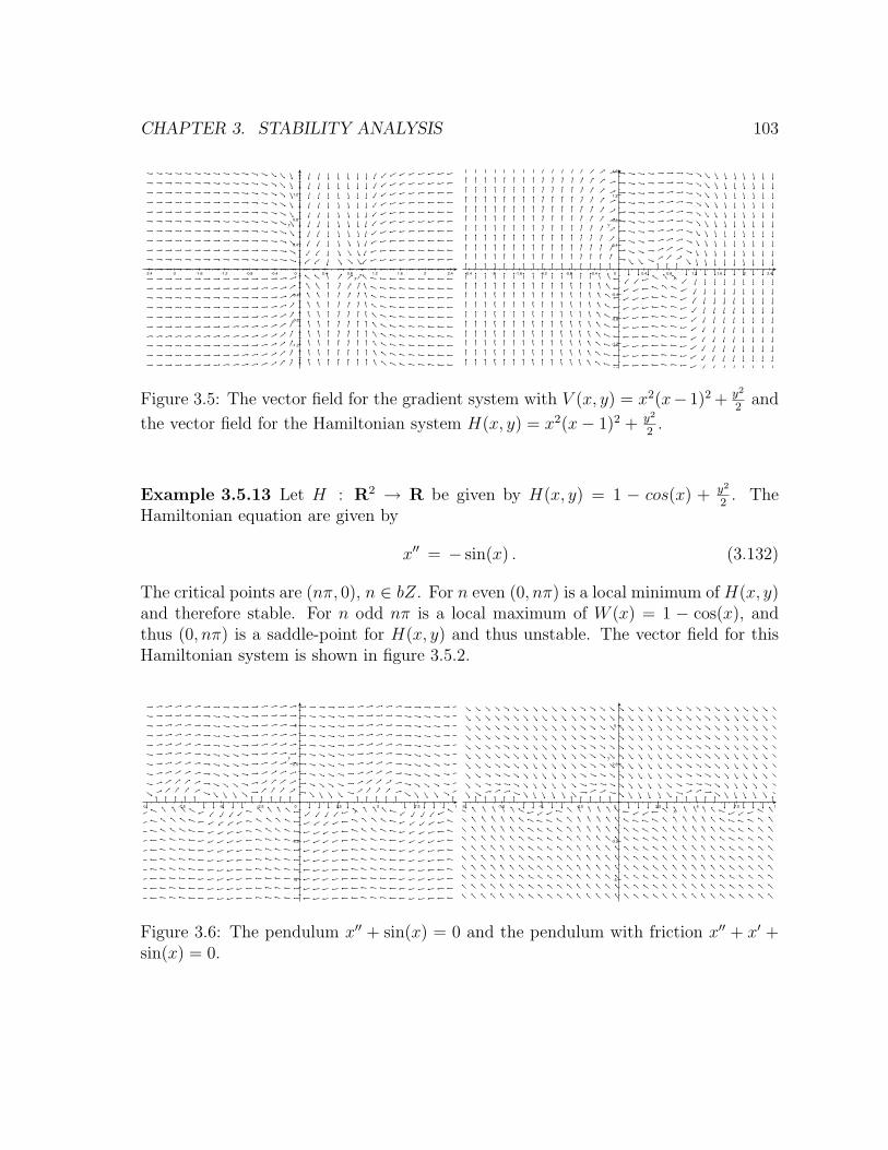
CHAPTER 3. STABILITY ANALYSIS 103
-2.4 -2 -1.6 -1.2 -0.8 -0.4 0 0.4 0.8 1.2 1.6 2 2.4
-1.2
-0.8
-0.4
0.4
0.8
1.2
-2.4 -2 -1.6 -1.2 -0.8 -0.4 0 0.4 0.8 1.2 1.6 2 2.4
-1.6
-1.2
-0.8
-0.4
0.4
0.8
1.2
1.6
Figure 3.5: The vector field for the gradient system with V (x, y) = x2(x− 1)2 + y2
2and
the vector field for the Hamiltonian system H(x, y) = x2(x− 1)2 + y2
2.
Example 3.5.13 Let H : R2 → R be given by H(x, y) = 1 − cos(x) + y2
2. The
Hamiltonian equation are given by
x′′ = − sin(x) . (3.132)
The critical points are (nπ, 0), n ∈ bZ. For n even (0, nπ) is a local minimum of H(x, y)and therefore stable. For n odd nπ is a local maximum of W (x) = 1 − cos(x), andthus (0, nπ) is a saddle-point for H(x, y) and thus unstable. The vector field for thisHamiltonian system is shown in figure 3.5.2.
-10 -7.5 -5 -2.5 0 2.5 5 7.5 10
-5
-2.5
2.5
5
-10 -7.5 -5 -2.5 0 2.5 5 7.5 10
-5
-2.5
2.5
5
Figure 3.6: The pendulum x′′ + sin(x) = 0 and the pendulum with friction x′′ + x′ +sin(x) = 0.
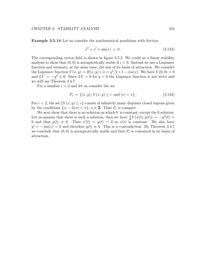
CHAPTER 3. STABILITY ANALYSIS 104
Example 3.5.14 Let us consider the mathematical pendulum with friction
x′′ + x′ + sin(x) = 0 . (3.133)
The corresponding vector field is shown in figure 3.5.2. We could us a linear stabilityanalysis to show that (0, 0) is asymptotically stable if ε > 0. Instead we use a Liapunovfunction and estimate, at the same time, the size of its basin of attraction. We considerthe Liapunov function V (x, y) = H(x, y) + 1 = y2/2 + 1− cos(x). We have V (0, 0) = 0and LV = −y2 ≤ 0. Since LV = 0 for y = 0 the Liapunov function is not strict andwe will use Theorem 3.4.7.
Fix a number c < 2 and let us consider the set
Pc = {(x, y) |V (x, y) ≤ c and |x| < π} . (3.134)
For c < 2, the set {V (x, y) ≤ c} consist of infinitely many disjoints closed regions givenby the conditions {|x− 2nπ| < π}, n ∈ Z. Thus Pc is compact.
We next show that there is no solution on which V is constant, except the 0 solution.Let us assume that there is such a solution, then we have d
dtV (x(t), y(t)) = −y2(t) =
0 and thus y(t) ≡ 0. Thus x′(t) = y(t) = 0 so x(t) is constant. We also havey′ = − sin(x) = 0 and therefore q(t) ≡ 0. This is a contradiction. By Theorem 3.4.7we conclude that (0, 0) is asymptotically stable and that Pc is contained in its basin ofattraction.
Chapter 4
Poincare-Bendixson Theorem
We discuss in this chapter the long time limit of two dimensional autonomous systems.In particular, we discuss in the problem of the existence of periodic solutions for twodimensional systems. Closed orbits correspond to periodic solutions and accordingJordan closed curve theorem they separate R2 into two connected components, theinterior of and the exterior of the orbits. This makes the 2-dimensional case specialand much more tractable then the general case.
4.1 Limit sets and attractors
Let us consider the autonomous equation x′ = f(x) where x ∈ Rn and f(x) is locallyLipschitz. We denote by γ(x0) the orbit corresponding to the solution with x(0) = x0.In particular if x(t1) = x1 then we have γ(x0) = γ(x1). We denote by γ+(x0) the positiveorbit defined by x(t), t ≥ 0 and by γ−(x0) the negative orbit defined by x(t), t ≥ 0. Wehave γ(x0) = γ+(x0) ∪ γ−(x0) and for a periodic solution we have γ+(x0) = γ−(x0).
We call a set M invariant, if x(0) ∈M implies that x(t) ∈M for all t ∈ R and wecall a set positively invariant , if x(0) ∈M implies that x(t) ∈M for all t ≥ 0.
Definition 4.1.1 A point x∗ is called a positive limit point of the orbit γ(x0) if thereexists an increasing sequence tn with limn→∞ tn =∞ such that x∗ = limn→∞ x(tn). Anegative limit point of γ(x0) is defined similarly.
Example 4.1.2 For the equation x′ = −2x and y′ = −y, for all orbits (0, 0) is theunique limit point.
Example 4.1.3 If x′ = f(x) has a periodic orbit C, every point on the periodic orbitis a positive and negative limit point of the orbit.
Definition 4.1.4 We denote by ω(γ) the set of all positive limit points for the orbitγ, it is called the ω-limit set of γ. Similarly we denote α(γ) the set of all negative limitpoints for the orbit γ (the α-limit set of γ).
CHAPTER 4. POINCARE-BENDIXSON THEOREM 106
The basic properties of limit points and limit sets are summarized in
Theorem 4.1.5 The sets ω(γ) and α(γ) are closed and invariant. If the positive orbitγ+ is bounded, then ω(γ) is a compact, connected and non-empty set. If γ+ = γ+(x0)then we have limt→∞ dist (x(t, 0, x0) , ω(γ)) = 0. Analogous properties hold for γ− andα(ω).
Proof: We first prove that ω(γ) is closed. Let {ym} be a convergent sequence in ω(γ)with limit y. We show that y is a limit point. For any ε > 0, there exists M such that,for any m ≥M , ‖ym − y‖ ≤ ε/2 and there exist sequences tmn with limn t
(m)n =∞ such
that ‖x(t(m)n )− ym‖ ≤ ε/2. This implies that y is a limit point.
We next show that ω(γ) is an invariant invariant. Let x∗ ∈ ω(γ), then there existsa sequence {tn} with tn → ∞ such that limn x(tn) = x∗. For arbitrary t, we havex(t+ tn, 0, x0) = x(t, 0, x(tn, 0, x0)) so that, using the continuous dependence on initialconditions we have limn x(t + tn, x0) = x(t, 0, x∗). Therefore for all t, the orbit whichcontains x∗ lies in ω(γ) and this proves invariance.
Let us assume that γ+ is bounded, then it has at least one accumulation point andso ω(γ) is non empty. Since ω(γ) is closed it is also compact.
Since, for any t, limn x(t+ tn, 0, x0) = x(t, x∗) we have γ(x∗) ⊂ ω(γ(x0)). It followsthat limt→∞ dist (x(t, 0, x0) , ω(γ)) = 0. This also implies that ω(γ) is connected.
Definition 4.1.6 We say that a closed invariant set A is an attracting set if there is aopen neighborhood U of A such that for all points x0 ∈ U , x(t, 0, x0) ∈ U for all t > 0and limt→∞ dist (x(t) , A) = 0. An attractor is an attracting set which contains a denseorbit. A stable limiting cycle is an attractor which consists of a single periodic orbit.
Example 4.1.7 For a critical point a, we always have γ(a) = a and so {a} contains adense orbit. If a is is asymptotically stable then it is an attractor.
Example 4.1.8 Consider the system x′ = x−x3 and y′ = −y. The system has threecritical points (−1, 0) and (1, 0) which are asymptotically stable and (0, 0) which is asaddle point. The set A = {y = 0 , −1 ≤ x ≤ 1} is an attracting set, every orbit isattracted to A. But A does not contain a dense orbit and it is not an attractor.
Example 4.1.9 Consider the system
x′ = −y + x(1− x2 − y2) ,
y′ = x+ y(1− x2 − y2) . (4.1)
It is convenient to write the equation in polar coordinates, x = r cos(θ), y = r sin(θ).A simple computation shows that (4.1) is equivalent to
r′ = r(1− r2) ,
θ′ = 1 . (4.2)
CHAPTER 4. POINCARE-BENDIXSON THEOREM 107
We see that the origin is an equilibrium point of the system. The set r = 1 is invariantand consists of a periodic orbit of period 2π. The origin is unstable and the flow spiralsoutward (counterclockwise) for 0 < r < 1 and inward for r > 1. The circle {r = 1} isa stable limiting cycle. Each point in the open neighborhood U = {a < r < A} wherea > 0 is attracted to the limiting cycle.
Example 4.1.10 Consider the system (in polar coordinates)
r′ = r(1− r) ,θ′ = sin2(θ) + (1− r)3 . (4.3)
Both the origin and the circle {r = 1} are invariant set. The circle {r = 1} is the ω-limit set for all orbits starting outside the origin and outside the circle. The invariantset {r = 1} consists of four orbits given by θ = 0, θ = π, and the arcs 0 < θ < π, andπ < θ < 2π.
4.2 Poincare maps and stability of periodic solu-
tions
We begin by considering a periodic system
x′ = f(t, x) , (4.4)
where f(t, x) is periodic of period p, f(t + p, x) = f(t, x). Let us assume that f isof class C1 and that eq. (4.4) has a periodic solution xp(t) of period p. We linearizearound the periodic solution, i.e., we set y(t) = x(t)− xp(t) so that
y′(t) =df
dx(t, p(t))y + h(t, y) , (4.5)
where
h(t, y) = f(t, y + xp(t))− f(t, xp(t))−df
dx(t, p(t))y . (4.6)
Note that h(t, y) satisfies h(t, 0) = 0 and for any t0
lim‖y‖→0
supt>t0
‖h(t, y)‖‖y‖
= 0 . (4.7)
The linearized equation is
y′(t) =df
dx(t, p(t))y , (4.8)
CHAPTER 4. POINCARE-BENDIXSON THEOREM 108
where A(t) = dfdx
(t, p(t)) is periodic of period p. By Floquet theorem, there exists aperiodic matrix P (t) and a matrix R such that the transformation y = P (t)z transformthe system into the form
z′ = Az + P−1(t)h(t, P (t)z) . (4.9)
The stability properties of the 0 solution of (4.9) are thus equivalent to the stabilityproperties of the periodic solution xp(t). From the stability/instability theorem 3.1.1and 3.1.2 we conclude that the periodic solution xp(t) is stable if all eigenvalues of Ahave negative real parts and that xp(t) is unstable if at least one eigenvalue of A haspositive real part.
This simple and appealing stability analysis however breaks down completely ifxp(t) is a periodic solution of the autonomous system
x′ = f(x) , (4.10)
where f is of class C1. In this case we have
y′(t) =df
dx(p(t))y + h(t, y) , (4.11)
where
h(t, y) = f(y + xp(t))− f(xp(t))−df
dx(p(t))y . (4.12)
and the linearized equation is
y′(t) =df
dx(p(t))y . (4.13)
As we have already noted in Section 2.5, x′p(t) is always a periodic solution of thevariational equation. This implies that R always has an eigenvalue 0 and thereforexp(t) cannot be asymptotically stable. This can be also seen as follows: since f doesnot depend on x, if xp(t) is a periodic solution, then yp(t) = xp(t+δt) is also a periodicsolution. For small δt, yp(t) is near xp(t) at t = 0 but |yp(t)− xp(t)| does not tend to0 as t→∞.
For periodic solutions a much more natural concept of stability is to require thatthat if C is the periodic orbit corresponding to xp(t) there exists δ > 0 such that if‖xp(0)− x(0)‖ ≤ δ then
limt→∞
dist(x(t), C) = 0 . (4.14)
If, in addition, there exists a number α ∈ [0, p) such that limt→∞ ‖x(t)−xp(t+α)‖ = 0,then x(t) is said to have asymptotic phase α. This means that the solution x(t) windsaround as it approaches the periodic solution xp(t).
CHAPTER 4. POINCARE-BENDIXSON THEOREM 109
We also introduce the concept of the Poincare map. Let C be a periodic orbit ofthe autonomous system
x′ = f(x) , (4.15)
corresponding to the a periodic solution xp(t). Let us assume that the orbit passespasses through the point x0. Let Ξ be an hyperplane perpendicular to the orbit C atx0. If x ∈ Ξ is sufficiently close to x0, then the solution starting at x at t = 0 will crossthe hyperplane Ξ at a point P (x) near x0. The mapping x 7→ P (x) is called a Poincaremap.
There is nothing special about hyperplanes and so the Poincare map can be definedin a similar way if Ξ is a smooth hypersurface through x0 which is not tangent to theperiodic orbit C.
Theorem 4.2.1 Let f : U → Rn (U an open set of Rn) be of class C1 and letφt(x) denote the flow defined by the differential equation x′ = f(x). Assume thatxt(p) = φt(x0) is a periodic solution of period p and the orbit {φt(x0)}0≤t≤p is containedin U . Let Ξ be the hyperplane orthogonal to C at x0, i.e.
Ξ = {x ∈ Rn , 〈(x− x0) , f(x0)〉 = 0} . (4.16)
Then there exists δ > 0 and a unique function τ(x) which is defined and continuouslydifferentiable in Nδ(x0) = {x ∈ Ξ ; ‖x− x0‖ < δ} so that τ(x0) = p and
φτ(x)(x) ∈ Ξ , for all x ∈ Nδ(x0) . (4.17)
Proof: This is an consequence of the smooth dependence of φt(x) with respect to x andt (see Theorem 2.6.6) and from the implicit function theorem. We define the function
F (t, x) =⟨(φt(x)− x0) , f(x0)
⟩. (4.18)
The function F (t, x) is of class C1 for (t, x) ∈ R× U . Since φp(x0) = x0 we have
F (p, x0) = 0 . (4.19)
Since ∂φt(x0)∂t|t=p = f(x0) we have
∂F
∂t(p, x0) =
⟨∂φt(x0)
∂t|t=p , f(x0)
⟩= 〈f(x0) , f(x0)〉 6= 0 , (4.20)
since x0 is not a critical point. From the implicit function theorem there exists afunction τ(x) of class C1 defined in a neighborhood Bδ(x0) such that τ(x0) = x0 and
F (τ(x), x) =⟨(φτ(x)(x)− x0) , f(x0)
⟩= 0 , (4.21)
CHAPTER 4. POINCARE-BENDIXSON THEOREM 110
i.e.,φτ(x)(x) ∈ Ξ . (4.22)
This concludes the proof by taking Nδ(x0) = Bδ(x0) ∩ Ξ.
Theorem 4.2.1 implies that the Poincare map P : Nδ(x0)→ Ξ given by
P (x) = φτ(x)(x) , (4.23)
is well defined and of class C1. Fixed points of the Poincare map P (x) = x correspondto periodic orbits φt(x) for (4.15). One can also show easily that the map P (x) isinvertible with an inverse of class C1 given P−1(x) = φ−τ(x)(x).
Example 4.2.2 For the system
x′ = −y + x(1− x2 − y2) ,
y′ = x+ y(1− x2 − y2) . (4.24)
or equivalently, in polar coordinates
r′ = r(1− r2) ,
θ′ = 1 . (4.25)
we can compute the Poincare map explicitly. The solution to equations (4.25) withr(0) = r0 and θ(0) = θ0 are
r(t, r0) =
[1 +
(1
r20
− 1
)e−2t
]− 12
,
θ(t, θ0) = t+ θ0 . (4.26)
Let Ξ be the ray θ = θ0 through the origin, then Ξ is perpendicular to the closed orbitr = 1. Any trajectory starting at (r0, θ0) at time 0 intersects Ξ at time 2π. Thereforethe Poincare map is given by
P (r0) =
[1 +
(1
r20
− 1
)e−4π
]− 12
. (4.27)
with P (1) = 1 and
P ′(r0) = e−4π 1
r30
[1 +
(1
r20
− 1
)e−4π
]− 32
(4.28)
so that P ′(1) = e−4π < 1.
CHAPTER 4. POINCARE-BENDIXSON THEOREM 111
For two-dimensional system, Ξ is a line segment intersecting C orthogonally. Wecan parametrize the line Ξ by the distance s to the intersection point x0. We canthen write the Poincare map as P = P (s) as a a function of s which is defined in aneighborhood of the origin and satisfy P (0) = 0.
The stability of the periodic orbit C is determined by P ′(0). To see this let usintroduce the displacement function
d(s) = P (s)− s . (4.29)
Then d(0) = 0 and d′(s) = P ′(s)− 1. If d′(0) 6= 0 then, by continuity the sign of d(s)will be the same in a neighborhood of 0. Thus if d′(0) < 0 (i.e P ′(0) < 1) thereforethe periodic orbit C is a stable limit cycle since the successive intersection of the orbitwith Ξ approach 0. Similarly if d′(0) < 0 (i.e., P ′(0) < 1) C is an unstable limit cycle.
Example 4.2.3 For the example 4.2.2 we have seen that P ′(1) < 1 which means thatthe circle r = 1 is a stable limit cycle.
This analysis can be generalized easily to higher dimension. Suppose P that thePoincare P : Nδ(x0) → Ξ satisfies P (x0) = x0 and that the n − 1 eigenvalues ofthe derivative P ′(x0) at x0 have all absolute value less than 1. Since the map Pis differentiable, P ′(x) is continuous and therefore for x sufficiently close to x0 allthe eigenvalues of P ′(x) have also absolute values less than 1. This implies that thesuccessive approximation of the orbits with Ξ approach 0.
It turns out that the eigenvalues of P ′(0) are closely related to the Floquet multi-pliers of the linearization around the periodic orbit xp(t).
Theorem 4.2.4 Let f : U → Rn (U ⊂ Rn open) be of class C1 and let assume thatxp(t) is periodic orbit for x′ = f(x) which is contained in U . For δ sufficiently smalllet P (x) : Nδ(x0) → Ξ be the Poincare map for xp(t). Let λ1, · · · , λn−1 be the n − 1eigenvalues of P ′(0) then λ1, · · · , λn−1, 1 are the Floquet multipliers for the linearizedequation
x′ = A(t)x , A(t) =df
dx(xp(t)) . (4.30)
Proof: Without restricting generality, by a change of variable, we can assume thatx0 = 0 and that f(0) = (0, · · · , 0, 1)T . This means that the hyperplane Ξ is thehyperplane xn = 0.
The flow for x′ = f(x) is denoted by φt(x) and H(t, x) ≡ ∂∂xφt(x) satisfies the
variational equation
∂
∂tH(t, x) =
df
dx(φt(x))H(t, x) , H(0, x) = I (4.31)
CHAPTER 4. POINCARE-BENDIXSON THEOREM 112
In particular for x = 0, H(t, 0) is the resolvent for (4.30). Since xp(t) is a solutionof x′ = f(x) then x′p(t) is a solution of (4.30) with initial condition x′p(0) = f(0). Fort = p, x′p(p) = f(0) and thus
H(t, 0)f(0) = f(0) , (4.32)
i.e., 1 is an eigenvalue of H(p, 0) with eigenvector f(0). By Floquet Theorem H(p, 0) =C = epR and thus 1 is a Floquet multiplier with eigenvector f(0) = (0, · · · , 0, 1)T .Therefore the last column of H(p, 0) is the vector (0, · · · , 0, 1)T .
Recall that the Poincare map P (x) is defined to be the restriction to Ξ of the maph(x) where H is given by
h(x) = φτ(x)(x) (4.33)
and τ(x) is the first time the solution hits the hyperplane Ξ (see Theorem 4.2.1). Wehave
dh
dx(x) =
∂
∂tφτ(x)(x)
dτ
dx(x) +
∂
∂xφτ(x)(x)
=∂
∂tφτ(x)(x)
dτ
dx(x) +H(τ(x), x) , (4.34)
and thus for x = 0 we obtain
dh
dx(0) = f(0)
dτ
dx(0) +H(p, 0) ,
=
0 · · · 0 0...
. . ....
...0 · · · 0 0
∂τ∂x1
(0) · · · · · · ∂τ∂xn
(0)
+
0
H(p, 0)...0
· · · 1
(4.35)
By our choice of coordinates the derivative of P (x) consists of the first n− 1 rows andcolumns of dh
dxand therefore
dP
dx(0) = H(p, 0) . (4.36)
where H(p, 0) is the matrix consisting of the first n − 1 rows and columns of H(p, 0).
Remark 4.2.5 It is in general very difficult to compute the Poincare map explicitly,and as the previous theorem shows, it is also very difficult to compute the derivative ofthe Poincare map since it amounts to computing the Floquet multipliers for a systemwith periodic periodic coefficients. The concept of the Poincare map is however veryuseful, it plays for example a central role int the Poincare-Bendixson theorem on theexistence of periodic orbits for planar systems.
CHAPTER 4. POINCARE-BENDIXSON THEOREM 113
4.3 Bendixson criterion
We consider the autonomous system
x′ = f(x) (4.37)
where f is of class C1 in an open set U ⊂ R2. We derive a simple sufficient conditioncriterion for a two dimensional not to have a periodic orbit.
Theorem 4.3.1 (Bendixson criterion) Suppose that the open D ⊂ R2 is simplyconnected and f is of class C1. The equation (4.37) can have a periodic solution onlyif div f changes sign in D or div f = 0 in D.
Proof: Suppose that we have a closed orbit C in D and let G be the interior of theorbit C. By the divergence theorem (Gauss Theorem) we have,∫ ∫
Gdivf dx =
∫Cf ·ds =
∫C
(f1dx2−f2dx1) =∫C
(f1dx2
dt− f2
dx1
dt
)dt = 0 (4.38)
where the last equality follows from the fact that the closed curve C can be parametrizedby a solution of (4.37). So the integral on the left side vanishes which implies that div feither vanishes or changes sign in D.
Example 4.3.2 The Lienard equation is given x′′+f(x)x′+g(x) = 0 where f(x) andg(x) are Lipschitz continuous. The vector fields h(x, y) = (y,−f(x)y− g(x))T satisfiesdiv f(x, y) = −f(x). If f(x) is either positive or negative then Theorem (4.3.1) impliesthat there is no periodic solution.
Example 4.3.3 For the van der Pol equation x′′ + ε(x2 − 1)x′ + x = 0 we havediv f(x, y) = −ε(x2 − 1). So a periodic solution, if it exists, must intersect with thelines x = 1 or x = −1.
4.4 Poincare-Bendixson Theorem
In this section we prove
Theorem 4.4.1 Let f : U → R2 (U an open set of R2) be of class C1. Assume thatthe positive orbit γ+ for the system
x′ = f(x) , (4.39)
is bounded and that the limit set ω(γ+) does not contain critical points. Then ω(γ+) isa periodic orbit.
CHAPTER 4. POINCARE-BENDIXSON THEOREM 114
We will split the proof of the theorem in a sequence of lemmas. We first introducethe concept of a transversal line and regular points for (4.39).
Definition 4.4.2 A finite closed segment of a straight line l contained in U is transver-sal for (4.39) if l does not contain any critical points of (4.39) and if the vector field fis not tangent to l at any point of l.
Definition 4.4.3 A point x ∈ U is regular for (4.39) if it is not a critical point for(4.39).
Lemma 4.4.4 Let x∗ be an interior point of a transversal l, then for any ε > 0, thereexists δ > 0 such that every trajectory passing through a point x with ‖x − x∗‖ ≤ δcrosses l at some time t with |t| ≤ ε.
Proof: This follows from the continuity of the vector field f . Since l contains onlyregular points, the vector field on l always points on the same side of l. A sufficientlysmall neighborhood of l contains also only regular points. This implies that an orbitstarting close enough from l will actually crosses it for some positive or negative time.The lemma follows then by the continuous dependence of the solution from initialconditions.
Lemma 4.4.5 1. If a finite closed arc {x(t) : a ≤ t ≤ b} of a trajectory γ intersectsa transversal l, it does so at a finite number of points.
2. If γ is a periodic orbit which intersects l, it does intersect l only once.
3. The successive intersections with l form a monotonic sequence (with respect tothe order on the line l).
Proof: Let us assume that for t ∈ [a, b], x(t) intersects the transversal at infinitely manypoints xn = x(tn). Then the sequence tn will have an accumulation point t∗ ∈ [a, b].Passing to a subsequence, also denoted by {tn} we have that x(tn) converges to x(t∗)in l. But on the other hand we have
limn→∞
x(tn)− x(t∗)
tn − t∗= x′(t∗) = f(x(t∗)) . (4.40)
which is a vector tangent to l at x(t∗). Since x(tn), x(t∗) ∈ l this is a contradiction tothe fact that l is transversal. This proves 1 and thus a fine segment of an orbit meetsl finitely many times.
Let now x1 = x(t1) and x2 = x(t2) with t1 < t2 be two successive point of in-tersection of the orbit with l. Suppose that x1 is distinct from x2. Then the arc{x(t) : t1 ≤ t ≤ t2} together with the closed segment x1x2 on l forms a closed Jordan
CHAPTER 4. POINCARE-BENDIXSON THEOREM 115
curve J . By Jordan closed curve Theorem J separates the plane into two regions, theinterior of J and the exterior of J . The points x(t) with t < t1 (and t close to t1) andthe points x(t) with t > t2 (and t close to t2) will be on the opposite sides of the curveJ . It, in fact, remains so for all times t < t1 and t > t2. Suppose for example x(t),t > t2 is inside J . The orbit cannot cross J on the transversal because the flow pointsinward on the transversal, it cannot cross either on the orbit part of J by uniquenessof solutions. Therefore x(t) must remains inside J for all t > t2. A similar argumentholds if x(t), t < t1 is inside J .
From this 2 and 3 follows immediately.
This lemma gives some insight in the structure of possible ω-limit sets in R2.
Lemma 4.4.6 If an orbit γ and its ω-limit set ω(γ) have a point in common, then γis either a critical point or a periodic orbit.
Proof: Let x1 = x(t1) ∈ γ ∩ ω(γ). If x1 is a critical point then x(t) = x1 for all t ∈ R.If x1 is a regular point, then we can find a transversal l such that x1 is an interior pointof l. Since x1 ∈ ω(γ), there exists a point x∗ = x(t∗) with, say, t∗ > t1 + 2 which is atdistance no more than δ from x1. By lemma (4.4.4) the orbits passing through x∗ willintersect l at a time t2 > t1 + 1. If x2 = x1 then ω(γ) is periodic orbit. If x2 6= x1, thenthe piece of orbit {x(t) ; t1 ≤ t ≤ t2} intersect l only at a finite number of points, bylemma 4.4.5, item 1. By Lemma 1, item 3, the successive intersections of γ with l area monotone sequence which tend away from x1. This contradicts our assumption thatx1 ∈ ω(γ).
Lemma 4.4.7 If the ω-limit set ω(γ) of an orbit γ intersect a transversal l, it doesso in one point only. If x∗ is such an intersection point, we have ω(γ) = γ with γa periodic orbit or there exists a sequence tn with limn tn = ∞ and x(tn) tends to x∗
monotonically on l.
Proof: Suppose that ω(γ) intersects l in x∗. If the orbits γ passes through x∗ then γand γ(ω) have x∗ in common which is regular point. Thus, by lemma 4.4.6 ω(γ) is aperiodic orbit. If not, x∗ being in the ω-limit set, there exists a sequence {t′n} withlimn t
′n =∞ such that limn x(t′n) = x∗. Then, by Lemma 4.4.4, there exists a sequence
tn with limn tn = ∞ such that x(tn) ∈ l and limn x(tn) = x∗ monotonically in l byLemma 4.4.5.
Now suppose that there exists another intersection point y∗ of ω(γ) with l. By thesame argument we can construct a sequence x(sn) which tends monotonically in l toy∗. But in that case we can construct a sequence of intersection of the orbit with lwhich is not monotone. This contradicts Lemma 4.4.5.
CHAPTER 4. POINCARE-BENDIXSON THEOREM 116
Lemma 4.4.8 If ω(γ) contains no critical point and ω(γ) contains a periodic orbit C,then ω(γ) = C.
Proof: Let us suppose ω(γ) \C is not empty. Since ω(γ) is connected, C must containa limit point x∗ of the set ω(γ) \ C. Let l be a transversal which contains x∗, fromlemma 4.4.7 it follows that that ω(γ) intersects l only at x∗. Since x∗ is a limit pointof ω(γ) \ C, then there exist a point y of ω(γ) \ C in arbitrarily small neighborhoodsof x∗. By Lemma 4.4.4 an orbit through y will intersect l, since y ∈ ω(γ) and ω(γ) isan invariant set, an orbit through y belongs also to ω(γ) and this contradicts lemma4.4.7.
With these preparations we can now conclude the proof of Theorem 4.4.1.
Proof of Theorem 4.4.1: Since γ+ is bounded, ω(γ+) is compact, connected and notempty. If γ+ is a periodic orbit then, by lemma 4.4.8, γ+ = ω(γ+). Suppose γ+ 6=ω(γ+). There exists an orbit C ⊂ ω(γ+) and the orbit C is contained in compactbounded set F . Therefore the orbit C has itself a limit point x∗ which is in ω(γ+) sinceω(γ+) is closed. Let l be a transversal through x∗, then by Lemma 4.4.7, l intersectsω(γ+) only at x∗. Since x∗ is a limit point of C, by Lemma (4.4.4), l must also intersectsC at some point which must be then x∗. This implies that C and ω(C) have a pointin common and so, by lemma 4.4.6, C must be a periodic orbit. By lemma 4.4.8 thisimplies that ω(γ+) = C.
We can derive several consequences from Theorem (4.4.1). If ω(γ) is a periodicorbit C, we call it a ω-limit cycle. We have seen that dist(x(t), ω(γ)) → 0 as t → ∞,which means that the orbit spirals toward C.
Limit cycles possess a kind of (at least one-sided) stability.
Corollary 4.4.9 Let C be an ω-limit cycle. If C = ω(γ(x)), then there exists a neigh-borhood O of x such that C = ω(γ(y)) for all y ∈ O. The set
{y |ω(γ(y)) = C} \ γ (4.41)
is an open set.
Proof: Let l be a transversal to C. Then there exists a line segment f in l, which isdisjoint from C and is bounded by x(t1) and x(t2) with t1 < t2 and such that x(t)does not meet this segment for t1 < t < t2. Consider now the region A bounded oneside by C and on the other side by the closed curve consisting of the orbit segment{x(t)t1 ≤ t ≤ t2} and the line segment f . This region is positively invariant and ify ∈ A \ γ the orbit passing through y spirals toward C.
If there exists orbits attracted to C starting on both sides of C, then C is anattractor.
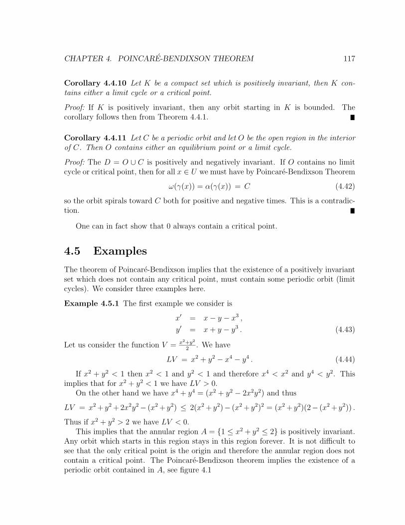
CHAPTER 4. POINCARE-BENDIXSON THEOREM 117
Corollary 4.4.10 Let K be a compact set which is positively invariant, then K con-tains either a limit cycle or a critical point.
Proof: If K is positively invariant, then any orbit starting in K is bounded. Thecorollary follows then from Theorem 4.4.1.
Corollary 4.4.11 Let C be a periodic orbit and let O be the open region in the interiorof C. Then O contains either an equilibrium point or a limit cycle.
Proof: The D = O ∪ C is positively and negatively invariant. If O contains no limitcycle or critical point, then for all x ∈ U we must have by Poincare-Bendixson Theorem
ω(γ(x)) = α(γ(x)) = C (4.42)
so the orbit spirals toward C both for positive and negative times. This is a contradic-tion.
One can in fact show that 0 always contain a critical point.
4.5 Examples
The theorem of Poincare-Bendixson implies that the existence of a positively invariantset which does not contain any critical point, must contain some periodic orbit (limitcycles). We consider three examples here.
Example 4.5.1 The first example we consider is
x′ = x− y − x3 ,
y′ = x+ y − y3 . (4.43)
Let us consider the function V = x2+y2
2. We have
LV = x2 + y2 − x4 − y4 . (4.44)
If x2 + y2 < 1 then x2 < 1 and y2 < 1 and therefore x4 < x2 and y4 < y2. Thisimplies that for x2 + y2 < 1 we have LV > 0.
On the other hand we have x4 + y4 = (x2 + y2 − 2x2y2) and thus
LV = x2 + y2 + 2x2y2− (x2 + y2) ≤ 2(x2 + y2)− (x2 + y2)2 = (x2 + y2)(2− (x2 + y2)) .
Thus if x2 + y2 > 2 we have LV < 0.This implies that the annular region A = {1 ≤ x2 + y2 ≤ 2} is positively invariant.
Any orbit which starts in this region stays in this region forever. It is not difficult tosee that the only critical point is the origin and therefore the annular region does notcontain a critical point. The Poincare-Bendixson theorem implies the existence of aperiodic orbit contained in A, see figure 4.1
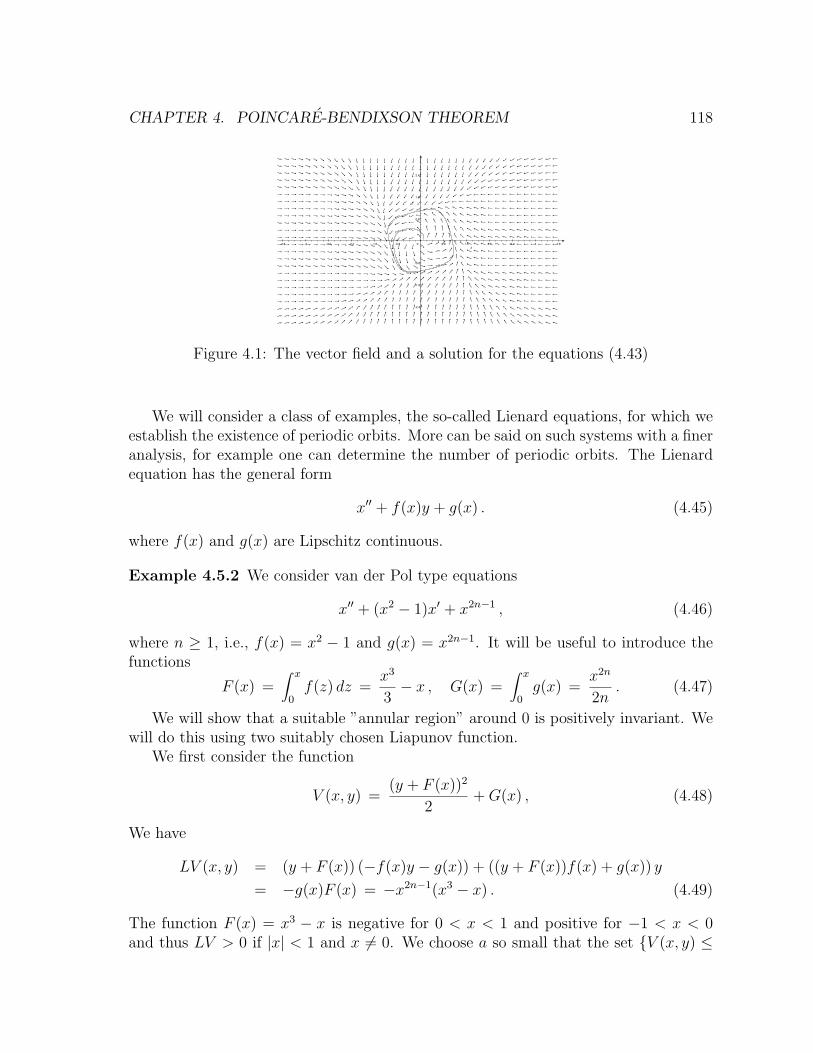
CHAPTER 4. POINCARE-BENDIXSON THEOREM 118
-4.8 -4 -3.2 -2.4 -1.6 -0.8 0 0.8 1.6 2.4 3.2 4 4.8
-2.4
-1.6
-0.8
0.8
1.6
2.4
Figure 4.1: The vector field and a solution for the equations (4.43)
We will consider a class of examples, the so-called Lienard equations, for which weestablish the existence of periodic orbits. More can be said on such systems with a fineranalysis, for example one can determine the number of periodic orbits. The Lienardequation has the general form
x′′ + f(x)y + g(x) . (4.45)
where f(x) and g(x) are Lipschitz continuous.
Example 4.5.2 We consider van der Pol type equations
x′′ + (x2 − 1)x′ + x2n−1 , (4.46)
where n ≥ 1, i.e., f(x) = x2 − 1 and g(x) = x2n−1. It will be useful to introduce thefunctions
F (x) =∫ x
0f(z) dz =
x3
3− x , G(x) =
∫ x
0g(x) =
x2n
2n. (4.47)
We will show that a suitable ”annular region” around 0 is positively invariant. Wewill do this using two suitably chosen Liapunov function.
We first consider the function
V (x, y) =(y + F (x))2
2+G(x) , (4.48)
We have
LV (x, y) = (y + F (x)) (−f(x)y − g(x)) + ((y + F (x))f(x) + g(x)) y
= −g(x)F (x) = −x2n−1(x3 − x) . (4.49)
The function F (x) = x3 − x is negative for 0 < x < 1 and positive for −1 < x < 0and thus LV > 0 if |x| < 1 and x 6= 0. We choose a so small that the set {V (x, y) ≤
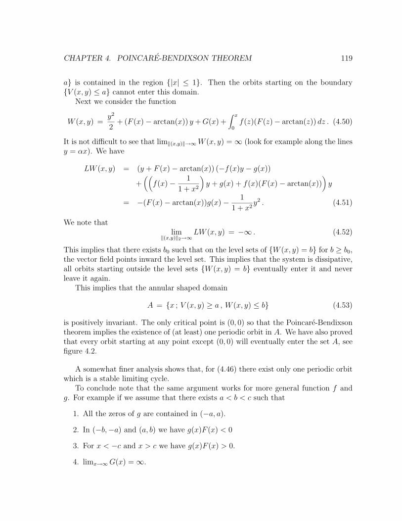
CHAPTER 4. POINCARE-BENDIXSON THEOREM 119
a} is contained in the region {|x| ≤ 1}. Then the orbits starting on the boundary{V (x, y) ≤ a} cannot enter this domain.
Next we consider the function
W (x, y) =y2
2+ (F (x)− arctan(x)) y +G(x) +
∫ x
0f(z)(F (z)− arctan(z)) dz . (4.50)
It is not difficult to see that lim‖(x,y)‖→∞W (x, y) =∞ (look for example along the linesy = αx). We have
LW (x, y) = (y + F (x)− arctan(x)) (−f(x)y − g(x))
+((f(x)− 1
1 + x2
)y + g(x) + f(x)(F (x)− arctan(x))
)y
= −(F (x)− arctan(x))g(x)− 1
1 + x2y2 . (4.51)
We note thatlim
‖(x,y)‖2→∞LW (x, y) = −∞ . (4.52)
This implies that there exists b0 such that on the level sets of {W (x, y) = b} for b ≥ b0,the vector field points inward the level set. This implies that the system is dissipative,all orbits starting outside the level sets {W (x, y) = b} eventually enter it and neverleave it again.
This implies that the annular shaped domain
A = {x ; V (x, y) ≥ a , W (x, y) ≤ b} (4.53)
is positively invariant. The only critical point is (0, 0) so that the Poincare-Bendixsontheorem implies the existence of (at least) one periodic orbit in A. We have also provedthat every orbit starting at any point except (0, 0) will eventually enter the set A, seefigure 4.2.
A somewhat finer analysis shows that, for (4.46) there exist only one periodic orbitwhich is a stable limiting cycle.
To conclude note that the same argument works for more general function f andg. For example if we assume that there exists a < b < c such that
1. All the zeros of g are contained in (−a, a).
2. In (−b,−a) and (a, b) we have g(x)F (x) < 0
3. For x < −c and x > c we have g(x)F (x) > 0.
4. limx→∞G(x) =∞.
CHAPTER 4. POINCARE-BENDIXSON THEOREM 120
-10 -7.5 -5 -2.5 0 2.5 5 7.5 10
-5
-2.5
2.5
5
Figure 4.2: The vector field and a solution for the equations (4.46) with n = 2
5. For large x, F (x) = x2n+1 + lower order terms.
then we have the existence of a periodic orbit. The number of periodic orbits dependson the detailed behavior of F , in particular how many times it changes signs betweenb and c.
Finally we consider an equation which models chemical reactions involved in thebreaking down of sugar in cells.
Example 4.5.3 Let us consider the equations
x′ = −x+ ay + x2y = f(x, y) ,
y′ = b− ay − x2y = g(x, y) , (4.54)
where a and b are positive constants.
y=b/(a+x^2)
y=x/(a+x^2)
(b , b/a)
Figure 4.3: The curves y = x/(a+ x2) y = b/(a+ x2) and the region A.
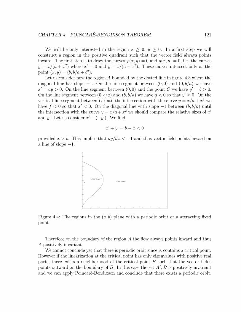
CHAPTER 4. POINCARE-BENDIXSON THEOREM 121
We will be only interested in the region x ≥ 0, y ≥ 0. In a first step we willconstruct a region in the positive quadrant such that the vector field always pointsinward. The first step is to draw the curves f(x, y) = 0 and g(x, y) = 0, i.e. the curvesy = x/(a + x2) where x′ = 0 and y = b/(a + x2). These curves intersect only at thepoint (x, y) = (b, b/a+ b2).
Let us consider now the region A bounded by the dotted line in figure 4.3 where thediagonal line has slope −1. On the line segment between (0, 0) and (0, b/a) we havex′ = ay > 0. On the line segment between (0, 0) and the point C we have y′ = b > 0.On the line segment between (0, b/a) and (b, b/a) we have g < 0 so that y′ < 0. On thevertical line segment between C until the intersection with the curve y = x/a+ x2 wehave f < 0 so that x′ < 0. On the diagonal line with slope −1 between (b, b/a) untilthe intersection with the curve y = x/a+ x2 we should compare the relative sizes of x′
and y′. Let us consider x′ − (−y′). We find
x′ + y′ = b− x < 0
provided x > b. This implies that dy/dx < −1 and thus vector field points inward ona line of slope −1.
0 0.05 0.1 0.15 0.2 0.25 0.3 0.35 0.4 0.45 0.5
0.1
0.2
0.3
0.4
0.5
0.6
0.7
0.8
0.9
1
1.1
1.2
bT>0 stable fixed point
T<0 unstable fixed point and stable limit cycle
b
aa
Figure 4.4: The regions in the (a, b) plane with a periodic orbit or a attracting fixedpoint
Therefore on the boundary of the region A the flow always points inward and thusA positively invariant.
We cannot conclude yet that there is periodic orbit since A contains a critical point.However if the linearization at the critical point has only eigenvalues with positive realparts, there exists a neighborhood of the critical point B such that the vector fieldspoints outward on the boundary of B. In this case the set A \B is positively invariantand we can apply Poincare-Bendixson and conclude that there exists a periodic orbit.
CHAPTER 4. POINCARE-BENDIXSON THEOREM 122
We havedf
dx=
(−1 + 2xy a+ x2
−2xy −(a+ x2)
). (4.55)
and the critical point is (b, b/(a+ b2)).Note that the determinant is (a + x2) which is always positive. The trace at the
critical point is given by
τ = −b4 + (2a− 1)b2 + (a+ a2)
a+ b2(4.56)
So the fixed point has two eigenvalues with negative real parts if τ > 0. The curveτ = 0, see figure 4.3, is given by
b2 =1
2
(1− 2a±
√1− 8a
)(4.57)
and divide the positive quadrant in the (a, b)-plane into two regions: one with a stablelimit cycle and the other with a stable fixed point.
Bibliography
[1] Arnold, Vladimir I. Ordinary differential equations. Translated from the thirdRussian edition. Springer Textbook. Springer-Verlag, Berlin, 1992.
[2] Arnold, Vladimir I. Mathematical methods of classical mechanics. Second edi-tion. Graduate Texts in Mathematics, 60. Springer-Verlag, New York, 1989.
[3] Nohel, John A.; Brauer, Fred; Vleck, F. S. Van; Reviews: Qualitative Theoryof Ordinary Differential Equations. An Introduction. Reprint of 1969 edition.Dover Publications, Inc., New York 1989.
[4] Chicone, Carmen Ordinary differential equations with applications. Texts inApplied Mathematics, 34. Springer-Verlag, New York, 1999.
[5] Coddington, Earl A. and Levinson, Norman Theory of ordinary differen-tial equations. McGraw-Hill Book Company, Inc., New York-Toronto-London,1955.
[6] Hairer, Ernst .; Nrsett, Syvert, and Wanner, Gerhard. Solving ordinary dif-ferential equations. I. Nonstiff problems. Second edition. Springer Series inComputational Mathematics, 8. Springer-Verlag, Berlin, 1993.
[7] Hairer, Ernst and Wanner, Gerhard. Solving ordinary differential equations.II. Stiff and differential-algebraic problems. Second edition. Springer Series inComputational Mathematics, 14. Springer-Verlag, Berlin, 1996.
[8] Hartman, Philip Ordinary differential equations. Corrected reprint of the sec-ond (1982) edition. Classics in Applied Mathematics, 38. Society for Industrialand Applied Mathematics (SIAM), Philadelphia, PA, 2002.
[9] Hirsch, Morris W., Smale, Stephen, and Devaney, Robert L. Differential equa-tions, dynamical systems, and an introduction to chaos. Second edition. Pureand Applied Mathematics (Amsterdam), 60. Elsevier/Academic Press, Ams-terdam, 2004.
123
BIBLIOGRAPHY 124
[10] Hurewicz, Witold Lectures on ordinary differential equations. Reprint of the1964 edition. Dover Publications, Inc., New York, 1990.
[11] Miller, Richard K.; Michel, Anthony N. Ordinary differential equations. Aca-demic Press, Inc. [Harcourt Brace Jovanovich, Publishers], New York-London,1982.
[12] Perko, Lawrence Differential equations and dynamical systems. Third edition.Texts in Applied Mathematics, 7. Springer-Verlag, New York, 2001.
[13] Strogatz, Steven H. Nonlinear Dynamics and Chaos: With Applications toPhysics, Biology, Chemistry and Engineering. Studies in Nonlinearity. PerseusBooks Group, 1994.
[14] Verhulst, Ferdinand Nonlinear differential equations and dynamical systems.Second edition. Universitext. Springer-Verlag, Berlin, 1996.
[15] Walter, Wolfgang Ordinary differential equations. Graduate Texts in Mathe-matics, 182. Readings in Mathematics. Springer-Verlag, New York, 1998.