DHS SPATIAL ANALYSISREPORTS 9

SPATIAL INTERPOLATION WITH DEMOGRAPHIC AND HEALTH SURVEY DATA: KEY CONSIDERATIONS

SEPTEMBER 2014

This publication was produced for review by the United States Agency for International Development (USAID). The report was prepared by Clara Burgert et al. of ICF International, Rockville, MD, USA.

DHS Spatial Analysis Reports No. 9

Spatial Interpolation with Demographic and Health Survey Data:

Key Considerations

DHS Spatial Interpolation Working Group

ICF International

Rockville, Maryland, USA

September 2014

Corresponding author: Clara R. Burgert, International Health and Development, ICF International, 530 Gaither Road, Suite 500, Rockville, Maryland, USA; phone: 301-572-0446; e-mail: clara.burgert@icfi.com

Editors: Sidney Moore Document Production: Yuan Cheng

This study was carried out with support provided by the United States Agency for International Development (USAID) through The DHS Program (#GPO–C–00–08–00008–00). The views expressed are those of the authors and do not necessarily reflect the views of USAID or the United States Government.

The DHS Program assists countries worldwide in the collection and use of data to monitor and evaluate population, health, and nutrition programs. For additional information about The DHS Program contact: DHS Program, ICF International, 530 Gaither Road, Suite 500, Rockville, MD 20850, USA. Phone: 301-407-6500; Fax: 301-407-6501; Email: reports@dhsprogram.com; Internet: www.dhsprogram.com.

Recommended citation:

DHS Spatial Interpolation Working Group. 2014. Spatial Interpolation with Demographic and Health Survey Data: Key Considerations. DHS Spatial Analysis Reports No. 9. Rockville, Maryland, USA: ICF International.

iii

Contents

Tables ........................................................................................................................................................... v

Figures .......................................................................................................................................................... v

Boxes ............................................................................................................................................................ v

Abbreviations ............................................................................................................................................. vi

Preface ........................................................................................................................................................ vii

Abstract ....................................................................................................................................................... ix

Executive Summary ................................................................................................................................... xi

1. Introduction ............................................................................................................................................. 1

1.1. Background .................................................................................................................................... 1

1.2. Literature Review .......................................................................................................................... 3

1.3. Demographic and Health Surveys ................................................................................................. 4

1.4. DHS Spatial Interpolation Working Group Meeting ..................................................................... 5

2. Summary of Major Issues for Consideration ....................................................................................... 7

2.1. Data Considerations ...................................................................................................................... 7

2.2. Method Considerations ............................................................................................................... 11

3. Conclusion and Recommendations ...................................................................................................... 17

References .................................................................................................................................................. 19

Appendix A ................................................................................................................................................ 21

Appendix B ................................................................................................................................................ 22

Appendix C ................................................................................................................................................ 23

v

Tables

Table 1. Spatial modelling techniques applied in studies using DHS GPS data for spatial modelling and interpolation, publications 2001-2012 ..................................................................................... 4

Table 2. Appropriateness of DHS indicators for spatial interpolation .......................................................... 8

Table 3. Essential and desirable guidelines for spatial interpolation summarized by method ................... 13

Figures

Figure 1. Pepfar example (Heard and Fellenz 2012) – Ethiopia: three ways of looking at HIV distribution .................................................................................................................................... 2

Figure 2. Example of interpolated data (Gosoniu et al. 2012) ..................................................................... 3

Figure 3. Decision tree for selecting spatial interpolation methods for DHS geographic data .................. 15

Boxes

Box 1. Proposed guidelines for selection of indicators for spatial interpolation ......................................... 7

Box 2. Proposed guidelines for method selection for DHS spatial interpolation ...................................... 12

vi

Abbreviations

AIS AIDS Indicator Survey

ANC Antenatal care

DHS Demographic and Health Surveys

EA Enumeration Area

HIV Human Immunodeficiency Virus

GADM Global Administrative Areas

GIS Geographic Information System

GLM Generalized Linear Model

GPS Global Positioning System

IDW Inverse Distance Weighting

INLA Integrated Nested Laplace Approximations

MCMC Markov Chain Monte Carlo

MIS Malaria Indicator Surveys

ML Maximum Likelihood

PEPFAR President’s Emergency Plan for AIDS Relief

PSU Primary Sampling Unit

vii

Preface

The Demographic and Health Surveys (DHS) Program is one of the principal sources of international data on fertility, family planning, maternal and child health, nutrition, mortality, environmental health, HIV/AIDS, malaria, and provision of health services.

The DHS Spatial Analysis Reports supplement the other series of DHS reports to meet the increasing interest in a spatial perspective on demographic and health data. The principal objectives of all DHS report series are to provide information for policy formulation at the international level and to examine individual country results in an international context.

The topics in the DHS Spatial Analysis Reports are selected by The DHS Program in consultation with the U.S. Agency for International Development. A range of methodologies are used, including geostatistical and multivariate statistical techniques.

It is hoped that the DHS Spatial Analysis Reports series will be useful to researchers, policymakers, and survey specialists, particularly those engaged in work in low- and middle-income countries, and will be used to enhance the quality and analysis of survey data.

Sunita Kishor

Director, The DHS Program

ix

Abstract

The effective stewardship of health programs requires approaches that precisely target resources and interventions to meet population needs; one approach involves the use of geographic data modeling. The increased availability of DHS geographic data coincides with greater recognition by policymakers and researchers of the need for valid approaches to estimating health and population indicators for small administrative areas (i.e., smaller than the usual DHS regions) such as districts, counties, and other sub-provincial units. In view of this need, The Demographic and Health Surveys (DHS) Program convened a meeting of key stakeholders, the DHS Spatial Interpolation Working Group, in June 2013 to discuss the use of geographic data from DHS population-based surveys for spatial interpolation. Two key themes emerged from the meeting: data considerations and methods considerations. Data considerations included the selection of appropriate indicators for spatial interpolation while methods considerations focused on specific spatial interpolation techniques. The most important criteria for selecting an interpolation method for use with DHS data are 1) an accurate and statistically rigorous map, and 2) inclusion of a corresponding map surface with estimates of the uncertainty or potential error associated with the spatial interpolation. In the coming years The DHS Program will be charged with the dual task of providing guidance on creating interpolated map surfaces using DHS data as well as guidance on the use and interpretation of these types of map surfaces.

xi

Executive Summary

The effective stewardship of health programs requires approaches that precisely target resources and interventions to meet population needs; one approach involves the use of geographic data modeling. Additionally, as many national governments decentralize and policy decisions are increasingly made at lower administrative levels there is a growing need to make use of existing data to accurately target, monitor, and evaluate the impact of programs designed for small geographic areas.

The greater availability of DHS geographic data coincides with greater recognition by policymakers and researchers of the need for valid approaches to estimating health and population indicators for small administrative areas (i.e., smaller than the usual DHS regions) such as districts, counties, and other sub-provincial units. In view of this need, The Demographic and Health Surveys (DHS) Program convened a meeting of stakeholders, the DHS Spatial Interpolation Working Group, in June 2013 to discuss the use of geographic data from DHS population-based surveys for spatial interpolation. Given the range of possible approaches to spatial interpolation and the uncertainties associated with application of these methods to population-based sample survey data, the objectives of the working group were straightforward: to develop guiding principles for spatial interpolation and provide recommendations on best methods. Throughout the meeting there were vigorous and thorough discussions, highlighting the many different points of view within the group. While participants reached consensus on some issues, the conclusions presented here may not be the only possible approaches to use of DHS household survey data for creating interpolated map surfaces.

This report summarizes key discussions from the DHS Spatial Interpolation Working Group meeting. Section 1 presents background on the events that led to the meeting, a literature review of studies that used DHS geographic data for spatial interpolation, a technical review of DHS data geo-referencing, and a statement of the purpose of the meeting. Section 2 summarizes the major issues discussed at the meeting as well as key recommendations. Finally, Section 3 outlines the next steps proposed for creating a spatial interpolation method appropriate for use with DHS geographic data.

Two key themes emerged from the working group discussions: data considerations and methods considerations. Data considerations included the selection of appropriate indicators for spatial interpolation while methods considerations focused on specific spatial interpolation techniques. Several data-related factors need consideration when using DHS data for spatial interpolation; they include: 1) indicator is a robust measurement, 2) indicator is not a rare event, 3) indicator is spatially distributed, 4) indicator has specific reference period, 5) indicator is not temporally related, and 6) indicator relates to the current location of the respondent. Together, these factors should guide the use of DHS data in spatial interpolations and provide guidelines for assessing the appropriateness of indicators for this type of methodological approach.

The most important criteria for selecting an interpolation method for use with DHS data are 1) an accurate and statistically rigorous map, and 2) a corresponding map surface with estimates of the uncertainty or potential error associated with the spatial interpolation. Selecting a specific method depends on the type of question asked, the indicator being used, the covariates available for inclusion in the model, and the structure of the input and output data. The best method may be a hybrid that includes aspects of Small Area Estimation (SAE) and the geostatistical method.

Meeting participants made a distinction between “best maps” for a specific country and “standardized maps” for the whole world, when discussing possible methods of spatial interpolation. If the goal is to create the best possible map for a country using all available data, then SAE might be the best method—but only if detailed census data are available for the country. However, if the goal is to create standardized

xii

maps with publicly available covariate datasets, then the model-based geostatistical approach is likely the best method. Best maps allows for the use of all the data relevant for a specific country but the approach limits somewhat the ability to compare the best map for country X with the best map from country Y because different covariate data, map resolution, and methods may be used. Covariates are important components of the interpolated methods identified as best candidates for DHS data. Covariates are external data that are used to create a better prediction of the outcome of interest. Considerations for including a covariate in an analysis include coverage, validity, uncertainty, access restrictions, spatial resolution, timing relative to survey, source, endogeneity, and method for summarizing time-series data (snapshot, difference over time, or average).

In the coming years, an important task for The DHS Program will be providing guidance on creating interpolated map surfaces using DHS data as well as guidance on the use and interpretation of these types of map surfaces. The June 2013 meeting of the DHS Spatial Interpolation Working Group was an important step in a process that will lead to ongoing collaboration between The DHS Program and researchers and to greater use of DHS data in the geospatial analysis. The working group discussed the pros and cons of The DHS Program producing its own interpolated map surfaces in the future. It was concluded that after carrying out an exploratory process to analyze factors associated with data and methods limitations, The DHS Program should aim to routinely create interpolated map surfaces for each survey. If this plan goes forward, the working group recommends that the maps produced have the following characteristics: 1) use publicly available data, 2) be standardized across countries, 3) be easily reproducible, and 4) be comparable in order to facilitate policy and program decision-making.

1

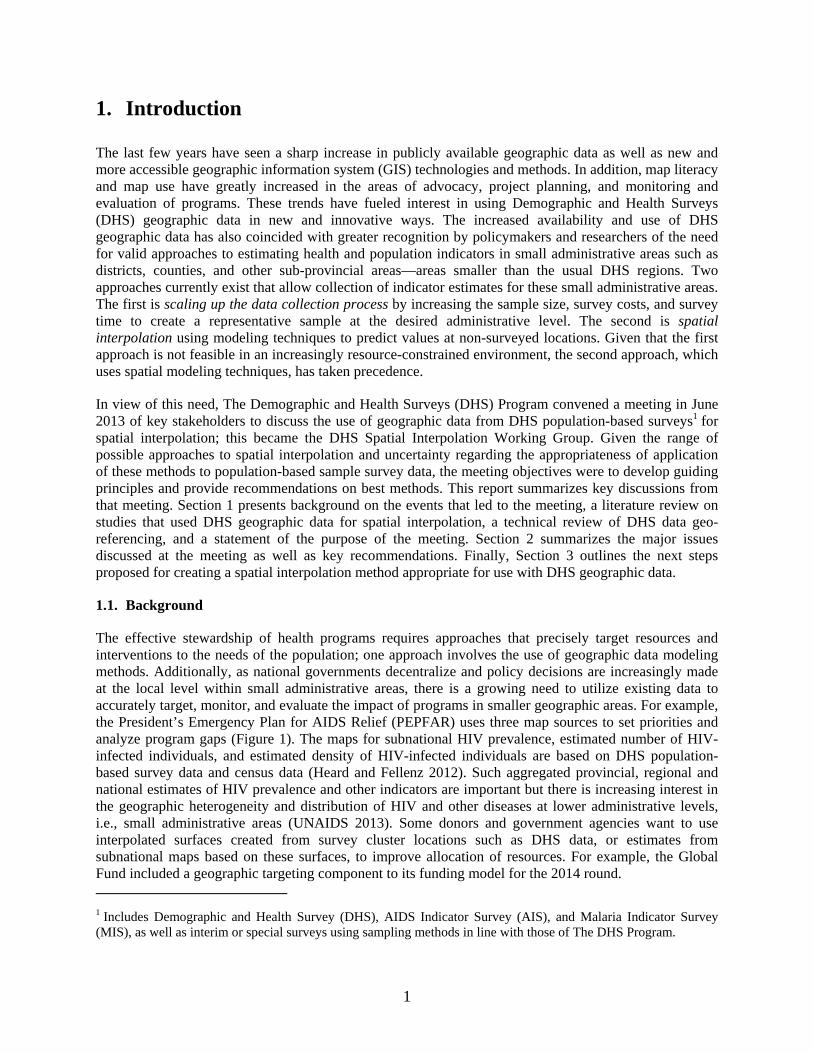
1. Introduction

The last few years have seen a sharp increase in publicly available geographic data as well as new and more accessible geographic information system (GIS) technologies and methods. In addition, map literacy and map use have greatly increased in the areas of advocacy, project planning, and monitoring and evaluation of programs. These trends have fueled interest in using Demographic and Health Surveys (DHS) geographic data in new and innovative ways. The increased availability and use of DHS geographic data has also coincided with greater recognition by policymakers and researchers of the need for valid approaches to estimating health and population indicators in small administrative areas such as districts, counties, and other sub-provincial areas—areas smaller than the usual DHS regions. Two approaches currently exist that allow collection of indicator estimates for these small administrative areas. The first is scaling up the data collection process by increasing the sample size, survey costs, and survey time to create a representative sample at the desired administrative level. The second is spatial interpolation using modeling techniques to predict values at non-surveyed locations. Given that the first approach is not feasible in an increasingly resource-constrained environment, the second approach, which uses spatial modeling techniques, has taken precedence.

In view of this need, The Demographic and Health Surveys (DHS) Program convened a meeting in June 2013 of key stakeholders to discuss the use of geographic data from DHS population-based surveys1 for spatial interpolation; this became the DHS Spatial Interpolation Working Group. Given the range of possible approaches to spatial interpolation and uncertainty regarding the appropriateness of application of these methods to population-based sample survey data, the meeting objectives were to develop guiding principles and provide recommendations on best methods. This report summarizes key discussions from that meeting. Section 1 presents background on the events that led to the meeting, a literature review on studies that used DHS geographic data for spatial interpolation, a technical review of DHS data geo-referencing, and a statement of the purpose of the meeting. Section 2 summarizes the major issues discussed at the meeting as well as key recommendations. Finally, Section 3 outlines the next steps proposed for creating a spatial interpolation method appropriate for use with DHS geographic data.

1.1. Background

The effective stewardship of health programs requires approaches that precisely target resources and interventions to the needs of the population; one approach involves the use of geographic data modeling methods. Additionally, as national governments decentralize and policy decisions are increasingly made at the local level within small administrative areas, there is a growing need to utilize existing data to accurately target, monitor, and evaluate the impact of programs in smaller geographic areas. For example, the President’s Emergency Plan for AIDS Relief (PEPFAR) uses three map sources to set priorities and analyze program gaps (Figure 1). The maps for subnational HIV prevalence, estimated number of HIV-infected individuals, and estimated density of HIV-infected individuals are based on DHS population-based survey data and census data (Heard and Fellenz 2012). Such aggregated provincial, regional and national estimates of HIV prevalence and other indicators are important but there is increasing interest in the geographic heterogeneity and distribution of HIV and other diseases at lower administrative levels, i.e., small administrative areas (UNAIDS 2013). Some donors and government agencies want to use interpolated surfaces created from survey cluster locations such as DHS data, or estimates from subnational maps based on these surfaces, to improve allocation of resources. For example, the Global Fund included a geographic targeting component to its funding model for the 2014 round. 1 Includes Demographic and Health Survey (DHS), AIDS Indicator Survey (AIS), and Malaria Indicator Survey (MIS), as well as interim or special surveys using sampling methods in line with those of The DHS Program.

2

Figure 1. PEPFAR example (Heard and Fellenz 2012) – Ethiopia: three ways of looking at HIV distribution

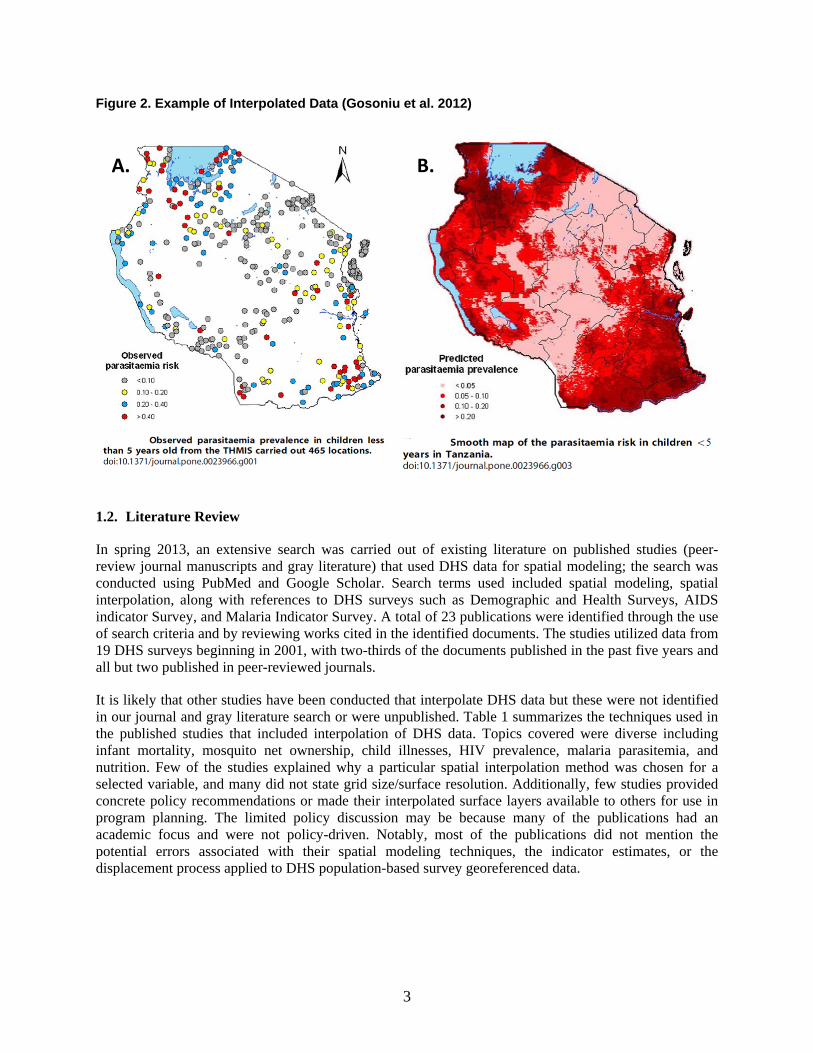
Spatial interpolation is one way to improve allocation of resources in program planning. It is a process in which a map surface is created by “estimating the values at unsampled points, based on known values of surrounding sampled points” (ESRI 2013). These interpolated outputs are in a raster or gridded surface format that represents values of a continuous surface. Some interpolation methods include external data in their models. These data, called “covariates,” may include population density, environmental factors such as rainfall or temperature, or access to roads. Some interpolation methods include error estimates that allow users of the new map surface to make their own decisions about the reliability of estimates. This structural flexibility can be important when estimates are used for downstream decision-making on the number of people in need of a specific service. Figure 2 shows an example of spatial interpolation using a Bayesian geostatistical model with data from the 2007-08 Tanzania HIV and Malaria survey (THMIS) sample points. Map A shows the observed cluster-level P. falciparum parasitemia prevalence values for children under five years; Map B shows the interpolated surface with predicted parasitemia prevalence for children under five years for the whole country (Gosoniu et al. 2012).

3

Figure 2. Example of Interpolated Data (Gosoniu et al. 2012)

1.2. Literature Review

In spring 2013, an extensive search was carried out of existing literature on published studies (peer-review journal manuscripts and gray literature) that used DHS data for spatial modeling; the search was conducted using PubMed and Google Scholar. Search terms used included spatial modeling, spatial interpolation, along with references to DHS surveys such as Demographic and Health Surveys, AIDS indicator Survey, and Malaria Indicator Survey. A total of 23 publications were identified through the use of search criteria and by reviewing works cited in the identified documents. The studies utilized data from 19 DHS surveys beginning in 2001, with two-thirds of the documents published in the past five years and all but two published in peer-reviewed journals.

It is likely that other studies have been conducted that interpolate DHS data but these were not identified in our journal and gray literature search or were unpublished. Table 1 summarizes the techniques used in the published studies that included interpolation of DHS data. Topics covered were diverse including infant mortality, mosquito net ownership, child illnesses, HIV prevalence, malaria parasitemia, and nutrition. Few of the studies explained why a particular spatial interpolation method was chosen for a selected variable, and many did not state grid size/surface resolution. Additionally, few studies provided concrete policy recommendations or made their interpolated surface layers available to others for use in program planning. The limited policy discussion may be because many of the publications had an academic focus and were not policy-driven. Notably, most of the publications did not mention the potential errors associated with their spatial modeling techniques, the indicator estimates, or the displacement process applied to DHS population-based survey georeferenced data.

A. B.

4

Table 1. Spatial modelling techniques applied in studies using DHS GPS data for spatial modelling and interpolation, publications 2001-2012

Technique Publication

Geo-additive regression (Kandala et al. 2006; Kazembe and Mpeketula 2010)

Geographically weighted regression model (Feldacker et al. 2010)

Kernel estimator (Larmarange 2011)

Spatial empirical Bayes estimation (Uthman 2008)

Inverse distance weighting (Gewa et al. 2013; Messina et al. 2010; Messina et al. 2011; Montana et al. 2007)

Nearest neighbor interpolation (Pande et al. 2008)

Conditional autoregressive model (Kazembe et al. 2007; Kazembe and Namangale 2007)

Geo-additive Probit and Latent Variable Model (Khatab and Fahrmeir 2009)

Bayesian generalized linear geostatistical model (Noor et al. 2010)

Bayesian Kriging (Gemperli et al. 2004; Gosoniu et al. 2010; Gosoniu et al. 2012)

Geo-additive semiparametric Bayesian model (Kandala et al. 2007; Kandala et al. 2001)

Geo-statistical Bernoulli & Gaussian models (Magalhães and Clements 2011)

Proportional hazards model with spatially correlated random effects

(Chin et al. 2011)

Zero-inflated Binomial model (Giardina et al. 2012)

1.3. Demographic and Health Surveys

The Demographic and Health Surveys (DHS) Program has earned a worldwide reputation for collecting and disseminating accurate, nationally representative data on fertility, family planning, maternal and child health, gender, HIV/AIDS, malaria, and nutrition. Data from the DHS household surveys are widely used to advance global understanding of health and population trends in developing countries and for planning and monitoring development programs. Since the beginning of the project in 1984, it has provided technical assistance to more than 300 surveys in over 90 countries and it is committed to making these data openly available. The survey has three main sections (1) Household questionnaire with household roster, (2) Individual questionnaire (typically all women 15-49 and a sub-sample of men 15-49), and (3) Biomarkers (anthropometric data (typically children < 5 years and women 15-49 years), anemia, HIV testing, and malaria parasite testing). The components of each section depend on the type of survey being implemented: Demographic and Health Survey (DHS), AIDS Indicator Survey (AIS), or Malaria Indicator Survey (MIS). Because the data structure is similar across these surveys we will refer to all three generically as DHS household surveys in this document.

The DHS household surveys use a two-stage cluster sampling design within each sample domain. Samples are designed to give indicator estimates that are nationally representative, as well as

5

representative at DHS subnational regions and urban/rural residence. DHS “regions” are subnational units defined for purposes of the survey that usually correspond to existing administrative units or groupings of these units. Increasingly, DHS household surveys are representative at lower levels of administrative units but currently these remain either administrative level 1 or level 2. The urban-rural “residence” of clusters is usually part of the sampling domain. Clusters are the primary sampling unit (PSU) for the survey and are preexisting, geographic groupings within the population. In the majority of DHS household surveys census enumeration areas (EAs) are defined by the country’s census bureau, along with the urban-rural status of clusters. An EA can be a city block or apartment building in urban areas, while in rural areas it is typically a village or group of villages. The population and size of sampled clusters vary within and between countries; typically, clusters contain 100 to 300 households, of which 20 to 30 households are randomly selected for survey participation.

The DHS Program started georeferencing coordinate data of cluster locations in the late 1980s, but only routinely so in the early 2000s. These georeferenced cluster-level datasets became available in the public domain in 2003. The estimated center of each cluster is recorded as a latitude-longitude coordinate from a Global Positioning System (GPS) receiver or directly from census EA boundary files or derived from public online maps or gazetteers. The georeferenced datasets can be linked to individual records in DHS household surveys through unique survey identifiers. For confidentiality purposes, the individual, household, and cluster identifiers are removed from the datasets of all household surveys prior to their public release. These standard respondent confidentiality measures are carried out on all three DHS household surveys. In addition, as part of this confidentiality process the geographic coordinates of the cluster are randomly displaced (Burgert et al. 2013). The displacement is as follows:

• Urban clusters are displaced a distance up to two kilometers.

• Rural clusters are displaced a distance up to five kilometers, with a further randomly selected 1% of the rural clusters displaced a distance up to ten kilometers.

Details on the DHS georeferenced data displacement process and the spatial variability of the resulting data can be found in Burgert et al. (2013). This displacement affects the use of the data in geospatial analysis in several ways, including: misclassification bias in measurement, errors in raster-based data extraction, and movement of points across geopolitical boundaries and natural borders. Details on error measurement and some possible approaches to correcting this problem are presented in DHS Spatial Analysis Report 8 (Perez-Heydrich et al. 2013).

1.4. DHS Spatial Interpolation Working Group Meeting

Within the context of greater availability of technology, the desire of decision-makers to use data at the level of small administrative units, the increased use of spatial modeling and interpolation techniques using DHS data in published literature, and the particularities of the DHS household survey georeferenced data, warrants careful consideration of the opportunities and limitations in the realm of interpolated map surfaces using DHS geographic location datasets.

In June 2013, The DHS Program brought together a working group of experts in spatial modeling methods for the “MEASURE DHS GIS Consultative Meeting.” The key aim of this meeting was to review approaches for creating interpolated (gridded) map surfaces using DHS variables.

6

The objectives of the meeting were to:

• Develop guiding principles for how best to use DHS georeferenced point data in creating interpolated map surfaces; and

• Provide recommendations on which method(s) to use to create interpolated map surfaces using DHS data.

Participants from universities in the United States and the United Kingdom, as well as the University of Namibia attended. Other participants included individuals from the U.S. Agency for International Development (USAID), the World Bank, other USAID cooperating agencies and contractors, and the U.S. Department of State. The participants and their affiliations are listed in Appendix A.

The meeting took place in Washington, D.C. from June 10 to June 12, 2013. Appendix B shows the first day agenda. The meeting began with DHS Program staff presenting on aspects of the DHS survey and georeferenced point data, including sampling methodology, displacement, and key survey terms. Then, other participants presented on the methods they have used to interpolate DHS or similar data. Finally, with the presentations as background, there were guided discussions that centered on the following key questions:

1. How does the 2-stage survey sample design influence spatial interpolation?

2. How should the hierarchical structure of household survey data be accounted for in spatial interpolation?

3. What determines optimum grid resolutions: georeferenced data displacement, survey sample, external covariates, indicator type, and/or level chosen for spatial interpolation?

4. Are some indicators easier/harder to interpolate (rare events, household level, etc.)?

5. How is the reference period of the data considered in spatial interpolation (past 2 weeks, past year, etc.)?

The discussions were lively and diverse and resulted in a long list of questions and issues to be considered. The questions were consolidated into a shorter list of main threads that were examined in depth in subsequent small and large group discussions over the next two days.

Throughout the meeting, there were vigorous and thorough discussions, highlighting different points of view within the working group. While participants reached consensus on some issues, the conclusions presented here do not necessarily encompass all the possible approaches for using DHS household survey data to create interpolated map surfaces.

7

2. Summary of Major Issues for Consideration

Two key themes emerged from the DHS Spatial Interpolation Working Group discussions, these centered on issues of data and methods. Data considerations included the selection of appropriate indicators for spatial interpolation while methods considerations focused on specific spatial interpolation techniques.

2.1. Data Considerations

Several data-related factors need consideration when using DHS data for spatial interpolation. Together, these factors should guide the use of DHS data for use in spatial interpolations and provide guidelines for judging the appropriateness of an indicator for this type of methodological approach. An indicator is defined in DHS as a statistic that measures a specific aspect of a population, program, or program objectives, activities, and outcomes. This section summarizes the key factors for consideration; it is not meant to be exhaustive.

2.1.1. Proposed guidelines for indicator selection

During the meeting, participants agreed on a list of general guidelines for selecting indicators for spatial interpolation (see Box 1.) Table 2 summarizes some of the most commonly used DHS indicators by topic area, indicator level (i.e., level of data collection), and whether the indicator was judged appropriate for interpolated surface mapping, according to meeting participants.

Box 1. Proposed guidelines for selection of indicators for spatial interpolation

The following indicator characteristics are proposed for selecting indicators suitable for spatial interpolation:

• Indicator measures well in DHS surveys—i.e., is a robust measurement not subject to significant recall error.

• Indicator does not measure a rare event (e.g., maternal mortality).

• Indicator is spatially distributed—i.e., varies across geographical space.

• Indicator has a specific reference period—not an indefinite reference period or reference period that is spatially linked to the outcome (e.g., ever tested for HIV, fever in the past two weeks).

• Indicator is not temporally or micro-seasonally restricted and, therefore, is not likely to change substantially over the course of data collection, which can last many months (e.g., school attendance, use of mosquito nets).

• Indicator relates to the current location of the respondent (e.g., not maternal mortality by the sisterhood method).

8

Table 2. Appropriateness of DHS indicators for spatial interpolation

Indicator Topic Area Indicator Level Appropriate for spatial Interpolation

Improved water source access Household characteristics

Household Yes

Improved sanitation facilities Household characteristics

Household Yes

Wealth index Household characteristics

Household Yes

Floor/roof/wall materials Household characteristics

Household Yes

Households with electricity Household characteristics

Household Maybe – DHS may not be best source of data

Secondary or higher education Education Individual woman Yes

Literacy Education Individual woman Yes

Total fertility rate Fertility Individual woman Maybe

Prevalence of modern contraceptive methods

Family planning Individual woman Yes

Unmet need for family planning Family planning Individual woman Yes – possible denominator issues

Age at 1st marriage Demography Individual woman Yes – among women 25-29

Age at 1st sex Demography Individual woman Yes – among women 25-29

Antenatal care (ANC) use Maternal health Individual woman Yes

Birth in health facility Maternal health Individual woman Yes

Infant mortality rate Demography (mortality)

Child Maybe

Under-five mortality rate Demography (mortality)

Child Maybe

Full immunization Child health Child Yes

Use of ORS for treatment of diarrhea

Child health Child No – short and non-static recall period (past 2 weeks)

Children <5 slept under ITN Malaria Child Yes – Malaria Indicator Survey or other survey done in proper season

Exclusive breastfeeding duration Nutrition Child Yes – among currently breastfeeding women (check question/definition)

Stunting among children <5 Nutrition Child Yes

Wasting among children <5 Nutrition Child No – short-term measure, hard to predict

Overweight women 15-49 Nutrition Individual woman Yes

Anemia Nutrition Individual woman/child

Yes

HIV prevalence HIV Individual Yes

HIV testing HIV Individual Yes – past year only

9

2.1.2. Robustness, rare events, and spatial distribution

In spatial interpolation with DHS data a cluster-level value (percentage, rate, or count) has to be calculated for each indicator and this value is then used for spatial modeling. The ability of the survey to measure an indicator well, the degree to which an indicator is common or rare, and the indicator’s spatial distribution, all play a role in creating reliable predictions about the underlying population.

The indicators selected for spatial interpolation must be robustly measured in the survey; that is, they should have low bias and be precisely and accurately measured at the cluster location. The possible biases associated with an indicator are recall bias and location bias. DHS survey questions have been tested over time and are designed to minimize recall bias. Location bias is discussed in the next section (Section 2.1.3). Spatial interpolation of clusters requires the calculation of a cluster-level point estimate (with associated standard error if possible). The survey sample is drawn so that the DHS survey domains are calculated with precision and accuracy; however, this does not mean that cluster-level data where there is a small number of individuals/households interviewed will have the same precision and accuracy as the sub-national domains. The standard errors of the point estimate can help data users understand the robustness of the estimate in any particular cluster or between clusters.

Rare events may differ between countries. An indicator can be rare in one country and common in another (e.g., female genital cutting, malaria prevalence). The rare event may occur in all clusters but with very few cases; thus, when only 30 households are sampled per cluster the sampling frame may not produce enough cases to randomly encounter the rare event. An interpolation surface map of this type of rare event may not adequately illustrate the true distribution of the event. In addition, indicators that are concentrated in space—that is rare or non-existent in some areas and more common in others—such as those occurring in urban areas only or in a specific region, may be considered rare for the country as a whole or too widely distributed, and thus be misleading when mapped. Additionally, both types of rare events can occur simultaneously in a country. Because cluster value can be based on a relatively small number of cases, the rarer the outcome the harder it is to have a precise estimate of the indicator at the cluster level. With interpolation, there is some difficulty showing high and low values within a population and “hot spots” end up being masked by the larger population distribution (Larmarange 2011).

Another case is when there is no spatial element or spatial distribution to the indicator; that is, there is no variability across a country or no difference between clusters that are in close proximity versus clusters that are far apart (as illustrated in a variogram, for example). Such a homogenous indicator can be interpolated but likely would not produce a useful map. Conversely, cluster value may have a variation of 100% (i.e., 95% confidence interval of 0-100%) at a specific cluster location or have a value of zero. Both cases may cause problems downstream in the spatial interpolation process. Though it may be possible to produce an interpolated map surface in these cases, the actual output will be of little value and can even be misleading if error estimates are not properly taken into account.

2.1.3. Reference period, temporality, and locality

The indicator reference period and its dependence on temporal and locational factors should be considered when assessing the indicator’s suitability for spatial interpolation. Most DHS indicators have a reference or recall period associated with them. This can vary from the present (i.e., time of the interview) to a two-week period preceding the survey, to the past year, to the past several years, to the course of a lifetime. Indicators with short recall periods, specifically those related to the “past two weeks”—a period mainly used in the child’s health section of the questionnaire—have the advantage of being very recent and specific; however, the “past two weeks” may not be equivalent for everyone in the same cluster, much less everyone in the survey. Frequently, data collection for a DHS survey can take anywhere from three to six months (or longer) to complete and any given cluster may take four to seven days to survey.

10

Clusters that are proximal to one another are not always surveyed at the same time and interviewing can be separated by several months.

The reference period and survey timing are particularly relevant for indicators that are temporally bounded or are specifically related to the time when the survey was conducted (e.g., rainy season, school year). These indicators include those related to the use of mosquito nets, parasitemia testing, diarrhea, dietary diversity, school attendance, and water source, among others. For the Malaria Indicator Survey (MIS), which includes parasite testing, survey planners try to reduce the temporal problem by scheduling data collection during the height of the malaria transmission season. However, seasonality varies within a country and from year to year and is sometimes difficult to take into account in survey planning and implementation. While it is not always be possible to correct for temporal issues, they need to be acknowledged and considered carefully when choosing an indicator for spatial interpolation. A multi-country analysis that compared the fieldwork periods of 169 DHS surveys with the rainy season in each country (and seasonal variation in rainfall), showed that the surveys were slightly more likely to be conducted in the dry season (Wright et al. 2012).

Locational bias involves attributing an event to have occurred in one place when in reality it occurred in a different place. This type of bias can occur when an event takes place in a different location from that of the respondent being interviewed; it can be minimized if the reference period is given proper consideration. DHS questionnaires prior to 2009 asked basic questions on migration that could be used to take into account some of these reference period issues. The questions were dropped from most surveys implemented from November 2009 onward. However, it is likely that these or similar migration questions will be introduced into the DHS core questionnaire during Phase 7 of The DHS Program. Shorter reference periods such as one year versus a lifetime are also likely to reduce locational bias.

The purpose of the interpolated map surface may be relevant when considering locational bias. For example, if an interpolated surface of women age 15-49 that were tested for HIV in the past 12 months was created, this surface may or may not accurately measure the impact of an HIV testing campaign in a specific area because some respondents may have been tested for HIV in a different location from the one where they were interviewed. However, if the surface was intended to be used to target future campaigns in areas with low levels of HIV testing, it might be a good targeting tool.

2.1.4. Other data considerations

Four other data considerations should be examined as they relate to specific spatial interpolation methods. These are not specific to indicator selection but rather to the structure and design of the survey.

• Spatial area: The cluster location data used in spatial interpolation are an estimated center of the survey cluster, a point location that actually represents an area of unknown size but with fairly large variability across a country, especially between urban and rural locations. In addition, these point locations are displaced from 0-2 km in urban locations and 0-5 km in rural locations, with 1% of rural locations displaced up to 10 km (Burgert et al. 2013). In many spatial interpolation methods the data are assumed to be discrete points instead of polygons areas. Although this assumption makes spatial interpolation easier, it also has implications for the spatial error of specific clusters that may be of different sizes.

• Survey weights: Interpolated modeling methods using DHS data need to account for the survey sampling weights. To date, most groups/researchers using DHS data have either ignored sampling weights in their spatial interpolations or failed to mention their use in the method descriptions (Magalhães and Clements 2011; Messina et al. 2011). While including sampling weights may not substantially change the interpolated surface outcome, it is good practice to include the survey

11

weights when using DHS data in analysis. Weighting the data is particularly important if the ultimate objective is to aggregate the surface to polygon units and use the estimated values for comparison across new “areas” instead of just creating interpolated map surfaces—for example, calculating a rate for a second-level administrative unit (district) from a survey that was representative at the first-level administrative unit.

• Multilevel survey design: The hierarchical structure of the DHS datasets is such that several individuals from a household can be included in the same indicator denominator. This intra-household correlation may be important to consider along with the intra-cluster correlation when creating interpolated map surfaces. For example, children in one specific household may be chronically malnourished while, on average, children in other households are not. However, this single household in the cluster may greatly influence the cluster-level estimate of chronic malnutrition.

• Indicator definition and denominator: It should be noted that definitions for some indicators, such as the anthropometry standards for children, have changed during the 30-plus years The DHS Program has been collecting survey data. Also, some countries have non-standard samples (ever-married women) that exclude unmarried women from fertility and family planning questions. While such differences do not prevent the mapping of data, they do limit comparability over time within or between countries.

2.2. Method Considerations

This section summarizes the broad guidelines agreed upon at the working group meeting regarding selection of spatial methods for creating an interpolated map surface with DHS data. The most important criteria for researchers using spatial interpolation methods with DHS data are 1) an accurate and statistically rigorous map, and 2) inclusion of a corresponding map surface with estimates of the uncertainty or potential error associated with the spatial interpolation.

2.2.1. Proposed guidelines for method selection

Box 2 lists the essential guidelines for choosing spatial interpolation methods for DHS data. In general, these guidelines exclude simpler interpolation algorithms often applied to univariate data such as inverse distance weighting and nearest neighbor interpolation because they do not include any information on uncertainty in the interpolated map surface created. It should be noted that this type of univariate spatial interpolation is in common use in the literature to date (Table 1). Inclusion of uncertainty estimates is important for analyzing the precision of the surface if the surface is aggregated to an administration unit for program target or used to estimate the number of people in need of a service.

12

Box 2. Proposed guidelines for method selection for DHS spatial interpolation

Other desirable but not essential guidelines for the DHS spatial interpolation method are that it should:

• Be fast (computationally efficient in memory and processing).

• Account for non-stationary variance (covariance/correlation varies as a function of the spatial location, e.g., urban and rural).

• Integrate space-time: ability to incorporate data from multiple surveys through time.

• Be able to aggregate uncertainty (the propagation of uncertainty when aggregated, to different administrative units or raster square size, i.e., conditional simulation).

• Account for support (the uncertainty in the size of the area represented by a cluster).

• Include formal covariate selection (have optimal covariate selection procedures).

• Account for poor adherence to commonly used sampling error models where necessary (e.g., consider zero inflation when excess zeros reduce the appropriateness of standard Poisson or binomial sampling models).

Beyond these essential and desirable guidelines, there are a number of other factors that should be considered and, if possible, integrated in some way into the selected method. These include edge effects, grid size, preferential sampling, non-Gaussian error, covariate quality, and survey nonresponse. Also, a range of considerations may need to be included to account for urban-rural issues. These include differential displacement, population density, and difference in spatial variability of outcome.

The method selected should have the following characteristics:

• Account for sampling variation: differences in the sample sizes of clusters.

• Include parameter uncertainty: errors in parameter estimation taken into account.

• Create uncertainty surface maps: produce standard errors/confidence intervals.

• Account for measurement error due to GPS displacement: error in geo-positions explicitly included in model.

• Incorporate explanatory covariates, where appropriate, such as temperature, land cover, and others.

• Account for spatial autocorrelation: spatially autocorrelated data (or residuals from a covariate model) violates the assumption of independence underlying most non-spatial methods.

• Include diagnostic statistics to evaluate model fits.

• Have high predictive capacity: good at predicting at unobserved locations/times.

• Use general linear model (GLM) because it can handle count, binary, binomial and continuous data.

• Be intuitive—the model should be easy to interpret for non-experts.

Tab

le 3

. Ess

enti

al a

nd

des

irab

le g

uid

elin

es f

or

spat

ial i

nte

rpo

lati

on

su

mm

ariz

ed b

y m

eth

od

Met

ho

d

Un

ivar

iate

Ap

pro

ach

(e

.g.,

IDW

) N

on

-sp

atia

l R

egre

ssio

n

Sm

all

Are

a E

stim

atio

n

Kri

gin

g

Au

tore

gre

ssi

ve

Met

ho

ds

Mo

del

-bas

ed

Geo

stat

isti

cs

Ess

enti

al

Sam

plin

g v

aria

tio

n

X

(if

MC

MC

* or

ML*

)X

X

(if M

CM

C o

r M

L)

X

(if M

CM

C o

r M

L)

Par

am

ete

r u

nce

rtai

nty

(bia

sed)

(p

ossi

ble)

X

(if M

CM

C o

r M

L)

X

(if M

CM

C o

r M

L)

Un

cert

ain

ty m

aps

(b

iase

d)

X

(pos

sibl

e)

X

(if M

CM

C o

r M

L)

X

(if M

CM

C o

r M

L)

Mea

sure

men

t er

ror

(dis

pla

cem

ent)

X

X

X

Inco

rpo

rate

co

vari

ate

s

X

X

X

X

X

Sp

atia

l au

toco

rrel

atio

n

X

X

X

X

Dia

gn

ost

ic s

tats

X

X

X

(if

MC

MC

or

ML)

X

(if

MC

MC

or

ML)

Hig

h p

red

icti

ve c

apac

ity

X

X

X

X

Gen

eral

ized

Lin

ear

Mo

del

X

X

X

X

Intu

itiv

e

X

X

X

Des

irab

le

Fas

t X

X

X

X

X

X

(if

in I

NLA

*)

No

n-s

tati

on

ary

vari

ance

X

(if in

INLA

)

Sp

ace-

tim

e in

teg

rati

on

X

X

X

Ag

gre

gat

able

un

cert

ain

ty

X

(if

con

ditio

nal

sim

ulat

ion)

X

X

Acc

ou

nti

ng

fo

r su

pp

ort

X

Fo

rmal

co

vari

ate

sele

ctio

n

X

X

X

X

Zer

o i

nfl

atio

n

X

X

X

*MC

MC

=M

arko

v C

hain

Mon

te C

arlo

, ML=

Max

imum

Lik

elih

ood

Est

imat

ion

, IN

LA=

Inte

grat

ed N

este

d La

plac

e A

ppro

xim

atio

ns

13

14

2.2.2. Selecting the best among the spatial interpolation methods

Many methods have been developed for creating interpolated map surfaces and several meet the guidelines laid out by the working group in Box 2. These methods and their ability to fulfill the essential and desirable guidelines are summarized in Table 3. The list is a compilation of methods employed by researchers using DHS data for spatial interpolation (Table 1). The two spatial interpolation methods the working group participants agreed best matched the guidelines laid-out were model-based geostatistics and to a lesser extent small area estimation (SAE). Importantly, both methods can provide parameter uncertainty estimates but these are not commonly produced for SAE. Autoregressive methods meet the majority of criteria but they require polygons as inputs which would necessitate converting DHS point data into polygons, information that is not available. Both autoregressive methods and SAE models are not continuous in space. They yield results that are aggregated in the form of polygons across space while model-based geostatistics produce raster gridded surfaces. Simple Kriging methods fit many guidelines outlined but do not provide parameter uncertainty estimates.

Selecting a specific method for spatial interpolation depends on a number of factors including 1) the type of question asked and indicator being used, 2) the covariates available for inclusion in the model, and 3) the structure of the input and output data. Figure 3 shows a decision tree that can assist in guiding the decision process for selecting a method. Most data are likely to fit the middle branch of the decision tree—a type of “mixed” approach. The best method might then be a hybrid between the SAE and the geostatistical methods. To date, no one has tried this type of hybrid approach with DHS data, but participants at the working group meeting agreed that, theoretically, it is possible. One potential drawback to using a model-based geostatistics approach is that the method crosses into the “inference” arena, while typically The DHS Program has stayed more within the “prediction” arena. An inference predicts outcomes using other data, some of which can be endogenous. Endogeneity occurs when the predicted variable is correlated with or related in some way to one or more variables used to create the prediction.

Meeting participants made a distinction between “best maps” for a specific country and “standardized maps” for the whole world in their discussions of potential methods for use in spatial interpolation. If the goal is to create the best map for a country using all available data, then SAE might be the best method, but only if detailed census data are available in a country. However, if the goal is to create standardized maps with publicly available covariate datasets, then the model-based geostatistical approach is likely the best method. Best maps would allow for the use of all the data relevant to a specific country; however, this approach limits somewhat the ability to compare the best map from country X with the best map from country Y because different covariate data, map resolution, and methods may be used. In addition, most countries do not routinely share detailed census data.

2.2.3. Measuring change over time

DHS data are often used to understand trends, however interpolated map surfaces of DHS data may not allow for direct comparison over time. This is because the survey sample changes, as do the sampling errors for each survey. Even if the same numbers of clusters are surveyed, they are unlikely to be in the same locations or to represent the same number of people. Thus, there is a non-comparable amount of measurement error that exists between the map surfaces. Administrative units change over time, complicating assessments of trends at lower administrative levels. Covariates evolve over time, for example, population density changes especially as populations become more urban, climate changes as annual specific rainfall varies, and new roads are created. Additionally, as better methods for data interpolation are developed, comparing two maps that were created using different underlying methods and covariates may be misleading. This is an area that will require further investigation, if researchers seek to compare change over time using interpolated map surfaces created independently.

15

Figure 3. Decision tree for selecting spatial interpolation methods for DHS geographic data

2.2.4. Covariate considerations

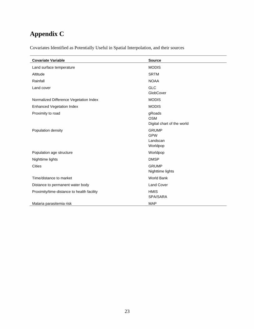
Covariates are important components of the interpolated methods identified as optimal for use with DHS data. Covariates are external data that are used to create a better prediction of the outcome of interest. These might include population density, night lights, environmental factors such as rainfall or temperatures, or access to roads. A non-exhaustive list of global-level covariates that might be included in a model applied to DHS data is shown in Appendix C. Covariates can have varying structure: raster (gridded surface of different resolution) or polygon area. Importantly, the covariates used must be available for the entire sampled/unsampled area that you are interpolating to, and must correspond to an appropriate time period that is referenced to the indicator being interpolated.

Most of the potential covariates that are relevant to indicators of interest are socio-economic or demographic in nature (e.g., education, employment status, number of births) as opposed to environmental or climatic factors (Figure 3). The best source for socio-economic covariates in many countries may be the DHS survey itself. Of course, great care should be taken in the event of using an interpolated surface map of a DHS indicator as covariate input in the spatial interpolation of another DHS indicator from the same survey. This is because there is a risk of circularity, or endogeneity, in inference, leading to confounding and, ultimately, erroneous maps. Considerations for including a covariate in an analysis include coverage, validity, uncertainty, access restrictions, spatial resolution, timing relative to

16

survey, source, endogeneity, and method for summarizing time-series data (snapshot, difference over time, or average).

Even if the covariates do not come from DHS data, care should be taken that they do not contain inputs that are similar to DHS inputs or are endogenous to the outcome of interest. For example, if you are using DHS data to produce an interpolated map surface of mortality, you may want to use a poverty surface map, but inputs to the poverty map may include data on mortality from a DHS or non-DHS source. Alternatively, one could rely on census data, vital statistics, demographic surveillance, or the results of other surveys; however, these data sources may not be available at a sufficiently fine-grained resolution, or with the same level of detail for all countries. Furthermore, often these datasets are not publicly available or do not have a spatial data component that allows for mapping at any scale.

Other aspects related to covariates may need to be considered prior to inclusion of a covariate in a spatial interpolation model. The underlying data resolution of the covariate raster may cause problems of misalignment. Urban and rural data may vary significantly or have different underlying mechanisms, which could require interaction terms or differential covariates. Finally, relying on others for covariate production, accuracy, and updating can cause delays or problems in producing maps in a timely manner.

17

3. Conclusion and Recommendations

Providing guidance on creating interpolated map surfaces using DHS data is an important task for The DHS Program in the coming years along with direction on the use and interpretation of these types of map surfaces. The June 2013 DHS Spatial Interpolation Working Group meeting was a step in a process that will lead to further collaboration between DHS and researchers worldwide and greater use of DHS data in the spatial realm.

The working group participants presented many and diverse perspectives on ways to create interpolated map surfaces. Each day the notes, summary tables, and figures produced by the small groups were collected and reviewed. The direction and scope of the smaller group discussions were based on earlier discussions or themes, and each small group had concrete tasks and outputs for each session. The conclusions presented here on spatial interpolation are those discussed at the meeting but they are probably not the only possible approaches. The working group participants agreed to two sets of guiding principles for how best to use DHS household survey georeferenced point data in creating interpolated map surfaces, one relating to the DHS indicator data selection and the other to method selection. These two sets of guidelines are outlined in Box 1 and 2, respectively. Of the many methods discussed, the meeting participants selected two as optimal for creating interpolated map surfaces with DHS data: model-based geostatistical methods and small area estimates. Beyond the need for accurate and statistically rigorous maps, the most important conclusion from the meeting was that regardless of method, it is essential that any interpolated map surface created using DHS data include corresponding uncertainty estimates.

Now that these spatial methods have been identified and considerations for interpolation have been described, comprehensive validation and sensitivity studies need to be carried out using the same datasets for the different methods.

Steps outlined by meeting participates for consideration in this exploratory process were as follows:

• Select 3 or 4 indicators to study; these should fit the indicator criteria set out above but also be from different indicator types, levels, and topic areas. These should include some of the most commonly used DHS indicators in the areas of nutrition, HIV, malaria, and fertility.

• Select 3 or 4 pilot countries to study; these should be geographically diverse but not surveys that include HIV testing.

• Select an appropriate list of covariates openly available on an international, regional, or country scale and run statistical tests for their association with the indicators for spatial interpolation without making any a priori assumptions about the causal pathways behind the association.

• Create basic methodological approaches that could work for all indicators and countries.

• Validate methods using proven techniques such as root-mean-square error (RMSE) and coverage probability of prediction interval (e.g., leave-one-out).

• Validate methods using undisplaced and displaced data points. (Undisplaced data are available for use in methodological studies of this type for surveys without HIV testing ONLY.)

• Conduct sensitivity analyses to compare the methods in urban and rural areas.

• Conduct sensitivity analyses of key covariates.

• Document the work and distribute results.

18

The working group discussed the pros and cons of The DHS Program producing its own interpolated map surfaces in the future. The group concluded that after completion of the exploratory process (described above), THE DHS Program should aim to routinely create interpolated map surfaces. If this activity is implemented by The DHS Program the recommendation of the group was that the maps should 1) use publicly available data, 2) be standardized across countries, 3) be easily reproducible, and 4) be created as comparable maps to facilitate policy and program decision-making. These spatial interpolation surface maps should be produced for a few indicators in each survey, along with comprehensive descriptions of methods and guidelines on data use and interpretation. Production of interpolated map surfaces by The DHS Program will not preclude other groups/researchers from doing the same, using either the DHS-validated method or other methods. The DHS Program encourages openness in code sharing and surface map sharing to broaden the use of these methods and the use of the map outputs for program planning and evaluation.

19

References

Burgert, C., J. Colston, T. Roy, and B. Zachary. 2013. Geographic Displacement Procedure and Georeferenced Data Release Policy for the Demographic and Health Surveys. DHS Spatial Analysis Reports No. 7. Calverton, Maryland, USA: ICF International.

Chin, B., L. Montana, and X. Basagana. 2011. "Spatial Modeling of Geographic Inequalities in Infant and Child Mortality across Nepal." Health and Place 17(4): 929-36.

ESRI. 2013. GIS Dictionary: Interpolation. ESRI 2013. Available online at http://support.esri.com/en /knowledgebase/GISDictionary/term/interpolation, accessed on September 17, 2013.

Feldacker, C., M. Emch, and S. Ennett. 2010. "The Who and Where of HIV in Rural Malawi: Exploring the Effects of Person and Place on Individual HIV Status." Health and Place 16(5): 996-1006.

Gemperli, A., P. Vounatsou, I. Kleinschmidt, M. Bagayoko, C. Lengeler, and T. Smith. 2004. "Spatial Patterns of Infant Mortality in Mali: The Effect of Malaria Endemicity." American Journal of Epidemiology 159(1): 64-72.

Gewa, C.A., T.F. Leslie, and L.R. Pawloski. 2013. "Geographic Distribution and Socio-Economic Determinants of Women's Nutritional Status in Mali Households." Public Health Nutrition 16(9): 1575-85.

Giardina, F., L. Gosoniu, L. Konate, M.B. Diouf, R. Perry, O. Gaye, O. Faye, and P. Vounatsou. 2012. "Estimating the Burden of Malaria in Senegal: Bayesian Zero-Inflated Binomial Geostatistical Modeling of the MIS 2008 Data." PLoS ONE 7(3): e32625.

Gosoniu, L., A.M. Veta, and P. Vounatsou. 2010. "Bayesian Geostatistical Modeling of Malaria Indicator Survey Data in Angola." PLoS ONE 5(3): e9322.

Gosoniu, L., A. Msengwa, C. Lengeler, and P. Vounatsou. 2012. "Spatially Explicit Burden Estimates of Malaria in Tanzania: Bayesian Geostatistical Modeling of the Malaria Indicator Survey Data." PLoS ONE 7(5): e23966.

Heard, N.J., and C.L. Fellenz. 2012. "Ethiopia: Three Ways of Looking at HIV Distribution." In Demographic and Health Survey Spatial Data Repository, edited by Demographic and Health Survey Spatial Data Repository. Washington D.C., USA: HumanitarianInformaiton Unit, U.S. Department of State.

Kandala, N.B., C. Ji, N. Stallard, S. Stranges, and F.P. Cappuccio. 2007. "Spatial Analysis of Risk Factors for Childhood Morbidity in Nigeria." American Journal of Tropical Medicine and Hygiene 77(4): 770-9.

Kandala, N.B., S. Lang, S. Klasen, and L. Fahrmeir. 2001. Semiparametric Analysis of the Socio-Demographic and Spatial Determinants of Undernutrition in Two African Countries. Collaborative Research Center Discussion Paper No. 245. Munich, German: Ludwig Maximilians University of Munich.

Kandala, N.B., M.A. Magadi, and N.J. Madise. 2006. "An Investigation of District Spatial Variations of Childhood Diarrhoea and Fever Morbidity in Malawi." Social Science and Medicine 62(5): 1138-52.

20

Kazembe, L.N., C.C. Appleton, and I. Kleinschmidt. 2007. "Geographical Disparities in Core Population Coverage Indicators for Roll Back Malaria in Malawi." International Journal for Equity in Health 6:5.

Kazembe, L.N., and P.M. Mpeketula. 2010. "Quantifying Spatial Disparities in Neonatal Mortality Using a Structured Additive Regression Model." PLoS ONE 5(6): e11180.

Kazembe, L.N., and J.J. Namangale. 2007. "A Bayesian Multinomial Model to Analyse Spatial Patterns of Childhood Co-Morbidity in Malawi." European Journal of Epidemiology 22(8): 545-56.

Khatab, K., and L. Fahrmeir. 2009. "Analysis of Childhood Morbidity with Geoadditive Probit and Latent Variable Model: A Case Study for Egypt." American Journal of Tropical Medicine and Hygiene 81(1): 116-28.

Larmarange, J., R. Vallo, S. Yaro, P. Msellati, and N. Méda, 2011. "Methods for Mapping Regional Trends of HIV Prevalence from Demographic and Health Surveys (DHS)." Cybergeo: European Journal of Geography: 558.

Magalhães, R.J.S., and A.C.A. Clements. 2011. "Mapping the Risk of Anaemia in Preschool-Age Children: The Contribution of Malnutrition, Malaria, and Helminth Infections in West Africa." PLoS Medicine 8(6): e1000438.

Messina, J.P., M. Emch, J. Muwonga, K. Mwandagalirwa, S.B. Edidi, N. Mama, A. Okenge, and S.R. Meshnick. 2010. "Spatial and Socio-Behavioral Patterns of HIV Prevalence in the Democratic Republic of Congo." Social Science and Medicine 71(8): 1428-35.

Messina, J.P., S.M. Taylor, S.R. Meshnick, A.M. Linke, A.K. Tshefu, B. Atua, K. Mwandagalirwa, and M. Emch. 2011. "Population, Behavioural and Environmental Drivers of Malaria Prevalence in the Democratic Republic of Congo." Malaria Journal 10: 161.

Montana, L., M. Neuman, and V. Mishra. 2007. Spatial Modeling of HIV Prevalence in Kenya. DHS Working Papers No. 27. Calverton, Maryland, USA: Macro International Inc.

Noor, A.M., V.A. Alegana, A.P. Patil, and R.W. Snow. 2010. "Predicting the Unmet Need for Biologically Targeted Coverage of Insecticide-Treated Nets in Kenya." American Journal of Tropical Medicine and Hygiene 83(4): 854-60.

Pande, S., M.A. Keyzer, A. Arouna, and B.G. Sonneveld. 2008. "Addressing Diarrhea Prevalence in the West African Middle Belt: Social and Geographic Dimensions in a Case Study for Benin." International Journal of Health Geographics 7: 17.

Perez-Heydrich, C., J.L. Warren, C.R. Burgert, and M.E. Emch. 2013. Guidelines on the Use of DHS GPS Data. Spatial Analysis Reports No. 8. Calverton, Maryland, USA: ICF International.

UNAIDS. 2013. Location, Location: Connection People Faster with Services. Geneva, Switzerland: Joint United Nations Programme on HIV/AIDS (UNAIDS).

Uthman, O.A. 2008. "Geographical Variations and Contextual Effects on Age of Initiation of Sexual Intercourse among Women in Nigeria: A Multilevel and Spatial Analysis." International Journal of Health Geographics 7: 27.

Wright, J.A., H. Yang, and K. Walker. 2012. "Do International Surveys and Censuses Exhibit ‘Dry Season’ bias?" Population, Space and Place 18(1): 116-26.

21

Appendix A

DHS Spatial Interpolation Working Group

Name Institution

Victor Alegana KEMRI-Welcome Trust Research Programme, Kenya

Fred Arnold The DHS Program, ICF International

Pete Atkinson University of Southampton, United Kingdom

Deborah Balk Baruch College, City University of New York

Noah Bartlett USAID, The DHS Program Management Team

Samir Bhatt University of Oxford, United Kingdom

Clara R. Burgert The DHS Program, ICF International

Marcia Castro Harvard School of Public Health

Josh Colston The DHS Program, ICF International

Mike Emch University of North Carolina at Chapel Hill

Pete Gething University of Oxford, United Kingdom

Nathan Heard U.S. Department of State, Humanitarian Information Unit

Andrew Inglis MEASURE Evaluation, John Snow, Inc.

Mark Janko Population Center, University of North Carolina

Lawrence Kazembe University of Namibia

Andrew Lawson Medical University of South Carolina

Mark Montgomery Population Council

Maria Muniz Center for International Earth Science Information Network (CIESIN), Columbia University

Soibhan Murray World Bank

Carolina Perez-Heydrich Population Center, University of North Carolina

Carla Pezzulo University of Southampton, United Kingdom

Tom Pullum The DHS Program, ICF International

Ruilin Ren The DHS Program, ICF International

Shadrock Roberts USAID GeoCenter

Thea Roy The DHS Program, Blue Raster

Shea Rutstein The DHS Program, ICF International

John Spencer MEASURE Evaluation, University of North Carolina at Chapel Hill

Andy Tatem University of Southampton, United Kingdom

Gary Watmough Earth Institute, Columbia University

Dan Weiss University of Oxford, United Kingdom

22

Appendix B

DHS Spatial Interpolation Working Group - Meeting Agenda: Day 1

Day 1: June 10

Session Presenter Start End

8:30 9:00 Arrival

9:00 9:30 Introductions & Agenda Review Clara Burgert

9:30 10:00 Meeting Objectives & Issue Overview Clara Burgert & Fred Arnold

10:00 10:15 DHS Displacement Thea Roy

10:15 10:30 Literature Review Josh Colston

10:30 10:45 Data Use Implications Nate Heard

10:45 11:00 Break

11:00 11:45 GPS Basic Methods Use Case Paper & Interpolated Methods Overview & DHS Relevance

Mike Emch, Carolina Perez-Heydrich, & Mark Janko

11:45 12:00 Data Use Implications Mark Montgomery

12:00 12:30 DHS Sampling Ruilin Ren

12:30 1:15 Lunch

1:15 1:30 Data Integration/Resolution Deborah Balk

1:30 1:45 Method Presentation: Child Health Lawrence Kazembe

1:45 2:00 Method Presentation: Malaria Victor Alegana

2:00 2:15 Method Presentation: Interpolation Pete Atkinson

2:15 2:40 Method Presentation: MAP Pete Gething & Samir Bhatt

2:40 3:05 Method Presentation: Poverty Andy Tatem, Carla Pezzulo, & Dan Weiss

3:05 3:15 Recap & Questions Clara Burgert

3:15 3:30 Break

3:30 5:00 Guided Discussion Clara Burgert

5:00 5:15 Group Creation & Tasking Clara Burgert

5:15 5:30 Logistics Josh Colston

23

Appendix C

Covariates Identified as Potentially Useful in Spatial Interpolation, and their sources

Covariate Variable Source

Land surface temperature MODIS

Altitude SRTM

Rainfall NOAA

Land cover GLC GlobCover

Normalized Difference Vegetation Index MODIS

Enhanced Vegetation Index MODIS

Proximity to road gRoads OSM Digital chart of the world

Population density GRUMP GPW Landscan Worldpop

Population age structure Worldpop

Nighttime lights DMSP

Cities GRUMP Nighttime lights

Time/distance to market World Bank

Distance to permanent water body Land Cover

Proximity/time-distance to health facility HMIS SPA/SARA

Malaria parasitemia risk MAP