DEVELPOMENT OF A COMPREHENSIVE EXCEL

SPREADSHEET FOR ESTIMATING THE OUTPUT OF SOME

GEOTECHNICAL LABORATORY EXPERIMENTS

A THESIS SUBMITTED

IN PARTIAL FULFILMENT OF THE REQUIREMENT

FOR THE AWARD OF THE DEGREE

OF

BACHELOR OF TECHNOLOGY

IN

CIVIL ENGINEERING

Submitted by under the guidance of

Jyotishman Mudiar (111CE0424) Dr. R N Behera

B.Tech. Dept. of Civil Engineering, Dept. of Civil Engineering.

NIT Rourkela NIT Rourkela

2 | P a g e

CERTIFICATE

National Institute Of Technology

Rourkela

This certificate is to state that “DEVELPOMENT OF A COMPREHENSIVE EXCEL

SPREADSHEET FOR ESTIMATING THE OUTPUT OF SOME GEOTECHNICAL

LABORATORY EXPERIMENTS” is an original and sincere work carried out by Jyotishman

Mudiar under my supervision in partial fulfilment of the degree of Bachelor of Technology under

the Dept. of civil engineering, NIT Rourkela, Odisha.

It is also certified that the work of this project has not been submitted elsewhere for the award

of any degree or diploma.

Place: Rourkela Dr Rabi Narayan Behera

Date: Department of Civil Engineering

3 | P a g e

ACKNOWLEDGEMENT

At the very outset, I would like to express my sincere gratitude to my supervisor Dr. Rabi

Narayan Behera for all his support and guidance throughout the course of my work in last one

year.

I would also like to take out a moment to thank Mr. A. K Nanda, Technical Assistant,

Geotechnical Engineering Laboratory, NIT Rourkela for his able guidance during my work.

Last but not the least, I am very much thankful to my friend Tanzim Hussain and Jeet

Mohapatra, students of NIT Rourkela for their technical support in Microsoft Excel and

Microsoft Power Point.

Jyotishman Mudiar

(111CE0424)

4 | P a g e

Abstract

Geotechnical laboratory experiments are vital in determining the geotechnical properties of

soil. These tests are generally performed for a number of times to obtain the best result and in most

of the times, to average them to minimize the deviation in output. Hence to execute the process

calculation is a tedious and hectic process, especially when the number of experiments is large or

the steps of calculations are lengthy. Besides, the availability of software and spreadsheets to

obtain accurate output is very rare in literature, and the few that are there are too in-comprehensive

and incomplete dealing just a few of the many laboratory experiments that the entire geotechnical

engineering is concerned.

The work in this project is an honest effort to minimize the effort involved in the different

Civil engineering laboratory experiments carried out at different institutes and construction sectors

by designing a Microsoft Excel Spreadsheet that determines the output of the different

geotechnical laboratory experiments along with the graph of related parameters wherever

necessary. The process, procedure, input parameters and the calculations have been followed as

per the Indian Standard Codes of Geotechnical Engineering. In cases, where the size of the

apparatus or the related constants vary from place to place, the input columns have been provided

where the different input can be incorporated in order to obtain the corresponding result.

The excel spread sheet has been designed to make it a generalized one so that the utility of

this spread sheet can be availed irrespective of variation in location and instruments. For all

practical reference during the work, the Geotechnical Engineering Laboratory of NIT Rourkela

has been used and the output has been tested on a number of inputs that were obtained in different

experiments done at NIT Rourkela. The result obtained has been found consistent. Also a few

inputs of the book, “Principles Of geotechnical Engineering” by B M Das and “Soil Mechanics

and foundations” by B C Punmia, Ashok Kr. Jain, Arun Kr. Jain have been tested and found

consistent.

Hence, this Microsoft Excel Spread sheet can be judiciously used in minimizing effort and

obtaining the most accurate outputs in various laboratory experiments in Geotechnical

Engineering.

5 | P a g e

CONTENTS

Certificate 2

ACKNOWLEDGEMENT 3

ABSTRACT 4

CONTENTS 5

LIST OF FIGURES 6

LIST OF TABLES 7

CHAPTER 1

INTRODUCTION 8

CHAPTER 2

SCOPE AND OBJECTIVE 9

CHAPTER 3

GEOTECHNICAL LABORATORY TESTS AND THEIR EXCEL SPREADSHEET

DETERMINATION (METHODOLOGY) 10-41

CHAPTER 4

CONCLUSION 42

CHAPTER 5

REFERENCE 43

6 | P a g e

LIST OF FIGURES

1. Fig 3.1 (a) STANDARD LIQUID LIMIT APARATUS PAGE-9

2. Fig 3.2 (a), (b) STANDARD SHRINKAGE LIMIT APARATUS PAGE-12

3. Fig 3.4 (a), (b) APARATUS FOR STANDARD PROCTOR TEST PAGE-16

4. Fig 3.5 (a) APARATUS FOR CORE CUTTER METHOD PAGE-18

5. Fig 3.6 (a) APARATUS FOR SAND REPLACEMENT METHOD PAGE-20

6. Fig 3.7 (a) APARATUS FOR HYDROMETER ANALYSIS PAGE-27

7. Fig 3.9 (a) APARATUS FOR VARIABALE HEAD TEST PAGE-32

7 | P a g e

LIST OF TABLES

1. TABLE 3.1 LIQUID LIMIT PAGE-11

2. TABLE 3.2 SHRINKAGE LIMIT PAGE-13

3. TABLE 3.3 SPECIFIC GRAVITY PAGE-15

4. TABLE 3.4 LIGHT COMPACTION PAGE-17

5. TABLE 3.5 CORE CUTTER PAGE-19

6. TABLE 3.6 SAND REPLACEMENT PAGE-21

7. TABLE 3.7 DIRECT SHEAR PAGE-23

8. TABLE 3.8 VANE SHEAR PAGE-25

9. TABLE 3.9(a) SIEVE ANALYSIS PAGE-26

10. TABLE 3.9(b) HYDROMETER ANALYSIS PAGE-28

11. TABLE 3.9(c ) GRAIN SIZE DISTRIBUTION PAGE-29

12. TABLE 3.10 CONSTANT HEAD PERMEABILITY PAGE31

13. TABLE 3.11 VARIABLE HEAD PERMEABILITY PAGE-32

14. TABLE 3.12 TRIAXIAL SHEAR TEST PAGE-36

15. TABLE 3.13 LOAD BEARING CAPACITY OF FOUNDATION PAGE-40

8 | P a g e

INTRODUCTION CHAPTER 1

In general soil is a later stage of rock cycle when withered successively. They are aggregates

of mineral particles, and together with air or water or both in the void spaces, form the three phase

system The different physical properties of soil depends on different factors like the type of

minerals that constitute them, the physical conditions they are subjected to, the extent of withering

the rock cycle has reached etc. Based on these factors, soil exhibits different geotechnical

properties. Grain-size distribution, specific gravity, water content, cohesion, load bearing capacity

are a few common properties that we come across in all aspects of geotechnical engineering.

Geotechnical Engineering is a branch of civil engineering that involves materials found close

to earth’s surface. It includes the application of soil mechanics in design of different structures like

foundations, retaining structures, earth structures, embankments etc.

In the ancient times, the geotechnical engineering was based on the artistic perspective and

the perceptions based on past experiences. The true geotechnical engineering came after

Skempton, 1985 which not only mitigated many common flaws that used to occur frequently in

design structures of the past, but also led to the invention of many wonderful engineering marvels.

This modern geotechnical engineering is based on detailed laboratory experiments for the

determination of different geotechnical properties of soil used in construction sites.

These geotechnical properties play vita roles and are of immense utility in all the

construction sectors like roads, embankments, bridges, buildings etc. They play a significant role

in determining the sustainability and stability of a structure, in determining the different types of

design to be used corresponding to different sites, in selecting construction sites, in estimating the

types of landfill liners or geo-synthetics to be used in low lying areas etc.

Hence, the laboratory experiments of the geotechnical properties are significant and vital to

every construction sector.

9 | P a g e

SCOPE AND OBJECTIVE CHAPTER 2

The objective of this project work is to design a comprehensive excel spread sheet that can

estimate the output of some geotechnical laboratory experiments with less effort and utmost

accuracy.

The scope of this work is that it can be used effortlessly and effectively in different

geotechnical engineering institutes and construction sectors to obtain the output in experiments for

which the spread sheet has been developed.

10 | P a g e

GEOTECHNICAL LABORATORY EXPERIMENTS CHAPTER 3

3.1

LIQUID LIMIT (LL) : (IS 2720-part 5, 1985.)

The moisture content at the point which transmission from plastic to liquid state takes place in a

soil system is the liquid limit.

Fig 3.1(a) Liquid Limit Apparatus (Das, B. M., 2010)

To perform the liquid limit test, one must place a soil paste in the cup. A groove is then cut at the

center of the soil pat with the standard grooving tool. The moisture content, in percent, required to

close a distance of 12.7 mm (0.5 in.) along the bottom of the groove after 25 blows is defined as

the liquid limit. The relationship between moisture content and log N is approximated as a straight

line. This line is referred to as the flow curve (Das, B. M., 2010). The moisture content

corresponding to N=25, determined from the flow curve, gives the liquid limit of the soil. The

slope of the flow line is defined as the flow index and may be written as

IF = (w1-w2)/Log(N2/N1)

Where IF= flow index

w represents water content, N represent number of blows.

11 | P a g e

EXCEL SPREAD SHEET DEVELOPMENT

Input parameters:

1. Weight of moist soil+ tin =B

2. Weight of dry soil+ tin=C

3. Weight of tin=D

4. Number of blows=H

Output parameters:

1. Weight of dry soil=C-D=E

2. Weight of water=B-D-E=F

3. Moisture Content=F*100/E=G

4. Flow Index=obtained from slope of curve:

5. Liquid Limit. = water content corresponding to 25 blows.

Algorithm to get as the cell output.

Step: 1: Moisture content G is obtained for 5 different inputs and is averaged.=y1.

Step: 2: Number of blows H is taken corresponding to the 5 inputs,averaged =x1

Step 3: slope is calculated by taking G as ordinates and H as abscissas, then averaged=m

Step 4: LL= y1+m*(25-x1)

Snapshot of designed spread sheet (table 3.1)

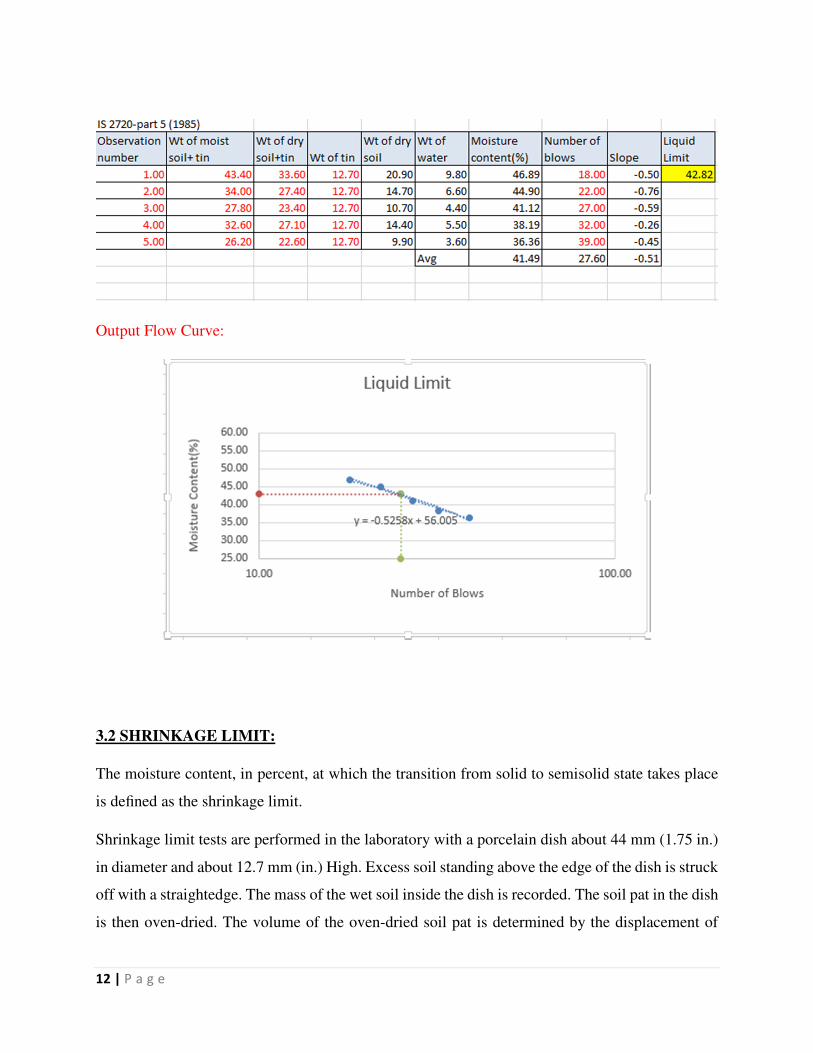
12 | P a g e

Output Flow Curve:

3.2 SHRINKAGE LIMIT:

The moisture content, in percent, at which the transition from solid to semisolid state takes place

is defined as the shrinkage limit.

Shrinkage limit tests are performed in the laboratory with a porcelain dish about 44 mm (1.75 in.)

in diameter and about 12.7 mm (in.) High. Excess soil standing above the edge of the dish is struck

off with a straightedge. The mass of the wet soil inside the dish is recorded. The soil pat in the dish

is then oven-dried. The volume of the oven-dried soil pat is determined by the displacement of

13 | P a g e

mercury. The wax-coated soil pat is then cooled. Its volume is determined by submerging it in

water (Das, B. M., 2010).

Fig. 3.2: A schematic diagram of apparatus of shrinkage limit test (Das, B. M., 2010)

Shrinkage limit can then be calculated by the formula given below

SL= ((M1-M2)/M2)*100- ((Vi-Vf)/M2)*Dw*100

Where M1= mass of wet soil pat in dish in beginning

M2= mass of dry soil pat

Vi=initial volume of wet soil pat

Vf= final volume of oven dried soil

Dw= desnity of water.

EXCEL SPREAD SHEET DEVELOPMENT

Input parameters

1. Weight of shrinkage dish + wet soil =A

2. Weight of dish+ dry soil =B

3. Weight of dish alone=C

4. Weight of mercury to fill dish=D

5. Weight of mercury displace by dry soil=F

14 | P a g e

Output parameters

1. Original volume of wet soil=E=D/13.6

2. Dry volume of soil=G=F/13.6

3. Initial moisture content (%)=H=100*(A-B)/(B-C)

4. Shrinkage Limit=SL= (H-100*(E-G)/(B-C))

*average of 4/5 experiments are taken to minimize deviation.

Snapshot of the excel spreadsheet determined for shrinkage limit( table 3.2)

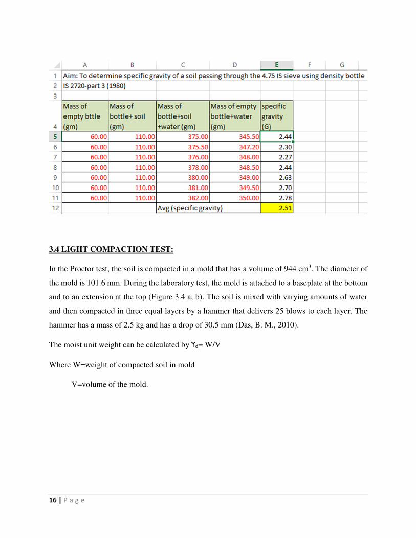
3.3 SPECIFIC GRAVITY (G):

Specific gravity is defined as the ratio of the unit weight of a given volume of dry soil in air to the

unit weight of equal volume of distilled water at 270C (Das, B. M., 2010).

In laboratory, the soil sample is taken in a bottle of known weight and the soil in weighed. Then

water is poured to half the mark and shacked well to blow out the air and then filled to the top and

weighed. Next soil-water mixture is thrown and water is poured into it and weighed.

Specific gravity G is obtained by: w1/ (w1-w3+w2)

15 | P a g e

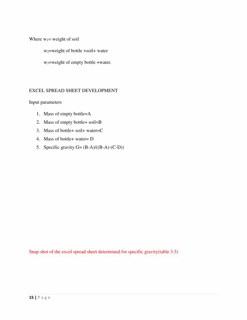
Where w1= weight of soil

w2=weight of bottle +soil+ water

w3=weight of empty bottle +water.

EXCEL SPREAD SHEET DEVELOPMENT

Input parameters

1. Mass of empty bottle=A

2. Mass of empty bottle+ soil=B

3. Mass of bottle+ soil+ water=C

4. Mass of bottle+ water= D

5. Specific gravity G= (B-A)/((B-A)-(C-D))

Snap shot of the excel spread sheet determined for specific gravity(table 3.3)

16 | P a g e

3.4 LIGHT COMPACTION TEST:

In the Proctor test, the soil is compacted in a mold that has a volume of 944 cm3. The diameter of

the mold is 101.6 mm. During the laboratory test, the mold is attached to a baseplate at the bottom

and to an extension at the top (Figure 3.4 a, b). The soil is mixed with varying amounts of water

and then compacted in three equal layers by a hammer that delivers 25 blows to each layer. The

hammer has a mass of 2.5 kg and has a drop of 30.5 mm (Das, B. M., 2010).

The moist unit weight can be calculated by ϒd= W/V

Where W=weight of compacted soil in mold

V=volume of the mold.

17 | P a g e

Figure 3.4 A schematic diagram of apparatus of a standard proctor test (adapted from “principles

of geotechnical Engineering” B M Das)

EXCEL SPREAD SHEET DEVELOPMENT

Input parameters

1. Weight of container= A

2. Weight of wet soil+ container=B

3. Weight of container+ dry soil= C

4. Weight of mold=F

5. Weight of mold +wet soil=G

Output parameters

1. Water content=D= (B-C)*100/(C-A)

2. Dry density ϒd = (G-F)*0.001/(1+(D*0.01))

18 | P a g e

Snapshot of the excel spread sheet designed for standard proctor test( table 3.4)

Curve obtained from the above spread sheet.

3.5 CORE CUTTER METHOD TO EVALUATE IN-SITU DRY DENSITY:

This test is done to determine the in-situ dry density of soil by core cutter method as per IS: 2720

(Part XXIX) – 1975

19 | P a g e

Fig 3.5 (a)

Procedure to determine the In-Situ Dry Density of Soil by Core Cutter Method

i) The internal volume (V) of the core cutter in cc should be calculated from its dimensions which

should be measured to the nearest 0.25mm.

ii) The core cutter should be weighed to the nearest gram (W1).

iii) The cutter containing the soil core should be weighed to the nearest gram (W2).

iv) The soil core should be removed from the cutter and a representative sample should be placed

in an air-tight container and its water content (w).

Formulas used

Bulk density of the soil g/cc ϒ = [W2 – W1]/ V g/cc

Dry density of the soil g/cc ϒd = 100Y/[100+w] g/cc

EXCEL SPREAD SHEET DEVELOPMENT

Input parameters:

1. Weight of core cutter=A

20 | P a g e

2. Weight of core cutter with soil=B

3. Weight of moisture=C

4. Volume of core cutter=E

Output parameters:

1. Weight of weight soil=D

2. Bulk Density= D/E

Snapshot of the excel spread sheet designed for core cutter method (3.5)

3.6 SAND REPLACEMENT METHOD TO EVALUATE IN-SITU DRY DENSITY:

This test is done to determine the in-situ dry density of soil by sand replacement method as per IS:

2720 (Part XXVIII) – 1974.

21 | P a g e

Fig 3.6 (a) Schematic view of Sand replacement apparatus

In laboratory test, a pit is excavated into the ground, through the hole in the plate, approximately

12 cm deep (same as the height of the calibrating can). The hole in the tray will guide the diameter

of the pit to be made in the ground. The excavated soil is collected into the tray and weighed (W).

Moisture content is then determined. The Sand penetrating cylinder with sand is weighed and

finally after letting the sand to run into the pit by opening the slit of SPC, the weight of the SPC

with the remaining sand (W4) is taken.

EXCEL SPREADSHEET DETERMINATION FOR SAND RELACEMENT METHOD

Input parameters

1. Weight of sand+ cone=A

2. Mean weight of sand in cone=B

3. Volume of calibrating container=C

4. Weight of sand+ cylinder after pouring=D

5. Weight of weight soil from hole=G

6. Weight of sand +cylinder after pouring into hole=H

Output parameters

1. Weight of sand filling container=A-B-D=E

2. Bulk density=E/C=F

3. Weight of sand into hole=A-B-H=I

4. Bulk density=G*F/I

22 | P a g e

Snap shot of the excel spread sheet determined for sand replacement method to evaluate in-situ

dry density.( Table 3.6)

3.7 DIRCT SHEAR TEST:

The direct shear test is one of the most commonly used techniques for determining the shear

strength parameters of soil.

The test is performed on three or four specimens from a relatively undisturbed soil sample .A

specimen is placed in a shear box which has two stacked rings to hold the sample; the contact

between the two rings is at approximately the mid-height of the sample. A confining stress is

applied vertically to the specimen, and the upper ring is pulled laterally until the sample fails, or

through a specified strain. The load applied and the strain induced is recorded at frequent intervals

to determine a stress–strain curve for each confining stress (Das, B. M., 2010).

Excel Spread sheet for direct shear test:

Input parameters:

1. Proving ring reading=B

2. Proving ring constant=C

3. Area of specimen=A

4. Normal stress= Normal Load/A=F

Output parameters

23 | P a g e

1. Shear stress= B*C/A=τ

2. Ф, c are the arctan(slope) and intercept respectively of the plot of shear stress vs normal

stress.

Algorithm to obtain the c, Ф values on a cell

Step 1: Shear stress is obtained for 5 different inputs and is averaged. =y1.

Step 2: normal stress is taken corresponding to the 5 inputs, averaged =x1

Step 3: slope (m) is calculated by (y1-y (1st input))/(x1-x1st input)

Step 4: Ф= arctan(m)

Step 5: c=y1 +m*(0-x1)

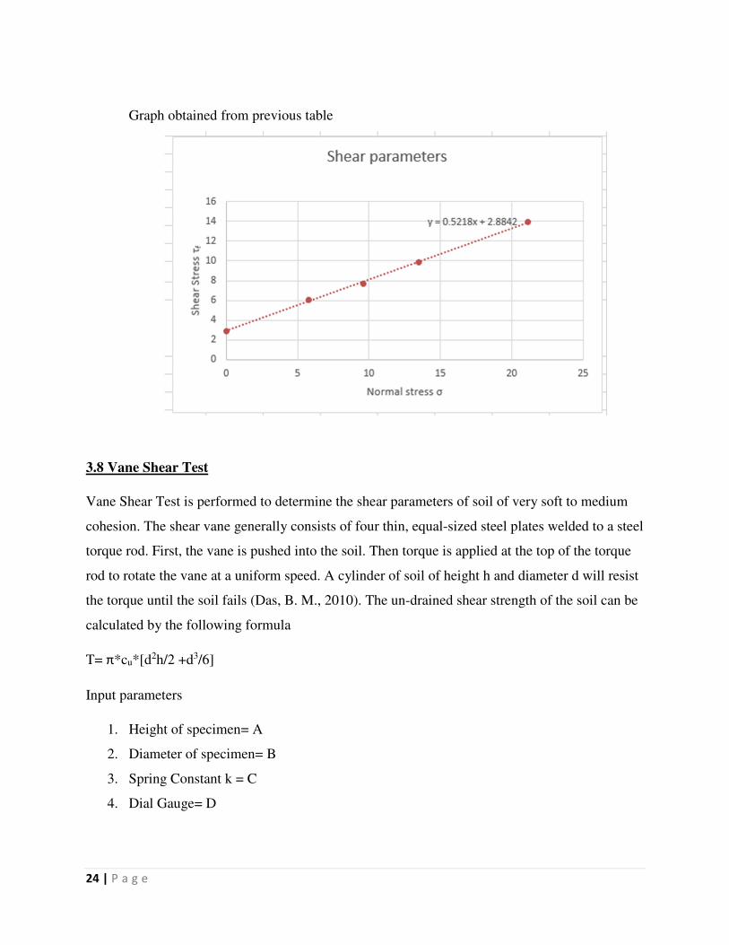
Excel spread sheet developed for direct shear( table 3.7)

24 | P a g e

Graph obtained from previous table

3.8 Vane Shear Test

Vane Shear Test is performed to determine the shear parameters of soil of very soft to medium

cohesion. The shear vane generally consists of four thin, equal-sized steel plates welded to a steel

torque rod. First, the vane is pushed into the soil. Then torque is applied at the top of the torque

rod to rotate the vane at a uniform speed. A cylinder of soil of height h and diameter d will resist

the torque until the soil fails (Das, B. M., 2010). The un-drained shear strength of the soil can be

calculated by the following formula

T= π*cu*[d2h/2 +d3/6]

Input parameters

1. Height of specimen= A

2. Diameter of specimen= B

3. Spring Constant k = C

4. Dial Gauge= D

25 | P a g e

Output parameters:

1. Volume of specimen = π* B2A/4=E

2. Final Torque = D*C=F

3. Shear strength = F/(π)[B2A/2 + B3/6]

Excel spread sheet developed for vein shear test( Table 3.8)

3.9 GRAIN SIZE DISTRIBUTION BY SIEVE ANALYSIS AND HYDROMETER

ANALYSIS

Sieve Analysis:

Sieve analysis consists of passing the soil sample through a set of sieves that have progressively

smaller openings. The size of the sieves are mentioned in Indian Standard codes IS-2720(part 4),

1985

Before passing the soil through the sieves the soil should be thoroughly broken from lumps and

then passed. After the passing of soil, the mass ret ined should be cumulated and then formulated

in a tabular format.

26 | P a g e

Snap shot of the spread sheet developed for sieve analysis (Table 3.9 a)

The residual mass that is the finer particles which pass through the sieves are collected and tested

for hydrometer analysis.

Hydrometer analysis: Hydrometer analysis is based on the principle of sedimentation of soil grains

in water. When a soil specimen is dispersed in water, the particles settle at different velocities,

depending on their shape, size, weight, and the viscosity of the water.

Initial mass 1000 gm

PARTICLE PARTICLE MASS % CUM % %

SIZE (mic) SIZE (mm) RETAINE

D(g)

RETAINE

D

RETAINE

D

FINER

50000.00 50.00 0.00 0.00 0.00 100.00

40000.00 40.00 0.00 0.00 0.00 100.00

20000.00 20.00 0.00 0.00 0.00 100.00

10000.00 10.00 0.00 0.00 0.00 100.00

6250.00 6.25 0.00 0.00 0.00 100.00

4750.00 4.75 22.00 2.20 2.20 97.80

2000.00 2.00 21.00 2.10 4.30 95.70

1000.00 1.00 22.00 2.20 6.50 93.50

425.00 0.43 134.00 13.40 19.90 80.10

212.00 0.21 289.00 28.90 48.80 51.20

150.00 0.15 135.00 13.50 62.30 37.70

75.00 0.08 144.00 14.40 76.70 23.30

767.00 gm

Residual 233.00 gm

27 | P a g e

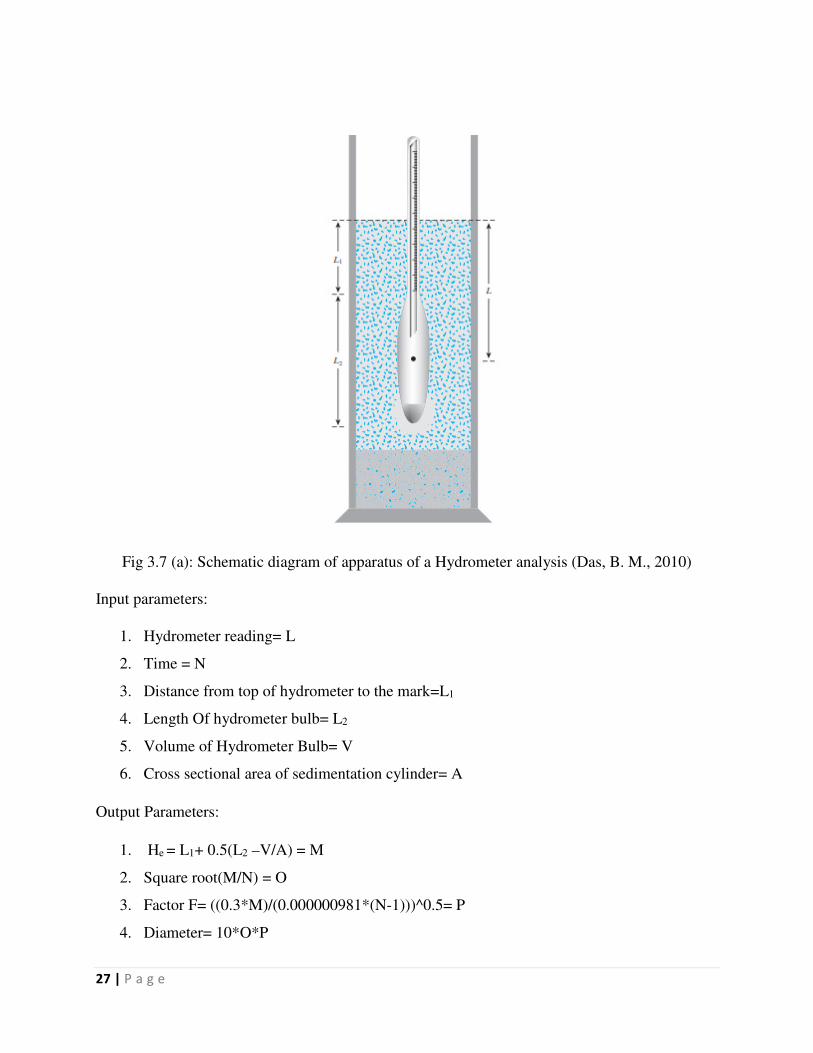
Fig 3.7 (a): Schematic diagram of apparatus of a Hydrometer analysis (Das, B. M., 2010)

Input parameters:

1. Hydrometer reading= L

2. Time = N

3. Distance from top of hydrometer to the mark=L1

4. Length Of hydrometer bulb= L2

5. Volume of Hydrometer Bulb= V

6. Cross sectional area of sedimentation cylinder= A

Output Parameters:

1. He = L1+ 0.5(L2 –V/A) = M

2. Square root(M/N) = O

3. Factor F= ((0.3*M)/(0.000000981*(N-1)))^0.5= P

4. Diameter= 10*O*P

28 | P a g e

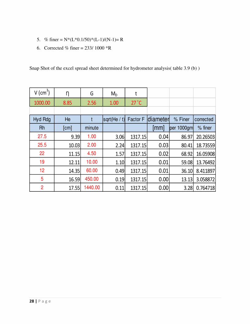
5. % finer = N*(L*0.1/50)*(L-1)/(N-1)= R

6. Corrected % finer = 233/ 1000 *R

Snap Shot of the excel spread sheet determined for hydrometer analysis( table 3.9 (b) )

V (cm3) Ƞ G MD t

1000.00 8.85 2.56 1.00 27 ˚C

Hyd Rdg He t sqrt(He / t) Factor F diameter % Finer corrected

Rh [cm] minute [mm] per 1000gm % finer

27.5 9.39 1.00 3.06 1317.15 0.04 86.97 20.26503

25.5 10.03 2.00 2.24 1317.15 0.03 80.41 18.73559

22 11.15 4.50 1.57 1317.15 0.02 68.92 16.05908

19 12.11 10.00 1.10 1317.15 0.01 59.08 13.76492

12 14.35 60.00 0.49 1317.15 0.01 36.10 8.411897

5 16.59 450.00 0.19 1317.15 0.00 13.13 3.058872

2 17.55 1440.00 0.11 1317.15 0.00 3.28 0.764718

29 | P a g e

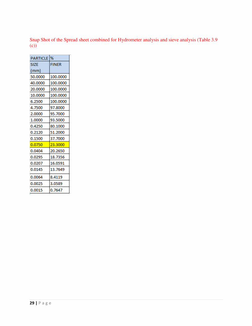
Snap Shot of the Spread sheet combined for Hydrometer analysis and sieve analysis (Table 3.9

(c))

30 | P a g e

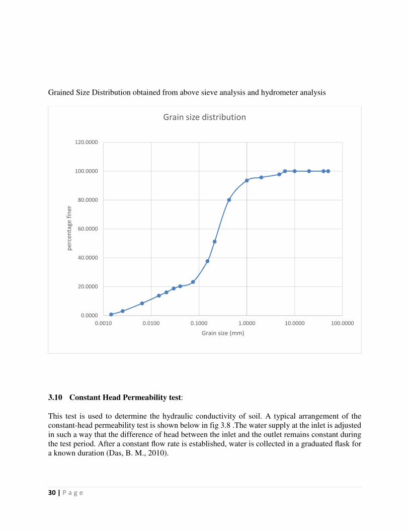
Grained Size Distribution obtained from above sieve analysis and hydrometer analysis

3.10 Constant Head Permeability test:

This test is used to determine the hydraulic conductivity of soil. A typical arrangement of the

constant-head permeability test is shown below in fig 3.8 .The water supply at the inlet is adjusted

in such a way that the difference of head between the inlet and the outlet remains constant during

the test period. After a constant flow rate is established, water is collected in a graduated flask for

a known duration (Das, B. M., 2010).

0.0000

20.0000

40.0000

60.0000

80.0000

100.0000

120.0000

0.0010 0.0100 0.1000 1.0000 10.0000 100.0000

pe

rce

nta

ge

fin

er

Grain size (mm)

Grain size distribution

31 | P a g e

The volume of water collected is calculated by V= Avt

Where t= duration of water collection.

A= area of cross section of the soil specimen

Input parameters

1. Head Difference= B

2. Volume= D

3. Time= E

Output parameters:

1. Hydraulic gradient i= B/Length = C

2. Velocity= D/Area*t= G

3. K=co-efficient of permeability= G/C

32 | P a g e

Snapshot of the excel Spread sheet determined for Constant head permeability test (Table

3.10)

Graph Obtained from the above input is

33 | P a g e

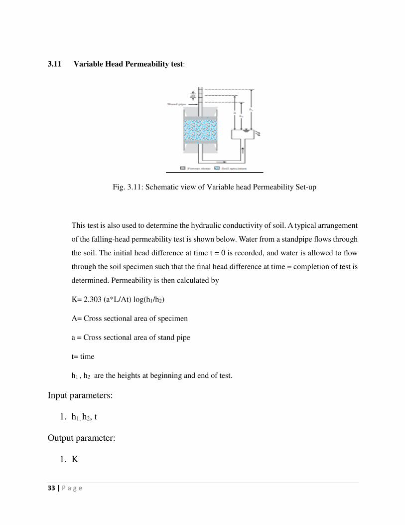
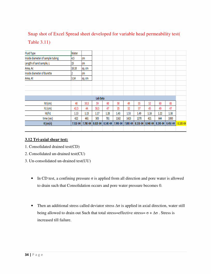
3.11 Variable Head Permeability test:

Fig. 3.11: Schematic view of Variable head Permeability Set-up

This test is also used to determine the hydraulic conductivity of soil. A typical arrangement

of the falling-head permeability test is shown below. Water from a standpipe flows through

the soil. The initial head difference at time t = 0 is recorded, and water is allowed to flow

through the soil specimen such that the final head difference at time = completion of test is

determined. Permeability is then calculated by

K= 2.303 (a*L/At) log(h1/h2)

A= Cross sectional area of specimen

a = Cross sectional area of stand pipe

t= time

h1 , h2 are the heights at beginning and end of test.

Input parameters:

1. h1, h2, t

Output parameter:

1. K

34 | P a g e

Snap shot of Excel Spread sheet developed for variable head permeability test(

Table 3.11)

3.12 Tri-axial shear test:

1. Consolidated drained test(CD)

2. Consolidated un-drained test(CU)

3. Un-consolidated un-drained test(UU)

• In CD test, a confining pressure σ is applied from all direction and pore water is allowed

to drain such that Consolidation occurs and pore water pressure becomes 0.

• Then an additional stress called deviator stress ∆σ is applied in axial direction, water still

being allowed to drain out Such that total stress=effective stress= σ + ∆σ . Stress is

increased till failure.

35 | P a g e

• In CU test, the pore water pressure at 2nd stage is not allowed to dissipate, thereby

making effective stress=

total stress-pore water pressure= σ + ∆σ -∆u= σ + ∆σ - uf

• In UU test, drainage is not allowed in both the stages, thereby effective stress=total-pore

water pressure = (σ + ∆σ)-∆u= σ + ∆σ –(uf-ui)

*minor stress is obtained by putting ∆σ =0.

Input parameters:

Confining stress, confining stress+ deviator stress

Output parameters:

Shear parameters c and phi.

Algorithm used to develop the excel spread sheet

Step 1: the σi=confining stress and σf=final stress after deviator stress is applied is obtained

according to the type of tri-axial test.

Step2: center and radius of the Mohr coulomb failure is calculated by (σf+σi )/2 and (σf-σi )/2

Step3: The half circle is then divided into 1800 strips from ϴ=[0,π] with increment= π/1800

Step 4: ϴ=0+ϴi where i=0 to 1800

Step 5: xi=center +radius*cos ϴi are found for all 1800 points.

Step6: yi=radius*sin ϴi are found for all 1800 points.

Step 7: m=slope=tan(0.5* π- ϴi ) is calculated for all points

Step 8: c=intercept=: yi+m*(0-xi) is calculated.

36 | P a g e

For two different mohr circle, let us take 2 different input parameters, and thereby we have the

coordinates of 1800 points on the circle for the 2 circles.

At failure, c is equal for both circles.

Step 9: (c1-c2)min is found for all 1800 points and assign (c1-c2)min =c

Step 10: if (c1-c2)=c, then c=c, else 0.

Step 11: if c=0, ɸ=slope=o, else Ф=arctan(mi)

37 | P a g e

Calculation spread sheet of triaxial shear test( Table 3.12 )

38 | P a g e

Mohr coulomb failure envelope (graph of σ vs τ)

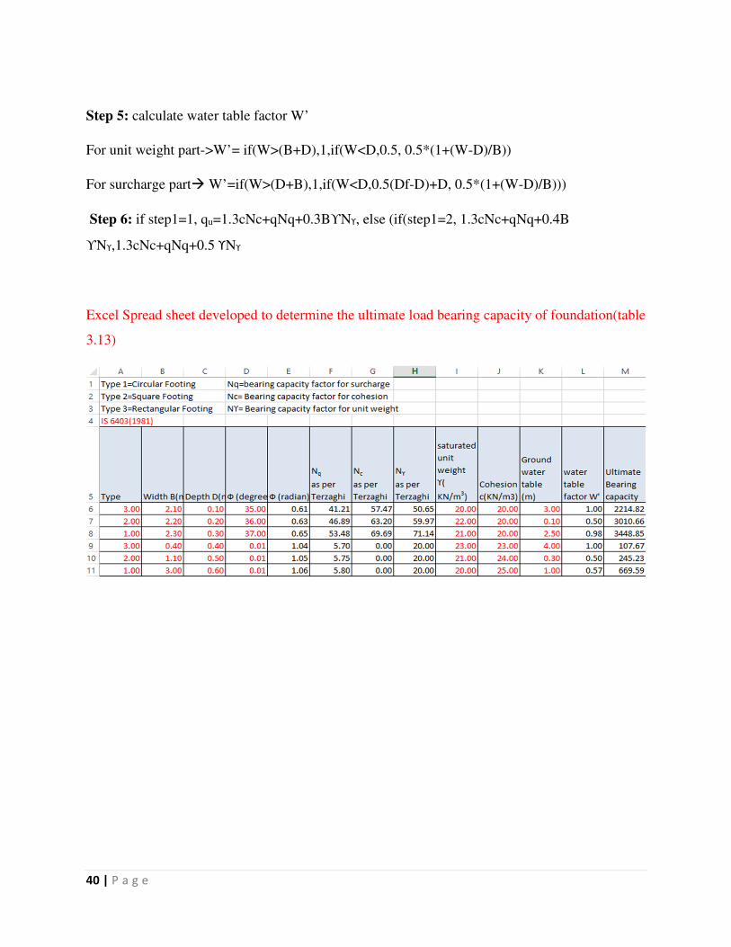
3.11 Load bearing capacity of shallow foundation:

Foundation is the lowest part of a structure. It transfers the load of the structure to the soil

on which it is rests. A good foundation transfers the load throughout the soil evenly so

that failure does not occur. Overstressing the soil can result in either excessive settlement

or shear failure of the soil. Hence, Bearing capacity of soil is important for engineers who

design the foundation.

Input parameters:

1. Type of foundation

2. Width of foundation

3. Depth of foundation

4. Angle of friction , phi

5. Saturated unit weight of soil

6. Cohesion of soil

39 | P a g e

7. Water table depth

Formula used:

1. Terzaghi equation:

Qu= qc + qq + qϒ

Where qc= cNc

qq= qNq

qϒ= kBϒNϒ, k=0.3 for circular, 0.4 for square and 0.5 for rectangular

2

tan24

32

245cos2

+

=

−

φ

φφπ

eN q

( ) φcot1−= qc NN

( ) ( )2tancot18.1 φφγ −≈ qNN

2. For water table

W’= water table factor is given by

For unit weight part->W’= if(W>(B+D),1,if(W<D,0.5, 0.5*(1+(W-D)/B))

For surcharge part� W’=if(W>(D+B),1,if(W<D,0.5(Df-D)+D, 0.5*(1+(W-D)/B)))

Algorithm used

Step1: let us assign the value 1,2,3 as

1=Circular Footing

2=Square Footing

3=Rectangular Footing

Step2: enter input parameters (W)width, (D)depth and (ɸ)shear parameter.

Step 3: Calculate Nc, Nq and Nϒ as per terzaghi’s equations

Step 4: enter the input parameters unit weight(ϒ), water table (w), cohesion ( c )

40 | P a g e

Step 5: calculate water table factor W’

For unit weight part->W’= if(W>(B+D),1,if(W<D,0.5, 0.5*(1+(W-D)/B))

For surcharge part� W’=if(W>(D+B),1,if(W<D,0.5(Df-D)+D, 0.5*(1+(W-D)/B)))

Step 6: if step1=1, qu=1.3cNc+qNq+0.3BϒNϒ, else (if(step1=2, 1.3cNc+qNq+0.4B

ϒNϒ,1.3cNc+qNq+0.5 ϒNϒ

Excel Spread sheet developed to determine the ultimate load bearing capacity of foundation(table

3.13)

41 | P a g e

Conclusions

Based on the theory and procedure of some commonly used geotechnical laboratory test, an excel

spreadsheet has been developed and the conclusions are the following:

� An honest effort is being made to determine the output of some geotechnical engineering

laboratory experiments in an excel spreadsheet in a comprehensive manner.

� The results are found to be consistent with previously obtained data

42 | P a g e

REFERENCE

1. Das, B.M., (2010)“ Principles of geotechnical engineering” 7th edition, Cengage Learning

2. Punmia, B.C., Jain, A.K., Jain. A.K. (2005) “Soil Mechanics and foundations” 16th edition,

laxmi Publication.

3. Indian Standard Codes for geotechnical laboratory experiments.