arX

iv:1

705.

0305

0v1

[st

at.A

P] 8

May

201

7

Development of an Accelerated Test Methodology to the

Predict Service Life of Polymeric Materials Subject to

Outdoor Weathering

Yuanyuan Duan1, Yili Hong1, William Q. Meeker2,

Deborah L. Stanley3, and Xiaohong Gu3

1Department of Statistics, Virginia Tech, Blacksburg, VA 24061

2Department of Statistics, Iowa State University, Ames, IA 50011

3Engineering Laboratory, National Institute of Standards and Technology,

Gaithersburg, MD 20899

May 10, 2017

Abstract

Service life prediction is of great importance to manufacturers of coatings and other

polymeric materials. Photodegradation, driven primarily by ultraviolet (UV) radiation,

is the primary cause of failure for organic paints and coatings, as well as many other

products made from polymeric materials exposed to sunlight. Traditional methods of

service life prediction involve the use of outdoor exposure in harsh UV environments

(e.g., Florida and Arizona). Such tests, however, require too much time (generally

many years) to do an evaluation. Non-scientific attempts to simply “speed up the

clock” result in incorrect predictions. This paper describes the statistical methods

that were developed for a scientifically-based approach to using laboratory acceler-

ated tests to produce timely predictions of outdoor service life. The approach involves

careful experimentation and identifying a physics/chemistry-motivated model that will

adequately describe photodegradation paths of polymeric materials. The model incor-

porates the effects of explanatory variables UV spectrum, UV intensity, temperature,

and humidity. We use a nonlinear mixed-effects model to describe the sample paths.

The methods are illustrated with accelerated laboratory test data for a model epoxy

coating. The validity of the methodology is checked by extending our model to allow for

dynamic covariates and comparing predictions with specimens that were exposed in an

outdoor environment where the explanatory variables are uncontrolled but recorded.

Key Words: Degradation, Photodegradation, Nonlinear model, Random effects,

Reliability, UV exposure, Weathering.

1

1 Introduction

1.1 Background and Motivation

Polymeric materials are widely used in many products such as paints, coatings, and com-

ponents in systems such as photovoltaic power generation equipment (e.g., encapsulant and

backsheet). Photodegradation caused by ultraviolet (UV) radiation is the primary cause of

failure for paints and coatings, as well as many other products made from polymeric materi-

als that are exposed to sunlight. Other environmental variables including temperature and

humidity can also affect degradation rates. When a new product that will be subjected to

outdoor weathering is developed, it is necessary to assess the product’s service life. As an

example, for paints and coatings, the traditional method of service life prediction involves

sending perhaps ten coated panels to Florida (where it is sunny and humid) and another ten

panels to Arizona (where it is sunny and dry). Then every six months one panel is returned

from each exposure location for detailed evaluation (e.g., to quantify chemical and physical

changes over time). If the amount of degradation is sufficiently small after, say, five years,

the service life is deemed to satisfactorily long.

The problem with the traditional method of service life prediction is that it takes too long

to obtain the needed assessment. For many decades, accelerated tests (e.g., Nelson 1990)

have been used successfully to assess the lifetime of products and components in environments

that do not involve UV exposure. Accelerated tests for photodegradation are, however, more

complicated. Non-scientific approaches to achieve acceleration of the degradation process by

simply “speeding up the clock” in laboratory testing led to incorrect predictions. It is believed

that the efforts failed for a combination of reasons including that UV lamps do not have the

same spectral irradiance distribution as the sun and that varying all experimental factors

simultaneously (the opposite of what would be done in a carefully designed experiment) does

not provide useful information for modeling and prediction.

Scientists at the U.S. National Institute of Standards and Technology (NIST), in collab-

oration with scientists and engineers from companies and other organizations, conducted a

multi-year research program to develop a scientifically-based laboratory accelerated testing

methodology that could be used to predict the service life of polymeric materials subjected

to outdoor weathering. The purpose of this paper is to describe the statistical methods that

were used for physical/chemical modeling and to compute predictions of outdoor service life,

based on the laboratory accelerated test. The methods were validated by comparing the pre-

dictions with specimens that were subjected to outdoor exposure where dynamic explanatory

variables (i.e., time-varying covariates) although not controlled, were recorded.

The laboratory accelerated weathering tests were conducted using the NIST SPHERE

(Simulated Photodegradation via High Energy Radiant Exposure), a device in which spectral

2

UV wavelength, UV spectral intensity, temperature, and relative humidity (RH) can be con-

trolled over time. Also, outdoor-exposure experiments were conducted on the roof of a NIST

building in Maryland over different time periods. Both sets of experiments used a model

epoxy coating. Chemical degradation was measured on both the laboratory accelerated test

specimens and the outdoor-exposed specimens every few days using Fourier transform in-

frared (FTIR) spectroscopy. Longitudinal information on ambient temperature, RH, and

the solar intensity and spectrum for outdoor-exposed specimens were carefully recorded at

12-minute intervals over the period of outdoor exposure.

1.2 A General Framework for Degradation Prediction

This section summarizes the major steps in the general framework for accelerated pho-

todegradation testing of polymeric materials that are subject to outdoor weathering.

1. Use the accelerated test data and knowledge of the physics and chemistry of the degra-

dation process to help identify the functional forms for the experimental variables as they

relate to the degradation path model.

2. Use the identified functional forms and the accelerated test data to build a degradation

path model linking the sample degradation paths and the experimental variables.

3. Use the identified model to generate predictions of degradation for a given covariate

histories.

4. To verify the effectiveness of the accelerated test methodology, compare predictions,

based on the accelerated test degradation data and model, with observed degradation paths for

outdoor-exposed specimens.

5. Use prediction intervals to quantify the statistical uncertainties associated with the

outdoor degradation predictions.

In summary, the presented modeling approach advocates the strategy of combining phys-

ical/chemical knowledge and accelerated test data to build a model that can predict field

performance.

1.3 Related Literature and Contribution of This Work

Traditional life tests generally require a long time to obtain a substantial number of failures

because modern products are designed to last a long time. To overcome the time constraints

of life tests, degradation data provide quantitative measurements and thus more informa-

tion than failure data. Lu and Meeker (1993), and Meeker, Hong, and Escobar (2011) give

examples of models and analyses of degradation data. To speed up the degradation pro-

cess and provide information in a more timely manner, accelerated degradation tests are

commonly used (e.g., Chapter 12 of Nelson 1990, Chapter 21 of Meeker and Escobar 1998,

3

and Meeker, Escobar, and Lu 1998). The use of degradation data in accelerated tests pro-

vides more credible and precise reliability estimates and a firmer basis for extrapolation

at normal use conditions. Potential accelerating variables include the use rate or aging

rate of a product, exposure intensity, voltage stress, temperature, humidity, etc. (e.g.,

Escobar and Meeker 2006). Combinations of these accelerating variables are sometimes used.

For products and systems in the field, the degradation process usually depends on dy-

namic environmental covariates. Dynamic data collection is becoming much easier with

modern sensor technology, motivating the modeling of the effect of dynamic covariates. For

example, Hahn and Doganaksoy (2008) described sensors recording dynamic covariates such

as oil pressure and oil/water temperature in locomotive engines and how the information

could be used to diagnose system faults. Spurgeon et al. (2005) described an automatic sys-

tem that can monitor dissolved gas in the insulating oil in high-voltage power transformers

to detect the occurrence of arcing that could, if not corrected, lead to a catastrophic failure.

Degradation processes are often affected by dynamic covariates but it is challenging to

incorporate such information into a degradation-process model. The cumulative damage

model has been used to describe the effect that dynamic covariates have on degradation and

failure-time processes (e.g., Nelson 1990, Subramanian, Reifsnider, and Stinchcomb 1995,

Bagdonavicius and Nikulin 2001, Vaca-Trigo and Meeker 2009, Hong and Meeker 2010, and

Hong and Meeker 2011). Hong et al. (2015), and Xu et al. (2016) use the NIST outdoor-

exposure data to build predictive models for degradation. One problem with those ap-

proaches is that there is no acceleration and the evaluation of service life, for many products,

would take too long.

It takes a long time to observe the actual service life performance of new products and

systems. For example, when new coatings are being developed, there is a need to have exten-

sive outdoor exposure to characterize service life performance. Depending on the product,

such outdoor exposures could take many years or even decades (Martin et al. 1996). Also,

the outdoor exposure conditions are complicated, due to the joint effects of multiple dy-

namic covariates. Laboratory accelerated tests can be conducted over much shorter periods

of time. With knowledge of the failure mechanisms and proper scientific modeling of data

from a well-designed experiment, it is possible to predict outdoor service life performance. It

will be practically useful if the laboratory accelerated test data and the outdoor performance

data can be linked. Gu et al. (2009) described three potential approaches to link laboratory

accelerated degradation test data with outdoor-exposure data for a coating system.

• An approach based on chemical concentration ratios,

• A heuristic approach, and

• An approach based on a predictive model.

In a preliminary report of the NIST experimental program, Vaca-Trigo and Meeker (2009)

described a predictive model to link the NIST laboratory accelerated test data and outdoor-

4

exposure data. They used a nonlinear model for the accelerated test data and a cumulative

damage model to predict the outdoor-exposure data. In this paper we extend this previ-

ous work to provide a better, more scientifically justified model for the explanatory-variable

effects and the different sources of variability. We also provide improved methods to make

service life predictions and to quantify prediction error, making it possible to quantitatively

compare the predictions with the outdoor-exposure data.

More specifically, in this paper we extend the work in Vaca-Trigo and Meeker (2009)

by using a sophisticated nonlinear mixed-effects model with careful physically-motivated

modeling of the effects of the accelerating variables on the sample degradation paths. This

improved model provides enhanced prediction performance and the ability to quantify predic-

tion uncertainty with prediction intervals. More generally, this paper provides the following

advances.

• We propose and develop a general modeling and prediction framework for accelerated

photodegradation testing of polymeric materials. The methodology framework is illustrated

by the data collected from a model epoxy (which would tend to degrade rapidly—providing

further acceleration) but it can also be used to predict the degradation of other materials

such as ethylene-vinyl acetate (EVA) and polyethylene terephthalate (PET) and materials

containing UV protection (similar to sunscreens that humans use to protect their skin from

harmful UV radiation).

• The proposed stage-wise modeling method provides a means to combine scientific knowl-

edge of the degradation process with experimental data to identify the functional form of

each accelerating variable in the degradation path model. This general methodology will be

useful for other kinds of accelerated degradation studies.

• A prediction procedure based on a cumulative damage model is developed and predic-

tion uncertainties are quantified with prediction intervals.

1.4 Overview

The rest of this paper is organized as follows. Section 2 describes the laboratory accelerated

test and the outdoor-exposure experiments and provides notation for the data. Section 3

describes the nonlinear mixed-effects model and defines total effective dosage. Section 4 uses

the laboratory accelerated test data to compute estimates of a categorical-effects model,

providing information about the functional forms of the experimental variables needed to

identify a model relating photodegradation to the experimental variables. Section 5 uses

model parameter estimates from the laboratory accelerated test data and a cumulative dam-

age model to predict outdoor-exposure degradation and compares the predictions with actual

outdoor-exposure degradation paths. A comparison is also done for several different mod-

els in terms of model fitting and prediction accuracy. Section 6 contains conclusions and

5

discussion of areas for future research.

2 Photodegradation Time Scale and Data

2.1 Choice of a Time Scale

As described on page 4 of Cox and Oakes (1984) and page 18 of Meeker and Escobar (1998),

when conducting any kind of failure-time study, it is important to carefully consider the

time scale to be used. For example, roller bearing life would most reasonably be measured

in terms of something proportional to the number of revolutions. If the bearing is installed

in an automobile, that information might not be available and so the number of miles driven

would be a useful surrogate. For a rubber seal or an adhesive in a controlled environment

and no UV exposure, something proportional to real time (e.g., months in service) would

be appropriate. For a coating subjected to UV exposure, the scientifically appropriate time

scale would be proportional to the number of photons that get absorbed into the coating,

taking into account that shorter wavelength photons are more energetic (and thus have a

higher probability to cause damage). For those who study photodegradation, such a measure

is called UV dosage, as will be described in detail in subsequent sections of this paper.

2.2 Laboratory Accelerated Test Experiments and Data

The light source for the laboratory accelerated test experiments is high-intensity UV lamps.

The spectral irradiance of the lamps is a function of wavelength λ, which gives the power

density at a particular wavelength λ. The spectral irradiance of the UV lamps in the NIST

SPHERE is illustrated in Figure 1. Specifically, the irradiance is defined as the power of the

electromagnetic radiation per unit area incident on a surface.

The effect of UV radiation on degradation depends on both the UV spectrum and UV

intensity. UV radiation with shorter wavelengths tend to have higher energy per photon,

thus causing more damage to the material when compared with UV radiation with longer

wavelengths. Also, for the UV with the same wavelength, higher UV intensity (means more

photons per time unit) tends to cause more damage than lower intensity. To study the effect

of UV spectrum and UV intensity, the spectral irradiance of the lamps was modified and

controlled by bandpass (BP) and neutral density (ND) filters. BP filters pass only UV with

wavelengths over a particular range. For example, the 306 nanometer (nm) BP filter has a

nominal center wavelength of 306 nm and full-width-half maximum values of ±3 nm. The

four BP filters used in the experiments have nominal center wavelengths of 306 nm, 326 nm,

353 nm, and 452 nm.

ND filters control the intensity of the UV radiation without affecting the shape of the

6

300 350 400 450 500 550

0

1

2

3

4

5

6

Wavelength (nm)

Lam

p S

pect

ral I

rrad

ianc

e

Figure 1: Plot of the laboratory accelerated test lamp spectral irradiance distribution.

300 350 400 450 500

0

20

40

60

80

100Neutral Density 10%

Wavelength (nm)

Bandpass Filter 306Bandpass Filter 326Bandpass Filter 353Bandpass Filter 452

300 350 400 450 500

0

20

40

60

80

100Neutral Density 40%

Wavelength (nm)

300 350 400 450 500

0

20

40

60

80

100Neutral Density 60%

Wavelength (nm)

300 350 400 450 500

0

20

40

60

80

100Neutral Density 100%

Wavelength (nm)

Figure 2: Illustration of the combinations of the BP and ND filters. The y-axis shows the

percentage of photons passing through the combinations of filters.

7

Table 1: Laboratory accelerated test setup, showing the BP filters, ND filters, and levels of

temperature and RH.

BP filter306 nm (±3 nm), 326 nm (±6 nm),353 nm (±21 nm), 452 nm (±79 nm)

ND filter 10%, 40%, 60%, 100%Temperature 25◦C, 35◦C, 45◦C, 55◦C

RH 0%, 25%, 50%, 75%

Table 2: Summary of the 80 experimental combinations of BP and ND filters and temper-

ature and RH levels. An empty cell implies that no experiments were done for the corre-

sponding combination of temperature and RH. 4× 4 implies that experiments were done for

all of the 16 combinations of the BP and ND filters at the corresponding temperature and

RH combination. 4 × 1 implies that experiments were done for all four BP filters and the

100% ND filters for the corresponding temperature and RH combination.

❍❍❍❍❍❍❍❍

Temp

RH0% 25% 50% 75%

25 4× 435 4× 4 4× 1 4× 145 4× 1 4× 1 4× 455 4× 4

UV spectrum. For example, a 10% ND filter (nominally) passes 10% of the UV photons

at any wavelength. The four ND filters used in the experiments are 10%, 40%, 60% and

100% (actually, a 100% ND would use no ND filter). As an illustration, Figure 2 shows all

combinations of the 16 BP and ND filters.

The laboratory accelerated test experiments also have other controlled environmental

factors: temperature and RH. Table 1 gives a summary of the experimental factors for the

laboratory accelerated degradation experiment. The temperature levels were 25◦C, 35◦C,

45◦C, and 55◦C. The RH levels were 0%, 25%, 50%, and 75%. The laboratory acceler-

ated test data contain a total of 80 combinations of the experimental factors. Due to time

and funding constraints, not all combinations of the four experimental factors were run in

the experiments. Table 2 summarizes the 80 experiment combinations of the BP and ND

filters and temperature and RH levels. There were four replicates for most of the experi-

mental factor-level combinations. A total of 319 specimens were exposed in the laboratory

accelerated test experiments.

Damage to the material, which is used as an indication for degradation, was measured

by Fourier transform infrared (FTIR) spectroscopy. An FTIR spectrometer provides an

8

Figure 3: Illustration of FTIR spectrum of the model epoxy used in the NIST experiments.

infrared spectrum of absorption or emission of a material. In particular, special structures of

compounds absorb the infrared energy at different wavelengths, which results in peaks in the

FTIR spectra. The locations of the FTIR peaks correspond to unique chemical structures

and thus can be used to identify the relative concentration of different compounds. The

height of a peak is proportional to the concentration of a particular compound or structure.

The time intervals between the FTIR measurements in the accelerated test were typically

on the order of a few days.

Figure 3 gives an illustration of FTIR peaks for a particular specimen at one point in

time. Our modeling focuses on intensity changes at wavenumber 1250 cm−1, which cor-

respond to C-O stretching of aryl ether. Other peaks that were recorded as potentially

useful responses include 1510 cm−1 (benzene ring stretching), 1658 cm−1 (C=O stretching

of oxidation products), and 2925 cm−1 (CH2 stretching) (e.g., see Bellinger and Verdu 1984,

Bellinger and Verdu 1985, Rabek 1995, and Kelleher and Gesner 1969).

As an example of the degradation data collected in the laboratory accelerated test experi-

ments, Figure 4 shows the degradation paths for FTIR wavenumber 1250 cm−1 for specimens

with 10%, 40%, 60% and 100% ND filters, the BP filter centered at 353 nm, temperature

35◦C, and 0% RH. For this wavenumber, the degradation paths are decreasing (i.e., the

amount of C-O stretching of aryl ether was decreasing). As expected, the degradation rates

were higher for the ND filters passing larger percentages of UV photons. For the groups of

two to four specimens exposed to the same conditions (and at the same time and in the same

chamber), there is some specimen-to-specimen variability.

To use a degradation model to make inferences about failure times, it is necessary to have

a definition of failure. When dealing with soft failures (as is commonly done in degradation

9

0 50 100 150 200 250

−0.8

−0.6

−0.4

−0.2

0.0

Days Since the First Measurement

Dam

age

Am

ount

s

Netural Density=10Netural Density=40Netural Density=60Netural Density=100Failure Threshold

Figure 4: Degradation paths for specimens with 10%, 40%, 60% and 100% ND filters, the

353 nm BP filter, temperature at 35◦C, and 0% RH.

applications), such definitions generally have a subjective element (e.g., at what point in

loss of gloss of a coating do we have a failure), but such decisions are typically made in

a purposeful manner with great care (e.g., using customer survey information to assess

perception of gloss loss). These ideas relating degradation modeling to the estimation of

service life are widely used in applications of degradation data modeling (e.g., the light

output of lasers and LEDs, corrosion of pipelines, and growth of cracks in structures). During

the NIST experimental program, physical measurements of gloss loss were also taken and

correlated with the FTIR chemical degradation measurements. One reason that we choose

to use the wavenumber 1250 cm−1 as our response is that it correlated best with gloss loss

of the model epoxy used in the NIST experiments. As shown by the horizontal lines in

Figures 4 and 5, a damage level of −0.40 was used as the failure definition.

2.3 Outdoor-Exposure Experiments and Data

The UV exposure for the outdoor-exposure specimens is from the sun. There were 53 speci-

mens in the outdoor-exposure experiments and they were exposed over different time intervals

during a three-year period. The UV spectral irradiance, temperature, and RH are, of course,

uncontrolled outside, but were recorded at 12-minute intervals. For the outdoor-exposure

specimens, the UV, temperature, and RH are dynamic covariates. The measurements of

10

0 50 100 150

−0.5

−0.4

−0.3

−0.2

−0.1

0.0

Days Since the First Measurement

Dam

age

Am

ount

s

Failure Threshold

Figure 5: Plots of the degradation paths as a function of the days since the first measurement

for a representative subset of 12 outdoor-exposed specimens.

degradation were taken every three to four days, similar to the accelerated test specimens.

We continue to focus on chemical changes at wavenumber 1250 cm−1. Note, however, that

we used the laboratory accelerated test data for model fitting. The data from the outdoor-

exposed specimens are used only for validating the accelerated test methodology.

We also want to point out the interesting difference between the laboratory accelerated

test data and outdoor-exposure data. The data shown in Figure 4 were collected in laboratory

accelerated tests in which the UV, temperature, and RH are controlled to be constant over

time. All of the sample paths have the same shape. Figure 5, on the other hand, shows

the sample degradation paths as a function of the days since the beginning of exposure for

a representative subset of 12 specimens that were exposed outdoors at different times. The

sample degradation paths have different shapes, depending on the time of the year that the

specimens were being exposed. The variability in the shapes of degradation paths for the

outdoor-exposure data is due to variability in the dynamic covariate time series.

To further illustrate and understand the outdoor-exposure degradation-path patterns,

Figure 6(a) shows the degradation path for a particular outdoor-exposed specimen as a

function of the calendar time. Figures 6(b), 6(c), and 6(d) show the dynamic covariates

corresponding to the particular degradation path in Figure 6(a). From Figure 6(d), we can

see that the UV intensity is low during the late fall and winter months, corresponding to a

smaller slope in the degradation path, while the UV is stronger for the months of March and

11

April, corresponding to a larger slope in the degradation path.

2.4 Notation

Here we introduce notation for the data. The degradation (damage) measurement for spec-

imen i is the change (relative the value at the beginning of exposure) in the FTIR peak

at 1250 cm−1 at time tij and for the laboratory accelerated test data is denoted by yi(tij),

i = 1, . . . , n, j = 1, . . . , mi. Here, n is the total number of laboratory accelerated test speci-

mens and mi is the number of time points where the degradation measurements were taken

for specimen i. The last observation time for specimen i is denoted by ti = timi.

For the laboratory accelerated test data, the UV radiation is quantified by the cumula-

tive dosage Di(τil) at time τil. (Note that the cumulative dosage values were reported at

times that differ from the times at which the degradation measurements were taken.) The

cumulative dosage is proportional to the total number of photons that were absorbed by

specimen i across all wavelengths between time 0 and τil. Here, i = 1, . . . , n, l = 1, . . . , ni,

where ni is the number of time points at which the total dosage was recorded for specimen i.

For the laboratory accelerated test specimens, the experimental factors are held constant

at specified levels over time. We let BPi, NDi, Tempi, and RHi be the BP filter, ND filter,

temperature, and RH levels, respectively, for specimen i. In summary, the laboratory accel-

erated test data are {yi(tij), Di(τil),BPi,NDi,Tempi,RHi} for i = 1, . . . , n, j = 1, . . . , mi,

and l = 1, . . . , ni.

For the outdoor-exposure data, we use subscript k to index the exposed specimens. The

degradation measurement at time tkj is denoted by yk(tkj), k = 1, . . . , q, j = 1, . . . , mk for

specimen k. Here q is the number of outdoor-exposure specimens. The recorded ambient

temperature and RH for specimen k at time τkl are denoted by Tempk(τkl) and RHk(τkl),

l = 1, . . . , nk, respectively. For the UV radiation, dosage was recorded for each 12-minute

interval and each 2 nm wavelength interval between 300 nm and 532 nm. We denote the UV

dosage for outdoor-exposure specimen k at time τkl and wavelength interval λ by Dk(τkl, λ).

An example of Dk(τkl, λ) data is shown in Figure 6(d). In summary, the outdoor-exposure

data are {yk(tkj), Dk(τkl, λ),Tempk(τkl),RHk(τkl)} for k = 1, . . . , q, l = 1, . . . , nk, and j =

1, . . . , mk.

2.5 Data Cleaning

The data required cleaning before the analysis. For a certain number of specimens in the

laboratory accelerated test data, the degradation paths show two segments instead of con-

tinuous curves. This was believed to have been caused by a specimen-preparation problem,

so those specimens were removed from the dataset. Hence, we used a total of 302 specimens

from the laboratory accelerated test data for analysis. The degradation paths also show a

12

Nov Jan Mar

−0.5

−0.4

−0.3

−0.2

−0.1

0.0

Time

Dam

age

Am

ount

s

Failure Threshold

Nov Jan Mar

−10

0

10

20

30

40

50

Time

Tem

pera

ture

(a) Damage (b) Temperature

Nov Jan Mar

20

40

60

80

100

Time

Rel

ativ

e H

umid

ity

Tim

e

Wavelength (nm)

UV

Irrandiance

(c) Relative humidity (d) UV

Figure 6: Plots of the degradation path for an outdoor-exposed specimen showing the rela-

tionship between the degradation and the dynamic covariates. (a) the degradation path, b)

temperature as a function of time, c) RH as a function of time, and d) a perspective plot

showing the recorded UV intensity as a function of time and wavelength.

13

more complicated pattern after the damage is below −0.6. This behavior was believed to

have been caused by a change in the degradation mechanism in the specimen. When fitting

models using the laboratory accelerated test data, we use only degradation data above −0.6.

Because the failure threshold is −0.4 for the degradation measurement at wavenumber 1250

cm−1, −0.6 is far beyond the definition of failure.

For the outdoor-exposure experiments, temperature and/or RH data for some time

points) were missing. The missing data for temperature and RH, however, account for a

very small percentage of the total outdoor-exposure data (around 0.32%). We used observed

information within two weeks of the missing observations to impute replacement values. For

the outdoor-exposure predictions, we used 60-minute intervals, which is small relative to the

total prediction period of more than 100 days. Thus, there is little sensitivity to the missing

data.

3 Models for Photodegradation Paths

3.1 The Concept of UV Dosage

The UV dosage is an important concept that will be used as the “time” scale for the sub-

sequent photodegradation modeling. For the laboratory accelerated test data, only the

cumulative dosage Di(τil) was available. Conceptually, the cumulative dosage is computed

as follows. The number of incident photons from UV light source, defined as dose, for spec-

imen i at time τik from wavelength λ after BP and ND filters, is denoted by Ei(τik, λ). Let

Lamp(λ) be the spectral irradiance of the UV lamp as a function of wavelength, and let

Filter(λ,BPi,NDi) denote the combined effect of the BP and ND filters. The dose Ei(τik, λ)

can be computed as

Ei(τik, λ) = Ei(λ) = Lamp(λ)× Filter(λ,BPi,NDi),

which is constant over time for the laboratory accelerated test specimens due to the controlled

experimental factors. The number of incident photons absorbed by a specimen at time τik,

defined as “dosage,” is denoted by D(τik, λ), where

Di(τik, λ) = Ei(τik, λ){1− exp[−A(λ)]},

and A(λ) is the spectral absorbance of the specimen at specified wavelength λ (a property

of the material). Thus, the cumulative dosage, which is proportional to the total number of

photons absorbed by a specimen across all wavelengths up to time t, is computed as

Di(t) =

∫ t

0

∫

λ

Di(τ, λ)dλdτ,

where the integral is over the entire range of λ. We also define Dit(λ) =∫ t

0Di(τ, λ)dτ to be

the wavelength-specific cumulative dosage.

14

3.2 The Physical Model

To model the effect of the experimental factors, we introduce the concept of “effective

dosage.” The cumulative effective dosage up to time t is defined as

∫ t

0

∫ λmax

λmin

Di(τ, λ)φ(λ)dλdτ. (1)

Here the function φ(λ) is the quasi-quantum yield function describing the fact that photons

with a shorter wavelength have a higher probability of causing damage. The wavelengths

that are of interest are between λmin and λmax. For values of λ > λmax, the probability of

damage is negligible. For values of λ < λmin, potentially damaging photons are normally

filtered out by the protective ozone layer in the stratosphere.

To allow for the environmental effects for specimen i, we use the following model for

experimental-variable adjusted effective dosage.

Si(t) =

∫ t

0

f(Tempi)g(RHi)d(NDi)

∫ λmax

λmin

Di(τ, λ)φ(λ)dλdτ. (2)

Here f(Tempi), g(RHi) and d(NDi) are functions of the acceleration factors due to temper-

ature, RH, and ND, respectively.

Dosage Di(τ, λ) for each specimen was computed taking into account the nominal values

of the ND filters. The percentage of UV photons passing through the ND filters, however,

is not exactly equal to the nominal values. Thus the factor d(NDi) is used to provide a

data-based adjustment for the deviations.

The quasi-quantum yield function φ(λ) describing the effect of UV spectrum is material

dependent and unknown and needs to be estimated from the data. The estimation of φ(λ)

from experimental data helps us understand material properties and how the UV exposure

affects the degradation process at different wavelengths.

Environmental factors such as temperature and RH will also affect the degradation pro-

cess. The Arrhenius relationship is widely used to describe the rate of chemical reactions and

thus the acceleration effect of temperature. The manner in which RH and UV intensity (con-

trolled by the neutral density filters) affect the degradation process, however, is unknown.

That is, the functional forms of g and d need to be identified from scientific knowledge of

the degradation process and the experimental data.

3.3 The Statistical Model for Photodegradation

In the general degradation path model, the degradation measurement of specimen i at time

tij is

yi(tij) = Gi(tij) + ǫi(tij), (3)

15

where Gi(tij) is the actual degradation path and ǫi(tij) is the corresponding measurement

error. Photodegradation is primarily driven by the effective dosage Si(t) as defined in (2).

The general shape of the laboratory accelerated test degradation paths can be described by

the following parametric model

Gi(tij) =αexp(vi)

1 + exp(−z)(4)

where z = {log[Si(tij)]− µ}/σ and µ and σ are the parameters describing the location and

steepness of the damage curve, respectively. Ignoring the random effect vi, the asymptote α

reflects the maximum degradation damage when total effective dosage goes to infinity. The

parameter exp(µ) is the half-degradation effective dosage (i.e., the amount of effective dosage

need for the degradation to reach the level α/2). The reciprocal of the scale parameter 1/σ

is proportional to the slope of the degradation path for any fixed value of z. So a larger

value of 1/σ implies a larger degradation rate.

In (4), the term vi is the individual random effect for degradation path i, which is modeled

by a normal distribution with mean 0. The random effect is used to explain the specimen-to-

specimen variability that is caused by uncontrolled and/or unobservable factors (e.g., differ-

ences in fabricating the specimens or specimen position in the environmental chamber). The

model in (4) a nonlinear mixed-effects model. The statistical literature in this topic is rich.

One can refer to, for example, Davidian and Giltinan (2003) or Pinheiro and Bates (2006)

for more details.

4 Modeling the Laboratory Accelerated Test Data

4.1 Initial Analysis of Laboratory Accelerated Test Data

In this section, we perform some initial exploratory analyses of the laboratory accelerated

test data. We start by fitting a categorical-effects model so that we can study the effects

of the experimental variables without making any apriori assumptions about the form of

the relationships. Because the experimental factors were held constant over time in the

laboratory accelerated test, using the definition of Si(tij) in (2), the term z in (4) can be

computed as,

z =log[Si(tij)]− µ

σ(5)

=log(tij) + log[b(BPi)] + log[f(Tempi)] + log[g(RHi)] + log[d(NDi)]− µ

σ,

where

b(BPi) =

∫ λmax

λmin

Lamp(λ)Filter(λ,BPi,NDi){1− exp[−A(λ)]}φ(λ)dλ (6)

16

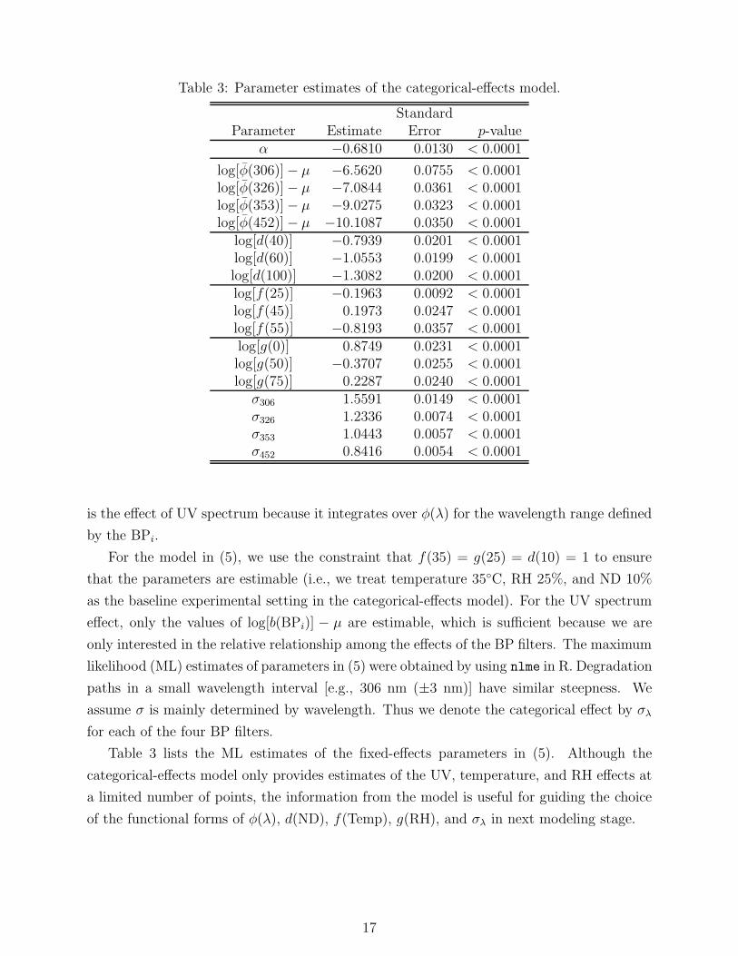
Table 3: Parameter estimates of the categorical-effects model.

StandardParameter Estimate Error p-value

α −0.6810 0.0130 < 0.0001

log[φ(306)]− µ −6.5620 0.0755 < 0.0001log[φ(326)]− µ −7.0844 0.0361 < 0.0001log[φ(353)]− µ −9.0275 0.0323 < 0.0001log[φ(452)]− µ −10.1087 0.0350 < 0.0001

log[d(40)] −0.7939 0.0201 < 0.0001log[d(60)] −1.0553 0.0199 < 0.0001log[d(100)] −1.3082 0.0200 < 0.0001log[f(25)] −0.1963 0.0092 < 0.0001log[f(45)] 0.1973 0.0247 < 0.0001log[f(55)] −0.8193 0.0357 < 0.0001log[g(0)] 0.8749 0.0231 < 0.0001log[g(50)] −0.3707 0.0255 < 0.0001log[g(75)] 0.2287 0.0240 < 0.0001

σ306 1.5591 0.0149 < 0.0001σ326 1.2336 0.0074 < 0.0001σ353 1.0443 0.0057 < 0.0001σ452 0.8416 0.0054 < 0.0001

is the effect of UV spectrum because it integrates over φ(λ) for the wavelength range defined

by the BPi.

For the model in (5), we use the constraint that f(35) = g(25) = d(10) = 1 to ensure

that the parameters are estimable (i.e., we treat temperature 35◦C, RH 25%, and ND 10%

as the baseline experimental setting in the categorical-effects model). For the UV spectrum

effect, only the values of log[b(BPi)] − µ are estimable, which is sufficient because we are

only interested in the relative relationship among the effects of the BP filters. The maximum

likelihood (ML) estimates of parameters in (5) were obtained by using nlme in R. Degradation

paths in a small wavelength interval [e.g., 306 nm (±3 nm)] have similar steepness. We

assume σ is mainly determined by wavelength. Thus we denote the categorical effect by σλ

for each of the four BP filters.

Table 3 lists the ML estimates of the fixed-effects parameters in (5). Although the

categorical-effects model only provides estimates of the UV, temperature, and RH effects at

a limited number of points, the information from the model is useful for guiding the choice

of the functional forms of φ(λ), d(ND), f(Temp), g(RH), and σλ in next modeling stage.

17

300 350 400 450 500

−11

−10

−9

−8

−7

−6

BP Filter Effect

Wavelength (nm)

0 20 40 60 80 100

−1.5

−1.0

−0.5

0.0

ND Filter Effect

Neutral Density (%)

20 30 40 50 60

−1.0

−0.8

−0.6

−0.4

−0.2

0.0

0.2

Temperature Effect

Temperature (Degree)

0 20 40 60 80 100

−0.5

0.0

0.5

1.0

RH Effect

RH (%)

Figure 7: Plots of the categorical effects for UV spectrum, ND filter, temperature, and RH.

4.2 Effects of the Explanatory Variables

In this section, we discuss the selection of the functional forms for the effects of explanatory

variables used in the laboratory accelerated test.

4.2.1 Modeling the BP Filter Effect

To suggest a functional form for φ(λ), we initially assume that φ(λ) is constant over the

specific range of each BP filter, denoted by φ(λ). For example, for the 306 nm BP filter,

φ(306) will be used to represent the effect. From (6), we obtain b(BPi) = [Di(ti)/ti]φ(λ).

Because we record Di(ti) and have an estimate of b(BPi) from the categorical-effects model,

we can obtain a heuristic estimate for φ(λ) from this relationship. For example,

φ(306) =b(306)

(∑

i:BPi=306[Di(ti)/ti])/(∑

i:BPi=306 1), (7)

for 303 nm ≤ λ ≤ 309 nm. Similarly, one can obtain the estimates of φ(λ) for other the BP

filters, 320 nm ≤ λ ≤ 332 nm, 332 nm ≤ λ ≤ 374 nm, and 373 nm ≤ λ ≤ 531 nm. The

corresponding results are shown in Table 3. Figure 7(a) provides a visualization of a simple

estimate of φ(λ). The results suggest that for shorter wavelengths, there is more damage

than at longer wavelengths, agreeing with known theory. The shape of the curve suggests

an exponential relationship.

The quasi-quantum yield φ(λ) describes the fact that photons at shorter wavelengths have

higher energy and thus a higher probability of causing damage. Martin, Lechner, and Varner (1994)

18

say that for polymeric materials, the shape of φ(λ) is typically exponential decay. The em-

pirical results in our categorical-effects model also suggest this and thus we use a log-linear

function φ(λ) = exp(β0+βλλ), to describe quasi-quantum yield where β0 and βλ are param-

eters to be estimated from the data.

The parameter σ in (5) is related to the slope of the degradation path. Because UV

is the main cause of degradation and shorter wavelength paths tend to have larger slopes,

we model σ as a function of λ. The curve of categorical-effects estimates of σλ versus λ

suggests an exponential relationship with a lower bound. Thus we use the functional form

σλ = σ0 + exp(σ1 + σ2λ) to describe the effect that UV wavelength has on σ.

From (5), one needs to have a wavelength specific dosage Dit(λ) to estimate the param-

eters in φ(λ) (i.e., β0 and βλ). For the laboratory accelerated test data, however, only the

aggregated dosage Di(t) data was available. We use an approximate method to obtain Dit(λ)

from Di(t). We consider the four intervals 303 nm ≤ λ ≤ 309 nm, 320 nm ≤ λ ≤ 332 nm,

332 nm ≤ λ ≤ 374 nm, and 373 nm ≤ λ ≤ 531 nm, corresponding to the four BP fil-

ters. Note that the spectral irradiance after filtering is Lamp(λ)Filter(λ,BPi,NDi), and the

approximate trapezoid area under each λ interval is denoted as Areaλ. The integration of

Areaλ over each of the four wavelength interval is denoted by Areaλ, where λ is 306 nm,

326 nm, 353 nm or 452nm, the BP filter nominal center points. We define the proportion of

area under λ relative to its corresponding wavelength range as P (λ) = Areaλ/Areaλ. Note

that

Di(t) =

∫ t

0

∫

λ

Lamp(λ)Filter(λ,BPi,NDi){1− exp[−A(λ)]}dλdτ, (8)

and the specific form of A(λ) is unknown. For the narrow intervals 303 nm ≤ λ ≤ 309 nm and

320 nm ≤ λ ≤ 332 nm, we can assume {1− exp[−A(λ)]} is constant because the fluctuation

over the narrow range of wavelengths is relatively small. Thus, for 303 nm ≤ λ ≤ 309 nm and

320 nm ≤ λ ≤ 332 nm, we obtain approximate values from Dit(λ) = Di(t)P (λ). Although

the interval 373 nm ≤ λ ≤ 531 nm is wide, the variation in Dit(λ) will be small because

both {1 − exp[−A(λ)]} and φ(λ) are small over the interval. Thus we can assume that

Dit(λ) is constant for 373 nm ≤ λ ≤ 531 nm. For the 332 nm ≤ λ ≤ 374 nm, the lamp

spectra curve is complicated and {1 − exp[−A(λ)]} is typically not small enough to do a

trapezoid approximation. Thus, in the subsequent modeling, we (as in the categorical-effects

model) use φ(353) to represent the effect of the 353 nm BP filter and treat it as an unknown

parameter to be estimated from the data. There is, however, enough information from the

other three BP filters for us to estimate the unknown parameters of the log-linear relationship

for φ(λ).

19

4.2.2 ND Filter Effect

A power law relationship is typically used to describe the ND effect (e.g., James 1997).

The power law relationship is based on Schwarzschild’s law, which says that the photo-

response of radiation over a given time period has a form NDp, where ND is the UV intensity

level. To achieve the same photo-response, NDp × t should be the same, where p is the

Schwarzschild coefficient and t is the exposure time. When p = 1, this relationship is called

the reciprocity law. Experimental deviations from the reciprocity law are called reciprocity

law failure. More discussion about Schwarzschild’s law and reciprocity can be found in

Martin, Chin, and Nguyen (2003).

Figure 7(b) shows the effects of the ND filter. A power law relationship d(NDi) = NDip

gives a perfect fit to the four points. Note that the Filter(λ,BPi,NDi) already includes the

effect of the ND filter as NDi with a power of one. Thus, the overall effect of ND filter is

NDi(1+p). If the reciprocity law (i.e., the effect of ND is NDi

1) holds, p should be equal to

zero in this parameterization. Thus, combining the physical knowledge and the empirical

evidence, we used the power law relationship to describe the UV intensity effects. Another

way of thinking about this is that with the reparameterization, the effect p describes the

deviation between nominal properties of the ND filters and the actual amount of photon

attenuation provided by the ND filters.

4.2.3 Temperature Effect

Figure 7(c) shows the effect that temperature has on the degradation rate. The Arrhenius

relationship is widely used to describe the acceleration effect of temperature on the rate of

a chemical reaction (e.g., Meeker, Escobar, and Lu 1998). According to the Arrhenius rela-

tionship, the logarithm of the reaction rate should be proportional to reciprocal temperature

in the Kelvin scale. In particular, the Arrhenius relationship is

f(Tempi) = γ0 exp

(−Ea/R

TempKi

), (9)

where TempKi is the Kelvin temperature computed as Celsius temperature plus 273.15,

Ea is the effective activation energy, and R is a gas constant. We define Ea/R to be the

temperature effect to be estimated from the data. The categorical-effects estimates agree

well with this relationship except for the specimens at 55◦C and 75 %RH.

A possible explanation for the change in the estimated temperature effect at 55◦C is

that there is an interaction between the high temperature and the high RH level. Such an

interaction could arise because water release is known to affect the rate of degradation. We

can not, however, estimate the interaction effect because there is data at 55◦C for only one

RH level. Another possible explanation is that there had been a failure of an integrated

circuit chip in a controller that caused certain chambers to be overheated for a period of

20

time. This could have lead to a different failure mechanism for the affected specimens. Based

on these considerations, we still use the Arrhenius relationship to model the temperature

effect after removing the data at 55◦C and 75% RH.

4.2.4 RH Effect

The effect of relative humidity on coating degradation is complicated. There are few theo-

retical results to suggest the functional form for humidity effect in this type of application.

It is known that low humidity will accelerate the side-chain scission process. As more end

groups are created, the degradation rate will tend to increase. On the other hand, higher

water content in the coating (caused by higher levels of RH) will tend to increase the diffu-

sion rate of oxygen in the oxidation zone, which can also increase the degradation rate (e.g.,

Chen and Fuller 2009, and Kiil 2009). Thus, there is a middle range of RH values where the

degradation rate would be expected to be smaller than at the extremes. These mechanisms

suggest a hump shape function for the effect that RH has on degradation. Figure 7(d) shows

the categorical-effects model estimates for the RH effect. The effect is increasing first and

then decreasing, suggesting a concave relationship. Based on the empirical evidence and the

suspected chemical reaction mechanisms, we used a quadratic model

log[g(RH)] = −βRH(RH− rh0)2 (10)

to describe the RH effect. Here, βRH and rh0 are unknown parameters to be estimated from

the data.

4.3 The Combined Model

Combining all of the identified functional forms for the effects of the experimental variables

gives following model for the underlying degradation path,

Gi(tij) =αexp(vi)

1 + exp(−z), (11)

where

z =η0 + log[Di(tij)] + A+ p(log[NDi])−

(Ea/R

TempKi

)− βRH (RHi − rh0)

2

σ0 + exp(σ1 + σ2λ),

A = log

[∫ λmax

λmin

P (λ) exp(βλλ)dλ

],

and vi is the random effect. Note that the total effective dosage for wavelength λ is Si(t, λ) =

Dit(λ) exp(β0 + βλλ), which is proportional to Dit(λ) exp(βλλ). We use Di(t) × P (λ) ×

exp(βλλ) to approximate Dit(λ) exp(βλλ). We define the constant η0 = β0 + log(γ0) − µ

21

Table 4: Parameter estimates for the combined model in (11).

StandardParameter Estimate Error p-value

α −0.6191 0.01013 < 0.0001βλ −0.0297 0.00026 < 0.0001p −0.5606 0.00781 < 0.0001Ea

R1945.6482 75.83458 < 0.0001

βRH −0.0005 0.00001 < 0.0001rh0 45.4748 0.28749 < 0.0001η0 9.8986 0.25662 < 0.0001

b(353) −11.5661 0.09428 < 0.0001σ0 0.8019 0.00664 < 0.0001σ1 7.6776 0.18760 < 0.0001σ2 −0.0260 0.00062 < 0.0001

because the µ and the individual intercept terms are not independently estimable in the

model.

Table 4 lists the ML estimates of the parameters in (11). The maximum degradation

damage when total effective dosage goes to infinity is −0.6191, not considering random ef-

fects. For the ND filter effect, the power p is estimated to be −0.5606, which is significantly

different from 0. Thus there is evidence that the reciprocity law does not hold in this ap-

plication. The combined ND effect in Filter(λ,BPi,NDi) is 1 − 0.5606 = 0.4394. That is,

ND0.4394 describes the overall effect of the ND filters. For example, the effect of a nomi-

nal 80% ND filter is 100(0.800.4394)% = 90.6% filtering. As expected, the quasi-quantum

yield coefficient βλ = −0.0297 < 0 indicating that shorter wavelengths cause more damage.

Figure 8 shows examples of our model (11) fitted to the laboratory accelerated test data,

showing good agreement.

5 The Prediction Model for Outdoor-Exposure Data

In this section, we adapt the laboratory accelerated test model (11) and its parameter esti-

mates to predict outdoor-exposure degradation.

5.1 The Cumulative Damage Model for Outdoor-Exposure Degra-

dation Prediction

For computational convenience, we used 60 minutes instead of 12 minutes as the time interval

for the dynamic covariates. For outdoor-exposure specimen k, we define the incremental

22

0 200 400 600

−0.6

−0.5

−0.4

−0.3

−0.2

−0.1

0.0

BP: 326nm, ND: 10%, T: 35C, RH: 0%

DosageD

amag

e A

mou

nts

0 500 1000 1500

−0.6

−0.5

−0.4

−0.3

−0.2

−0.1

0.0

BP: 306nm, ND: 100%, T: 25C, RH: 0%

Dosage

Dam

age

Am

ount

s0 1000 2000 3000

−0.6

−0.5

−0.4

−0.3

−0.2

−0.1

0.0

BP: 326nm, ND: 40%, T: 45C, RH: 75%

Dosage

Dam

age

Am

ount

s

0 20000 40000 60000

−0.6

−0.5

−0.4

−0.3

−0.2

−0.1

0.0

BP: 353nm, ND: 40%, T: 35C, RH: 0%

DosageD

amag

e A

mou

nts

Figure 8: Fitted degradation paths for four randomly selected specimens based on the model

in (11). The points are the measured values and the lines show the fitted values. The plot

titles show the levels of the experimental factors.

effective dosage at wavelength interval λ± 1 over the 60-minute interval starting at τ to be

∆S∗

k(τ, λ) =

∫ τ+60 min

τ

∫ λ+1nm

λ−1 nm

Dk(τ, λ) exp(βλλ)dλdτ. (12)

Here we use an “∗” to indicate that the difference from the effective dosage defined previously.

The previous definition used φ(λ) but here we use exp(βλλ), which is proportional to φ(λ).

The effective dosage across all wavelengths at time τ is S∗

kτ (τ) =∫λ∆S∗

k(τ, λ)dλ. The

cumulative total effective dosage across all wavelengths from time 0 to time t is S∗

k(t) =∫ t

0S∗

kτ(τ)dτ . Temperature and RH are averaged over all 60-minute intervals. Because no

ND filters were used during the outdoor exposures, we set ND to be 100% for all outdoor-

exposure predictions.

According to the cumulative damage model, the slope of the degradation curve at time

τ and wavelength λ is a function of total effective dosage S∗

k(τ) and other environmental

effects. That is,

g′k(τ, λ) =dGk(τ)

d[S∗

k(τ)]=

1

S∗

k(τ)σλ×

α exp(z)

[1 + exp(z)]2, (13)

where

z =log[S∗

k(τ)] + η0 + p[log(ND)]−[

Ea/RTemp

k(τ)+273.15

]− βRH [RHk(τ)− rh0]

2

σ0 + exp (σ1 + σ2λ). (14)

23

Note that here we compute the slope g′k(τ, λ) as a function of τ and λ because σλ depends

on λ and the incremental damage amounts need to be accumulated across the time τ and

wavelength λ intervals. The incremental damage, ∆Gk(τ, λ), is the damage at time τ that

was caused by the UV radiation in the 2nm wavelength interval (λ− 1, λ+1). In particular,

∆Gk(τ, λ) = g′k(τ, λ)∆S∗

k(τ, λ). The additivity law is assumed, implying that the damage can

be summed up from each wavelength interval in every 60-minute time interval. Then ∆Gk(τ)

denotes incremental damage at time τ from all wavelengths, ∆Gk(τ) =∑

λ ∆Gk(τ, λ). The

cumulative damage Gk(t) from time 0 to t from all wavelengths is

Gk(t) =t∑

τ=0

∆Gk(τ). (15)

Hence, degradation Gk(t) can be predicted based on the model estimated from the laboratory

accelerated test data. Because there is a random effect vk in the mean structure Gk(t), for

the point prediction, we set vk to be zero when computing point predictions.

5.2 Outdoor-Exposure Prediction Uncertainty Quantification

The outdoor-exposure prediction involves two sources of variability: the random effect vk

and the variability in θ. Here we use θ to denote all the parameters in (11), and θ

is the ML estimator. The corresponding variance-covariance matrix is denoted by Σθ.

We use prediction intervals to quantify the prediction uncertainty. Prediction intervals

are calculated and calibrated following a procedure that is similar to those described in

Hong, Meeker, and McCalley (2009), using the Lawless and Fredette (2005) predictive dis-

tribution. For notational simplicity, let G = Gk(t), because we compute pointwise prediction

intervals. The cumulative distribution function of G at a particular point in time t is de-

noted by F (G; θ) which is primarily determined by the distribution of the random effect. In

particular, the algorithm to compute the predictive distribution is,

1. Simulate B sample estimates θ∗

b ∼ N(θ,Σθ) and v∗b ∼ N(0, σ2

v), b = 1, . . . , B. We use

B = 50,000.

2. Compute the degradation G∗

b , b = 1, . . . , B using the method summarized by (15) under

parameter θ∗

b and the random effect v∗b .

3. Compute W ∗

b = F (G∗

b |θ∗

b), b = 1, . . . , B.

4. Compute wl and wu, the lower and upper α/2 sample quantiles, respectively, of W ∗

b .

5. Solve F (Gl|θ) = wl, F (Gu|θ) = wu for (Gl,Gu), providing the 100(1 − α)% calibrated

prediction interval.

This algorithm needs to be repeated over the range of t values of interest.

24

5.3 Outdoor-Exposure Prediction Results and Model Compar-

isons

5.3.1 Outdoor-Exposure Predictions

Figure 9 compares the measured and predicted degradation paths based on our cumulative

damage model for the same representative set of outdoor-exposed sample paths shown in

Figure 5. The predicted values for some specimens agree well with the measured values, while

for others the predicted values are either above or below that of the actual outdoor-exposed

sample paths. These variations correspond to the distribution of the random effects. Most

of the measured data points are within the calibrated prediction intervals, except for some

small levels of degradation at early times which may have been caused by measurement

error. Because the random effects are modeled as normally distributed with mean 0, the

average predicted values should be close to the averaged measured values for all 53 outdoor-

exposed specimens. Figure 10 shows the average of predicted and measured damage for all

of the outdoor-exposed specimens. The average predicted values correspond well to average

measured values.

We saw that the random effects tend to be similar within the same outdoor-exposed group.

For example, four specimens from outdoor-exposed group G1 all have predictions larger than

the measured values. The four specimens from group G16OUT all have predictions smaller

than the measured values, and the four specimens from group G4 all have predictions close

to the measured values. These suggest that the random effects could be related to group

conditions such as additional weather-related effects not accounted for in our model. Other

factors that may contribute to the random effects include the non-uniform spatial irradiance

of specimens, possible non-uniformity of the material of the specimens, etc.

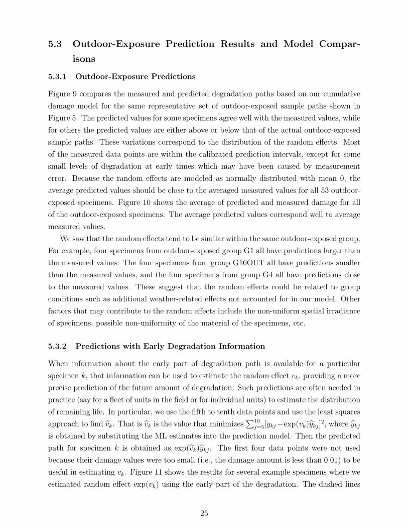
5.3.2 Predictions with Early Degradation Information

When information about the early part of degradation path is available for a particular

specimen k, that information can be used to estimate the random effect vk, providing a more

precise prediction of the future amount of degradation. Such predictions are often needed in

practice (say for a fleet of units in the field or for individual units) to estimate the distribution

of remaining life. In particular, we use the fifth to tenth data points and use the least squares

approach to find vk. That is vk is the value that minimizes∑10

j=5[ykj−exp(vk)ykj]2, where ykj

is obtained by substituting the ML estimates into the prediction model. Then the predicted

path for specimen k is obtained as exp(vk)ykj. The first four data points were not used

because their damage values were too small (i.e., the damage amount is less than 0.01) to be

useful in estimating vk. Figure 11 shows the results for several example specimens where we

estimated random effect exp(vk) using the early part of the degradation. The dashed lines

25

0 20 60

−0.6−0.5−0.4−0.3−0.2−0.1

0.0G11−10

0 20 40

−0.6−0.5−0.4−0.3−0.2−0.1

0.0G12−9

0 10 30 50

−0.6−0.5−0.4−0.3−0.2−0.1

0.0G16−11

0 10 30 50

−0.6−0.5−0.4−0.3−0.2−0.1

0.0G17−9

0 10 20 30

−0.6−0.5−0.4−0.3−0.2−0.1

0.0G16OUT−11

0 40 80 120

−0.6−0.5−0.4−0.3−0.2−0.1

0.0G1−8

0 50 100

−0.6−0.5−0.4−0.3−0.2−0.1

0.0G3−10

0 50 100 200

−0.6−0.5−0.4−0.3−0.2−0.1

0.0G4−11

0 20 60 100

−0.6−0.5−0.4−0.3−0.2−0.1

0.0G9−8

0 20 40 60

−0.6−0.5−0.4−0.3−0.2−0.1

0.0G11OUT−8

0 20 40 60 80

−0.6−0.5−0.4−0.3−0.2−0.1

0.0G15−8

0 50 100 150

−0.6−0.5−0.4−0.3−0.2−0.1

0.0G18−8

Days Since the First Measurement

Deg

rada

tion

Am

ount

s

Figure 9: Prediction results for 12 representative outdoor-exposed specimens. The points

show the measured values, the solid lines show the predicted values, and the dashed lines

show the 95% pointwise prediction intervals.

indicate the predicted values after adjusting. For most specimens, the adjusted predicted

values match the measured values considerably better than the unadjusted values.

5.3.3 Comparisons

This section describes comparisons among several models. We use the Akaike information

criterion (AIC) for model-fitting comparisons and mean squared error (MSE) for prediction

comparisons. We considered the following models for comparisons.

• Model A: A model similar to that used in Vaca-Trigo and Meeker (2009), using no

random effect and where UV intensity was not modeled directly.

• Model B: The model in (4) with individual random effects for each specimen and

carefully modeled effects for all of the experimental variables. For predictions from

this model, there are two variants.

– Model B1: Prediction with all random effects set equal to the expected value of

zero.

26

0 20 40 60 80

−0.35

−0.30

−0.25

−0.20

−0.15

−0.10

−0.05

Days Since the First Measurement

Dam

age

Am

ount

s

MeasuredPredicted

Figure 10: Plots of averaged outdoor-exposed degradation measurements and values pre-

dicted by the cumulative damage model.

0 20 60

−0.6−0.5−0.4−0.3−0.2−0.1

0.0G11−10

0 20 40

−0.6−0.5−0.4−0.3−0.2−0.1

0.0G12−9

0 10 30 50

−0.6−0.5−0.4−0.3−0.2−0.1

0.0G16−11

0 10 30 50

−0.6−0.5−0.4−0.3−0.2−0.1

0.0G17−9

0 10 20 30

−0.6−0.5−0.4−0.3−0.2−0.1

0.0G16OUT−11

0 40 80 120

−0.6−0.5−0.4−0.3−0.2−0.1

0.0G1−8

0 50 100

−0.6−0.5−0.4−0.3−0.2−0.1

0.0G3−10

0 50 100 200

−0.6−0.5−0.4−0.3−0.2−0.1

0.0G4−11

0 20 60 100

−0.6−0.5−0.4−0.3−0.2−0.1

0.0G9−8

0 20 40 60

−0.6−0.5−0.4−0.3−0.2−0.1

0.0G11OUT−8

0 20 40 60 80

−0.6−0.5−0.4−0.3−0.2−0.1

0.0G15−8

0 50 100 150

−0.6−0.5−0.4−0.3−0.2−0.1

0.0G18−8

Days Since the First Measurement

Deg

rada

tion

Am

ount

s

Figure 11: Prediction results for 12 representative outdoor-exposed specimens, with ad-

justment made by random effects estimated from the 5th to 10th data points. The points

show the measured values, the solid lines show the predictions without adjustments, and the

dashed lines show the predictions with adjustments.

27

Table 5: Comparisons of model fits and predictions.

ModelLog likelihood Number of

AICPrediction

values parameters Model MSEA 15740.22 9 −31462.44 A 0.004238

B 30201.98 13 −60377.95B1 0.002879B2 0.002522

C 30414.43 14 −60800.85C1 0.002524C2 0.002396

– Model B2: Prediction using some of the early data points to estimate the random

effects for the individual specimens.

• Model C: The model in (4) can be easily extended to more complicated random-effects

structures. For Model C, we consider the model in (4) but with both specimen-to-

specimen and group-to-group random effects. Note that there were typically four

replicates within experimental group (i.e., exposed at the same time and in the same

chamber). For predictions from this model, we also have two variants.

– Model C1: Prediction with all random effects set equal to the expected value of

zero.

– Model C2: Prediction using some of the early data points to estimate the random

effects for the groups and the individual specimens.

Table 5 shows the model comparison results. The results show that the proposed Models B

and C provide a much better fit to the laboratory accelerated test data than the model in

Vaca-Trigo and Meeker (2009). There is not much difference between the prediction perfor-

mance of Models B and C. Both models provide much better predictions than Model A.

6 Conclusions and Areas for Future Research

This paper describes the development of an accelerated test methodology for photodegra-

dation, including a predictive model that uses laboratory accelerated degradation test data

to predict the service life of specimens subjected to outdoor exposure. The methodology

was verified by predicting damage for similar specimens that were exposed outdoors. We

developed a physically motivated nonlinear regression model with random effects to describe

the laboratory accelerated test degradation data, carefully studied the functional forms of

the experimental variables to develop the model, and estimated model parameters from the

accelerated test data. Then we used a cumulative damage model, incorporating the pa-

rameter estimates from the laboratory accelerated test and individual specimen dynamic

28

covariate information, to predict the individual outdoor-exposed degradation paths. We also

developed an algorithm to calculate the prediction intervals. In addition, we showed how

to estimate the specimen-to-specimen random effect for an individual specimen, providing a

means of predicting remaining service life for a unit that has been in service.

The degradation modeling and prediction methods presented in this paper serve as an

important step in the development of the science of outdoor weathering service life prediction.

There are, however, several areas for further research.

• Given a probability model for degradation paths (such as the one developed in this pa-

per) and corresponding random effects, a specific set of dynamic-covariate time series,

and a definition of the corresponding soft-failure threshold, it is possible to compute the

failure-time distribution for exposed units. Chapter 13 of Meeker and Escobar (1998)

illustrates this for simple constant-environment situations. The ideas there could

be generalized to compute an estimate of a failure-time distribution for a specified

dynamic-covariate history. In general, evaluation will require simulation.

• A further extension could use a model for the dynamic covariates (similar to that used in

Hong et al. 2015) to find a failure-time distribution that takes into account uncertainty

in the future realizations of the dynamic covariates. Models with autocorrelation for

the error terms in (3) can also be considered.

• The predictions generated in this paper and the corresponding failure-time distribu-

tions mentioned above correspond to a given “weather” realization from the model

for the weather which might be a “typical” realization or, perhaps, a harsher one, to

get more conservative predictions. If there were a need to predict actual failures for a

population of product units in the field, then one would have to consider a mixture of

different weather models and generate predictions for each, weighted by the amount of

product subject to each such weather model.

• In general, outdoor environments are complicated. In the NIST outdoor-exposure ex-

periments, the specimens were placed in a covered chamber so that the main driving

factors were UV, temperature, and RH. A more extensive experiment could be con-

ducted to study the effect of factors like contaminants in the air, dust, acid rain, and

extreme events.

Acknowledgments

The authors thank the editor, an associate editor, and the referees, for their valuable com-

ments that lead to significant improvement on this paper. The authors acknowledge Ad-

vanced Research Computing at Virginia Tech for providing computational resources. The

29

work by Hong was partially supported by the National Science Foundation under Grant

CMMI-1634867 to Virginia Tech.

References

Bagdonavicius, V. and M. S. Nikulin (2001). Estimation in degradation models with ex-

planatory variables. Lifetime Data Analysis 7, 85–103.

Bellinger, V. and J. Verdu (1984). Structure-photooxidative stability relationship of amine-

crosslinked epoxies. Polymer Photochem 5, 295–311.

Bellinger, V. and J. Verdu (1985). Oxidative skeleton breaking in Epoxy-Amine networks.

Journal of Applied Polymer Science 30, 363–374.

Chen, C. and T. F. Fuller (2009). The effect of humidity on the degradation of Nafion

membrane. Polymer Degradation and Stability 94, 1436–1447.

Cox, D. R. and D. Oakes (1984). Analysis of Survival Data, Volume 21. Boca Raton, FL:

CRC Press.

Davidian, M. and D. M. Giltinan (2003). Nonlinear models for repeated measurement

data: An overview and update. Journal of Agricultural, Biological, and Environmental

Statistics 8, 387–419.

Escobar, L. A. and W. Q. Meeker (2006). A review of accelerated test models. Statistical

Science 21, 552–577.

Gu, X., B. Dickens, D. Stanley, W. Byrd, T. Nguyen, I. Vaca-Trigo, W. Q. Meeker, J. Chin,

and J. Martin (2009). Linking accelerating laboratory test with outdoor performance

results for a model epoxy coating system. In J. W. Martin, R. A. Ryntz, J. Chin, and

R. A. Dickie (Eds.), Service Life Prediction of Polymeric Materials, Global Perspec-

tives, pp. 3–28. NY: New York: Springer.

Hahn, G. J. and N. Doganaksoy (2008). The Role of Statistics in Business and Industry.

Hoboken, New Jersey: John Wiley & Sons, Inc.

Hong, Y., Y. Duan, W. Q. Meeker, X. Gu, and D. Stanley (2015). Statistical methods for

degradation data with dynamic covariates information and an application to outdoor

weathering data. Technometrics 57, 180–193.

Hong, Y. and W. Q. Meeker (2010). Field-failure and warranty prediction based on aux-

iliary use-rate information. Technometrics 52, 148–159.

Hong, Y. and W. Q. Meeker (2011). A model for field-failure prediction using dynamic en-

vironmental data. In N. Balakrishnan, M. Nikulin, and V. Rykov (Eds.), Mathematical

30

and Statistical Methods in Reliability. Applications to Medicine, Finance and Quality

Control, Chapter 16, pp. 223–233. Birkhauser: Boston.

Hong, Y., W. Q. Meeker, and J. D. McCalley (2009). Prediction of remaining life of power

transformers based on left truncated and right censored lifetime data. The Annals of

Applied Statistics 3, 857–879.

James, T. (1997). The Theory of the Photographic Process (fourth ed.). New York: Macmil-

lan.

Kelleher, P. and B. Gesner (1969). Photo-oxidation of phenoxy resin. Journal of Applied

Polymer Science 13, 9–15.

Kiil, S. (2009). Model-based analysis of photoinitiated coating degradation under artificial

exposure conditions. Journal of Coatings Technology and Research 9, 375–398.

Lawless, J. F. and M. Fredette (2005). Frequentist prediction intervals and predictive

distributions. Biometrika 92, 529–542.

Lu, C. J. and W. Q. Meeker (1993). Using degradation measures to estimate a time-to-

failure distribution. Technometrics 34, 161–174.

Martin, J. W., J. W. Chin, and T. Nguyen (2003). Reciprocity law experiments in poly-

meric photodegradation: a critical review. Progress in Organic Coatings 47, 292–311.

Martin, J. W., J. A. Lechner, and R. N. Varner (1994). Quantitative characterization of

photodegradation effects of polymeric materials exposed in weathering environments.

In W. D. Ketola and D. Grossman (Eds.), Accelerated and Outdoor Durability Testing

of Organic Materials, ASTM-STP-1202. Philadelphia: American Society for Testing

and Materials.

Martin, J. W., S. C. Saunders, F. L. Floyd, and J. P. Wineburg (1996). Methodologies for

predicting the service lives of coating systems. In D. Brezinski and T. Miranda (Eds.),

Federation Series on Coating Technology, pp. 1–32. Blue Hill, PA: Federation Series

on Coating Technology.

Meeker, W. Q. and L. A. Escobar (1998). Statistical Methods for Reliability Data. New

York: John Wiley & Sons, Inc.

Meeker, W. Q., L. A. Escobar, and C. J. Lu (1998). Accelerated degradation tests: mod-

eling and analysis. Technometrics 40, 89–99.

Meeker, W. Q., Y. Hong, and L. A. Escobar (2011). Degradation models and data analyses.

In Encyclopedia of Statistical Sciences, pp. 1–23. Hoboken, NJ: John Wiley & Sons,

Inc.

Nelson, W. (1990). Accelerated Testing: Statistical Models, Test Plans, and Data Analyses.

New York: John Wiley & Sons.

31

Pinheiro, J. and D. Bates (2006). Mixed-effects models in S and S-PLUS. NY: New York:

Springer Science & Business Media.

Rabek, J. (1995). Polymer Photodegradation-Mechanisms and Experimental Methods. Lon-

don, UK: Chapman & Hall.

Spurgeon, K., W. H. Tang, Q. H. Wu, Z. J. Richardson, and G. Moss (2005). Dissolved

gas analysis using evidential reasoning. IEEE Proceedings - Science, Measurement &

Technology 152, 110–117.

Subramanian, S., K. Reifsnider, and W. Stinchcomb (1995). A cumulative damage model

to predict the fatigue life of composite laminates including the effect of a fibre-matrix

interphase. International Journal of Fatigue 17, 343–351.

Vaca-Trigo, I. and W. Q. Meeker (2009). A statistical model for linking field and laboratory

exposure results for a model coating. In J. Martin, R. A. Ryntz, J. Chin, and R. A.

Dickie (Eds.), Service Life Prediction of Polymeric Materials, pp. 29–43. New York,

NY: Springer.

Xu, Z., Y. Hong, and R. Jin (2016). Nonlinear general path models for degradation data

with dynamic covariates. Applied Stochastic Models in Business and Industry 32, 153–

167.

32