1

Development of Version 2 of the Wildland Fire Portion

of the National Emissions Inventory

Sean M. Raffuse

Sonoma Technology, Inc., 1455 N. McDowell Blvd., Suite D, Petaluma, CA 94954

sraffuse@sonomatech.com

Narasimhan K. Larkin and Peter W. Lahm

USDA Forest Service, 400 N. 34th Street, Suite 201, Seattle, WA 98103

Yuan Du

Sonoma Technology, Inc.

ABSTRACT

Emissions from wildland fires represent a large fraction of the total mass of particulate matter

emitted in the United States. We present the methods and results for the national-scale

processing of version 2 of the 2008 wildland fire National Emissions Inventory (NEI). The

version 2 NEI was produced using fire activity data from SmartFire 2 (SF2) and emissions

processing in the BlueSky smoke modeling framework. Additionally, guidance and feedback

from experts were utilized in determining input data sets and processing streams. This is

important because both BlueSky and the newly redesigned SF2 are frameworks that contain

multiple modeling processing pathways and options. Wildland fire emissions of PM2.5 were

estimated at 1,716,000 tons, which represents 28% of the total PM2.5 from the NEI.

INTRODUCTION

Wildland fires, including wildfires and prescribed burning, represent a significant fraction of the

total emissions of fine particles, both globally and nationally.1 Unfortunately, there is still

significant uncertainty in wildland fire emission estimates.2 In spite of this, the United States

Environmental Protection Agency (EPA) must produce an inventory for wildland fires every

three years as part of the National Emissions Inventory (NEI), which is used for regulatory

modeling and analysis. Therefore, it is important to continually improve methods to estimate

wildland fires in the U.S.

Emissions from wildland fire can be thought of in terms of the classic formula of Seiler and

Crutzen (1980):

(1)

where

= area burned

= biomass available (or fuel loading)

= combustion efficiency (or consumption)

= an emission factor for pollutant or group i

2

Equation 1 is commonly used in developing biomass burning emissions estimates; however, the

equation masks considerable complexity. The area burned term can be derived from remote

sensing of active fires, remote sensing of burn scars, ground-based reporting, or some

combination. These methods of estimating area burned do not necessarily yield similar results.

Biomass available for burning within the burned area (known as the fuel loading) can be of a

variety of different vegetation types and estimated from several different mappings and

methodologies. Combustion efficiency is a function of how much of the fuel loading is

consumed, which is estimated by consumption models that take into account the fuel types,

forest structure, and fuel loadings along with fuel moisture and type of fire. These complex

dynamic or empirical consumption models include Consume,3 and the First Order Fire Effects

Model.4

This paper presents methods and results for the 2008 national wildland fire emissions inventory

that serves as the basis for the wildland fire component of the 2008 NEI (version 2). Wildland

fire includes wildfires and prescribed burns, but does not include agricultural burning, which is

estimated separately. The final 2008 NEI version 2 published by the EPA differs from what is

presented here in that the NEI also contains data submitted by several states (sometimes in lieu

of the data presented here and sometimes in combination with the data presented here). Despite

this, wildland fire emissions estimates for most states in the final NEI come from this analysis.

Though the NEI includes estimates for several pollutants, we focus on PM2.5, the pollutant for

which wildland fires represent the largest fraction of the overall U.S. inventory.

METHODS

We present the overall methods used in the NEI (version 2) national scale processing below. For

additional details, please refer to the full General Technical Report, which can be found at

http://airfire.org/emissions.

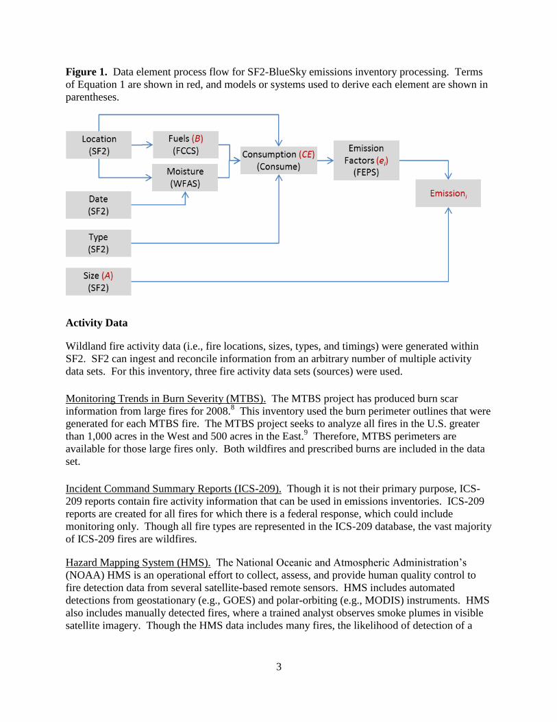
The flow of data elements used to produce the terms in Equation 1 is shown in Figure 1. Fire

activity information (location, date, type, and size of fires) is provided by SmartFire version 2.0

(SF2). Although SF2 shares some features with the original SmartFire system, SF2 has been

comprehensively redesigned to be more flexible, expandable, and accurate. SF2 is a modular

framework that can combine an indefinite number of fire information data sets (ground reports,

satellite-based detection, helicopter perimeters, etc.) into a best estimate of fire activity.

The remaining elements are calculated using models or data sets within the BlueSky framework,5

including LANDFIRE-mapped fuelbeds from the Fuel Characteristic Classification System,6

Consume, and the Fire Emissions Production Simulator,7 and fuel moisture calculations from the

Wildland Fire Assessment System (WFAS) archive. Each processing step is outlined below.

3

Figure 1. Data element process flow for SF2-BlueSky emissions inventory processing. Terms

of Equation 1 are shown in red, and models or systems used to derive each element are shown in

parentheses.

Activity Data

Wildland fire activity data (i.e., fire locations, sizes, types, and timings) were generated within

SF2. SF2 can ingest and reconcile information from an arbitrary number of multiple activity

data sets. For this inventory, three fire activity data sets (sources) were used.

Monitoring Trends in Burn Severity (MTBS). The MTBS project has produced burn scar

information from large fires for 2008.8 This inventory used the burn perimeter outlines that were

generated for each MTBS fire. The MTBS project seeks to analyze all fires in the U.S. greater

than 1,000 acres in the West and 500 acres in the East.9 Therefore, MTBS perimeters are

available for those large fires only. Both wildfires and prescribed burns are included in the data

set.

Incident Command Summary Reports (ICS-209). Though it is not their primary purpose, ICS-

209 reports contain fire activity information that can be used in emissions inventories. ICS-209

reports are created for all fires for which there is a federal response, which could include

monitoring only. Though all fire types are represented in the ICS-209 database, the vast majority

of ICS-209 fires are wildfires.

Hazard Mapping System (HMS). The National Oceanic and Atmospheric Administration’s

(NOAA) HMS is an operational effort to collect, assess, and provide human quality control to

fire detection data from several satellite-based remote sensors. HMS includes automated

detections from geostationary (e.g., GOES) and polar-orbiting (e.g., MODIS) instruments. HMS

also includes manually detected fires, where a trained analyst observes smoke plumes in visible

satellite imagery. Though the HMS data includes many fires, the likelihood of detection of a

4

specific fire depends on many parameters, including size, intensity, land type, timing, and cloud

cover.

Association and Reconciliation

SF2 works by first associating data between input data sources that are likely to represent the

same actual real-world fire. SF2 then reconciles the associated data into a single coherent

information stream using a variety of options and user-adjustable weightings. The association

and reconciliation steps are done to (1) avoid double counting fires that appear in multiple data

sources and (2) allow for utilizing the best data sources for each piece of information required

(e.g., location, size, fire type).

In this inventory, data were associated using spatio-temporal overlap of the data with assumed

uncertainty bounds set for each data source, and associated data were reconciled using simple

precedence. For each key element, each data source was assigned a rank. For a given fire, the

data source with the highest rank in an element provided the estimate for that element. Table 1

shows the ranks that were assigned to each data source for each data element. We note that each

of the data sources included fires that were not present in any other data source.

Table 1. Data source precedence for the key data elements estimated by SF2.

Data Element First Choice Second Choice Third Choice

Location/shape MTBS HMS ICS-209

Final size MTBS ICS-209 HMS

Daily growtha HMS ICS-209 MTBS

Fire type (WF/Rx) ICS-209 MTBS climatology b

Name ICS-209 MTBS unique ID assigned

c

Start date First reported

End date HMS ICS-209 MTBS

a results are scaled to final size so daily growth is relative

b a climatology of prescribed fire vs. wildfire seasonality was used where no other type information was available

(see below) c

for fires not in the ICS or MTBS datasets, a unique name was assigned based on their HMS satellite detects

Final Size from HMS

“Final size” represents the total burned area of the fire. For fires with other information for final

size, HMS satellite detects were aggregated into an estimate of final fire size. HMS hot spot

pixels do not provide information on area burned intrinsically, so final size must be inferred.

Final size was estimated by assigning an area burned per pixel (Ap) and multiplying by the

5

number of pixels in the fire. The value of Ap depends on the ecosystem because the same fire

size will result in heat release, smoldering length, and timing differences in different ecosystems

and therefore result in different satellite detection probabilities. To develop the area-per-pixel

relationships, MTBS burn perimeters for 2003-2008 were intersected with the FCCS 1-km

resolution map (http://www.fs.fed.us/pnw/fera/fccs/maps.shtml). Each FCCS fuelbed and each

MTBS perimeter was assigned to one of 12 broad vegetation classes. Linear area-per-pixel

relationships were developed for fires that were less than 10,000 acres and for all fires. Figure 2

shows how Ap varies spatially.

Figure 2. Mapped values of Ap used for the determination of final size from HMS data.

Fire Type from Climatology

Where no other information on fire type is available, a fire type climatology was developed to

designate fires as either wildfire or prescribed burn depending on the state and month of the burn

(Figure 3). Fires were presumed to be prescribed burns unless they fell within the “distinct

wildfire season” for the state. The fire season map was developed by analyzing the MTBS data

set for the years 1984-2006 to determine the typical wildfire season for each state and analyzing

the Forest Service Activity Tracking (FACTS) prescribed burn data set for one year (10/1/2009

to 9/30/2010) to estimate the prescribed burning season. For many states in the West, the

seasonal patterns of wild and prescribed fires were distinct and separable. In other states,

particularly in the southeastern United States, the seasons were not separable. For those states,

fires lacking other information are presumed to be prescribed burns. Fires only found in the

6

HMS data source were presumed to be prescribed burns by default because wildfires were more

likely to be represented in the other data sets as well.

Figure 3. Default wildfire assignment map. If a fire with no type information fell within the

states and months shown, it was designated as a wildfire. Otherwise, it was assumed to be a

prescribed burn.

Emissions Processing

The fire activity data produced by the SF2 processing described above provided inputs to

emissions modeling within BlueSky. SF2 was used to produce reconciled fire activity output in

the BlueSky standard file format. The following steps were applied:

1) Segregate agricultural fires (based on the USGS National Land Cover Dataset)

2) Assign fuel moistures (via the USFS Wildland Fire Assessment System)

3) Process emissions through BlueSky:

a) Fuel loading (LANDFIRE-FCCS 1-km database)

b) Consumption (Consume 4.0)

c) Emissions (FEPS emissions factors)

4) Post-process (duff consumption adjustment)

Duff consumption for prescribed fires was adjusted as a post-process step because of a known

issue in the current Consume 4.0 model where unrealistically large duff consumption can occur

in areas of large duff depths. Because this issue was flagged by regional experts working with

the National Wildfire Coordinating Group’s Smoke Committee, a post-processing limitation was

imposed on prescribed fire duff consumption of 20 tons/acre in the western U.S. and 5 tons/acre

in the eastern U.S. No limitations were imposed on wildfire duff consumption.

7

RESULTS

The total 2008 PM2.5 from wild and prescribed fires was estimated at about 1,716,000 tons.

Table 2 compares this total with the overall PM2.5 in the 2008 NEI. Together, wild and

prescribed fires comprise 28% of the total U.S. PM2.5 inventory, with wildfires contributing 16%

and prescribed burning contributing 12%.

Table 2. Total PM2.5 emissions in the 2008 NEI and this study.

Sector PM2.5 emissions (tons) Percent of Total

2008 NEI v2 (all sectors) 6,066,086 100

This study (wild and prescribed fire) 1,715,962 28

This study (wildfire) 994,292 16

This study (prescribed fire) 721,670 12

Area burned and PM2.5 results by state and fire type are presented in Figure 4. Large area burned

totals are present throughout the southeast, the southern plains, and in California. With the

exception of California, area burned state totals are dominated by prescribed burning.

Conversely, the emissions pattern is dominated by wildfires, particularly in California, which

had a record wildfire season, and North Carolina, where a single wildfire burned deep into the

organic ground layer and produced significant emissions.

8

Figure 4. State totals of area burned (top) and PM2.5 emitted (bottom) by fire type. Pie sizes are

proportional to state totals. Each pie consists of two components: prescribed fire (green) and

wildfire (red).

9

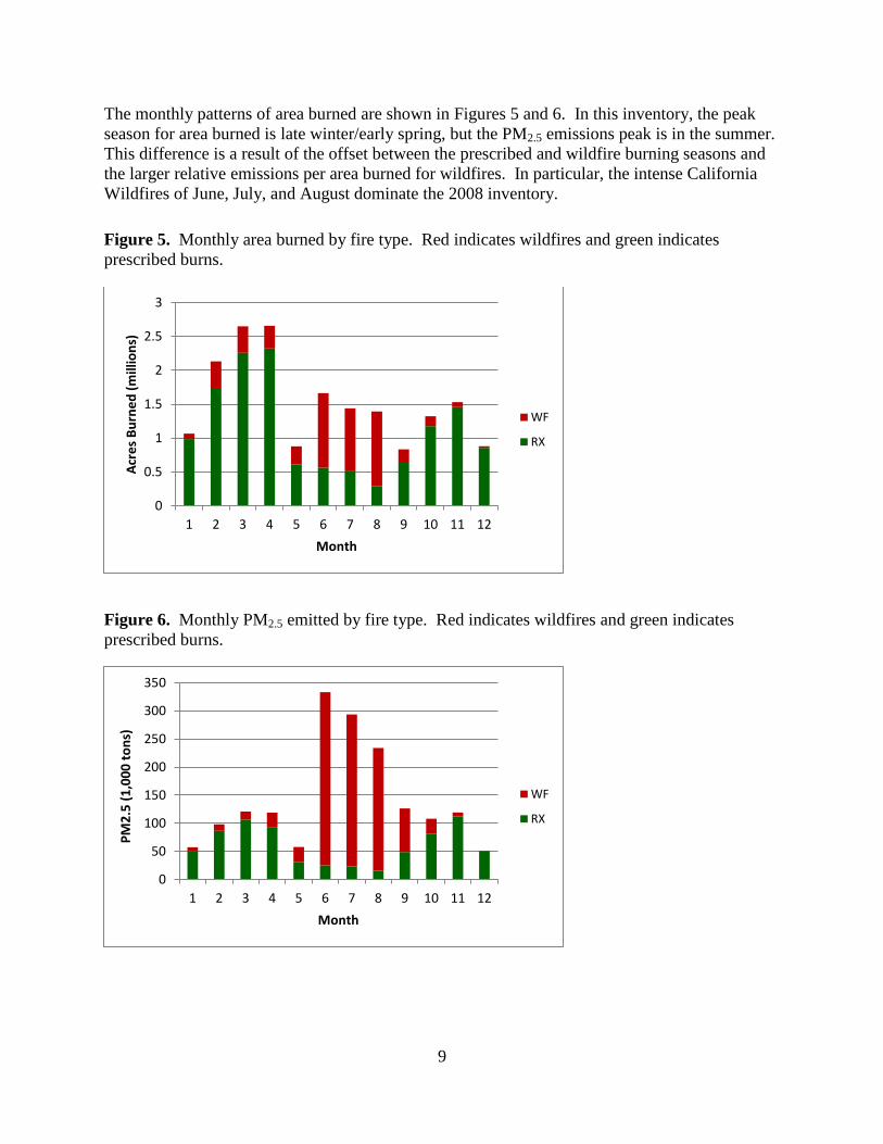
The monthly patterns of area burned are shown in Figures 5 and 6. In this inventory, the peak

season for area burned is late winter/early spring, but the PM2.5 emissions peak is in the summer.

This difference is a result of the offset between the prescribed and wildfire burning seasons and

the larger relative emissions per area burned for wildfires. In particular, the intense California

Wildfires of June, July, and August dominate the 2008 inventory.

Figure 5. Monthly area burned by fire type. Red indicates wildfires and green indicates

prescribed burns.

Figure 6. Monthly PM2.5 emitted by fire type. Red indicates wildfires and green indicates

prescribed burns.

0

0.5

1

1.5

2

2.5

3

1 2 3 4 5 6 7 8 9 10 11 12

Acr

es

Bu

rne

d (

mill

ion

s)

Month

WF

RX

0

50

100

150

200

250

300

350

1 2 3 4 5 6 7 8 9 10 11 12

PM

2.5

(1

,00

0 t

on

s)

Month

WF

RX

10

DISCUSSION

While we believe this work represents an improvement over past fire emissions inventories,

issues remain that can and should be addressed in future inventory development. Due to their

large effect on emissions totals, the duff consumption issues in Consume are perhaps most

important. Current versions of Consume calculate unrealistically high duff consumption for

fuelbeds with high duff depths for prescribed fires. To account for this issue in the current

inventory, an arbitrary cap based on expert judgment was applied. Future versions of Consume

are expected to address this concern.

Fire information from prescribed burns is lacking in the 2008 inventory. Some burn areas are

captured by MTBS, but estimates for most prescribed burn areas must rely on satellite data. To

produce a more accurate inventory, local ground-based data are needed. EPA typically depends

on state air quality agencies for NEI input data; however, only ten state air quality agencies

submitted both wildfire and prescribed burn emissions data to the NEI. Most state air quality

agencies do not track or collect such information. The state forestry agency may have this

information, but they are not part of the EPA NEI process. Federal fire activity databases are

another potential source of ground-based prescribed fire information. This federal data may or

may not be captured in state databases. EPA and federal and state agencies need to work

together to improve how fire information is reported to the NEI.

Emissions inventories of wildland fires remain highly uncertain. According to the Smoke

Emissions Model Intercomparison Project (SEMIP), critical areas of uncertainty include fire

activity information, fuel loading maps, and consumption.2 Further work is needed to validate

and improve all aspects of the smoke emissions modeling chain.

CONCLUSION

A new methodology, taking advantage of the latest versions of SmartFire and the BlueSky

framework, was used to produce a wildland fire emission inventory for the contiguous U.S. for

2008. We estimate that 16% of U.S. PM2.5 emissions come from wildfires and 12% of these

emissions come from prescribed burns. While there was far more prescribed fire area burned

than wildfire area, emissions from wildfires were higher. The historically large wildfires in

California represent 31% of the total estimated fire emissions. These totals may not be typical,

as wildfire activity exhibits strong inter-annual variability. Future inventories should focus on

improving known issues with duff consumption and acquiring additional information on area

burned from prescribed burns.

11

ACKNOWLEDGMENTS

We are grateful to all who offered suggestions and advice on the national scale processing of the

2008 NEI version 2 wildland fire emissions inventory. This includes (but is not limited to) all of

the members of the National Wildfire Coordinating Group Smoke Committee Retrospective-EI

Task Team (Mark Fitch, Nancy French, Jessica McCarty, Tom Moore, Susan O’Neill, Christine

Wiedinmyer, Gordon Andersson, and others), as well as state regulators from across the country.

All improvement in the NEI between version 1 and version 2 is due in large part to their efforts.

REFERENCES

1. Dentener, F.; Kinne, S.; Bond, T.; Boucher, O.; Cofala, J.; Generoso, S.; Ginoux, P.; Gong,

S.; Hoelzemann, J. J.; Ito, A.; Marelli, L.; Penner, J. E.; Putaud, J.-P.; Textor, C.; Schulz,

M.; G. R. van der Werf; Wilson, J. "Emissions of primary aerosol and precursor gases in

the years 2000 and 1750 prescribed data-sets for AeroCom", Atmospheric Chemistry and

Physics 2006, 6, 4321-4344. Available on the Internet at http://www.atmos-chem-

phys.net/6/4321/2006/acp-6-4321-2006.pdf.

2. Larkin, S.; Strand, T.; Martinez, N.; Rorig, M.; Krull, C.; Potter, B.; Drury, S.; Raffuse, S.;

Wheeler, N.; Craig, K.; Chinkin, L. "Uncertainties in fuels, consumption, plume rise and

smoke concentration calculations", Presented at the 3rd Fire Behavior and Fuels

Conference, Spokane, Washington, October 28, 2010

3. Prichard, S. J.; Ottmar, R. D.; Anderson, G. K. "Consume 3.0 user's guide"; Prepared by

the USDA Forest Service, Pacific Northwest Research Station, Seattle, WA. 2005.

4. Reinhardt, E. D.; Keane, R. E.; Brown, J. K. "First Order Fire Effects Model: FOFEM 4.0

user’s guide."; Forest Service General Technical Report INT-GTR-344, Prepared by the

U.S. Department of Agriculture. 1997.

5. Larkin, N. K.; O'Neill, S. M.; Solomon, R.; Raffuse, S.; Strand, T. M.; Sullivan, D. C.;

Krull, C.; Rorig, M.; Peterson, J.; Ferguson, S. A. "The BlueSky smoke modeling

framework", Int. J. Wildland Fire 2009, 18(8), 906-920 (STI-3784, doi:10.1071/WF07086).

6. The Fuel Characteristic Classification System (FCCS). USDA Forest Service, Web page of

the U.S. Forest Service, Fire and Environmental Research Applications Team, Seattle, WA,

2008. Available at: http://www.fs.fed.us/pnw/fera/fccs/.

7. Anderson, G. K.; Sandberg, D. V.; Norheim, R. A. "Fire Emission Production Simulator

(FEPS) user's guide version 1.0"; Prepared by the USDA Forest Service, Pacific Northwest

Research Station, Seattle, WA. 2004.

8. Eidenshink, J.; Schwind, B.; Brewer, K.; Zhu, Z.-L.; Quayle, B.; Howard, S. "A project for

monitoring trends in burn severity", Fire Ecology Special Issue 2007, 3(1), 3-21.

9. Monitoring Trends in Burn Severity (MTBS). Wildland Fire Leadership Council, Website

2012. Available at: http://www.mtbs.gov/.

12

KEY WORDS

Emission Inventory

SmartFire

BlueSky

Smoke

Wildfire

Prescribed Burn

PM2.5

NEI