Development of Spatial Mental Representations in an ... · programmer, the programming part of the...

Development of Spatial Mental Representations

in an Embodied Artificial Neural Network

Using Sequential and Egocentric Data

Master thesis by

Merijn Bruijnes

Development of Spatial Mental Representations in an Embodied

Artificial Neural Network Using Sequential and Egocentric Data

Master thesis by

Merijn Bruijnes

s0097519

17 August 2011

University of Twente

Faculty of Behavioral Sciences, Psychology

Department of Cognitive Psychology & Ergonomics

First supervisor: dr. Frank van der Velde

Second supervisor: dr. Matthijs Noordzij

2

Acknowledgments

Writing this thesis was a very pleasant process for me, largely due to the support of all

the people around me. I would like to thank a number of people in particular.

First, I would like to thank my supervisors, Frank van der Velde and Matthijs

Noordzij. They were enthusiastic about my ideas and gave me free reign on the project.

Without their help, this project would not have been successful and might not have

finished in time. A special thanks to Frank, for being available during the weekend near

the end of the project.

Next, I would like to thank a wonderful group of fellow students. I had a great time

during the long days (and sometimes nights) were we studied together in our little office.

Without your support, and the occasional coffee break, the completion of this thesis

would have taken a long time and most importantly, would not have been as satisfying.

Other people helped me during the project, in various ways. My little brother, Florian

Bruijnes, gave me a crash course in math, to revive my faded math skills. As I am no

programmer, the programming part of the project benefited greatly from the help of Koos

Mavrakis, who gave me some pointers when I was stuck. I am also very grateful to all the

people that proofread (parts of) my thesis. Thanks to Gerrit Bruijnes (my dad), Eva

Beltman, Alfons Laarman, and Lucas Meertens this thesis is of the current quality.

Finally, my entire family and all my friends were very helpful during this project in

that they allowed me to think aloud. Their questions and feedback helped me solidify my

ideas. Their interest in me as a person and my work as a student gives me great joy in

life.

3

Abstract

The current study investigated the development of spatial relations in an artificial neural

network. Design constraints and requirements for the artificial neural network were

formulated from literature, in an attempt to make the network psychologically and

neurobiologically plausible. Egocentric route information was taught to a network using

back propagation. The network was embodied in a Lego Mindstorms robot. The

(embodied) network successfully managed to navigate a learned maze. Using principal

component analysis to investigate the representations the network built, components for

direction and location were found. They hinted at preparation effects and the basis for an

emerging allocentric representation. No evidence for the ability to find novel routes was

found.

4

Table of contents

1. Introduction ..................................................................................................................... 7

1.1 Psychology and artificial intelligence ....................................................................... 7

2. Spatial Cognition .......................................................................................................... 10

2.1 Psychology .............................................................................................................. 10

2.2 Neuroscience ........................................................................................................... 14

2.3 Artificial cognition .................................................................................................. 17

3. Neural network models ................................................................................................. 20

3.1 Neural networks ...................................................................................................... 20

3.2 Spatial cognitive neural model for route information ............................................. 23

4. Methods......................................................................................................................... 25

4.1 Modeling the neural network .................................................................................. 25

4.2 The spatial environment .......................................................................................... 26

4.3 Training the network ............................................................................................... 27

4.4 Embodying .............................................................................................................. 28

4.5 Lane keeping ........................................................................................................... 31

4.6 Testing the network................................................................................................. 32

4.7 Network analysis ..................................................................................................... 32

5. Results ........................................................................................................................... 34

5.1 Virtual results .......................................................................................................... 34

5.2 Analog results ......................................................................................................... 34

5.3 Network analysis ..................................................................................................... 35

6. Discussion and conclusions .......................................................................................... 42

6.1 Theoretic demands from psychology ...................................................................... 42

6.2 Theoretic demands from neurophysiology ............................................................. 45

5

6.3 Model improvement ................................................................................................ 47

6.4 Embodied system .................................................................................................... 49

6.5 Practical implications and future directions ............................................................ 51

References ......................................................................................................................... 54

Appendix A: Dynamic field theory................................................................................... 59

Appendix B: Artificial neural networking and back propagation ..................................... 61

Appendix C: Guidance ...................................................................................................... 65

Guide to MemBrain ...................................................................................................... 65

Guide to code changes in BricxCC ............................................................................... 68

Guide to Lego Mindstorms ........................................................................................... 69

Building guide to Wobot ............................................................................................... 72

Appendix D: Neural network in MemBrain ..................................................................... 73

Appendix E: NXC code, algorithms ................................................................................. 74

Appendix F: NXC code, variables .................................................................................... 85

7

1. Introduction

Humans are very capable of finding their way in known and unknown environments. It is

such a natural activity for most that they do not even pay much attention to the task. They

just do and when they get lost, asking for directions generally solves the problem. A

helpful passerby gives a sequence of directions and we are able to form an idea of where

we are, where our goal is, and how to get there. It has been widely found that humans are

very flexible in completing various route finding tasks (e.g. Noordzij, Zuidhoek &

Postma, 2006). To complete such tasks, it is necessary to have some mental

representation of the spatial information. However, the nature of the representations

necessary for spatial tasks is still under debate (e.g. Burgess, 2006). This thesis tries to

model such spatial representations in an artificial system.

In this chapter, I first explain why it is useful for psychology to investigate artificial

systems performing human tasks. In the next chapter, an outline of the field is given, in

order to show where hiatus are and how they might be filled. The third chapter ends with

a description of an embodied artificial neural model that can perform a route-finding task.

1.1 Psychology and artificial intelligence

To understand why psychologists are interested in modeling artificial mental systems it is

important to consider where psychology came from. Psychology has its roots in ancient

philosophy and medicine. Hippocrates started describing natural causes of psychological

conditions, gave clear descriptions of many behavioral problems, and formulated theories

of temperament and motivation. These theories were very influential in science and

though science has since moved on, some of Hippocrates‟ ideas are still used in

8

contemporary language (Hothersall, 2004, p.18). Behaviorism (focus on behavior),

combined with some introspection, were the main psychologists tools for the bulk of the

psychological history. It provided us with some great theories of mind, but was largely

limited to behavior and did not reveal much of the inner workings of the brain.

Only recently, tools have become available that allow for in vivo measurements of

electrical or metabolic changes, which are related to brain activity. Neuroscientific tools

such as electroencephalography (EEG), functional magnetic resonance imaging (fMRI),

and magnetoencephalography (MEG) enable us to probe the activation patterns of the

working brain. These techniques generally show what areas of the brain are active during

some task, but they do not easily show how these active brain areas solve some task or

produce behavior. Initiatives, such as knife-edge scanning microscopy for imaging and

reconstruction of three-dimensional anatomical structures, give extremely detailed (sub-

micron resolutions) neuroanatomical maps of neurons, their interconnectiveness, and

their larger scale structures (Mayerich, Abbott, & McCormick, 2008). These impressive

neuroscientific feats provide us with a wealth of information on the anatomy of the brain.

However, to make a translation from physiology to cognition we need more than

knowledge of the neuroanatomy and theories of behavior. We need a way to investigate

the mechanisms that generate intelligence and cognition, which is exactly the focus of

artificial intelligence research. This is where neuroscience, artificial intelligence, and

psychology meet. We all want to understand the structural (neural) elements that root

cognition, perception, and other psychological constructs and we all need models to

accomplish it (van der Velde, 2010).

9

Now that it is clear why psychologists are interested in modeling artificial cognition

systems, it is time to give a, far from complete, overview of the work done so far in this

multidisciplinary field. I focused on spatial cognition and in particular on the

representations needed to complete a spatial route-finding task. First, spatial cognition

was investigated from the psychological and neuroanatomical view. This yielded some

constraints to which a psychological and neurological plausible artificial route finding

system should adhere. With such constraints in mind, artificial neural models were

investigated leading to an artificial neural network that is able to perform a route-finding

task in a psychological and neurological plausible way.

10

2. Spatial Cognition

This chapter presents theoretical background on spatial cognition. The goal is to

formulate a set of design constraints or guidelines for an artificial neural network.

Psychological and neurobiological literature is discussed, after which some examples

from artificial intelligence are presented.

2.1 Psychology

The cognitive mechanisms involved during navigation center on the creation, retrieval,

and application of spatial representations. The factors involving differences between

spatial representations were summed up aptly in four factors by Taylor, Brunyé, and

Taylor: “The nature of […] spatial mental representations may vary as a function of at

least the following: extent of experience […], nature of experience […], environmental

scale and complexity […], and individual differences” (p.2, Taylor, Brunyé, & Taylor,

2008). These factors relate to human cognition. This thesis, however, will describe an

embodied artificial neural model that can perform a route-finding task. Since the goal is

to create an artificial system that is rooted in (human) cognition, these human factors will

have to be taken into account.

Human spatial cognition seems to depend on at least two distinct spatial

representations: egocentric and allocentric representations (Burgess, 2006). Egocentric

and allocentric spatial representations differ in their frame of reference. In an egocentric

frame of reference, all objects or locations are represented in relation to the observer. In

an allocentric frame of reference, however, objects or locations are represented

11

independent of the observer, thus in object-object or location-location relations (e.g.

Burgess, 2006; Zaehle, Jordan, Wüstenberg, Baudewig, Dechent, & Mast, 2007).

Burgess (2006), in an opinion piece, summed up behavioral data, which suggests that

both representations are products of distinct systems. These two systems can operate

separately but they can also cooperate. As an example of separation, experiments by

Waller and Hodgson (2006) showed that the spatial cognitive system is able to switch

between representations. They showed participants an array of objects briefly, then

rotated the participant and asked them to point towards an object. An increase in pointing

error variation occurred after 135° of rotation but not after 90° or less. According to the

authors, this indicates a switch from one representation to another instead of a slow

compromise of one representation (Waller & Hodgson, 2006). This seems to indicate that

both systems can operate separately. However, the systems clearly have to work together.

For more supporting empirical evidence, please refer to Wang and Spelke (2000) or

Burgess (2006).

Allocentric representations are more suitable for long-term storage, as it is likely that

the body will have moved between presentation and recall. As imagery and sensory

perception are egocentric by nature, every time an allocentric representation is created or

used, a translation has to be made to and from egocentric representations. This also holds

true when allocentric information is used for action oriented (and thus egocentric)

representations (Burgess, Becker, King, & O‟Keefe, 2001; Burgess, 2006). All this is of

importance because this thesis will focus on egocentric representations developed during

or for a route-finding task. Neuropsychological studies have shown that egocentric

representations can occur separate from allocentric representations (e.g. Burgess, Becker,

12

King, & O‟Keefe, 2001). This means that an artificial system that can form (only)

egocentric representations is rooted in (neuro)psychological reality. However, it seems

important for such an egocentric artificial system to be compatible with an allocentric

artificial system (more on this in the discussion).

Denis and Zimmer (1992) showed spatial mental representations are similar, whether

they are built up from visual experience or from spatial descriptions. Humans are

consistently found to be capable of building usable spatial representations from simple

descriptions that contain some form of spatial information (e.g. Cocude, Mellet, & Denis,

1999; Noordzij & Postma, 2005; Noordzij, Zuidhoek, & Postma, 2006). The mechanism

that builds and uses a mental spatial representation appears to be very flexible. For

example, consider the mental spatial representation that can be built from a route

description or a survey description. A route description describes the environment in

egocentric clues, such as „go left at the bakery‟. A survey description gives information

about the environment in an allocentric manner (e.g. the bakery is to the north of the

zoo). After learning a route or a survey description, the same tasks (e.g. guessing the

distance between two points, or verifying first person perspective statements after

learning a layout) can be completed (e.g. Noordzij, & Postma, 2005). Interestingly they

later found that blind people perform better at a spatial task after listening to a route

description compared to a survey description. This was even true when the spatial task

explicitly favored a survey description (Noordzij, Zuidhoek, & Postma, 2006). Blind

people rarely use survey descriptions (e.g. a map) and mainly rely on route descriptions

to get around. At least for spatial information, this implies that the mechanism that builds

13

a spatial mental representation benefits if the spatial description is given in a familiar or

consistent way.

To understand the flexibility of spatial mental representations further, it is important

to consider the goals under which the representations are formed or used. Without a goal,

one would be wandering around aimlessly. It might not be possible to not have a goal;

even if one is wandering around aimlessly, it might be exactly the fulfillment of the goal

„wandering around aimlessly‟. Also, consider the example given earlier; a mental spatial

representation built from the description of a route or survey can be used to complete the

same tasks (Noordzij, & Postma, 2005). During training, the goal might be composing an

elaborate mental spatial model, for example with the intention to do well on a test. Later

the spatial knowledge acquired might be used in fulfilling the goal of getting to a location

as quickly as possible (e.g. Maguire et al., 2000). Goals seem sufficiently important to

address them explicitly in the embodied artificial neural model, which is discussed later

in this thesis.

Besides selecting a learned route, it is also possible to infer a novel route between

two visited points. For example, if there are three points (A, B, C) and the routes between

A-B and B-C are known, it is easy to go from A to C via B. It is also possible to take

shortcut A-C, thus inferring a novel route (see figure 1). Humans are capable of

computing such novel routes, however, only when there are landmarks present along the

routes to guide them (Foo, Warren, Duchon, & Tarr, 2005). The capability of the

embodied artificial neural model to compute a novel route is discussed later in this thesis.

14

Figure 1: Three destinations (A, B, C). Two learned paths (A-B and B-C) leave one novel

route to be discovered (A-C).

Summarizing, we can already specify some of the requirements the artificial neural

network should meet. For the artificial neural network to be an approximation of how

humans build and use spatial mental representations, it must:

(1) Consist of separate, but closely intertwined, systems for different spatial reference

frames;

(2) Benefit from a spatial description given in a familiar or consistent way during

training;

(3) Make use of goals in building and using a spatial mental representations;

(4) Be capable of selecting familiar routes and computing novel routes.

2.2 Neuroscience

The questions of what brain areas are involved in spatial cognition, and with how many

neurons, are difficult to answer precisely, yet they are important for an (artificial) model

of spatial cognition. Involvement of brain areas was found to vary over spatial tasks and

15

the representations required. Zaehle and colleagues (2007) investigated the difference

between an egocentric and an allocentric frame of reference in an fMRI study. They

found that the processing of egocentric spatial relations caused activation in the medial

superior–posterior areas, whereas allocentric spatial coding seemed to require an

additional involvement of the right parietal cortex, the ventral visual stream and the

hippocampal formation (Zaehle, Jordan, Wüstenberg, Baudewig, Dechent, & Mast,

2007). This suggests that in the human spatial cognitive system the egocentric spatial

coding only requires a subsystem of the entire processing resources needed for an

allocentric spatial coding task. Note, however, that Zaehle et al. used novel spatial stimuli

in their experiment.

Mellet et al. (2000) compared brain activation in route and survey navigation tasks,

using pre-learned spatial information, with PET. It seems logical that route navigation

would have an egocentric frame of reference, while survey navigation would use

allocentric representations. They found that the tasks shared some brain activation, but

also caused activation in distinct areas. The right hippocampus was active in both survey

and route tasks, and therefore might hold the neural equivalent of a dual-perspective

representation. During a route navigation task, additional activity was found in the

parahippocampal gyrus. This suggests, this area is used when there are landmarks in the

environment (Mellet et al., 2000). Similar results were found when imaging the active

brain areas during mental replay of navigation (Ghaem et al., 1997).

Note that this seems opposite to what the Zaehle study found. However, Zaehle used

novel stimuli while Mellet et al. (2000) and Ghaem et al. (1997) used previously learned

stimuli. In addition, the tasks differed; Zaehle et al. (2007) used a spatial visual judgment

16

task, while Mellet and colleagues (2000) asked participants to imagine navigating an

environment. Therefore, the discrepancy might be due to the difference in task or a

difference between learning and recovering spatial information.

Both findings, however, do seem to indicate that there are distinct, albeit closely

related, systems for different forms of spatial information. In other words, there seems to

be neuroanatomical evidence that egocentric and allocentric spatial information are

processed in distinct areas of the brain. This gives some legitimacy to a model that is

fairly specific for one spatial task (i.e., there might be different models for different

tasks). However, a spatial model should be versatile and with minor adjustments or

additions capable of performing different tasks.

The structure of the cortex, and that of the bordering hippocampi, is highly regular.

There are distinct layers of neurons stacked on top of each other. Across these layers are

small vertical columns spanning the layers. Both layers and columns are strongly intra-

and interconnected. Further, neurons within a column generally have similar response

characteristics and it is suggested that they operate as a (functional) group. Finally,

similar cortical circuits are found all over the cortex (e.g. van der Velde, 2010). This

pushes us further to try to find simple and versatile mechanisms of cognition that are like

building blocks. One such neural circuitry building block might not be powerful enough

to perform anything but the most basic form of cognitive operations, but more blocks

together might show more complex computing power.

The size of brain areas can vary as a result of high (navigational) skill dependency.

In an often-quoted study by Maguire and colleagues (2000), London taxi drivers were

found to have bigger posterior hippocampi than controls. Also, the amount of time spend

17

as a taxi driver correlated positively with posterior hippocampal volume. This coincides

nicely with the idea that this area is responsible for storing spatial information about the

environment (Maguire et al., 2000). It might also imply that the mechanism responsible

for building and using spatial mental representations can recruit more neurons if

necessary, which is of importance to keep our (artificial) mental model rooted in biology.

Summarizing we can specify some more requirements an artificial neural network

should meet. In order for an artificial neural network to maintain a root in biology, it

should follow these guidelines:

(5) The model can be (single) task specific;

(6) The model should have a simple mechanism to produce cognition;

(7) These mechanisms should be like building blocks;

(8) It should be possible to change or combine these simple basic building blocks to

change their function.

2.3 Artificial cognition

Now that it is clear what the spatial mental model and the artificial neural network should

be able to do, it is time to review what artificial models are out there and which we might

use. First, some descriptions of mental models are given and from these models, a spatial

mental model that can represent route information emerges.

Artificial intelligence (AI) and cognitive modeling provide an important opportunity

for improving our understanding of human cognition. Traditional psychology uses human

behavior as the main source of data while neuropsychology mainly studies the workings

of neurons and neuronstructures. However, to understand intelligence and cognition truly,

18

we also need to understand the mechanisms that generate them. To accomplish this we

can try to model such mechanisms, while of course adhering to the constraints that came

from psychological and neuroscientific research. Modeling cognition forces us to

acknowledge factors that might have stayed hidden otherwise.

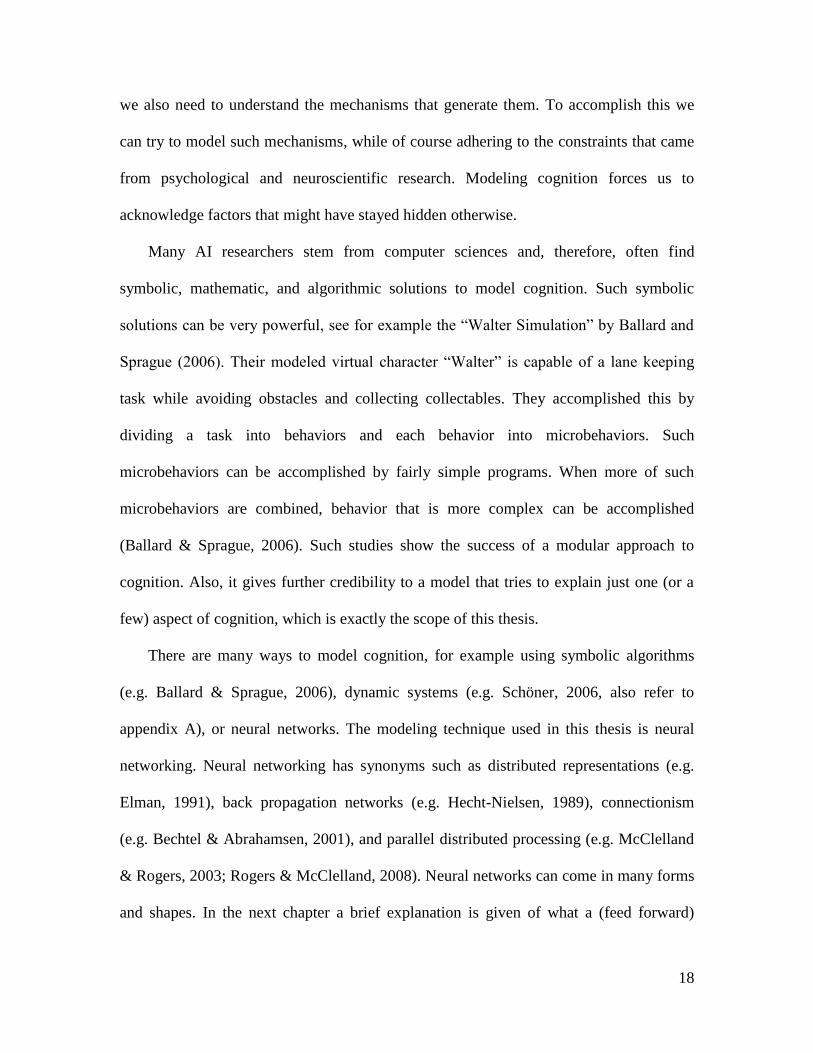
Many AI researchers stem from computer sciences and, therefore, often find

symbolic, mathematic, and algorithmic solutions to model cognition. Such symbolic

solutions can be very powerful, see for example the “Walter Simulation” by Ballard and

Sprague (2006). Their modeled virtual character “Walter” is capable of a lane keeping

task while avoiding obstacles and collecting collectables. They accomplished this by

dividing a task into behaviors and each behavior into microbehaviors. Such

microbehaviors can be accomplished by fairly simple programs. When more of such

microbehaviors are combined, behavior that is more complex can be accomplished

(Ballard & Sprague, 2006). Such studies show the success of a modular approach to

cognition. Also, it gives further credibility to a model that tries to explain just one (or a

few) aspect of cognition, which is exactly the scope of this thesis.

There are many ways to model cognition, for example using symbolic algorithms

(e.g. Ballard & Sprague, 2006), dynamic systems (e.g. Schöner, 2006, also refer to

appendix A), or neural networks. The modeling technique used in this thesis is neural

networking. Neural networking has synonyms such as distributed representations (e.g.

Elman, 1991), back propagation networks (e.g. Hecht-Nielsen, 1989), connectionism

(e.g. Bechtel & Abrahamsen, 2001), and parallel distributed processing (e.g. McClelland

& Rogers, 2003; Rogers & McClelland, 2008). Neural networks can come in many forms

and shapes. In the next chapter a brief explanation is given of what a (feed forward)

19

neural network is and what it can do (cf. appendix B, Bechtel & Abrahamsen, 2001, and

Zeidenberg, 1990). Two basic forms will be elaborated on further, the simple recurrent

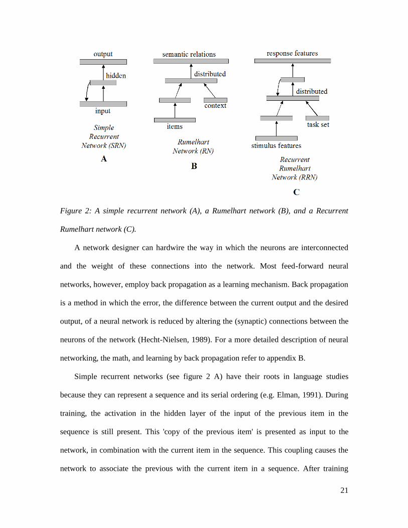
network (e.g. Elman, 1991), and the Rumelhart network (e.g. McClelland & Rogers,

2003); see figure 2 and the next chapter for the distinction.

20

3. Neural network models

In this chapter, some existing artificial neural network models are discussed. A

combination of existing models leads to a model that can learn and represent a route.

3.1 Neural networks

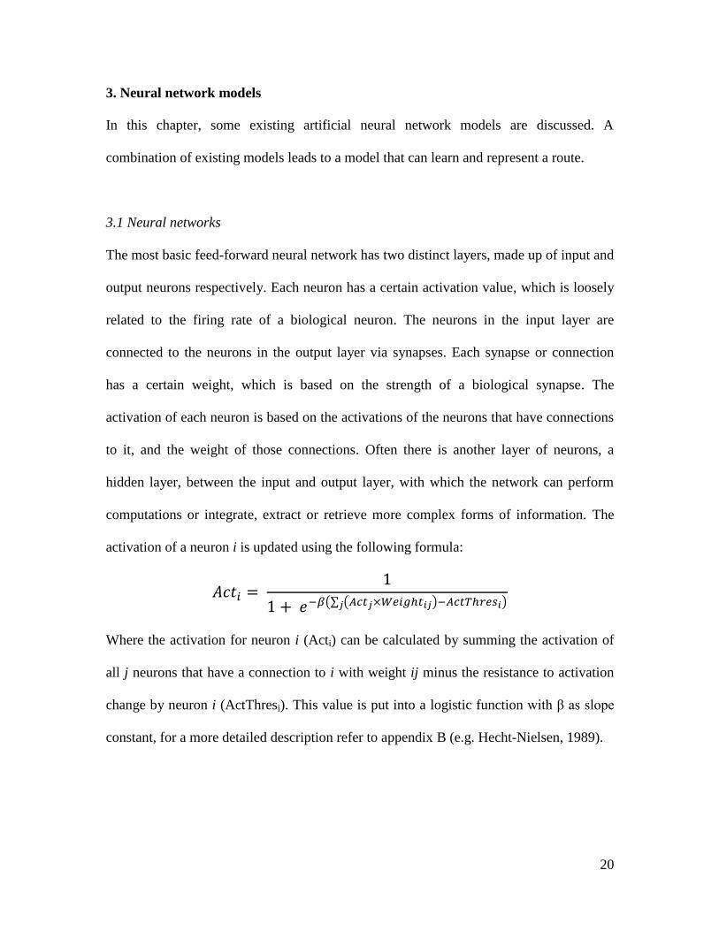
The most basic feed-forward neural network has two distinct layers, made up of input and

output neurons respectively. Each neuron has a certain activation value, which is loosely

related to the firing rate of a biological neuron. The neurons in the input layer are

connected to the neurons in the output layer via synapses. Each synapse or connection

has a certain weight, which is based on the strength of a biological synapse. The

activation of each neuron is based on the activations of the neurons that have connections

to it, and the weight of those connections. Often there is another layer of neurons, a

hidden layer, between the input and output layer, with which the network can perform

computations or integrate, extract or retrieve more complex forms of information. The

activation of a neuron i is updated using the following formula:

Where the activation for neuron i (Acti) can be calculated by summing the activation of

all j neurons that have a connection to i with weight ij minus the resistance to activation

change by neuron i (ActThresi). This value is put into a logistic function with β as slope

constant, for a more detailed description refer to appendix B (e.g. Hecht-Nielsen, 1989).

21

Figure 2: A simple recurrent network (A), a Rumelhart network (B), and a Recurrent

Rumelhart network (C).

A network designer can hardwire the way in which the neurons are interconnected

and the weight of these connections into the network. Most feed-forward neural

networks, however, employ back propagation as a learning mechanism. Back propagation

is a method in which the error, the difference between the current output and the desired

output, of a neural network is reduced by altering the (synaptic) connections between the

neurons of the network (Hecht-Nielsen, 1989). For a more detailed description of neural

networking, the math, and learning by back propagation refer to appendix B.

Simple recurrent networks (see figure 2 A) have their roots in language studies

because they can represent a sequence and its serial ordering (e.g. Elman, 1991). During

training, the activation in the hidden layer of the input of the previous item in the

sequence is still present. This 'copy of the previous item' is presented as input to the

network, in combination with the current item in the sequence. This coupling causes the

network to associate the previous with the current item in a sequence. After training

22

(using back propagation) the simple recurrent network can 'predict' the next item in the

sequence (Elman, 1991). This ability might be useful as a building block for route finding

skills. The simple recurrent network could report the next step, the direction to turn, in a

route that it knows. However, it cannot discriminate between (overlapping) routes.

Figure 3: The proposed neural network that can model the spatial route information. The

network consists of four layers. The number of neurons is displayed for each group. The

top layer is the input layer where three groups serve as input for the network: the current

location, the destination, and a copy of the first hidden layer (hidden recurrent). This

copy of the previous first hidden layer activation (recurrent) and the current location are

fed into the first hidden layer. The first hidden layer feeds a copy of its activation, via the

recurrent connections, to the hidden recurrent layer. It also feeds to a second hidden

layer that combines the goal and the input. In the output layer the (turning) decision

necessary to reach the destination, will become active.

23

A Rumelhart network (see figure 2 B) can represent context and as such it might

discriminate between sequences, grammatical context, or perhaps routes as in our case.

For example, in a language case the network could learn the difference between 'canary

can fly' and 'canary has wings'. When the same input is given, 'canary', the network can

distinguish between outputs „fly‟ or „wings‟ because of the context, either 'can' or 'has'

(McClelland & Rogers, 2003). However, the Rumelhart network is not capable of

learning sequential information (such as a route).

3.2 Spatial cognitive neural model for route information

A recurrent Rumelhart network (see figure 2 C) is a combination of a simple recurrent

network and a Rumelhart network, combining the ability to represent sequential

information and context. Therefore, a recurrent Rumelhart network might be able to

learn, represent, and distinguish between different (overlapping) routes. See figure 3 for

the network I developed. During the learning of routes, the input is the sequence of

locations along the route and the corresponding output of directions. The recurrent nature

of the network builds the temporal order representation of the items. The context is the

goal (the final location), which is continuously presented to the context neurons (called

task set in figure 2 C). This results in a network that represents the sequence of directions

of routes and can distinguish between different routes using the goal or destination of the

route. After learning, a destination is presented to the network as a goal and the first

location as the input. The network now generates the direction to get to the next location

on the route. When this next location is presented as input the network generates the next

following direction. These steps continue until the goal is reached. Additionally, it is

24

possible to start midway in a learned route, as long as the „start‟ location is in one of the

learned routes to the goal. Starting midway in a route comes with the additional

constraint that the direction an embodied network (e.g. robot) is facing is compliant with

the direction of the route.

Now that an artificial spatial (route) neural model is presented (see figure 3), I will

repeat the requirements stipulated earlier from the psychological and neuroanatomical

review. The described neural network was embodied and tested against the requirements,

see chapter 4. The results (chapter 5) are discussed in the discussion, chapter 6. In order

for the artificial neural network to be a possible approximation of how humans build and

use spatial mental representations, it must:


frames;


training;



Moreover, in order for an artificial neural network to maintain a root in biology it should

follow these guidelines:


(6) The model should have a simple mechanism to produce cognition;

(7) These mechanisms should be like building blocks;



25

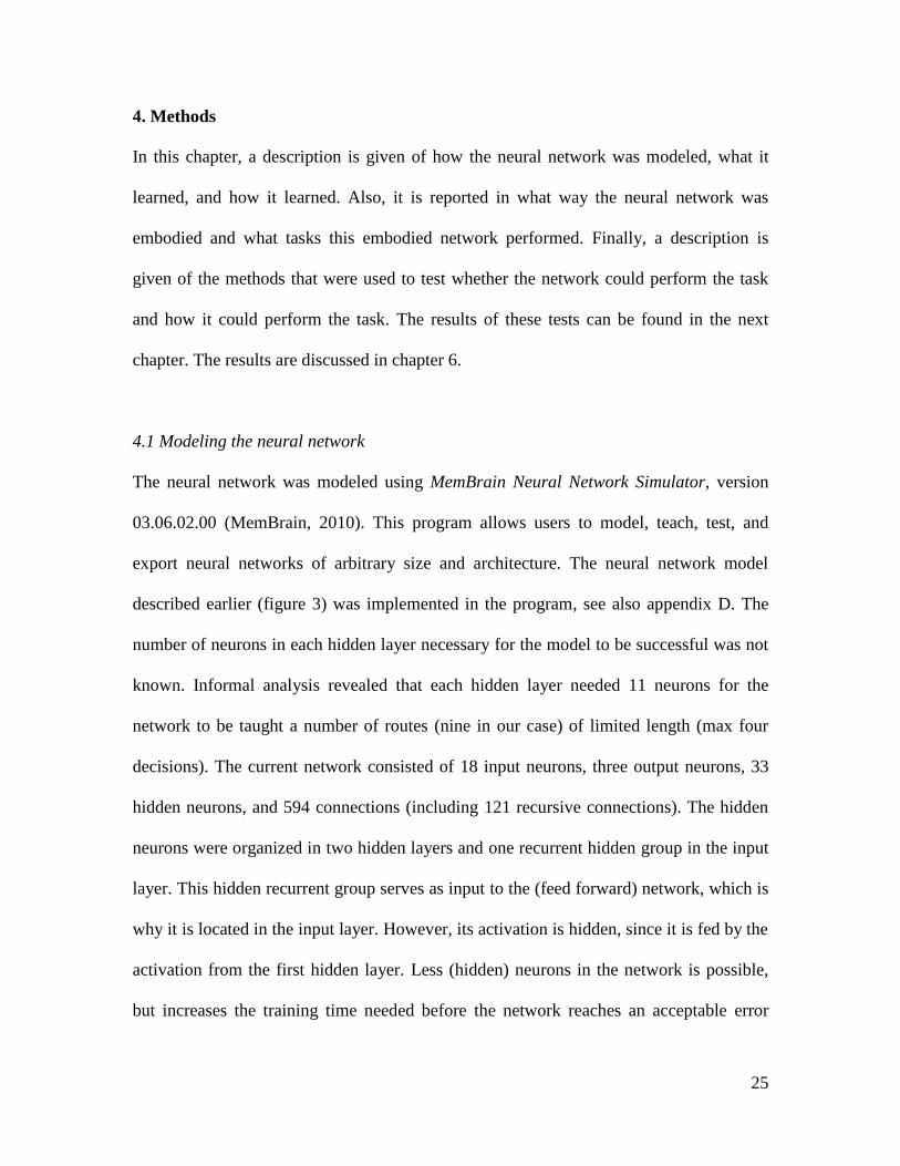
4. Methods

In this chapter, a description is given of how the neural network was modeled, what it

learned, and how it learned. Also, it is reported in what way the neural network was

embodied and what tasks this embodied network performed. Finally, a description is

given of the methods that were used to test whether the network could perform the task

and how it could perform the task. The results of these tests can be found in the next

chapter. The results are discussed in chapter 6.

4.1 Modeling the neural network

The neural network was modeled using MemBrain Neural Network Simulator, version

03.06.02.00 (MemBrain, 2010). This program allows users to model, teach, test, and

export neural networks of arbitrary size and architecture. The neural network model

described earlier (figure 3) was implemented in the program, see also appendix D. The

number of neurons in each hidden layer necessary for the model to be successful was not

known. Informal analysis revealed that each hidden layer needed 11 neurons for the

network to be taught a number of routes (nine in our case) of limited length (max four

decisions). The current network consisted of 18 input neurons, three output neurons, 33

hidden neurons, and 594 connections (including 121 recursive connections). The hidden

neurons were organized in two hidden layers and one recurrent hidden group in the input

layer. This hidden recurrent group serves as input to the (feed forward) network, which is

why it is located in the input layer. However, its activation is hidden, since it is fed by the

activation from the first hidden layer. Less (hidden) neurons in the network is possible,

but increases the training time needed before the network reaches an acceptable error

26

level. More on the training of the network later, first the spatial environment that was

taught will be discussed.

4.2 The spatial environment

The (embodied) network will navigate a grid-like maze. For this thesis a maze with nine

intersections or positions was used, however an arbitrary number of positions can be used

if enough neurons are available in the neural net. Intersection, position, and location are

used as synonyms throughout this thesis. Each position has a number and positions

double as destinations. As the (embodied) network traverses through the maze, it makes a

turning decision at each intersection (even if there is only one possibility). Thus, a route

(e.g. to P5) consists of a sequence of positions (e.g. P1, P4, P7, P8, P5) with the

corresponding directions to turn (e.g. straight, straight, right, right).

Figure 4: The maze that was used to train de neural network. It contains nine positions

(or intersections), the grey areas, named 1 through 9. The start point of each route is the

X, facing toward position 1. Four blockades are in place, so that each position can only

be reached via one route. More than one choice in direction is possible at two

intersections (P1 and P8).

27

Table 1: The routes to the various goals and the corresponding directions at the positions

during the route (S = straight, R = right, and L = left). Also, the color code for each

goal/position is shown.

Goal Route Directions Color code for goal position

P1 P1 - Yellow, Green, Red

P2 P1, P2 R Yellow, Red, Green

P3 P1, P2, P3 R, S Green, Yellow, Red

P4 P1, P4 S Green, Red, Yellow

P5 P1, P4, P7, P8, P5 S, S, R, R Red, Yellow, Green

P6 P1, P2, P3, P6 R, S, L Red, Green, Yellow

P7 P1, P4, P7 S, S Yellow, Green, Yellow

P8 P1, P4, P7, P8 S, S, R, S Yellow, Red, Yellow

P9 P1, P4, P7, P8, P9 S, S, R, S Green, Yellow, Green

Further, in this particular case each route started at the same position, at the X in

figure 4. Some “roads” were closed to decrease the complexity of the maze, as fewer

routes are possible, see figure 4. Also, this ensures that the routes are highly overlapping.

A route was constructed to each location, see table 1 for all the routes and their

corresponding directions.

4.3 Training the network

The routes and directions from table 1 were taught to the network using back

propagation. Back propagation is a method in which the error, the difference between the

28

current output and the desired output, of a neural network is reduced by altering the

(synaptic) connections between the neurons of the network (Hecht-Nielsen, 1989). Before

training starts, the weights of the links in the untrained network are randomized. In

training, there are two phases for each stimulus, the feed forward and the back

propagation. The first input of a sequence is presented as input to the network. The

network feeds this input forward and produces an output, which is likely to be far from

the desired output. This difference between desired and actual output is designated as the

error. Next, the contribution to the error is calculated for each neuron in the previous

layer and the weight of its connection is altered accordingly. This back propagation of

error is carried out for each layer in the network. When the back propagation is complete,

the next item in the stimulus set is presented as input and the cycle repeats (cf. appendix

B, Hecht-Nielsen, 1989).

Back propagation is a powerful learning tool. However, presenting the entire set of

stimuli once is often not enough to get a well-trained network, especially if the stimulus

set is large. After little training, the network will continue to make errors. It is difficult to

predict how many training cycles are necessary to get adequate network performance.

This is solved by setting an error level that the network has to reach. Training continues

until this level is reached. The time (amount of training cycles) to reach the desired error

level varies, as the network is randomized before training.

4.4 Embodying

The (spatial) neural network was embodied in the Lego Mindstorms platform. This

platform includes a small processing unit, several sensors, and actuators. The robot built

29

with this platform, see figure 5, was named Wobot (Wayfinding Robot). The processing

power and memory of the platform is limited therefore, it was not feasible to teach the

neural network using the processor in the robot. This means Wobot cannot drive around

and learn new things. It was also considered whether a Bluetooth link to a PC could be

used to exchange real-time sensor data from the robot to the neural network and issue

real-time motor commands from the network to the robot. Such a real-time link proved

very troublesome, so a more proof-of-concept approach was taken. Please refer to the

appendix C for a more detailed description of the Mindstorms platform and its limitations

(also cf. Toledo, 2006). The neural network was trained on a PC and the trained network

was uploaded to the robot. Thus, to teach Wobot a new route a new (trained) network has

to be uploaded. The robot is capable of supplying the network with sensor data and

computing the output of the network. The network output, in turn, influences Wobot‟s

motors. This cycle was real-time. The exact procedures of uploading a neural network,

along with the programming code used to embody the network, can be found in appendix

C, E, and F.

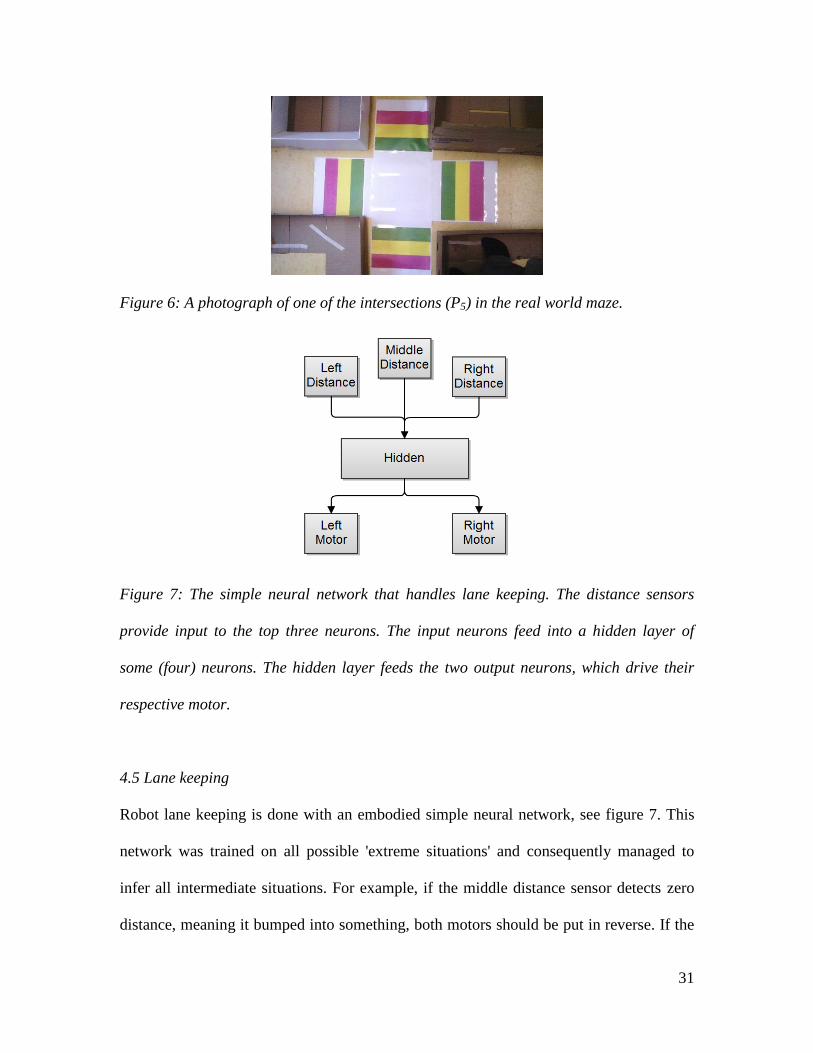
Wobot‟s sensor array consists of three ultrasonic distance sensors for lane keeping

and one down facing color sensor for recognizing locations. How lane keeping is

implemented will be discussed later, first the way Wobot recognizes where it is will be

explained. An efficient way for a robot (or for an animal for that matter) to determine its

location, is using vision. Unfortunately, the Lego Mindstorms platform does not include a

camera. It does, however, include a rudimentary color sensor that can recognize a meager

six colors (barely, as I will explain later). As mentioned earlier, the used maze has nine

locations that need recognizing, so simply assigning a color to each location would lead

30

to ambiguity as some colors are assigned to more than one location. This was solved by

using a three-color barcode that identifies a location, see figure 6 and table 1. As you can

see from figure 6, red looks more like pink, this is intentional and because the color

sensor detected red more reliable, if the actual color was pink rather than red. A signaling

color (white) was used as a signal in the software that a route was coming up; this means

that if the sensor detected the signaling color the robot would start keeping count of what

colors it saw. When the signaling color was detected again, the color code was finished

and the code could be looked up. The resulting location was fed to the neural network to

get a direction. In addition, the signaling color prevents interference from the color of the

ground, as the ground color might be used in a color code.

Figure 5: The Lego Mindstorms robot, which I dubbed Wobot (for Wayfinding Robot).

From top to bottom of the picture, the following components can be identified. The white

box, called the brick, houses the processor and other electronics. To the left and right the

tracks are visible, both powered by their own motor. Below the brick there are three

distance sensors visible, pointed forward and slightly to the left and right. At the bottom

of the image a color sensor is visible, it is facing down.

31

Figure 6: A photograph of one of the intersections (P5) in the real world maze.

Figure 7: The simple neural network that handles lane keeping. The distance sensors

provide input to the top three neurons. The input neurons feed into a hidden layer of

some (four) neurons. The hidden layer feeds the two output neurons, which drive their

respective motor.

4.5 Lane keeping

Robot lane keeping is done with an embodied simple neural network, see figure 7. This

network was trained on all possible 'extreme situations' and consequently managed to

infer all intermediate situations. For example, if the middle distance sensor detects zero

distance, meaning it bumped into something, both motors should be put in reverse. If the

32

left distance sensor detects decreasing distance, the right motor is slowed down, thus

turning right. Lane keeping did is switched off during a turn and switched back on when

the turn is complete.

4.6 Testing the network

Testing whether the neural network architecture works (after training) can be done

virtual, by presenting input to the network and check whether the output is as expected.

Also, it is possible to test analog, embodied, in the real world. Both ways of testing were

done, albeit an analog test was executed only with one version of the neural network (as a

proof of concept). The results of the tests are presented in the results chapter.

4.7 Network analysis

The successful completion of the tests shows whether a neural network has managed to

build some representation with which it can solve the spatial navigation task. It is more

interesting, however, to see how the network managed to solve its task. To reiterate the

point made in the introduction, in order to understand cognition it is necessary to

understand the mechanisms behind cognition. One way to approach this is to understand

the way in which an artificial neural network managed to solve a task. The solution to a

task an artificial neural network found might not at all resemble the way a biologic neural

network solves the same task. Nonetheless, investigating the artificial neural network can

give us an idea how a biological system might work.

To investigate how the network represents the spatial environment, we can directly

observe the internal state of the network as it makes decisions. In other words, the

33

activation of the (hidden) neurons can be scrutinized for every (environmentally) possible

input. This shows how all possible states are represented in the network. However,

simply looking at the hidden neuron activation patterns might not reveal much, as this

would be a diagram with as many dimensions as hidden neurons. Therefore, I conducted

a rotation of the axes of the dimensions, using principal component analysis (PCA). This

technique can be used to find the axis along which the most variance occurs. This means

that it can reveal the structure of the data as it is represented in the neural network (see

also Elman, 1991, & Kutner, Nachtheim, Neter, & Li, 2005).

To obtain the data for this analysis, each position in every route was presented to the

trained network and the activation value of all neurons was exported for each of these

instances. This dataset, with essentially as many dimensions as neurons, was imported in

a statistical program (SPSS18). There the covariance matrix is calculated to find the

principal components and their eigenvalues. The first few, relevant, components are

investigated further. These most relevant components serve as „viewpoints‟ from which

the data can be observed in the most informative way. An interpretation is given for the

relevant components.

34

5. Results

In this chapter, the results are summed up. The results are discussed in detail in the next

chapter.

5.1 Virtual results

For the current spatial neural network, an error level of 1e-7 was reached after about 100

training cycles. This training provided already adequate network performance. The

maximum error level for the network in this thesis, however, was set to 1e-10, which

generally took over 6.000 training cycles to reach. The 1e-10 threshold was chosen as it

makes errors during testing extremely unlikely. Also, because processing power was not

an issue. No errors were found, the network performed perfectly accurate on all learned

routes.

5.2 Analog results

The spatial neural network performed equally well in the embodied environment. There

were many instances where the robot provided erroneous data to the network, which led

to a failure to reach the goal location.

The embodiment of the network did not produce insurmountable problems, for the

programming code refer to appendix E and F. The platform, however, did come with a

troublesome color sensor. It was very difficult to make it read colors correctly. The

sensor made many errors, which lead to erroneous data being fed to the neural network

(see appendix C for a more detailed description of the limitations of the Lego Mindstorms

35

platform). Whenever the color sensor worked appropriately, however, Wobot was

consistently able to find its way in the maze.

5.3 Network analysis

The PCA of the spatial neural network revealed 20 components from which four are

relevant, see figure 8. The four relevant components combined, explain 84,9% of the

variance.

Figure 8: The principal components found and their respective eigenvalues.

36

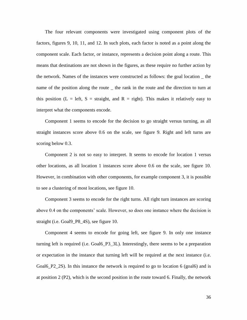
The four relevant components were investigated using component plots of the

factors, figures 9, 10, 11, and 12. In such plots, each factor is noted as a point along the

component scale. Each factor, or instance, represents a decision point along a route. This

means that destinations are not shown in the figures, as these require no further action by

the network. Names of the instances were constructed as follows: the goal location _ the

name of the position along the route _ the rank in the route and the direction to turn at

this position (L = left, S = straight, and R = right). This makes it relatively easy to

interpret what the components encode.

Component 1 seems to encode for the decision to go straight versus turning, as all

straight instances score above 0.6 on the scale, see figure 9. Right and left turns are

scoring below 0.3.

Component 2 is not so easy to interpret. It seems to encode for location 1 versus

other locations, as all location 1 instances score above 0.6 on the scale, see figure 10.

However, in combination with other components, for example component 3, it is possible

to see a clustering of most locations, see figure 10.

Component 3 seems to encode for the right turns. All right turn instances are scoring

above 0.4 on the components‟ scale. However, so does one instance where the decision is

straight (i.e. Goal9_P8_4S), see figure 10.

Component 4 seems to encode for going left, see figure 9. In only one instance

turning left is required (i.e. Goal6_P3_3L). Interestingly, there seems to be a preparation

or expectation in the instance that turning left will be required at the next instance (i.e.

Goal6_P2_2S). In this instance the network is required to go to location 6 (goal6) and is

at position 2 (P2), which is the second position in the route toward 6. Finally, the network

37

is required to go straight (S) here. The interesting thing is, however, that the instance that

will follow Goal6_P2_2S will require the network to go left and that the P2 instance

seems to represent this. The instance is scoring higher on component 4, which encodes

for a left turn.

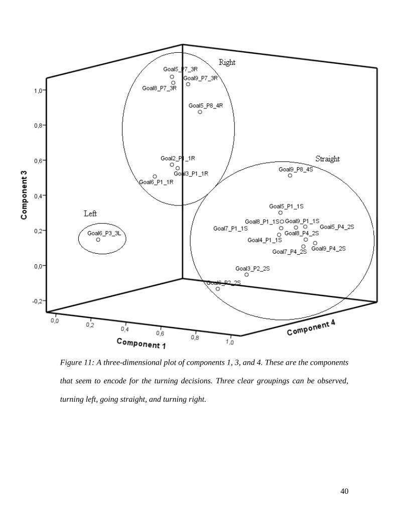
Finally, two 3D figures are shown, figure 11, and 12. Figure 11 observes all

components that encode for direction. It shows that a clear representation exists in the

network, which distinguishes between all directions (left, straight, right). Figure 12 shows

that there is a representation in the network that distinguishes all locations and their rank

in a route, effectively showing a representational map. Note here that the rank is not

something that is explicitly known in the network, it was added in the figure for

readability. However, as the network gets feedback from the environment, it does not

need to represent rank. The environment feeds the network with the actual current

location and it is, for this network at least, irrelevant whether or not this was the expected

location.

38

Figure 9: Components 1 and 4. Component 1 seems to encode for straight vs. turning; all

instances and only the instances in which going straight is required are scoring higher

than 0.6 on the scale (circle Straight). Component 4 seems to encode for going left, the

only instance in which left is required (circle Left) scores higher than all other instances.

These two components can make a distinction between all directions: Straight, right, and

left.

39

Figure 10: Components 2 and 3. Component 3 seems to encode for turning right (circles

Right P1, Right P7, and Right P8) and other directions (‘circle’ Straight). Component 2

seems to hold some location information. This is most promonently visible for position 1

(which is the first position in every route) as all instances for position 1 score above 0.6

on component 2 scale (see circles P1 and Right P1).

40

Figure 11: A three-dimensional plot of components 1, 3, and 4. These are the components

that seem to encode for the turning decisions. Three clear groupings can be observed,

turning left, going straight, and turning right.

41

Figure 12: A three-dimensional plot of components 2, 3, and 4. In this plot, the various

choice positions in the maze are circled and labeled. Note that the 'end of the line'

positions (P5, P6, and P9) are not shown since the network never makes a decision there.

Additionally, arrows show the rank order in which each position is visited during all

possible routes. Also, note that the positions with more than one possibility to turn have

these possibilities represented in different clusters in the state space (see dashed lines in

P1 and P8).

42

6. Discussion and conclusions

First, in this chapter the theoretical demands, which became apparent in the introduction

chapter, are recapitulated to discuss the success of the neural network model. Second,

some possible improvements to the current neural network model are discussed, and

some alternative neural networks are proposed. A preliminary analysis of these

alternative networks is described. Third, the embodied network and the robotic platform

used are discussed and possible improvements are mentioned. Finally, this chapter

discusses future directions for spatial artificial neural models and the current model in

particular.

6.1 Theoretic demands from psychology

The introduction summed up some demands that a spatial artificial neural network should

meet to be rooted in psychology. First, these points are repeated, and then the results of

the current network are viewed in light of these points. For the artificial neural network to

approximate how humans build and use spatial mental representations, it must:


frames;


training;



Now that the neural network model is tested, we can investigate its performance in

respect to the demands that came from the literature. First, the different spatial reference

43

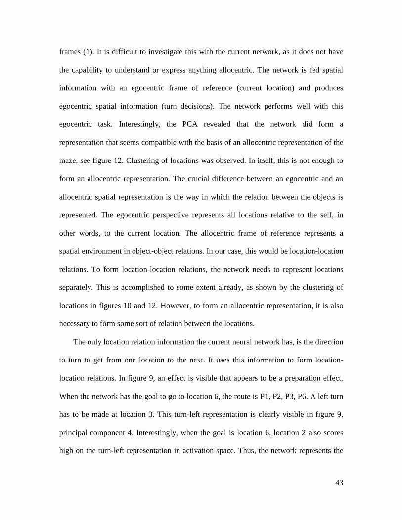
frames (1). It is difficult to investigate this with the current network, as it does not have

the capability to understand or express anything allocentric. The network is fed spatial

information with an egocentric frame of reference (current location) and produces

egocentric spatial information (turn decisions). The network performs well with this

egocentric task. Interestingly, the PCA revealed that the network did form a

representation that seems compatible with the basis of an allocentric representation of the

maze, see figure 12. Clustering of locations was observed. In itself, this is not enough to

form an allocentric representation. The crucial difference between an egocentric and an

allocentric spatial representation is the way in which the relation between the objects is

represented. The egocentric perspective represents all locations relative to the self, in

other words, to the current location. The allocentric frame of reference represents a

spatial environment in object-object relations. In our case, this would be location-location

relations. To form location-location relations, the network needs to represent locations

separately. This is accomplished to some extent already, as shown by the clustering of

locations in figures 10 and 12. However, to form an allocentric representation, it is also

necessary to form some sort of relation between the locations.

The only location relation information the current neural network has, is the direction

to turn to get from one location to the next. It uses this information to form location-

location relations. In figure 9, an effect is visible that appears to be a preparation effect.

When the network has the goal to go to location 6, the route is P1, P2, P3, P6. A left turn

has to be made at location 3. This turn-left representation is clearly visible in figure 9,

principal component 4. Interestingly, when the goal is location 6, location 2 also scores

high on the turn-left representation in activation space. Thus, the network represents the

44

relation between the two locations (P2 and P3) and their relative turning decisions. This

is a consequence of the sensitivity for sequential information of this network, as it has a

recurrent loop (Elman, 1991). It is possible to interpret this effect as a preparation effect,

a preparation or expectation to go left shortly. However, it is also possible to interpret this

as a location-location relation or an emerging allocentric representation.

Humans seem to benefit from a consistent frame of reference when learning spatial

relations (2). As of yet, this is not possible to test with the current neural network, as it

can only be fed (and thus learn) egocentric relations. Even if there is a hint at different

frames of reference in the spatial representation, the network cannot express such

knowledge. Thus, multi-frame of reference information would remain implicit.

Therefore, whether an artificial neural network would benefit from a consistent frame of

reference can only be investigated if such a network can understand and express different

frames of reference.

The use of goals in the network (3) was implemented successfully. The network

consistently reached the goal. In addition, it was tested whether an artificial neural

network could learn overlapping routes without the aid of goals. This was not possible,

without the goals, the network was not able to discern between routes. That meant that at

a choice intersection, the network „chose‟ the direction that occurred most often in the

learned set.

As mentioned earlier, the network was able to select familiar routes. In the current

experiment, the maze did not allow for the computing of novel routes (4). Each location

had a route leading to it and all these routes were taught to the network already. However,

not every route possible in the maze was taught. For example, a more efficient route to

45

location 5 would be P1, P2, P5. Not surprisingly, the network was unable to find such

alternate routes. It did not have any information to infer that this would be possible. To

make this possible, the network needs to know that P2 and P5 are adjacent.

In an informal follow up experiment, only the routes to each possible „end point‟

were taught to the network (the routes to P5, P6, and P9), see figure 4. The network was

able to get to each of these locations, following the learned route. However, the network

was not able to reach the locations in between the „end points‟. Therefore, it seems that

the network had not induced the other locations as possible goals. Concluding, it seems

unlikely an artificial neural network such as the current network, will be able to compute

novel routes.

Summarizing, of the demands that came from the psychology literature, demands 1

and 3 were implemented successfully in the current mental model. The neural network

was devised with egocentric representations in mind. It was fed only egocentric

information, yet it managed to form a representation that hinted at an emerging

allocentric representation. In addition, the use of goals was implemented successfully and

goals were found to be instrumental to distinguish between overlapping routes. Novel

route finding is not a capability of this network. Finally, the benefit of frame of reference

consistency was untestable, as the network was not able to express itself in other frames

of reference than the egocentric frame.

6.2 Theoretic demands from neurophysiology

This section discusses the specifications that a spatial artificial neural network should

meet in order to be rooted in neurobiology. First, these points are repeated and then the

46

current network is reviewed in light of these points. In order for the artificial neural

network to maintain rooted in biology, it should follow these guidelines:


(6) The model should have simple mechanisms to produce cognition;

(7) Such mechanisms should be like building blocks;



First, point (5) is not really a demand; it is more of an allowance. The network was

able to perform a route navigation task only. A next generation of this artificial neural

model should have more abilities. For example, it should have the ability to learn and

express different frames of reference. Many additions to the current network can be

envisioned, which brings us to the next neurobiological specifications.

The current neural network was constructed from several building blocks (7).

Primary building blocks are the input, output, and hidden layers, which make up many

neural networks. These building blocks are simple (6) and can be combined in many

ways (8).

The building block „input layer‟ was used twice, once as the input layer in the

traditional sense, and once as the input for context. This context allowed the network to

represent goals, which allowed for a correct distinction between overlapping routes.

Combining two hidden layers in a recurrent manner created sensitivity to the sequential

nature of routes. In literature, both recurrent networks (e.g. Elman, 1991) and context

layers (e.g. McClelland & Rogers, 2003) were used individually before. However, to the

47

best of our knowledge, no other integration of a recurrent and a contextual network exists

at this moment.

6.3 Model improvement

Clearly, there is room for improvement to the current network model. In this section,

ideas for improving the current model are discussed. As mentioned earlier, the network

was not able to infer novel routes. Informal analysis showed this is not possible with the

current neural network (see discussion of point (4) earlier). This did not come as a

surprise, because with the data the network had available, even humans would unlikely

infer novel routes. Foo et al. (2005) found that humans were able to infer novel routes

only when landmarks were available. Therefore, it seems logical that some form of

landmark recognition is needed in the artificial mental model, before novel route finding

can be expected.

The current model could only handle a situation in which the starting location was

known. From this starting position (the X in figure 4), each location taught, was

reachable. This was also true if the robot started at an intermediate location on the route,

as long as the direction the robot was facing was as prescribed by the route. If, for

example, we would put the robot in front of location 3, it would not be able to reach any

location other than location 6. Moreover, this would only work if the robot was facing in

the correct direction, between locations 2 and 3 and towards location 3 (see figure 4).

This is of course a serious limitation and should be improved in a future model.

One way to tackle the „starting anywhere‟ problem is the availability of „movement

history‟ or knowing what the previous location was. The network would have to be

48

explicitly aware of where it was before, in addition to where it is now. In this manner, it

should be possible to infer the direction of travel. Considering the maze (figure 4), for

example, if the current location is 3 and the previous location was 2, it can be inferred we

are traveling „east‟. If such a system is implemented, it is possible to find any goal

location, provided a route towards the goal was learned. The robot could wander around

randomly, until it recognizes a piece of the route (or the goal itself). Once the robot is on

the route to the goal, to reach the goal the route can be followed.

Figure 13 shows a preliminary model that might accomplish such a feat. Both current

and previous locations are presented as input, along with a goal as the context input. To

implement this idea in an embodied system, additional programming is required (e.g. the

random driving, turning around when driving into a dead end). In addition, it is not clear

what response the network should give as long as it does not „recognize‟ a route to its

goal. As such, the model shown in figure 13 is a stepping-stone towards a model that can

solve all these problems.

49

Figure 13: A preliminary neural network model that might eventually be able to start

anywhere in a maze and still get to its specified goal. Both previous and current location

are presented as input.

6.4 Embodied system

The embodiment of the neural network did not present insurmountable problems. This

does not mean there were no problems. The Lego Mindstorms platform is limited, as it is

a toy. A sophisticated toy, but a toy nonetheless. As described earlier, the color sensor

was troublesome. It produced many errors, even after precautions were taken to reduce

errors. The color sensor had to detect a color for at least 100 ms without interruption,

before the color was confirmed. In addition, the memory of the platformonly 256

50

kilobyte. This means that it is not possible to store and manipulate a large neural network.

Using the current programming code, a network of 150 neurons and 4000 links is the

approximate maximum size. Finally, using a real-time Bluetooth link between the robot

and a PC was not feasible. More information on the platform can be found in appendix C.

An additional idea for improving the (embodied) network is error checking. As

described earlier, the embodied system did not always get to its goal. The cause of such

failures was attributed to the color sensor, which was instrumental in detecting the current

location. Therefore, it seems wise to implement error checking. It might be possible to

use the neural network for this. The network can predict the next location, in addition to

the direction to turn. Following the turning direction will yield an updated 'current

location'. The (previous) prediction could be compared to this new current location. If

they do not match, something has gone wrong. Then, the robot might take action to

correct the problem, for example backtracking to the previous location or rescanning the

current location to check if it was a sensor error. In one of the earlier versions of the

network model, predicting the next location was a feature. It was scrapped because it was

deemed unnecessary for the task and tests at hand. The network model with the

prediction of the next location can be seen in figure 14.

51

Figure 14: The neural network model is capable of predicting the next location in a

route, in addition to the direction to turn in order to get there.

6.5 Practical implications and future directions

Most researchers are faced with the question „But what is the practical implication?‟ after

painstakingly elaborating on the theoretical side of their research. Therefore, a discussion

of possible practical implications for the current network and future improved versions is

given. First, the obvious practical application is embodying an artificial neural network in

some robot or device that needs to find its way. As an example, an automated vacuum

cleaning robot, such as the Roomba, might utilize a way finding neural network to find its

docking station when it needs to recharge. Alternatively, it could be taught to visit places

52

it did not visit for a long time and use the network to navigate there. Especially in

combination with the ability to learn new environments on its own, this could be a

application.

Another application lies in combining several artificial neural networks, to create

machines that can display more elaborate and complex behavior. There is a very wide

array of artificial neural networks with different functions out there. A route-finding

network like the current network, combined with a visual recognition network might

yield a system for, for example, search tasks where route information is vital. In

particular, after a disaster, it can be useful to have small robots search the rubble of a

collapsed building for survivors. It might be possible to get the robots to deliver vital

supplies, such as water, to the survivor, sustaining them while they wait for rescue

workers to reach them.

Combining of artificial neural networks is an interesting field that, in my opinion,

deserves further research. Especially, when neural networks are combined in a

hierarchical way. For example, in this thesis, the network received its input, a location,

from the program. The program read the color sensor and stored all the colors of the color

code. Then it looked up the code in a library and fed the corresponding location as input

to the network. It is also possible to let a neural network do this. It seems trivial to use a

neural network for a task such as looking up a color code, nevertheless, a more complex

visual system could benefit from the associative powers of a neural network. Such a

system could first recognize a visual scene and then stimulate the representation of this

scene in a route-finding network. A similar hierarchic structure can be envisioned for the

motor system. The embodied system in the current thesis already used a neural network

53

to avoid collisions. This lane-keeping network was completely independent from the

route-finding network, however.

There seems to be sense in thinking that combining more networks might be

beneficial. Especially in an application with limited sensors such as the Lego Mindstorms

robot, using all available sensor data seems wise. One network, for example the route

finding network, might be able to use characteristics from another network, for example

the characteristics of the lane (e.g. width), to infer more about the environment. This has

some similarities to the micro behavior approach by Ballard and Sprague (2006). Human

behavior seems to come from a collection of micro behaviors. Simple neural networks

can produce such micro behaviors. A neural network consisting of several simple but

closely interconnected networks might reveal 'larger' (macro) behaviors. In addition,

combining several neural networks seems to be in accordance with neurobiology as the

(human) brain consists of many closely interconnected networks. Combinations of

closely interconnected simple neural networks might reveal interesting and novel

solutions to a problem or a task.

54

References

Ballard, D., & Sprague, N. (2006). Modeling the brain‟s operating system using virtual

humanoids. International Journal of Pattern Recognition and Artificial Intelligence,

20 (6), 797-815.

Bechtel, W., & Abrahamsen, A. (2001). Connectionism and the mind: an introduction to

parallel processing in networks. Blackwell Publishers.

BricxCC. (2011). Version 3.3.8.10, downloaded March 2011 via

http://bricxcc.sourceforge.net.

Brunyé, T.T., Rapp, D.N., & Taylor, H.A. (2008). Representation flexibility and

specificity following spatial descriptions of real-world environments. Cognition, 108,

418-443.

Burgess, N. (2006). Spatial memory: how egocentric and allocentric combine. Trends in

Cognitive Sciences, 10 (12), -551-557.

Burgess, N., Becker, S., King, J.A., & O‟Keefe, J. (2001). Memory for events and their

spatial context: models and experiments. Philosophical Transactions of the Royal

Society B: Biological Sciences, 356 (1413), 1493-1503.

Cocude, M., Mellet, E., & Denis, M. (1999). Visual and mental exploration of visuo-

spatial configurations: Behavioral and neuroimaging approaches. Psychological

Research, 62, 93–106.

Denis, M., & Zimmer, H.D. (1992). Analog properties of cognitive maps constructed

from verbal descriptions. Psychological Research, 54, 286-298.

Desouza, G.N.; Kak, A.C. (2002). Vision for mobile robot navigation: a survey. Pattern

Analysis and Machine Intelligence, IEEE Transactions, 24 (2), 237-267.

55

Egmont-Petersen, M., de Ridder, D., & Handels, H. (2001). Image processing with neural

networks--a review, Pattern Recognition, 35 (10), 2279-2301.

Elman, J.L. (1991). Distributed representations, simple recurrent networks, and

grammatical structure. Machine Learning, 7, 195-225.

Erlhagen, W., Bastian, A., Jancke, D., Riehle, A., & Schöner, G. (1999). The distribution

of neuronal population activation (DPA) as a tool to study interaction and integration

in cortical representations. Journal of Neuroscience Methods, 94, 53-66.

Foo, P., Warren, W.H., Duchon, A., & Tarr, M.J. (2005). Do humans integrate routes into

a cognitive map? Map- versus landmark-based navigation of novel shortcuts. Journal

of Experimental Psychology: Learning, Memory, and Cognition, 31 (2), 195-215.

Ghaem, O., Mellet, E., Crivello, F., Tzourio, N., Mazoyer, B., Berthoz, A., & Denis, M.

(1997). Mental navigation along memorized routes activates the hippocampus,

precuneus, and insula. NeuroReport, 8, 739-744.

Grossberg, S. (1980). Biological competition: Decision rules, pattern formation, and

oscillations. Proceedings of the National Academy of Sciences (USA), 77, 2338-2342.

Hecht-Nielsen, R. (1989). Theory of the backpropagation neural network. Neural

Networks, 1989. IJCNN., International Joint Conference, 1, 593-605.

HiTechnic. (2011). NXT Color Sensor Version 2 for LEGO MINDSTORMS NXT,

downloaded June 2011 via:

http://www.hitechnic.com/cgi-bin/commerce.cgi?preadd=action&key=NCO1038

Hothersall, D. (2004). History of Psychology, Mc Graw Hill Companies, New York.

Kutner, M.H., Nachtsheim, C.J., Neter, J, & Li, W. (2005). Applied Linear Statistical

Models. Mc Graw Hill, New York.

56

Lipinski, J., Sandamirskaya, Y., & Schöner, G. (2009). Swing it to the Left, Swing it to

the Right: Enacting Flexible Spatial Language Using a Neurodynamic Framework.

Cognitive Neurodynamics 3(4), 1-39.

Maguire, E.A., Gadian, D.G., Johnsrude, I.S., Good, C.D., Ashburner, J., Frackowiak,

R.S.J., & Frith, C.D. (2000). Navigation-related structural change in the hippocampi

of taxi drivers. PNAS, 97 (8), 4398-4403.

Mayerich, D., Abbott, L., & McCormick, B. (2008). Knife-edge scanning microscopy for

imaging and reconstruction of three-dimensional anatomical structures of the mouse

brain. Journal of Microscopy, 231, 134-143.

Mellet, E., Bricogne, S., Tzourio-Mazoyer, N., Ghaëm, O., Petit, L., Zago, L., Etard, O.,

Berthoz, A., Ma-zoyer, B., & Denis, M. (2000). Neural Correlates of Topographic

Mental Exploration: The Impact of Route versus Survey Perspective Learning.

NeuroImage, 12, 588-200.

MemBrain. (2010). Version 03.06.02.00, downloaded January 2011 via www.membrain-

nn.de.

Noordzij, M. L., & Postma, A. (2005). Categorical and metric distance information in

mental representations derived from route and survey descriptions. Psychological

Research, 69, 221-232.

Noordzij, M.L., Zuidhoek, S., & Postma, A. (2006). The influence of visual experience

on the ability to form spatial mental models based on route and survey descriptions.

Cognition, 100, 321-342.

Pomerleau, D.A. (1989). ALVINN: An autonomous land vehicle in a neural network

Technical Report CMUCS-89-107. Carnegie Mellon University.

http://www.membrain-nn.de/

http://www.membrain-nn.de/

57

Rogers, T.T., & McClelland, J.L. (2008). Précis of Semantic Cognition: A Parallel

Distributed Processing Approach. Behavioral and Brain Sciences, 31, 689-714.

Ruini, F., Cangelosi, A., & Zetule, F. (2009). Individual and cooperative tasks performed

by autonomous MAV teams driven by embodied neural network controllers.

Proceedings of international joint conference on neural networks.

Schöner, G. (2006). Dynamical systems approaches toward cognition. In R.Sun (Ed.),

Cambridge handbook of computational psychology (pp. 101–126). New York:

Cambridge University Press. Downloaded from: http://fog.its.uiowa.edu/~icdls/dft-

school/documents/DFT_Publications/cambridge_chapter_schoner.pdf

Taylor, H.A., Brunyé, T.T., & Taylor, S.T. (2008). Spatial Mental Representation:

Implications for Navigation System Design. Reviews of Human Factors and

Ergonomics, 4, 1-40.

Toledo, S. (2006). Analysis of the NXT Bluetooth-Communication Protocol. Retrieved

February 10, 2011, from http://www.tau.ac.il/~stoledo/lego/btperformance.html

van Gelder, T., & Port, R.F. (1995). It‟s about time: An overview of the dynamical

approach to cognition. In: Mind as motion, ed. R. F. Port & T. van Gelder, 1-44. MIT

Press.

van der Velde. F. (2010). Where Artificial Intelligence and Neuroscience Meet: The

Search for Grounded Architectures of Cognition. Advances in Artificial Intelligence,

2010, 1-18.

Waller, D., & Hodgson, E. (2006). Transient and Enduring Spatial Representations Under

Disorientation and Self-Rotation. Journal of Experimental Psychology: Learning,

Memory, and Cognition, 32 (4), 867-882.

58

Wang, R.F., & Spelke, E.S. (2000). Updating egocentric representations in human

navigation. Cognition, 77, 215-250.

Wang, R.F., & Spelke, E.S. (2002). Human spatial representation: insights from animals.

Trends in Cognitive Sciences, 6 (9), 376-382.

Zaehle, T., Jordan, K., Wüstenberg, T., Baudewig, J., Dechent, P., & Mast, F.W. (2007).

The neural basis of the egocentric and allocentric spatial frame of reference. Brain

Research, 1137, 92-103.

Zeidenberg, M. (1990). Neural Networks in Artificial Intelligence. Ellis Horwood, New

York.

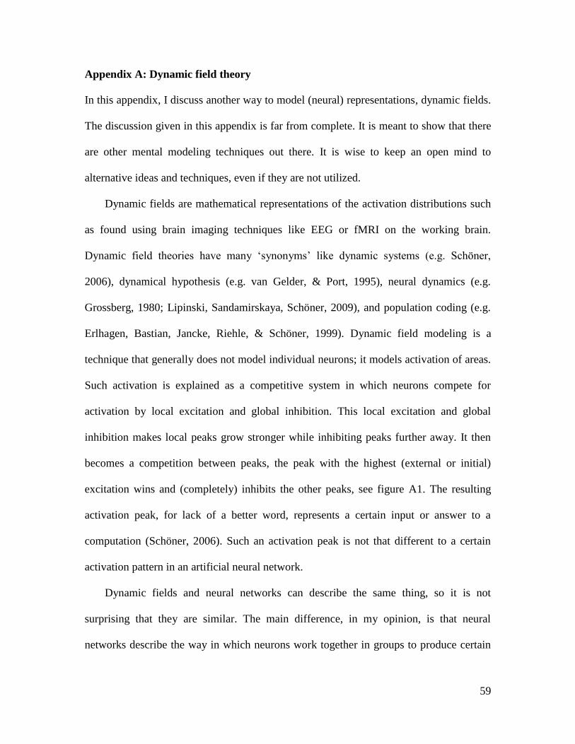
59

Appendix A: Dynamic field theory

In this appendix, I discuss another way to model (neural) representations, dynamic fields.

The discussion given in this appendix is far from complete. It is meant to show that there

are other mental modeling techniques out there. It is wise to keep an open mind to

alternative ideas and techniques, even if they are not utilized.

Dynamic fields are mathematical representations of the activation distributions such

as found using brain imaging techniques like EEG or fMRI on the working brain.

Dynamic field theories have many „synonyms‟ like dynamic systems (e.g. Schöner,

2006), dynamical hypothesis (e.g. van Gelder, & Port, 1995), neural dynamics (e.g.

Grossberg, 1980; Lipinski, Sandamirskaya, Schöner, 2009), and population coding (e.g.

Erlhagen, Bastian, Jancke, Riehle, & Schöner, 1999). Dynamic field modeling is a

technique that generally does not model individual neurons; it models activation of areas.

Such activation is explained as a competitive system in which neurons compete for

activation by local excitation and global inhibition. This local excitation and global

inhibition makes local peaks grow stronger while inhibiting peaks further away. It then

becomes a competition between peaks, the peak with the highest (external or initial)

excitation wins and (completely) inhibits the other peaks, see figure A1. The resulting

activation peak, for lack of a better word, represents a certain input or answer to a

computation (Schöner, 2006). Such an activation peak is not that different to a certain

activation pattern in an artificial neural network.

Dynamic fields and neural networks can describe the same thing, so it is not

surprising that they are similar. The main difference, in my opinion, is that neural

networks describe the way in which neurons work together in groups to produce certain

60

activations and that the dynamical fields describe the overall distribution of activation.

Another way of putting it, dynamic fields use an „infinite‟ number of neurons to plot an

activation pattern, while neural networks use a finite number.

Figure A1: Local excitatory interaction helps sustain localized peaks of activation while

long-range inhibitory interaction prevents diffusion of peaks and stabilizes against

competing inputs (from Schöner, 2006).

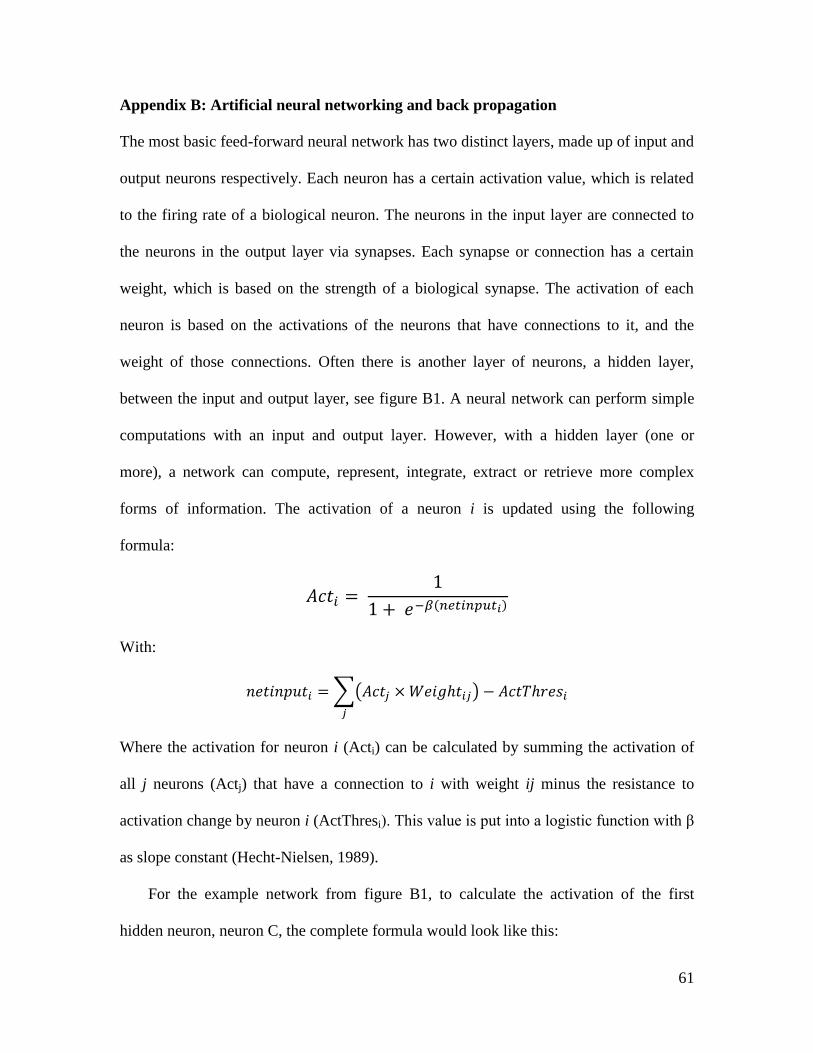
61

Appendix B: Artificial neural networking and back propagation

The most basic feed-forward neural network has two distinct layers, made up of input and

output neurons respectively. Each neuron has a certain activation value, which is related

to the firing rate of a biological neuron. The neurons in the input layer are connected to

the neurons in the output layer via synapses. Each synapse or connection has a certain

weight, which is based on the strength of a biological synapse. The activation of each

neuron is based on the activations of the neurons that have connections to it, and the

weight of those connections. Often there is another layer of neurons, a hidden layer,

between the input and output layer, see figure B1. A neural network can perform simple

computations with an input and output layer. However, with a hidden layer (one or

more), a network can compute, represent, integrate, extract or retrieve more complex

forms of information. The activation of a neuron i is updated using the following

formula:

With:

Where the activation for neuron i (Acti) can be calculated by summing the activation of

all j neurons (Actj) that have a connection to i with weight ij minus the resistance to

activation change by neuron i (ActThresi). This value is put into a logistic function with β

as slope constant (Hecht-Nielsen, 1989).

For the example network from figure B1, to calculate the activation of the first

hidden neuron, neuron C, the complete formula would look like this:

62

Figure B1: A simple feed forward network. Two input neurons in the input layer at the

top, feed into two hidden neurons in the hidden layer, which feed into the single output

neuron in the output layer at the bottom.

The way in which the neurons are interconnected and also the weight of these

connections can be hardwired into the network by a network designer. Most feed-forward

neural networks, however, employ a learning mechanism. Back propagation is a method

in which the error, the difference between the current output and the desired output, of a

63

neural network is reduced by altering the weight of the (synaptic) connections between

the neurons of the network (Hecht-Nielsen, 1989).

Often, learning starts with a randomization of all the weights. This insures that all

connections have a value, which can be of importance in some programming languages.

Next, each item in a training set is presented to the network. When the input layer of the

network is stimulated in accordance with an item, the network calculates the activation of

each neuron (using the formula described above). This feed forward phase will generate

an activation for the output neurons that is likely incorrect. Thus, for every output neuron

(u) there is a difference between desired output activation (du) and actual output

activation (au). The error of the entire network is calculated as follows:

When the error of network is found, the relative culprits to the error have to be

found. In other words, the portion that each neuron contributes to the error has to be

calculated in order to change the weight of the connection between the two neurons

involved. The portion of error fed to the output neurons came from the hidden layer (one

layer up). Therefore, the weight change necessary for all weights has to be calculated:

and

thus,

64

where

Now the input is traced back to the neuron in the layer above, in this case the hidden

layer (h). First, calculate the portion of activation this weight contributed:

So, now finally it is possible to calculate the portion of error this weight contributed:

Now change of weight can be calculated using the Hebbian learning rule:

Where, lrate is the learning rate. Thus, the weight change is calculated:

Weight changes deeper in the network are calculated iteratively. This means that the

delta for the hidden layer (deltah) nests the delta for the output layer (deltau):

For the three-layered network, as displayed in figure B1, the final weight change is

calculated as follows:

For more information, refer to Bechtel and Abrahamsen (2001).

65

Appendix C: Guidance

In this appendix, four guides are included. The programs used to create the neural

network for this thesis are discussed first. Next, the code is discussed and it is explained

how to update the current code with another neural net. For example, if a new spatial

environment is learned. Next, the platform used to embody the neural network is

discussed. Special focus is on the limitations of the platform. Finally, a building guide is

included to recreate Wobot, the robot used in this thesis.

Guide to MemBrain

Modeling an artificial neural network with many neurons is not easy, especially if you

want to test many different versions of a neural network model. Fortunately, there are off-

the-shelf tools available that can assist in such a task. MemBrain Neural Network

Simulator, version 03.06.02.00, is such a tool. It allows users to model, teach, test, and

export neural networks of arbitrary size and architecture (MemBrain, 2011).

MemBrain offers sufficient tutorials for novices to become acquainted with the

program and its capabilities. Therefore, I will not describe how to create or teach a neural

network. In order to use the trained neural network, it has to be exported. MemBrain can

export a network in C code. Via the menu bar, code can be generated, see figure C1.

Figure C1: A screenshot of the code-generation menu in MemBrain.

66

Figure C2: A very simple neural network in MemBrain. At the top, an input neuron

(named 1) with activation 1 is visible. In the middle, the hidden neurons (2 and 3) are

shown. At the bottom, output neuron (4) is visible. The weights are visible as the numbers

on the lines between the neurons. The activation of the neurons is visible beneath the

neuron.

The generated code for a very simple network, see figure C2, is located in a file

named NeuralNetDef.c. Not shown in the figure are the activation thresholds of the

hidden neurons, which are 0.22 for neuron 2 and 0.33 for neuron 3. The values of interest

in this file look like this:

// additional parameters for all hidden neurons

const SHiddenNeuronParms NEURON_PARMS_HIDDEN[] =

{

(FLOAT32)0.22, 0, 1,

(FLOAT32)0.33, 1, 1

};

/// additional parameters for all output neurons

const SOutputNeuronParms NEURON_PARMS_OUTPUT[] =

{

(FLOAT32)0, 2, 2

};

67

/// parameters for all links

const SNeuralLinkParms NEURAL_LINK_PARMS[] =

{

(FLOAT32)0.12, 0,

(FLOAT32)0.13, 0,

(FLOAT32)0.24, 1,

(FLOAT32)0.34, 2

};

For the NXC compiler to understand this code, some modifications are needed. Refer

to appendix F for the proper syntax. The parameters for the hidden neurons consist of

three values; the activation threshold, and two values that are used in looking up the

weights for the incoming links to this neuron. For example for neuron 2: we know it has

an activation threshold of 0.22. We can look this up in the array and notice neuron two is

described in the first line (i.e. 0.22, 0, 1). The first number is the activation threshold. The

second number is the location of the first link in the array with link information

(NEURAL_LINK_PARMS). The third number (1) is the amount of input links, and thus

the amount of lines in the link-array that have to be read. Observing the first line in the

NEURAL_LINK_PARMS array confirms this is correct. We can observe the correct

weight (0.12) for the link to neuron 2. In addition, in this line we observe another

number. This number corresponds to an input neuron. In our case this is 0, as the input

neuron is the first neuron (and in computer languages it is common to start counting at 0).

To confirm this, we can look at the second line in the links-array and see that the second

number is also a 0, which is fortunate because the weight 0.13 corresponds to the other

link to the input neuron.

I am aware that the above does not seem very intuitive, but it is how the neural

modeling tool MemBrain exports its neural networks (apparently, nothing is easy). It took

68

some effort on my part to comprehend this exported code, but with the above (and

perhaps some trial-and-error); it should possible for others to understand it readily.

Guide to code changes in BricxCC

The Lego Mindstorms brick can be programmed in Not eXactly C (NXC), which is a

high-level language similar to C. NXC code can be compiled and uploaded to the brick

using, BricxCC (BricxCC, 2011). For this thesis, the code was divided in two files; the

algorithms (see appendix E) and the variables (see appendix F). The code in appendix E

includes the 'task main', which starts all other tasks and sub routines. The code in

appendix F is included at the top of the code in appendix E, effectively telling the

compiler to start the byte-code with F and follow with E.

In most cases, changes in the code are done in appendix F only. For example, if the

network learned new routes, the new exported network should replace the current

network in the code. In addition, if the network layout has changed, values for the

network layout in appendix F may have to be updated.

In some cases, adaptations need to be made to the program itself. To understand the

program, a flowchart is included (see figure C3). When the program begins, first the user

has to select a goal via the task 'goal button'. Then, the control task is started. This task

keeps track of the sensors. The control task makes decisions based on the sensor data, and

in particular, the color sensor. As long as the control task does not detect a color code, the

lane-keeping task is activated. This task moves the robot forward and steers it clear of

obstacles. When a color code is detected, the code is translated into a location. If this

location is the destination, the program ends. If the location is not the destination, it is fed

69

to the navigation. This navigation task holds the artificial neural network. The network

generates a turning decision (left, right or straight). A left or right turn cannot be executed

by the lane-keeping task, and thus a separate task turns the robot in the desired direction.

If the turn is completed, or no turn was required, the control task restarts the lane-keeping

task. This moves the robot forward, until another (new) location is found.

Guide to Lego Mindstorms

The Lego Mindstorms platform is a very sophisticated toy, but a toy nonetheless. Maybe

as such, it has its limitations, most notably for this thesis, the color sensor. It was not very

reliable and extremely sensitive to the distance to the object. As described in the thesis,

the sensor had problems with determining the correct color (e.g., the sensor found pink

more red that actual red). Also, the sensor would only operate correctly if it was exactly 2

mm above the colored surface. Any bump in the surface or vibrations as the robot drove

along caused the distance between sensor and surface to change. This meant the sensor

registered black or more sporadically a different, unpredictable color. Often, this made

the robot unable to reach its destination. It got lost.

A solution might be available. A different color sensor for the Lego Mindstorms

platform is on the market; the HiTechnic NXT Color Sensor Version 2 for LEGO

MINDSTORMS NXT (HiTechnic, 2011). This sensor can detect more colors (18 instead

of 6) and it is less sensitive to surface-sensor distance, see figure C4.

70

Figure C3: The flowchart for the Wobot software. The squares represent tasks and the

diamonds represent decision points.

71

The Lego Mindstorms brick features a very limited amount of memory and little

processing power. It has a 16 MHz processor and only 256 kilobytes of memory (shared

storage and working memory). The processing and memory limits led to a pursuit of a

setup in which the neural network could be run externally (on a PC). This would

circumvent the limits of the brick and allow for online learning of the neural network.

A real-time Bluetooth connection to a PC was considered. It was investigated

whether the robot could send real-time sensor data to a PC, which would send back motor

commands. The way the Bluetooth is setup in the Mindstorms platform, would mean a

minimum delay of 100-200 ms between when sensor data was send and when motor

commands could be received. The Bluetooth radio in the brick would be solely

responsible for this delay (Toledo, 2006). Other possible delays would add up, such as

the processing of commands in the brick or learning of the neural network on the remote

PC. Such delay seemed impractical in the navigation task (and the obstacle avoidance)

and a locally run artificial neural network approach was pursued. This approach has an

advantage. The neural network is 'really' embodied and not embodied but run externally.

72

Figure C4: The HiTechnic NXT Color Sensor Version 2 for LEGO MINDSTORMS NXT

in a setup that shows its optimal positioning (HiTechnic, 2011).

Building guide to Wobot

I created a Lego building guide for the robot. The guide is not included here, as it is

rather voluminous. It is available on Google Docs, via:

https://docs.google.com/viewer?a=v&pid=explorer&chrome=true&srcid=0B4oq088EBZ

YeZjVhYTA4YzQtNTFkMi00OGI3LThjZDMtMDA1NTkxOTNjMTAw&hl=en_US

https://docs.google.com/viewer?a=v&pid=explorer&chrome=true&srcid=0B4oq088EBZYeZjVhYTA4YzQtNTFkMi00OGI3LThjZDMtMDA1NTkxOTNjMTAw&hl=en_US

https://docs.google.com/viewer?a=v&pid=explorer&chrome=true&srcid=0B4oq088EBZYeZjVhYTA4YzQtNTFkMi00OGI3LThjZDMtMDA1NTkxOTNjMTAw&hl=en_US

73

Appendix D: Neural network in MemBrain

In this appendix, the route finding network as modeled using MemBrain (2011) is

displayed. This neural network learned a set of routes and the necessary turning decisions

at the various locations along each route. In the figure location 9 is the goal and the

current location is 8, resulting in the output 'straight'. See figure D1 caption for more

details on the network layout.

Figure D1: The route finding neural network as modeled in MemBrain. At the top the

three input groups are visible. The top left shows a group of hidden neurons that are a

copy of the previous activation in the first hidden layer. The top middle group of neurons

inputs the current location to the network. At the top right, the neurons that encode for

the goal location of a route are visible. At the bottom the output layer is visible,

consisting of three neurons for the three possible turns. Between the input and output

layers, the two hidden layers can be observed. (Image adapted from Membrain Neural

Network Simulator).

74

Appendix E: NXC code, algorithms

The code used to embody the artificial neural network in the Lego Mindstorms robot is

displayed in this and the next appendix. The code is organized in two appendices,

because a differentiation was made between algorithms and variables. This appendix (E)

contains all algorithms and the next appendix (F) contains all variables, including the

variables for the neural networks. This means that someone who wants to change the

weights of the neural network described in this thesis or the amount of neurons in the

network, only makes changes to appendix F. If you wish to implement a different

network, changes to the code described in this appendix might be necessary.

The code is written in Not eXactly C (NXC), which is a high-level language similar

to C. It can be used to program the Lego Mindstorms NXT brick. NXC programs can be

compiled and uploaded to the Lego Mindstorms brick using Bricx Command Center

(BricxCC, 2011).

#include "include.nxc"

//using buttons to select goal, returns goal

sub goalbutton()

{

TextOut(0, LCD_LINE1, "Select goal and");

TextOut(0, LCD_LINE2, "press start:");

goal = 1;//start at

while ( ButtonPressed(BTNCENTER, true) != true ) //wait for start

{

ClearLine(LCD_LINE4);

NumOut(0,LCD_LINE4, goal);

if ( ButtonPressed(BTNRIGHT, true) != false) //press right is +1

{

if (goal < aant_locations) //highest goal is number of locations in maze

{goal++;

Wait(300);}

else

}

75

else if ( ButtonPressed(BTNLEFT, true) != false) //left is -1

{

if (goal > 1) //lowest goal is 1

{goal--;

Wait(300);}

else

}

else

}

ClearScreen();

TextOut(0,LCD_LINE1, "Ok, going to");

NumOut(0,LCD_LINE2, goal);

Wait(1000);

ClearScreen();

} //end goalbutton

//sensor can be called to renew sensordata (distance)

sub sensor()

{

//what sensor on what port

SetSensorLowspeed(IN_1);



//reading sensor values

DistMid = SensorUS(IN_1);

DistRight = SensorUS(IN_2);

DistLeft = SensorUS(IN_3);

} //end sensor

//sensorcolor can be called to update sensordata (color)

sub sensorColor() //extra steps because of noisy color sensor data

{

SetSensorColorFull(IN_4);

int sensorraw;

int ik =0;

while (true) //executes till new color is confirmed

{

sensorraw = Sensor(IN_4);

Wait(1);

if (sensorraw == Sensor(IN_4)) //true if after 1ms color is the same

{

ik++;

}

if (sensorraw != Sensor(IN_4)) //reset counter if color changed

{

76

ik=0;

}

if (ik > kleurnauwkeurigheid) //if color is the same for long enough (kleurnauwkeurigheid), Color is updated

{

Color = sensorraw; //update Color

ik=0;

NumOut(0, LCD_LINE8, Color);

return; //stops sensorcolor

}

}//einde while

/* color sensor color codes:

1 = black

2 = blue

3 = green

4 = yellow

5 = red

6 = white

*/

}//end sensorColor

//starting color shouldnt be black, sensor might be to close to ground

sub startcheck()

{

sensorColor();

while (Color == 1)

{

TextOut(0, LCD_LINE1, "Check colorsensor");

TextOut(0, LCD_LINE2, "Color =");

NumOut(50, LCD_LINE2, Color);

sensorColor();

}

} //end startcheck

//motorpwr can be called to change motorspeeds (by lane)

sub motorpwr(int C, int B)

{

OnFwd(OUT_B, B);

OnFwd(OUT_C, C);

}

//turning on an intersection is done by this quick and dirty function, takes direction and turns robot this way

sub turn(int direction)

{


TextOut(0, LCD_LINE1, "Turn");

//little forward

OnFwd(OUT_BC, turn_straight);

Wait(1500);

77

//turn

if (direction == 0) //left

{

TextOut(60, LCD_LINE1, "Left");

OnFwd(OUT_B, turn_circle);

OnRev(OUT_C, turn_circle);

}

if (direction == 1) //straight

{

TextOut(60, LCD_LINE1, "Straight");

OnFwd(OUT_B, turn_circle);

OnFwd(OUT_C, turn_circle);

}

if (direction == 2) //right

{

TextOut(60, LCD_LINE1, "Right");

OnRev(OUT_B, turn_circle);

OnFwd(OUT_C, turn_circle);

}

Wait(600);

Coast(OUT_BC); //stop motors

op_kruising = false;


} //end turn

//task for lanekeeping, using a neural network

task lane()

{

while (currentlocation != goal) //dont drive away when you are at your destination

{

while (op_kruising == false) //dont do lanekeeping when youre on an intersection

{

sensor(); //reading (distance)sensor

//calculate input neuron activations

//input neuron[0] represents distleft, [1] = right distance, [2] = forward distance

//normalise distances to range 0 - 1, range neurons

if ((DistLeft / DistMax) < 1){

LANE_NEURON_ACT[0] = (DistLeft / DistMax);}

else {

LANE_NEURON_ACT[0] = 1; }

if ((DistMid / DistMax) < 1){

LANE_NEURON_ACT[2] = (DistMid / DistMax);}

else {

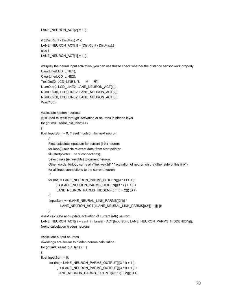
78


if ((DistRight / DistMax) <1){

LANE_NEURON_ACT[1] = (DistRight / DistMax);}

else {


//display the neural input activation, you can use this to check whether the distance sensor work properly



TextOut(0, LCD_LINE1, "L M R");

NumOut(0, LCD_LINE2, LANE_NEURON_ACT[1]);



Wait(100);

//calculate hidden neurons

//i is used to 'walk through' activation of neurons in hidden layer

for (int i=0; i<aant_hid_lane;i++)

{

float InputSum = 0; //reset inputsum for next neuron

/*

First, calculate inputsum for current (i-th) neuron:

for-loop(j) selects relevant data: from start pointer

till (startpointer + nr of connections).

Select links (ie. weights) to current neuron.

Other words, forloop sums all ("link weight" * "activation of neuron on the other side of this link")

for all input connections to the current neuron

*/

for (int j = LANE_NEURON_PARMS_HIDDEN[((3 * i ) + 1)];

j < (LANE_NEURON_PARMS_HIDDEN[((3 * i ) + 1)] +

LANE_NEURON_PARMS_HIDDEN[((3 * i ) + 2)]) ;j++)

{

InputSum += (LANE_NEURAL_LINK_PARMS[(2*j)] *

LANE_NEURON_ACT[ (LANE_NEURAL_LINK_PARMS[((2*j)+1)]) ]);

}

//next calculate and update activation of current (i-th) neuron:

LANE_NEURON_ACT[( i + aant_in_lane)] = ACT(InputSum, LANE_NEURON_PARMS_HIDDEN[(3*i)]);

}//end calculation hidden neurons

//calculate output neurons

//workings are similar to hidden neuron calculation

for (int i=0;i<aant_out_lane;i++)

{

float InputSum = 0;

for (int j= LANE_NEURON_PARMS_OUTPUT[((3 * i) + 1)];

j < (LANE_NEURON_PARMS_OUTPUT[((3 * i) + 1)] +

LANE_NEURON_PARMS_OUTPUT[((3 * i) + 2)]); j++)

79

{

InputSum += (LANE_NEURAL_LINK_PARMS[(2*j)] *

LANE_NEURON_ACT[ (LANE_NEURAL_LINK_PARMS[((2*j) + 1)]) ]);

}

//calculate activation of neuron and normalize

if (normalize == 1)

{

LANE_NEURON_ACT[(i+ aant_in_lane + aant_hid_lane)] = ((

(ACT(InputSum,LANE_NEURON_PARMS_OUTPUT[(3*i)])) *2)-1);

} else if (normalize == 0)

{

LANE_NEURON_ACT[(i+ aant_in_lane + aant_hid_lane)] =

(ACT(InputSum,LANE_NEURON_PARMS_OUTPUT[(3*i)]));

}

}//end output calculation

//motor power * activation motorneurons

motorpwr((Pwr * LANE_NEURON_ACT[7]), (Pwr * LANE_NEURON_ACT[8]));

//reset neurons for next iteration, not necessary for well trained networks

for (int c=0;c<aant_neur_lane;c++)

{

LANE_NEURON_ACT[c] = 0;

}

}//end while loop for lane keeping

}//end while current location != goal

}//end task lane

sub kruising() //kruising is Dutch for intersection

{

for (int i = 0; i<aant_iteraties; i++)

{

//input has range of 0 to 1

//input neurons

/*

Input neurons for my network are supposed to go from NAV_NEURON_ACT[0]

till NAV_NEUR_ACT[20], this means that:

vorige turns:

[0] = links

[1] = rechtdoor

[2] = right

currentlocations:

80

[3-11] are locations 1-9

goals

[12-20] are goals 1-9

*/

//first input reset to 0

for (int j=0; j<aant_in_nav;j++)

{NAV_NEURON_ACT[j] = 0;}

//then vorige turn activeren

if (direction != 99) //deze if zet alleen vorige turn aan als ie niet net geinitialiseerd is, en er dus daadwerkelijk

een vorige turn is

{NAV_NEURON_ACT[direction] = 1;}

//dan current location

NAV_NEURON_ACT[(currentlocation + 2)] = 1;

//dan goal

NAV_NEURON_ACT[(goal + 11)] = 1;

//hidden berekenen, i loopt van begin tot eind aantal hidden neuronen

//i wordt gebruikt om activatie van neuronen door te stappen

for (int i=0; i<aant_hid_nav;i++)

{

//reset voor volgend neuron

float InputSumN = 0;

/*

Eerst inputsom betreffende neuron berekenen:

for-loop(j) selecteert relevante data: van begin pointer

tot (beginpointer + aantal).

Linkjes (ie. weights) naar het betreffende neuron selecteren

*/

for (int j = NAV_NEURON_PARMS_HIDDEN[((3 * i ) + 1)];

j < (NAV_NEURON_PARMS_HIDDEN[((3 * i ) + 1)] +

NAV_NEURON_PARMS_HIDDEN[((3 * i ) + 2)]) ;j++)

{

InputSumN += (NAV_NEURAL_LINK_PARMS[(2*j)] *

NAV_NEURON_ACT[ (NAV_NEURAL_LINK_PARMS[((2*j)+1)]) ]);

}

//dan activatie van betreffende neuron berekenen:

NAV_NEURON_ACT[( i + aant_in_nav)] = ACTN(InputSumN, NAV_NEURON_PARMS_HIDDEN[(3*i)]);

}//einde hidden berekenen

//outneuronen berekenen

for (int i=0;i<aant_out_nav;i++)

81

{

//reset voor volgend neuron

float InputSumN = 0;

for (int j= NAV_NEURON_PARMS_OUTPUT[((3 * i) + 1)];

j < (NAV_NEURON_PARMS_OUTPUT[((3 * i) + 1)] +

NAV_NEURON_PARMS_OUTPUT[((3 * i) + 2)]); j++)

{

InputSumN += (NAV_NEURAL_LINK_PARMS[(2*j)] *

NAV_NEURON_ACT[ (NAV_NEURAL_LINK_PARMS[((2*j) + 1)]) ]);

}

NAV_NEURON_ACT[(i+ aant_in_nav + aant_hid_nav)] =

(ACTN(InputSumN,NAV_NEURON_PARMS_OUTPUT[(3*i)])) ;

}//einde output berekenen

//welke output hett grootst (winner takes all) is berekenen, output consequentie

if ( (NAV_NEURON_ACT[(aant_in_nav + aant_hid_nav)] > NAV_NEURON_ACT[(aant_in_nav + aant_hid_nav

+ 1)]) && (NAV_NEURON_ACT[(aant_in_nav + aant_hid_nav)] > NAV_NEURON_ACT[(aant_in_nav +

aant_hid_nav + 2)]) )

{ direction = 0; }

if ( (NAV_NEURON_ACT[(aant_in_nav + aant_hid_nav +1)] > NAV_NEURON_ACT[(aant_in_nav +

aant_hid_nav)]) && (NAV_NEURON_ACT[(aant_in_nav + aant_hid_nav +1)] >

NAV_NEURON_ACT[(aant_in_nav + aant_hid_nav + 2)]) )

{ direction = 1; }

if ( (NAV_NEURON_ACT[(aant_in_nav + aant_hid_nav +2)] > NAV_NEURON_ACT[(aant_in_nav +

aant_hid_nav)]) && (NAV_NEURON_ACT[(aant_in_nav + aant_hid_nav +2)] >

NAV_NEURON_ACT[(aant_in_nav + aant_hid_nav + 1)]) )

{ direction = 2; }

//output betekend:

//direction: left = 0, straight = 1, right = 2

}//einde forloop

//output geven aan turn

turn(direction);


NumOut(0, LCD_LINE7, direction);

TextOut(10, LCD_LINE7, "direction");

Wait(2000);

//neuronen resetten voor volgende iteratie

/*for (int a=0;a<aant_neur_nav;a++)

{

NAV_NEURON_ACT[a] = 0;

} */

} //einde navigatie

sub code() //hij komt hier binnen als ie van wit af is

82

{

int j = 0;

int temp = 0;

while (Color != 6) //zolang niet op wit (=kruispunt) kleur opslaan

{

/* if ((j == 0) && (Color != 0) && (Color !=6) && (Color !=1) && (aant_strepen_kleurcode > j)) //eerste kleur

opslaan

{

CurrentCode[j] = Color;

j++;

} */

sensorColor(); //volgende kleur halen

if ((Color != temp) && (Color != 0) && (Color !=6) && (Color !=1) && (aant_strepen_kleurcode > j)) //true als

nieuwe kleur, niet lege waarde en niet zwart of wit

{

CurrentCode[j] = Color;

temp = Color;

j++;


NumOut(0, LCD_LINE5, j);

TextOut(10, LCD_LINE5, "Colors counted");

}

/*if (aant_strepen_kleurcode < j)

{

return; //uit while stappen

} */

} //einde while


//Kleurcode vertalen naar currentlocation

for (int i=0; i<aant_locations; i++)//aantal kruisingen doorlopen

{

int teller = 0;

for (int k=0; k<aant_strepen_kleurcode; k++) //aantal kleuren in kleurcode doorlopen

{

if ( COLORCODE[ ((i*(aant_strepen_kleurcode +1)) + k) ] == CurrentCode[ k ] )

{

teller++;

}

if (teller == aant_strepen_kleurcode)//dus 3 opeenvolgende kleuren kloppen

{

currentlocation = COLORCODE[(i*(aant_strepen_kleurcode +1) + aant_strepen_kleurcode)];

}

}

83

}//einde currentlocation bepalen

NumOut(0, LCD_LINE3, currentlocation);

TextOut(10, LCD_LINE3, "Location");

//Wait(1000);

}//einde code()

//kleurcodes lezen/bewaren/bewerken om lanekeeping of navigatie te beheren

task colorcode()

{

op_kruising = false; //begint nooit op kruising, dan leest ie kleuren bij kruising afrijden (kwesties)

//destination bereikt of niet

while (currentlocation != goal)

{

sensorColor();

//wait for white (sensorcode 6)

if ((Color == 6) && (blackcount == 0)) //op kruising (1e zwarte lijn), verwacht nu kleurcode

{

blackcount = 1;

}

if ((Color != 6) && (blackcount == 1)) //op kleurcode

{

blackcount = 2;

code(); //kleurcode lezen

if (currentlocation == goal)

{

ClearScreen();

TextOut(0, LCD_LINE1, "Arrived!");

blackcount = 10;

//Wait(500);

stop lane;

Coast(OUT_BC);

Wait(5000);

//play victory sound

abort();

}

if (currentlocation == 0) //no code found, reset

{

TextOut(0, LCD_LINE8, "geen code");

blackcount = 0;

}

}

if ((Color == 6) && (blackcount == 2) && (currentlocation != goal)) //van kleurcode af en op kruispunt

{

84

op_kruising = true; //stopt lanekeeeping

stop lane;

Coast(OUT_BC); //stop motors

TextOut(0,LCD_LINE1,"Voorkruising!");

Wait(500);

kruising(); //kruising rekent volgende stap uit en draait robot bij

TextOut(0,LCD_LINE2,"Nakruising!");

Wait(500);

op_kruising = false;

start lane;

blackcount = 3;

}

if ((Color != 6) && (blackcount == 3)) //van kruispunt af (op reverse kleurcode)

{

blackcount = 4;

}

if ((Color == 6) && (blackcount == 4)) //op afsluitende witte lijn

{

blackcount = 5;

}

if ((Color != 6) && (blackcount == 5)) //hele kruising verlaten

{

blackcount = 0; //reset

}

} //einde while, betekend op goallocatie

}

task main()

{

//startchecks doen: bv pas doorgaan als sensor niet zwart leest

startcheck();

//buttons gebruiken om goal te selecteren

goalbutton();

//controle en lane taak starten

Precedes(colorcode, lane);

}

85

Appendix F: NXC code, variables

In this appendix, the variables for the artificial neural network are listed.

//parameters for navigation

int Color;

int goal;

bool op_kruising;

int direction = 99; //put it in impossible position at first

const int aant_strepen_kleurcode = 3;

const int aant_locations = 9;

const int aant_iteraties = 1; //how many iterations should the navigation network run for each instance

//parameters voor turn

int turn_circle =60; //turn_circle = 75 is about 90 graden

int turn_straight = 60; //65 is about 12cm

//colorcode stuff

int CurrentCode[aant_strepen_kleurcode];

int currentlocation;

bool kleurlezen;

int kleurnauwkeurigheid = 120; //time that color is constant in ms

int blackcount = 0;

/*kleurcodes invullen en bijbehorende intersectienr

volgens format: kleur1, kleur2, .., kleurn, intersectienr,

color sensor color codes:

1 = black

2 = blue

3 = green

4 = yellow

5 = red

6 = white

*/

const int COLORCODE[] =

{

4, 3, 5, 1,

4, 5, 3, 2,

3, 4, 5, 3,

3, 5, 4, 4,

5, 4, 3, 5,

5, 3, 4, 6,

4, 3, 4, 7,

4, 5, 4, 8,

3, 4, 3, 9

};

86

//dingen voor lanekeeping:

const byte DistMax = 25; //aangeven hoe breed de lane is

const bool normalize = 1; //outputneuronen normalizeren naar -1 / 0

long t;

//sensordata globaal beschikbaar

float DistMid;

float DistRight;

float DistLeft;

//motoractivaties

int B;

int C;

int Pwr = 40; //% motorvermogen in lanekeeping

//individuele neuron activatie

float Act;

float ActN;

//formule waarmee activatie van neuron uitgerekend wordt

//let wel, moet per netwerk andere naam ivm globale bereikbaarheid

#define ACT(InputSum,ActThres) \

Act = (1 / (1 + exp(-3 * ( InputSum - ActThres))))

#define ACTN(InputSumN,ActThres) \

ActN = (1 / (1 + exp(-3 * ( InputSumN - ActThres))))

//activatie array voor alle lanekeeping neuronen

//aangeven hoeveel neuronen in netwerk zitten

const byte aant_in_lane = 3;

const byte aant_hid_lane = 4;

const byte aant_out_lane = 2;

const byte aant_neur_lane = (aant_in_lane + aant_hid_lane + aant_out_lane);

//aantal en volgorde in array is: input,hidden,output

float LANE_NEURON_ACT[aant_neur_lane];

// additional parameters for all hidden neurons

const float LANE_NEURON_PARMS_HIDDEN[] =

{

1.787173, 0, 3,

1.532864, 3, 3,

1.526465, 6, 3,

-0.220554, 9, 3

};

// additional parameters for all output neurons

87

const float LANE_NEURON_PARMS_OUTPUT[] =

{

4.46833, 12, 4,

4.46615, 16, 4

};

// parameters for all links

const float LANE_NEURAL_LINK_PARMS[] =

{

1.465972, 0,

-8.213511, 2,

1.478527, 1,

-1.613683, 0,

1.048116, 2,

1.26477, 1,

1.043337, 2,

1.248727, 0,

-1.608341, 1,

0.2584444, 0,

0.4347664, 2,

0.275253, 1,

-1.9963, 3,

0.4715854, 4,

-2.192937, 5,

5.784505, 6,

-1.992644, 3,

-2.214939, 4,

0.4767092, 5,

5.779757, 6

};

//aangeven hoeveel neuronen in netwerk zitten

const int aant_in_nav = 21;

const int aant_out_nav = 3;

const int aant_neur_nav = 57;

const int aant_hid_nav = (aant_neur_nav - aant_in_nav - aant_out_nav);

//activatie array voor navigatie

float NAV_NEURON_ACT[aant_neur_nav];

/// additional parameters for all hidden neurons

const float NAV_NEURON_PARMS_HIDDEN[] =

{

-0.1036854, 0, 11,

88

0.3668929, 11, 11,

-0.0792937, 22, 11,

0.136707, 33, 11,

0.1657436, 44, 11,

0.4446662, 55, 11,

0.02316822, 66, 11,

-0.4624779, 77, 11,

0.2528726, 88, 11,

0.1511817, 99, 11,

-0.1358419, 110, 11,

-0.2447201, 121, 23,

0.3746862, 144, 23,

0.2375473, 167, 23,

-0.2593883, 190, 23,

0.5223933, 213, 23,

-0.1775616, 236, 23,

0.2903008, 259, 23,

0.1447954, 282, 23,

-0.3591918, 305, 23,

0.07387462, 328, 23,

-0.1795402, 351, 23,

-0.1821245, 374, 20,

-0.3109728, 394, 20,

0.09184624, 414, 20,

0.2914523, 434, 20,

0.2093737, 454, 20,

0.2012111, 474, 20,

-0.1866476, 494, 20,

-0.2810805, 514, 20,

0.2923291, 534, 20,

0.4272424, 554, 20,

-0.2929862, 574, 20

};

/// additional parameters for all output neurons

const float NAV_NEURON_PARMS_OUTPUT[] =

{

0, 594, 11,

0, 605, 11,

0, 616, 11

};

89

/*note, for paper saving purposes the next pages

are printed in two columns.*/

/// parameters for all links

const float NAV_NEURAL_LINK_PARMS[] =

{

-0.04607612, 32,

-0.1947516, 33,

-0.3001059, 34,

0.6478656, 35,

-0.03749508, 36,

-0.07418891, 37,

0.3079551, 38,

-0.5852257, 39,

-0.2629418, 40,

-0.4791997, 41,

0.5395703, 42,

0.07460979, 32,

-0.4270882, 33,

0.1951688, 34,

0.1608358, 35,

-0.2354473, 36,

-0.5623091, 37,

-0.1322427, 38,

0.3661621, 39,

-0.1363909, 40,

0.3225932, 41,

0.03897578, 42,

0.03463511, 32,

0.1099743, 33,

-0.06871366, 34,

-0.453012, 35,

0.3071162, 36,

-0.4532845, 37,

0.2529164, 38,

0.3778346, 39,

-0.1128644, 40,

-0.2490854, 41,

-0.2266207, 42,

0.2607281, 32,

-0.02187565, 33,

0.1389747, 34,

-0.1478053, 35,

0.2808233, 36,

-0.2202783, 37,

-0.3686299, 38,

0.5485493, 39,

0.1837366, 40,

0.2129322, 41,

-0.4919814, 42,

-0.2063357, 32,

-0.2189116, 33,

0.4101669, 34,

-0.3059344, 35,

-0.1173352, 36,

0.4952284, 37,

0.319669, 38,

-0.345582, 39,

0.553055, 40,

-0.0640868, 41,

-0.1430984, 42,

0.3081809, 32,

0.1651343, 33,

0.06825195, 34,

0.2970314, 35,

-0.3491393, 36,

-0.5337529, 37,

-0.05655213, 38,

-0.2778435, 39,

0.3125094, 40,

-0.01718545, 41,

-0.3100598, 42,

0.02805696, 32,

-0.1966186, 33,

0.2533906, 34,

0.178807, 35,

0.3086085, 36,

-0.3195972, 37,

-0.06904113, 38,

-0.3500529, 39,

0.5155271, 40,

0.4395974, 41,

-0.2664073, 42,

-0.1837437, 32,

-0.1964326, 33,

0.2940291, 34,

0.3270709, 35,

-0.05993629, 36,

-0.07427272, 37,

-0.3307962, 38,

0.4283512, 39,

0.1910288, 40,

0.5065045, 41,

0.142001, 42,

-0.2341973, 32,

0.3408906, 33,

-0.4969815, 34,

90

0.3812514, 35,

0.3566203, 36,

-0.6033241, 37,

-0.1363282, 38,

0.3806947, 39,

-0.1659743, 40,

-0.2010765, 41,

0.1067511, 42,

0.1525594, 32,

0.0593756, 33,

0.3407933, 34,

0.1622232, 35,

-0.1515111, 36,

-0.2928939, 37,

-0.1898366, 38,

0.1062621, 39,

0.04453474, 40,

-0.1789008, 41,

0.1917746, 42,

-0.6005276, 32,

-0.03043847, 33,

-0.002461593, 34,

-0.002688768, 35,

-0.3020954, 36,

-0.0514572, 37,

-0.2743056, 38,

-0.4378282, 39,

0.3198417, 40,

0.08757166, 41,

-0.5900541, 42,

0.01981992, 0,

0.4609876, 1,

-0.6030329, 2,

0.425017, 3,

-0.2740159, 4,

-0.1655155, 5,

0.4094033, 6,

0.2954924, 7,

0.4902398, 8,

0.09393275, 9,

0.1422298, 10,

0.2404379, 11,

-0.01258026, 21,

0.3242318, 22,

0.2591584, 23,

-0.510666, 24,

0.04626951, 25,

0.3750233, 26,

-0.2131065, 27,

-0.1866099, 28,

0.3726676, 29,

0.1529743, 30,

0.398362, 31,

-0.3124259, 0,

0.4367426, 1,

0.08342322, 2,

0.1501504, 3,

-0.8159302, 4,

0.1647574, 5,

-0.5934923, 6,

0.2099046, 7,

-0.4244855, 8,

-0.06528184, 9,

0.02422303, 10,

0.2619441, 11,

0.2246569, 21,

-0.1104576, 22,

-0.1335697, 23,

0.1704974, 24,

-0.06273952, 25,

0.2479293, 26,

0.295205, 27,

0.0974323, 28,

0.4271264, 29,

0.4659519, 30,

-0.4629402, 31,

0.1508776, 0,

-0.1544592, 1,

0.3731623, 2,

-0.3564397, 3,

-0.117988, 4,

-0.4389415, 5,

0.3343066, 6,

0.3196306, 7,

0.2857715, 8,

0.5379475, 9,

-0.002340018, 10,

-0.1117715, 11,

0.096283, 21,

0.03931276, 22,

-0.4283414, 23,

-0.3486025, 24,

0.4855166, 25,

0.3614636, 26,

-0.225259, 27,

0.4113329, 28,

91

0.1765543, 29,

0.2382559, 30,

0.357497, 31,

-0.1390974, 0,

0.02428469, 1,

-0.2333287, 2,

0.5215971, 3,

-0.558823, 4,

-0.768177, 5,

-0.1690464, 6,

0.1428109, 7,

-0.3432329, 8,

1.224189, 9,

0.9217204, 10,

-0.1331374, 11,

0.4388652, 21,

0.3955919, 22,

-0.3183793, 23,

-0.4039925, 24,

-0.1053075, 25,

-0.3618894, 26,

0.3385203, 27,

-0.4652991, 28,

0.1340846, 29,

0.006810163, 30,

-0.04089304, 31,

-0.1057991, 0,

0.4091602, 1,

-0.09212346, 2,

0.06536681, 3,

0.6835385, 4,

0.6498773, 5,

0.1326113, 6,

-0.1792834, 7,

-0.2324269, 8,

-0.8424821, 9,

0.05198848, 10,

0.36548, 11,

0.2038641, 21,

0.4086856, 22,

0.07641047, 23,

-0.1067694, 24,

-0.4558735, 25,

-0.3718811, 26,

0.06377377, 27,

0.2382234, 28,

0.5401028, 29,

-0.4086511, 30,

-0.2214995, 31,

0.2197253, 0,

0.5109611, 1,

-0.1617032, 2,

-0.305872, 3,

-0.001638905, 4,

0.3235504, 5,

0.1080271, 6,

-0.1194967, 7,

0.2777808, 8,

0.2683049, 9,

-0.02774126, 10,

-0.1883458, 11,

0.3070123, 21,

0.2594679, 22,

-0.2050716, 23,

-0.4701777, 24,

-0.09128114, 25,

-0.3428412, 26,

0.3248717, 27,

-0.3037794, 28,

0.3733665, 29,

0.2898872, 30,

-0.01096591, 31,

0.3245054, 0,

-0.602091, 1,

-0.3665991, 2,

0.2315464, 3,

0.03064952, 4,

-0.01311686, 5,

0.4328339, 6,

-0.2213215, 7,

0.2205029, 8,

0.0651893, 9,

-0.4879007, 10,

-0.2031004, 11,

-0.08466441, 21,

-0.1192809, 22,

0.01544791, 23,

0.4976075, 24,

0.4699446, 25,

0.02910952, 26,

0.3671738, 27,

-0.2345289, 28,

0.2435632, 29,

0.3829766, 30,

0.1454541, 31,

0.319473, 0,

92

0.3789573, 1,

0.0329634, 2,

0.1410987, 3,

-0.01432919, 4,

0.2888195, 5,

0.08448362, 6,

0.3653275, 7,

-0.1689521, 8,

-0.8764529, 9,

-0.6587204, 10,

-0.2918057, 11,

-0.5157439, 21,

-0.3987413, 22,

0.01829555, 23,

0.4131251, 24,

-0.1697517, 25,

-0.3968538, 26,

0.2608297, 27,

-0.06512695, 28,

0.1563218, 29,

0.3362654, 30,

0.4941682, 31,

-0.495435, 0,

-0.5283466, 1,

0.5873008, 2,

0.3073063, 3,

0.3023637, 4,

-0.6990824, 5,

0.2071716, 6,

-0.4505045, 7,

-0.2261333, 8,

-1.280781, 9,

0.2111626, 10,

0.2245007, 11,

-0.4224006, 21,

0.3384967, 22,

0.02084541, 23,

-0.2913976, 24,

0.3000905, 25,

-0.006116187, 26,

0.6011472, 27,

0.4351869, 28,

-0.04069962, 29,

-0.08657888, 30,

-0.4366933, 31,

-0.3112207, 0,

-0.05326454, 1,

-0.4229204, 2,

0.8923073, 3,

-0.227114, 4,

-0.2495216, 5,

0.1727467, 6,

0.0252744, 7,

-0.2826834, 8,

-0.3392872, 9,

0.1279306, 10,

0.008328915, 11,

-0.1613645, 21,

-0.2826995, 22,

0.3146906, 23,

-0.1575923, 24,

-0.0009336806, 25,

0.20513, 26,

-0.2389869, 27,

-0.06392392, 28,

0.4471848, 29,

-0.1626097, 30,

0.2985291, 31,

-0.2993607, 0,

0.1628283, 1,

-0.2330353, 2,

-0.3610914, 3,

-0.9909131, 4,

0.2199632, 5,

-0.1721953, 6,

0.004091442, 7,

0.09729832, 8,

0.0244805, 9,

0.3693877, 10,

-0.2492126, 11,

0.4651854, 21,

-0.1037001, 22,

0.130072, 23,

-0.1269384, 24,

-0.06003388, 25,

0.4395554, 26,

0.02823348, 27,

-0.314862, 28,

0.381864, 29,

0.4290763, 30,

0.1935158, 31,

-0.3232849, 12,

-0.8866821, 13,

-0.9126719, 14,

0.651485, 15,

-0.02228711, 16,

93

-1.146233, 17,

0.1943479, 18,

0.3247871, 19,

0.9519822, 20,

-0.3356668, 32,

-0.2508006, 33,

-0.1215491, 34,

-0.7948852, 35,

0.1707768, 36,

-0.465652, 37,

0.2467462, 38,

0.6869325, 39,

1.228027, 40,

0.1563181, 41,

-0.5037733, 42,

-0.03620899, 12,

-0.9898161, 13,

-1.014359, 14,

0.3056701, 15,

0.2036248, 16,

-1.043504, 17,

0.5802981, 18,

0.6490201, 19,

1.17018, 20,

-0.1830013, 32,

-0.7692795, 33,

-0.07017244, 34,

-0.945456, 35,

0.1962818, 36,

-0.07491156, 37,

0.4764812, 38,

0.09324323, 39,

1.21412, 40,

0.5408887, 41,

-0.7357209, 42,

0.1889458, 12,

0.1983726, 13,

0.1491904, 14,

-0.6025816, 15,

-0.3455529, 16,

-0.008085774, 17,

-0.1790912, 18,

-0.05221193, 19,

0.3966889, 20,

-0.27343, 32,

0.1386002, 33,

0.2339948, 34,

0.8795286, 35,

-0.6200368, 36,

-0.1117798, 37,

-0.2026014, 38,

-0.4091313, 39,

0.1891556, 40,

0.04303263, 41,

0.3676819, 42,

-0.2802205, 12,

0.04016042, 13,

-0.1356038, 14,

0.02646849, 15,

-0.4195531, 16,

0.8862307, 17,

-0.3818873, 18,

-0.09626281, 19,

-0.2528934, 20,

-0.3182625, 32,

-0.09371742, 33,

-0.1349966, 34,

-0.8938264, 35,

0.6905526, 36,

0.2598573, 37,

-0.7790076, 38,

0.5603904, 39,

-0.3421537, 40,

-0.5600239, 41,

-0.003398906, 42,

-0.1129106, 12,

-0.5503694, 13,

-0.6037062, 14,

-0.03923627, 15,

0.06484355, 16,

0.2522728, 17,

0.1516749, 18,

-0.2345577, 19,

0.3363025, 20,

0.2111501, 32,

-0.4736263, 33,

0.06106573, 34,

-0.8997774, 35,

0.4570113, 36,

0.1552557, 37,

0.2192169, 38,

0.2736788, 39,

0.7648274, 40,

-0.3779173, 41,

0.155513, 42,

-0.3970958, 12,

94

-0.6446848, 13,

-0.352733, 14,

0.2532769, 15,

0.6687135, 16,

-0.3613442, 17,

-0.2252835, 18,

0.4240499, 19,

0.2860892, 20,

0.2988558, 32,

0.1823944, 33,

-0.6071549, 34,

-0.8865616, 35,

0.8156825, 36,

-0.08230403, 37,

0.4187318, 38,

0.4921252, 39,

-0.2601593, 40,

0.3926163, 41,

-0.3622873, 42,

0.1615237, 12,

0.2005439, 13,

0.1123752, 14,

0.3346848, 15,

-0.3538152, 16,

-0.1677519, 17,

0.2956051, 18,

-0.2668507, 19,

-0.01969587, 20,

-0.3526751, 32,

0.001209799, 33,

-0.1135077, 34,

-0.1703333, 35,

0.3258051, 36,

0.3966721, 37,

-0.08445534, 38,

0.05969881, 39,

0.1906026, 40,

-0.3496554, 41,

0.06787625, 42,

0.1479824, 12,

0.6891451, 13,

0.441027, 14,

-0.6083512, 15,

0.8645878, 16,

0.5780862, 17,

-0.534234, 18,

-0.3624139, 19,

-0.9232928, 20,

0.4246024, 32,

0.128021, 33,

-0.4807859, 34,

0.7872028, 35,

-0.1113451, 36,

0.3125493, 37,

-0.02693926, 38,

-0.1985426, 39,

-1.32337, 40,

0.3425955, 41,

0.4519697, 42,

0.4440315, 12,

0.6160571, 13,

0.3324997, 14,

0.3013702, 15,

-0.1503585, 16,

0.3759325, 17,

0.3502049, 18,

-0.006352367, 19,

-0.4757304, 20,

0.05613166, 32,

0.1067931, 33,

0.002633997, 34,

0.264383, 35,

0.02770893, 36,

-0.2624205, 37,

-0.0357626, 38,

-0.3184252, 39,

0.2746372, 40,

0.09638565, 41,

-0.1905001, 42,

0.05788422, 12,

-0.7354096, 13,

-0.8061858, 14,

0.6494159, 15,

0.3367285, 16,

-0.9782642, 17,

0.3434182, 18,

0.2504238, 19,

0.8502985, 20,

0.2188658, 32,

0.3319338, 33,

-0.513546, 34,

-0.2854121, 35,

-0.2307863, 36,

-0.2570601, 37,

0.2069206, 38,

0.08541752, 39,

95

0.3984796, 40,

0.446887, 41,

-0.2330781, 42,

-0.1182401, 12,

0.4071289, 13,

0.4474115, 14,

-0.04638963, 15,

-0.2163839, 16,

0.302402, 17,

-0.4916026, 18,

-0.05404175, 19,

-0.6190587, 20,

0.2086924, 32,

-0.3706073, 33,

0.6956524, 34,

0.775125, 35,

-0.555711, 36,

-0.1705319, 37,

0.3330167, 38,

-0.553104, 39,

-0.2691969, 40,

-0.3407066, 41,

-0.2421417, 42,

-1.394436, 43,

-1.401122, 44,

-1.410878, 45,

1.765278, 46,

0.4824167, 47,

0.4055181, 48,

-0.2354013, 49,

0.2607708, 50,

-0.2262259, 51,

-0.6978661, 52,

-1.831314, 53,

2.01823, 43,

2.683339, 44,

-0.9439971, 45,

-0.3396298, 46,

0.1907513, 47,

0.4832624, 48,

-0.3297484, 49,

-2.366417, 50,

-0.4382596, 51,

1.455671, 52,

-0.6630589, 53,

-1.868437, 43,

-1.779221, 44,

1.067853, 45,

-1.710981, 46,

-1.176256, 47,

-1.622652, 48,

-0.6763716, 49,

1.962023, 50,

0.7409248, 51,

-1.205215, 52,

1.361526, 53

};

Development of Spatial Mental Representations in an ... · programmer, the programming part of the...

Documents

Transcript of Development of Spatial Mental Representations in an ... · programmer, the programming part of the...