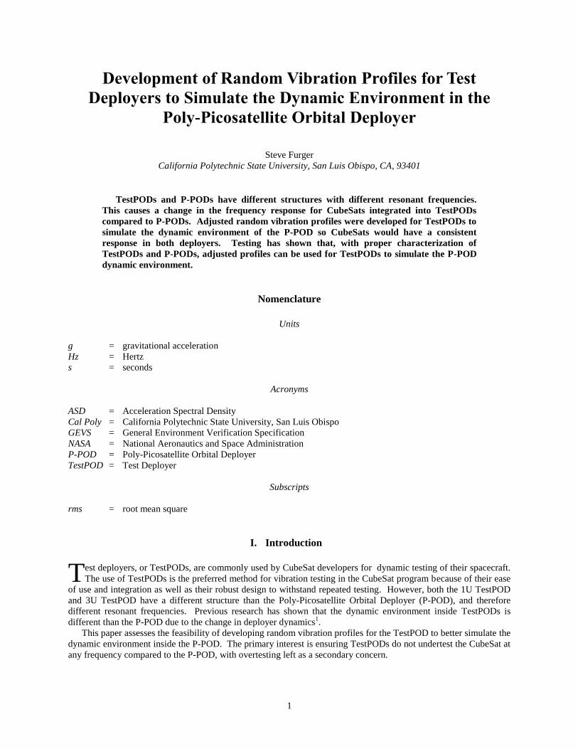
1

Development of Random Vibration Profiles for Test

Deployers to Simulate the Dynamic Environment in the

Poly-Picosatellite Orbital Deployer

Steve Furger

California Polytechnic State University, San Luis Obispo, CA, 93401

TestPODs and P-PODs have different structures with different resonant frequencies.

This causes a change in the frequency response for CubeSats integrated into TestPODs

compared to P-PODs. Adjusted random vibration profiles were developed for TestPODs to

simulate the dynamic environment of the P-POD so CubeSats would have a consistent

response in both deployers. Testing has shown that, with proper characterization of

TestPODs and P-PODs, adjusted profiles can be used for TestPODs to simulate the P-POD

dynamic environment.

Nomenclature

Units

g = gravitational acceleration

Hz = Hertz

s = seconds

Acronyms

ASD = Acceleration Spectral Density

Cal Poly = California Polytechnic State University, San Luis Obispo

GEVS = General Environment Verification Specification

NASA = National Aeronautics and Space Administration

P-POD = Poly-Picosatellite Orbital Deployer

TestPOD = Test Deployer

Subscripts

rms = root mean square

I. Introduction

est deployers, or TestPODs, are commonly used by CubeSat developers for dynamic testing of their spacecraft.

The use of TestPODs is the preferred method for vibration testing in the CubeSat program because of their ease

of use and integration as well as their robust design to withstand repeated testing. However, both the 1U TestPOD

and 3U TestPOD have a different structure than the Poly-Picosatellite Orbital Deployer (P-POD), and therefore

different resonant frequencies. Previous research has shown that the dynamic environment inside TestPODs is

different than the P-POD due to the change in deployer dynamics1.

This paper assesses the feasibility of developing random vibration profiles for the TestPOD to better simulate the

dynamic environment inside the P-POD. The primary interest is ensuring TestPODs do not undertest the CubeSat at

any frequency compared to the P-POD, with overtesting left as a secondary concern.

T

2

II. Analysis of the Dynamic Environment in CubeSat Deployers

A. Baseline Vibration Testing

Vibration testing was performed to define and compare the baseline dynamic environments inside the 1U

TestPOD, 3U TestPOD and P-POD (deployers shown in Appendix A). This data was then used to develop random

vibration profiles for TestPODs that simulate the P-POD’s dynamic environment.

Aluminum CubeSat mass models were used to measure CubeSat response due to their stiffness. Because the

CubeSat mass model’s first mode is above 2,000 Hz (see Appendix B), they can be modeled as rigid bodies inside

deployers. This provides an absolute baseline for CubeSat response to input vibration.

The NASA General Environment Verification Speciation (GEVS) random vibration profile was used as the input

to all three deployers. This profile was chosen because it provides a familiar random vibration profile for people in

the CubeSat community. Sine sweeps and low level tests were not used because testing has shown that CubeSats do

not respond linearly to input vibration magnitude. For accurate characterization of the dynamic environment, flight

vibration levels must be used. GEVS acceptance levels (9.99 grms) were chosen to provide an input vibration

magnitude around common flight levels.

Tests were run in the X and Z axes to obtain data for a fixed and unconstrained case in each deployer. For the

3U TestPOD and P-POD, tests were run to characterize the dynamic environment in different locations inside each

deployer. Table 1 shows all the tests run and their associated test numbers for baseline characterization of the

dynamic environment in the 1U TestPOD, 3U TestPOD and P-POD. The test setups are shown in Appendix C.

Table 1: Tests run for baseline characterization.

Test # Deployer Axis

1 1U TestPOD X

2 1U TestPOD Z

3-1 3U TestPOD X

3-2 3U TestPOD X

3-3 3U TestPOD X

4-1 3U TestPOD Z

4-2 3U TestPOD Z

4-3 3U TestPOD Z

5-1 P-POD X

5-2 P-POD X

6-1 P-POD Z

6-2 P-POD Z

B. Analysis of CubeSat Response in Z Axis of Deployers

The spring plungers completely constrain the CubeSats in the Z axis of all three deployers. This results in the

CubeSats resonating with the deployer’s resonant peaks. Because the P-POD has different resonant frequencies than

the 1U TestPOD and 3U TestPOD, the dynamic environment in a TestPOD is different than the dynamic

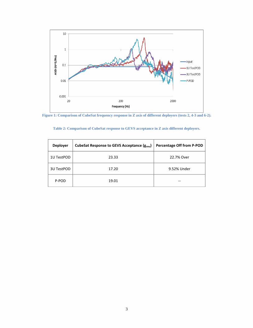
environment in the P-POD. Figure 1 shows a comparison of the frequency responses for CubeSats in the three

deployers. The overall grms for the three tests are shown in Table 2.

3

Figure 1: Comparison of CubeSat frequency response in Z axis of different deployers (tests 2, 4-3 and 6-2).

Table 2: Comparison of CubeSat response to GEVS acceptance in Z axis different deployers.

Deployer CubeSat Response to GEVS Acceptance (grms) Percentage Off from P-POD

1U TestPOD 23.33 22.7% Over

3U TestPOD 17.20 9.52% Under

P-POD 19.01 --

4

Overall, CubeSats have a higher Z axis response in the 1U TestPOD and a lower Z axis response in the 3U TestPOD

compared to the P-POD. However, both the 1U TestPOD and 3U TestPOD overtest and undertest at certain

frequency bandwidths. While the overall grms may be within 25% for all deployers, certain bandwidths can be off by

over a magnitude.

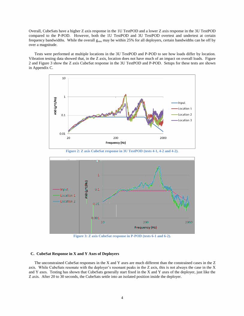
Tests were performed at multiple locations in the 3U TestPOD and P-POD to see how loads differ by location.

Vibration testing data showed that, in the Z axis, location does not have much of an impact on overall loads. Figure

2 and Figure 3 show the Z axis CubeSat response in the 3U TestPOD and P-POD. Setups for these tests are shown

in Appendix C.

Figure 2: Z axis CubeSat response in 3U TestPOD (tests 4-1, 4-2 and 4-2).

Figure 3: Z axis CubeSat response in P-POD (tests 6-1 and 6-2).

C. CubeSat Response in X and Y Axes of Deployers

The unconstrained CubeSat responses in the X and Y axes are much different than the constrained cases in the Z

axis. While CubeSats resonate with the deployer’s resonant peaks in the Z axis, this is not always the case in the X

and Y axes. Testing has shown that CubeSats generally start fixed in the X and Y axes of the deployer, just like the

Z axis. After 20 to 30 seconds, the CubeSats settle into an isolated position inside the deployer.

5

Consider vibration data from the CubeSat mass model in the X axis of the 1U TestPOD. At the beginning of the

test, the CubeSat resonates with the deployer’s resonant peak, like with the Z axis. However, as the test progresses,

the CubeSat shakes loose and becomes isolated from the deployer’s dynamics. Figure 4 shows the change in the

CubeSat response in the X axis of the 1U TestPOD over time.

Figure 4: X axis response of CubeSat in 1U TestPOD over time (test 1).

The same tests were run in the X axis of the 3U TestPOD and P-POD. These tests showed similar results, with

the CubeSat starting fixed in the deployer, then becoming isolated from the deployer after about 20 seconds. Notice

how the peaks from the CubeSat response fade over time. Figure 5 and Figure 6 show the change in CubeSat

response in the X axis of the 3U TestPOD and P-POD over time.

Figure 5: X axis response of CubeSat in 3U TestPOD over time (test 3-3).

CubeSat becomes

isolated from deployer

resonance after 10 to 20

seconds

First mode of

1U TestPOD

6

Figure 6: X axis response of CubeSat in P-POD over time (test 5-2).

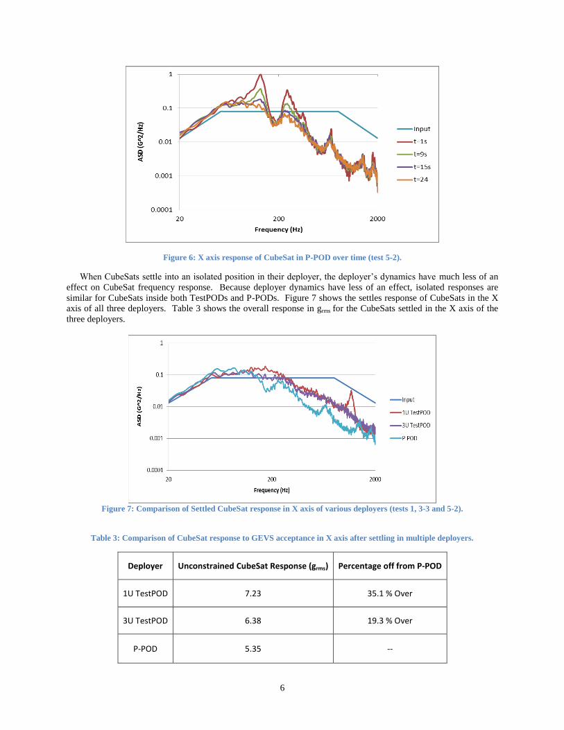
When CubeSats settle into an isolated position in their deployer, the deployer’s dynamics have much less of an

effect on CubeSat frequency response. Because deployer dynamics have less of an effect, isolated responses are

similar for CubeSats inside both TestPODs and P-PODs. Figure 7 shows the settles response of CubeSats in the X

axis of all three deployers. Table 3 shows the overall response in grms for the CubeSats settled in the X axis of the

three deployers.

Figure 7: Comparison of Settled CubeSat response in X axis of various deployers (tests 1, 3-3 and 5-2).

Table 3: Comparison of CubeSat response to GEVS acceptance in X axis after settling in multiple deployers.

Deployer Unconstrained CubeSat Response (grms) Percentage off from P-POD

1U TestPOD 7.23 35.1 % Over

3U TestPOD 6.38 19.3 % Over

P-POD 5.35 --

7

The overall grms varies more from TestPODs to P-POD in the X axis than it does in the Z axis. However, the

TestPODs have a consistently slight overtest at all frequencies in the X axis. In the Z axis, the TestPOD response

can be off by over a magnitude from P-POD response for certain frequencies.

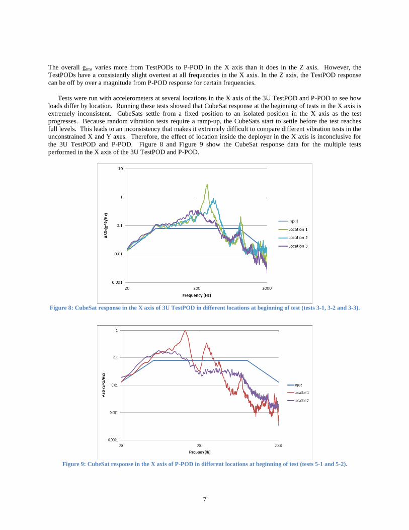
Tests were run with accelerometers at several locations in the X axis of the 3U TestPOD and P-POD to see how

loads differ by location. Running these tests showed that CubeSat response at the beginning of tests in the X axis is

extremely inconsistent. CubeSats settle from a fixed position to an isolated position in the X axis as the test

progresses. Because random vibration tests require a ramp-up, the CubeSats start to settle before the test reaches

full levels. This leads to an inconsistency that makes it extremely difficult to compare different vibration tests in the

unconstrained X and Y axes. Therefore, the effect of location inside the deployer in the X axis is inconclusive for

the 3U TestPOD and P-POD. Figure 8 and Figure 9 show the CubeSat response data for the multiple tests

performed in the X axis of the 3U TestPOD and P-POD.

Figure 8: CubeSat response in the X axis of 3U TestPOD in different locations at beginning of test (tests 3-1, 3-2 and 3-3).

Figure 9: CubeSat response in the X axis of P-POD in different locations at beginning of test (tests 5-1 and 5-2).

8

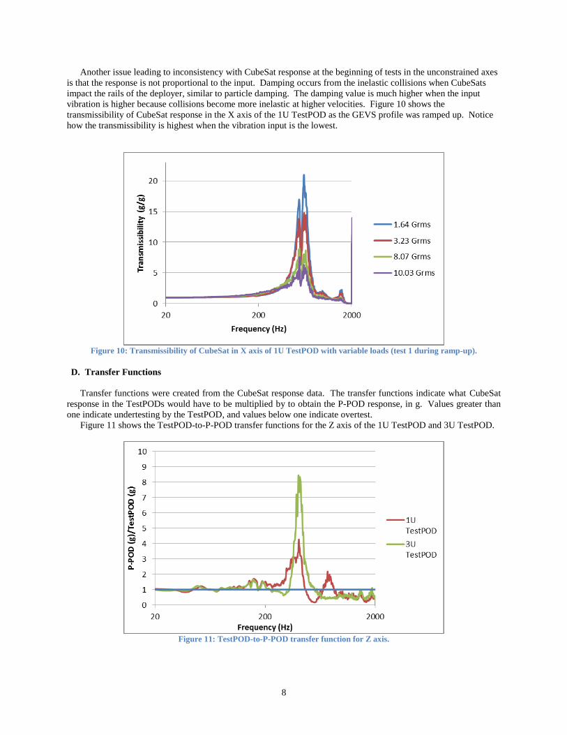
Another issue leading to inconsistency with CubeSat response at the beginning of tests in the unconstrained axes

is that the response is not proportional to the input. Damping occurs from the inelastic collisions when CubeSats

impact the rails of the deployer, similar to particle damping. The damping value is much higher when the input

vibration is higher because collisions become more inelastic at higher velocities. Figure 10 shows the

transmissibility of CubeSat response in the X axis of the 1U TestPOD as the GEVS profile was ramped up. Notice

how the transmissibility is highest when the vibration input is the lowest.

Figure 10: Transmissibility of CubeSat in X axis of 1U TestPOD with variable loads (test 1 during ramp-up).

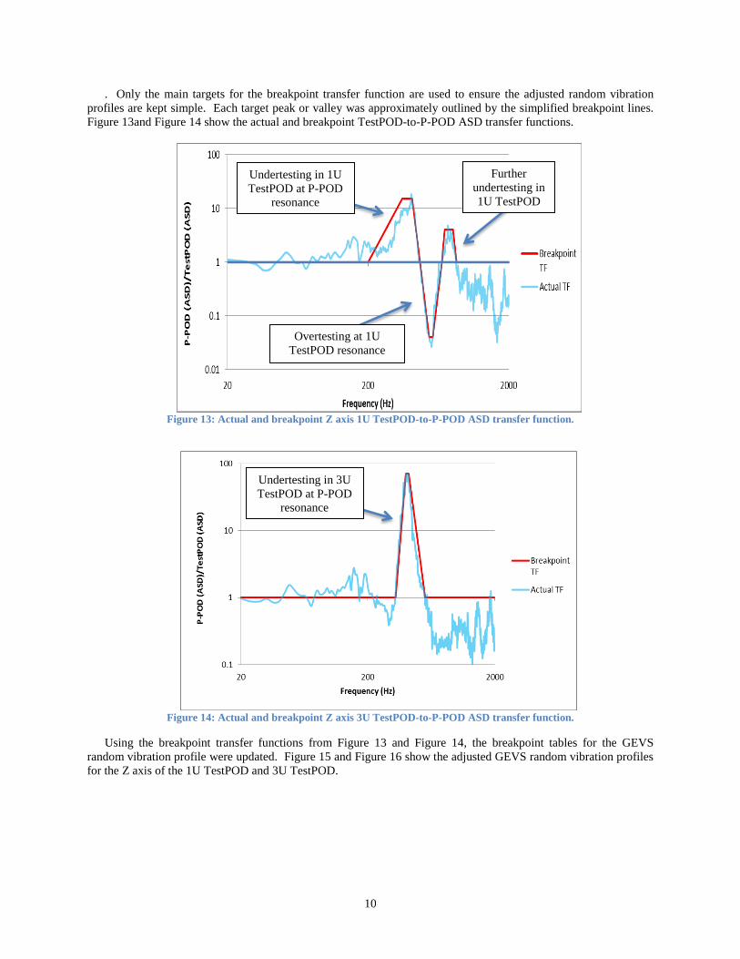
D. Transfer Functions

Transfer functions were created from the CubeSat response data. The transfer functions indicate what CubeSat

response in the TestPODs would have to be multiplied by to obtain the P-POD response, in g. Values greater than

one indicate undertesting by the TestPOD, and values below one indicate overtest.

Figure 11 shows the TestPOD-to-P-POD transfer functions for the Z axis of the 1U TestPOD and 3U TestPOD.

Figure 11: TestPOD-to-P-POD transfer function for Z axis.

9

Both TestPODs undertest CubeSats at the P-PODs natural frequency and overtest for most of the higher frequencies.

Because the CubeSats are fixed in the Z axis, there is a large amount of overtest and undertest at specific frequencies

due to the difference in deployer dynamics between the TestPODs and P-POD.

Transfer functions were much more difficult to create in the X axis. The beginnings of the tests are very

inconsistent as the CubeSats settle from a fixed position to an isolated position in the deployer. Because of this,

transfer functions were only created for settled CubeSat response. Figure 12 shows the TestPOD-to-P-POD transfer

functions for settled CubeSats in the X axis.

Figure 12: TestPOD-to-P-POD transfer function for settled CubeSats in the X axis.

The transfer functions are much less significant in the X axis than in the Z axis because the CubeSats are isolated

from deployer dynamics. It should be noted that these transfer functions are likely not proportional to the vibration

input due to the inelastic impacts of the CubeSats with the deployer rails.

III. Developing Adjusted Random Vibration Profiles

Vibration profiles were created for the X and Z axes of the 1U TestPOD and 3U TestPOD to simulate the

dynamic environment of the P-POD. The main goal of these profiles was to mitigate the TestPOD undertesting

shown in Figure 11 and Figure 12, with overtesting left as a secondary concern.

Adjusted random vibration profiles were created from acceleration spectral density TestPOD-to-P-POD transfer

functions as opposed to the regular acceleration transfer functions shown in Figure 11 and Figure 12. This was done

because random vibration profiles are in ASD units (g2/Hz). The goal was to create adjusted random vibration

profiles that have simple breakpoint tables and can be easily implemented and controlled by standard vibration

tables. For this reason, random vibration profiles could not just be multiplied by the ASD transfer functions.

Simplified “breakpoint” transfer functions would have to be created. These breakpoint transfer functions can be

applied to any random vibration profile to obtain the adjusted random vibration profile.

A. Z Axis Profile Development

Main overtest and undertest targets were selected for the breakpoint transfer functions. Both the 1U TestPOD

and 3U TestPOD undertest CubeSats in the Z axis at the frequency range of the P-POD’s resonance. This undertest

was the primary target for the adjusted random vibration profiles. For the 1U TestPOD, the overtesting at the 1U

TestPOD’s resonant frequency and the following undertesting were targeted was well. This totaled three different

targets for the 1U TestPOD-to-P-POD transfer function. No further targets were selected for the 3U TestPOD-to-P-

POD transfer function.

10

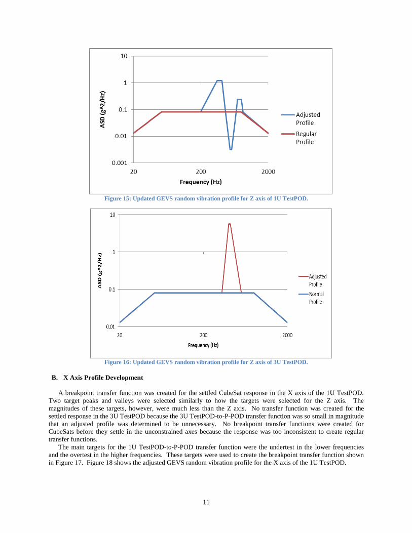
. Only the main targets for the breakpoint transfer function are used to ensure the adjusted random vibration

profiles are kept simple. Each target peak or valley was approximately outlined by the simplified breakpoint lines.

Figure 13and Figure 14 show the actual and breakpoint TestPOD-to-P-POD ASD transfer functions.

Figure 13: Actual and breakpoint Z axis 1U TestPOD-to-P-POD ASD transfer function.

Figure 14: Actual and breakpoint Z axis 3U TestPOD-to-P-POD ASD transfer function.

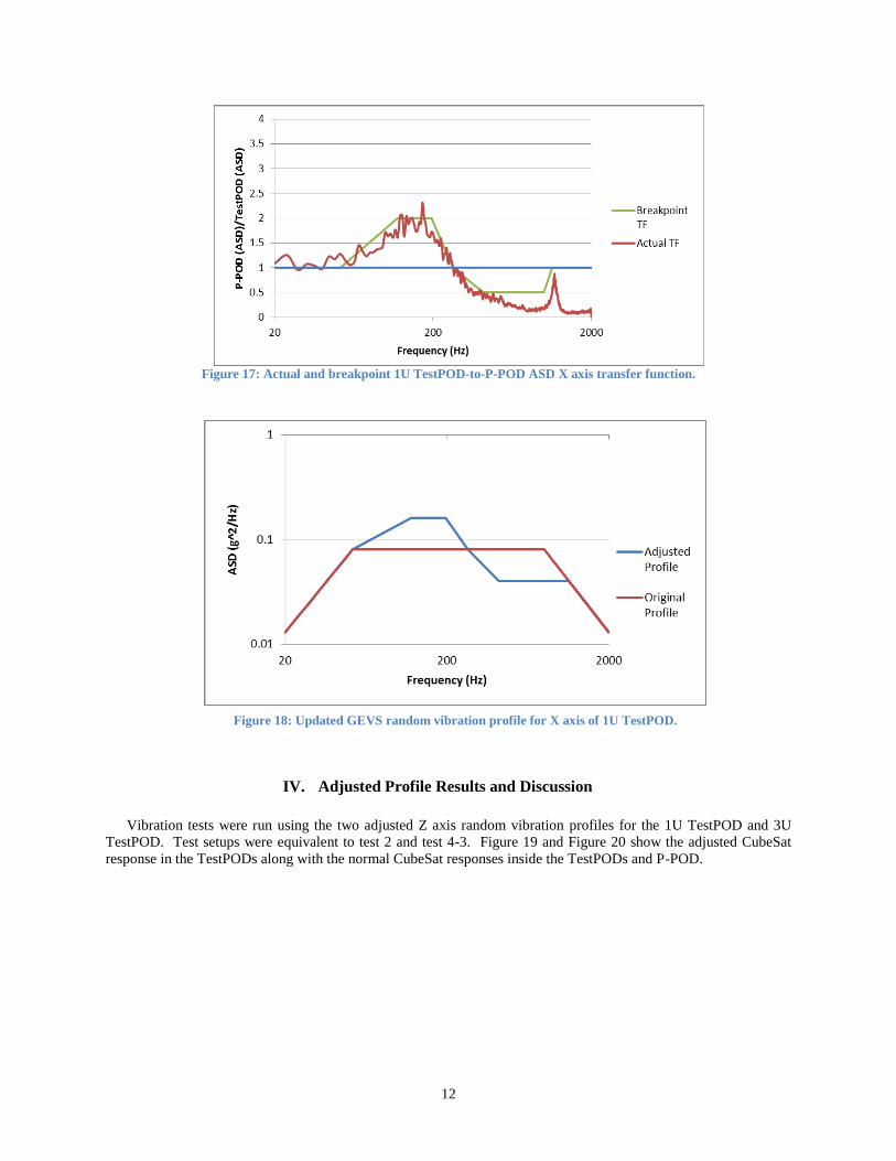
Using the breakpoint transfer functions from Figure 13 and Figure 14, the breakpoint tables for the GEVS

random vibration profile were updated. Figure 15 and Figure 16 show the adjusted GEVS random vibration profiles

for the Z axis of the 1U TestPOD and 3U TestPOD.

Undertesting in 1U

TestPOD at P-POD

resonance

Overtesting at 1U

TestPOD resonance

Further

undertesting in

1U TestPOD

Undertesting in 3U

TestPOD at P-POD

resonance

11

Figure 15: Updated GEVS random vibration profile for Z axis of 1U TestPOD.

Figure 16: Updated GEVS random vibration profile for Z axis of 3U TestPOD.

B. X Axis Profile Development

A breakpoint transfer function was created for the settled CubeSat response in the X axis of the 1U TestPOD.

Two target peaks and valleys were selected similarly to how the targets were selected for the Z axis. The

magnitudes of these targets, however, were much less than the Z axis. No transfer function was created for the

settled response in the 3U TestPOD because the 3U TestPOD-to-P-POD transfer function was so small in magnitude

that an adjusted profile was determined to be unnecessary. No breakpoint transfer functions were created for

CubeSats before they settle in the unconstrained axes because the response was too inconsistent to create regular

transfer functions.

The main targets for the 1U TestPOD-to-P-POD transfer function were the undertest in the lower frequencies

and the overtest in the higher frequencies. These targets were used to create the breakpoint transfer function shown

in Figure 17. Figure 18 shows the adjusted GEVS random vibration profile for the X axis of the 1U TestPOD.

12

Figure 17: Actual and breakpoint 1U TestPOD-to-P-POD ASD X axis transfer function.

IV. Adjusted Profile Results and Discussion

Vibration tests were run using the two adjusted Z axis random vibration profiles for the 1U TestPOD and 3U

TestPOD. Test setups were equivalent to test 2 and test 4-3. Figure 19 and Figure 20 show the adjusted CubeSat

response in the TestPODs along with the normal CubeSat responses inside the TestPODs and P-POD.

Figure 18: Updated GEVS random vibration profile for X axis of 1U TestPOD.

13

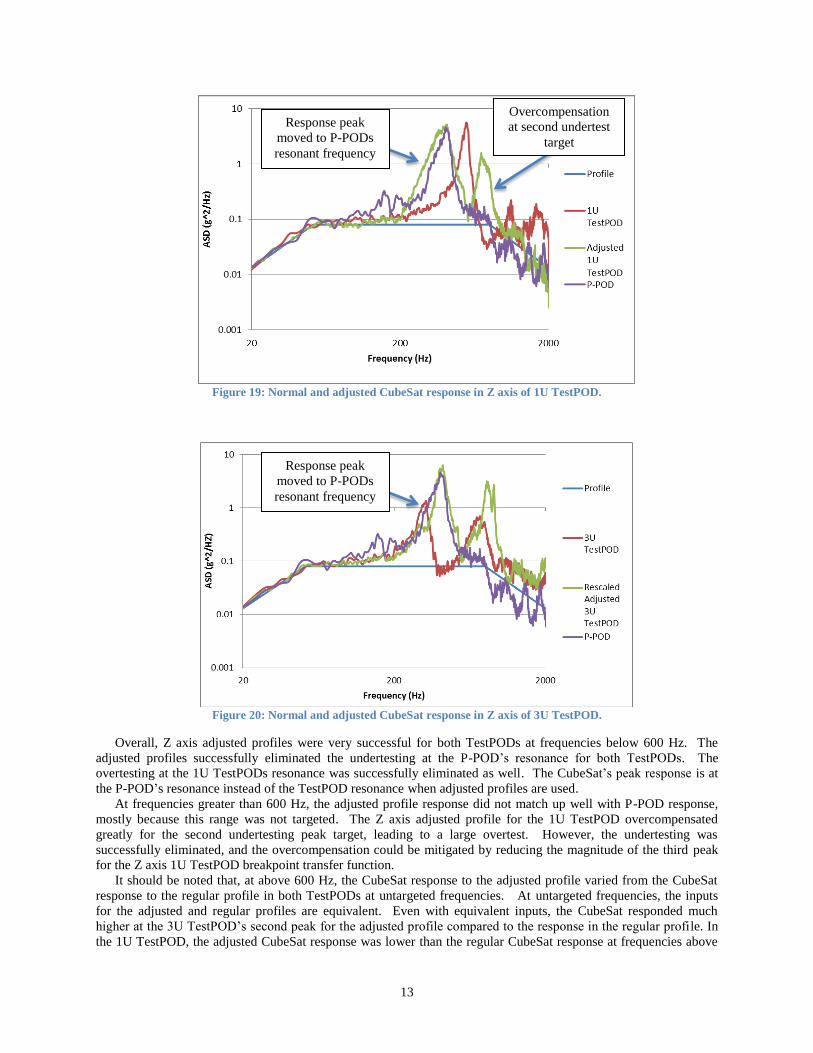
Figure 19: Normal and adjusted CubeSat response in Z axis of 1U TestPOD.

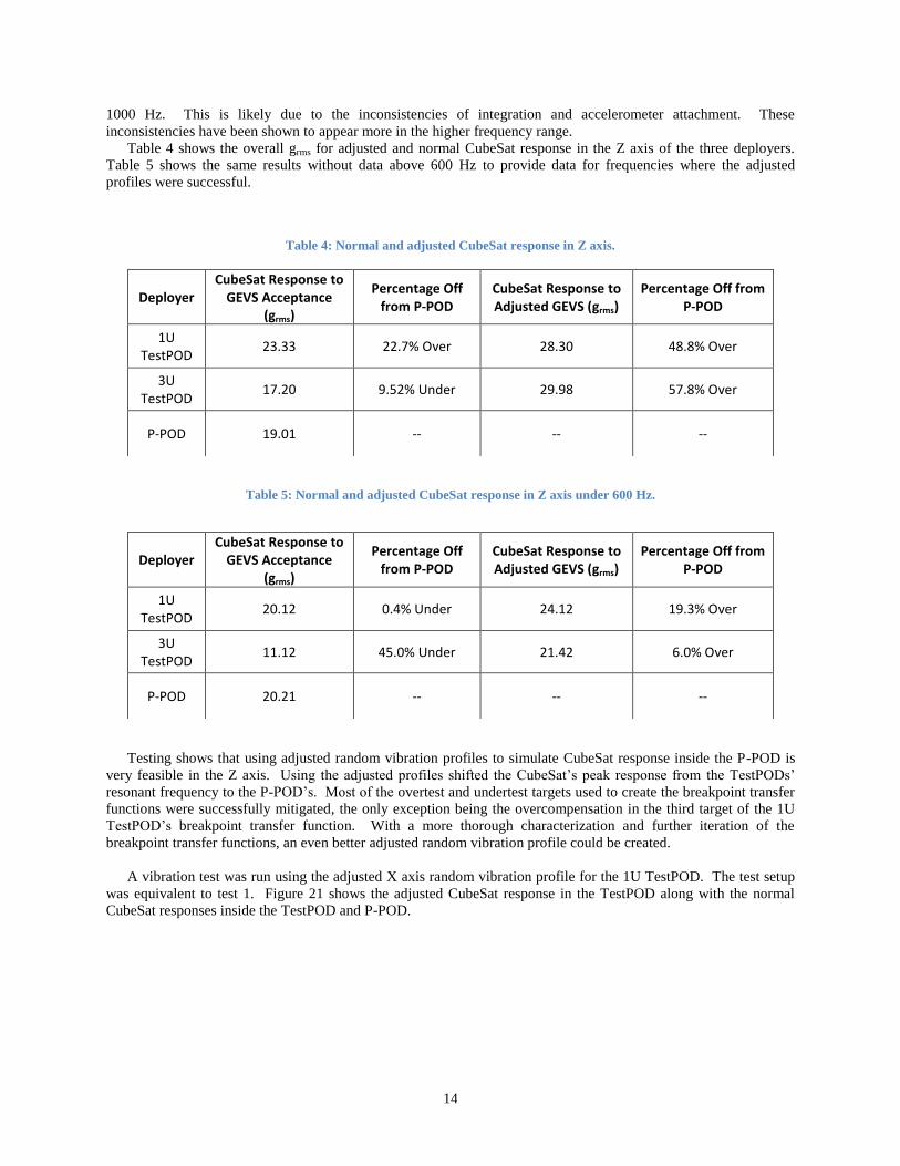
Figure 20: Normal and adjusted CubeSat response in Z axis of 3U TestPOD.

Overall, Z axis adjusted profiles were very successful for both TestPODs at frequencies below 600 Hz. The

adjusted profiles successfully eliminated the undertesting at the P-POD’s resonance for both TestPODs. The

overtesting at the 1U TestPODs resonance was successfully eliminated as well. The CubeSat’s peak response is at

the P-POD’s resonance instead of the TestPOD resonance when adjusted profiles are used.

At frequencies greater than 600 Hz, the adjusted profile response did not match up well with P-POD response,

mostly because this range was not targeted. The Z axis adjusted profile for the 1U TestPOD overcompensated

greatly for the second undertesting peak target, leading to a large overtest. However, the undertesting was

successfully eliminated, and the overcompensation could be mitigated by reducing the magnitude of the third peak

for the Z axis 1U TestPOD breakpoint transfer function.

It should be noted that, at above 600 Hz, the CubeSat response to the adjusted profile varied from the CubeSat

response to the regular profile in both TestPODs at untargeted frequencies. At untargeted frequencies, the inputs

for the adjusted and regular profiles are equivalent. Even with equivalent inputs, the CubeSat responded much

higher at the 3U TestPOD’s second peak for the adjusted profile compared to the response in the regular profile. In

the 1U TestPOD, the adjusted CubeSat response was lower than the regular CubeSat response at frequencies above

Response peak

moved to P-PODs

resonant frequency

Overcompensation

at second undertest

target

Response peak

moved to P-PODs

resonant frequency

14

1000 Hz. This is likely due to the inconsistencies of integration and accelerometer attachment. These

inconsistencies have been shown to appear more in the higher frequency range.

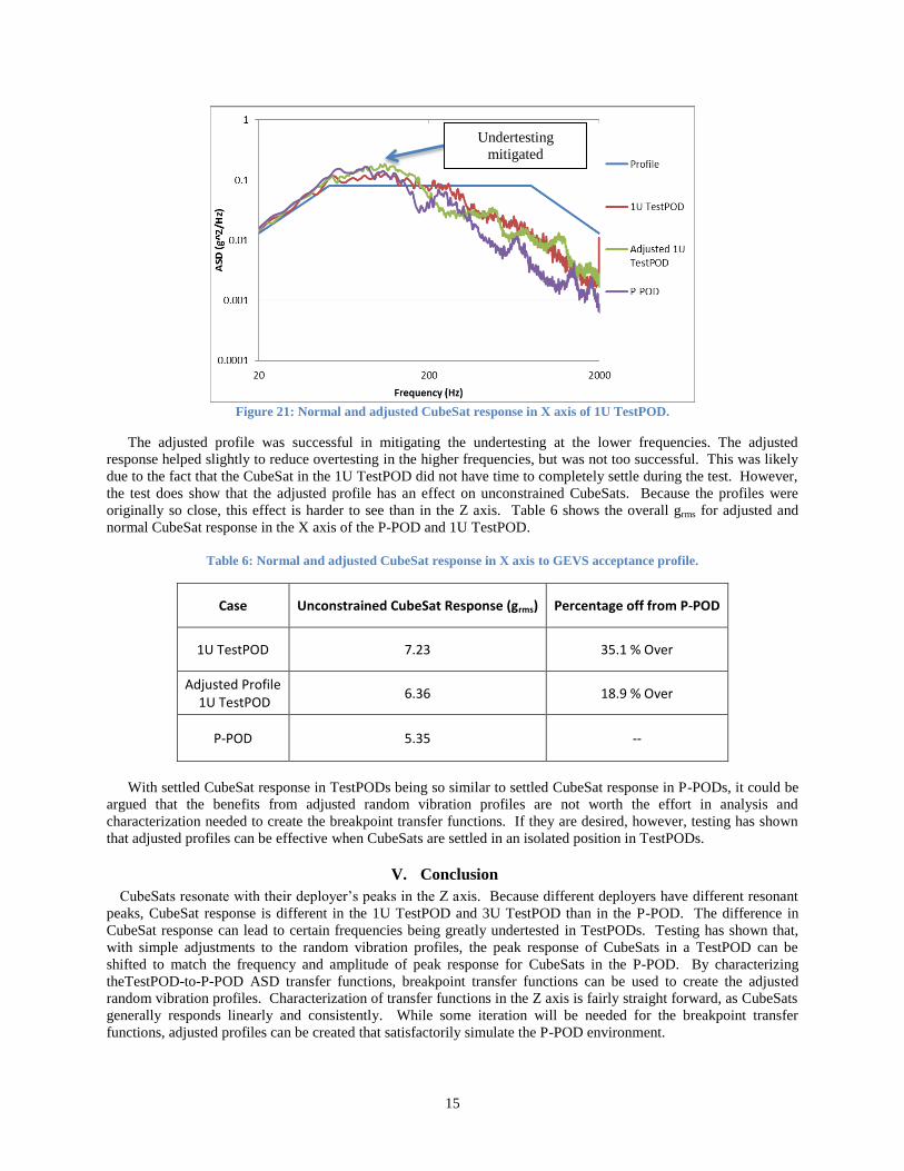
Table 4 shows the overall grms for adjusted and normal CubeSat response in the Z axis of the three deployers.

Table 5 shows the same results without data above 600 Hz to provide data for frequencies where the adjusted

profiles were successful.

Table 4: Normal and adjusted CubeSat response in Z axis.

Table 5: Normal and adjusted CubeSat response in Z axis under 600 Hz.

Testing shows that using adjusted random vibration profiles to simulate CubeSat response inside the P-POD is

very feasible in the Z axis. Using the adjusted profiles shifted the CubeSat’s peak response from the TestPODs’

resonant frequency to the P-POD’s. Most of the overtest and undertest targets used to create the breakpoint transfer

functions were successfully mitigated, the only exception being the overcompensation in the third target of the 1U

TestPOD’s breakpoint transfer function. With a more thorough characterization and further iteration of the

breakpoint transfer functions, an even better adjusted random vibration profile could be created.

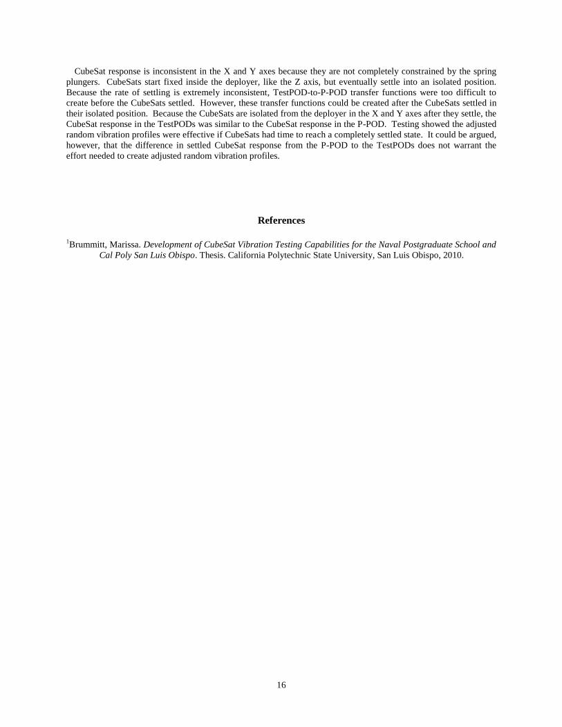
A vibration test was run using the adjusted X axis random vibration profile for the 1U TestPOD. The test setup

was equivalent to test 1. Figure 21 shows the adjusted CubeSat response in the TestPOD along with the normal

CubeSat responses inside the TestPOD and P-POD.

Deployer CubeSat Response to

GEVS Acceptance (grms)

Percentage Off from P-POD

CubeSat Response to Adjusted GEVS (grms)

Percentage Off from P-POD

1U TestPOD

23.33 22.7% Over 28.30 48.8% Over

3U TestPOD

17.20 9.52% Under 29.98 57.8% Over

P-POD 19.01 -- -- --

Deployer CubeSat Response to

GEVS Acceptance (grms)

Percentage Off from P-POD

CubeSat Response to Adjusted GEVS (grms)

Percentage Off from P-POD

1U TestPOD

20.12 0.4% Under 24.12 19.3% Over

3U TestPOD

11.12 45.0% Under 21.42 6.0% Over

P-POD 20.21 -- -- --

15

Figure 21: Normal and adjusted CubeSat response in X axis of 1U TestPOD.

The adjusted profile was successful in mitigating the undertesting at the lower frequencies. The adjusted

response helped slightly to reduce overtesting in the higher frequencies, but was not too successful. This was likely

due to the fact that the CubeSat in the 1U TestPOD did not have time to completely settle during the test. However,

the test does show that the adjusted profile has an effect on unconstrained CubeSats. Because the profiles were

originally so close, this effect is harder to see than in the Z axis. Table 6 shows the overall grms for adjusted and

normal CubeSat response in the X axis of the P-POD and 1U TestPOD.

Table 6: Normal and adjusted CubeSat response in X axis to GEVS acceptance profile.

Case Unconstrained CubeSat Response (grms) Percentage off from P-POD

1U TestPOD 7.23 35.1 % Over

Adjusted Profile 1U TestPOD

6.36 18.9 % Over

P-POD 5.35 --

With settled CubeSat response in TestPODs being so similar to settled CubeSat response in P-PODs, it could be

argued that the benefits from adjusted random vibration profiles are not worth the effort in analysis and

characterization needed to create the breakpoint transfer functions. If they are desired, however, testing has shown

that adjusted profiles can be effective when CubeSats are settled in an isolated position in TestPODs.

V. Conclusion

CubeSats resonate with their deployer’s peaks in the Z axis. Because different deployers have different resonant

peaks, CubeSat response is different in the 1U TestPOD and 3U TestPOD than in the P-POD. The difference in

CubeSat response can lead to certain frequencies being greatly undertested in TestPODs. Testing has shown that,

with simple adjustments to the random vibration profiles, the peak response of CubeSats in a TestPOD can be

shifted to match the frequency and amplitude of peak response for CubeSats in the P-POD. By characterizing

theTestPOD-to-P-POD ASD transfer functions, breakpoint transfer functions can be used to create the adjusted

random vibration profiles. Characterization of transfer functions in the Z axis is fairly straight forward, as CubeSats

generally responds linearly and consistently. While some iteration will be needed for the breakpoint transfer

functions, adjusted profiles can be created that satisfactorily simulate the P-POD environment.

Undertesting

mitigated

16

CubeSat response is inconsistent in the X and Y axes because they are not completely constrained by the spring

plungers. CubeSats start fixed inside the deployer, like the Z axis, but eventually settle into an isolated position.

Because the rate of settling is extremely inconsistent, TestPOD-to-P-POD transfer functions were too difficult to

create before the CubeSats settled. However, these transfer functions could be created after the CubeSats settled in

their isolated position. Because the CubeSats are isolated from the deployer in the X and Y axes after they settle, the

CubeSat response in the TestPODs was similar to the CubeSat response in the P-POD. Testing showed the adjusted

random vibration profiles were effective if CubeSats had time to reach a completely settled state. It could be argued,

however, that the difference in settled CubeSat response from the P-POD to the TestPODs does not warrant the

effort needed to create adjusted random vibration profiles.

References

1Brummitt, Marissa. Development of CubeSat Vibration Testing Capabilities for the Naval Postgraduate School and

Cal Poly San Luis Obispo. Thesis. California Polytechnic State University, San Luis Obispo, 2010.

17

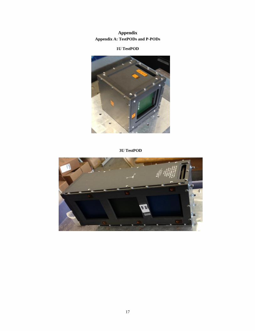
Appendix

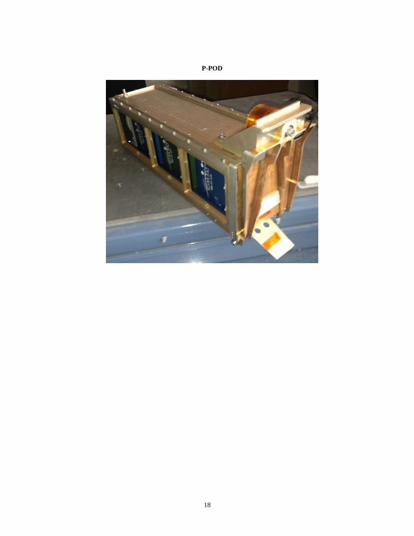
Appendix A: TestPODs and P-PODs

1U TestPOD

3U TestPOD

18

P-POD

19

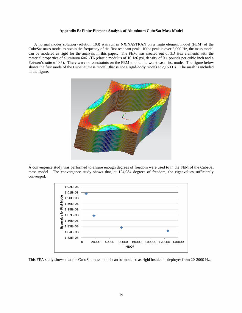
Appendix B: Finite Element Analysis of Aluminum CubeSat Mass Model

A normal modes solution (solution 103) was run in NX/NASTRAN on a finite element model (FEM) of the

CubeSat mass model to obtain the frequency of the first resonant peak. If the peak is over 2,000 Hz, the mass model

can be modeled as rigid for the analysis in this paper. The FEM was created out of 3D Hex elements with the

material properties of aluminum 6061-T6 (elastic modulus of 10.1e6 psi, density of 0.1 pounds per cubic inch and a

Poisson’s ratio of 0.3). There were no constraints on the FEM to obtain a worst case first mode. The figure below

shows the first mode of the CubeSat mass model (that is not a rigid-body mode) at 2,160 Hz. The mesh is included

in the figure.

A convergence study was performed to ensure enough degrees of freedom were used to in the FEM of the CubeSat

mass model. The convergence study shows that, at 124,984 degrees of freedom, the eigenvalues sufficiently

converged.

This FEA study shows that the CubeSat mass model can be modeled as rigid inside the deployer from 20-2000 Hz.

20

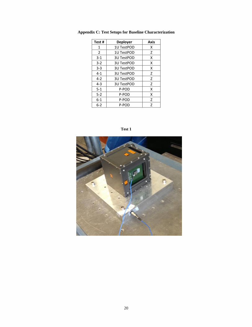
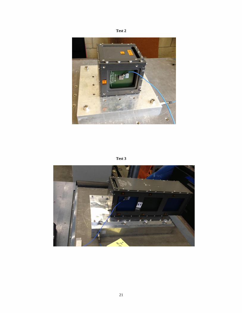
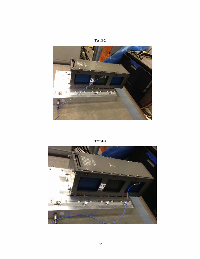
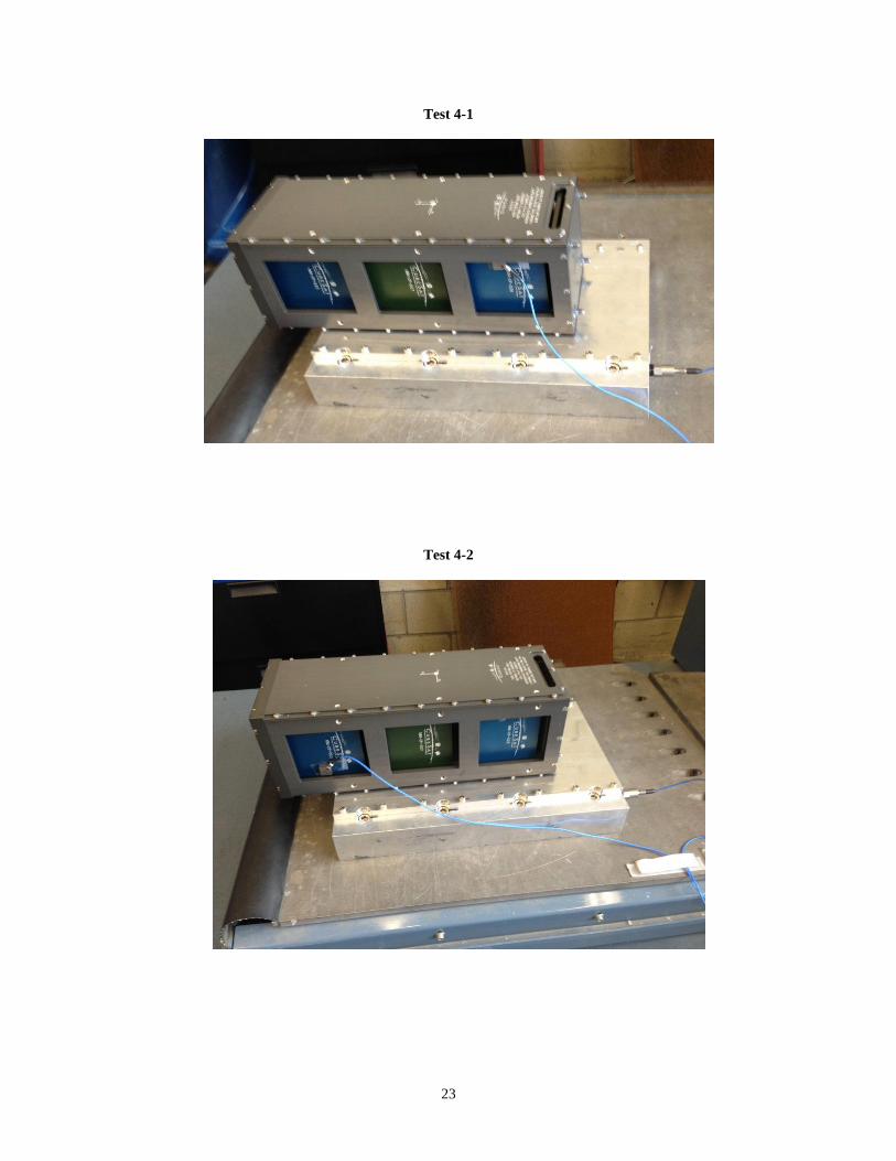
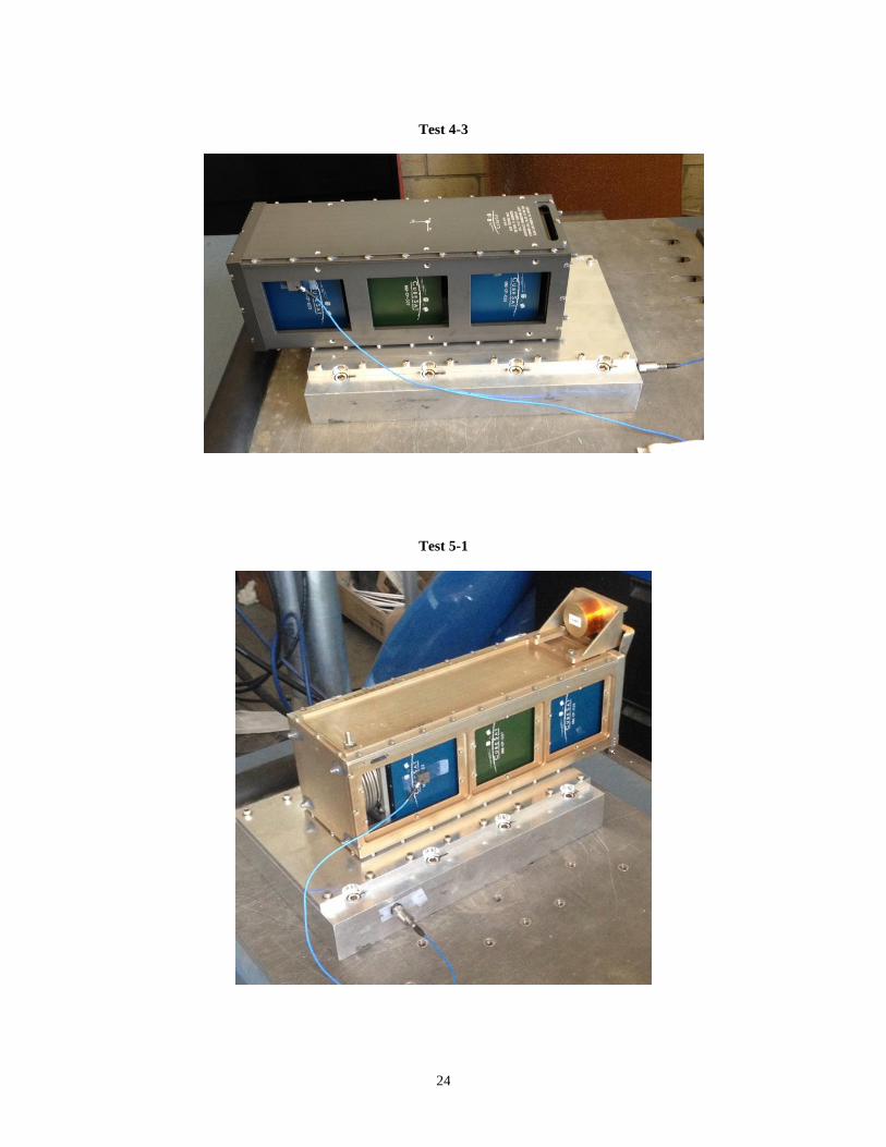
Appendix C: Test Setups for Baseline Characterization

Test # Deployer Axis

1 1U TestPOD X

2 1U TestPOD Z

3-1 3U TestPOD X

3-2 3U TestPOD X

3-3 3U TestPOD X

4-1 3U TestPOD Z

4-2 3U TestPOD Z

4-3 3U TestPOD Z

5-1 P-POD X

5-2 P-POD X

6-1 P-POD Z

6-2 P-POD Z

Test 1

21

Test 2

Test 3

22

Test 3-2

Test 3-3

23

Test 4-1

Test 4-2

24

Test 4-3

Test 5-1

25

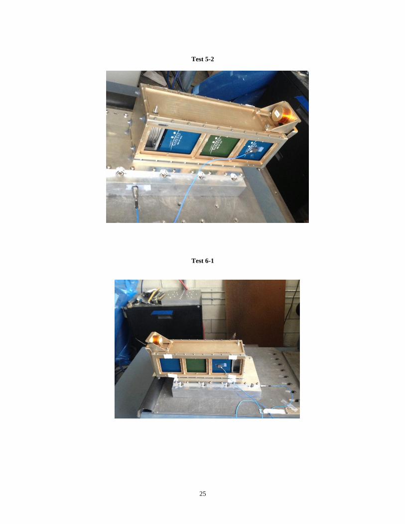
Test 5-2

Test 6-1

26

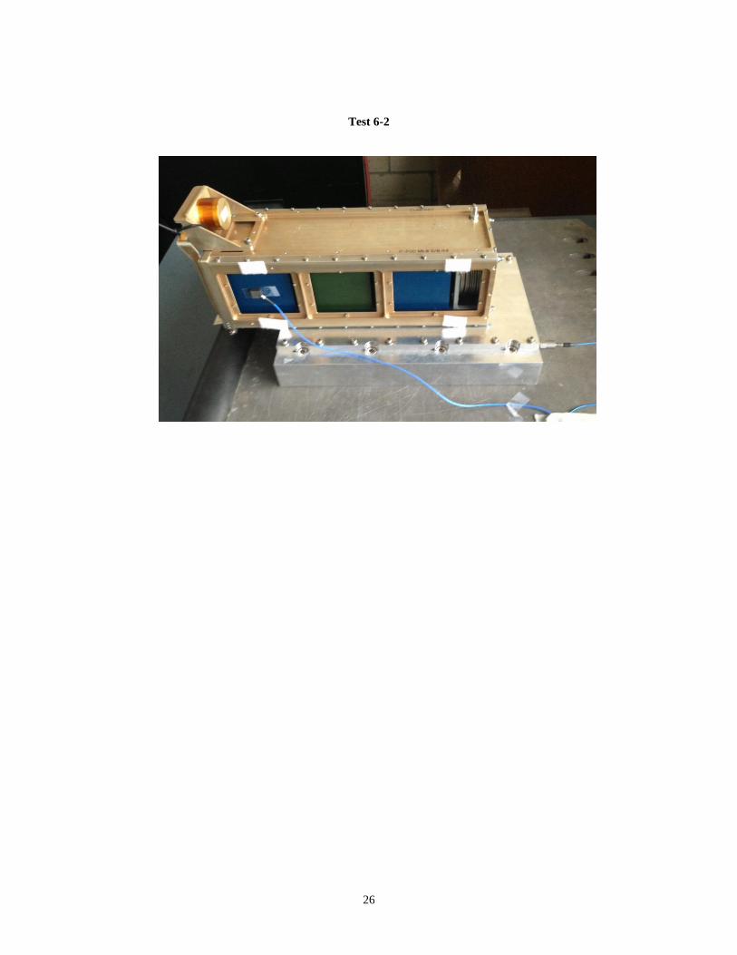
Test 6-2