Master’s DissertationStructuralMechanics

KARL BONDESSON

DEVELOPMENT OFMETHODOLOGY FOR GENERATINGRESPONSE SPECTRA FORDECOUPLED SMALLBORE PIPING

DEPARTMENT OF CONSTRUCTION SCIENCES

DIVISION OF STRUCTURAL MECHANICS

ISRN LUTVDG/TVSM--14/5201--SE (1-52) | ISSN 0281-6679

MASTER’S DISSERTATION

Supervisors: PER-ERIK AUSTRELL, Assoc. prof., Div. of Structural Mechanics, LTH, Lund and ANDERS BLOM, AREVA NP Uddcomb AB.

Examiner: KENT PERSSON, PhD, Div. of Structural Mechanics, LTH, Lund.

Copyright © 2014 Division of Structural MechanicsFaculty of Engineering (LTH), Lund University, Sweden.

Printed by Media-Tryck LU, Lund, Sweden, November 2014 (Pl).

For information, address:Div. of Structural Mechanics, LTH, Lund University, Box 118, SE-221 00 Lund, Sweden.

Homepage: http://www.byggmek.lth.se

KARL BONDESSON

DEVELOPMENT OFMETHODOLOGY FOR GENERATING

RESPONSE SPECTRA FORDECOUPLED SMALLBORE PIPING

1

Preface This master’s dissertation concludes a five year civil engineering master program at Lund

University. This project has sparked a further interest of mine in the field of structural

analysis. I would like to thank Anders Blom at Areva NP Uddcomb in Helsingborg for his

continued support and interest in this research. I would also like to thank Per-Erik Austrell

and Kent Persson at the division of Structural Mechanics at Lund University.

Lund, October 2014

2

Abstract In nuclear piping engineering, the response spectrum method of analysis is widely used to

analyze piping systems. The matter of combining modal responses is of great interest.

Complications may occur with the response spectrum method for large systems. Examples are

convergence issues and something called twin-mode effects that may overestimate the effects

on the system. This master thesis investigates the possibility of separating small parts of

piping systems, thus reducing the original system in size, and analyzing the separated systems

independently by loading them with a modified response spectrum based around a dynamic

amplification factor. The process of calculating the modified response spectrum is automated

by the development of an application using Python.

The modeling of the piping systems is done in Pipestress, which is a commonly used

computer software for design of pipes at nuclear power plants. Different modal combination

methods and certain modeling issues are investigated and finally the stress in the original and

the separated system is calculated and compared.

There is no experimental data to compare the results to, but the method of separating systems

with a modified response spectrum shows some promise, even though further investigation is

needed.

3

Table of Contents

PREFACE ............................................................................................................ 1

ABSTRACT ......................................................................................................... 2

1. INTRODUCTION ........................................................................................... 5

1.1 Background ......................................................................................................................... 5

1.2 Objective ............................................................................................................................. 5

1.3 Areva NP Uddcomb ........................................................................................................... 5

1.4 Limitations .......................................................................................................................... 6

2. THEORY OF DYNAMICS ............................................................................ 7

2.1 Equation of motion ............................................................................................................. 7

2.2 Modal analysis .................................................................................................................... 7

2.3 Response spectrum ............................................................................................................. 8

2.4 The response spectrum method of analysis .................................................................... 11

2.5 Summation methods ......................................................................................................... 12

2.6 Twin mode problem ......................................................................................................... 14

2.7 Choice of superposition method ...................................................................................... 14

3. METHOD ....................................................................................................... 16

3.1 Modified response spectrum ........................................................................................... 16

3.2 Using the dynamic amplification factor to create a spectrum ..................................... 19

3.3 Developing an automated process of calculating the modified response spectrum ... 20

4. MODELLING IN PIPESTRESS ................................................................. 21

4.1 Investigating the method ................................................................................................. 21

4.2 Models used ....................................................................................................................... 22

4

4.2.1 Model 1 ....................................................................................................................... 22

4.2.2 Model 2 ....................................................................................................................... 23

4.3 Response spectra used ...................................................................................................... 25

4.4 Modelling of connection point ......................................................................................... 25

4.5 Example of summation with results from PipeStress ................................................... 26

4.5.1 ABSSUM example ...................................................................................................... 27

4.5.2 SRSS example ............................................................................................................. 28

4.5.3 CQC example .............................................................................................................. 28

5. RESULTS ....................................................................................................... 29

5.1 Model 1 .............................................................................................................................. 29

5.1.1 Modified response spectrum ....................................................................................... 29

5.1.2 Modified response spectrum comparison .................................................................... 32

5.1.3 Anchor with spring stiffness ....................................................................................... 32

5.1.4 Summary Model 1 ....................................................................................................... 33

5.2 Model 2 .............................................................................................................................. 35

5.2.1 Modified response spectrum ....................................................................................... 35

5.2.2 Modified response spectrum comparison .................................................................... 39

5.2.3 Spring stiffness ............................................................................................................ 39

5.2.4 Summary Model 2 ....................................................................................................... 40

6. CONCLUSIONS ............................................................................................ 42

7. FUTURE RESEARCH ................................................................................. 44

REFERENCES .................................................................................................. 45

APPENDIX A .................................................................................................... 46

Calculation results .................................................................................................................. 46

Model 1 ................................................................................................................................ 46

Model 2 ................................................................................................................................ 49

5

1. Introduction

1.1 Background

In 2013, a master thesis work was commenced in association with Areva NP Uddcomb that

should investigate different methods that could allow for the separation of piping systems

with response spectrum loads. The reasons for wanting to separate small pipes from larger

piping systems are numerous. For example, a large system is approximately unaffected by the

removing of the small pipe if the small pipe has an area moment of inertia that is less than

1/25th than that of the larger system (Welding Research Council, 1984). Also, leaving the

small pipe in the larger model can have several calculation complications; once models

become too large, problems may occur with convergence. Leaving a small pipe in the model

can introduce a small mass difference that can lead to something called twin-modes, which in

turn lead to over-conservative responses in the analysis.

Since the larger system can be calculated separately, the question of verifying the small pipe

on its own remains. When the load is applied as a response spectrum, there is no time history

information in the connection point where the small pipe is connected to the large system, and

a load case for the small pipe cannot be calculated in a simple, obvious manner.

The previous master thesis investigated a number of methods of approximating the load

effects on the small pipe; static approximations, replacing the small pipe with a point mass,

time history approximations and finally a modified response spectrum. The thesis concluded

in 2014, among other things, that a modified response spectrum method could work as an

approximation, but it needed further verification and deeper investigation in several areas.

1.2 Objective

The main objective is to investigate and develop calculation tools for a method to separate

smaller pipes from models of larger piping systems. This thesis focuses on a method of

separation based on the assumption that a small pipe will have a very small, assumed

insignificant, effect on the larger systems behavior. The small pipe is simply removed from

the model, and will instead require separate analysis. To analyze the small pipe, a response

spectrum load is created based on the large model’s response. Data needed for creating the

response spectrum will be collected from results generated by the commercial FE-program

PipeStress using real piping models.

To carry out the calculations and investigate the problem, an automated process for collecting

the data will have to be developed as part of the thesis.

1.3 Areva NP Uddcomb

In 1970 Uddcomb AB Sweden was founded by the Swedish government, Uddeholm AB and

Combustion Engineering as owners. Uddcomb AB manufactured many reactor pressure

vessels to the nuclear power plants in Sweden, but also exported to Finland and Germany. The

company went through some changes over the years, and finally in 2005 Uddcomb

Engineering AB became a subsidiary of AREVA NP.

6

AREVA is a French multinational company specializing in nuclear and renewable energy.

AREVA has around 45 000 employees as of 2013. The company is divided into 5 business

areas:

Mining

Front End

Reactors and Services

Back End

Renewable energy

AREVA NP Uddcomb has around 170 employees and the revenue for 2013 was around 540

million SEK. The company is located in Helsingborg and Karlskrona.

1.4 Limitations

The following limitations apply

Linear elastic isotropic material properties are assumed

Damping constants ≤ 0.05

Cut-off frequency chosen as 100 Hz in modal analysis

Four modal superposition methods investigated; absolute summation, square root of

sum of squares, NRC 10 % grouping method, complete quadratic combination

No coupled stiffnesses considered in modelling of anchor points

No reference time-history calculations are executed

7

2. Theory of dynamics

2.1 Equation of motion

The basis for the theory of dynamics is the equation of motion. The equation of motion for a

single degree of freedom (SDOF) mass-stiffness system with damping is

𝑚�̈� + 𝑐�̇� + 𝑘𝑢(𝑡) = 𝑝(𝑡)

(2.1)

𝑢, �̇�, �̈� is displacement, velocity and acceleration as a function of time and 𝑚, 𝑐 and 𝑘 is

mass, damping and stiffness, and 𝑝(𝑡) is the applied force.

Dividing this equation by m gives another useful formulation of the equation of motion

�̈� + 2𝜁𝜔𝑛�̇� + 𝜔𝑛2𝑢 = 𝑝(𝑡)

(2.2)

𝜔𝑛 = √𝑘

𝑚 is the natural frequency and 𝜁 =

𝑐

2𝑚𝜔𝑛 is the critical damping ratio.

2.2 Modal analysis

For a multi-degree of freedom system (MDOF) without damping, free vibration (no applied

loads) is described by Eq. 2.3.

𝑴�̈� + 𝑲𝒖 = 𝟎

(2.3)

𝑴 and 𝑲 are the mass and stiffness matrices and 𝒖 and �̈� are the displacement and relative

acceleration vectors

When assuming harmonic motion, the mode shape displacement can be written as

𝑢 = 𝐴𝑐𝑜𝑠(𝜔𝑛𝑡)𝚽

(2.4)

𝜔𝑛 holds the natural frequencies and 𝚽 is the mode shape matrix.

Any deformed shape of a structure can be made up of a linear combination of these mode

shapes. Eq. 2.5 can then be formulated as

(𝑲 − 𝜔𝑛𝟐𝑴)𝚽 = 𝟎 (2.5)

Eq. 2.5 is an eigenvalue problem and can be solved by

𝑑𝑒𝑡(𝑲 − 𝜔𝑛2𝑴) = 𝟎 (2.6)

Several eigenfrequencies are computed from Eq. 2.6, and the corresponding modes are

calculated from Eq. 2.5. The analysis of a mass-stiffness system without loading that

generates, among other things, the eigenfrequencies and eigenmodes is called modal analysis.

The displacement 𝒖(𝑡) can be described as a superposition of all modes of vibration, each

corresponding to a natural frequency.

8

𝒖(𝑡) =∑𝑞𝑖(𝑡)𝜙𝑖

(2.7)

𝑞𝑖(𝑡) is a scalar time function and 𝜙𝑖 is the mode shape vector

Any motion can be represented by a linear combination of the systems modes and their time

functions, as long as the system is considered linear.

The equation of motion for a MDOF system can be rewritten by using Eq. 2.7 and

premultiplying the terms with 𝜙𝑖𝑇. It can be shown that 𝜙𝑗

𝑇𝑴𝜙𝑖 = 0 and 𝜙𝑗𝑇𝑲𝜙𝑖 = 0 when

𝑖 ≠ 𝑗 (Chopra, 1995). In other words, the modes are orthogonal. Since only the terms with

𝑖 = 𝑗 remain, the equations become uncoupled.

∑𝜙𝑖𝑇𝑴𝜙𝑖�̈�𝑖(𝑡) +∑𝜙𝑖

𝑇𝑪𝜙𝑖�̇�𝑖(𝑡) +∑𝜙𝑖𝑇𝑲𝜙𝑖𝑞𝑖(𝑡) = 𝜙𝑖

𝑇𝒑(𝑡) (2.8)

Each equation can be solved on its own after a modal analysis has been performed, and only

𝑞𝑖 and its derivatives are unknown. The equations can be solved either by a time stepping

method like Newmark’s method or the Central Difference Method, or using a convolution

integral like Duhamel’s integral. Once solved, simply transform back from 𝑞 to 𝒖 by using

Eq. 2.7 to get the displacement.

An advantage of this formulation is the fact that a systems behavior can be described

accurately without all the mode shapes. The ones with low frequencies govern the motion to

such a degree that many higher frequency modes can be left out of the calculation.

For further information on these subjects please refer to (Clough & Penzien, 1993) or

(Chopra, 1995).

2.3 Response spectrum

A response spectrum is a plot of the maximum response of a number of idealized single-

degree-of-freedom oscillators (see Figure 2.1) with certain natural frequencies, subjected to a

dynamic load, e.g. ground acceleration �̈�𝑔.

Figure 2.1. Oscillator

The SDOF system in Figure 2.1 is described by

𝑚�̈� + 𝑐�̇� + 𝑘𝑢 = −𝑚�̈�𝑔 (2.9)

9

The equation be can be rewritten (see Eq. 2.2) as

�̈� + 2𝜁𝜔𝑛�̇� + 𝜔𝑛2𝑢 = −�̈�𝑔 (2.10)

By solving the equation of motion for systems with different natural frequencies 𝜔𝑛 and

damping constants 𝜁, and analyzing the maximum response (acceleration, velocity or

displacement), a response spectrum can be created.

To create a ground motion deformation response spectrum, 𝑆𝑑(𝜁, 𝜔), for a given ground

motion, one follows the steps below (Chopra, 1995):

1. Numerically define the ground acceleration �̈�𝑔(𝑡)

2. Select the natural frequency, 𝜔𝑛, and the damping constant, 𝜁, of the SDOF system

3. Use a numerical method to calculate the deformation response as a function of time

4. Register the peak value of the deformation response for the SDOF system

5. Repeat steps 2-4 for other damping constants and natural frequencies to create a range

of interest

6. Plot the results

Figure 2.2. Creation of deformation response spectrum (Chopra, 1995)

Figure 2.2(b) show the numerically calculated deformation response history, u(t), for a

number of SDOF oscillators with certain natural periods and the damping constant 2%, for the

10

measured ground motion from the El Centro earthquake Figure 2.2(a). The deformation

response spectrum is also presented in Figure 2.2(c).

Using Eq. 2.11 the corresponding pseudo-velocity and pseudo-acceleration response spectrum

is created. Figure 2.3 show these spectra.

1

𝜔2∙ 𝑆𝑝𝑎(𝜁, 𝜔) ≈

1

𝜔∙ 𝑆𝑝𝑣(𝜁, 𝜔) ≈ 𝑆𝑑(𝜁, 𝜔)

(2.11)

This not the actual velocity or acceleration, since they are based on the relative displacement

between the moving ground and the moving mass of the oscillator, and they are instead called

pseudo-velocity and pseudo-acceleration response spectrum respectively.

Note that while the spectra from (Chopra, 1995) are plots of response against natural period,

the response can also be plotted against natural frequency using the relationship 𝑇𝑛 =2𝜋

𝜔𝑛.

Figure 2.3. (Chopra, 1995)

11

There are different types of response spectra referred to in nuclear piping design. The ground

motion response spectrum refers to the response of a building standing on the ground. The

building response is simulated by idealized SDOF oscillators while the ground is subjected to

dynamic loads such as earthquake loads.

The in-building response spectrum refers to the response in structures attached to the

building. The piping system is simulated by idealized single-degree-of-freedom oscillators

while the building is subjected to dynamic loads. See Figure 2.4.

Figure 2.4. The earthquake can be represented by a ground motion response spectrum. The

theoretical SDOF oscillators inside a building are used to create an in-building response spectrum.

(Smith & Van Laan, 1987)

2.4 The response spectrum method of analysis

The equation of motion for an MDOF system with ground motion acceleration is

𝑴�̈� + 𝑪�̇� + 𝑲𝒖 = −𝑴𝑰�̈�𝑔 (2.12)

𝑰 is the identity matrix.

Using the mode shapes to perform modal transformation, Eq. 2.12 can be rewritten according

to (Datta, 2010) as

�̈�𝑖 + 2𝜁𝑖𝜔𝑖�̇�𝑖 + 𝜔𝑖

2𝑢𝑖 = −𝜙𝑖𝑇𝑴𝑰

𝜙𝑖𝑇𝑴𝜙𝑖

�̈�𝑔 (2.13)

The equations can be solved by the numerical methods described before. A response spectrum

can be created from the results. The maximum response for a mode with a certain natural

frequency 𝜔𝑖 can then be given by the response spectrum. The maximum displacement for a

single mode is calculated according to Eq. 2.14 (Datta, 2010).

12

𝒖𝑖,𝑚𝑎𝑥 =

𝜙𝑖𝑇𝑴𝑰

𝜙𝑖𝑇𝑴𝜙𝑖

∙ 𝑆𝑑(𝜉, 𝜔𝑖) (2.14)

Looking at this expression, since the response spectrum gives the maximum response for the

given frequency and damping, the ratio 𝜙𝑖𝑇𝑴𝑰

𝜙𝑖𝑇𝑴𝜙𝑖

is an expression for how much each mode

participates. 𝐿𝒊 = 𝜙𝑖𝑇𝑴𝑰 is the modal participation factor, 𝑀𝑖 = 𝜙𝑖

𝑇𝑴𝜙𝑖 is the generalized

mass.

The magnitude of the participation factors usually diminish with increasing mode number.

This is the reason why all the modes do not need to be used in a response spectrum analysis.

To know when enough modes are used in the analysis to represent the structure properly, a

method of effective mass can be utilized. Effective mass for a mode is 𝐿𝑖2

𝑀𝑖. The sum of the

effective masses for all modes is equal to the total mass of the structure. The sum of the

included modes’ effective mass should be no less than 90% of the total mass (Carr, 1994).

American Society of Mechanical Engineers only requires that all significant modes below 33

Hz are accounted for in the modal analysis for seismic loads. For other building vibration

loads, the frequency content could be higher, usually up to 100 or 200 Hz. Higher frequency

mode responses are then applied as a static load using a method called “left-out force”.

2.5 Summation methods

It is clear that a response spectrum load give a certain response for each mode. The total

response of the system can be calculated by combining the response from each mode into one

single response. When combining the response of the modes to calculate the total response,

there are a number of different summation methods to consider.

ABSSUM – Absolute sum of maximum values

𝑥 =∑|𝑥𝑖|𝑚𝑎𝑥

𝑚

𝑖=1

(2.15)

This is the maximum theoretical value of the response and thus a conservative way of

combining the responses. It is highly unlikely that the maximum value of each mode will

occur at the same time. Therefore there are theoretical reasons to avoid this method.

SRSS – Square root of sum of squares of response

𝑥 = √∑𝑥𝑖,𝑚𝑎𝑥2

𝑚

𝑖=1

(2.16)

This method assumes completely uncoupled maximum responses. When the frequencies of

the modes are well separated this assumption works well. However, if there are closely spaced

13

modes it may give results that are not conservative when compared to time history

calculations of a corresponding load.

NRC 10 % grouping method

𝑥 = √∑𝑥𝑘2 + 2∑|𝑥𝑖𝑥𝑗|

𝑚

𝑘=1

𝑖 ≠ 𝑗 (2.17)

This is a SRSS summation but with a contribution for closely spaced modes (U.S. Nuclear

Regulatory Commission, 1976). If the natural frequencies 𝜔𝑖 and 𝜔𝑗 of modes i and j are

within 10 % of each other, they are assumed to be coupled.

𝜔𝑗 − 𝜔𝑖

𝜔𝑖≤ 0.1 (2.18)

The absolute value of this product is used to assure conservatism.

CQC – Complete quadratic combination

𝑥 = √∑∑𝜌𝑖𝑗𝑥𝑖𝑥𝑗

𝑚

𝑗=1

𝑚

𝑖=1

(2.19)

This is a SRSS summation but with an algebraic contribution for closely spaced modes. 𝜌𝑖𝑗 is

a coefficient between 0 and 1 that describes the effect of how closely spaced peak modal

responses correlate. The correlation coefficient 𝜌𝑖𝑗 can be formulated in different ways. One

suggestion is (Rosenblueth & Elorduy, 1969):

𝜌𝑖𝑗 =𝜉2(1 + 𝛽𝑖𝑗)

2

(1 − 𝛽𝑖𝑗)2+ 4𝜉2𝛽𝑖𝑗

(2.20)

Where

𝛽𝑖𝑗 =𝜔𝑖𝜔𝑗

Another suggestion for a correlation coefficient is (Der Kiureghian, 1981):

𝜌𝑖𝑗 =8𝜉2(1 + 𝛽𝑖𝑗)𝛽𝑖𝑗

32

(1 − 𝛽𝑖𝑗)2+ 4𝜉2𝛽𝑖𝑗(1 + 𝛽𝑖𝑗)

2 (2.21)

The value of 𝜌𝑖𝑗 decrease rapidly as 𝛽𝑖𝑗 moves away from 1, see Figure 2.5.

14

Figur 2.5. Plot of correlation coefficients (Datta, 2010). The dotted line is Eq. 2.20 and the constant

line is Eq. 2.21.

2.6 Twin mode problem

Twin modes are correlated, closely spaced modes in systems with unevenly distributed mass.

When an eigenfrequency of a small mass subsystem matches an eigenfrequency of a heavier

system, the response may be overestimated by 100 to 1000 % and obviously become

meaningless.

The effect of analyzing the two subsystems together creates an over-estimation of the

response of the small mass system which occurs often in cases when algebraic summation is

not possible. It is the use of sign-free modal superposition methods such as absolute

summation, SRSS summation and the NRC 10 percent grouping method that causes the

unrealistically high response. An explanation of the twin mode phenomenon and a way of

overcoming it by rotating twin modes is given by (Houdart, Hennart, & Urbano, 1997).

The most important features of twin modes are as follows:

Large mass ratio in system

Modes with close frequencies

Similar mode shapes (equal or opposite)

Large and opposite response in small mass subsystem

2.7 Choice of superposition method

As mentioned previously, the choice of summation method is not insignificant when there are

closely space frequencies. Some studies on the subject have been made; one such study, by

Maison, Neuss and Kasai, reprinted in (Gupta, 1990), was on a multistory building model that

was subjected to earthquake loading in two directions, and the results are presented in Table

15

2.1. By comparing the results of different summation methods to a theoretically correct time

history calculation, some conclusions can be drawn.

CQC SRSS ABSSUM

East-west response

Average error (%) 6 18 27

Maximum error 17 26 67

North-south response

Average error 32 251 491

Maximum error 67 350 800

Table 2.1. Error in results compared to true time-history for a multi-story building (Gupta, 1990)

In the north-south direction, closely spaced frequencies occur and the results from the SRSS

and ABSSUM methods become unacceptable. This holds true for other earthquake loads

(Gupta, 1990) and the conclusion is that coupled modes must be handled.

The NRC 10 % grouping method is widely used in nuclear piping design as it handles closely

spaced modes, but it is a sign-free method since it takes the absolute value of the contribution

(see Eq. 2.17). To limit the effects of twin mode occurrences, a form of algebraic summation

is needed. The CQC method is therefore of most interest when continuing with these

investigations.

16

3. Method The goal is to find a method which can be used to separate small pipes from a larger piping

system. According to (Welding Research Council, 1984) a small pipe can be allowed to

simply be removed if the area moment of inertia ratio is 25:1. Sometimes, even lower ratios

are accepted; as low as 7:1 has been accepted by the Nuclear Regulatory Commission

(Antaki, G.A., 1995). Usually, in dynamic and flexibility analysis, the small pipe is removed

and the large piping run is used as an anchor point for the branch line.

When a response spectrum is applied to a MDOF system, only the maximum static response

can be calculated for a single point. There is no time history information, since the response

spectrum does not give this information. Therefore it is not possible to calculate the response

history in a point and apply this as a time history load to a removed pipe.

3.1 Modified response spectrum

The method investigated in this thesis is a way of calculating a modified response spectrum

based on the information that can be obtained from a modal analysis of a MDOF system. The

total response is given by a summation of each mode’s response. The response spectrum

contains information that eventually gives the maximum amplitude of each mode. These

responses are combined in a chosen way to give a maximum value.

However, the modes are harmonic oscillations with a corresponding frequency. Consider the

vibrating string in Figure 3.1; there is time history information in each mode. Knowing the

amplitude and frequency of a mode, it can be considered a function of time.

Figure 3.1. The first three modes of a vibrating string. The maximum amplitude given by the response

spectrum is u0. The modes move with a given natural frequency and u(t) for each mode can be

established.

Now consider the connection point between the small pipe and the larger system in the

following Figure 3.2.

17

Figure 3.2. Connection point in model 1.

The connection point could be approximated as an anchor point to the small pipe that is being

displaced by the movement of the larger system. This movement can be described by the

response of the modes in the large system and a summation of them. This will give a bounded

solution for the displacement of the anchor point without time history. Consider for each

mode a dynamic displacing load, with a frequency and amplitude, acting on the small pipe. A

dynamic amplification factor can be calculated for each mode’s effect on the small pipe.

In Dynamics of Structures (Chopra, 1995) the following dynamic amplification factor for

ground motion is derived:

�̈�0𝑡

�̈�𝑔0=

√1 + (2𝜁𝜔𝜔𝑛)2

√(1 −𝜔2

𝜔𝑛2)2

+ (2𝜁𝜔𝜔𝑛)2

(3.1)

where �̈�0𝑡 = �̈�𝑔(𝑡) + �̈�(𝑡).

This is the relation between the ground motion and the total motion of the mass. Of more

interest is the amplification factor for relative displacement, �̈�(𝑡), since only the relative

displacement or deformation is of interest when considering stress.

Beginning with this equation:

18

𝑢(𝑡) =

−𝑚𝑢𝑔0̈

𝑘𝑅𝑑sin (𝜔𝑡 − 𝜑) (3.2)

Differentiate twice

�̈�(𝑡) = 𝜔2

−𝑚�̈�𝑔0

𝑘𝑅𝑑sin (𝜔𝑡 − 𝜑) (3.3)

Maximum at sin(x) = 1 and with the knowledge that 𝑚

𝑘=

1

𝜔𝑛2 a dynamic amplification factor

for relative displacement is given by:

�̈�0�̈�𝑔0

=

𝜔2

𝜔𝑛2

√(1 −𝜔2

𝜔𝑛2)2

+ (2𝜁𝜔𝜔𝑛)2

(3.4)

�̈�0 is the maximum value of �̈�(𝑡) and �̈�𝑔0 is the ground motion amplitude

A plot of this function is presented in Figure 3.3.

The dynamic amplification factor is dependent on the ratio between the frequency of loading

and natural frequency of the loaded system. In this case, the frequency of loading is the

natural frequencies of the modes from the large system, and the loaded system is the small

pipe.

Figure 3.3. Plot of the dynamic amplification factor.

19

3.2 Using the dynamic amplification factor to create a spectrum

A response spectrum is created by calculating the maximum response for a number of SDOF

oscillators. Consider each theoretical eigenmode for the small pipe as an oscillating system

attached to the large pipe. The movement of the large pipe in the connection point can be

considered as a ground acceleration �̈�𝑔0 acting on the small pipe. This ground acceleration is

dependent on the response of each mode in the large system.

For every combination of eigenmodes in the large pipe and attached oscillator there is a

dynamic amplification factor that describes how large the response in the oscillator will be in

relation to the response of a mode in the large pipe. Calculate the maximum response of a

single oscillator by applying the dynamic amplification factor to each mode’s response in the

large pipe and combine these responses with a certain summation method. For an oscillator

with the natural frequency 𝜔 the maximum acceleration is calculated, using the absolute

summation method, with Eq. 3.5. This is the basis of the method investigated within this

thesis.

�̈�𝑚𝑎𝑥,𝑜𝑠𝑐𝑖𝑙𝑙𝑎𝑡𝑜𝑟(𝜔) =∑|𝐴(𝜔,𝜔𝑖) · �̈�𝑖|

𝑁

𝑖=1

(3.5)

Here, 𝜔𝑖 are the natural frequencies of the large pipe, �̈�𝑖 are the maximum acceleration

responses for each mode in the large pipe and 𝐴(𝜔,𝜔𝑖) is the dynamic amplification factor

from Eq. 3.4.

To create a response spectrum for the small pipe, assume that the oscillators can have natural

frequencies that range between 0 Hz and, for example, 100 Hz. Numerically define a range of

frequencies, e.g. 𝜔 = [0,1, 2, 3, … , 100 𝐻𝑧], and combine the amplified response for each

mode 𝜔𝑛 in the large pipe in a certain way; ABSSUM, SRSS, CQC or other. Presented in

Table 3.1 is an outline of the method. 𝐴(𝜔, 𝜔𝑛) is the dynamic amplification factor, 𝜔 are the

numerically defined natural frequencies of the oscillators, 𝜔𝑛 are the natural frequencies of

the large pipe calculated from a modal analysis.

𝜔 / 𝜔𝑛 𝜔𝑛=1 𝜔𝑛=2 𝜔𝑛 𝐶𝑜𝑚𝑏𝑖𝑛𝑒𝑑

𝜔1 𝐴(𝜔𝑛=1, 𝜔1)· �̈�1

𝐴(𝜔𝑛=2, 𝜔1) · �̈�2 … 𝐴(𝜔𝑛, 𝜔1) · �̈�𝑛 𝑢1,𝑡𝑜𝑡

𝜔2 𝐴(𝜔𝑛=1, 𝜔2) · �̈�1 𝐴(𝜔𝑛=2, 𝜔2) · �̈�2 … 𝐴(𝜔𝑛, 𝜔2) · �̈�𝑛 𝑢2,𝑡𝑜𝑡

… … … … … …

𝜔𝑖 𝐴(𝜔𝑛=1, 𝜔𝑖) · �̈�1 𝐴(𝜔𝑛=2, 𝜔𝑖) · �̈�2 … 𝐴(𝜔𝑛, 𝜔𝑖) · �̈�𝑛 𝑢𝑖,𝑡𝑜𝑡

Table 3.1. Method of creating a response spectrum using a dynamic amplification factor.

Plot the combined responses 𝑢𝑖,𝑡𝑜𝑡 of the oscillators against their frequencies 𝜔𝑖 and the

modified response spectrum is created.

To summarize, described above is a method of creating a response spectrum load on the small

pipe without any time history information from the original response spectrum applied to the

larger system. By assuming the modes in the large system are dynamic loads on the small

20

pipe, and applying an amplification factor to the response in each mode generated by the

response spectrum analysis, a load from the connection point can be created. The dynamic

amplification factor is dependent on the natural frequencies of the large system and the

theoretical range of frequencies of the small pipe. This way, a response spectrum of the load

is created.

3.3 Developing an automated process of calculating the modified response

spectrum

When a modal analysis of a piping system is done with a cut-off frequency of 100 Hz, it is not

unusual that the number of modes exceed 100, or even 1000. As described previously, the

maximum response for one certain frequency of the separated pipe is calculated by amplifying

the response of all the modes from the modal analysis, and then combining these by some

summation method. It is obvious that these calculations would be unreasonable to do by hand

for each new case.

For the purposes of these calculations, as part of this thesis, an application has been developed

using Python, which is a general-purpose, high-level programming language. It is also free

and open source software. The application collects data from the modal analysis by PipeStress

and then calculates the modified response spectrum in a chosen way using the method and

theories described in the previous sections.

21

4. Modelling in PipeStress

4.1 Investigating the method

The goal is to investigate whether the modified response spectrum, when applied to the

separated smaller piping system, will yield the same results with respect to stress, as when the

smaller system is modeled onto the large piping system. The method chosen for verifying this

is quite simple. First, calculate the stresses in the smaller pipe caused by a response spectrum

load on the whole system. Then, remove the smaller pipe and calculate a modified response

spectrum in the connection point where the smaller pipe was previously connected. Finally,

apply the modified response spectrum to a model of only the smaller pipe and compare the

calculated stresses in the pipe to the ones where the larger and smaller system were modeled

as a single unit. See Figure 4.1.

If the small pipe has another anchor point, the movement of the large system will deform the

small pipe and impose secondary stresses. These stresses are far greater than those caused by

the dynamic load of the modified response spectrum. This fact is noteworthy, and it makes

analyzing the modified response spectrum’s validity difficult. Therefore, no anchor points

exist in the small pipes used to investigate the method. That way, no other stresses than those

caused by the modified response spectrum occur.

Figure 4.1. The small bore pipe separated from model 1.

22

4.2 Models used

The finite element program PipeStress has been used to carry out the modal analysis of the

piping systems and the response to the different response spectra loads. PipeStress uses beam

elements with mass, damping and stiffness to represent the pipes, and can use modal

superposition to calculate the response due to response spectra loads. The use of these

methods allow for fast, efficient calculations of large and complex piping systems.

For the calculations in this thesis, a fraction of critical damping based on the natural

frequency for each mode has been given instead of a damping matrix.

4.2.1 Model 1

The first model is presented in Figure 4.2. It has a small pipe connected at point 220.

Spectrum 1 (see Section 4.3) is applied in the two higher anchor points, and spectrum 2 in the

two lower anchor points (marked by X).

The large pipe is a 8” Sch 10S pipe with an outer diameter of 219.07 mm and a wall thickness

of 3.76 mm. The small pipe is a 2” Sch 10 10 S pipe with an outer diameter of 60.32 mm and

2.77 mm wall thickness.

𝐼𝑙𝑎𝑟𝑔𝑒 = 𝑡𝜋𝑟3 = 3.76 · 𝜋 · (219.07 −

3.76

2)3

= 121 · 106 𝑚𝑚4

𝐼𝑠𝑚𝑎𝑙𝑙 = 2.77 · 𝜋 · (60.32 −2.77

2)3

= 2 · 106 𝑚𝑚4

The ratio of area moment of inertia is approximately 60:1 which fulfills the WRC criteria of

25:1.

23

Figure 4.2. The geometry of the first of two models used to investigate the modified response

spectrum.

4.2.2 Model 2

The geometry of the second model is presented in Figure 4.3. It is considerably larger and

more complex than model 1. The examined small pipe is connected at point 642.

The large pipe has an outer diameter of 580.0 mm and a wall thickness of 34.0 mm. The small

pipe has an outer diameter of 68 mm and 13.45 mm wall thickness.

𝐼𝑙𝑎𝑟𝑔𝑒 = 𝑡𝜋𝑟3 = 34 · 𝜋 · (580 −

34

2)3

= 19 · 109 𝑚𝑚4

𝐼𝑠𝑚𝑎𝑙𝑙 = 13.45 · 𝜋 · (68 −13.45

2)3

= 10 · 106 𝑚𝑚4

The ratio of area moment of inertia is approximately 2000:1.

24

Figure 4.3. The geometry of the second model used to investigate the modified response spectrum.

25

4.3 Response spectra used

The response spectra used are the same in both models. They are shown in Figure 4.4 and 4.5.

Figure 4.4. The response spectra applied on higher positioned anchor points.

Figure 4.5. The response spectra applied on lower positioned anchor points.

4.4 Modelling of connection point

A point of interest is the modeling of the connection point. Two different kinds of stiffnesses

are considered in this thesis; a rigid anchor point, and a spring support. The rigid anchor point

is considered fixed in all 6 degrees of freedom. The spring support has a spring stiffness in all

6 degrees of freedom.

26

The stiffness in the spring support is calculated by applying a unit load in the connection

point, with the small pipe removed, in all 6 degrees of freedom separately. A displacement or

rotation occurs in each degree of freedom in the connection point. Take the six displacement

values for each of these six unit loads and construct the matrices in the relationship

𝑲−1 · 𝒇 = 𝒖 (4.1)

For the unit load f1 = 1 and all others set to zero the first column of the inverted stiffness

matrix is calculated. Repeat for all six unit loads and the whole matrix is determined.

(

𝑘11 0 0𝑘12 0 0𝑘13 0 0

0 0 00 0 00 0 0

𝑘14 0 0𝑘15 0 0𝑘16 0 0

0 0 00 0 00 0 0)

(

100000)

=

(

𝑢1𝑢2𝑢3𝑢4𝑢5𝑢6)

→ 𝑘11 = 𝑢1, 𝑘12 = 𝑢2…

The inverse of 𝑲−1 is the stiffness matrix for the spring support.

To simplify the calculation so that the inverse of a 6x6 matrix is not needed, only use the

displacement or rotation in the degree of freedom that the unit load is acting in, as an

approximation (Möller, 2007).

(

𝑘11 0 0𝑘12 0 0𝑘13 0 0

0 0 00 0 00 0 0

𝑘14 0 0𝑘15 0 0𝑘16 0 0

0 0 00 0 00 0 0)

(

100000)

=

(

𝑢100000 )

→ 𝑲−1 =

(

𝑢1 0 00 𝑢2 00 0 𝑢3

0 0 00 0 00 0 0

0 0 00 0 00 0 0

𝑢4 0 00 𝑢5 00 0 𝑢6)

Hooke’s law can be used to calculate the stiffness, since the equations become uncoupled.

𝑘𝑖 =

𝑓𝑖𝑢𝑖

(4.2)

This approximation is useful since PipeStress allows spring stiffnesses in the modelling of its

anchor points.

4.5 Example of summation with results from PipeStress

There are three “dimensions” that have to be combined; levels, intermodal and interspatial.

The order of the summation matters, especially when using CQC or other non-sign-free

methods.

The response spectrum in direction X will excite all modes that have a participation factor in

the X direction that is ≠ 0. The response in these modes as a result of the response spectrum is

calculated as the modal response multiplied by the mode shape. Since a mode shape can have

values in all directions, a response spectrum in only one dimension can give a response in all

three dimensions. The total response in direction X is the sum of the responses triggered in

direction X by the spectra applied in direction X, Y and Z.

27

4.5.1 ABSSUM example

From model 1, presented in Section 4.2.1, an example calculation of the response in node 220

from a response spectrum load, using absolute summation on all dimensions, will be

presented here. The mode shape for the structure can be found in the files generated by

PipeStress. For this case, only 5 modes have been calculated. The normalized mode shapes for

point 220 in direction X, Y, Z:

Freq (Hz) x y z

16.214 0.87446 -0.50421 -0.21835

16.295 0.8788 0.32111 0.24782

23.015 0.07121 -0.2758 0.99945

24.466 0.48212 0.07591 -0.28825

45.060 0.15918 0.01549 0.01459

Table 4.1. Natural frequencies and mode shapes for the first five modes in model 1.

The modal response for each mode and direction is also calculated. The modal response for a

mode i is calculated by taking the acceleration value from the response spectrum for the

natural frequency of the mode, and multiplying it by the participation factor for mode X.

Modes Modal response (g)

Freq

(Hz) x y z

16.21 0.35 -0.209 -0.046

16.30 0.494 0.193 0.068

23.02 -0.117 -0.067 0.384

24.47 -0.271 0.015 -0.097

45.06 -0.258 0.007 0.044

Table 4.2. The modal response for the first five modes in model 1.

The acceleration response in direction X as a result of the spectrum in direction X is

𝑥𝑎𝑐𝑐𝑋 =∑|𝑚𝑜𝑑𝑒 𝑠ℎ𝑎𝑝𝑒 𝑋 (𝑖) ∗ 𝑚𝑜𝑑𝑎𝑙 𝑟𝑒𝑠𝑝𝑜𝑛𝑠𝑒 𝑋 (𝑖)| =

|0.87 · 0.35| + |0.88 · 0.49| + |0.07 · (−0.12)| + |0.48 · (−0.27)| + |0.16 · (−0.26)| =

0.92 𝑔

To get the total response in direction X, calculate the response in direction X as a result of

each spectrum (X, Y and Z) and combine these values by absolute summation.

𝑥 = |𝑥𝑎𝑐𝑐𝑋| + |𝑥𝑎𝑐𝑐𝑌| + |𝑥𝑎𝑐𝑐𝑍|

The same calculations are performed to obtain values for Y and Z. The results from the

ABSSUM combination are the theoretical maximum value.

𝑥 = 1.47 𝑔, 𝑦 = 0.74 𝑔, 𝑧 = 1.00 𝑔

28

4.5.2 SRSS example

Using the same order of summation, but simply replacing every ABSSUM with SRSS

𝑥𝑎𝑐𝑐𝑋 = √∑(𝑚𝑜𝑑𝑒 𝑠ℎ𝑎𝑝𝑒 𝑋 (𝑖) · 𝑚𝑜𝑑𝑎𝑙 𝑟𝑒𝑠𝑝𝑜𝑛𝑠𝑒 𝑋 (𝑖))2

𝑚

𝑖=1

the following response for node 220 is obtained.

𝑥 = √𝑥𝑎𝑐𝑐𝑋2 + 𝑥𝑎𝑐𝑐𝑌

2 + 𝑥𝑎𝑐𝑐𝑍2

𝑥 = 0.61 𝑔, 𝑦 = 0.29 𝑔, 𝑧 = 0.44 𝑔

It is obvious already that using different summation methods result in very different responses

for the same system and loading.

4.5.3 CQC example

For the given frequencies the correlation factor given by Der Kiureghian becomes

𝜌𝑖𝑗 =

1.0000 0.9937 0.0192 0.0138 0.0018 0.9937 1.0000 0.0197 0.0140 0.0018 0.0192 0.0197 1.0000 0.2995 0.0032 0.0138 0.0140 0.2995 1.0000 0.0040 0.0018 0.0018 0.0032 0.0040 1.0000

Using this in the combination of modes the acceleration response results are

𝑥 = 0.75, 𝑦 = 0.21, 𝑧 = 0.43

Note that compared to the SRSS method, the response in direction X is noticeably higher, and

Y is lower. This serves to show the difference that the summation methods can give using just

a simple model with only 5 modes.

29

5. Results A summary of the results are presented in this section. The complete results are presented in

Appendix A.

5.1 Model 1

The connection point for model 1 was presented in Figure 3.2. The spectra from Section 4

were applied in PipeStress.

5.1.1 Modified response spectrum

The modified response spectrum is calculated for the connection point (node 220) using the

three summation methods; ABSSUM, SRSS and CQC. The three spectra are presented in

Figure 5.1 through 5.3.

Figure 5.1. Modified response spectrum for node 220 in model 1 using absolute summation.

The response spectrum in Figure 5.1 is calculated using the ABSSUM method and has a

maximum value near 20 Hz. The amplitude in the Z-direction is especially large. If a structure

has natural frequencies near 20 Hz with meaningful participation factors, a large response is

expected in the Z-direction.

30

Figure 5.2. Modified response spectrum for node 220 in model 1 using SRSS summation.

The response spectrum from SRSS modal combination in Figure 5.2 also has a maximum

value near 20 Hz. The amplitude in the Z-direction is 50 g, smaller than the ~70 g from the

ABSSUM spectrum.

31

Figure 5.3. Modified response spectrum for node 220 in model 1 using complete quadratic

combination (CQC).

The response spectrum from CQC summation is similar to the one calculated using SRSS

summation. The effects of closely spaced modes are not great.

32

5.1.2 Modified response spectrum comparison

Figure 5.4. Modified response spectrum using the full model (small bore pipe included) and CQC for

model 1.

To investigate the possible inertia effects of removing the small pipe from the system, the

modified response spectrum was also calculated for the full model 1. The response spectrum

is presented in Figure 5.4. Compared to Figure 5.3 there principal appearance is the same but

there is a difference in the peak response at 20 Hz.

5.1.3 Anchor with spring stiffness

The flexibility matrix, 𝑲−𝟏, was established by applying loads of 1 kN or 1 kNm in each

degree of freedom in the connection point.

𝑲−1 =

(

0.761 −0.013 0.024−0.013 0.188 −0.100.024 −0.10 0.399

0 −0.025 −0.5740.226 −0.004 0.007−0.001 0.015 −0.01

0 0.226 −0.001−0.025 −0.004 0.015−0.574 0.007 −0.01

0.492 0.004 0.0020.004 0.641 0.0030.002 0.003 1.196 )

33

The approximate method gives the stiffnesses

Stiffnesses

Kx 1.314 kN/mm

Ky 5.319 kN/mm

Kz 2.506 kN/mm

Mx 2034 kNm/rad

My 1560 kNm/rad

Mz 836 kNm/rad

Table 5.1. Approximate stiffness in anchor point for model 1

The natural frequencies of the small bore pipe with and without the stiffnesses are presented

in Table 5.2 below.

Natural frequncies (Hz)

Fixed anchor Spring stiffness

9.855 9.445

10.001 9.815

38.889 34.793

43.272 40.686

49.424 47.575

54.212 48.272

270.306 131.702

Table 5.2. Natural frequencies of the small bore pipe with and without spring stiffness for model 1.

The springs replace the completely rigid anchor point and reduce the natural frequencies of

the small bore pipe. This changes the maximum response for each mode since the response is

collected from the response spectrum for each natural frequency.

5.1.4 Summary Model 1

Presented in Table 5.3 is the ratio of calculated stress in the separated small pipe model

compared to calculated stress in the full model. If the ratio is 1 the modified response

spectrum caused the same stress in that node as the full model. A ratio > 1 means the

modified response spectrum produced conservative results, ratio < 1 mean non-conservative.

Node 220 is the connection point, 310 is the end of the pipe.

The results in Table 5.3 show that the stresses in the small pipe are quite different in the full

model and the removed model. The stresses in the removed small pipe are higher in some

parts and lower in others. The highest over-estimation of the stresses is 77 % (node 280, CQC

with spring) too high and the lowest under-estimation is 24 % (node 300, SRSS and CQC) too

low.

34

Model 1 – Summary of stress ratio in separated pipe

ABSSUM SRSS CQC

Node Fixed anchor Spring Fixed anchor Spring Fixed anchor Spring

220 1.329 1.416 1.292 1.433 1.309 1.442

Z001 1.159 1.116 1.224 1.184 1.224 1.184

Z001 1.159 1.116 1.224 1.184 1.224 1.184

270 1.305 1.484 1.314 1.588 1.333 1.608

270 1.307 1.487 1.330 1.612 1.340 1.621

280 1.285 1.466 1.443 1.722 1.454 1.742

280 1.287 1.467 1.468 1.745 1.468 1.766

290 0.806 0.903 0.818 0.909 0.818 0.909

290 0.801 0.911 0.822 0.889 0.844 0.889

300 0.898 1.031 0.762 0.881 0.762 0.881

300 0.889 1.032 0.762 0.857 0.800 0.900

Z002 0.842 1 0.833 0.833 1 1

Z002 0.842 1 0.833 0.833 1 1

310 1 1 1 1 1 1

Table 5.3. Ratio of stress in small bore pipe from model 1 nodes using the modified response spectrum

compared to the original response spectra.

35

5.2 Model 2

Figure 5.5. Small bore pipe and connection point (node 642)

The connection point for model 2 is shown in Figure 5.5. The small bore pipe that is studied

begins in node 642 and ends in node 3070. The spectra from Section 4 were applied to the

model in PipeStress.

5.2.1 Modified response spectrum

The modified response spectrum is calculated for the connection point (node 642) using the

three summation methods; ABSSUM, SRSS and CQC. The three spectra are presented in

Figure 5.7 through 5.9. The maximum response occurs at 20 Hz. In this case, the ABSSUM

method has a local maximum response for both the X- and Y-direction between 60-70 Hz.

This is less noticeable when using SRSS and almost completely removed with the CQC

summation.

36

Figure 5.6. Modified response spectrum for node 642 in model 2 using absolute summation.

The response spectrum in Figure 5.6 is calculated using the ABSSUM method and has a

maximum value near 20 Hz. The amplitude in the X-direction is especially large, but also in

the Z-direction. There are also considerable responses at relatively high frequencies (50-80

Hz) in all three directions.

37

Figure 5.7. Modified response spectrum for node 642 in model 2 using SRSS summation.

The response spectrum in Figure 5.7 is calculated using the SRSS method and has a

maximum value near 20 Hz. The amplitudes are reduced as expected compared to the

ABSSUM response. The peak responses at the frequencies 50-80 Hz are gone.

38

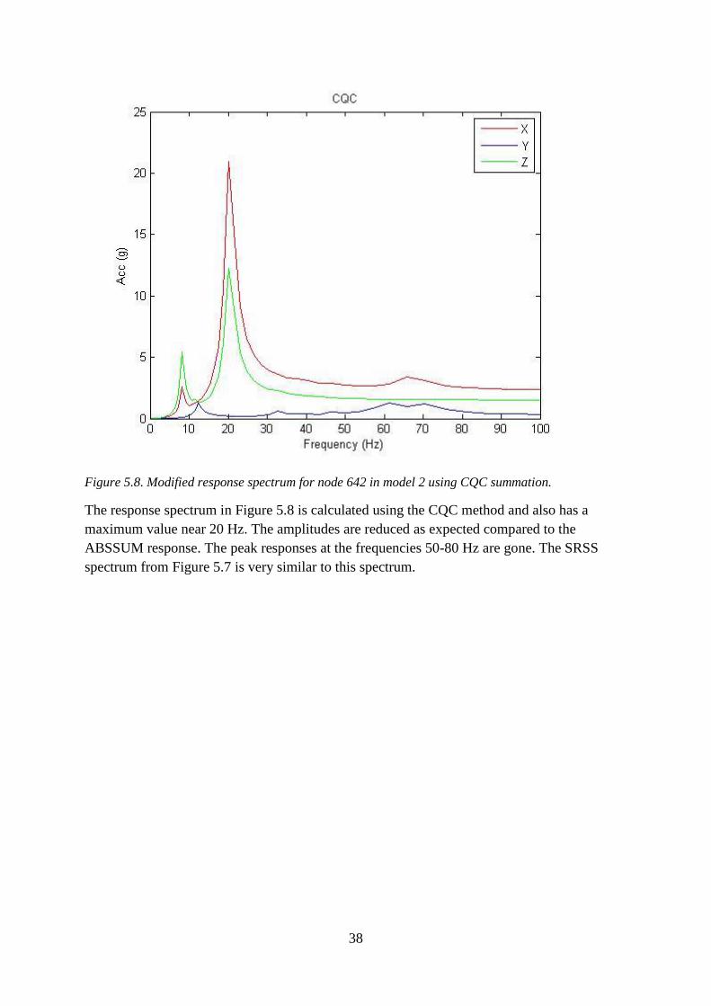
Figure 5.8. Modified response spectrum for node 642 in model 2 using CQC summation.

The response spectrum in Figure 5.8 is calculated using the CQC method and also has a

maximum value near 20 Hz. The amplitudes are reduced as expected compared to the

ABSSUM response. The peak responses at the frequencies 50-80 Hz are gone. The SRSS

spectrum from Figure 5.7 is very similar to this spectrum.

39

5.2.2 Modified response spectrum comparison

Figure 5.9. Modified response spectrum using the full modell (small bore pipe included) and CQC for

model 2.

To investigate the possible inertia effects of removing the small pipe from the system, the

modified response spectrum was also calculated for the full model 2. The response spectrum

is presented in Figure 5.9. Compared to Figure 5.8 there is basically no difference, and

removing the small pipe has no inertia effect on the large system.

5.2.3 Spring stiffness

The flexibility matrix, 𝑲−𝟏, was established by applying loads of 1 kN or 1 kNm in each

degree of freedom in the connection point.

𝑲−1 =

(

0.035 0 0.0370 0.048 0.001

0.372 0.001 0.094

0 −0.225 0.001−0.027 0 0.0380 −0.021 0

0 −0.027 0−0.225 0 −0.0210.001 0.038 0

0.024 0 −0.0260 0.023 0

−0.026 0 0.087 )

40

The approximate method gives the stiffnesses in Table 5.4.

Stiffnesses

Kx 28.58 kN/mm

Ky 20.69 kN/mm

Kz 10.61 kN/mm

Mx 42150 kNm/rad

My 44210 kNm/rad

Mz 11444 kNm/rad

Table 5.4. Approximate stiffness in anchor point for model 2

The natural frequencies of the small bore pipe with and without the stiffnesses are presented

in Table 5.5 below.

Natural frequncies (Hz) for model 2

Fixed anchor Spring stiffness

49.451 47.0066

51.074 47.5343

322.33 131.637

Table 5.5. Natural frequencies of the small bore pipe with and without spring stiffness for model 2.

The springs replace the completely rigid anchor point and reduce the natural frequencies of

the small bore pipe. This changes the maximum response for each mode since the response is

collected from the response spectrum for each natural frequency.

5.2.4 Summary Model 2

Presented in Table 5.6 is the ratio of calculated stress in the separated small pipe model

compared to calculated stress in the full model. If the ratio is 1 the modified response

spectrum caused the same stress in that node as the full model. Ratio > 1 means the modified

response spectrum produced conservative results, ratio < 1 non-conservative. Node 642 is the

connection point, 3070 is the last node.

The results in Table 5.6 show that the stresses in the small pipe are described well by the use

of the modified response spectrum. The stresses in the removed small pipe are lower near the

connection point, and near the end of the pipe the stresses are the same. The modified

response spectrum with the CQC method with spring stiffness at the anchor point give

stresses that are 92% - 101% of those calculated with the full model.

41

Model 2 – Summary of stress ratio in separated pipe

ABSSUM SRSS CQC

Node Fixed anchor Spring Fixed anchor Spring Fixed anchor Spring

642 0.76 0.83 0.89 0.89 0.89 0.92

3000 0.76 0.82 0.90 0.90 0.89 0.92

3010 0.75 0.80 0.90 0.91 0.89 0.93

3020 0.76 0.80 0.91 0.92 0.90 0.93

Z001 0.77 0.80 0.92 0.93 0.92 0.95

3030 0.79 0.82 0.95 0.95 0.94 0.97

3040 0.80 0.82 0.96 0.96 0.95 0.98

3050 0.88 0.88 1 0.99 0.99 1.01

3060 0.91 0.91 1 1 1 1

3070 1 1 1 1 1 1

Table 5.6. Ratio of stress in small bore pipe from model 1 nodes using the modified response spectrum

compared to the original response spectra.

42

6. Conclusions There is no experimental data to compare the results to at this time. This makes the modified

response spectrum hard to validate from a practical standpoint. The thesis only examines two

models using certain computer software and has a very limited scope. Still, the results from

the two models can be looked at in a number of ways from a theoretical and norm-based

standpoint.

It can be concluded that the method of a modified response spectrum does not provide

consistently conservative results if they are compared to ASME-accepted methods such as

modeling the complete system as one. The reason that conservatism is being considered is that

there is a desire for a simple method that allows for the parting of small bore pipes. If the

results are shown to be conservative, small pipes could be allowed to be removed and

analyzed separately using the modified response spectrum. However, conservative results

should perhaps not be expected. There is nothing in the approach that should lead to

theoretical conservatism. There are no safety factors or other approximations, only the

dynamic amplification factor which is merely the theoretical increase of response due to

coinciding loading- and natural frequencies. In practical use the peaks of the modified

response spectra would be broadened to achieve more conservatism.

The stresses in the separated pipe have been compared to the stresses in the same pipe in the

original large system. Recall that one of the reasons for removing small bore pipes is twin

modes, the effects of which are reduced when systems are downsized. With this in mind, the

modified response spectrum could (perhaps even should) lead to non-conservative results

when it is generated from a reduced model since the effects of twin modes are reduced.

However, this should not influence the results that calculate response with the CQC method.

In the first model, the stresses are conservative in some parts and non-conservative in other

parts of the small pipe. The modified response spectrum does not recreate the conditions that

the small pipe is being subjected to when still connected in an adequate way. This could

possibly, in part, have its origin in an approximation being made when the small pipe is

removed. An assumption is made that the inertia of the small pipe is insignificant. The inertia

of the small pipe is, however, affecting the system in this model, and this can be illustrated by

calculating the modified response spectrum before and after the small pipe is removed. If the

assumption is correct, the spectra should be identical. This is not the case as is seen in Section

5.1.2.

The second model is much larger in absolute size, but also relative to the removed pipe. The

assumption that the small pipe is not affecting the system is more accurate than in the first

model, and thus the spectra in Section 5.2.2 are the same. Both the model with the fixed

connection point and the spring connection point give interesting results that gives reason to

think that the modified response spectrum can recreate the conditions of the original system in

a satisfactory way.

Using spring stiffness in the anchor point of the small pipe does seem to represent the

connection point better, and in turn the results. It is reasonable to believe that a more realistic

43

model of the anchor point would lead to even better resemblance. A full matrix formulation of

the stiffness would likely yield even more similar results.

The results show that the method of a modified response spectrum can give non-conservative

results. However, the “worst” non-conservative node still accounted for 88 % of the stress

calculated with the small bore pipes left in the models. Even if the results are non-

conservative, the comparisons made in this thesis might not tell the whole story. The response

spectrum method is already making use of a lot of approximations and is accepted by ASME

since it is considered conservative. Although not conservative, the results generated by the

modified response spectrum could in fact be closer to the “true” response; true time-history or

experimental response.

44

7. Future research There are possible ways forward to theoretically validate the modified response spectrum

method as conservative compared to ASME regulations.

The peaks of the modified response spectra could be broadened to include more conservatism.

A response spectrum load corresponds to several time history loads, and there are many time

history loads applied on a system that gives the same response spectra reaction at the

supports. ASME states that if three independent time history loads can be derived from a

response spectrum and these are enveloped to ensure conservatism, it is permitted to adopt

this time history load as a replacement for the original response spectrum. A system can be

parted and the removed pipe is analyzed with the enveloped time history load. If the stresses

found in the small pipe loaded by the time history load are found to be less than those

generated by the modified response spectrum (generated from the same original response

spectrum), it is reasonable to think that the modified response spectrum can also be accepted

by ASME and other authorities on the matter.

If it cannot be proven conservative compared to methods currently accepted by ASME, the

effect on a system’s inertia by removing a pipe, and the subsequent effects on a modified

response spectrum and its caused response, could be examined. Perhaps the modified

response spectrum can give accepted and usable results if the inertia is not changed by a

certain fraction.

The modeling of the connection point could be studied further. Using spring stiffness in all 6

degrees of freedom improved the model, and it is reasonable to think that a full stiffness

matrix would improve the model even more. Also, the springs could be modeled on the

connection point in the large pipe as well, to include some effects of the small pipe.

45

References Antaki, G.A. (1995). Analytical Considerations in the Code Qualification of Piping Systems.

Aiken: Westinghouse Savannah River Company.

Carr, A. J. (1994). Dynamic Analysis of Structures. New Zealand National Society for

Earthquake Engineering, 27(2).

Chopra, A. K. (1995). Dynamics of Structures: theory and applications to earthquake

engineering. New Jersey: Prentiss Hall.

Clough, R. W., & Penzien, J. (1993). Dynamics of Structures. New York: McGraw-Hill.

Datta, T. K. (2010). Seismic Analysis of Structures. Singapore: John Wiley & Sons.

Der Kiureghian, A. (1981). A response spectrum method for random vibration analysis of

MDF system. Earthquake Engineering and Structural Dynamics, 9.

DST Computer Services S.A. (1985). PIPESTRESS: Theory Manual for PIPESTRESS and

asociated programs.

DST Computer Services S.A. (2012). PIPESTRESS User's Manual, Version 3.7.0.

Gupta, A. K. (1990). Response Spectrum Method in Seismic Analysis and Design of

Structures. Cambridge: Blackwell Scientific.

Houdart, R., Hennart, J., & Urbano, M. (1997). Advanced Twin Mode Rotation. 5th

International Conference on Nuclear Engineering. Nice: Tractebel Engineering.

Möller, M. (2007). Responsspektrametodens matematiska bakgrund. Helsingborg.

Rosenblueth, E., & Elorduy, J. (1969). Responses of Linear Systems to Certain Transient

Disturbances. 4th World Conference on Earthquake Engineering. Santiago.

Smith, P. R., & Van Laan, T. J. (1987). Piping and Pipe Support Systems. New York:

McGraw-Hill.

U.S. Nuclear Regulatory Commission. (1976). Rev. 1, Regulatory Guide 1.92: Combining

modal responses and spatial components in seismic response analysis. Washington

D.C.

Welding Research Council. (1984, December). Technical Position on Industry Practice.

Welding Research Council Bulletin 300.

46

Appendix A

Calculation results

Model 1

The first model analyzed is the one from Figure 4.1. There are two response spectra loads

acting on two different levels. The modified response spectrum is calculated and can be found

in Section 5. Table A.1 show the stress ratio in each node in the separated pipe.

Model 1 - ABSSUM comparison

Node

Pipe still in model

-Stress ratio

Separated pipe

- Stress ratio % of stress

220 0.275 0.365 1.328658

Z001 0.138 0.16 1.15942

Z001 0.138 0.16 1.15942

270 0.128 0.167 1.304688

270 0.261 0.341 1.306513

280 0.249 0.32 1.285141

280 0.122 0.157 1.286885

290 0.072 0.058 0.805556

290 0.146 0.117 0.80137

300 0.128 0.115 0.898438

300 0.063 0.056 0.888889

Z002 0.019 0.016 0.842105

Z002 0.019 0.016 0.842105

310 0 0 1

Table A.1

47

These are the results using absolute summation on both levels and modes, in the order L/M/I.

Model 1 - SRSS comparison

Node

Pipe still in model

-Stress ratio

Separated pipe

- Stress ratio % of stress

220 0.121 0.156 1.292471

Z001 0.049 0.06 1.22449

Z001 0.049 0.06 1.22449

270 0.051 0.067 1.313725

270 0.103 0.137 1.330097

280 0.097 0.14 1.443299

280 0.047 0.069 1.468085

290 0.022 0.018 0.818182

290 0.045 0.037 0.822222

300 0.042 0.032 0.761905

300 0.021 0.016 0.761905

Z002 0.006 0.005 0.833333

Z002 0.006 0.005 0.833333

310 0 0 1

Table A.2

Model 1 - CQC comparison

Node

Pipe still in model

-Stress ratio

Separated pipe

- Stress ratio % of stress

220 0.121 0.158 1.309041

Z001 0.049 0.06 1.22449

Z001 0.049 0.06 1.22449

270 0.051 0.068 1.333333

270 0.103 0.138 1.339806

280 0.097 0.141 1.453608

280 0.047 0.069 1.468085

290 0.022 0.018 0.818182

290 0.045 0.038 0.844444

300 0.042 0.032 0.761905

300 0.02 0.016 0.8

Z002 0.005 0.005 1

Z002 0.005 0.005 1

310 0 0 1

Table A.3

48

The stress ratios in the separated pipe with a spring stiffness anchor loaded with a modified

response spectrum are presented in Table A.4.

Model 1 – with spring support

ABSSUM SRSS CQC

Separated pipe

- Stress ratio

% of stress Separated pipe

- Stress ratio

% of stress Separated pipe

- Stress ratio

% of stress

0.389 1.416 0.173 1.433 0.174 1.442

0.154 1.116 0.058 1.184 0.058 1.184

0.154 1.116 0.058 1.184 0.058 1.184

0.19 1.484 0.081 1.588 0.082 1.608

0.388 1.487 0.166 1.612 0.167 1.621

0.365 1.466 0.167 1.722 0.169 1.742

0.179 1.467 0.082 1.745 0.083 1.766

0.065 0.903 0.02 0.909 0.020 0.909

0.133 0.911 0.04 0.889 0.040 0.889

0.132 1.031 0.037 0.881 0.037 0.881

0.065 1.032 0.018 0.857 0.018 0.900

0.019 1 0.005 0.833 0.005 1

0.019 1 0.005 0.833 0.005 1

0 1 0 1 0 1

Table A.4

49

Model 2

Model 2 (312) - ABSSUM comparison

Node

Pipe still in model

-Stress ratio

Separated pipe

- Stress ratio % of stress

642 0.168 0.128 0.761905

3000 0.159 0.121 0.761006

3000 0.159 0.121 0.761006

3010 0.53 0.4 0.754717

3010 0.53 0.4 0.754717

3020 0.517 0.391 0.756286

3020 0.517 0.391 0.756286

Z001 0.435 0.333 0.765517

Z001 0.435 0.333 0.765517

3030 0.343 0.271 0.790087

3030 0.343 0.271 0.790087

3040 0.327 0.26 0.795107

3050 0.223 0.196 0.878924

3060 0.161 0.146 0.906832

3060 0.161 0.146 0.906832

3070 0.084 0.084 1

Table A.5

Model 2 (312) – SRSS comparison

Node

Pipe still in model

-Stress ratio

Separated pipe

- Stress ratio % of stress

642 0.065 0.058 0.892308

3000 0.062 0.056 0.903226

3000 0.062 0.056 0.903226

3010 0.198 0.179 0.90404

3010 0.198 0.179 0.90404

3020 0.194 0.176 0.907216

3020 0.194 0.176 0.907216

Z001 0.168 0.155 0.922619

Z001 0.168 0.155 0.922619

3030 0.139 0.132 0.94964

3030 0.139 0.132 0.94964

3040 0.134 0.128 0.955224

3050 0.124 0.124 1

3060 0.106 0.106 1

3060 0.106 0.106 1

3070 0.084 0.084 1

Table A.6

50

Model 2 (312) - CQC comparison

Node

Pipe still in model

-Stress ratio

Separated pipe

- Stress ratio % of stress

642 0.064 0.057 0.890625

3000 0.061 0.054 0.885246

3000 0.061 0.054 0.885246

3010 0.196 0.175 0.892857

3010 0.196 0.175 0.892857

3020 0.192 0.172 0.895833

3020 0.192 0.172 0.895833

Z001 0.166 0.152 0.915663

Z001 0.166 0.152 0.915663

3030 0.137 0.129 0.941606

3030 0.137 0.129 0.941606

3040 0.132 0.125 0.94697

3050 0.123 0.122 0.99187

3060 0.106 0.105 0.990566

3060 0.106 0.105 0.990566

3070 0.084 0.084 1

Table A.7

51

The stress ratios in the separated pipe with a spring stiffness anchor loaded with a modified

response spectrum are presented in table A.8.

Model 2 – with spring support

ABSSUM SRSS CQC

Separated pipe

- Stress ratio

% of stress Separated pipe

- Stress ratio

% of stress Separated pipe

- Stress ratio

% of stress

0.139 0.83 0.058 0.89 0.059 0.92

0.130 0.82 0.056 0.90 0.056 0.92

0.130 0.82 0.056 0.90 0.056 0.92

0.425 0.80 0.181 0.91 0.183 0.93

0.425 0.80 0.181 0.91 0.183 0.93

0.414 0.80 0.178 0.92 0.179 0.93

0.414 0.80 0.178 0.92 0.179 0.93

0.348 0.80 0.156 0.93 0.157 0.95

0.348 0.80 0.156 0.93 0.157 0.95

0.281 0.82 0.132 0.95 0.133 0.97

0.281 0.82 0.132 0.95 0.133 0.97

0.269 0.82 0.128 0.96 0.129 0.98

0.197 0.88 0.123 0.99 0.124 1.01

0.146 0.91 0.106 1 0.106 1

0.146 0.91 0.106 1 0.106 1

0.084 1 0.084 1 0.084 1

Table A.8