Development of GPS Receiver Kalman Filter Algorithms for ...

UNCLASSIFIED

Development of GPS Receiver Kalman Filter

Algorithms for Stationary, Low-Dynamics, and

High-Dynamics Applications

Peter W. Sarunic 1

1 Cyber and Electronic Warfare DivisionDefence Science and Technology Group

DST-Group–TR–3260

ABSTRACT

This report presents algorithms that can be utilized in a GPS receiver to convert satellite-to-receiver pseudo-ranges to receiver position estimates. The report discusses a methodthat is used to determine instantaneous estimates of receiver position and then goes on todevelop three Kalman filter based estimators, which use stationary receiver, low dynamics,and high dynamics models for the receiver motion, respectively. These particular dynamicmodels are utilized because they are commonly used in actual GPS receivers, and covera wide range of applications. While the standard form of the Kalman filter, of which thethree filters just mentioned are examples, is theoretically correct, it can be susceptibleto numerical round-off errors, which can in some cases result in poor performance or, inthe worst case, filter divergence. This issue, and its solution, is investigated, and anotherversion of the high dynamics filter, which addresses this problem, is presented. Matlabcode was developed to test the performance of each of the filters and simulations wereperformed. The results of the simulations are also presented.

RELEASE LIMITATION

Approved for Public Release

UNCLASSIFIED

UNCLASSIFIED

Published by

Cyber and Electronic Warfare DivisionDefence Science and Technology GroupPO Box 1500Edinburgh, South Australia 5111, Australia

Telephone: 1300 333 362Facsimile: (08) 7389 6567

© Commonwealth of Australia 2016AR-016-601June, 2016

APPROVED FOR PUBLIC RELEASE

UNCLASSIFIED

UNCLASSIFIED

Development of GPS Receiver Kalman FilterAlgorithms for Stationary, Low-Dynamics, and

High-Dynamics Applications

Executive Summary

The Global Positioning system (GPS) is the primary source of information for a broadrange of positioning, navigation and timing systems. It is an all-weather, satellite-basedradio-navigation system which provides world-wide coverage. The objective of this reportis to present algorithms used in a central component of the system’s receiver positioncalculation, viz., to convert the satellite-to-receiver pseudo-ranges to receiver position es-timates. This report is one outcome of recent efforts to expand our knowledge base for thisimportant component of GPS receiver technology; this increased knowledge will facilitateour capabilities to provide scientifically based advice to the Australian Defence Force.

The report first describes a method for determining instantaneous estimates of receiverposition, and then goes on to develop three Kalman filter based receiver position estima-tors, i.e., a stationary receiver, low dynamics, and high dynamics estimator. As is impliedby their names, the three types of filters incorporate dynamic models that are optimizedfor situations where the receiver is stationary, is subjected to small accelerations, and tolarge accelerations, respectively. These estimators are designed to optimize performancefor commonly occurring applications, as is done in many GPS receivers.

The development of the three types of Kalman filter, as well as the instantaneous estimatoris presented in Section 2. Section 3 then presents the results of testing by simulation. Itis found that the simulations give indications of performance degradation, resulting fromerrors associated with numerical round-off, in the case of the high dynamics Kalman filter.This is then further investigated in Section 4 and an alternate form of the high dynamicsfilter is then developed to overcome the problem. The filter was implemented in Matlaband tested by simulation. The results of the simulations are also in Section 4. Finally,concluding remarks are presented in Section 5.

While this report deals specifically with GPS algorithms, the work covered forms partof a larger effort to develop algorithms for fusing GPS measurements with other sensordata, particularly measurements from inertial navigation systems (INS), to support R&Dinto multisensor positioning and navigation performance in non-benign environments. Thealgorithms presented in this report, and software developed for this work, will be requiredfor future research into deep integration of GPS with other sources of position data. Thesoftware will also be useful as a component of future modelling software that may need tobe developed for performance prediction of current or future systems that incorporate GPS.The ultimate aim is to help inform future capability requirements through the outcomesof this research.

UNCLASSIFIED

UNCLASSIFIED

THIS PAGE IS INTENTIONALLY BLANK

UNCLASSIFIED

UNCLASSIFIED

Author

Peter W. SarunicCEWD

Peter Sarunic was born in Adelaide, Australia, in 1958. Af-ter completing his B. Eng. degree in Electrical Engineering atthe University of Adelaide in 1980, he worked as an Electri-cal/Electronic Engineer in private industry for a period, andthen joined the Defence Science and Technology Organisationin 1986. His major areas of work were adaptive tracking, sig-nal processing, and radar systems engineering. In 1996, Pe-ter moved overseas to Canada, where he worked on radar anddata fusion problems. In 1998, he returned to DSTO, wherehe subsequently performed research on multipath track fusionfor over-the-horizon radar, multisensor fusion, electronic pro-tection for radar, and control and scheduling of UAVs. Whileemployed at DSTO, Peter completed a B.Sc. degree (mathe-matical and computer sciences), a M.Eng. degree (electronicengineering) and a PhD. degree (electronic engineering). Pe-ter’s current area of research is GPS/INS integration.

UNCLASSIFIED

UNCLASSIFIED


UNCLASSIFIED

UNCLASSIFIEDDST-Group–TR–3260

Contents

1 Introduction 1

2 Kalman Filter Development for the Processing of GPS measurements 2

2.1 Initial Single Point GPS solution . . . . . . . . . . . . . . . . . . . . . . . 2

2.2 Receiver Clock Bias Dynamic Model . . . . . . . . . . . . . . . . . . . . . 5

2.3 Plant and Measurement Equations for a Stationary Receiver . . . . . . . 5

2.4 Plant and Measurement Equations for a Low Dynamics Receiver . . . . . 7

2.5 Plant and Measurement Equations for a High Dynamics Receiver . . . . . 9

2.6 Extended Kalman Filter Equations - General Case . . . . . . . . . . . . . 10

2.7 Extended Kalman Filter Equations for a Stationary Receiver . . . . . . . 13

2.8 Extended Kalman Filter Equations for a Low Dynamics Receiver . . . . 15

2.9 Extended Kalman Filter Equations for a High Dynamics Receiver . . . . 16

3 Testing of Kalman Filter Algorithms 17

3.1 Kalman Filter with Stationary Receiver Model . . . . . . . . . . . . . . . 17

3.2 Kalman Filter with Low Dynamics Receiver Model . . . . . . . . . . . . . 20

3.3 Kalman Filter with High Dynamics Receiver Model . . . . . . . . . . . . 20

4 Minimizing Round-off Errors 25

4.1 Some Preliminaries . . . . . . . . . . . . . . . . . . . . . . . . . . . . . . . 28

4.2 Bierman-Thornton UD Filtering . . . . . . . . . . . . . . . . . . . . . . . 28

4.3 Testing of Bierman-Thornton UD Filter with High Dynamics ReceiverModel . . . . . . . . . . . . . . . . . . . . . . . . . . . . . . . . . . . . . . 31

4.4 Josephson Form Covariance Update . . . . . . . . . . . . . . . . . . . . . 34

5 Concluding Remarks 41

References 42

Appendices

A Matlab Code for Bierman Measurement Update 43

UNCLASSIFIED

DST-Group–TR–3260UNCLASSIFIED

Figures

1 Position estimation error of instantaneous estimates (stationary receiver model,300 updates). . . . . . . . . . . . . . . . . . . . . . . . . . . . . . . . . . . . . 18

2 Kalman filter position estimation error (300 updates), using stationary re-ceiver model. . . . . . . . . . . . . . . . . . . . . . . . . . . . . . . . . . . . . 18

3 Position estimation error of instantaneous estimates (stationary receiver model,3600 updates). . . . . . . . . . . . . . . . . . . . . . . . . . . . . . . . . . . . 19

4 Kalman filter position estimation error (3600 updates), using stationary re-ceiver model. . . . . . . . . . . . . . . . . . . . . . . . . . . . . . . . . . . . . 19

5 Position estimation error of instantaneous estimates (low dynamics receivermodel, 300 updates). . . . . . . . . . . . . . . . . . . . . . . . . . . . . . . . . 21

6 Kalman filter position estimation error (300 updates), using low dynamicsreceiver model. . . . . . . . . . . . . . . . . . . . . . . . . . . . . . . . . . . . 21

7 Position estimation error of instantaneous estimates (low dynamics receivermodel, 3600 updates). . . . . . . . . . . . . . . . . . . . . . . . . . . . . . . . 22

8 Kalman filter position estimation error (3600 updates), using low dynamicsreceiver model. . . . . . . . . . . . . . . . . . . . . . . . . . . . . . . . . . . . 22

9 Position estimation error of instantaneous estimates (high dynamics Kalmanfilter, 300 updates). . . . . . . . . . . . . . . . . . . . . . . . . . . . . . . . . . 23

10 Kalman filter position estimation error (300 updates), using high dynamicsreceiver model. . . . . . . . . . . . . . . . . . . . . . . . . . . . . . . . . . . . 24

11 Velocity estimates of high dynamics Kalman filter (300 updates). The red,green and blue plots are the x, y and z components of the velocity, respectively. 24

12 Acceleration estimates of high dynamics Kalman filter (300 updates). Thered, green and blue plots are the x, y and z components of the acceleration,respectively. . . . . . . . . . . . . . . . . . . . . . . . . . . . . . . . . . . . . . 25

13 Position estimation error of instantaneous estimates (high dynamics Kalmanfilter, 3600 updates). . . . . . . . . . . . . . . . . . . . . . . . . . . . . . . . . 26

14 Kalman filter position estimation error (3600 updates), using high dynamicsreceiver model. . . . . . . . . . . . . . . . . . . . . . . . . . . . . . . . . . . . 26

15 Velocity estimates of high dynamics Kalman filter (3600 updates). The red,green and blue plots are the x, y and z components of the velocity, respectively. 27

16 Acceleration estimates of high dynamics Kalman filter (3600 updates). Thered, green and blue plots are the x, y and z components of the acceleration,respectively. . . . . . . . . . . . . . . . . . . . . . . . . . . . . . . . . . . . . . 27

17 Position estimation error of instantaneous estimates (high dynamics Bierman-Thornton Kalman filter, 300 updates). . . . . . . . . . . . . . . . . . . . . . . 32

18 Bierman-Thornton Kalman filter position estimation error (300 updates), us-ing high dynamics receiver model. . . . . . . . . . . . . . . . . . . . . . . . . 32

UNCLASSIFIED


19 Velocity estimates of high dynamics Bierman-Thornton Kalman filter (300updates). The red, green and blue plots are the x, y and z components ofthe velocity, respectively. . . . . . . . . . . . . . . . . . . . . . . . . . . . . . . 33

20 Acceleration estimates of high dynamics Bierman-Thornton Kalman filter(300 updates). The red, green and blue plots are the x, y and z componentsof the acceleration, respectively. . . . . . . . . . . . . . . . . . . . . . . . . . . 33

21 Position estimation error of instantaneous estimates (high dynamics Bierman-Thornton Kalman filter, 3600 updates). . . . . . . . . . . . . . . . . . . . . . 34

22 Bierman-Thornton Kalman filter position estimation error (3600 updates),using high dynamics receiver model. . . . . . . . . . . . . . . . . . . . . . . . 35

23 Velocity estimates of high dynamics Bierman-Thornton Kalman filter (3600updates). The red, green and blue plots are the x, y and z components ofthe velocity, respectively. . . . . . . . . . . . . . . . . . . . . . . . . . . . . . . 35

24 Acceleration estimates of high dynamics Bierman-Thornton Kalman filter(3600 updates). The red, green and blue plots are the x, y and z componentsof the acceleration, respectively. . . . . . . . . . . . . . . . . . . . . . . . . . . 36

25 Position estimation error of instantaneous estimates (high dynamics Joseph-son Kalman filter, 300 updates). . . . . . . . . . . . . . . . . . . . . . . . . . 37

26 Josephson Kalman filter position estimation error (300 updates), using highdynamics receiver model. . . . . . . . . . . . . . . . . . . . . . . . . . . . . . 37

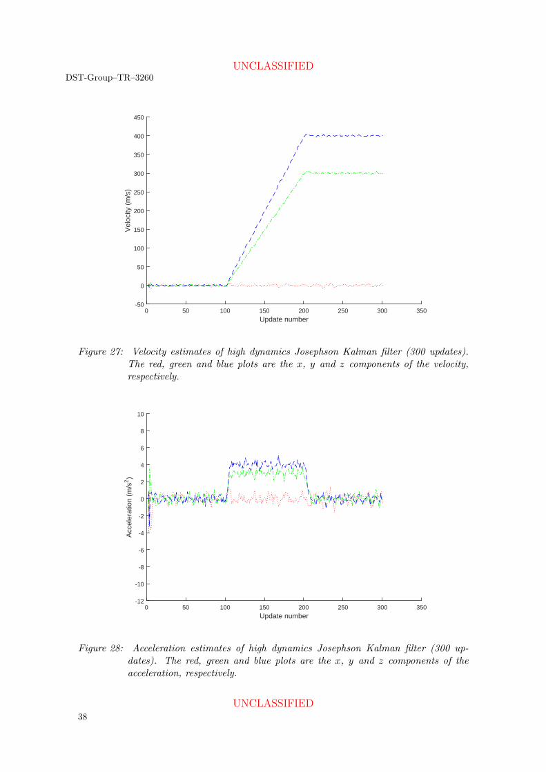
27 Velocity estimates of high dynamics Josephson Kalman filter (300 updates).The red, green and blue plots are the x, y and z components of the velocity,respectively. . . . . . . . . . . . . . . . . . . . . . . . . . . . . . . . . . . . . . 38

28 Acceleration estimates of high dynamics Josephson Kalman filter (300 up-dates). The red, green and blue plots are the x, y and z components of theacceleration, respectively. . . . . . . . . . . . . . . . . . . . . . . . . . . . . . 38

29 Position estimation error of instantaneous estimates (high dynamics Joseph-son Kalman filter, 3600 updates). . . . . . . . . . . . . . . . . . . . . . . . . . 39

30 Josephson Kalman filter position estimation error (3600 updates), using highdynamics receiver model. . . . . . . . . . . . . . . . . . . . . . . . . . . . . . 39

31 Velocity estimates of high dynamics Josephson Kalman filter (3600 updates).The red, green and blue plots are the x, y and z components of the velocity,respectively. . . . . . . . . . . . . . . . . . . . . . . . . . . . . . . . . . . . . . 40

32 Acceleration estimates of high dynamics Josephson Kalman filter (3600 up-dates). The red, green and blue plots are the x, y and z components of theacceleration, respectively. . . . . . . . . . . . . . . . . . . . . . . . . . . . . . 40

UNCLASSIFIED



UNCLASSIFIED


1 Introduction

The Global Positioning System (GPS) is a satellite-based radio-navigation system thatprovides world-wide, all-weather, coverage. GPS receivers decode and process messagesfrom in-view satellites to determine the receiver’s location as well as the current time; inthis report, GPS receiver position determination is considered. To determine the receiver’slocation, the GPS system uses time of arrival ranging. Each GPS receiver contains an in-ternal clock which it uses to determine the time of arrival of satellite ranging signals; usingthis information, the receiver calculates the time taken for the signal to travel from thesatellite to the receiver. Since the signal travels at the speed of light, c; this time intervalcan be converted to a distance by simply multiplying by c. The distance calculations arebiased by the receiver and satellite clock errors, and are therefore referred to as pseudo-ranges. Because of cost and other constraints, the receiver clock is in general much lessaccurate than the satellite clocks. If the location of four in-view satellites is known, andtheir ranges to the receiver are measured, the location of the receiver and its clock biascan be computed.

The objective of this report is to present the mathematics used to convert the satellite-to-receiver pseudoranges to receiver position estimates. The report discusses a method thatis used to determine instantaneous estimates of receiver position, i.e., estimates based onpseudo-ranges at one time instant, and then goes on to develop three Kalman filter basedestimators. Typically the instantaneous estimates are used to initialize a Kalman filter, asKalman filters require an initial estimate to start their recursions. The three Kalman filterestimators that are presented will be referred to as stationary receiver, low dynamics, andhigh dynamics filters. As is implied by their names, the three types of filters are optimizedfor situations where the receiver is stationary, is subjected to small accelerations, and tolarge accelerations, respectively. This approach is consistent with what can be found inmany actual GPS receivers, which allow the user to specify the dynamic level for the givenapplication.

While the standard form of the Kalman filter, of which the three filters just mentionedare examples, is theoretically correct, it can be susceptible to numerical round-off errors.The effects of these errors can be degraded filtering or, in some instances, Kalman filterinstability, leading to quite unpredictable behaviour. This issue, and its solution, is in-vestigated, and another version of the high dynamics filter is presented. Matlab code wasdeveloped to test the performance of each of the filters and simulations performed. Theresults of the simulations are also presented.

In Section 2, the development of the three types of Kalman filter, as well as the instanta-neous estimator is presented. Section 3 then presents the results of testing by simulation.It is noted that there are some indications of adverse effects due to numerical round-off inthe case of the high dynamics Kalman filter. To investigate this issue further, an alternateform of the high dynamics filter is developed in Section 4. The filter was implemented inMatlab and tested by simulation; the results of the simulations are also in Section 4. Atthe end of the paper, concluding remarks are presented in Section 5.

UNCLASSIFIED1


2 Kalman Filter Development for the Processing

of GPS measurements

2.1 Initial Single Point GPS solution

The GPS positioning problem has four unknowns that can be solved using the followingequations which use measurements from four satellites [1, p. 145].

ρ1 =[(X1 − x)2 + (Y1 − y)2 + (Z1 − z)2

]1/2+ ctr + χ1 (1)

ρ2 =[(X2 − x)2 + (Y2 − y)2 + (Z2 − z)2

]1/2+ ctr + χ2

ρ3 =[(X3 − x)2 + (Y3 − y)2 + (Z3 − z)2

]1/2+ ctr + χ3

ρ4 =[(X4 − x)2 + (Y4 − y)2 + (Z4 − z)2

]1/2+ ctr + χ4

where

χi = ctsvi + ctai + ei +mi + ηi, i = 1, .., 4

and ρi, i = 1, .., 4 are the measured pseudoranges from satellite i to the receiver an-tenna, Xi, Yi, Zi are the earth-centred-earth-fixed (ECEF) position coordinates of satellitei, x, y, z are the ECEF position coordinates of the receiver antenna, tr is the receiver clockbias, tsvi is the clock bias of satellite i, tai is the atmospheric delay, ei represents the errorin the broadcast ephemeris data, mi represents the multipath error, ηi represents receivertracking error noise, and c is the speed of light.

In equations 1, the pseudorange measurements are dependent on the receiver coordinatesin a nonlinear manner. While closed form solutions are available, typically the solution isfound by first linearizing the measurement equations, which can then be solved iteratively.The method described below relies on Newton’s method.

Let us assume that χi = 0, i = 1, .., 4, then the relationships between the pseudorangesand the receiver position are

ρ1 =[(X1 − x)2 + (Y1 − y)2 + (Z1 − z)2

]1/2+ ctr (2)

ρ2 =[(X2 − x)2 + (Y2 − y)2 + (Z2 − z)2

]1/2+ ctr

ρ3 =[(X3 − x)2 + (Y3 − y)2 + (Z3 − z)2

]1/2+ ctr

ρ4 =[(X4 − x)2 + (Y4 − y)2 + (Z4 − z)2

]1/2+ ctr

Note that in the above equation it is effectively assumed that the only source of rangebias is the receiver clock bias, which can be calculated and accounted for by solving foursimultaneous equations, instead of the minimum of three that would be required if therewas no range bias at all.

2

UNCLASSIFIED


Defining the vector x = (x, y, z, ctr) and linearizing Equations 2 results inρ1 (x)ρ2 (x)ρ3 (x)ρ4 (x)

=

ρ1 (x0)ρ2 (x0)ρ3 (x0)ρ4 (x0)

+ J

(x− x0)(y − y0)(z − z0)

(ctr − (ctr)0)

+ hot′s (3)

where x0 = (x0, y0, z0, (ctr)0) is the point of linearization, hot′s represents the higher orderterms in the expansion of Equations 2, and

J =

∂ρ1∂x

∂ρ1∂y

∂ρ1∂z

∂ρ1∂(ctr)

∂ρ2∂x

∂ρ2∂y

∂ρ2∂z

∂ρ2∂(ctr)

∂ρ3∂x

∂ρ3∂y

∂ρ3∂z

∂ρ3∂(ctr)

∂ρ4∂x

∂ρ4∂y

∂ρ4∂z

∂ρ4∂(ctr)

(x0,y0,z0,(ctr)0)

(4)

The partial derivatives in Equation 4 can easily be derived as

∂ρi∂x

=− (Xi − x)[

(Xi − x)2 + (Yi − y)2 + (Zi − z)2]1/2

(5)

∂ρi∂y

=− (Yi − y)[

(Xi − x)2 + (Yi − y)2 + (Zi − z)2]1/2

∂ρi∂z

=− (Zi − z)[

(Xi − x)2 + (Yi − y)2 + (Zi − z)2]1/2

∂ρi∂ (ctr)

= 1

Now, if we assume that hot′s = 0 in Equations 3, and χi = 0, i = 1, .., 4 in Equations 1,we can then form

ρ1 (x)ρ2 (x)ρ3 (x)ρ4 (x)

−ρ1

ρ2

ρ3

ρ4

=

ρ1 (x0)ρ2 (x0)ρ3 (x0)ρ4 (x0)

−ρ1

ρ2

ρ3

ρ4

+ J

(x− x0)(y − y0)(z − z0)

(ctr − (ctr)0)

=

0000

Let

% (x) =

ρ1 (x)ρ2 (x)ρ3 (x)ρ4 (x)

−ρ1

ρ2

ρ3

ρ4

then we have

UNCLASSIFIED3


% (x) = % (x0) + J

(x− x0)(y − y0)(z − z0)

(ctr − (ctr)0)

=

0000

Rearranging the above equation we have

% (x0) + J

xyzctr

− J

x0

y0

z0

(ctr)0

=

0000

Multiplying by J−1 gives

J−1% (x0) +

xyzctr

−

x0

y0

z0

(ctr)0

=

0000

and rearranging again gives

xyzctr

=

x0

y0

z0

(ctr)0

− J−1% (x0)

which is now in a suitable form for applying Newton’s method (also known as the Newton-

Raphson method) by just replacing x = (x, y, z, ctr) with xj+1 =(xj+1, yj+1, zj+1, (ctr)j+1

)and x0 = (x0, y0, z0, (ctr)0) with xj =

(xj , yj , zj , (ctr)j

), j = 0, 1, .., N resulting in

xj+1 = xj − J−1% (xj) (6)

We simply start with an initial guess for x0 = (x0, y0, z0, (ctr)0) and iterate till convergenceis reached. A simple test for convergence is ‖xj+1 − xj‖ < ε, where ε is set to a smallpositive value.

If measurements from more than four satellites are available, then J−1 in Equation 6 canbe replaced with

(JTJ

)−1JT to give the least squares solution, resulting in

xj+1 = xj −(JTJ

)−1JT% (xj) (7)

Equation 7 is referred to as the Gauss-Newton method. Note that Equation 7 assumesthat the pseudorange measurement errors have identical variances.

4

UNCLASSIFIED


2.2 Receiver Clock Bias Dynamic Model

One of the components of the Kalman filter models that are developed in this report isthe receiver clock bias model. The state space model used for the receiver clock bias isthat described on page 152 of [1]. The discrete time state transition equation is[

tr(k + 1)tr(k + 1)

]=

[1 T0 1

] [tr(k)tr(k)

]+

[ωdφ(k)ωdf (k)

]where T is the sampling period, and k is the time index.

The covariance matrix associated with the disctrete-time process noise vector[ωdφ(k) ωdf (k)

]Tis

Qdt (k) =

[SφT + T 3

3 SfT 2

2 SfT 2

2 Sf SfT

]

where Sφ and Sf are the power spectral densities of ωφ and ωf (the continuous-time processnoises) respectively. An example value of the discrete time process noise covariance matrix,scaled to metres, is shown on page 153 of [1]. It is

Qd (k) = c2Qdt (k) =

[0.0114 0.00190.0019 0.0039

](8)

2.3 Plant and Measurement Equations for a Stationary Re-ceiver

Before going further, a comment on notation is required. Many of the equations de-scribed in this report contain matrices and vectors whose elements are functions of time(represented by the time index k). To shorten the equations somewhat, a shorthandnotation is used where appropriate; viz., consider an m × n matrix A, with elementsaij (k) , i = 1, ..,m, j = 1, .., n, then

a11 . . . a1n

. . . . .

. . . . .

. . . . .am1 . . . amn

k

≡

a11 (k) . . . a1n (k). . . . .. . . . .. . . . .

am1 (k) . . . amn (k)

As can be found on page 105 of [1] (although full details are not given there), the discretetime state transition equation that is used for the stationary receiver case is

x (k + 1) = F (k) x (k) + v (k)

where

x (k)∆= [x, y, z, rtr , rtr ]

Tk , rtr (k)

∆= ctr (k) (9)

UNCLASSIFIED5


F (k) is the state transition matrix, v (k), k = 0, 1, ..., is a sequence of five dimensionalzero mean white Gaussian process noise, and

F (k) =

1 0 0 0 00 1 0 0 00 0 1 0 00 0 0 1 T0 0 0 0 1

(10)

The associated process noise covariance matrix (with the clock bias scaled to metres) thatis shown on page 105 of [1] as an example is

Qv (k) =

0 0 0 0 00 0 0 0 00 0 0 0 00 0 0 0.07 0.040 0 0 0.04 0.08

Note that the first three elements in the leading diagonal of the above matrix are zero;this is because the model assumes that the receiver is stationary.

The above covariance matrix is somewhat different to what would result from Equation8, i.e.:

Qv (k) =

0 0 0 0 00 0 0 0 00 0 0 0 00 0 0 0.0114 0.00190 0 0 0.0019 0.0039

(11)

This latter covariance matrix is used in the simulations. The most appropriate values forthe four bottom right hand elements of the matrix, of course, depend on the details of theparticular receiver that is being modelled.

It is convenient to write the measurement equation in component form. In this form it is

ρi (k + 1) =[(Xi (k + 1)− x (k + 1))2 + (Yi (k + 1)− y (k + 1))2 + (Zi (k + 1)− z (k + 1))2

]1/2

+rtr (k + 1)

for i = 1, .., Ns

Note that the measurement vector at time k is

ρ (k) =[ρ1 (k) ρ2 (k) . . ρNs (k)

]T(12)

For small increments in ∆x we can linearize as follows. Let ∆x (k + 1) = x (k + 1)−x (k),then in component form we can write

∆ρi (k + 1) = Hi (k + 1) ∆x (k + 1) + vi (k + 1)

or in vector form it is

∆ρ (k + 1) = H (k + 1) ∆x (k + 1) + v (k + 1)

6

UNCLASSIFIED


where

H (k + 1) =

∂ρ1∂x

∂ρ1∂y

∂ρ1∂z

∂ρ1∂rtr

0∂ρ2∂x

∂ρ2∂y

∂ρ2∂z

∂ρ2∂rtr

0

. . . . .

. . . . .∂ρNs∂x

∂ρNs∂y

∂ρNs∂z

∂ρNs∂rtr

0

k+1

(13)

is the 5×Ns dimensional measurement matrix, and Ns is the number of satellite-to-receiverpseudorange measurements at time k.

The partial derivatives in the above matrix are

∂ρi∂x

=− (Xi − x)[

(Xi − x)2 + (Yi − y)2 + (Zi − z)2]1/2

∂ρi∂y

=− (Yi − y)[

(Xi − x)2 + (Yi − y)2 + (Zi − z)2]1/2

∂ρi∂z

=− (Zi − z)[

(Xi − x)2 + (Yi − y)2 + (Zi − z)2]1/2

∂ρi∂rtr

= 1 where i = 1, .., Ns

The corresponding measurement noise covariance matrix is

R (k) =

σ2r1 0 . . 00 σ2

r2 . . 0. . . . .. . . . .0 0 . . σ2

rNs

k

(14)

where σ2ri (k) , i = 1, .., Ns is measurement noise variance for the measurement from satel-

lite i at time k.

2.4 Plant and Measurement Equations for a Low DynamicsReceiver

A short description of the continuous time low dynamics receiver model can be foundon page 243 of [1] (although full details are not given there). We need to use a discretetime model; a good approximation to the corresponding discrete time model is as follows[2, Section 6.3.2]. In this model the receiver’s acceleration is modelled using piecewiseconstant white acceleration noise. The discrete-time state transition equation is

x (k + 1) = F (k) x (k) + Γ (k) v (k)

UNCLASSIFIED7


where Γ (k) is noise gain at time k, x (k)∆= [x, x, y, y, z, z, rtr , rtr ]

Tk , rtr (k)

∆= ctr (k), and

F (k) =

1 T 0 0 0 0 0 00 1 0 0 0 0 0 00 0 1 T 0 0 0 00 0 0 1 0 0 0 00 0 0 0 1 T 0 00 0 0 0 0 1 0 00 0 0 0 0 0 1 T0 0 0 0 0 0 0 1

(15)

Γ (k) =

0.5T 2 0 0 0 0T 0 0 0 00 0.5T 2 0 0 00 T 0 0 00 0 0.5T 2 0 00 0 T 0 00 0 0 1 00 0 0 0 1

(16)

v (k) =[x y z cωdφ cωdf

]Tk

(17)

Let us now determine the process noise covariance matrix associated with this model. First

let us consider the covariance matrix associated with v (k), i.e., Qv (k) = E{

v (k) v (k)T}

.

We have

Qv (k) =

σ2x 0 0 0 0

0 σ2y 0 0 0

0 0 σ2z 0 0

0 0 0 σ2rφ

σrφσrf0 0 0 σrfσrφ σ2

rf

(18)

where σx, σy and σz are the standard deviations of the x, y, and z components of theacceleration noise, respectively, σrφ and σrf are the standard deviation of the clock biasprocess noise due to the phase error (scaled to metres), and that due to frequency error,respectively, and σrφσrf = σrfσrφ are their covariances. Note that the components of theacceleration noise are assumed to be independent of each other and the clock bias noises.

Now consider the process noise when multiplied by the gain matrix Γ (k), i.e., QΓv (k) =

E{

[Γ (k) v (k)] [Γ (k) v (k)]T}

. The resulting process noise covariance matrix can be shown

to be

QΓv (k) = Γ (k)Qv (k) Γ (k)T (19)

The measurement equation is the same as in Section 2.3, but with the measurement matrixnow being

8

UNCLASSIFIED


H (k + 1) =

∂ρ1∂x 0 ∂ρ1

∂y 0 ∂ρ1∂z 0 ∂ρ1

∂rtr0

∂ρ2∂x 0 ∂ρ2

∂y 0 ∂ρ2∂z 0 ∂ρ2

∂rtr0

. . . . . . . .

. . . . . . . .∂ρNs∂x 0

∂ρNs∂y 0

∂ρNs∂z 0

∂ρNs∂rtr

0

k+1

(20)

and the corresponding measurement noise covariance matrix is as in Equation 14.

2.5 Plant and Measurement Equations for a High DynamicsReceiver

A short description of the continuous time high dynamics receiver model can be found onpage 244 of [1] (although full details are not given there). We need to use a discrete timemodel; for this we will use the Wiener process acceleration model described in Section6.2.3 of [2]; this model is also sometimes called the white noise jerk model. Note that thisis a discretized continuous time model, as opposed to the direct discrete time model ofSection 6.3.3 of [2]. Which of these two models to use is a matter of choice; both are anapproximation to the actual continuous time dynamics of the receiver.

The discrete-time state transition equation is

x (k + 1) = F (k) x (k) + v (k)

where

x (k)∆= [x, x, x, y, y, y, z, z, z, rtr , rtr ]

Tk , rtr (k)

∆= ctr (k) (21)

and

F (k) =

1 T 12T

2 0 0 0 0 0 0 0 00 1 T 0 0 0 0 0 0 0 00 0 1 0 0 0 0 0 0 0 00 0 0 1 T 1

2T2 0 0 0 0 0

0 0 0 0 1 T 0 0 0 0 00 0 0 0 0 1 0 0 0 0 00 0 0 0 0 0 1 T 1

2T2 0 0

0 0 0 0 0 0 0 1 T 0 00 0 0 0 0 0 0 0 1 0 00 0 0 0 0 0 0 0 0 1 T0 0 0 0 0 0 0 0 0 0 1

(22)

With regard to the process noise model, let us first consider the x component for thecontinuous time system. The changes in acceleration are modelled by a continuous timezero-mean white noise as follows

...x (t) = vx (t)

Note that the acceleration is a Wiener process, and its derivative, the jerk, is representedby a white noise model. The changes in acceleration over a sampling period T are of

UNCLASSIFIED9


the order of√qxT , where qx is the power spectral density of the continuous time process

noise vx (t). The same can be done for the y and z components. Considering all threecomponents as well as the receiver clock error noise model of Section 2.2, we have the

following discrete time process noise covariance matrix (i.e., Qv (k)∆= E

{v (k) v (k)T

})

Qv (k) =

0 0 0 0 0 0 0 0Qx 0 0 0 0 0 0 0 0

0 0 0 0 0 0 0 00 0 0 0 0 0 0 00 0 0 Qy 0 0 0 0 00 0 0 0 0 0 0 00 0 0 0 0 0 0 00 0 0 0 0 0 Qz 0 00 0 0 0 0 0 0 00 0 0 0 0 0 0 0 0 σ2

rφσrφσrf

0 0 0 0 0 0 0 0 0 σrfσrφ σ2rf

(23)

where

Qx =

120T

5 18T

4 16T

3

18T

4 13T

3 12T

2

16T

3 12T

2 T

qxQy =

120T

5 18T

4 16T

3

18T

4 13T

3 12T

2

16T

3 12T

2 T

qyQz =

120T

5 18T

4 16T

3

18T

4 13T

3 12T

2

16T

3 12T

2 T

qzand qx, qy and qz are the power spectral densities of the x, y and z components of the con-tinuous time jerk noise, i.e., vx (t) , vy (t) and vt (t),respectively. Note that the componentsof the jerk noise are assumed to be independent of each other and the clock bias noises.

The measurement equation is the same as in Section 2.3, but with the measurement matrixnow being

H (k + 1) =

∂ρ1∂x 0 0 ∂ρ1

∂y 0 0 ∂ρ1∂z 0 0 ∂ρ1

∂rtr0

∂ρ2∂x 0 0 ∂ρ2

∂y 0 0 ∂ρ2∂z 0 0 ∂ρ2

∂rtr0

. . . . . . . . . . .

. . . . . . . . . . .∂ρNs∂x 0 0

∂ρNs∂y 0 0

∂ρNs∂z 0 0

∂ρNs∂rtr

0

k+1

(24)

and the corresponding measurement noise covariance matrix is as in Equation 14.

2.6 Extended Kalman Filter Equations - General Case

An extended Kalman filter [2, Section 10.3] is used as the estimation algorithm in thiswork. The algorithm is summarized in the sequel; before summarizing the algorithm, some

10

UNCLASSIFIED


definitions will first be given, as follows. Let

x (j|k)∆= E

[x (j) |Zk

]where

Zk∆= {z (j) , j ≤ k}

denotes the sequence of observations available at time k, and

E[x (j) |Zk

]is the conditional expectation of x (j) at time j given Zk.

If j = k, then x (j|k) is the estimate of the state (also called the filtered value); if j = k+1then x (j|k) is the predicted value (one-step) of the state. The state estimation error attime k is defined as

x (k|k)∆= x (k)− x (k|k)

The state prediction error at time k is defined as

x (k + 1|k)∆= x (k + 1)− x (k + 1|k)

The state estimation covariance matrix (i.e., the covariance associated with the estimatex (k|k) ) at time k is

P (k|k)∆= E

[x (k|k) x (k|k)T |Zk

]The state prediction covariance matrix (i.e., the covariance associated with the predictionx (k + 1|k) ) at time k is

P (k + 1|k)∆= E

[x (k + 1|k) x (k + 1|k)T |Zk

]The predicted measurement (one-step) is

z (k + 1|k)∆= E

[z (k + 1) |Zk

]The measurement prediction error (also called the innovation or residual) is defined as

ν (k + 1)∆= z (k + 1|k)

∆= z (k + 1)− z (k + 1|k)

The measurement prediction covariance matrix or innovation covariance matrix is

S (k + 1)∆= E

[z (k + 1|k) z (k + 1|k)T |Zk

]The Kalman filter gain is

W (k + 1)∆= P (k + 1|k)H (k + 1)T S (k + 1)−1

Now consider the nonlinear system with dynamics

x (k + 1) = f [k,x (k) ,u (k)] + v (k)

UNCLASSIFIED11


where x is the state vector, u is a known input, v is the process noise, which is assumedto be additive, zero mean, and white, and f is a vector-valued and possibly time varyingnon-linear function.

Let the measurement equation be

z (k) = h [k,x (k)] + w (k)

where w is the measurement noise, which is additive, zero mean, white, and uncorrelatedwith the process noise, and the function h is also vector valued and can be time varying.

The Extended Kalman filter is a suboptimal recursive algorithm for the above system, asfollows. First, we start with the initial estimate x (0|0) of x (0) and the associated initialcovariance P (0|0), both assumed to be available. Then, for estimation of the state of thesystem, starting with the state estimate x (k|k) at tk we have

State Prediction:

x (k + 1|k) = f [k, x (k|k) ,u (k)]

Measurement Prediction:

z (k + 1|k) = h [k + 1, x (k + 1|k)]

Measurement Residual:

ν (k + 1) = z (k + 1)− z (k + 1|k)

Updated State Estimate:

x (k + 1|k + 1) = x (k + 1|k) +W (k + 1)ν (k + 1)

For state covariance computation, starting with the state covariance P (k|k)at tk we have

Evaluation of Jacobians:

F (k) =∂f (k)

∂x

∣∣∣∣x=x(k|k)

H (k + 1) =∂h (k + 1)

∂x

∣∣∣∣x=x(k+1|k)

State Prediction Covariance:

P (k + 1|k) = F (k)P (k|k)F T (k) +Q (k)

Residual Covariance:

S (k + 1) = H (k + 1)P (k + 1|k)H (k + 1)T +R (k + 1)

Filter Gain:

W (k + 1) = P (k + 1|k)H (k + 1)T S (k + 1)−1

Updated State Covariance:

P (k + 1|k + 1) = P (k + 1|k)−W (k + 1)S (k + 1)W (k + 1)T

12

UNCLASSIFIED


2.7 Extended Kalman Filter Equations for a Stationary Re-ceiver

The extended Kalman filter for the stationary receiver case described in Section 2.3 willnow be described.

We start with the initial estimate x (0|0) of x (0) which is determined using the equationspresented in Section 2.1. Note that the initial estimate doesn’t give any information aboutthe rate of change of receiver clock bias - this needs to be guessed. Our initial guess isthat it’s zero. We also need to calculate the covariance, P (0|0) , of the initial estimatex (0|0), which can be determined as follows. Let PA be the covariance associated with theestimate of (x, y, z, ctr) obtained using Equation 7. Referring to Equation 4.11 in section4.1.1 of [1] we have

PA =(J (0)T R (0)−1 J (0)

)−1(25)

where

J (0) =

∂ρ1∂x

∂ρ1∂y

∂ρ1∂z

∂ρ1∂rtr

∂ρ2∂x

∂ρ2∂y

∂ρ2∂z

∂ρ2∂rtr

. . . .

. . . .∂ρNs∂x

∂ρNs∂y

∂ρNs∂z

∂ρNs∂rtr

∣∣∣∣∣∣∣∣∣∣∣x=x(0|0)

(26)

R (0) =

σ2r1 0 . . 00 σ2

r2 . . 0. . . . .. . . . .0 0 . . σ2

rNs

∣∣∣∣∣∣∣∣∣∣x=x(0|0)

(27)

Then

P (0|0) =

PA11 PA12 PA13 PA14 0PA21 PA22 PA23 PA24 0PA31 PA32 PA33 PA34 0PA41 PA42 PA43 PA44 0

0 0 0 0 2Qd22

Note that in the above matrix the covariances of the fifth column and fifth row can’t bedetermined from the measurements made on the initial startup, hence, as a reasonableguess, they are all set to zero, and the variance in the bottom right hand corner equalto 2Qd22 , i.e., twice the variance of element 22 of the discrete time receiver clock processnoise covariance matrix, scaled to metres, in Equation 8.

Then, for estimation of the state of the system, starting with the state estimate x (k|k) attk we have

State Prediction:

x (k + 1|k) = F (k) x (k|k) (28)

UNCLASSIFIED13


Measurement Prediction:

ρi (k + 1|k) =[(Xi (k + 1)− x (k + 1|k))2 + (Yi (k + 1)− y (k + 1|k))2 + (Zi (k + 1)− z (k + 1|k))2

]1/2

(29)

+ rtr (k + 1|k)

for i = 1, .., Ns

Measurement Residual:

ν (k + 1) = ρ (k + 1)− ρ (k + 1|k) (30)

Updated State Estimate:

x (k + 1|k + 1) = x (k + 1|k) +W (k + 1) ν (k + 1) (31)

For state covariance computation, starting with the state covariance P (k|k)at tk we have

Evaluation of Jacobians:

H (k + 1) =

∂ρ1∂x

∂ρ1∂y

∂ρ1∂z

∂ρ1∂rtr

0∂ρ2∂x

∂ρ2∂y

∂ρ2∂z

∂ρ2∂rtr

0

. . . . .

. . . . .∂ρNs∂x

∂ρNs∂y

∂ρNs∂z

∂ρNs∂rtr

0

∣∣∣∣∣∣∣∣∣∣∣x=x(k+1|k)

(32)

State Prediction Covariance:

P (k + 1|k) = F (k)P (k|k)F T (k) +QΓv (k) (33)

Residual Covariance:

S (k + 1) = H (k + 1)P (k + 1|k)H (k + 1)T +R (k + 1) (34)

Filter Gain:

W (k + 1) = P (k + 1|k)H (k + 1)T S (k + 1)−1 (35)

Updated State Covariance:

P (k + 1|k + 1) = P (k + 1|k)−W (k + 1)S (k + 1)W (k + 1)T (36)

where x (k), F (k), QΓv (k), ρ (k) and R (k) are defined in Equations 9, 10, 11, 12 and 14,respectively.

14

UNCLASSIFIED


2.8 Extended Kalman Filter Equations for a Low DynamicsReceiver

The extended Kalman filter for the low dynamics receiver case will now be described.

Again, we start with the initial estimate x (0|0) of x (0) which is determined using theequations presented in Section 2.1. Since the the initial estimate doesn’t give any infor-mation about the rate of change of receiver clock bias, this needs to be guessed. Our initialguess is that it’s zero. We also need to calculate the covariance, P (0|0) , of the initial es-timate x (0|0), which can be determined as follows. As in Section 2.7, Equation 25 is usedto determine PA, with J (0) and R (0) defined as in Equations 26 and 27, respectively.Note that PA is the covariance associated with the estimate of (x, y, z, ctr) obtained usingEquation 7.

Then

P (0|0) =

PA11 0 PA12 0 PA13 0 PA14 00 σ2

x (0) 0 0 0 0 0 0PA21 0 PA22 0 PA23 0 PA24 0

0 0 0 σ2y (0) 0 0 0 0

PA31 0 PA32 0 PA33 0 PA34 00 0 0 0 0 σ2

z (0) 0 0PA41 0 PA42 0 PA43 0 PA44 0

0 0 0 0 0 0 0 2Qd22

Note that in the above matrix the covariances (i.e., the off-diagonal terms) of the second,fourth, sixth and eight row as well as the second, fourth, sixth and eighth column can’tbe determined from the measurements made on the initial startup, hence, as a reasonableassumption, they are all set to zero. The variances of the x, y and z components of theinitial velocity estimate are assumed to be σ2

x (0) , σ2y (0) and σ2

z (0) respectively, and thebottom right hand element of P (0|0) is set to 2Qd22 , i.e., twice the variance of element22 of the discrete time receiver clock process noise covariance matrix, scaled to metres, inEquation 8.

Then for estimation of the state of the system, starting with the state estimate x (k|k) attk and for state covariance computation, starting with the state covariance P (k|k) at tkwe use Equations 28 to 31 and 33 to 36, where x (k), F (k), Γ (k), QΓv (k), ρ (k) and R (k)are defined in Equations 2.4, 15, 16, 19, 12 and 14, respectively and H (k + 1) is given by

H (k + 1) =

∂ρ1∂x 0 ∂ρ1

∂y 0 ∂ρ1∂z 0 ∂ρ1

∂rtr0

∂ρ2∂x 0 ∂ρ2

∂y 0 ∂ρ2∂z 0 ∂ρ2

∂rtr0

. . . . . . . .

. . . . . . . .∂ρNs∂x 0

∂ρNs∂y 0

∂ρNs∂z 0

∂ρNs∂rtr

0

∣∣∣∣∣∣∣∣∣∣∣x=x(k+1|k)

(37)

UNCLASSIFIED15


2.9 Extended Kalman Filter Equations for a High DynamicsReceiver

The extended Kalman filter for the high dynamics receiver case will now be described.Again, we start with the initial estimate x (0|0) of x (0) which is determined using theequations presented in Section 2.1. Since the the initial estimate doesn’t give any infor-mation about the rate of change of receiver clock bias, this needs to be guessed. Our initialguess is that it’s zero. We also need to calculate the covariance, P (0|0) , of the initial es-timate x (0|0), which can be determined as follows. As in Section 2.7, Equation 25 is usedto determine PA, with J (0) and R (0) defined as in Equations 26 and 27, respectively.Note that PA is the covariance associated with the estimate of (x, y, z, ctr) obtained usingEquation 7. Then

P (0|0) =

PA11 0 0 PA12 0 0 PA13 0 0 PA14 00 σ2

x (0) 0 0 0 0 0 0 0 0 00 0 σ2

x (0) 0 0 0 0 0 0 0 0PA21 0 0 PA22 0 0 PA23 0 0 PA24 0

0 0 0 0 σ2y (0) 0 0 0 0 0 0

0 0 0 0 0 σ2y (0) 0 0 0 0 0

PA31 0 0 PA32 0 0 PA33 0 0 PA34 00 0 0 0 0 0 0 σ2

z (0) 0 0 00 0 0 0 0 0 0 0 σ2

z (0) 0 0PA41 0 0 PA42 0 0 PA43 0 0 PA44 0

0 0 0 0 0 0 0 0 0 0 2Qd22

In the above matrix, the covariances (i.e., the off-diagonal terms) of the second, third,fifth, sixth, eight, ninth and eleventh row as well as the second, third, fifth, sixth, eight,ninth and eleventh column can’t be determined from the measurements made on the initialstartup, hence, as a reasonable assumption, they are all set to zero. The variances of thex, y and z components of the initial velocity estimate are assumed to be σ2

x (0) , σ2y (0) and

σ2z (0) respectively, the variances of the x, y and z components of the initial acceleration

estimate are assumed to be σ2x (0) , σ2

y (0) and σ2z (0) respectively, and the bottom right

hand element of P (0|0) is set to 2Qd22 , i.e., twice the variance of element 22 of the discretetime receiver clock process noise covariance matrix, scaled to metres, in Equation 8.

Then for estimation of the state of the system, starting with the state estimate x (k|k) attk and for state covariance computation, starting with the state covariance P (k|k) at tkwe use Equations 28 to 31 and 33 to 36, where x (k), F (k), Qv (k), ρ (k) and R (k) aredefined in Equations 21, 22, 23, 12 and 14, respectively and H (k + 1) is given by

H (k + 1) =

∂ρ1∂x 0 0 ∂ρ1

∂y 0 0 ∂ρ1∂z 0 0 ∂ρ1

∂rtr0

∂ρ2∂x 0 0 ∂ρ2

∂y 0 0 ∂ρ2∂z 0 0 ∂ρ2

∂rtr0

. . . . . . . . . . .

. . . . . . . . . . .∂ρNs∂x 0 0

∂ρNs∂y 0 0

∂ρNs∂z 0 0

∂ρNs∂rtr

0

∣∣∣∣∣∣∣∣∣∣∣x=x(k+1|k)

(38)

16

UNCLASSIFIED


3 Testing of Kalman Filter Algorithms

In order to test the algorithms developed in the previous sections, simulations were writtenusing the Matlab programming language. The aim of the simulations was to test theinstantaneous and Kalman filter estimators for stability and in general determine if theyare performing as expected. Simpifications were made in the scenarios considered, to theextent that was possible, while still achieving the aims of the testing. Modelling of therotation of the earth, and movement of the satellites was not required for this stage of thetesting and hence was not implemented in the simulations, i.e., it was assumed that thereceiver was in an arbitrary inertial reference frame and the satellites were stationary inthis frame, with a predefined geometric configuration relative to initial receiver position.The receiver-satellite geometry was made consistent with what could be expected for anactual situation. In the testing of the Kalman filter using a stationary receiver model,the receiver was kept stationary, whereas, for the other Kalman filters, the receiver wasin motion. Note that further testing with more sophisticated scenarios, utilizing actualsatellite trajectories would be desirable to fully test the filters which were developed.

3.1 Kalman Filter with Stationary Receiver Model

The Kalman filter using the stationary receiver model, which was described in Section2.7, was coded in Matlab and tested by simulation. The details of the simulations are asfollows.

The Kalman filter update rate was set to T = 1 sec. The number of updates that theKalman filter was run for was 300 to determine short term performance, and then 3600to determine performance over a longer period of time (1 hour). The latter served as amore extended test to determine if there are any issues associated with filter divergencedue to numerical round-off errors, which is a common problem in Kalman filter imple-mentations. The “actual” receiver range measurement error standard deviation was set toσra = 5m. The receiver range measurement error standard deviation as modelled by theKalman filter was set to σrm = 5m. Six satellites were modelled in the simulations; theirpositions were xs1 = (0.9390,−1.6265, 1.8781) × 107m, xs2 = (1.7648,−0.6423, 1.8781) ×107m, xs3 = (1.7648, 0.6423, 1.8781)× 107m, xs4 = (0.9390, 1.6265, 1.8781)× 107m, xs5 =(0.9390,−1.6265,−1.8781) × 107m, xs6 = (0.9390, 1.6265,−1.8781) × 107m. The receiverposition was xr =

(6.371× 106, 100, 150

)m.

Figures 1 and 2 show the results for the case of 300 updates. Figure 1 shows the errorsin the instantaneous position estimates; the instantaneous estimates were calculated usingthe Gauss-Newton method as described in Section 2.1. Figure 2 shows the errors inthe Kalman filter estimates. Note that the error is defined to be the distance betweenthe estimated position and the actual position. Looking at Figure 2, we see that theKalman filter is very quickly reducing the position estimate errors to well below that ofthe instantaneous estimates.

Figures 3 and 4 show the results for the case of 3600 updates; The primary reason fordoing the simulation that resulted in these figures was to test for divergence that mayresult from numerical round-off errors. As can be seen from the two figures, convergencecontinued for the duration of the simulation.

UNCLASSIFIED17


Update number0 50 100 150 200 250 300 350

Err

or (

met

res)

0

5

10

15

20

25

30

35

40

Figure 1: Position estimation error of instantaneous estimates (stationary receiver model,300 updates).

Update number0 50 100 150 200 250 300 350

Err

or (

met

res)

0

2

4

6

8

10

12

14

16

18

Figure 2: Kalman filter position estimation error (300 updates), using stationary receivermodel.

18

UNCLASSIFIED


Update number0 500 1000 1500 2000 2500 3000 3500 4000

Err

or (

met

res)

0

10

20

30

40

50

60

Figure 3: Position estimation error of instantaneous estimates (stationary receiver model,3600 updates).

Update number0 500 1000 1500 2000 2500 3000 3500 4000

Err

or (

met

res)

0

1

2

3

4

5

6

7

8

9

10

Figure 4: Kalman filter position estimation error (3600 updates), using stationary receivermodel.

UNCLASSIFIED19


3.2 Kalman Filter with Low Dynamics Receiver Model

The Kalman filter using the low dynamics receiver model, which was described in Section2.8, was coded in Matlab and tested by simulation. The details of the simulations are asfollows.

The Kalman filter update rate was set to T = 1 sec. The number of updates that theKalman filter was run for was 300 to determine short term performance, and then 3600to determine performance over a longer period of time (1 hour). The ”actual” receiverrange measurement error standard deviation was set to σra = 5m. The receiver rangemeasurement error standard deviation as modelled by the Kalman filter was set to σrm =5m. The (acceleration) process noise standard deviation in the Kalman filter was setto σx = σy = σz = 0.2 m/s2. Six satellites were modelled in the simulation; theirpositions were xs1 = (0.9390,−1.6265, 1.8781) × 107m, xs2 = (1.7648,−0.6423, 1.8781) ×107m, xs3 = (1.7648, 0.6423, 1.8781)× 107m, xs4 = (0.9390, 1.6265, 1.8781)× 107m, xs5 =(0.9390,−1.6265,−1.8781) × 107m, xs6 = (0.9390, 1.6265,−1.8781) × 107m. The initialreceiver position was xr =

(6.371× 106, 100, 150

)m; however, in these simulations the

receiver was not stationary, but instead had a velocity of vr = (0, 30, 40) m/s for theduration of the simulations.

Figures 5 and 6 show the results for the case of 300 updates. Figure 5 shows the errorsin the instantaneous position estimates. Figure 6 shows the errors in the Kalman filterestimates. Looking at Figure 6, we see that the Kalman filter is quickly reducing theposition estimate errors to below that of the instantaneous estimates. Note, however, thatthe errors in the position estimates are higher than was the case for the filter using thestationary receiver model. This is to be expected as this filter allows for receiver motion,and hence does not filter the position estimates as heavily. Of course, this filter has theadvantage that it can track the position and velocity of a moving receiver, whereas thefilter with the stationary receiver model is not designed for a moving receiver, and hencewould not be expected to function well for that case.

Figures 7 and 8 show the results for the case of 3600 updates. As can be seen from thetwo figures, convergence continued for the duration of the simulation.

3.3 Kalman Filter with High Dynamics Receiver Model

The Kalman filter using the high dynamics receiver model, which was described in Section2.9, was coded in Matlab and tested by simulation. The details of the simulations are asfollows.

The Kalman filter update rate was set to T = 1 sec. The number of updates thatthe Kalman filter was run for was 300 to determine short term performance, and then3600 to determine performance over a longer period of time (1 hour). The ”actual” re-ceiver range measurement error standard deviation was set to σra = 5m. The receiverrange measurement error standard deviation as modelled by the Kalman filter was setto σrm = 5m. The power spectral densities, qx, qy and qz, of the x, y and z compo-nents of the continuous time jerk noise were set to qx = qy = qz = 0.2. Six satelliteswere modelled in the simulation; their positions were xs1 = (0.9390,−1.6265, 1.8781) ×107m, xs2 = (1.7648,−0.6423, 1.8781) × 107m, xs3 = (1.7648, 0.6423, 1.8781) × 107m,

20

UNCLASSIFIED


Update number0 50 100 150 200 250 300 350

Err

or (

met

res)

0

5

10

15

20

25

30

35

40

45

50

Figure 5: Position estimation error of instantaneous estimates (low dynamics receivermodel, 300 updates).

Update number0 50 100 150 200 250 300 350

Err

or (

met

res)

0

2

4

6

8

10

12

14

16

18

Figure 6: Kalman filter position estimation error (300 updates), using low dynamics re-ceiver model.

UNCLASSIFIED21


Update number0 500 1000 1500 2000 2500 3000 3500 4000

Err

or (

met

res)

0

10

20

30

40

50

60

Figure 7: Position estimation error of instantaneous estimates (low dynamics receivermodel, 3600 updates).

Update number0 500 1000 1500 2000 2500 3000 3500 4000

Err

or (

met

res)

0

5

10

15

20

25

30

Figure 8: Kalman filter position estimation error (3600 updates), using low dynamicsreceiver model.

22

UNCLASSIFIED


Update number0 50 100 150 200 250 300 350

Err

or (

met

res)

0

5

10

15

20

25

30

35

40

45

50

Figure 9: Position estimation error of instantaneous estimates (high dynamics Kalmanfilter, 300 updates).

xs4 = (0.9390, 1.6265, 1.8781) × 107m, xs5 = (0.9390,−1.6265,−1.8781) × 107m, xs6 =(0.9390, 1.6265,−1.8781)×107m. The initial receiver position was xr =

(6.371× 106, 100, 150

)m.

The receiver was initially stationary, then, from t = 101 s to t = 200 s, it experienced anacceleration of ar = (0, 3, 4) m/s2.

Figures 9 and 10 show the results for the case of 300 updates. Figure 9 shows the errorsin the instantaneous position estimates. Figure 10 shows the errors in the Kalman filterestimates. Looking at Figure 10, we see that the Kalman filter is quickly reducing theposition estimate errors to below that of the instantaneous estimates; however, the errorsin the position estimates are higher than was the case for the filters using the stationaryreceiver and low dynamics models. Also, note that this filter has the advantage that itcan track the position, velocity and acceleration of the receiver. Figures 11 and 12 showthe velocity and acceleration estimates, respectively, for the case of 300 updates (samesimulation as that which produced Figures 9 and 10).

Figures 13 and 14 show the results for the case of 3600 updates. Figure 13 shows theerrors in the instantaneous position estimates, and Figure 14 shows the errors in theKalman filter estimates. Figures 15 and 16 show the velocity and acceleration estimates,respectively, for the case of 3600 updates (same simulation as that which produced Figures13 and 14). As can be seen from the two figures, convergence continued for the durationof the simulation. While, superficially, the performance of the high dynamics Kalmanfilter appears correct, a closer look indicates an anomoly. Looking at Figures 12 and 16,we note that the acceleration estimates are very heavily filtered subsequent to about 150updates. Noting the power spectral densities used in the Kalman filter model for the

UNCLASSIFIED23


Update number0 50 100 150 200 250 300 350

Err

or (

met

res)

0

5

10

15

20

25

Figure 10: Kalman filter position estimation error (300 updates), using high dynamicsreceiver model.

Update number0 50 100 150 200 250 300 350

Vel

ocity

(m

/s)

-50

0

50

100

150

200

250

300

350

400

450

Figure 11: Velocity estimates of high dynamics Kalman filter (300 updates). The red,green and blue plots are the x, y and z components of the velocity, respectively.

24

UNCLASSIFIED


Update number0 50 100 150 200 250 300 350

Acc

eler

atio

n (m

/s2)

-12

-10

-8

-6

-4

-2

0

2

4

6

8

10

Figure 12: Acceleration estimates of high dynamics Kalman filter (300 updates). Thered, green and blue plots are the x, y and z components of the acceleration,respectively.

continuous-time jerk noise, i.e., qx = qy = qz = 0.2, and referring to Equation 6.2.3-6 in[2], we would expect changes of acceleration during a sampling period T to be of the orderof√qxT ,

√qyT and

√qzT for the x, y and z components respectively, i.e.,

√0.2 ≈ 0.45

m/s2. Hence, given noisy measurements, we would intuitively expect that, after a periodof convergence, the acceleration estimates of the filter would exhibit acceleration noise ofthis order. Looking at Figures 12 and 16, we see that the acceleration noise is well belowthis, indicating that the filter is filtering more heavily than it is designed to do. A possiblecause of this is numerical roundoff error. This will be investigated in the following section.

4 Minimizing Round-off Errors

The Kalman filter implementations described up to this point will, from a theoreticalstandpoint, give correct results based on the models used; however, in practice they canbe somewhat sensitive to computer round-off errors. Round-off errors are a side effect ofcomputer arithmetic using a fixed number of bits for representing numbers. In this chapterwe will consider an alternative implementation technique that significantly reduces theeffects of these errors.

UNCLASSIFIED25


Update number0 500 1000 1500 2000 2500 3000 3500 4000

Err

or (

met

res)

0

5

10

15

20

25

30

35

40

45

50

Figure 13: Position estimation error of instantaneous estimates (high dynamics Kalmanfilter, 3600 updates).

Update number0 500 1000 1500 2000 2500 3000 3500 4000

Err

or (

met

res)

0

5

10

15

20

25

30

35

Figure 14: Kalman filter position estimation error (3600 updates), using high dynamicsreceiver model.

26

UNCLASSIFIED


Update number0 500 1000 1500 2000 2500 3000 3500 4000

Vel

ocity

(m

/s)

-50

0

50

100

150

200

250

300

350

400

450

Figure 15: Velocity estimates of high dynamics Kalman filter (3600 updates). The red,green and blue plots are the x, y and z components of the velocity, respectively.

Update number0 500 1000 1500 2000 2500 3000 3500 4000

Acc

eler

atio

n (m

/s2)

-12

-10

-8

-6

-4

-2

0

2

4

6

8

10

Figure 16: Acceleration estimates of high dynamics Kalman filter (3600 updates). Thered, green and blue plots are the x, y and z components of the acceleration,respectively.

UNCLASSIFIED27


4.1 Some Preliminaries

There have been various techniques developed as alternatives to the standard Kalmanfilter, with the aim of reducing the effects of round-off errors. A description of some ofthe most important techniques can be found in Chapter 6 of [3]. Amongst these, themost reliable and numerically stable implementations of the Kalman filter are collectivelyreferred to as square-root filters [3, Section 6.4]. Square-root filters use a reformulationof the state prediction and state estimate equations such that the dependent variable isa Cholesky factor, or modified Cholesky factor of the covariance matrices P (k + 1|k) andP (k + 1|k + 1). Two of the more favoured implementations of square-root filter are theCarlson-Schmidt square-root filter and the Bierman-Thornton UD filter. We will concen-trate on the Bierman-Thornton UD filter, as it, in particular, has been used successfullyon problems with thousands of state variables [3, p. 262].

First, let us summarize what Cholesky and modified Cholesky factors are [3, Section 6.4.3].The product of a matrix C with its own transpose in the form CCT = M is called thesymmetric product of C, and C is called a Cholesky factor of M . Note that, strictlyspeaking, a Cholesky factor is not a matrix square root, although the terms are oftenused interchangeably. All symmetric nonnegative definite matrices (of which covariancematrices are an example) have Cholesky factors. An upper triangular matrix U is calledunit upper triangular if its diagonal elements are all 1. Similarly, a lower triangularmatrix L is called unit lower triangular if all of its diagonal elements are 1. The modifiedCholesky decomposition of a symmetric positive definite matrix M is a decomposition intoproducts M = UDUT such that U is unit upper triangular and D is a diagonal matrix.This is also often called UD decomposition. The Bierman-Thornton UD filter relies onUD decomposition of the covariance matrices P (k + 1|k) and P (k + 1|k + 1) to achievesuperior numerical stability and robustness. The following section describes this filter.

4.2 Bierman-Thornton UD Filtering

For the sake of compactness, we now introduce the following subscript notation. Let Pk|k∆=

P (k|k), Pk+1|k∆= P (k + 1|k), and so on. Now, let Pk|k = Uk|kDk|kU

Tk|k, and Pk+1|k =

Uk+1|kDk+1|kUTk+1|k. Consider one cycle of the Kalman-filter covariance update now. The

state estimate error covariance matrix at time tk is Pk|k = Uk|kDk|kUTk|k. Consider first

the temporal update of the Kalman filter. The state prediction covariance for cycle k + 1is

Pk+1|k = FkPk|kFTk +Qk

Now, (from [3, Section 6.5.2.2]), let

A =

[UTk|kF

Tk

GTk

]

Dw =

[Dk|k 0

0 DQk

]and

Qk = GkDQkGTk

28

UNCLASSIFIED


where GkDQkGTk is the modified Cholesky decomposition of Qk. Then

ATDwA = FkUk|kDk|kUTk|kF

Tk +GkDQkG

Tk

= FkPk|kFTk +Qk

= Pk+1|k

= Uk+1|kDk+1|kUTk+1|k

Now, using the modified weighted Gram-Schmidt orthogonalization procedure ([3, p. 272])with respect to the diagonal weighting matrix Dw, we produce a unit lower triangular n×nmatrix L−1, a matrix B, and a diagonal matrix Dβ such that

A = BL

and

BTDwB = diag1≤i≤n {βi} = Dβ

hence

ATDwA = (BL)T DwBL

= LTBTDwBL

= LTDβL

Consequently, the factors

Uk+1|k = LT

Dk+1|k = Dβ

are the solutions of the (Thornton) temporal update problem for update k of the UDfilter. Note that the code that we used for implementing this was thornton.m as suppliedin soft-copy form with [3]. It was found in the directory Chapter 8.

Now, let us consider the measurement update. The updated state estimate covariance forcycle k is

Pk+1|k+1 = Pk+1|k − Pk+1|kHTk+1S

−1k+1Hk+1Pk+1|k

where

Sk+1 = Hk+1Pk+1|kHTk+1 +Rk+1

(Equations 2-229 and 2-224 of [4], respectively). Let us now consider the case where themeasurement update is a scalar. Then we have

Pk+1|k+1 = Pk+1|k − Pk+1|khk+1α−1k+1h

Tk+1Pk+1|k

where hk+1 is the vector corresponding to the row of Hk+1 that applies to the scalarmeasurement being considered,

αk+1 = hTk+1Pk+1|khk+1 + rk+1

UNCLASSIFIED29


and rk+1 is the variance of the measurement. Let Pk+1|k+1 = Uk+1|k+1Dk+1|k+1UTk+1|k+1

and Pk+1|k = Uk+1|kDk+1|kUTk+1|k, then we have

Uk+1|k+1Dk+1|k+1UTk+1|k+1 = Uk+1|kDk+1|kU

Tk+1|k

− Uk+1|kDk+1|kUTk+1|khk+1α

−1k+1h

Tk+1Uk+1|kDk+1|kU

Tk+1|k

= Uk+1|k

[Dk+1|k −Dk+1|kU

Tk+1|khk+1α

−1k+1h

Tk+1Uk+1|kDk+1|k

]UTk+1|k

Let v = Dk+1|kUTk+1|khk+1 then

Uk+1|k+1Dk+1|k+1UTk+1|k+1 = Uk+1|k

[Dk+1|k − vα−1

k+1vT]UTk+1|k

(note that Dk+1|k+1 = DTk+1|k+1 because Dk+1|k+1 is a diagonal matrix).

Now perform UD decomposition on (Dk+1|k − vα−1k+1v

T ) to get

Uk+1|k+1Dk+1|k+1UTk+1|k+1 = Uk+1|k

[UDUT

]UTk+1|k

=(Uk+1|kU

)D(Uk+1|kU

)Thence

Uk+1|k+1 = Uk+1|kU

Dk+1|k+1 = D

The algorithim for the UD decomposition of(Dk+1|k − vα−1

k+1vT)

to produce UDUT canbe found on page 78 of [5], and the corresponding Matlab code that was written to imple-ment the algorithm is listed in Appendix A.

Now, if the measurement is a vector, and the measurement covariance matrix is diagonal,then the scalar components of the measurement can simply be processed serially as scalarobservations with statistically independent measurement errors. This, in fact, is the casefor the measurements that we have. If the measurement covariance matrix is not diagonal,then the components cannot be processed serially; however, the measurement vector can beredefined, via a linear transformation, so that the measurement errors of its components areuncorrelated, i.e., the covariance matrix of the redefined measurement vector is diagonal.A procedure for doing this is described in Section 6.4.3.3 of [3].

Now, to start the Kalman filter, we need U0|0 and D0|0. To obtain these, we simply performUD decomposition on P0|0 as per Section 6.4.3.2 (Table 6.4) of [3]. UD decomposition isalso used in one other place in our simulation code, i.e., for computing PA as per Equation25. This is done as follows; we have

PA =(J (0)T R (0)−1 J (0)

)−1(39)

But R (0) = diag {ri (0)} is a diagonal matrix, so R (0)−1 = diag {1/ri (0)} and hence

computing(J (0)T R (0)−1 J (0)

)is computationally efficient and not very sensitive to

round-off errors. However, this is not the case when taking its inverse. Circumvention

30

UNCLASSIFIED


of this problem is done as follows. Let PI =(J (0)T R (0)−1 J (0)

)and now perform UD

decomposition on PI , resulting in PI = UIDIUTI , hence

PA =(UIDIU

TI

)−1

=(UTI)−1

D−1I U−1

I

=(U−1I

)TD−1I U−1

I

Hence, to obtain PA, we now only have to invert D, which is a diagonal matrix and Uwhich is a unit upper triangular matrix. This turns out to be less sensitive to numericalround-off errors than direct inversion of PI . The reader is referred to Section 6.4.3.5 andTables 6.4, 6.7 and 6.8 of [3] for a description of the MATLAB code for doing this. Notethat the functions that we used were SPDinv.m, UD decomp.m and UDinv.m, as suppliedin soft-copy form with [3]. They were found in the directory TABLE6pt8.

4.3 Testing of Bierman-Thornton UD Filter with High Dy-namics Receiver Model

The Bierman-Thornton implementation of the Kalman filter with the high dynamics re-ceiver model, as described in Section 4.2, was coded in Matlab and tested by simulation.These simulations and tests were done with the purpose of comparing the performancewith that of the standard form Kalman Filter (also using the high dynamics receivermodel). With the exception of now using the Bierman-Thornton implementation, allother parameters were kept identical to those used for the standard form Kalman Filtersimulations.

Figures 17, 18, 19 and 20 show the results for the case of 300 updates. Figure 17 showsthe errors in the instantaneous position estimates. Figure 18 shows the errors in theBierman-Thornton Kalman filter position estimates. Figures 19 and 20 show the velocityand acceleration estimates, respectively, for the case of 300 updates (same simulation asthat which produced Figures 17 and 18).

Comparing Figure 18 with Figure 10, we see that the filtered position estimate errors of theBierman-Thornton Filter appear to be similar to that of the standard form high dynamicsKalman filter. However, if we compare the velocity estimates in Figure 19 with that ofFigure 11, we note a considerable difference in performance. Comparing the accelerationestimates of Figure 20 with that of 12, we see an even greater difference in performance.

Figures 21, 22, 23 and 24 show the results for the case of 3600 updates. Figure 21 showsthe errors in the instantaneous position estimates. Figure 22 shows the errors in theBierman-Thornton Kalman filter estimates. Figures 23 and 24 show the velocity andacceleration estimates, respectively, for the case of 3600 updates (same simulation as thatwhich produced Figures 21 and 22). Comparing Figure 22 with Figure 14, we see thatthe filtered position estimate errors of the Bierman-Thornton Filter appear to be slightlysmaller than that of the standard form high dynamics Kalman filter. As was the casefor the 300 update simulations, when we compare the velocity estimates in Figure 23with that of Figure 15, we note a considerable difference in performance. Comparing the

UNCLASSIFIED31


Update number0 50 100 150 200 250 300 350

Err

or (

met

res)

0

5

10

15

20

25

30

35

40

45

50

Figure 17: Position estimation error of instantaneous estimates (high dynamics Bierman-Thornton Kalman filter, 300 updates).

Update number0 50 100 150 200 250 300 350

Err

or (

met

res)

0

5

10

15

20

25

Figure 18: Bierman-Thornton Kalman filter position estimation error (300 updates), us-ing high dynamics receiver model.

32

UNCLASSIFIED


Update number0 50 100 150 200 250 300 350

Vel

ocity

(m

/s)

-50

0

50

100

150

200

250

300

350

400

450

Figure 19: Velocity estimates of high dynamics Bierman-Thornton Kalman filter (300updates). The red, green and blue plots are the x, y and z components of thevelocity, respectively.

Update number0 50 100 150 200 250 300 350

Acc

eler

atio

n (m

/s2)

-12

-10

-8

-6

-4

-2

0

2

4

6

8

10

Figure 20: Acceleration estimates of high dynamics Bierman-Thornton Kalman filter (300updates). The red, green and blue plots are the x, y and z components of theacceleration, respectively.

UNCLASSIFIED33


Update number0 500 1000 1500 2000 2500 3000 3500 4000

Err

or (

met

res)

0

5

10

15

20

25

30

35

40

45

50

Figure 21: Position estimation error of instantaneous estimates (high dynamics Bierman-Thornton Kalman filter, 3600 updates).

acceleration estimates of Figure 24 with that of 16, we again see an even greater differencein performance.

Now looking at Figures 20 and 24, we note that the variations in the acceleration estimatesappear to be consistent with the acceleration noise used in the Kalman filter model, ascalculated at the end of Section 3.3. As further confirmation of this consistency, anotherrun of the simulation was performed for the case of 3600 updates, and the standarddeviation of the last 3000 acceleration estimates, for the x-component of acceleration, wascomputed, giving a result of approximately 0.41 m/s2, which is reasonably close to thevalue of 0.45 m/s2 that was calculated at the end of Section 3.3. Based on these results,indications are that the Bierman-Thornton filter is performing correctly, and the standardform Kalman filter, which was tested in Section 3.3, is not. To confirm this, a third formof the Kalman filter (i.e., the Josephson form), was implemented and simulations were runfor comparison with the standard form and Bierman-Thornton filters. This is describedin the following section.

4.4 Josephson Form Covariance Update

To confirm which of the two high dynamics filters is giving the correct estimates of thereceiver’s acceleration, the covariance update equation (Equation 36), as used in the stan-dard filter, was replaced with the Josephson form, which is considered to be less sensitiveto round-off errors. The Josephson form of the covariance update equation is as follows

34

UNCLASSIFIED


Update number0 500 1000 1500 2000 2500 3000 3500 4000

Err

or (

met

res)

0

5

10

15

20

25

30

35

Figure 22: Bierman-Thornton Kalman filter position estimation error (3600 updates),using high dynamics receiver model.

Update number0 500 1000 1500 2000 2500 3000 3500 4000

Vel

ocity

(m

/s)

-50

0

50

100

150

200

250

300

350

400

450

Figure 23: Velocity estimates of high dynamics Bierman-Thornton Kalman filter (3600updates). The red, green and blue plots are the x, y and z components of thevelocity, respectively.

UNCLASSIFIED35


Update number0 500 1000 1500 2000 2500 3000 3500 4000

Acc

eler

atio

n (m

/s2)

-12

-10

-8

-6

-4

-2

0

2

4

6

8

10

Figure 24: Acceleration estimates of high dynamics Bierman-Thornton Kalman filter(3600 updates). The red, green and blue plots are the x, y and z componentsof the acceleration, respectively.

[2, p. 294]

P (k + 1|k + 1) = [I −W (k + 1)H (k + 1)]P (k + 1|k) [I −W (k + 1)H (k + 1)]T

+ W (k + 1)R (k + 1)W (k + 1)T

The Kalman filter with the high dynamics receiver model, with the Josephson form re-placement, was coded in Matlab and tested by simulation. These simulations and testswere done with the purpose of comparing the performance with that of the standard formKalman Filter (also using the high dynamics receiver model), and the Bierman-Thorntonversion of the Kalman filter. All other parameters were kept identical to those used forthe standard form Kalman Filter and the Bierman-Thornton simulations.

Figures 25, 26, 27 and 28 show the results for the case of 300 updates. Figure 25 shows theerrors in the instantaneous position estimates. Figure 26 shows the errors in the JosephsonKalman filter estimates. Figures 27 and 28 show the velocity and acceleration estimates,respectively, for the case of 300 updates (same simulation as that which produced Figures25 and 26).

Figures 29, 30, 31 and 32 show the results for the case of 3600 updates. Figure 29 shows theerrors in the instantaneous position estimates. Figure 30 shows the errors in the JosephsonKalman filter estimates. Figures 31 and 32 show the velocity and acceleration estimates,respectively, for the case of 3600 updates (same simulation as that which produced Figures29 and 30).

36

UNCLASSIFIED


Update number0 50 100 150 200 250 300 350

Err

or (

met

res)

0

5

10

15

20

25

30

35

40

45

50

Figure 25: Position estimation error of instantaneous estimates (high dynamics Joseph-son Kalman filter, 300 updates).

Update number0 50 100 150 200 250 300 350

Err

or (

met

res)

0

5

10

15

20

25

Figure 26: Josephson Kalman filter position estimation error (300 updates), using highdynamics receiver model.

UNCLASSIFIED37


Update number0 50 100 150 200 250 300 350

Vel

ocity

(m

/s)

-50

0

50

100

150

200

250

300

350

400

450

Figure 27: Velocity estimates of high dynamics Josephson Kalman filter (300 updates).The red, green and blue plots are the x, y and z components of the velocity,respectively.

Update number0 50 100 150 200 250 300 350

Acc

eler

atio

n (m

/s2)

-12

-10

-8

-6

-4

-2

0

2

4

6

8

10

Figure 28: Acceleration estimates of high dynamics Josephson Kalman filter (300 up-dates). The red, green and blue plots are the x, y and z components of theacceleration, respectively.

38

UNCLASSIFIED


Update number0 500 1000 1500 2000 2500 3000 3500 4000

Err

or (

met

res)

0

5

10

15

20

25

30

35

40

45

50

Figure 29: Position estimation error of instantaneous estimates (high dynamics Joseph-son Kalman filter, 3600 updates).

Update number0 500 1000 1500 2000 2500 3000 3500 4000

Err

or (

met

res)

0

5

10

15

20

25

30

35

Figure 30: Josephson Kalman filter position estimation error (3600 updates), using highdynamics receiver model.

UNCLASSIFIED39


Update number0 500 1000 1500 2000 2500 3000 3500 4000

Vel

ocity

(m

/s)

-50

0

50

100

150

200

250

300

350

400

450

Figure 31: Velocity estimates of high dynamics Josephson Kalman filter (3600 updates).The red, green and blue plots are the x, y and z components of the velocity,respectively.

Update number0 500 1000 1500 2000 2500 3000 3500 4000

Acc

eler

atio

n (m

/s2)

-12

-10

-8

-6

-4

-2

0

2

4

6

8

10

Figure 32: Acceleration estimates of high dynamics Josephson Kalman filter (3600 up-dates). The red, green and blue plots are the x, y and z components of theacceleration, respectively.

40

UNCLASSIFIED


If we now compare the simulation results for Josephson form filter with the standard formfilter and the Bierman-Thornton UD filter we find the following.

Firstly, consider the simulations that were run for 300 updates. Comparing Figures 10,18 and 26, we note that the position estimation error appears to be approximately thesame for all three filters. Comparing Figures 11, 19 and 27, we see that the velocityestimates of Bierman-Thornton and Josephson filters are approximately the same. Thevelocity estimates of standard form filter are different, i.e, they are filtered more heavily.Comparing Figures 12, 20 and 28, we see that the acceleration estimates of Bierman-Thornton and Josephson filters are approximately the same. The acceleration estimatesof standard form filter are considerably different, i.e, they are filtered more heavily.

Now let us consider the simulations that were run for 3600 updates. Comparing Figures14, 22 and 30, we see that the position estimation error appears to be approximatelythe same for the Bierman-Thornton and Josephson filters. The position estimation errorfor the standard form filter appears to be slightly greater than for the other two filters.Comparing 15, 23 and 31, we find that the velocity estimates of Bierman-Thornton andJosephson filters are approximately the same. The velocity estimates of standard formfilter are different, i.e., they are filtered more heavily. Comparing Figures 16, 24 and32, we see that the acceleration estimates of Bierman-Thornton and Josephson filters areapproximately the same. The acceleration estimates of standard form filter are different,i.e., they are filtered more heavily.

In summary, the Bierman-Thornton and Josephson filters give approximately the same per-formance, whereas the standard form filter gives substantially different results, confirmingthat the standard form filter is performing incorrectly. Given that the only differencebetween the standard form and the Josephson form filter algorithms is the equation forthe state estimate covariance update, the result indicates that, for the simulations consid-ered, the primary cause of the incorrect behaviour of the standard form filter is the effectsof numerical error on the standard form state estimate covariance update equation i.e.,Equation 36.

5 Concluding Remarks

In this report, the mathematics used to convert GPS satellite-to-receiver pseudo-rangesto receiver position estimates is presented. First, the report discusses a method that isused to determine instantaneous estimates of receiver position; it then goes on to developthree Kalman filter based estimators. The three Kalman filter estimators use a stationaryreceiver, low dynamics, and high dynamics model for the receiver kinematics, respectively.The development of the three types of Kalman filter, as well as the instantaneous estimatoris presented in Section 2. Section 3 then presents the results of testing of the filters bysimulation. It is found that there are some indications of degraded performance due tonumerical round-off in the case of the high dynamics Kalman filter. To investigate thisissue further, an alternate form of the high dynamics filter, using modified Cholesky factorsof covariance matrices, is developed in Section 4. The filter was implemented in Matlaband tested by simulation. It is found that, for the simulations considered, the alternateform filter overcomes the problems associated with numerical errors. The results of the

UNCLASSIFIED41


simulations are also in Section 4.

References

1. Jay A. Farrell & Matthew Barth, The Global Positioning System & Inertial Navigation,McGraw-Hill, 1999.

2. Yaakov Bar-Shalom, Xiao-Rong Li, Estimation and Tracking: Principles, Techniques,and Software, Artech House, Inc., 1993.

3. Mohinder S. Grewal, Angus P. Andrews, Kalman Filtering Theory and Practice usingMATLAB, Third Edition, John Wiley and Sons, Inc., 2008.

4. Yaakov Bar-Shalom, Thomas E. Fortmann, Tracking and Data Association, AcademicPress, Inc., 1988.

5. Gerald J. Bierman, Factorization Methods for Discrete Sequential Estimation, Aca-demic Press, Inc., 1977.

42

UNCLASSIFIED


Appendix A Matlab Code for Bierman

Measurement Update

The following code was used in the implementation of the Bierman UD measurementupdate (cf., Section 4.2).

function [KalGain,U_post,D_post] = MyBierman(r,h,U_prior,D_prior)

%

% Matlab implementation of the Bierman "square root filtering without square roots",

% as interpreted from "Factorization Methods for Discrete Sequential Estimation",

% Gerard J. Bierman, 1977, Section V.3.

%

% P. W. Sarunic

%

% INPUTS:

% r variance of measurement error

% h measurement sensitivity (column) vector (note "h" is the same

% as the (column) vector "a" in Bierman’s book, Section V.3).

% U_prior unit upper triangular factor of covariance matrix of a priori state uncertainty

% D_prior diagonal factor of covariance matrix of a priori state uncertainty

%

% OUTPUTS:

% U_post upper triangular UD factor of a posteriori state uncertainty covariance

% D_post diagonal UD factor of a posteriori state uncertainty covariance

% KalGain Kalman filter gain

%

[VecLength, Unused] = size(U_prior);

f = U_prior’ * h;

v = D_prior * f;

alpha = zeros(VecLength,1);

alpha(1,1) = r + v(1,1)*f(1,1);

D_post = zeros(VecLength,VecLength);

D_post(1,1) = D_prior(1,1)*r/alpha(1,1);

K = zeros(VecLength,VecLength);

K(1,1) = v(1,1);

lambda = zeros(VecLength,1);

U_post = zeros(VecLength,VecLength);

U_post(:,1) = U_prior(:,1); % Note: I added this myself (it wasn’t expicitly

% mentioned in Bierman’s pseudo-code).

for j = 2:VecLength

alpha(j,1) = alpha(j-1,1) + v(j,1) * f(j,1);

D_post(j,j) = D_prior(j,j) * alpha(j-1,1)/alpha(j,1);

lambda(j,1) = -f(j,1)/alpha(j-1,1);

U_post(:,j) = U_prior(:,j) + lambda(j,1)*K(:,j-1);

K(:,j) = K(:,j-1) + v(j,1) * U_prior(:,j);

UNCLASSIFIED

43


end;

KalGain = K(:,VecLength)/alpha(VecLength,1);

44

UNCLASSIFIED

UNCLASSIFIED

DISTRIBUTION LIST

Development of GPS Receiver Kalman Filter Algorithms for Stationary, Low-Dynamics,and High-Dynamics Applications

Peter W. Sarunic

S&T Program

Chief of Cyber and Electronic Warfare Division 1

Research Leader, Systemic Protection and Effects 1

Head, PNT Technologies and Systems 1

Science Team Leader 1

Author 1

UNCLASSIFIED

UNCLASSIFIED

UNCLASSIFIED

Page classification: UNCLASSIFIED

DEFENCE SCIENCE AND TECHNOLOGY GROUPDOCUMENT CONTROL DATA

1. DLM/CAVEAT (OF DOCUMENT)

2. TITLE

Development of GPS Receiver Kalman Filter Algorithms

for Stationary, Low-Dynamics, and High-Dynamics Appli-

cations

3. SECURITY CLASSIFICATION (FOR UNCLASSIFIED RE-

PORTS THAT ARE LIMITED RELEASE USE (L) NEXT TO

DOCUMENT CLASSIFICATION)

Document (U)

Title (U)

Abstract (U)

4. AUTHOR

Peter W. Sarunic

5. CORPORATE AUTHOR

Defence Science and Technology Group

PO Box 1500

Edinburgh, South Australia 5111, Australia

6a. DST GROUP NUMBER

DST-Group–TR–3260

6b. AR NUMBER

016-601

6c. TYPE OF REPORT

Technical Report

7. DOCUMENT DATE

June, 2016

8. FILE NUMBER 9. TASK NUMBER 10. TASK SPONSOR 11. No. OF PAGES

44

12. No. OF REFS

5

13. DST Group Publications Repository

http://dspace.dsto.defence.gov.au/dspace/

14. RELEASE AUTHORITY

Chief, Cyber and Electronic Warfare Division

15. SECONDARY RELEASE STATEMENT OF THIS DOCUMENT

Approved for Public Release

OVERSEAS ENQUIRIES OUTSIDE STATED LIMITATIONS SHOULD BE REFERRED THROUGH DOCUMENT EXCHANGE, PO BOX 1500,EDINBURGH, SOUTH AUSTRALIA 5111

16. DELIBERATE ANNOUNCEMENT

No Limitations

17. CITATION IN OTHER DOCUMENTS

No Limitations

18. DST GROUP RESEARCH LIBRARY THESAURUS

Kalman filters, GPS, GNSS, Global Positioning System

19. ABSTRACT

This report presents algorithms that can be utilized in a GPS receiver to convert satellite-to-receiver pseudo-ranges to

receiver position estimates. The report discusses a method that is used to determine instantaneous estimates of receiver

position and then goes on to develop three Kalman filter based estimators, which use stationary receiver, low dynamics,

and high dynamics models for the receiver motion, respectively. These particular dynamic models are utilized because

they are commonly used in actual GPS receivers, and cover a wide range of applications. While the standard form of

the Kalman filter, of which the three filters just mentioned are examples, is theoretically correct, it can be susceptible to

numerical round-off errors, which can in some cases result in poor performance or, in the worst case, filter divergence.

This issue, and its solution, is investigated, and another version of the high dynamics filter, which addresses this problem,

is presented. Matlab code was developed to test the performance of each of the filters and simulations were performed.

The results of the simulations are also presented.

Page classification: UNCLASSIFIED

Development of GPS Receiver Kalman Filter Algorithms for ...

Documents

Transcript of Development of GPS Receiver Kalman Filter Algorithms for ...