Development of experimental techniques for …eprints.whiterose.ac.uk/83059/1/heat transfer rates...
37
This is a repository copy of Development of experimental techniques for measurement of heat transfer rates in heat exchangers in oscillatory flows. White Rose Research Online URL for this paper: http://eprints.whiterose.ac.uk/83059/ Version: Accepted Version Article: Kamsanam, W, Mao, X and Jaworski, AJ (2015) Development of experimental techniques for measurement of heat transfer rates in heat exchangers in oscillatory flows. Experimental Thermal and Fluid Science, 62. 202 - 215. ISSN 0894-1777 https://doi.org/10.1016/j.expthermflusci.2014.12.008 [email protected] https://eprints.whiterose.ac.uk/ Reuse Unless indicated otherwise, fulltext items are protected by copyright with all rights reserved. The copyright exception in section 29 of the Copyright, Designs and Patents Act 1988 allows the making of a single copy solely for the purpose of non-commercial research or private study within the limits of fair dealing. The publisher or other rights-holder may allow further reproduction and re-use of this version - refer to the White Rose Research Online record for this item. Where records identify the publisher as the copyright holder, users can verify any specific terms of use on the publisher’s website. Takedown If you consider content in White Rose Research Online to be in breach of UK law, please notify us by emailing [email protected] including the URL of the record and the reason for the withdrawal request.
Transcript of Development of experimental techniques for …eprints.whiterose.ac.uk/83059/1/heat transfer rates...
This is a repository copy of Development of experimental techniques for measurement of heat transfer rates in heat exchangers in oscillatory flows.
White Rose Research Online URL for this paper:http://eprints.whiterose.ac.uk/83059/
Version: Accepted Version
Article:
Kamsanam, W, Mao, X and Jaworski, AJ (2015) Development of experimental techniques for measurement of heat transfer rates in heat exchangers in oscillatory flows. Experimental Thermal and Fluid Science, 62. 202 - 215. ISSN 0894-1777
https://doi.org/10.1016/j.expthermflusci.2014.12.008
[email protected]://eprints.whiterose.ac.uk/
Reuse
Unless indicated otherwise, fulltext items are protected by copyright with all rights reserved. The copyright exception in section 29 of the Copyright, Designs and Patents Act 1988 allows the making of a single copy solely for the purpose of non-commercial research or private study within the limits of fair dealing. The publisher or other rights-holder may allow further reproduction and re-use of this version - refer to the White Rose Research Online record for this item. Where records identify the publisher as the copyright holder, users can verify any specific terms of use on the publisher’s website.
Takedown
If you consider content in White Rose Research Online to be in breach of UK law, please notify us by emailing [email protected] including the URL of the record and the reason for the withdrawal request.
1
Manuscript submitted to Experimental Thermal and Fluid Science
Development of experimental techniques for measurement of heat transfer rates
in heat exchangers in oscillatory flows
Wasan Kamsanam1, Xiaoan Mao2,* and Artur J. Jaworski2
1) Department of Engineering, University of Leicester, Leicester LE1 7RH, United Kingdom 2) Faculty of Engineering, University of Leeds, Leeds LS2 9JT, United Kingdom
Abstract
Heat exchangers are important components of thermoacoustic devices. In oscillatory flow
conditions, the flow and temperature fields around the heat exchangers can be quite complex, and
may significantly affect heat transfer behaviour. As a result, one cannot directly apply the heat
transfer correlations for steady flows to the design of heat exchangers for oscillatory flows. The
fundamental knowledge of heat transfer in oscillatory flows, however, is still not well-established.
The aim of the current work is to develop experimental apparatus and measurement techniques for
the study of heat transfer in oscillatory flows. The heat transferred between two heat exchangers
forming a couple was measured over a range of testing conditions. Three couples of finned-tube
heat exchangers with different fin spacing were selected for the experiment. The main parameters
considered were fin spacing, fin length, thermal penetration depth and gas displacement amplitude.
Their effects on the heat exchanger performance were studied. The results were summarised and
analysed in terms of heat transfer rate and dimensionless heat transfer coefficient: Colburn-j factor.
In order to obtain the gas side heat transfer coefficient in oscillatory flows, the water side heat
transfer coefficient is required. Thus, an experimental apparatus for unidirectional steady test was
also developed and a calculation method to evaluate the heat transfer coefficient was demonstrated.
The uncertainties associated with the measurement of heat transfer rate were also considered.
Keywords: Oscillatory flow; Heat exchanger; Heat transfer rate; Colburn-j factor;
Thermoacoustics
* To whom correspondence should be made Tel: +44(0) 113 343 4807, E-mail: [email protected] (X. Mao)
2
1. Introduction and literature review
In thermoacoustic heat engines, heat as an input energy is supplied from a high temperature source
through a hot heat exchanger and waste heat is rejected to a heat sink with low temperature. The
presence of the imposed steep temperature gradient in a solid structure called a stack or a
regenerator sandwiched between the two heat exchangers produces acoustic power. In
thermoacoustic refrigerators, heat is removed from where desired via a cold heat exchanger,
transported via a stack or regenerator by supplied acoustic power, and rejected to the heat sink in an
ambient heat exchanger. A simple standing wave thermoacoustic refrigerator and a schematic of
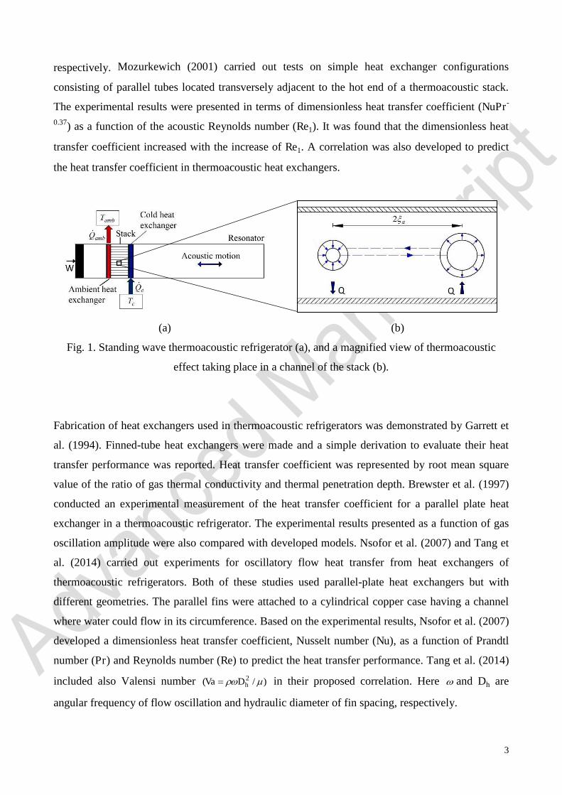
thermoacoustic effect are illustrated in Fig. 1. The main components in the device as shown in Fig.
1(a) are an acoustic driver, a stack and two heat exchangers placed in the resonator. The driver sets
up a half-wavelength acoustic field. This induces an oscillation of fluid elements in the vicinity of
the stack and the heat exchangers.
A thermodynamic process takes place as shown in Fig. 1(b) due to expansion and contraction of
fluid elements during their displacement cycle. The gas parcel at its largest volume moves leftward
while simultaneously experiencing compression. At the leftmost position, it rejects heat to the stack
as its temperature is raised above that of the local surface. This results in a decrease of the gas
parcel’s temperature which is subjected to the thermal contraction under high pressure. When the
parcel moves rightward, it experiences adiabatic expansion enlarging its volume and decreasing its
temperature below that of the local surface. At the rightmost position, the irreversible heat transfer
takes place from the stack plate to the gas parcel causing the expansion of gas parcel volume and
the rise of its temperature to the initial condition. All gas parcels behave as a ‘bucket brigade’
resulting in absorbing heat cQ at temperature Tc and rejecting heat ambQ at temperature Tamb. For a
standing wave thermoacoustic engine, the process can be described in similar manner as given
above for the refrigerator. However, the direction of thermodynamic cycle would be reversed.
As indicated, thermal interaction between working fluid and heat exchangers is crucial for the
performance of thermoacoustic devices. Experimental works have been carried out in order to study
the heat transfer in oscillatory flow. Temperature profiles at the interface of heated solid surface and
oscillating gas were observed by Bouvier et al. (2005). Surface heat flux was determined from the
temperature profiles measured on a test section of circular tube. The heat transfer characteristics
were analysed as a function of acoustic Reynolds number )/( 11 duRe . Here , , d and u1 are
density, dynamic viscosity of working gas, internal diameter of the tube and velocity amplitude,
3
respectively. Mozurkewich (2001) carried out tests on simple heat exchanger configurations
consisting of parallel tubes located transversely adjacent to the hot end of a thermoacoustic stack.
The experimental results were presented in terms of dimensionless heat transfer coefficient (NuPr-
0.37) as a function of the acoustic Reynolds number (Re1). It was found that the dimensionless heat
transfer coefficient increased with the increase of Re1. A correlation was also developed to predict
the heat transfer coefficient in thermoacoustic heat exchangers.
(a) (b)
Fig. 1. Standing wave thermoacoustic refrigerator (a), and a magnified view of thermoacoustic
effect taking place in a channel of the stack (b).
Fabrication of heat exchangers used in thermoacoustic refrigerators was demonstrated by Garrett et
al. (1994). Finned-tube heat exchangers were made and a simple derivation to evaluate their heat
transfer performance was reported. Heat transfer coefficient was represented by root mean square
value of the ratio of gas thermal conductivity and thermal penetration depth. Brewster et al. (1997)
conducted an experimental measurement of the heat transfer coefficient for a parallel plate heat
exchanger in a thermoacoustic refrigerator. The experimental results presented as a function of gas
oscillation amplitude were also compared with developed models. Nsofor et al. (2007) and Tang et
al. (2014) carried out experiments for oscillatory flow heat transfer from heat exchangers of
thermoacoustic refrigerators. Both of these studies used parallel-plate heat exchangers but with
different geometries. The parallel fins were attached to a cylindrical copper case having a channel
where water could flow in its circumference. Based on the experimental results, Nsofor et al. (2007)
developed a dimensionless heat transfer coefficient, Nusselt number (Nu), as a function of Prandtl
number (Pr) and Reynolds number (Re) to predict the heat transfer performance. Tang et al. (2014)
included also Valensi number )/( 2 hDVa in their proposed correlation. Here and Dh are
angular frequency of flow oscillation and hydraulic diameter of fin spacing, respectively.
4
Wakeland and Keolian (2004) carried out measurements of heat transfer between two identical
parallel plate heat exchangers (similar to car radiator) at various frequencies and gas displacement
amplitudes. From the results, a correlation was proposed in the form of heat transfer effectiveness
(the ratio of actual heat transfer rate to the maximum available heat transfer rate). A heat exchanger
of a similar type was employed in an experiment by Paek et al. (2005) to evaluate oscillating flow
heat transfer coefficient and to propose calculation methods. The experimental results were
compared with existing models and a new correlation was presented.
The design of heat exchangers is a critical task in thermoacoustics, yet the knowledge of heat
transfer in oscillatory flow conditions is limited. The relationship between heat transfer and heat
exchanger geometry, as well as the operating conditions, needs to be investigated. In order to
achieve the purpose, this study presents the development of an experimental apparatus in addition to
the techniques to determine the heat transfer performance of heat exchangers in oscillatory flows.
The dependence of the heat transfer rate and the dimensionless heat transfer coefficient, Colburn-j
factor, on normalized displacement amplitude and normalized fin spacing for the heat exchangers
under investigation is presented.
2. Experimental apparatus
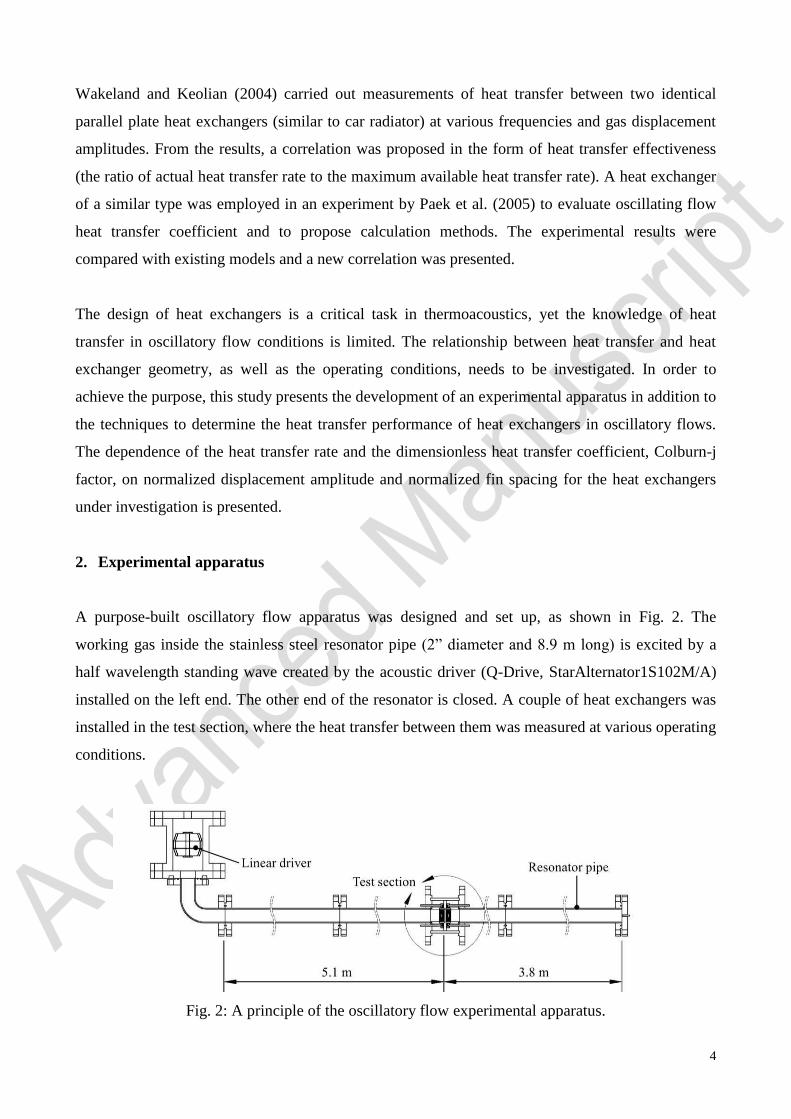
A purpose-built oscillatory flow apparatus was designed and set up, as shown in Fig. 2. The
working gas inside the stainless steel resonator pipe (2” diameter and 8.9 m long) is excited by a
half wavelength standing wave created by the acoustic driver (Q-Drive, StarAlternator1S102M/A)
installed on the left end. The other end of the resonator is closed. A couple of heat exchangers was
installed in the test section, where the heat transfer between them was measured at various operating
conditions.
Fig. 2: A principle of the oscillatory flow experimental apparatus.
5
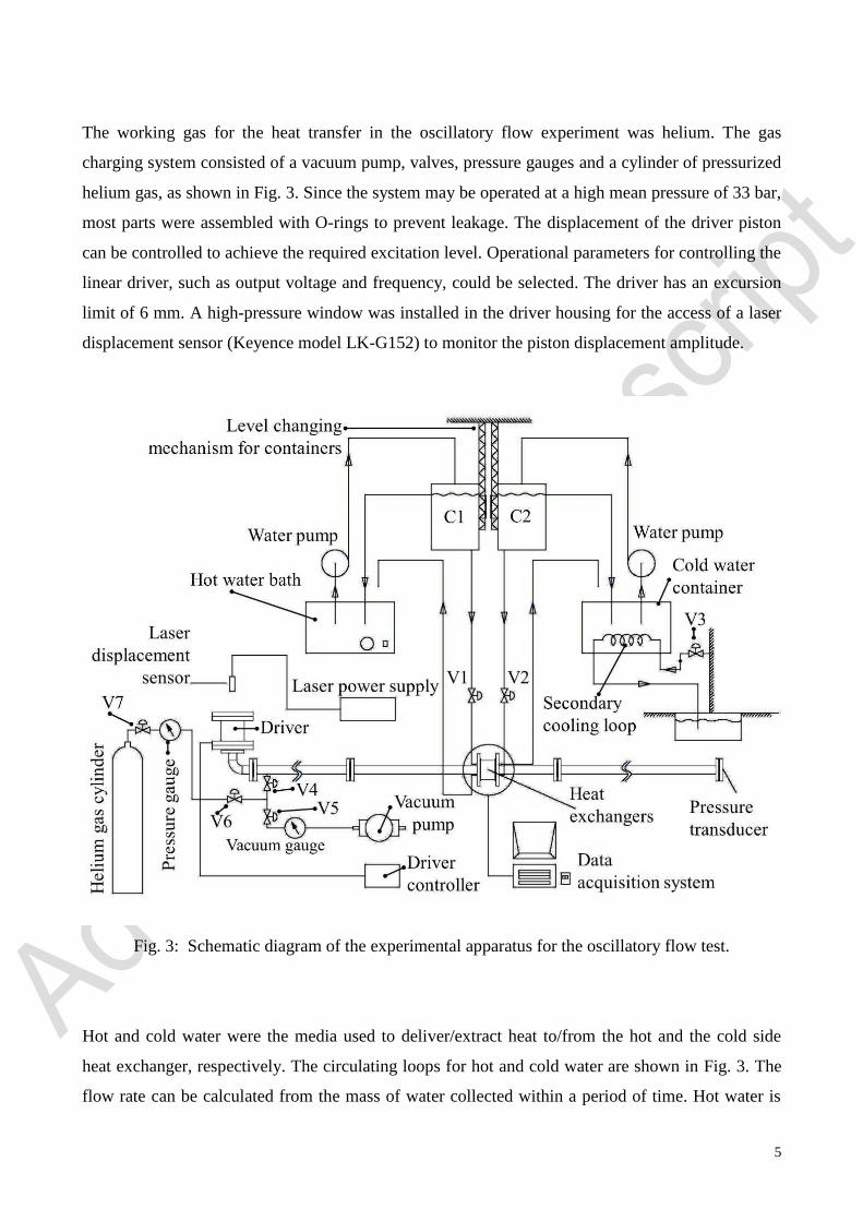
The working gas for the heat transfer in the oscillatory flow experiment was helium. The gas
charging system consisted of a vacuum pump, valves, pressure gauges and a cylinder of pressurized
helium gas, as shown in Fig. 3. Since the system may be operated at a high mean pressure of 33 bar,
most parts were assembled with O-rings to prevent leakage. The displacement of the driver piston
can be controlled to achieve the required excitation level. Operational parameters for controlling the
linear driver, such as output voltage and frequency, could be selected. The driver has an excursion
limit of 6 mm. A high-pressure window was installed in the driver housing for the access of a laser
displacement sensor (Keyence model LK-G152) to monitor the piston displacement amplitude.
Hot and cold water were the media used to deliver/extract heat to/from the hot and the cold side
heat exchanger, respectively. The circulating loops for hot and cold water are shown in Fig. 3. The
flow rate can be calculated from the mass of water collected within a period of time. Hot water is
Fig. 3: Schematic diagram of the experimental apparatus for the oscillatory flow test.
6
pumped from the hot water bath with a maximum heating power of 1500 W and circulated through
the hot heat exchanger. The water flow loop for the cold side heat exchanger was set up similar to
the one on the hot side. The mass flow rate for hot and cold heat exchanger can be controlled
through valves V1 and V2, respectively, or by changing the height of water containers. The
temperature of the cooling water measured at the inlet of the cold side heat exchanger was
maintained at 22 °C throughout the whole experiment. The secondary cooling flow loop was
installed in the cold water bath to keep the water temperature steady. In the secondary cooling loop,
cold water from a utility tap ran through a copper coil tube immersed in the cold water bath to carry
heat to an external heat sink. The temperature in the cold-water bath was controlled by adjusting the
flow rate of the cold water from the utility tap via valve V3 (see Fig. 3).
2.1 Test section
In the test section, two heat exchangers, one hot and another cold, were placed side by side. The
stack or the regenerator normally found in a typical thermoacoustic engine or refrigerator was not
present. This arrangement makes it possible to investigate the heat transfer from a heat exchanger to
the oscillatory flow in a relatively wide range of flow conditions, without the concern of the
operating mode of a thermoacoustic device being an engine or a refrigerator. The heat transfer
analysis is carried out using the calorimetric method by measuring the heat transfer rate on the hot
side heat exchanger, while the cold side heat exchanger is used to reject heat to the environment.
The investigated combinations of hot and cold heat exchangers, as A, B and C, are shown in Table
1, where individual heat exchangers are labelled by HEX-n, ‘n’ being the heat exchanger number.
The specification of heat exchangers is given in Section 2.2. A ceramic spacer was placed between
them to provide a 5 mm distance (gap) between the heat exchanger faces. One heat exchanger
performs as a hot heat exchanger and another as a cold heat exchanger. Heat transfer between them
is measured and the influence of relevant parameters on the heat transfer is analysed. The test
section is illustrated in Fig. 4.
Table 1: Hot and cold heat exchangers combinations
Combination Fin spacing, D
Hot heat exchanger Cold heat exchanger
A HEX-1, D = 0.7 mm HEX-1, D = 0.7 mm
B HEX-2, D = 1.4 mm HEX-3, D = 2.1 mm
C HEX-3, D = 2.1 mm HEX-2, D = 1.4 mm
7
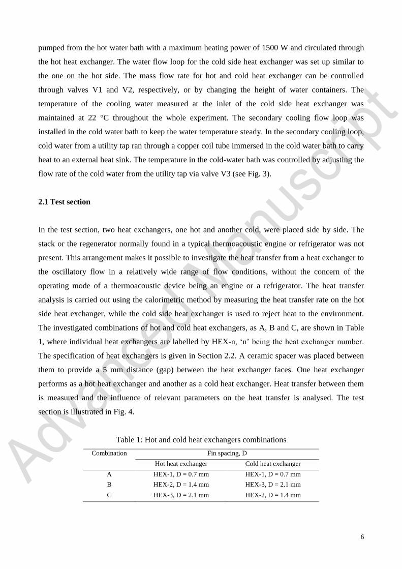
In order to minimize heat loss to the outside, insulation was applied where possible. Silicate wool
with a thermal conductivity of 0.1 W.m-1.K-1 was placed in the empty space between the heat
exchanger and the stainless steel housing. The internal surfaces of the stainless steel pipe on both
sides of the test section were covered by a polyethylene (PE) sheet with thermal conductivity of 0.5
W.m-1.K-1. The thickness of the PE sheet was 1.0 mm, which does not cause a significant
obstruction to the gas flow. The length of the PE sheet measured from the flange surface into the
pipe was about 10 cm; much longer than the maximum gas displacement amplitude in the
experiment. A ceramic plate with thermal conductivity of 1.46 W.m-1.K-1 was used to separate two
heat exchangers. It was introduced to reduce the heat conduction between hot and cold heat
exchangers. Each heat exchanger was separated from the test section end-flanges using PTFE
spacers – there is no direct contact between the copper heat exchanger case and the stainless steel
flange. The thermal conductivity of the PTFE spacer is 0.25 W.m-1.K-1.
2.2 Heat exchangers
The experiments were performed on heat exchangers with different fin spacings. The finned-tube
type heat exchanger was selected for this study due to the simplicity of its construction, which in
turn lowers the cost of fabrication. Heat exchanger specifications are detailed in Table 2. A
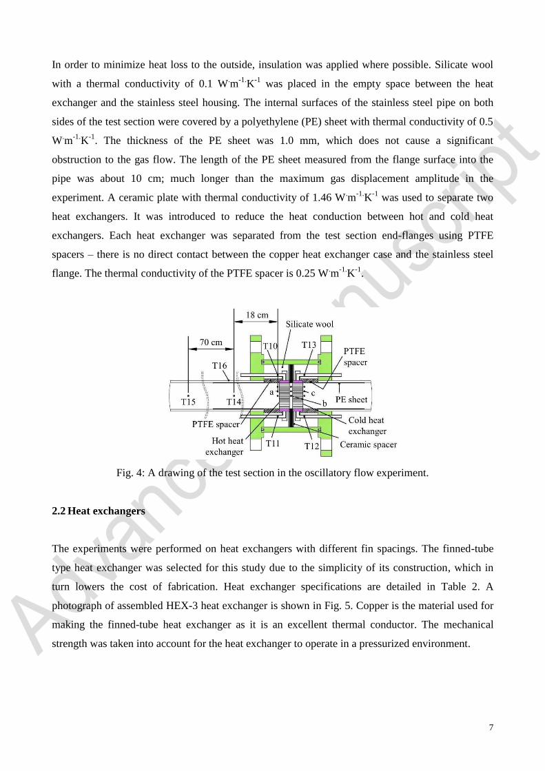
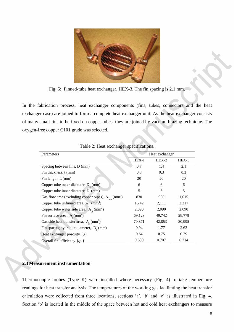
photograph of assembled HEX-3 heat exchanger is shown in Fig. 5. Copper is the material used for
making the finned-tube heat exchanger as it is an excellent thermal conductor. The mechanical
strength was taken into account for the heat exchanger to operate in a pressurized environment.
Fig. 4: A drawing of the test section in the oscillatory flow experiment.
8
In the fabrication process, heat exchanger components (fins, tubes, connectors and the heat
exchanger case) are joined to form a complete heat exchanger unit. As the heat exchanger consists
of many small fins to be fixed on copper tubes, they are joined by vacuum brazing technique. The
oxygen-free copper C101 grade was selected.
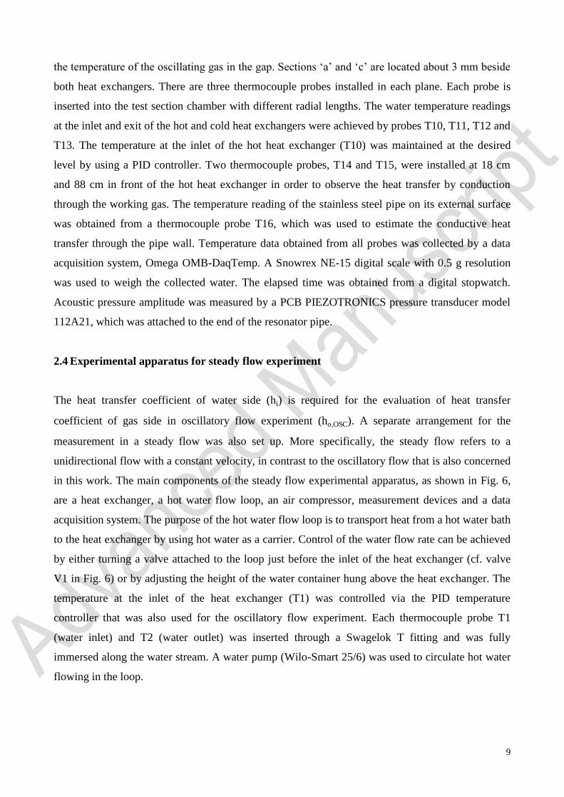
Table 2: Heat exchanger specifications.
Parameters Heat exchanger
HEX-1 HEX-2 HEX-3
Spacing between fins, D (mm) 0.7 1.4 2.1
Fin thickness, t (mm) 0.3 0.3 0.3
Fin length, L (mm) 20 20 20
Copper tube outer diameter, Do (mm) 6 6 6
Copper tube inner diameter, Di (mm) 5 5 5
Gas flow area (excluding copper pipes), Amin
(mm2) 830 950 1,015
Copper tube unfinned area, At,o
(mm2) 1,742 2,111 2,217
Copper tube water side area, At,i (mm2) 2,090 2,090 2,090
Fin surface area, Af (mm2) 69,129 40,742 28,778
Gas side heat transfer area, Ao (mm2) 70,871 42,853 30,995
Fin spacing hydraulic diameter, Dh (mm) 0.94 1.77 2.62
Heat exchanger porosity )( 0.64 0.75 0.79
Overall fin efficiency )( 0 0.699 0.707 0.714
2.3 Measurement instrumentation
Thermocouple probes (Type K) were installed where necessary (Fig. 4) to take temperature
readings for heat transfer analysis. The temperatures of the working gas facilitating the heat transfer
calculation were collected from three locations; sections ‘a’, ‘b’ and ‘c’ as illustrated in Fig. 4.
Section ‘b’ is located in the middle of the space between hot and cold heat exchangers to measure
Fig. 5: Finned-tube heat exchanger, HEX-3. The fin spacing is 2.1 mm.
9
the temperature of the oscillating gas in the gap. Sections ‘a’ and ‘c’ are located about 3 mm beside
both heat exchangers. There are three thermocouple probes installed in each plane. Each probe is
inserted into the test section chamber with different radial lengths. The water temperature readings
at the inlet and exit of the hot and cold heat exchangers were achieved by probes T10, T11, T12 and
T13. The temperature at the inlet of the hot heat exchanger (T10) was maintained at the desired
level by using a PID controller. Two thermocouple probes, T14 and T15, were installed at 18 cm
and 88 cm in front of the hot heat exchanger in order to observe the heat transfer by conduction
through the working gas. The temperature reading of the stainless steel pipe on its external surface
was obtained from a thermocouple probe T16, which was used to estimate the conductive heat
transfer through the pipe wall. Temperature data obtained from all probes was collected by a data
acquisition system, Omega OMB-DaqTemp. A Snowrex NE-15 digital scale with 0.5 g resolution
was used to weigh the collected water. The elapsed time was obtained from a digital stopwatch.
Acoustic pressure amplitude was measured by a PCB PIEZOTRONICS pressure transducer model
112A21, which was attached to the end of the resonator pipe.
2.4 Experimental apparatus for steady flow experiment
The heat transfer coefficient of water side (hi) is required for the evaluation of heat transfer
coefficient of gas side in oscillatory flow experiment (ho,OSC). A separate arrangement for the
measurement in a steady flow was also set up. More specifically, the steady flow refers to a
unidirectional flow with a constant velocity, in contrast to the oscillatory flow that is also concerned
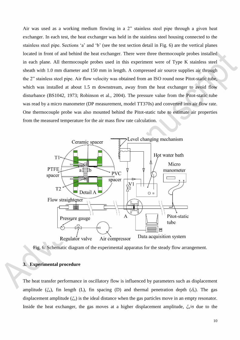
in this work. The main components of the steady flow experimental apparatus, as shown in Fig. 6,
are a heat exchanger, a hot water flow loop, an air compressor, measurement devices and a data
acquisition system. The purpose of the hot water flow loop is to transport heat from a hot water bath
to the heat exchanger by using hot water as a carrier. Control of the water flow rate can be achieved
by either turning a valve attached to the loop just before the inlet of the heat exchanger (cf. valve
V1 in Fig. 6) or by adjusting the height of the water container hung above the heat exchanger. The
temperature at the inlet of the heat exchanger (T1) was controlled via the PID temperature
controller that was also used for the oscillatory flow experiment. Each thermocouple probe T1
(water inlet) and T2 (water outlet) was inserted through a Swagelok T fitting and was fully
immersed along the water stream. A water pump (Wilo-Smart 25/6) was used to circulate hot water
flowing in the loop.
10
Air was used as a working medium flowing in a 2” stainless steel pipe through a given heat
exchanger. In each test, the heat exchanger was held in the stainless steel housing connected to the
stainless steel pipe. Sections ‘a’ and ‘b’ (see the test section detail in Fig. 6) are the vertical planes
located in front of and behind the heat exchanger. There were three thermocouple probes installed
in each plane. All thermocouple probes used in this experiment were of Type K stainless steel
sheath with 1.0 mm diameter and 150 mm in length. A compressed air source supplies air through
the 2” stainless steel pipe. Air flow velocity was obtained from an ISO round nose Pitot-static tube,
which was installed at about 1.5 m downstream, away from the heat exchanger to avoid flow
disturbance (BS1042, 1973; Robinson et al., 2004). The pressure value from the Pitot-static tube
was read by a micro manometer (DP measurement, model TT370s) and converted into air flow rate.
One thermocouple probe was also mounted behind the Pitot-static tube to estimate air properties
from the measured temperature for the air mass flow rate calculation.
3. Experimental procedure
The heat transfer performance in oscillatory flow is influenced by parameters such as displacement
amplitude (ȟa), fin length (L), fin spacing (D) and thermal penetration depth (ț). The gas
displacement amplitude (ȟa) is the ideal distance when the gas particles move in an empty resonator.
Inside the heat exchanger, the gas moves at a higher displacement amplitude, ȟa/j due to the
Fig. 6: Schematic diagram of the experimental apparatus for the steady flow arrangement.
11
porosity (j) of the heat exchanger or the reduced flow area. A small gap (2g = 5 mm) was left
between the hot and cold heat exchangers to prevent the thermal contact. Thus, from the heat
transfer point of view, the effective gas displacement inside a heat exchanger is (ȟa - g)/j. In the
normalized term, there are two parameters for the geometry of the heat exchangers, which are kD /
and ) /()( Lga . To investigate the effects of kD / and ) /()( Lga on the heat transfer
performance, measurements for the heat transfer rate were carried out, when these two
dimensionless parameters varied.
3.1 Oscillatory flow experiment
The experiment was conducted with a combination of two selected heat exchangers which were
installed in the heat exchanger housing. After installing the selected heat exchangers in the test
section and assembling the heat exchanger housing with the resonator, some air would still remain
in the system. As the working fluid in this study was pure helium gas, the remaining air in the
resonator was removed by a vacuum pump.
One of the variables to be controlled in the experiment was the normalized fin spacing which is the
ratio of fin spacing (D) to the thermal penetration depth )( k . The latter is defined by Eq.(1) and it
clearly depends on both the pressure (through changes in density) and the frequency.
pm
k c
k
2
(1)
where k, m , cp and are the thermal conductivity, density and isobaric specific heat of helium gas
and the angular frequency. The quantity k is the perpendicular distance from the plate surface,
within which heat can diffuse through the gas during a time which is of the order of an oscillation
period, fT /1 , where f is the oscillation frequency.
According to Swift (2001), the optimal value of the fin spacing is about two to four times the
thermal penetration depth )4/2( kD . Hence, the value of normalized fin spacing )/( kD in this
study ranged from 1.0 to 6.0 – which covered the suggested value. However, the highest kD / for
set ‘A’ heat exchanger was 3.5 as it was limited by the maximum design mean pressure of the
experimental apparatus.
12
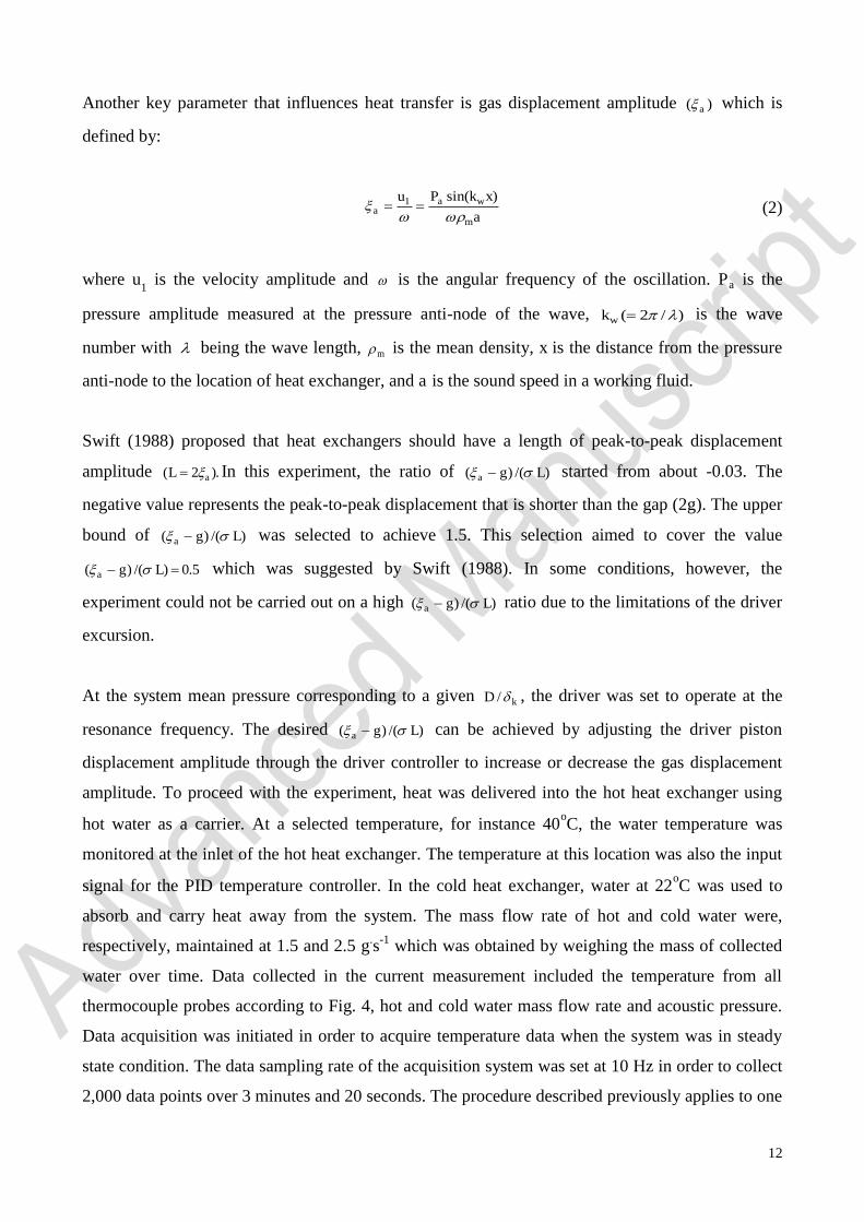
Another key parameter that influences heat transfer is gas displacement amplitude )( a which is
defined by:
a
xkPu
m
waa
)sin(1 (2)
where u1 is the velocity amplitude and is the angular frequency of the oscillation. Pa is the
pressure amplitude measured at the pressure anti-node of the wave, )/2(w k is the wave
number with being the wave length, m is the mean density, x is the distance from the pressure
anti-node to the location of heat exchanger, and a is the sound speed in a working fluid.
Swift (1988) proposed that heat exchangers should have a length of peak-to-peak displacement
amplitude ).2( aL In this experiment, the ratio of ) /()( Lga started from about -0.03. The
negative value represents the peak-to-peak displacement that is shorter than the gap (2g). The upper
bound of ) /()( Lga was selected to achieve 1.5. This selection aimed to cover the value
5.0) /()( Lga which was suggested by Swift (1988). In some conditions, however, the
experiment could not be carried out on a high ) /()( Lga ratio due to the limitations of the driver
excursion.
At the system mean pressure corresponding to a given kD / , the driver was set to operate at the
resonance frequency. The desired ) /()( Lga can be achieved by adjusting the driver piston
displacement amplitude through the driver controller to increase or decrease the gas displacement
amplitude. To proceed with the experiment, heat was delivered into the hot heat exchanger using
hot water as a carrier. At a selected temperature, for instance 40oC, the water temperature was
monitored at the inlet of the hot heat exchanger. The temperature at this location was also the input
signal for the PID temperature controller. In the cold heat exchanger, water at 22oC was used to
absorb and carry heat away from the system. The mass flow rate of hot and cold water were,
respectively, maintained at 1.5 and 2.5 g.s-1 which was obtained by weighing the mass of collected
water over time. Data collected in the current measurement included the temperature from all
thermocouple probes according to Fig. 4, hot and cold water mass flow rate and acoustic pressure.
Data acquisition was initiated in order to acquire temperature data when the system was in steady
state condition. The data sampling rate of the acquisition system was set at 10 Hz in order to collect
2,000 data points over 3 minutes and 20 seconds. The procedure described previously applies to one
13
data point in a single operating condition. At the same operating condition, the measurement was
repeated two more times. Data to be used for subsequent analysis were obtained from the average
value of the three repeated measurements.
The next test point was completed by exciting the driver to achieve a higher gas displacement
amplitude corresponding to the required ) /()( Lga . The measurement for a selected value of
kD / is completed when the data collection is carried out for the whole range of ) /()( Lga
considered. Once the measurement is completed a given kD / , the next cycle is carried out at a
next value of kD / . A desired value of kD / can be achieved by pressurizing the system with
helium gas corresponding to the desired k . After all experimental data for the inlet temperature of
40oC was obtained, the subsequent measurements were performed for the hot heat exchanger inlet
temperatures of 60 and 80oC. This experiment was designed to be performed on three
configurations of heat exchanger. To complete the test on the other two configurations, the first set
of heat exchanger was removed and replaced by the new set. After installing the new configuration
and assembling the test section, the leakage test and the removal of air from the resonator were
carried out. The experimental procedure for the rest of the heat exchangers was similar to that
explained above.
3.2 Steady flow experiment
In order to determine heat transfer performance in an oscillatory flow condition, the value of the
water side heat transfer coefficient (hi) needs to be known in advance. The experiment in steady
flow conditions was introduced as follows. To carry out one batch of steady flow tests, a selected
heat exchanger was installed in the stainless steel housing. Heat was supplied to the heat exchanger
by hot water flowing inside the tube while the air flowing through fins absorbed and carried heat
away from the test section. According to Fig. 6, air temperatures at upstream and downstream of the
heat exchanger were obtained from thermocouples at sections ‘a’ and ‘b’, while thermocouples T1
and T2 were also used to measure the inlet and outlet temperature of the water, respectively. Water
mass flow rate through the heat exchanger was obtained by weighing the mass of collected water
and dividing it by the time period elapsed.
The first test on the heat exchanger with a fin spacing of 0.7 mm was performed at the lowest water
inlet temperature of 40oC. The water pump was turned on to circulate hot water through the heat
exchanger loop. While waiting for the temperature to reach the set value, the water mass flow rate
14
was adjusted either by controlling a valve (cf. valve V1 in Fig. 6) or by changing the level of the
water storage container that hung above the heat exchanger.
As far as the air side is concerned, the air compressor was turned on and left running until it reached
its maximum pressure capacity. The air flow rate was set to start the test at the minimum flow rate.
Air flow rate was controlled by using a regulator valve on the air compressor. After running the
system for a period of time, the operator should monitor temperature variation for all measuring
points. If the temperature profile exhibits stable trend, the flow rates of water and air are checked to
make sure they are flowing at the required values. When the temperature and flow rate are achieved,
the temperature data collection begins by initiating the data acquisition system. This procedure
constitutes the measurement of one data point. The next test was carried out by slightly increasing
the water flow rate. The range of the water mass flow rate must cover the flow rate designed for the
oscillatory flow experiment. The next sets of measurement were performed at a higher air flow rate
and the cycle was repeated. When the test at the maximum air flow rate and a water inlet
temperature at 40oC was completed, the experiment was then carried out for the higher temperatures
of 60 and 80oC. The whole procedure was repeated for heat exchangers with fin spacing of 1.4 and
2.1 mm to complete the data collection in the steady flow experiment.
4. Data reduction
Data reduction for steady flow experiment is presented first in order to obtain the water side heat
transfer coefficient (hi). It will facilitate the heat transfer performance evaluation in oscillatory flow
which is illustrated in Section 4.2.
4.1 Steady flow
The aim of the current study is to develop measurement techniques for heat transfer when the
working gas experiences an oscillating flow. The heat transfer coefficient for water side (hi) is
required prior to calculating the heat transfer performance in oscillatory flow conditions. The data
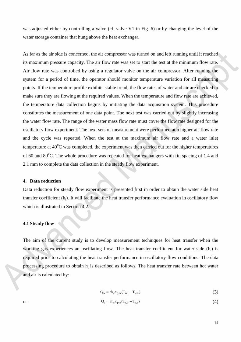
processing procedure to obtain hi is described as follows. The heat transfer rate between hot water
and air is calculated by:
)( ,,, owiwwpww TTcmQ (3)
or )( ,,, iaoaapaa TTcmQ (4)
15
The subscripts w, a, i and o in above equations denote water, air, and the location at the inlet and
outlet of the fluid stream, respectively. cp,w and cp,a are specific heat capacity at constant pressure
of water and air. The mass flow rate of water is achieved by weighing the mass of collected water
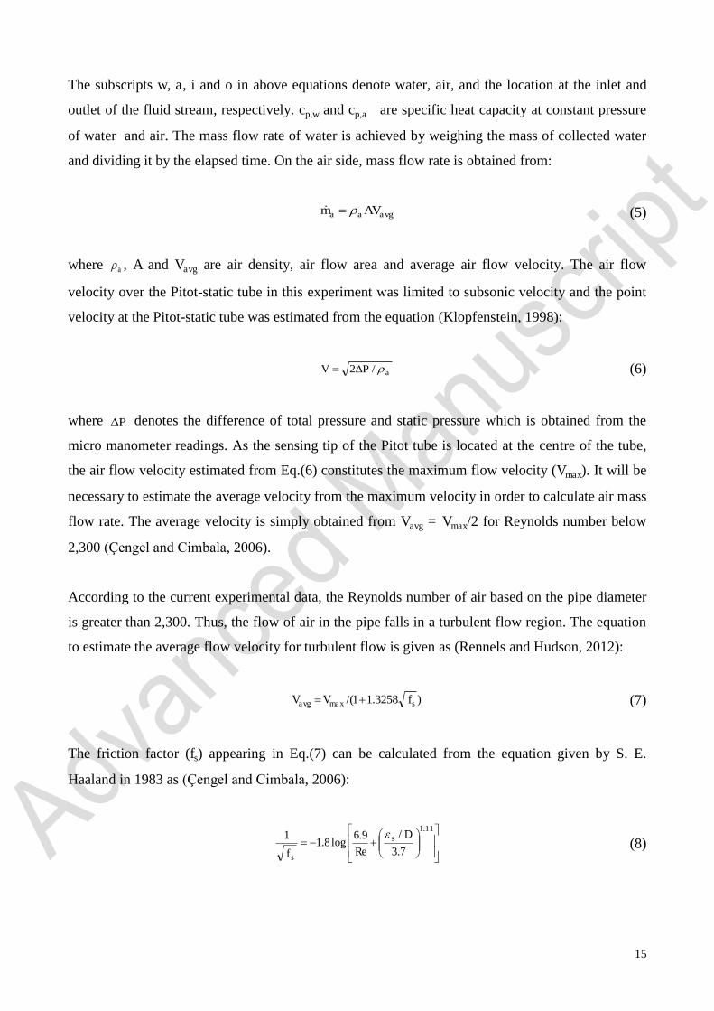
and dividing it by the elapsed time. On the air side, mass flow rate is obtained from:
avgaa AVm (5)
where a , A and Vavg are air density, air flow area and average air flow velocity. The air flow
velocity over the Pitot-static tube in this experiment was limited to subsonic velocity and the point
velocity at the Pitot-static tube was estimated from the equation (Klopfenstein, 1998):
aPV /2 (6)
where P denotes the difference of total pressure and static pressure which is obtained from the
micro manometer readings. As the sensing tip of the Pitot tube is located at the centre of the tube,
the air flow velocity estimated from Eq.(6) constitutes the maximum flow velocity (Vmax). It will be
necessary to estimate the average velocity from the maximum velocity in order to calculate air mass
flow rate. The average velocity is simply obtained from Vavg = Vmax/2 for Reynolds number below
2,300 (̧engel and Cimbala, 2006).
According to the current experimental data, the Reynolds number of air based on the pipe diameter
is greater than 2,300. Thus, the flow of air in the pipe falls in a turbulent flow region. The equation
to estimate the average flow velocity for turbulent flow is given as (Rennels and Hudson, 2012):
)3258.11/( smaxavg fVV (7)
The friction factor (fs) appearing in Eq.(7) can be calculated from the equation given by S. E.
Haaland in 1983 as (̧engel and Cimbala, 2006):
11.1
7.3
/9.6 log8.1
1 D
Ref
s
s
(8)
16
where the absolute roughness )( s of the PVC pipe is 0.0015 mm (Rennels and Hudson, 2012). To
obtain the average air flow velocity, an iterative process in Eq.(7) and (8) is required as the
unknown air flow velocity is integrated in the Reynolds number in Eq.(8).
The heat transfer in the heat exchanger used in the current experiment involves the thermal
resistance consisting of three parts: the resistance for heat transfer from water to the wall of copper
tube, thermal resistance of copper tube and the resistance for heat transfer from copper tube to air. It
is useful to apply an overall heat transfer coefficient concept as (Paek et al., 2005 and Mao et al.,
2011):
it
di
tubeo
bSTDoo
STD
ARecR
ARea
RUA
LMTD
Q
,, )(
1
)(
111
(9)
In Eq.(9), air side Reynolds number (Reo,STD) is based on the fin spacing hydraulic diameter (Dh),
while water side Reynolds number (Rei) is based on copper tube inside diameter (Di). The
logarithmic mean temperature difference (LMTDSTD
) is given by:
iaow
oaiw
iaowoaiwSTD
TT
TT
TTTTFLMTD
,,
,,
,,,,
ln
(10)
The correction factor (F) is introduced so that the LMTDSTD is suitable for the cross flow
arrangement. It is approximately 0.98 (̧engel, 1997). Thermal resistance of copper tube is obtained
by:
kLrrR Ttube 2/ln 12 (11)
where r2 and r1 are the outside and inside tube radii. LT denotes the effective tube length where the
heat transfer to/from the air occurs and k is the thermal conductivity of the copper tube.
The overall fin efficiency )( o is obtained from (Incropera, 2006):
)1(1 fo
fo A
A (12)
17
where Af and A
o are fin surface area and air side heat transfer area (fin surface area plus the area of
copper tube contacts with air). The efficiency of a single fin )( f is calculated from:
c
cf mL
mLtanh )( (13)
where cmL is expressed by:
cfc
c LAk
hmL
0 (14)
In Eq.(14), ho is the convective heat transfer coefficient and k is the thermal conductivity of fin
material. Geometrical parameters Afc, and Lc denote fin cross sectional area, fin cross sectional
perimeter and corrected fin length, respectively. When the fin is considered having convection heat
transfer at its tip, the corrected fin length (Lc) can be found from:
Lc = L + (t/2) (15)
where L and t are the fin length and fin thickness, respectively.
From Eq.(9), Q and LMTDSTD are calculated from Eq.(3) and Eq.(10) using measured data. Then,
parameters a, b, c and d are obtained by non-linear surface fitting using the simplex method in
software package ‘Origin’. The heat transfer coefficient of the air side (ho,STD) and the water side
(hi) can be defined as:
bSTDoSTDo Reah ,, (16)
dii Rech (17)
4.2 Oscillatory flow
In oscillatory flow experiment, heat carried by the hot water stream inside the tube of the hot heat
exchanger is transferred to the oscillating gas. The oscillating gas works as a carrier to transport
heat between the hot and cold heat exchangers. Then, the heat is absorbed at the cold heat
18
exchanger and ejected to the external heat sink. Heat transfer rate in oscillatory flow is calculated
from the water side of hot heat exchanger following Eq.(3). The measurement on cold heat
exchanger is possible but less accurate. This is due to the cold water flow rate being maintained at a
higher value than that of the hot water. As a result, the temperature difference between the inlet and
exit of the cold heat exchanger was small, leading to high uncertainty in the heat transfer rate.
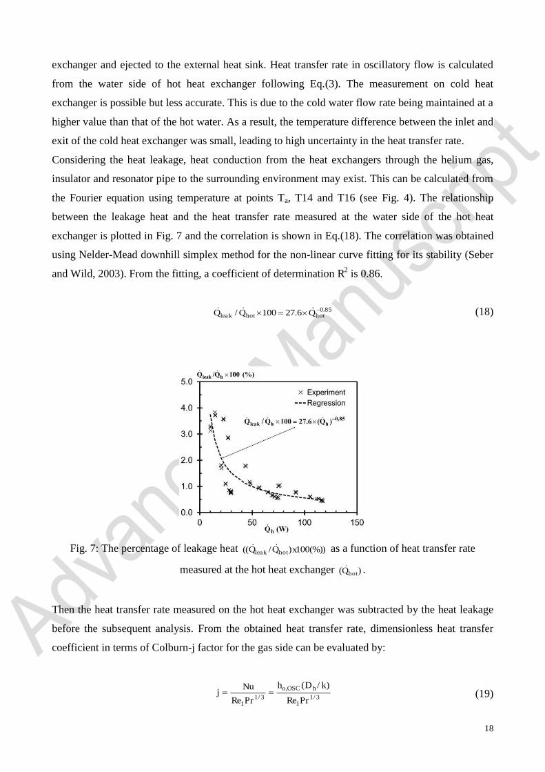
Considering the heat leakage, heat conduction from the heat exchangers through the helium gas,
insulator and resonator pipe to the surrounding environment may exist. This can be calculated from
the Fourier equation using temperature at points Ta, T14 and T16 (see Fig. 4). The relationship
between the leakage heat and the heat transfer rate measured at the water side of the hot heat
exchanger is plotted in Fig. 7 and the correlation is shown in Eq.(18). The correlation was obtained
using Nelder-Mead downhill simplex method for the non-linear curve fitting for its stability (Seber
and Wild, 2003). From the fitting, a coefficient of determination R2 is 0.86.
85.06.27100/ hothotleak QQQ (18)
Then the heat transfer rate measured on the hot heat exchanger was subtracted by the heat leakage
before the subsequent analysis. From the obtained heat transfer rate, dimensionless heat transfer
coefficient in terms of Colburn-j factor for the gas side can be evaluated by:
3/11
,
3/11
)/(
PrRe
kDh
PrRe
Nuj hOSCo (19)
Fig. 7: The percentage of leakage heat (%))100)/(( xQQ hotleak as a function of heat transfer rate
measured at the hot heat exchanger )( hotQ .
19
Acoustic Reynolds number (Re1) is expressed by:
1
1uD
Re h (20)
where u1 denotes acoustic velocity amplitude.
To find the gas side heat transfer coefficient in oscillatory flow (ho,OSC), the overall heat transfer
coefficient is employed on the hot heat exchanger as follows:
ii
tubeoOSCoo
OSC
AhR
Ah
UALMTD
Q11
1
,
(21)
The log-mean temperature difference LMTDOSC
is defined as:
owb
iwb
iwowOSC
TT
TT
TTLMTD
,
,
,,
ln
(22)
Tb is the temperature of the gas at section ‘b’ according to Fig. 4, while Tw,i and Tw,o denote the
temperature of water measured at the inlet (T10) and exit (T11) of the hot heat exchanger,
respectively. The heat transfer coefficient for the water side (hi) can be obtained from Eq.(17) which
was developed from the steady flow experiment.
5. Measurement uncertainty
Measurement uncertainty is performed to estimate errors in the experimental results. The
uncertainty consists of several components which can be categorized into two groups: precision or
random uncertainty, and systematic or fixed uncertainty (Rood and Telionis, 1991 and Kim et al.,
1993). From Eq.(3), the uncertainty )( QU of heat transfer rate )(Q is given by the combination of a
precision uncertainty )( Qs , and a systematic uncertainty )( Qb .
20
2/122 )( QQQ bsU (23)
The estimations of the precision and systematic uncertainty are made according to the error
propagation equation (Kline and McClintock, 1953) as follows.
222222222 )/()/()/()/(iTioTopcpmQ sTQsTQscQsmQs
(24)
and 222222222 )/()/()/()/(iTioToppmQ bTQbTQcbcQbmQb
(25)
where ms , sTo and sTi are the elemental precision uncertainty of m , To and Ti, respectively. The
partial derivations appeared in Eq.(24) and (25) are the sensitivity coefficient which represent the
change of the result )(Q when the value of a particular elemental measurement parameter is varied.
The uncertainties of elemental parameters are described as follows.
5.1 Uncertainty of water mass flow rate measurement
The water mass flow rate )( m present in Eq. (3) is obtained from the mass of collected water (m)
over the elapsed time (t) by tmm / . Applying the error propagation approach, the precision
uncertainty )( ms and systematic uncertainty )( mb of the water mass flow rate measurement can be
found by:
2
22
22
tmm st
ms
m
ms
(26)
and 22
22
2tmm b
t
mb
m
mb
(27)
where sm and st are the precision uncertainty of mass and time measurement, and bm and bt are the
systematic uncertainty of mass and time measurement, respectively.
In mass flow rate measurement, the systematic uncertainty of mass (bm) and time (bt) measurements
are omitted because the digital scale and the stop watch were calibrated. Precision uncertainty for
mass (sm) and time (st) measurement is calculated from a series of repeated observations using
statistical methods. The precision uncertainty of mass measurement (sm), due to repeatability, is
21
evaluated through the sample standard deviation (Sm) of the repeated mass measurement results
from Eq. (28) (Miller, 2002).
NSs mm / (28)
where N is a number of samples. For the measurement of elapsed time, the precision uncertainty (st)
arises from the reaction time of the operator when pressing the start/stop button of the stop watch.
The procedure to evaluate for st follows the instruction as reported by Gust et al. (2004).
5.2 Uncertainty of isobaric specific heat of water
In this experiment, the variable isobaric specific heat capacity (cp) was estimated by an equation
(Richardson, 2010). The specific heat value of water was calculated using the average temperature
of the inlet and exit of a heat exchanger as an input value. Thus, there may be an uncertainty in the
specific heat capacity estimated from the average temperature. As the value of cp is obtained from
the equation, the precision uncertainty (scp) is neglected. Another source of error stems from the
accuracy of the curve-fitting equation. This kind of error is considered to be a systematic
uncertainty in the specific heat capacity value. In some published sources (Angell et al., 1982;
Archer and Carter, 2000), the uncertainty of specific heat capacity is presented in the form of a
percentage departure of experimental data from the values calculated from the curve-fitting
equation. According to Wagner (2002), the systematic uncertainty of water specific heat capacity
(bcp), estimated at 95% confidence, corresponding to the current experimental conditions is ±0.4%
of the calculated value.
5.3 Uncertainty of temperature measurement
In order to calculate the heat transfer rate according to Eq. (3), the measurement of water
temperature at the inlet and exit points needs to be acquired. Similar to other variables, the errors
inherent in temperature measurement originate from the precision and systematic errors. The
precision uncertainty is estimated from the standard deviation of samples for temperature
measurement. Systematic uncertainty is embedded in temperature measurements. The value of
systematic uncertainty does not vary and it cannot be directly determined by measurements or any
statistical technique. The systematic uncertainty is influenced by the calibration standard of the
thermocouple probes which is achieved from the thermocouple specification supplied by the
22
manufacturer. Following the procedure suggested by Kim et al. (1993) and Coleman and Steele
(2009), the systematic uncertainty for temperature measurement (bTi and bTo) obtained from type K
thermocouple probes used in this experiment is evaluated at ±0.55oC based on the 95% confidence
level.
5.4 Uncertainty of heat transfer rate
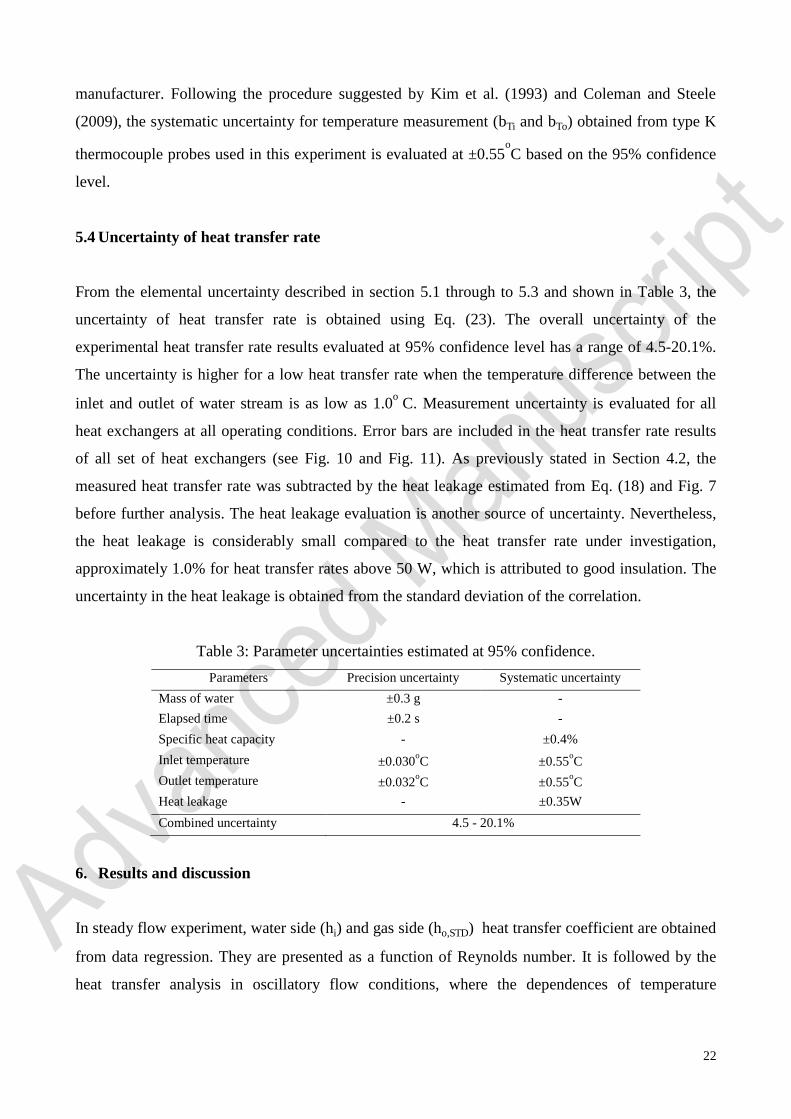
From the elemental uncertainty described in section 5.1 through to 5.3 and shown in Table 3, the
uncertainty of heat transfer rate is obtained using Eq. (23). The overall uncertainty of the
experimental heat transfer rate results evaluated at 95% confidence level has a range of 4.5-20.1%.
The uncertainty is higher for a low heat transfer rate when the temperature difference between the
inlet and outlet of water stream is as low as 1.0o C. Measurement uncertainty is evaluated for all
heat exchangers at all operating conditions. Error bars are included in the heat transfer rate results
of all set of heat exchangers (see Fig. 10 and Fig. 11). As previously stated in Section 4.2, the
measured heat transfer rate was subtracted by the heat leakage estimated from Eq. (18) and Fig. 7
before further analysis. The heat leakage evaluation is another source of uncertainty. Nevertheless,
the heat leakage is considerably small compared to the heat transfer rate under investigation,
approximately 1.0% for heat transfer rates above 50 W, which is attributed to good insulation. The
uncertainty in the heat leakage is obtained from the standard deviation of the correlation.
Table 3: Parameter uncertainties estimated at 95% confidence.
Parameters Precision uncertainty Systematic uncertainty
Mass of water ±0.3 g -
Elapsed time ±0.2 s -
Specific heat capacity - ±0.4%
Inlet temperature ±0.030oC ±0.55oC
Outlet temperature ±0.032oC ±0.55oC
Heat leakage - ±0.35W
Combined uncertainty 4.5 - 20.1%
6. Results and discussion
In steady flow experiment, water side (hi) and gas side (ho,STD) heat transfer coefficient are obtained
from data regression. They are presented as a function of Reynolds number. It is followed by the
heat transfer analysis in oscillatory flow conditions, where the dependences of temperature
23
measured at different locations, heat transfer rate and Coburn-j factor on ) /()( Lga and kD / are
presented.
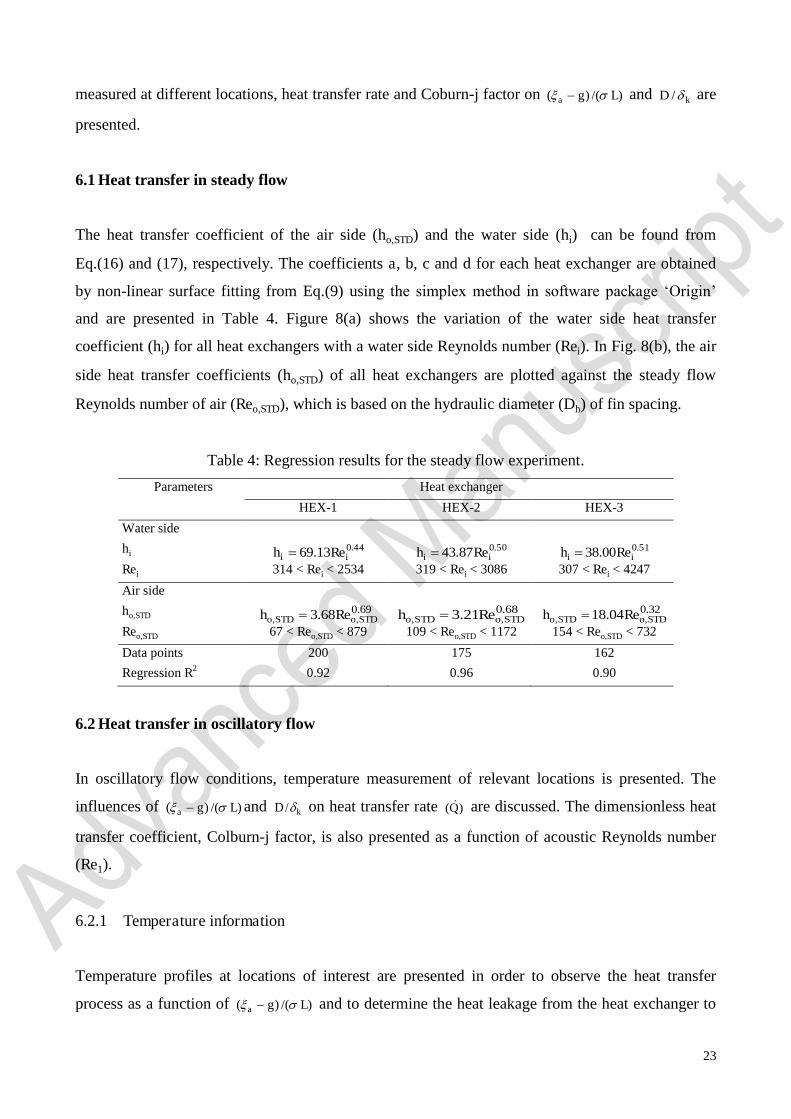
6.1 Heat transfer in steady flow
The heat transfer coefficient of the air side (ho,STD) and the water side (hi) can be found from
Eq.(16) and (17), respectively. The coefficients a, b, c and d for each heat exchanger are obtained
by non-linear surface fitting from Eq.(9) using the simplex method in software package ‘Origin’
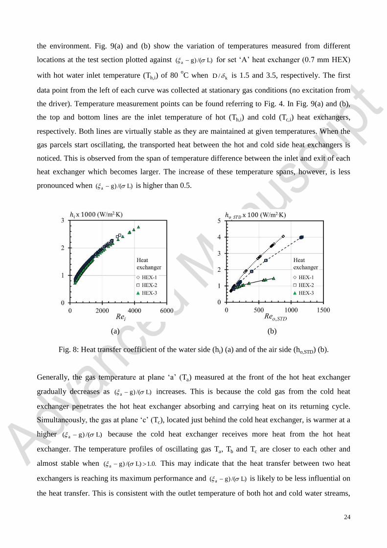
and are presented in Table 4. Figure 8(a) shows the variation of the water side heat transfer
coefficient (hi) for all heat exchangers with a water side Reynolds number (Rei). In Fig. 8(b), the air
side heat transfer coefficients (ho,STD) of all heat exchangers are plotted against the steady flow
Reynolds number of air (Reo,STD), which is based on the hydraulic diameter (Dh) of fin spacing.
Table 4: Regression results for the steady flow experiment.
Parameters Heat exchanger
HEX-1 HEX-2 HEX-3
Water side
hi 44.013.69 ii Reh 50.087.43 ii Reh 51.000.38 ii Reh Rei 314 < Rei < 2534 319 < Rei < 3086 307 < Rei < 4247
Air side
ho,STD 69.0,, 68.3 STDoSTDo Reh 68.0
,, 21.3 STDoSTDo Reh 32.0,, 04.18 STDoSTDo Reh
Reo,STD 67 < Reo,STD < 879 109 < Reo,STD < 1172 154 < Reo,STD < 732
Data points 200 175 162
Regression R2 0.92 0.96 0.90
6.2 Heat transfer in oscillatory flow
In oscillatory flow conditions, temperature measurement of relevant locations is presented. The
influences of ) /()( Lga and kD / on heat transfer rate )(Q are discussed. The dimensionless heat
transfer coefficient, Colburn-j factor, is also presented as a function of acoustic Reynolds number
(Re1).
6.2.1 Temperature information
Temperature profiles at locations of interest are presented in order to observe the heat transfer
process as a function of ) /()( Lga and to determine the heat leakage from the heat exchanger to
24
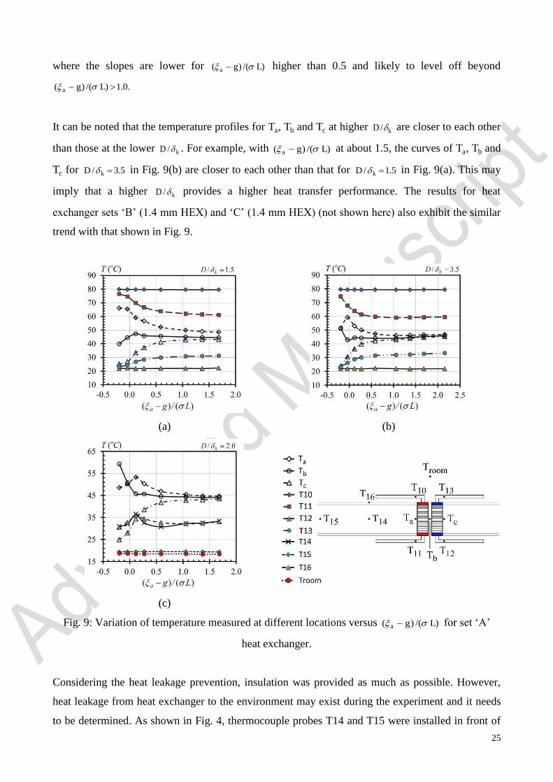
the environment. Fig. 9(a) and (b) show the variation of temperatures measured from different
locations at the test section plotted against ) /()( Lga for set ‘A’ heat exchanger (0.7 mm HEX)
with hot water inlet temperature (Th,i) of 80 oC when kD / is 1.5 and 3.5, respectively. The first
data point from the left of each curve was collected at stationary gas conditions (no excitation from
the driver). Temperature measurement points can be found referring to Fig. 4. In Fig. 9(a) and (b),
the top and bottom lines are the inlet temperature of hot (Th,i) and cold (Tc,i) heat exchangers,
respectively. Both lines are virtually stable as they are maintained at given temperatures. When the
gas parcels start oscillating, the transported heat between the hot and cold side heat exchangers is
noticed. This is observed from the span of temperature difference between the inlet and exit of each
heat exchanger which becomes larger. The increase of these temperature spans, however, is less
pronounced when ) /()( Lga is higher than 0.5.
(a) (b)
Fig. 8: Heat transfer coefficient of the water side (hi) (a) and of the air side (ho,STD) (b).
Generally, the gas temperature at plane ‘a’ (Ta) measured at the front of the hot heat exchanger
gradually decreases as ) /()( Lga increases. This is because the cold gas from the cold heat
exchanger penetrates the hot heat exchanger absorbing and carrying heat on its returning cycle.
Simultaneously, the gas at plane ‘c’ (Tc), located just behind the cold heat exchanger, is warmer at a
higher ) /()( Lga because the cold heat exchanger receives more heat from the hot heat
exchanger. The temperature profiles of oscillating gas Ta, Tb and Tc are closer to each other and
almost stable when .0.1) /()( Lga This may indicate that the heat transfer between two heat
exchangers is reaching its maximum performance and ) /()( Lga is likely to be less influential on
the heat transfer. This is consistent with the outlet temperature of both hot and cold water streams,
25
where the slopes are lower for ) /()( Lga higher than 0.5 and likely to level off beyond
.0.1) /()( Lga
It can be noted that the temperature profiles for Ta, Tb and Tc at higher kD / are closer to each other
than those at the lower kD / . For example, with ) /()( Lga at about 1.5, the curves of Ta, Tb and
Tc for 5.3/ kD in Fig. 9(b) are closer to each other than that for 5.1/ kD in Fig. 9(a). This may
imply that a higher kD / provides a higher heat transfer performance. The results for heat
exchanger sets ‘B’ (1.4 mm HEX) and ‘C’ (1.4 mm HEX) (not shown here) also exhibit the similar
trend with that shown in Fig. 9.
(a) (b)
(c)
Fig. 9: Variation of temperature measured at different locations versus ) /()( Lga for set ‘A’
heat exchanger.
Considering the heat leakage prevention, insulation was provided as much as possible. However,
heat leakage from heat exchanger to the environment may exist during the experiment and it needs
to be determined. As shown in Fig. 4, thermocouple probes T14 and T15 were installed in front of
26
the hot heat exchanger in order to estimate the conductive heat transfer through the gas. The
temperature of the external surface of the stainless steel resonator, detected by T16, and room
temperature were also collected simultaneously.
Fig. 9(c) shows temperature variation on set ‘A’ heat exchanger for selected locations. It can be
seen that the curves for temperature of gas measured at the point in front of the hot heat exchanger
(T14) and of the resonator external surface (T16) have similar trend with the gas temperature
measured at section ‘a’ (Ta) but smaller in magnitude. This indicates some heat leakage via the
conduction from the hot heat exchanger through the gas and the stainless steel pipe. The
temperature of gas further away from the hot heat exchanger was obtained from the thermocouple
probe T15 and found to be very close to room temperature (Troom). Thus, the conductive heat
transfer in gas from T14 to T15 was considered small. The relative heat leakage )( leakQ as a
function of measured heat transfer rate )( hotQ was shown in Fig. 7. The heat transfer rate measured
on the hot heat exchanger )( hotQ was then corrected by the heat leakage )( leakQ before subsequent
analysis.
6.2.2 The influence of ) /()( Lga on heat transfer rate )(Q
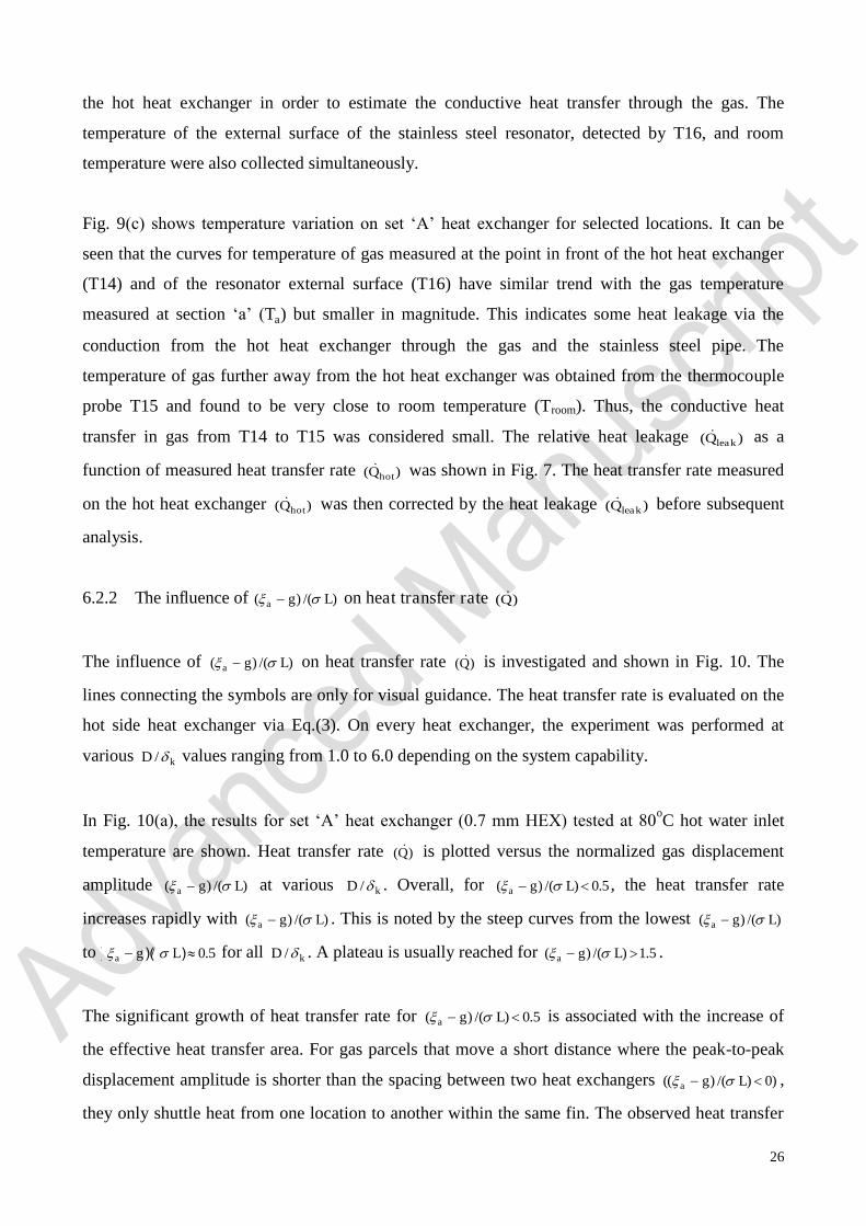
The influence of ) /()( Lga on heat transfer rate )(Q is investigated and shown in Fig. 10. The
lines connecting the symbols are only for visual guidance. The heat transfer rate is evaluated on the
hot side heat exchanger via Eq.(3). On every heat exchanger, the experiment was performed at
various kD / values ranging from 1.0 to 6.0 depending on the system capability.
In Fig. 10(a), the results for set ‘A’ heat exchanger (0.7 mm HEX) tested at 80oC hot water inlet
temperature are shown. Heat transfer rate )(Q is plotted versus the normalized gas displacement
amplitude ) /()( Lga at various kD / . Overall, for 5.0) /()( Lga , the heat transfer rate
increases rapidly with ) /()( Lga . This is noted by the steep curves from the lowest ) /()( Lga
to 5.0 / )()( Lga for all kD / . A plateau is usually reached for 5.1) /()( Lga .
The significant growth of heat transfer rate for 5.0) /()( Lga is associated with the increase of
the effective heat transfer area. For gas parcels that move a short distance where the peak-to-peak
displacement amplitude is shorter than the spacing between two heat exchangers )0) /()(( Lga ,
they only shuttle heat from one location to another within the same fin. The observed heat transfer
27
may be attributed to heat conduction through the gas. When the gas displacement amplitude
increases, the proportion of gas parcels that have thermal contact with both heat exchangers within
their oscillating cycle is larger, thus enhancing the heat transfer rate. The heat transfer increases
steadily until 5.0 / )()( Lga where all gas parcels that have thermal contact on one heat
exchanger are able to reach the surface of the adjacent heat exchanger thus transferring heat
between them. When ,5.0) /()( Lga a fraction of gas particles jump from one heat exchanger
and pass to the farthest edge of the next heat exchanger. Hence, such parcels do not contribute to the
heat transfer between heat exchangers, and thus do not contribute to the heat transfer rate
enhancement.
(a) (b)
(c)
Fig. 10: Dependence of Q on ) /()( Lga at various kD / for Th,i = 80oC.
28
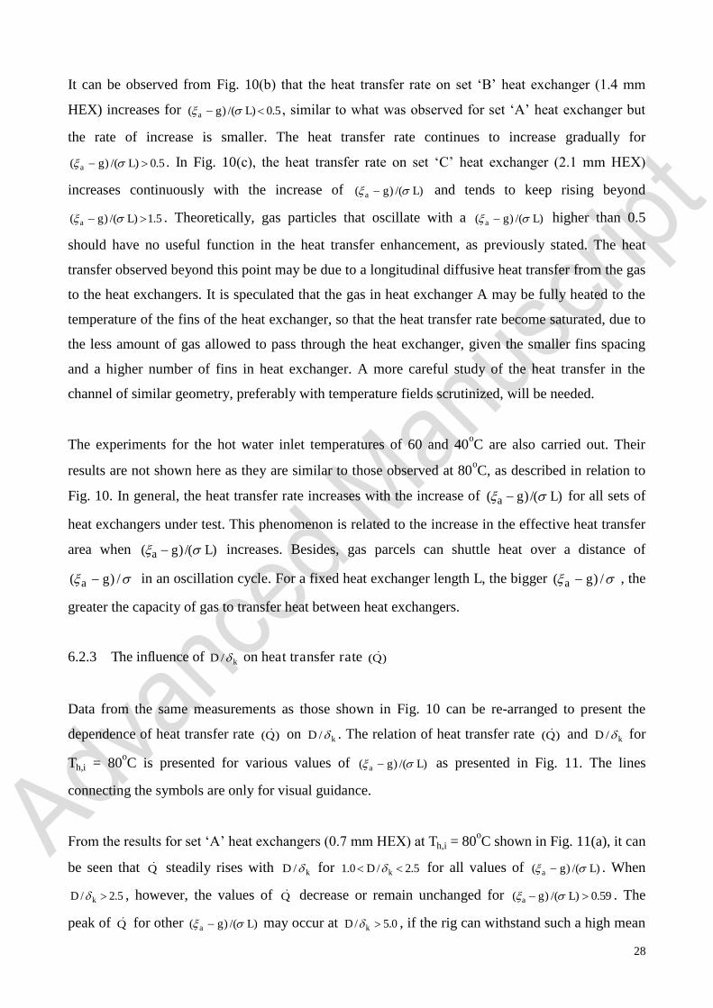
It can be observed from Fig. 10(b) that the heat transfer rate on set ‘B’ heat exchanger (1.4 mm
HEX) increases for 5.0) /()( Lga , similar to what was observed for set ‘A’ heat exchanger but
the rate of increase is smaller. The heat transfer rate continues to increase gradually for
5.0) /()( Lga . In Fig. 10(c), the heat transfer rate on set ‘C’ heat exchanger (2.1 mm HEX)
increases continuously with the increase of ) /()( Lga and tends to keep rising beyond
5.1) /()( Lga . Theoretically, gas particles that oscillate with a ) /()( Lga higher than 0.5
should have no useful function in the heat transfer enhancement, as previously stated. The heat
transfer observed beyond this point may be due to a longitudinal diffusive heat transfer from the gas
to the heat exchangers. It is speculated that the gas in heat exchanger A may be fully heated to the
temperature of the fins of the heat exchanger, so that the heat transfer rate become saturated, due to
the less amount of gas allowed to pass through the heat exchanger, given the smaller fins spacing
and a higher number of fins in heat exchanger. A more careful study of the heat transfer in the
channel of similar geometry, preferably with temperature fields scrutinized, will be needed.
The experiments for the hot water inlet temperatures of 60 and 40oC are also carried out. Their
results are not shown here as they are similar to those observed at 80oC, as described in relation to
Fig. 10. In general, the heat transfer rate increases with the increase of ) /()( Lga for all sets of
heat exchangers under test. This phenomenon is related to the increase in the effective heat transfer
area when ) /()( Lga increases. Besides, gas parcels can shuttle heat over a distance of
/)( ga in an oscillation cycle. For a fixed heat exchanger length L, the bigger /)( ga , the
greater the capacity of gas to transfer heat between heat exchangers.
6.2.3 The influence of kD / on heat transfer rate )(Q
Data from the same measurements as those shown in Fig. 10 can be re-arranged to present the
dependence of heat transfer rate )(Q on kD / . The relation of heat transfer rate )(Q and kD / for
Th,i = 80oC is presented for various values of ) /()( Lga as presented in Fig. 11. The lines
connecting the symbols are only for visual guidance.
From the results for set ‘A’ heat exchangers (0.7 mm HEX) at Th,i = 80oC shown in Fig. 11(a), it can
be seen that Q steadily rises with kD / for 5.2/0.1 kD for all values of ) /()( Lga . When
5.2/ kD , however, the values of Q decrease or remain unchanged for 59.0) /()( Lga . The
peak of Q for other ) /()( Lga may occur at 0.5/ kD , if the rig can withstand such a high mean
29
pressure, as were the case for the heat exchanger sets ‘B’ and ‘C’. The influence of kD / on Q for
set ‘B’ heat exchanger (1.4 mm HEX) is shown in Fig. 11(b). The increase of Q with kD / is
observed for the value of kD / up to 5.0. In general, it appears that 0.5/ kD seems to be the peak
of Q for most ) /()( Lga values. Fig. 11(c) shows the results for set ‘C’ heat exchangers (2.1 mm
HEX). The overall trend is similar to that seen in set ‘B’ heat exchanger (1.4 mm HEX). However,
the peak of Q for 09.0) /()( Lga tends to occur at 5.5/ kD , whereas the values of Q for
03.0) /()( Lga continue to increase with D . Generally speaking, the optimum Q for most
conditions could be between 5.50.5 D . Compared to the recommended region of
42 D (Swift, 2001), the optimal D obtained from the current study is slightly higher.
This could be due to the physical construction of the heat exchangers used, in which tubes are
connecting fins for heat supply and contribute a substantial amount to the overall heat transfer area,
whereas in the literature, the optimal range of D is based on a numerical study of heat transfer
between two parallel plates with a negligible thickness. The underlying mechanism of the difference
is not clear.
6.2.4 Dimensionless heat transfer coefficient: Colburn-j factor
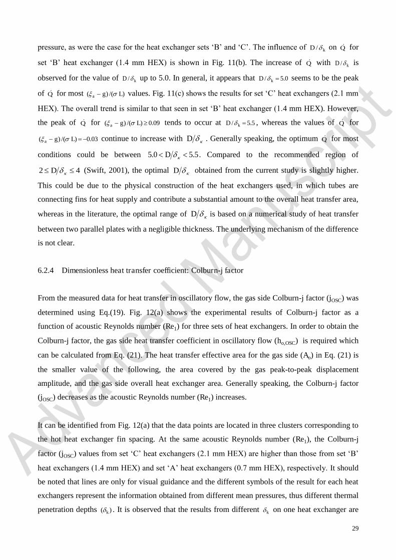
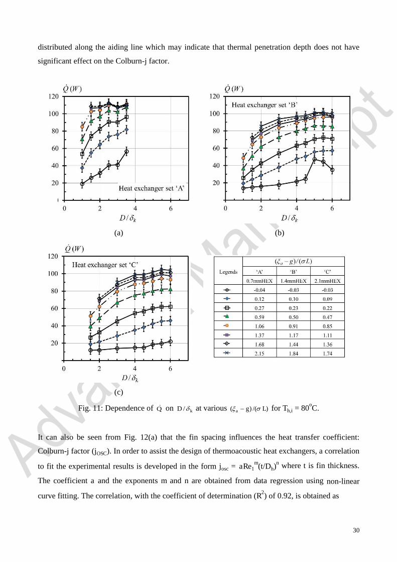
From the measured data for heat transfer in oscillatory flow, the gas side Colburn-j factor (jOSC) was
determined using Eq.(19). Fig. 12(a) shows the experimental results of Colburn-j factor as a
function of acoustic Reynolds number (Re1) for three sets of heat exchangers. In order to obtain the
Colburn-j factor, the gas side heat transfer coefficient in oscillatory flow (ho,OSC) is required which
can be calculated from Eq. (21). The heat transfer effective area for the gas side (Ao) in Eq. (21) is
the smaller value of the following, the area covered by the gas peak-to-peak displacement
amplitude, and the gas side overall heat exchanger area. Generally speaking, the Colburn-j factor
(jOSC) decreases as the acoustic Reynolds number (Re1) increases.
It can be identified from Fig. 12(a) that the data points are located in three clusters corresponding to
the hot heat exchanger fin spacing. At the same acoustic Reynolds number (Re1), the Colburn-j
factor (jOSC) values from set ‘C’ heat exchangers (2.1 mm HEX) are higher than those from set ‘B’
heat exchangers (1.4 mm HEX) and set ‘A’ heat exchangers (0.7 mm HEX), respectively. It should
be noted that lines are only for visual guidance and the different symbols of the result for each heat
exchangers represent the information obtained from different mean pressures, thus different thermal
penetration depths )( k . It is observed that the results from different k on one heat exchanger are
30
distributed along the aiding line which may indicate that thermal penetration depth does not have
significant effect on the Colburn-j factor.
(a) (b)
(c)
Fig. 11: Dependence of Q on kD / at various ) /()( Lga for Th,i = 80oC.
It can also be seen from Fig. 12(a) that the fin spacing influences the heat transfer coefficient:
Colburn-j factor (jOSC). In order to assist the design of thermoacoustic heat exchangers, a correlation
to fit the experimental results is developed in the form josc = aRe1m(t/Dh)
n where t is fin thickness.
The coefficient a and the exponents m and n are obtained from data regression using non-linear
curve fitting. The correlation, with the coefficient of determination (R2) of 0.92, is obtained as
31
josc = 0.0313Re1-0.6394(t/Dh)
-1.2541. (29)
(a) (b)
(c)
Fig. 12: Measured gas side Colburn-j factor versus acoustic Reynolds number (Re1) of three sets of
heat exchanger plotted log-log scale (a), j/(t/Dh)-1.2541 against Re1 in log-log scale (b) and Colburn-j
factor from experiment (jOSC,exp) in comparison with the estimation (jOSC,est) (c).
From the correlation and the results in Fig. 12(a), j/(t/Dh)-1.2541 is plotted versus Re1 in log-log scale
in Fig. 12(b). The family of data points corresponding to different heat exchangers can be collapsed
32
to a group of points that fall close to a single line as shown. Thus, it is expected that the proposed
correlation could help the design of finned-tube heat exchanger for oscillatory flow conditions. The
comparison of the experimental Colburn-j factor (jOSC,exp) and the estimated values (jOSC,est) is also
illustrated in Fig. 12(c) with the average deviation about 18%.
7. Conclusion
Heat exchangers are some of the most important components in thermoacoustic devices. The overall
efficiency of such devices is greatly reliant on the heat transfer performance. However, the
relationship between heat transfer and heat exchanger geometry and operating conditions is not well
understood. The current study has developed experimental apparatus and techniques to investigate
the heat transfer in oscillatory flows.
Steady flow experiment was carried out to get water side heat transfer coefficient (hi) for facilitating
the heat transfer analysis in oscillatory flow. In oscillatory flow experiment, heat transfer rates were
calculated from the water side of the hot heat exchangers at various operating conditions. The
influence of ) /()( Lga on Q was explored. For the heat exchanger set ‘A’, the values of Q
increased rapidly for 5.0) /()( Lga . The growth rate, however, was lower for the higher
) /()( Lga and almost levelled off when .5.1) /()( Lga A different trend was observed on the
heat exchanger sets ‘B’ and ‘C’, where the values of Q continued to increase even when
5.1) /()( Lga .
The effect of kD / on Q was also determined. Generally speaking, Q increased with ./ kD For the
heat exchanger sets ‘B’ and ‘C’, the maximum Q occurred at around 5.5/0.5 kD . Regarding heat
exchanger set ‘A’, as the maximum kD / in the experiment was at 3.5, the peak of Q was not
clearly observed for 06.1) /()( Lga . Nevertheless, it was expected that the peak of Q might
appear at a higher kD / , similar to heat exchanger sets ‘B’ and ‘C’. Thus, it is likely that the optimal
Q could be between 5.5/0.5 kD .
The heat transfer performance was also presented in dimensionless heat transfer coefficient:
Colburn-j factor. The relationship between Colburn-j factor and acoustic Reynolds number (Re1)
was determined. A correlation for Colburn-j factor for each heat exchanger was developed. The
average deviation between the Colburn-j factor from experiment (jOSC,exp) and the estimation
33
(jOSC,est) is about 18%. The applicability of the proposed correlation to heat exchangers with
different geometries and different working gases needs to be investigated further.
Acknowledgement
The project was financially supported by the EC-funded project “Thermoacoustic Technology for
Energy Applications” under the 7th Framework Programme (Grant Agreement No. 226415,
Thematic Priorioty: FP7-ENERGY-2008-FET, Acronym: THATEA). The funding enabled the
development of the experimental apparatus and the necessary instrumentation. The first author also
gratefully acknowledges the financial support received from the Royal Thai Government and the
University of Phayao, Thailand.
References
1. Angell, C. A., M. Ogunl and W. J. Sichina (1982). "Heat capacity of water at extremes of
supercooling and superheating." The Journal of Physical Chemistry 86: 998-1002.
2. Archer, D. G. and R. W. Carter (2000). "Thermodynamic properties of the NaCl + H2O system.
4. Heat capacities of H2O and NaCl(aq) in cold-stable and supercooled states." The Journal of
Physical Chemistry B 104: 8563-8584.
3. Bouvier, P., P. Stouffs, et al. (2005). "Experimental study of heat transfer in oscillating flow."
International Journal of Heat and Mass Transfer 48(12): 2473-2482.
4. Brewster, J. R., R. Raspet, et al. (1997). "Temperature discontinuities between elements of
thermoacoustic devices." Journal of the Acoustical Society of America 102(6): 3355-3360.
5. British Standard Institution (1973). Methods for the Measurement of Fluid Flow in Pipes. Part
2. Pitot Tubes. England. BS1042.
6. ̧engel, Y. A. (1997). Introduction to Thermodynamics and Heat Transfer. New York,
McGraw-Hill.
7. ̧engel, Y. A. and J. M. Cimbala (2006). Fluid Mechanics : Fundamentals and Applications.
Boston, McGraw-Hill.
8. Coleman, H. W. and W. G. Steele (2009). Experimentation, validation, and uncertainty analysis
for engineers. New Jersey, John Wiley & Sons.
9. Garrett, S. L., D. K. Perkins, et al. (1994). "Thermoacoustic Refrigerator Heat Exchangers -
Design, Analysis and Fabrication." Heat Transfer 1994 - Proceedings of the Tenth International
Heat Transfer Conference, Vol 4(135): 375-380.
34
10. Gust, J. C., R. M. Graham and M. A. Lombardi (2004). Stopwatch and Timer Calibrations.
Washington, National Institute of Standards and Technology.
11. Incropera, F. P. (2006). Introduction to heat transfer. Chichester, Wiley.
12. Kim, J. H., T. W. Simon, et al. (1993). "Journal-of-Heat-Transfer Policy on Reporting
Uncertainties in Experimental Measurements and Results." Journal of Heat Transfer –
Transaction of ASME 115(1): 5-6.
13. Kline, S. J. and F. A. McClintock (1953). "Describing Uncertainties in Single-Sample
Experiments." Mechanical Engineering 75(1): 3-8.
14. Klopfenstein, R. (1998). "Air velocity and flow measurement using a Pitot tube." ISA
Transactions 37: 257-263.
15. Mao, X. A., W. Kamsanam and A. J. Jaworski (2011). "Convective Heat Transfer from Fins-on-
Tubes Heat Exchangers in an Oscillatory Flow." The 23rd IIR International Congress of
Refrigeration.
16. Miller, V. (2002). Recommended guide for determining and reporting uncertainties for balances
and scales. Washington, National Institute of Standards and Technology.
17. Mozurkewich, G. (2001). "Heat transfer from transverse tubes adjacent to a thermoacoustic
stack." Journal of the Acoustical Society of America 110(2): 841-847.
18. Nsofor, E. C., S. Celik, et al. (2007). "Experimental study on the heat transfer at the heat
exchanger of the thermoacoustic refrigerating system." Applied Thermal Engineering 27(14-
15): 2435-2442.
19. Paek, I., J. E. Braun, et al. (2005). "Characterizing heat transfer coefficients for heat exchangers
in standing wave thermoacoustic coolers." Journal of the Acoustical Society of America 118(4):
2271-2280.
20. Rennels, D. C. and H. M. Hudson (2012). Pipe Flow : A Practical and Comprehensive Guide.
Hoboken, New Jersey, Wiley.
21. Richardson, M. J. (02/12/2010) "Specific heat capacities." Accessed 02/05/2012
http://www.kayelaby.npl.co.uk/general_physics/2_3/2_3_6.html.
22. Robinson, R. A., D. Butterfield, et al. (2004). "Problems with Pitots issues with flow
measurement in stacks." International Environmental Technology 1.
23. Rood, E. P. and D. P. Telionis (1991). "Journal of Fluids Engineering Policy on Reporting
Uncertainties in Experimental Measurements and Results." Journal of Fluids Engineering-
Transactions of the Asme 113(3): 313-314.
24. Seber, G. A. F., Wild, C. J., (2003). Nonlinear Regression. John Wiley & Sons, Inc.
25. Swift, G. W. (1988). "Thermoacoustic Engines." Journal of the Acoustical Society of America
84(4): 1145-1180.
35
26. Swift, G. W. (2001). Thermoacoustics : a unifying perspective for some engines and
refrigerators. Melville, NY, Acoustical Society of America through the American Institute of
Physics.
27. Tang, K., J. Yu, et al. (2014). "Heat transfer of laminar oscillating flow in finned heat exchanger
of pulse tube refrigerator." International Journal of Heat and Mass Transfer 70: 811-818.
28. Wagner, W. and A. Prußb (2002). "The IAPWS formulation 1995 for the thermodynamic
properties of ordinary water substance for general and scientific use." Journal of physical and
chemical reference data 31(2): 387-535.
29. Wakeland, R. S. and R. M. Keolian (2004). "Effectiveness of parallel-plate heat exchangers in
thermoacoustic devices." Journal of the Acoustical Society of America 115(6): 2873-2886.
36
Nomenclature Amin heat exchanger minimum air flow area ( m2) s precision uncertainty
Af fin surface area ( m2) T temperature ( oC) Afc fin cross sectional area ( m2) t fin thickness (m)
At,i water side heat transfer area ( m2) u1 velocity amplitude ( m.s-1)
Ao gas side heat transfer area ( m2) V flow velocity ( m.s-1)
At,o unfinned area on copper tube ( m2) Va Valensi number
a sound speed ( m.s-1) x distance from pressure anti-node to
b systematic uncertainty heat exchanger (m)
cp isobaric specific heat ( kJ.kg-1.K-1)
D fin spacing (m) Greek symbols Dh fin spacing hydraulic diameter (m) k thermal penetration depth (m)
Di tube inside diameter (m) s surface roughness (m)
Do tube outside diameter (m) f single fin efficiency
F cross flow correction factor o overall fin efficiency
f frequency (Hz) wave length (m)
fs friction factor dynamic viscosity ( Pa.s)
g half of the gap between hot and cold a displacement amplitude (m)
heat exchanger faces (mm) fin cross sectional perimeter (m)
HEX hot heat exchanger m mean density ( kg.m-3)
h heat transfer coefficient ( W.m-2.K-1) heat exchanger porosity
j Colburn-j factor angular frequency ( rad.s-1)
k thermal conductivity ( W.m-1.K-1)
kw wave number ( m-1) Subscripts L fin length (m) a air
Lc corrected fin length (m) amb ambient
LT effective length of copper tube (m) avg average
LMTD log-mean temperature difference (K) c cold m mass flow rate ( kg.s-1) est estimation
Nu Nusselt number exp experiment
Pa acoustic pressure amplitude (Pa) i inlet
Pr Prandtl number max maximum
Q heat transfer rate (W) OSC oscillatory flow
Rtube thermal resistance of tube material ( m2.K .W-1) o outlet
Re Reynolds number STD steady flow
Re1 acoustic Reynolds number w Water
r1 inside radius of copper tube (m)
r2 outside radius of copper tube (m)