NASA / TM-1999-209512

Development of Curved-Plate Elements for

the Exact Buckling Analysis of Composite

Plate Assemblies Including Transverse-Shear Effects

David M. McGowan

Langley Research Center, Hampton, Virginia

August 1999

https://ntrs.nasa.gov/search.jsp?R=19990069976 2018-07-16T07:23:26+00:00Z

The NASA STI Program Office ... in Profile

Since its founding, NASA has been dedicated tothe advancement of aeronautics and spacescience. The NASA Scientific and Technical

Information (STI) Program Office plays a keypart in helping NASA maintain this importantrole.

The NASA STI Program Office is operated byLangley Research Center, the lead center forNASA's scientific and technical information. The

NASA STI Program Office provides access to theNASA STI Database, the largest collection ofaeronautical and space science STI in the world.The Program Office is also NASA's institutionalmechanism for disseminating the results of itsresearch and development activities. Theseresults are published by NASA in the NASA STIReport Series, which includes the followingreport types:

TECHNICAL PUBLICATION. Reports ofcompleted research or a major significantphase of research that present the results ofNASA programs and include extensivedata or theoretical analysis. Includescompilations of significant scientific andtechnical data and information deemed to

be of continuing reference value. NASAcounterpart of peer-reviewed formalprofessional papers, but having lessstringent limitations on manuscript lengthand extent of graphic presentations.

TECHNICAL MEMORANDUM. Scientific

and technical findings that are preliminaryor of specialized interest, e.g., quick releasereports, working papers, andbibliographies that contain minimalannotation. Does not contain extensive

analysis.

CONTRACTOR REPORT. Scientific and

technical findings by NASA-sponsoredcontractors and grantees.

CONFERENCE PUBLICATION. Collected

papers from scientific and technicalconferences, symposia, seminars, or othermeetings sponsored or co-sponsored byNASA.

SPECIAL PUBLICATION. Scientific,technical, or historical information from

NASA programs, projects, and missions,often concerned with subjects havingsubstantial public interest.

TECHNICAL TRANSLATION. English-language translations of foreign scientificand technical material pertinent to NASA'smission.

Specialized services that complement the STIProgram Office's diverse offerings includecreating custom thesauri, building customizeddatabases, organizing and publishing researchresults ... even providing videos.

For more information about the NASA STI

Program Office, see the following:

• Access the NASA STI Program Home Pageat http'//www.sti.nasa.gov

• E-mail your question via the Internet tohelp@sti.nasa.gov

• Fax your question to the NASA STI HelpDesk at (301) 621-0134

• Phone the NASA STI Help Desk at(301) 621-0390

Write to:

NASA STI Help DeskNASA Center for AeroSpace Information7121 Standard DriveHanover, MD 21076-1320

NASA/TM-1999-209512

Development of Curved-Plate Elements for

the Exact Buckling Analysis of Composite

Plate Assemblies Including Transverse-Shear Effects

David M. McGowan

Langley Research Center, Hampton, Virginia

National Aeronautics and

Space Administration

Langley Research CenterHampton, Virginia 23681-2199

August 1999

The use of trademarks or names of manufacturers in this report is for accurate reporting and does not constitute anofficial endorsement, either expressed or implied, of such products or manufacturers by the National Aeronautics

and Space Administration.

Available from:

NASA Center for AeroSpace Information (CASI)7121 Standard Drive

Hanover, MD 21076-1320

(301) 621-0390

National Technical Information Service (NTIS)5285 Port Royal Road

Springfield, VA 22161-2171(703) 605-6000

DEVELOPMENT OF CURVED-PLATE ELEMENTS FOR THE EXACT

BUCKLING ANALYSIS OF COMPOSITE PLATE ASSEMBLIES INCLUDING

TRANSVERSE-SHEAR EFFECTS

ABSTRACT

The analytical formulation of curved-plate non-linear equilibrium equations including

transverse-shear-deformation effects is presented. The formulation uses the principle of

virtual work. A unified set of non-linear strains that contains terms from both physical

and tensorial strain measures is used. Linearized, perturbed equilibrium equations

(stability equations) that describe the response of the plate just after buckling occurs are

then derived after the application of several simplifying assumptions. These equations

are then modified to allow the reference surface of the plate to be located at a distance zc

from the centroidal surface. The implementation of the new theory into the VICONOPT

exact buckling and vibration analysis and optimum design computer program is described

as well. The terms of the plate stiffness matrix using both classical plate theory (CPT)

and first-order shear-deformation plate theory (SDPT) are presented. The necessary steps

to include the effects of in-plane transverse and in-plane shear loads in the in-plane

stability equations are also outlined. Numerical results are presented using the newly

implemented capability. Comparisons of results for several example problems with

different loading states are made. Comparisons of analyses using both physical and

tensorial strain measures as well as CPT and SDPT are also made. Results comparing the

computational effort required by the new analysis to that of the analysis currently in the

VICONOPT program are presented. The effects of including terms related to in-plane

transverse and in-plane shear loadings in the in-plane stability equations are also

examined. Finally, results of a design-optimization study of two different cylindrical

shells subject to uniform axial compression are presented.

TABLE OF CONTENTS

ABSTRACT ....................................................................... i

TABLE OF CONTENTS ....................................................... ii

LIST OF TABLES .............................................................. iv

LIST OF SYMBOLS .......................................................... vii

CHAPTER I ..................................................................... 1

INTRODUCTION ................................................................................... 1

1.1 Purpose of Study ............................................................................ 1

1.2 Literature Review ........................................................................... 4

1.3 Scope of Study .............................................................................. 10

CHAPTER II ................................................................... 12

ANALYTICAL FORMULATION .............................................................. 12

2.1 Plate Geometry, Loadings, and Sign Conventions ..................................... 12

2.2 Strain-Displacement Relations ........................................................... 13

2.3 Equilibrium Equations ..................................................................... 16

2.4 Stability Equations ......................................................................... 19

2.5 Stability Equations Transformed to the Plate Reference Surface .................... 23

2.6 Constitutive Relations ..................................................................... 27

CHAPTER III .................................................................. 31

IMPLEMENTATION INTO VICONOPT ........................................... 31

3.1 Simplifications to the Theory .............................................................. 31

3.2 Continuity of Rotations at a Plate Junction ............................................. 32

ii

3.3 Derivation of the Curved-Plate Stiffness Matrix ....................................... 36

3.4 The Wittrick-Williams Eigenvalue Algorithm ......................................... 42

CHAPTER IV .................................................................. 44

NUMERICAL RESULTS ......................................................................... 44

4.1 Convergence of the Segmented-Plate Approach ....................................... 44

4.2 Buckling of Curved Plates With Widely Varying Curvatures ........................ 46

4.3 Buckling of an Unsymmetrically Laminated Curved Plate ........................... 48

4.4 Effect of N22 Terms in the In-Plane Stability Equations .............................. 49

4.5 Design Optimization of a Cylindrical Shell Subject to Uniaxial Compression .... 53

CHAPTER V ................................................................... 56

CONCLUDING REMARKS ..................................................................... 56

REFERENCES ................................................................. 59

APPENDIX A .................................................................. 63

MATRICES FOR DETERMINING CHARACTERISTIC ROOTS ........................ 63

ooo

111

Table 1.

Table 2.

Table 3.

Table 4.

Table 5.

Table 6.

Table 7.

Table 8.

Table 9.

Table 10.

Table 11.

Table 12.

LIST OF TABLES

Material properties for boron/epoxy plies and 2024 aluminum (SI units)•

Geometric parameters used to vary the curvature parameter, --b 2

R2t

Critical value of stress resultant Nil for buckling of a symmetricallylaminated long curved plate with clamped longitudinal edges.

Critical value of stress resultant N= for buckling of a symmetricallylaminated long curved plate with clamped longitudinal edges.

Critical value of stress resultant N12 for buckling of a symmetricallylaminated long curved plate with clamped longitudinal edges.

Critical value of stress resultant Nil = N= = N12 for buckling of asymmetrically laminated long curved plate with clamped longitudinaledges.

Critical value of stress resultant Nil for buckling of an unsymmetricallylaminated long curved plate with simply supported longitudinal edges.

Critical value of stress resultant N12 for buckling of an unsymmetricallylaminated long curved plate with simply supported longitudinal edges.

Material properties for aluminum and Korex tmhoneycomb core (Englishengineering units).

Critical value of hoop stress resultant N= for buckling of a long, isotropiccylinder subject to uniform external compression (results are in lbs/in.).

Design-optimization results for a honeycomb-sandwich cylinder subjected

to Nil loading•

Design-optimization results for a solid-wall cylinder subjected to Nilloading•

71

71

72

73

74

75

76

76

77

77

77

78

iv

LIST OF FIGURES

Figure 1.1..Typical longitudinally stiffened plate structures.

Figure 1.2 Segmented representation of curved-plate geometry currently used byVICONOPT.

Figure 2.1 Curved-plate geometry and sign convention for buckling displacements,rotations, moments, and forces.

Figure 2.2 Sign convention for applied in-plane loads and relation of referencesurface to centroidal surface.

Figure 2.3 Curved-laminate geometry.

Figure 3.1 Displacements and rotations at a typical plate junction.

Figure 4.1 Long isotropic (aluminum) cylinder subjected to uniaxial compression.

Figure 4.2 Convergence of VICONOPT segmented-plate results as a function of thenumber of segments used in the approximation.

Figure 4.3 Normalized CPU time requirements for the segmented-plate approachas a function of the number of segments used in the approximation.

Figure 4.4 Positive applied in-plane loads on a long curved plate.

Figure 4.5 Symmetrically laminated long curved plate with clamped longitudinaledges subjected to applied in-plane loads.

Figure 4.6 Critical value of stress resultant Nil for buckling of a symmetricallylaminated curved plate with clamped longitudinal edges.

Figure 4.7 Critical value of stress resultant N= for buckling of a symmetricallylaminated curved plate with clamped longitudinal edges.

Figure 4.8 Critical value of stress resultant N12 for buckling of a symmetricallylaminated curved plate with clamped longitudinal edges.

Figure 4.9 Critical value of stress resultants Nil = N= = N12 for buckling of asymmetrically laminated curved plate with clamped longitudinal edges.

Figure 4.10 Unsymmetrically laminated aluminum and boron/epoxy (B/E) curvedplate with simply supported edges subjected to applied in-plane loads.

Figure 4.11 Critical value of stress resultant Nil for buckling of an unsymmetricallylaminated aluminum and boron/epoxy (B/E) curved plate with simplysupported longitudinal edges.

Figure 4.12 Critical value of stress resultant N12 for buckling of an unsymmetricallylaminated aluminum and boron/epoxy (B/E) curved plate withsupported longitudinal edges.

79

79

80

81

82

83

84

85

86

87

87

88

89

90

91

92

93

94

V

Figure 4.13 Isotropic (aluminum) long cylindrical tube subjected to uniform externalpressure loading. 95

Figure 4.14 Cylindrical shell subjected to uniform axial compression (Nll loading). 96

Figure 4.15 Optimized cylinder mass as a function of the applied loading for acylindrical shell. 97

vi

A

a

B

B, C, E,

F, G, H

b

b

C

C

D

d

ds

ds*

gii

E

F

f

f,

612

G13, G23

h_j

LIST OF SYMBOLS

extensional stiffness matrix

upper half of the eigenvectors of matrix R, associated

coupling stiffness matrix

with displacements

coefficients used to select physical or tensor strains

lower half of the eigenvectors of matrix R, associated with forces

plate width (arc length)

matrix whose columns contain the eigenvectors of matrix R

single eigenvector of matrix R

bending stiffness matrix

vector of displacement amplitudes at the two edges of a plate

arc length of a line element in a body before deformation

arc length of a line element in a body after deformation

Young's modulus in the i-i direction

matrix used to define vector d, see Eq. (3.19)

matrix used to define vector f, see Eq. (3.20)

vector of force amplitudes at the two edges of a plate

body forces

in-plane shear stiffness

transverse shear stiffnesses

coefficient of the partially inverted constitutive relations, see Eqs. (3.11) and

(3.12)

identity matrix

moment of inertia

imaginary number, square root of -1

vii

K

k

M11, M=, M12

mll, m22, m12

lil 11, li122, li112

N11, N22, N12

n11, n22, n12

1_11,1_22,1_12

fi22' ill2

n l

P

P

P2, P3

Q

Q

Q1, Q2

ql, q2,

ql,q2

R

Ri,R2

plate stiffness matrix

transverse-shear compliance matrix

applied (prebuckling) moment resultants

perturbation values of moment resultants just after buckling has occurred

moment resultants

applied (prebuckling) stress resultants

perturbation values of stress resultants just after buckling has occurred

stress resultants

effective forces per unit length at an edge _2 = constant

number of layers in a general curved laminate

coefficient matrix of the set of first-order plate differential equations,

see Eq. (3.14)

applied external pressure

perturbation values of the applied pressure load in the buckled state in

the _2- and _3-directions

lamina reduced stiffness matrix

lamina reduced transformed stiffness matrix

applied (prebuckling) shear stress resultants

perturbation values of shear stress resultants just after buckling has

occurred

shear stress resultants

effective transverse shear force per unit length at an edge _2 = constant

matrix whose eigenvalues are the characteristic roots of the plate

differential equations, see Eq. (3.16b)

radii of lines of principal curvature

oooVlll

T

T i

t

U1, U2

U 1 , U 2

V

W

Z

Z c

Z k

coefficient matrix of the set of first-order plate differential equations, see Eq.

(3.14)

surface tractions

plate thickness

prebuckling displacements

perturbation values of displacements just after buckling has occurred

volume

normal displacement in the _3-direction

vector of the forces and displacements in the plate

vector containing the amplitudes of the forces and displacements in the plate

assuming a sinusoidal variation in the _l-direction

distance from the plate centroidal surface to the plate reference surface

distance from laminate reference surface to the kth layer in the laminate

Greek

1_1' 1_2

Ell, E22

El2, _t12

El3, _t13

E23, _t23

1' *2

Lam6 parameters

angle included by a curved plate

vector containing strains Ell , E22 , and _t12

in-plane direct strains

in-plane shear strains

transverse shear strains

transverse shear strains

rotations

ix

9. rotation about the normal to the plate middle surface

1_11, 1_22 middle surface changes in curvatures

1_12 middle surface twisting curvature

half wavelength of buckling mode

v Poisson's ratio

O k

P

angular orientation of ply k in a laminate with respect to the laminate

coordinate system

density

0 vector containing stresses 011 , (J22' and _12

0"11, 022 in-plane direct stresses

"_12 in-plane shear stress

_1' _2' _3 coordinate measures in the 1-, 2-, and 3-directions, respectively

Subscripts

cr

k

n

1,2,3

o

and Superscripts

critical value for buckling

kth layer in a laminated composite plate

normal to middle surface

1-, 2-, and 3-directions, respectively

value at centroidal surface

x

CHAPTER I

INTRODUCTION

1.1 Purpose of Study

Longitudinally stiffened plate structures occur frequently in aerospace vehicle

structures. These structures can typically be represented by long, thin, fiat or curved

plates that are rigidly connected along their longitudinal edges, see Figure 1.1. The

designs for these structures often exploit the increased structural efficiency that can be

obtained by the use of advanced composite materials. Therefore, the plates used to

represent the structure may consist of anisotropic laminates. The buckling and vibration

behavior of this type of structure must be understood to design the structure.

Additionally, to satisfy the current demands for more cost-effective and structurally

efficient aerospace vehicles, these structures are frequently optimized to obtain an

optimal design that satisfies either buckling or vibration constraints or a combination of

these two constraints. There is a need for analytical tools that can provide the analysis

capability required to optimize panel designs.

The VICONOPT computer code [1] is an exact analysis and optimum design

program that includes the buckling and vibration analyses of prismatic assemblies of fiat,

in-plane-loaded anisotropic plates. The code also includes approximations for curved and

tapered plates, discrete supports, and transverse stiffeners. Anisotropic composite

laminates having fully populated A, B and D stiffness matrices may be analyzed. Either

classical plate theory (CPT) or first-order transverse-shear-deformation plate theory

(SDPT) may be used [2]. The analyses of the plate assemblies assume a sinusoidal

response along the plate length. The analysis used in the code is referred to as "exact"

because it uses stiffness matrices that result from the exact solution to the differential

equations that describe the behavior of the plates.

Currently, VICONOPT approximates a curved plate by subdividing it into a series of

flat-plate segments that are joined along their longitudinal edges to form the complete

curved-plate structure, see Figure 1.2. This procedure is analogous to the discretization

approach used in finite element analysis. The code uses exact stiffnesses for the flat-plate

segments and enforces continuity of displacements and rotations at the segment

connections. Thus, the analyst must ensure that an adequate number of flat-plate

segments is used in the analysis. The next logical step in the development of the

VICONOPT code is to eliminate the need to approximate curved-plate geometries by

flat-plate segments by adding the capability to analyze curved-plate segments exactly.

By adding this capability, the accuracy of the solutions can be improved. Furthermore,

since the curvature of a plate is modeled directly, there will be no need to determine if a

sufficient amount of flat-plate segments have been used to model the curved plate.

Another benefit of adding this capability is that the computational efficiency of the code

will be improved since only one stiffness calculation for the entire curved plate is

required, rather than the several that are currently required for the individual flat plates

that are used to approximate the curved plate. This improvement in computational

efficiency is important for structural optimization. In this report, the capability to analyze

curved-plate segments exactly has been added to the VICONOPT code. The present

report will describe the methodology used to accomplish this enhancement of the code

and will present results obtained utilizing this new capability.

The procedure used in the present report is an extension of the procedure described in

[2]. This procedure involves deriving the appropriate differential equations of

equilibrium for the analysis of fully anisotropic curved plates, including transverse-shear-

deformation effects. These coupled equations are of eighth-order if transverse-shear

effects are neglected, and of tenth-order if transverse-shear effects are included. For the

2

analysisof flat plates, the coupling of theseequationsoccurs through the laminate

extension-bending B matrix; however,coupling can also be producedby including

curvaturetermsin theequilibrium equations.Thenumericalsolution techniquethat was

developedin [2] to solvesuchsystemsof equationswill apply for eithertypeof coupling,

and the stiffnessesof the plates are derived from the numerical solution to these

equations.

Several featureshave beenaddedto the VICONOPT code as part of the present

report. Thecurrent versionof VICONOPTonly analyzesflat-plateelementsbasedon a

tensorial strain-displacementrelation. However, the choice of strain-displacement

relationscanaffect thecontributionof prebucklingforcesin curvedplates. Therefore,a

unified set of nonlinear strain-displacementrelations that contains terms from both

physicaland tensorialstrainmeasuresis usedto derive theplate equilibrium equations.

Theunified setof strainsis usedthroughoutthederivationof theequilibrium equations,

and the selectionof either physical or tensorial strains is achievedby appropriately

settingcoefficientsin theequilibrium equationsequalto oneor zero. Theoption to use

physical strain-displacementrelations for the analysisof flat platesis includedaswell.

Anotheradditionis the treatmentof theeffectsof in-planetransverseandin-planeshear

loadingsin the in-planeequilibrium equations.Theseeffectsarecurrentlyignoredin the

VICONOPTcode(see[1]). In thepresentreport,anin-planetransverseloading,denoted

N=, is a loading that acts perpendicularto the longitudinal edgesof the plate. The

presentstudyhasaddedtheoptionto includetheeffectsof theseloadingsin the in-plane

equilibrium equations. Finally, either CPT or SDPT may beused. The SDPTusedin

VICONOPT andin the presentreport usestheusual first-orderassumptionthat straight

lines originally normal to the centroidal surfaceare assumedto remain straight and

inextensionalbut not necessarilynormal to the centroidalsurfaceduring deformationof

the plate. All of thesefeatureshavebeenimplementedsuchthat they areavailablefor

usein theanalysisof bothflat andcurvedplates.

1.2 Literature Review

The buckling and vibration analysis of assemblies of prismatic plates has received a

great deal of attention over the last thirty years. One method of analysis for this class of

structure that has been studied extensively is the finite-strip method, FSM [3]. A popular

application of this method involves determining a stiffness matrix for each individual

plate in the assembly and then assembling those individual matrices into a global stiffness

matrix for use in determining the response of the entire structure. This method is

therefore analogous in form to the finite element method [4]. The main difference

between the two methods is that the finite element method discretizes the individual

plates into elements in both the longitudinal and transverse directions. The stiffness

matrix for each individual element is then calculated and assembled into a global stiffness

matrix. In the FSM, the response of the plate in the longitudinal direction is represented

as a continuously differentiable smooth series that satisfies the boundary conditions at the

two ends of the plate. Therefore, discretization of the structure is only required to be

performed in the transverse direction, and depending on the method being used,

discretization of the individual plates may or may not be required [3].

The work in the area of finite strip analysis of assemblies of prismatic plates may be

broadly classified based upon different characteristics of the analysis method used. One

classification distinguishes whether the properties of the individual plates are derived by

direct solution to the equations of equilibrium or by application of potential energy or

virtual work principles, i.e., exact versus approximate methods. Another classification

distinguishes whether classical plate theory (CPT) or first-order shear-deformation plate

theory (SDPT) is used in the analysis. Finally, a distinction may be made as to whether

or not complex quantities are used in the development of the individual stiffness matrices.

A review of the literature in the area of finite strip analysis methods is presented below.

Approximate methods are discussed separately from exact methods.

4

The approximate FSM was first proposed for the static analysis of plate bending by

Cheung in 1968 [5]. The approximate FSM involves subdividing each plate into a series

of finite-width strips that are linked together at their longitudinal edges in a manner

similar to that depicted in Figure 1.2. Separate expressions for in-plane and out-of-plane

displacements as well as rotations about the in-plane x and y axes over the middle surface

of each strip are assumed. Each of these fundamental quantities are expressed as a

summation of the products of longitudinal series and transverse polynomials [3]. The

longitudinal series are typically sinusoidal and are selected to satisfy displacement

conditions at the transverse edges of each strip that match the desired plate boundary

conditions along those edges. The potential energy of an individual finite strip is then

evaluated, and the total potential energy of the plate is obtained by summing the potential

energies of the individual strips. Following the application of any appropriate zero-

displacement boundary conditions at the longitudinal edges, the potential energy is

minimized with respect to each plate degree of freedom to generate the equilibrium

equations for the plate. Displacements are then calculated for a given loading condition

using this system of equations.

The analysis of [5] utilized CPT for the static bending analysis of isotropic plates. In

1971, Cheung and Cheung [6] applied the approximate FSM to the analysis of natural

vibrations of thin, fiat-walled structures with different combinations of the standard edge

boundary conditions (i.e., clamped, simply supported, or free). Their analysis was based

upon CPT and the displacements in the longitudinal direction were approximated using

the normal modes of Timoshenko beam theory to allow for various boundary conditions

on the transverse edges.

Przemieniecki [7] used an approximate FSM based upon CPT to calculate the initial

buckling of assemblies of flat plates subjected to a biaxial stress state. This method only

considered local buckling modes since it assumed that the line junctions between plates

remained straight during buckling. Plank and Wittrick [8] extended the work of

Przemienieckiby consideringglobal as well as local modesand by admitting a more

generalloadingstatethat includeduniform transverseandlongitudinal shearstressand

longitudinaldirect stressthatvarieslinearly acrossthewidth of theplate. Whenin-plane

shearloadingis present,a spatialphasedifferenceoccursbetweentheperturbationforces

anddisplacementswhich occurat the edgesof the platesduring buckling. This phase

differencecausesskewingof thenodal lines andis accountedfor in [8] by defining the

magnitudeof thesequantitiesusingcomplexquantities. This methodis referredto asa

complexfinite stripmethod.

In 1977,Dawe [9 and 10]usedanapproximateFSM baseduponCPT for the static

and linear buckling analysis of curved-plate assemblies. The plates studied were

isotropic, and in-plane shearloadswere not allowed. Morris and Dawe extendedthis

analysisto studythefreevibrationof curved-plateassembliesin 1980[11].

All of the analysesdiscussedthusfar havebeenbaseduponCPT. In 1978,Dawe

[12] presentedanapproximateFSM baseduponSDPT [13] for thevibration of isotropic

plates with a pair of oppositeedgessimply supported. Roufaeil and Dawe [14] and

Dawe and Roufaeil [15] extended this analysis to the vibration and buckling,

respectively, of isotropic and transversely isotropic plates with general boundary

conditions.Thelatter two analysesadmittedthegeneralboundaryconditionsthroughthe

useof thenormalmodesof Timoshenkobeamtheory,aswasdonein [6].

In 1986, Craig and Dawe [16] consideredthe vibration of single symmetrically

laminatedplatesusing an approximateFSM basedupon SDPT. Daweand Craig [17]

thenextendedthis analysisto studythebuckling of singlesymmetricallylaminatedplates

subject to uniform shearstressand direct in-plane stress. This analysisallowed for

anisotropicmaterialproperties. Generalboundaryconditionswereonceagainadmitted

throughthe useof the normalmodesof Timoshenkobeamtheory. Theanalysisof [17]

wasextendedin 1987to the vibration of completeplateassemblies[18]. However, it

was shown in this work that the problem size increaseddramatically as attemptsto

6

increasetheaccuracyof thesolutionweremadeby further subdivisionof thecomponent

plates.

In 1988, Dawe and Craig [19] presented a complex FSM based upon SDPT for the

buckling and vibration of prismatic plate structures in which the component plates could

consist of anisotropic laminates and could be subject to in-plane shear loads. This work

also made use of substructuring to create "superstrips" that eliminated the internal

degrees-of-freedom from each component plate. This analysis was later extended to

consider finite-length structures [20 and 21] and to add multi-level substructuring to

couple several "superstrips" to further decrease the problem size. Dawe and Peshkam

[22] also developed a complementary analysis to that presented in [20 and 21] for long

plate structures. Analyses using both SDPT and CPT were presented. This work also

added the capability to define eccentric connections of component plates.

Wittrick laid the groundwork for the exact FSM in 1968 [23]. The basic assumption

in this work is that the deformation of any component plate varies sinusoidally in the

longitudinal direction. Using this assumption, a stiffness matrix may be derived that

relates the amplitudes of the edge forces and moments to the corresponding edge

displacements and rotations for a single component plate. For the exact FSM, this

stiffness matrix is derived directly from the equations of equilibrium that describe the

behavior of the plate. In [23], Wittrick developed an exact stiffness matrix for a single

isotropic, long fiat plate subject to uniform axial compression. His analysis used CPT.

Wittrick and Curzon [24] extended this analysis to account for the spatial phase

difference between the perturbation forces and displacements which occur at the edges of

the plate during buckling due to the presence of in-plane shear loading. This phase

difference is accounted for by defining the magnitude of these quantities using complex

quantities. Wittrick [25] then extended his analysis to consider fiat isotropic plates under

any general state of stress that remains uniform in the longitudinal direction (i.e.,

combinations of bi-axial direct stress and in-plane shear). A method very similar to that

7

describedin [23] waspresentedby Smith in 1968 [26] for the bending,buckling, and

vibrationof plate-beamstructures.

In 1972,Williams [27] presentedtwo computerprograms,GASVIP and VIPAL to

computethe naturalfrequenciesandinitial buckling stressof prismaticplateassemblies

subjected to uniform longitudinal stress or uniform longitudinal compression,

respectively. GASVIP wasusedto set up the overall stiffnessmatrix for the structure,

andVIPAL demonstratedtheuseof substructuring.In 1974,Wittrick andWilliams [28]

first reportedon theVIPASA computercodefor thebuckling andvibration analysesof

prismaticplateassemblies.This codeallowedfor isotropicor anisotropicplatesaswell

asa generalstateof stress(including in-planeshear).The complexstiffnessesdescribed

in [8] were incorporated, as well as allowances for eccentric connectionsbetween

componentplates. This codealsoincorporatedanalgorithm,referredto asthe Wittrick-

Williams algorithm,for determininganynaturalfrequencyor buckling loadfor anygiven

wavelength[29]. The developmentof thisalgorithmwasnecessarybecausethecomplex

stiffnessesdescribed aboveare transcendentalfunctions of the load factor and half

wavelength of the buckling modes of the structure. The eigenvalue problem for

determiningnatural frequenciesand buckling load factors is therefore transcendental.

Furtherdiscussionof theWittrick-Williams algorithmwill bepresentedin ChapterIII.

In 1973,ViswanathanandTamekuni[30 and31] presentedanexactFSMbasedupon

CPTfor theelasticstability analysisof compositestiffenedstructuressubjectedto biaxial

inplaneloads. The structureis idealizedasan assemblageof laminatedplateelements

(flat or curved)andbeamelements.Theanalysisassumesthat thecomponentplatesare

orthotropic. The transverseedges are assumedto be simply supported, and any

combinationof boundaryconditions may be applied to the longitudinal edges. The

analysiswas included in an associatedcomputer code, BUCLAP2. Viswananthan,

Tamekuni, and Baker extendedthis analysis in [32] to consider long curved plates

subjectto anygeneralstateof stress,including in-planeshearloads. Anisotropicmaterial

propertieswerealso allowed. This analysisutilized complexstiffnessesasdescribedin

[8]. Theanalysesdescribedin [26, 28, and32] arevery similar. Thedifferencesbetween

thethreearediscussedin [28].

When applied in-plane shearloadsor anisotropy is present,the assumptionof a

sinusoidal variation of deformation in the longitudinal direction is only exact for

structuresthat are infinitely long. Significanterrors for structuresof finite length can

occurdueto the skewingof nodal lines. In 1983,Williams andAnderson[33] presented

modificationsto theeigenvaluealgorithmdescribedin [29]. Themodificationspresented

in [33] allowedthe buckling modecorrespondingto a generalloading to be represented

asa seriesof sinusoidalmodesin combinationwith Lagrangianmultipliersto applypoint

constraintsat any locationon thoseedges. Eachsinusoidalmodeis representedby an

exact stiffness matrix. This techniqueallows infinitely long structuressupportedat

repeatingintervalswith anisotropyor appliedin-planeshearloadsto beanalyzed.Thus,

a panel supportedat its transverseedgesis approximatedby one with a seriesof point

supportsalongthoseedges.Thesemodificationsformedthebasisfor thecomputercode

VICON (VIpasawith CONstraints)describedin [34]. However,theanalysiscapability

of VICON waslimited to platesanalyzedwith CPThavinga zeroB matrix. TheVICON

codewaslatermodified to includestructuressupportedby Winkler foundations[35]. An

optimum design feature was also addedin 1990 [36 and 37], and the VICONOPT

(VICON with OPTimization)codewasintroduced.

Anderson and Kennedy [2] incorporated SDPT into VICONOPT in 1993. A

numericalapproachto obtainexactplatestiffnessesthatincludetheeffectsof transverse-

sheardeformationwaspresented.The generalityof VICONOPTwasalso expandedin

[2] to allow for the analysisof laminateswith fully populatedA, B, and D stiffness

matrices.

9

1.3 Scope of Study

The analytical formulation of the curved-plate non-linear equilibrium equations

including transverse-shear-deformation effects are presented in Chapter II. A unified set

of non-linear strains that contains terms from both physical and tensorial strain measures

is used. The equilibrium equations are derived using the principle of virtual work

following the method presented by Sanders [38 and 39]. Linearized, perturbed

equilibrium equations that describe the response of the plate just after buckling occurs are

then derived after the application of several simplifying assumptions. Modifications to

these equations that allow the reference surface of the plate to be located at a distance z_

from the centroidal surface are then made.

In Chapter III, the implementation of the new theory into the VICONOPT code is

described. A derivation of the terms of the plate stiffness matrix using MATHEMATICA

[40] is presented. The form of these terms for both CPT and SDPT is discussed. The

necessary steps to include the effects of in-plane transverse and in-plane shear loads in

the in-plane equilibrium equations are also outlined.

In Chapter IV, numerical results are presented using the newly implemented

capability. A convergence study using the current segmented-plate approach in

VICONOPT is performed for a simple example problem to obtain baseline results for use

in future comparisons. Results comparing the computational effort required by the new

analysis to that of the analysis currently in the VICONOPT program are also presented.

Comparisons of results for several example problems with different loading states are

then made. Comparisons of analyses using both physical and tensorial strain measures as

well as CPT and SDPT are made. The effects of including terms related to in-plane

transverse and in-plane shear loads in the in-plane stability equations are also examined.

In Chapter V, the characteristics of the newly implemented curved-plate elements in

VICONOPT is presented. A brief summary of the effects of several analytical features

10

that have been implemented into VICONOPT is given. Finally, potential future work in

this area is discussed.

11

CHAPTER II

ANALYTICAL FORMULATION

In this chapter, the non-linear equilibrium equations are derived for a curved plate

including transverse-shear effects. A unified set of non-linear strains that contain terms

from both physical and tensorial strain measures is used. The equilibrium equations are

derived using the principle of virtual work following the method presented by Sanders

[38 and 39]. Linearized stability equations that describe the response of the plate just

after buckling occurs are then derived following the application of several simplifying

assumptions. Modifications to these equations that allow the reference surface of the

plate to be located at a distance z¢ from the centroidal surface are then made.

2.1 Plate Geometry, Loadings, and Sign Conventions

The geometry of the basic plate element being studied is given in Figure 2.1. This

figure depicts the orthogonal curvilinear coordinate system (_1, _2, _3) used in the present

analysis. The _1- and _2-axes shown in the figure are along lines of principal curvature

and they have radii of curvature R_ and R2, respectively. The _2-axis is normal to the

middle surface of the plate. The first fundamental form of the plate middle surface is

given by

2 2ds 2 = ct2d_ 2 +ct2d_2 (2.1)

where ct I and ct 2 are the Lam6 parameters. The coordinates _1 and _2 are measured as arc

lengths along the _- and _2-axes, respectively. The result of measuring the coordinates

12

in this manneris that % = c_2,= 1. The sign conventionsfor buckling displacements,

moments,rotations,andforcesarealsoshownin Figure2.1. Thesignconventionfor the

appliedin-planeloadingsbeingconsideredandtherelationof thereferencesurfaceof the

plate to the centroidal surfaceof the plate are shownin Figure 2.2. Note that that

centroidal surfacecan be offset from the referencesurfaceby a distancezc. The

centroidalsurfaceis definedto be locatedat thecentroidof thefaceof the panelthat is

normal to the _i-axis. Theloading N= shownin this figure is referredto in thepresent

reportasanin-planetransverseloading.

2.2 Strain-Displacement Relations

The nonlinear strain-displacement relations used for the present study are given by

_11 = Ul,1 +- w_ [wu_ 12o2c[ w]2R 1 +2 'I-R 1J +-2 -u2'1+2 ul'l+_-I(2.2a)

E22 = u2,2 +-

2 2

u<E1, <+- - +-u_ += +R 2 2

(2.2b)

2E12 = 712 = Ul,2 +u2,1 +w,1 w,2-w,1---u2 Ul UlU2

w,2 -- + --R2 R1 R1R2

[ w-- + u2,1-G Ul,2U2, 2 + u2,1Ul, 1 + Ul, 2 R2

[ w-- + u2,1+__HUl,2Ul, 1 + u2,1u2, 2 + Ul, 2 R1

(2.2c)

Ul2E13 =713 =w,1----91

R1(2.2d)

13

2_323= Y23= w,2 ----U2 _)2 (2.2e)R2

0u iwhere the following notation for partial derivatives is used: -ui, j. The

0_j

displacement quantities in Eqs. (2.2a) through (2.2e) are displacements of the centroidal

surface of the plate. The constants B, C, E, F, and H are set equal to one and G is set

equal to zero in Eqs. (2.2a) through (2.2e) to use tensorial strain measures. The constants

B, E, and G are set equal to one and C, F, and H are set equal to zero to use physical

strain measures. Note that the linear portions of the tensorial and physical strain

measures are identical. To obtain Donnell theory from the strain-displacement relations

in Eqs. (2.2a) through (2.2e) the constants B, C, E, F, G, and H must be set equal to zero,

and all terms involving the quantities U--L and u---L2must be neglected. Sander's theoryR1 R2

[39] may be obtained by setting the constants B, C, E, F, G, and H equal to zero and

adding the term 1 2_-_n to Eqs. (2.2a) and (2.2b), where % is the rotation about the normal

to the plate middle surface.

The tensorial strain measures used in the present study are those of Novozhilov [41].

These strains are obtained by taking the difference between the square of the arc length of

a line element in a body after deformation, (ds*) 2, and before deformation (ds) 2. The

tensorial strain measures, _jk, are defined by the relationship

1 [(ds*) 2 -(ds)2] = ejkd_jd_k i,j = 1, 3 (2.3)

The repeated indices in Eq. (2.3) indicate summation over i and j. The physical strain

measures are strains that can be measured in the laboratory. The physical strains used in

14

thepresentreport arederivedin a mannersimilar to that presentedby Steinin [42] and

theywerecommunicatedto theauthorin linesof curvaturecoordinatesby Dr. MichaelP.

Nemeth.1. Physicalextensionalstrainsaredefinedastheratioof thechangein arc length

of a line elementin abody,ds*,to theoriginal lengthof that line element,ds,

(ds*)j - (ds)j

I;jj = (ds)j j = 1,2 (no summation) (2.4a)

Physical shearing strains are defined as the change in the angles between three line

elements that are orthogonal before deformation and are oriented in the direction of three

unit vectors, _, after deformation. The physical shearing strains are defined by the

following expressions

) ^_ ^_sin )' 12 _ )' 12 = el "e2 (2.4b)

sin y j3 = )' j3 = e_ "e3 J = 1,2 (2.4c)

The definitions for the changes in curvatures of the centroidal surface used for both

theories are

_:11 = -_1,1 (2.5a)

K22 = -_)2,2 (2.5b)

_:12 = -('1,2 + '2,1) (2.5c)

These changes in curvatures are equivalent to those given by Sanders in [39] with the

terms involving rotations about the normal neglected.

1 Mechanics and Durability Branch, Structures and Materials, NASA Langley Research Center, Hampton, VA,

15

2.3 Equilibrium Equations

The nonlinear equilibrium equations for the curved plate illustrated in Figures 2.1 and

2.2 are derived using the principle of virtual work [43]. This principle states that, if a

structure in equilibrium is subject to a virtual distortion while remaining in equilibrium,

then the external virtual work done by the external forces on the structure is equal to the

internal virtual work done by the internal stresses. The principle of virtual work can

therefore be written in the form

fTi&uids + ffi&uidv = foij&e ijdv (2.6)surface volume volume

The present derivation uses the principle of virtual work in the manner of Sanders [38]

written in the following form

[fi11&_11 +fi22&;22 +2ill2&;12 +In11&_11 ]d_ld_ 2ff [+1_122i_1_22 + 21T112i_1_12 + qli_Y13 + q2i_Y23area

+f[Nll&U 1 + N126u 2 + Q16w - Ml16_) 1 - M126_)2]d_2C

-J;[N12&u 1 + N226u 2 + Q26w - M126_) 1 - M226_)2 _1_1C

= 0

(2.7)

The terms ]_12 and 1_12 are effective stress measures as defined by Sanders in [38]. The

terms ql and q2 are also effective stress measures as defined by Cohen in [44]. The

uppercase terms in Eq. (2.7) are applied loadings on the boundary of the plate.

Substituting Eqs. (2.2a) through (2.2e) and Eqs. (2.5a) through (2.5c) into Eq. (2.7)

and integrating by parts results in

16

I ( ) u2) 1f +_11 Ul +_l_(w -_ R1ff-[ fill,1 + fi12,2 w,1 - + --area ',L R1 Rll R1 _ ,2

W

+ [fi12u2,1],lJ

{u1,1+[ ) Ul) 2+ u2 n12 [w -_-1 R2_=_w, -_ R__ ,1 +--+ ill2,1 + fi22,2 --R-T2_ 2 +

+ [fi12Ul,2],2J

+[l Ul/] - 111w+/+_1_w,1-_11,_+ _-T_11u1,1

R2 R2 u2'2 + Gill2 +k R2 R1 )

(Ul,_+U_,l]law-_12 k R1 R2 ) J

17

+ Nll +fill +Cfill Ul,1+ -Gfil2U2,1 +Hfil2Ul,2 i_Ul

+[N12 +ill2 + BfillU2,1- afil2(Ul,1 +_-1)+_Hfil2( u2'2 +-_2)] _u2

+[o1+o1+ 111w,1+

-[Mll + 1TIll ]i_) 1 -[M12 + 1T112]6* 2 Jd_2

+ N12 + ill2 + Efi22Ul,2 - Gill2 u2,2 + + Hill2 Ul,1 + &Ul

[ w) ]+ N22 + fi22 +-Ffi22 u2,2 + R2 - G---fil2Ul'2 + Hfil2U2'l 6u2

-[m12 + l'n12 ]&*l -[M22 + Ih22 ]&*2)d_l = 0 (2.8)

For arbitrary displacements Ul, u2, w, ql, and q2, the coefficients of the displacements in

the area integral in Eq. (2.8) are the five equilibrium equations. The coefficients of the

displacement variables in the first line integral in Eq. (2.8) are the natural boundary

18

conditionsfor anedge_1= constant,andthecoefficientsof thedisplacementvariablesin

thesecondline integralarethenaturalboundaryconditionsfor anedge_2= constant.

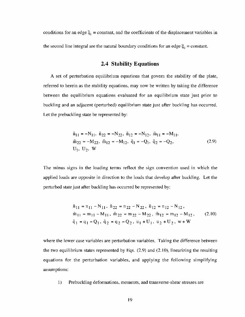
2.4 Stability Equations

A set of perturbation equilibrium equations that govern the stability of the plate,

referred to herein as the stability equations, may now be written by taking the difference

between the equilibrium equations evaluated for an equilibrium state just prior to

buckling and an adjacent (perturbed) equilibrium state just after buckling has occurred.

Let the prebuckling state be represented by:

fill =-Nll, fi22 =-N22, ill2 =-N12, liall =-Mll,

frizz =-M22, ffll2 =-M12, ql =-Q1, q2 =-Q2,

u1, u2, w

(2.9)

The minus signs in the loading terms reflect the sign convention used in which the

applied loads are opposite in direction to the loads that develop after buckling. Let the

perturbed state just after buckling has occurred be represented by:

fill =nll -Nil, fi22 =n22-N22, ill2 =n12-N12,

roll =mll -Mll, ff122 =m22-M22, fill2 =m12-M12,

ql =ql-Q1, q2 =qz-Q2, Ul +U1, u2 +U2, w+W

(2.10)

where the lower case variables are perturbation variables. Taking the difference between

the two equilibrium states represented by Eqs. (2.9) and (2.10), linearizing the resulting

equations for the perturbation variables, and applying the following simplifying

assumptions:

l) Prebuckling deformations, moments, and transverse-shear stresses are

19

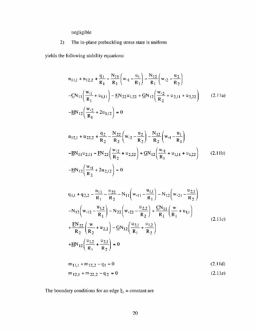
2)

negligible

The in-plane prebuckling stress state is uniform

yields the following stability equations:

nll,1 + n12,2 +ql Nll u_ _N__w

w,_-g _ /,_R1 R1

-_HN12(_12 +2u1,12) =0

(2.1 la)

+ n22, 2 + q2 N22 (n12,1R2 R2 w,2__2) _ N12 { w Ul

+ u 1,11 + u 1,22-__BNllU2,11 _ K2 _ R1

-HN12( w'l +2u2,12 ) = 0-- _R 2

(2.1 l b)

( _u1,1) ( _u2,1)rill n22 N11 W,ll -N12 w,21ql,1 + q2,2 R1 R2 R1 ) R2 )

( ( u22 cNll w+)_Ul,2]_N22 w,22_ +_ li __ Ul,1-N12 w,12 R1 ) R2 ) R1 _R1

w ) _, /u2,1 Ul,2 ]+ FN 22 (__ + u 2,2 +

R2 k R2 -_1"112(--_- 1 R2 ,/

+" {Ul'2 + U2'l] = 0I-tIN 12 _ R1 R2 )

(2.1 lc)

roll,1 + m12,2 -ql = 0

m12,1 + m22,2 - q2 = 0

(2.1 l d)

(2.11e)

The boundary conditions for an edge _1 = constant are

20

iSU 1 = 0

or

nll-CNll( ul'l +_1) + GN12u2,1 - HN12Ul, 2 = 0

i_U 2 = 0

or

n12--NllU2'l + GN12( ul'l +_-1)- _HN12( u2'2

iSw = 0

or

1- 11Iw1+U1 - 1 (=0

=0

(2.12a)

(2.12b)

(2.12c)

_)1 = 0 or mll = 0 (2.12d)

_)2 = 0 or m12 = 0 (2.12e)

As will be discussed in Chapter III, a sinusoidal variation of displacements and forces is

assumed in the _1 direction. Therefore, these boundary conditions are ignored herein.

The boundary conditions for an edge _2 = constant are

i_U 1 = 0

or

fi12 = n12 - ENzzUl,2 + GNlz(u2,2

6u 2 = 0

or

fi22 = n22-___N22(u2,2 +_-ff)

6w = 0

+__GN12Ul, 2 - HN12u2,1 = 0

=0

(2.13a)

(2.13b)

21

or

R1] R2]

i_l = 0 or m12 = 0

6_2=0 or m22=0

=0

(2.13c)

(2.13d)

(2.13e)

where the terms with a caret (^) are effective force quantities per unit length at an edge

_2 = constant. The effective forces, fi12,fi22, and q2 are equal to forces in the original

(undeformed) _1-, _2-, and _3-directions along the longitudinal edges of the plate

(_2=constant). Introduction of these force quantities facilitates the derivation of the

stiffness matrix in Chapter III which relates the forces along the longitudinal edges of the

plate in the original coordinate directions to the corresponding displacements along those

edges.

The first three stability equations given in Eqs. (2.11a) through (2.11c) are now

written in a simplified form using the definitions of the effective forces per unit length

given in Eqs. (2.13a) through (2.13c)

nll,1 + fi12,2 +ql Nll Ul _ ;w

W,l-gR1 R1

-CN11(_ll + u1,11)+__GN12u2,11-HN12u1,12 =0

(2.14a)

+ fi22,2 + q2 N22 (n12,1R2 R2

w,2-_2) - N12 (wR 2 _ '1-_11 )

.N11u211+ON12 w1) )+Ul,ll -HN12 +u2,12 =0

(2.14b)

22

( u1,1) ( u2,1)ql,1 +q2,2 nll fi22 N11 W,ll - _N12 w,21 -R1 R2 R1 ) R2 )

+CNl1( 1)+Ul,1R1

GN12u2,1 _HN12Ul,2+ -0

R1 R1

(2.14c)

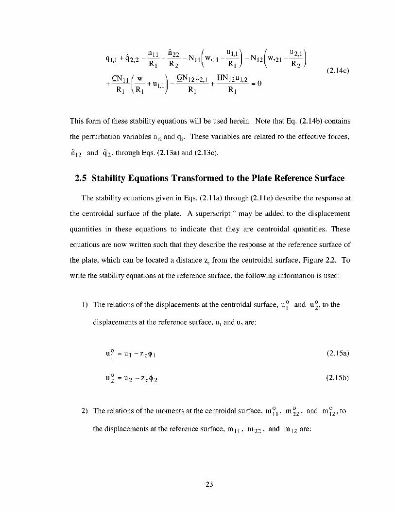
This form of these stability equations will be used herein. Note that Eq. (2.14b) contains

the perturbation variables n12 and q2. These variables are related to the effective forces,

fi12 and q2, through Eqs. (2.13a) and (2.13c).

2.5 Stability Equations Transformed to the Plate Reference Surface

The stability equations given in Eqs. (2.1 la) through (2.1 le) describe the response at

the centroidal surface of the plate. A superscript ° may be added to the displacement

quantities in these equations to indicate that they are centroidal quantities. These

equations are now written such that they describe the response at the reference surface of

the plate, which can be located a distance zc from the centroidal surface, Figure 22. To

write the stability equations at the reference surface, the following information is used:

o and o1) The relations of the displacements at the centroidal surface, u 1 u2, to the

displacements at the reference surface, u I and u 2 are:

O

u 1 = u 1 -Zc_ 1 (2.15a)

O

U2 = U2 - Zc_ 2 (2.15b)

2) o o and oThe relations of the moments at the centroidal surface, m 11 ' m 22 ' m 12' to

the displacements at the reference surface, mll, m22, and m12 are:

23

o (2.15c)roll =mll-zcnll

om22 = m22 - Zcn22 (2.15d)

om12 =ml2-zcnl2 (2.15e)

3) The following quantities do not vary with z:

Nll, N22, N12, n11, n22, n12, ql, q2, and w

4) The applied in-plane stresses, Nll , N=, and N12 act at the centroidal surface.

Substitution of Eqs. (2.15a) through (2.15e) into Eqs. (2.14a) through (2.14c) and Eqs.

(2.1 ld) and (2.1 le) yields the following equations

Ul --Zc@l-] - N12 (w+ ql Nil w, 1

nll,1 + fi12,2 R1 R1 R1 ] R1 _ ,2

+ Ul, 1 - Zcqbl + GN12[ u2 - Zcqb2 ],11,1

-__12[ul-Zc<],12=0

(2.16a)

+ fi22,2 + q2 N22 (w,2n12,1R2 R2

U 2 - Zc_) 2

R_ ) _ N_ (wR2 [ ,1

(u,- Zc<),,,+GN,,(w,, )_, R1 +[ ul -Zcq_l],ll

_I-IN 12 ( W'l )_,R2 +[u2-Zcq_2]12 =0

U 1 - Zc_) 1

(2.16b)

24

ul -_Z_c_l./ql,1 + q2,2 nll fi22 N11 w, 1

R1 R2 R1 ) ,1

u2 - Zcq_2 +__ +[ul_ Zcq_l] (2.16c)-_,_w,_ _7 ,, _, tU "

_N,_[u_-Zc<],,HN,_[u,-Zc<],___o+ +

R1 R1

mll,1 +ml2,2-Zc(nll,1 +n12,2)-ql--0 (2.16d)

m12,1 +m22,2-Zc(nl2,1 +n22,2)-q2 =0 (2.16e)

The natural boundary conditions are also rewritten after substitution of Eqs. (2.15a)

through (2.15e) into Eqs. (2.13a) through (2.13e). For an edge _2 = constant, the natural

boundary conditions become

(E w)12 = n 12 - __EN22[U1 - Zc* 1]2 + G N 12 u2 - Zc*2 ],2 + _2

(E---HN12 Ul -Zc*l],l + = 0

(2.17a)

n22 = n22 - FN22([u2 - Zc_)2],2 + + ---GN12[u1 - Zc*l ]2

-L_]12[ u2 - Zc*2 ],1 = 0

(2.17b)

2=q2Ni2(wiEuizc 11:I Eu2zc 21:+ 7,-7 )- _= w_+ _,7 .):o (2.17c)

m12 - Zcnl2 = 0 (2.17d)

25

m22- Zcn22= 0 (2.17e)

The last two stability equations, Eqs. (2.16d) and (2.16e), are now rewritten by

substitutingexpressionsfor the quantities(n 11,1+ n12,2) and (n 12,1+ n22,2)that can

be obtainedusing Eqs. (2.16a) and (2.16b), respectively,and the definitions for the

effective forcesper unit length, Eqs. (2.17a)through (2.17c). The definitions for the

effectiveforcesareneededsincethetermsn12andn22thatappearin thetwo abovearethe

perturbationvalues,not theeffective forces. Substitutionof theexpressionsfor thetwo

quantitiesaboveinto Eqs. (2.16d) and(2.16e),respectively,yields the final form of the

lasttwo stability equations

[ (u,_zc_,)mll,1 +m12,2-ql +zc ql Nil w, 1R1 R1 R1

N'_,(w,_u_-zc_)___N,(_,_+u,,,w-Zc_,),1

-EN_(u_-Zc,_t_ +C_N_(w'_R_ +[u_- Zc_,_],_

( w'2 2[u 1-zcq_l],12)] =0

(2.18a)

m12,1 + m22,2 - q2 + Zc u2 - Zcq_2.]q2 N22 w, 2R2 R2 R2 )

N12 (w,1 Ul -Zcq_ 1R2, _,i )-_BNll(Ua-Zc*2)ll

__Naa(W,_ ) (w,,_R 2 +[u2-Zcqb2],2 2 +GN12 +[Ul-Zcqbl],l 1- _R I

+i-zc_l_,aal-.NlalWl_,_2+_Eo2-Zc_2_,121]:o

(2.18b)

26

The stability equations in the form given in Eqs. (2.16a) through (2.16c) and Eqs. (2.18a)

and (2.18b) are those implemented into the VICONOPT code.

2.6 Constitutive Relations

The present analysis allows for generally laminated composite materials. The

geometry of a general, curved laminate is given in Figure 2.3. As shown in the figure,

the number of layers in the laminate is n1, and the width of the laminate is b. The radius

of curvature of the _2-axis, R 2 is shown in the figure as well.. The radius of curvature of

the _l-axis, R1 is not shown; however, its direction may be inferred from that of R2. The

lamina coordinate system is the (_v, _2,, _3) system and the laminate coordinate system is

the (_, _2, _3) system. The lamina coordinate system is aligned with the principal

material direction of the lamina, and the laminate coordinate system is aligned with the

principal geometric directions of the laminate. The coordinate system for the kth lamina

is oriented at an angle 0 k with respect to the laminate coordinate system. The stress-strain

relations in the lamina coordinate system for a lamina of orthotropic material in a state of

plane stress are

t 11tr 1101t 11]°22 °o2 0 221:12' Q66 12

(2.19)

where the [Q] matrix is referred to as the reduced stiffness matrix for the lamina and is

defined in [45] in terms of the elastic engineering constants of the lamina. These

relations may be written in the laminate coordinate system by use of transformation

matrices as defined in [45]. The transformed relations are

27

t+11ti+11012 161i11to===IQ_,=_==_=6i_==1:12 [q16 Q26 Q66 [Y12

(2.20)

where the [Q] matrix is the reduced transformed stiffness matrix for the lamina. Both of

Eqs. (2.19) and (2.20) may be thought of as stress-strain relations for the kth lamina in a

multi-layer laminate. Therefore, Eq. (2.20) may be written as

{O'}k = [Q]k {e}k (2.21)

The constitutive relations for a thin, elastic laminated composite shell may now be

defined as

-N11

N22

N12

Mll

M22

M12

All A12 A16

A12 A22 A26

A16 A26 A66

Bll B12 B16

B12 B22 B26

B16 B26 B66

Bll B12 B16

B12 B22 B26

B16 B26 B66

Dll D12 D16

D12 D22 D26

D16 D26 D66

Ell

E 22

Y12

1(11

1( 22

1(12

(2.22)

where the resultant forces and moments acting

respectively, are defined as

tN11t Zk +11tN22 = _ Zkfll°22 d_3N12 k=l - ["g12

on the laminate, {N} and {M},

(2.23)

[_"I z_[°"lM22 = _ ZkfllO22_ _3 d_3M12 k=l - ['g12 |

(2.24)

28

wheren_is the total numberof layersin the laminate. The extensional,coupling, and

bendingstiffnessmatrices,A, B, andD, respectively,aredefinedas

(A, B, D)= ni Zk 3 ) d_3 (2.25)k=l Zk_ 1

The analysis in VICONOPT allows for laminates with fully populated A, B, and D

matrices.

The constitutive relations for transverse shear used in VICONOPT are those

presented by Cohen in [44]. The constitutive relations for transverse shear are written in

inverted form as

{ 13}:rkllk12]fql}23 [k12 k22 q2(2.26)

where [k] is a symmetric 2-by-2 transverse shear compliance matrix whose terms are

defined in [44]. The terms of the [k] matrix were derived for general, anisotropic, multi-

layered composite shells and they are a generalization of results for a shell with a

homogeneous wall for which the transverse shear correction factor for the shear stiffness

is 5/6. The procedure used in [44] for obtaining the terms of the [k] matrix follows.

Statically correct expressions of in-plane stresses and transverse-shear stresses were

derived in terms of the transverse-shear stress resultants and arbitrary constants that were

interpreted by Cohen as redundant "forces". The expressions for in-plane stresses were

obtained using the constitutive relations given in Eq. (2.22) and linear distribution of in-

plane strains through the wall thickness. The expressions of transverse-shear stresses

were obtained by integrating in the _3-direction the three-dimensional equilibrium

equations. The transverse-shear stress resultants were then used to derive an expression

of the volumetric density of the transverse-shear strain energy. A statically correct

29

expressionof theareadensityof the transverse-shearstrainenergywasthenobtainedby

integratingin the_3-directionthis volumetric density. Thetransverse-shearconstitutive

relationsgivenin Eq. (2.26)werethenderivedby applyingCastigliano'stheoremof least

work [46] by minimizing the areadensity of the transverse-shearstrain energywith

respectto theredundantforcesmentionedpreviously.

30

CHAPTER III

IMPLEMENTATION INTO VICONOPT

In this chapter, the implementation of the present theory into the VICONOPT code is

described. Additional simplifications made to the theory are described first. A

discussion of the use of the transverse-shear strain, _'13, as a fundamental displacement

variable in the problem to maintain continuity of rotations at plate junctions is then

presented. The derivation of an expression for the curved-plate stiffness matrix is

described. The terms of matrices that are needed to calculate this stiffness matrix were

obtained using MATHEMATICA [40], and they are presented in Appendix A. The terms

for both CPT and SDPT are presented, and the terms that result from the inclusion of

direct in-plane transverse and in-plane shear loads in the in-plane stability equations are

specified. As stated previously, the implementation of the curved-plate theory into

VICONOPT follows very closely the method presented in Reference [2]. Therefore, the

following discussion is necessarily similar to that presented in that reference.

3.1 Simplifications to the Theory

Before proceeding with the derivation of the curved-plate stiffness matrix, a

discussion of several simplifications to be implemented is presented. First, the theory

implemented into the VICONOPT code considers structures that are prismatic in the

longitudinal direction. Therefore, for the curved plates being considered in the present

report, the radius of curvature in the longitudinal direction, R1, is infinite; and any terms

1involving the quantity -- are zero. Although these terms are set equal to zero for the

R1

calculation of the terms of the stiffness matrix, they are retained for completeness in the

31

theorypresentedin this chapter. Another simplification to the theory involves limiting

the capability to locate the referencesurfacea distancezcfrom the centroidal surface.

This capability hasonly beenimplementedfor thecasewheretheeffectsof N= andN12

loadsin the in-planestability equationsareneglected.Theexpressionsfor the stiffness

termsthat resultwhenN= andN12areincludedin the in-planestability equationsand zc

is non-zero are prohibitively long. Therefore, in the derivation to follow, only the

following two casesarepresented:

1) N= and N12are included in the in-plane stability equationsand z_is zero (i.e.,

referencesurfaceis coincidentwith thecentroidalsurface);and,

2) N= andN12areneglectedin the in-planestability equationsand z_is non-zero(i.e.,

referencesurfacemaybetranslatedfrom thecentroidalsurface).

3.2 Continuity of Rotations at a Plate Junction

One important issue to be addressed in the analysis of plate assemblies is the

continuity of rotations at a plate junction. The original VIPASA code is based upon CPT,

and the theory only treats four degrees of freedom (DOF) at a longitudinal plate edge.

These DOF are the three displacement quantities, u1, u2, and w, and a rotation about the

_1 -axis, _)2. Maintaining continuity of these DOF at a typical plate junction is very

straightforward. However, when SDPT is considered, there are five DOF at a

longitudinal plate edge. These DOF are the four from CPT as well as an additional

rotation, _)1, that results from the inclusion of transverse-shear deformation. Another

problem that must be addressed is that when two plates are joined together such that one

is rotated at an arbitrary angle, 0, to the other, rotations about the normals to the

centroidal surfaces of the two plates must be included to satisfy continuity of rotations.

This rotation, %, is not accounted for in the present plate theory. The procedure used in

32

VICONOPT to maintain continuity of rotations follows that used by Cohen in [47]. This

procedure introduces the shear strain, _'13,as a fundamental displacement variable instead

of the rotation, '1. The justification for using this approach is described subsequently.

The displacements and rotations at a typical plate junction are shown in Figure 3.1.

The two plates, numbered 1 and 2, are shown viewed along the 1-axis, and it is obvious

that the u 1 displacements are easily matched regardless of the orientation of plate 2. The

displacements and rotations for which continuity must be maintained are u2, w, '1, and %.

Upon inspection of Figure 3. l(a), the following expressions for coplanar plates (0 = 0)

may be written as

u 1 = u_ (3.1a)

w 1 = w 2 (3.1b)

,1 n =,2 (3.1d)

where the superscripts 1 and 2 refer to the plate numbers. Similarly, upon inspection of

Figure 3. l(b), the following expressions for 0 = +90 ° may be written as

u 1 = w 2 (3.2a)

w 1 _u 2= 2 (3.2b)

,11 = _,2 (3.2c)

,1 n =,2 (3.2d)

33

Finally, uponinspectionof Figure 3.1(c),the following expressionsfor arbitrary0 may

bewrittenas

u1 = u2 cosO+ w2sinO (3.3a)

w1 = w2cosO- u2sinO (3.3b)

911=92 cosO- _2 sinO (3.3c)

91n = 9 2 cos0 + 9 2 sin0 (3.3d)

The rotation about the normal of a line element originally directed along the _l-axis is

shown in [48] to be

0u 29n - (3.4)

Using this definition, Eqs. (3.3c) and (3.3d) are written as

29] = 9 2 COS{)- U2,1 sinO (3.5a)

1 2 + 912 sinU2,1 = U2,1 COS6 19 (3.5b)

Using Eqs. (3.3a) and (3.3b) and the definition for _t13, Eq. (2.2d), the previous two

equations may be written as

7 113 = cosO 7 213 (3.6a)

0 = -sinO 7 213 (3.6b)

34

The results shown in Eqs. (3.6a) and (3.6b) indicate that for plates that are not

coplanar (i.e., one plate oriented at an arbitrary angle, 0, to the other), the shear strain, 713,

must be set equal to zero for each plate to maintain continuity of rotations. Therefore, if

713 is made a fundamental displacement quantity instead of _h, the shear strain can be set

equal to zero by simply striking out the appropriate rows and columns in the overall

stiffness matrix. Performing this operation reduces the stiffness matrix to the same size

as that for CPT. The VICONOPT code utilizes this procedure for plates that are not

coplanar. For plates that are coplanar, i.e., 0 = 0, the shear strain in plate 1 is equal to

that in plate 2. The VICONOPT code handles this situation by creating a substructure

using the two plates with all DOF present and eliminating the extra DOF before assembly

into the final stiffness matrix.

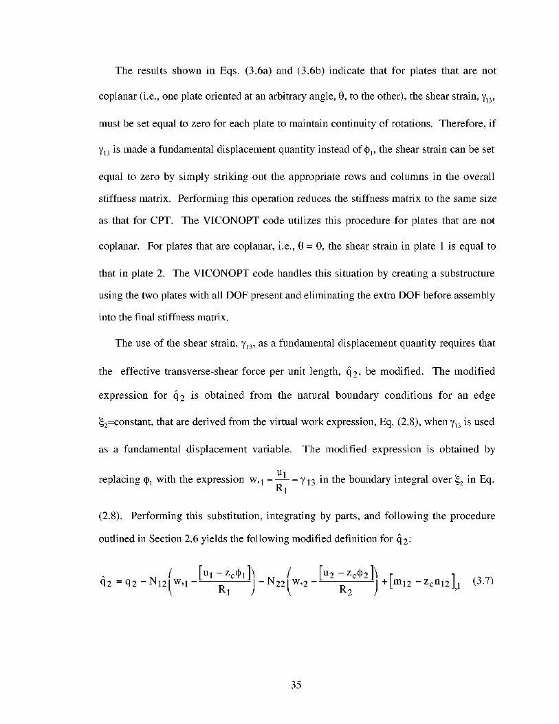
The use of the shear strain, 713, as a fundamental displacement quantity requires that

the effective transverse-shear force per unit length, q2, be modified. The modified

expression for q2 is obtained from the natural boundary conditions for an edge

_2=constant, that are derived from the virtual work expression, Eq. (2.8), when 713 is used

as a fundamental displacement variable.

replacing _)1 with the expression w, 1 ----Ul

R1

The modified expression is obtained by

_' 13 in the boundary integral over _2 in Eq.

(2.8). Performing this substitution, integrating by parts, and following the procedure

outlined in Section 2.6 yields the following modified definition for q2:

{q2 =q2-N12_w,1 [Ul -Zc_l])p'l )- N22( w'2

[u2- Zc,2]))R2

+[ m12 -Zcnl2],l (3.7)

35

Thedefinition for q2 given in Eq. (3.7) replaces that given in Eq. (2.17c). Note that the

term m12,1 which appears in the Kirchhoff shear term of CPT is also present for the case

of SDPT when _'13,is used as a fundamental displacement quantity.

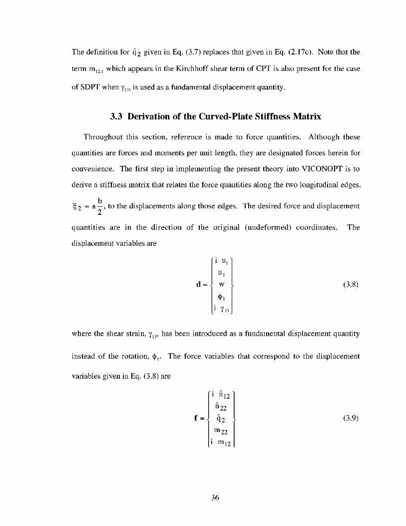
3.3 Derivation of the Curved-Plate Stiffness Matrix

Throughout this section, reference is made to force quantities. Although these

quantities are forces and moments per unit length, they are designated forces herein for

convenience. The first step in implementing the present theory into VICONOPT is to

derive a stiffness matrix that relates the force quantities along the two longitudinal edges,

b_- to the displacements along those edges. The desired force and displacement_2 =+2'

quantities are in the direction of the original (undeformed) coordinates. The

displacement variables are

i u 1

U2

d= w

,2

i _'13

(3.8)

where the shear strain, _'_3, has been introduced as a fundamental displacement quantity

instead of the rotation, %. The force variables that correspond to the displacement

variables given in Eq. (3.8) are

"i ill2^

n22^

q2

m22

i m12

(3.9)

36

Note that theeffective forcesat theboundaries,definedby Eqs.(2.17a)and(2.17b)and

Eq. (3.7),arebeingusedastheforcequantitiessince,asdiscussedin ChapterII, theyare

equalto theforcesin thedirectionof theoriginal (undeformed)coordinates.

Theproblemmaynow be reducedto ordinarydifferential equationsin y by assuming

that the responseof the plate in the longitudinal _l-direction varies sinusoidally.

Therefore,if thedisplacementsandforcesin theplatearenow consideredto befunctions

of _2,thevariablesof Eqs.(3.8)and(3.9)maybewrittenas

where

i = _1 )z(_ 2 ) (3.10)Z(_I,_ 2 )= exp )v

and )v is the half-wavelength of the response in the _l-direction. Since a sinusoidal

variation in the _l-direction is assumed, the vector z will involve the amplitudes of the

displacement and force quantities. The imaginary number, i, has been used in Eqs. (3.8)

and (3.9) to account for the spatial phase shift that occurs between the perturbation forces

and displacements which occur at the edges of the plates during buckling for orthotropic

plates without shear loading and to result in real plate stiffnesses when using the

exponential expression of Eq. (3.10).

The next step in the derivation is to express all unknowns in terms of z. A partially

inverted form of the constitutive relations, Eq. (2.22), is used to express the required

quantities as functions of the fundamental variables in d and f or terms that may be

derived from the fundamental variables. The partially inverted constitutive relations are

37

nll] [ hll h12 h13 h14 h15 h16 t;ll

t;22 ] ] -h12 h22 h23 h24 h25 h26 n22

_12 _ = /-hl3 h2____3 h3____3 h3___44 h3___55h3____66nl_____2

mll / / h14 -h24 -h34 h44 h45 h46 ' Kll

22| l-his h2s h35 -h45 h55 h56 m22

_:12 J I-hi6 h26 h36 -h46 h56 h66 m12

_'21

(3.11)

where the linear portion of _11 from Eq. (2.2a) is used

W

t;ll =Ul, 1 +--R1

The variables _ql and 91 were defined in Section 2.2 of Chapter II. The constants h_j in

the first portion of Eq. (3.11) are calculated from the A, B, and D matrices defined in Eq.

(2.25). The constants h77, h78, and h88 are shear stiffness terms and are calculated using

the theory presented in [44].

Another requirement of the present derivation is to express the relationship between

q2 and q2 without any _2-derivatives. This expression is

{\ [Ul- Zc_)l])R1 + N22(q)2- h7871)+[m12- Zcnl2],lq2 + N12 [w,1

(3.12)q2 = 1- N22h88

As with the stability equations, only the linear portion of the strain-displacement

relations are considered in the present derivation

38

Y12 = Ul,2 + U2,1 (3.13a)

w1322 = u2, 2 +-- (3.13b)

R2

u223 = w,2 --- - 92 (3.13c)

R2

1_22 = -92,2

= +%1)

(3.13d)

(3.13e)

The expression for r_12can be re-written after substituting expressions obtained for 91 and

92 from Eqs. (2.5a) and (2.5b) and using the linear portion of 1312

R2 U2+292 ] +131----2-2+Y1,2,1 R1

(3.13f)

Using Eqs. (3.11) and (3.12), the strain displacement equations, Eqs. (3.13a) through

(3.13d) and (3.13f) and the equations, Eqs. (2.16a) through (2.16c) and (2.18a) and

(2.18b) are written in terms of the elements of z as

T z'=Pz or z'=T _ Pz (3.14)

where a prime denotes differentiation with respect to _2. The square matrix T appears in

the present study as a result of the inclusion of the effects of N= and N12 in the in-plane

equilibrium equations. This matrix was shown to be the identity matrix when these terms

were neglected in [2]. The presence of off-diagonal terms in this matrix is a fundamental

difference between the present theory and that presented in [2].

The elements of z are now assumed to be given by

39

i [5 _2) (3.15)zj = cj exp b

where [5 is a characteristic root of the differential equation. The number of values of [5 is

equal to the order of the differential equation system. Substitution of Eq. (3.15) into Eq.

(3.14) results in the following equation

where

(R - [51) c = 0 (3.16a)

R = bT-1p (3.16b)

and I is the identity matrix. The vector c consists of the cj of Eq. (3.15). The matrix R is

obtained by premultiplying P by T 1. The eigenvalues of the matrix R are the

characteristic roots of the differential equation. This matrix is not symmetric; however, it

can be made real by multiplication or division of appropriate rows and columns by the

imaginary number, i. The elements of the matrices T and P are given in Appendix A for

both SDPT and CPT.

For each eigenvalue of R, there exists an eigenvector, e. A matrix C may be defined

with columns as the eigenvectors, e, the upper half of each column, denoted a, will be

associated with displacements, and the lower half, denoted b, will be associated with

forces. The form of C is therefore

a a 2 . . . ajC= bl b 2 . . . bj(3.17)

The next step in the derivation is to write the amplitudes of the displacements and forces

at the two edges of the plate. Quantities evaluated at _2 =--- are identified with a

40

bsuperscript1 andquantitiesevaluatedat _2 -- +- are identified with a superscript 2 as

2

follows:

d! = N (-i 13kJ _ ajkr k exp

k=l _ 2(3.18a)

J = _ ajkr k exp (3.18b)k=l

N (-i 13kf = _ bjkr kexpk=l 2

(3.18c)

f2 = E bjkrkexp (3.18d)k=l

where the rk are constants determined from the edge values and N is the order of the

differential equation. Equations (3.18a)-(3.18d) may be written in matrix form as

{"'}d2 =Er

{f'}f2 =Fr

(3.19)

(3.20)

Eliminating r from Eqs. (3.19) and (3.20) yields

(3.21)

where K is the stiffness matrix given by

K = F E "1 (3.22)

As for the case of CPT, K is real and symmetric for orthotropic plates without in-

plane shear loading, and it is Hermitian otherwise. Reference [2] presents a discussion of

41

techniquesusedto ensurethat accuratenumericalresultsfor K are obtainedfrom Eq.

(3.22).

3.4 The Wittrick-Williams Eigenvalue Algorithm

A brief discussion of the analysis procedure used in VICONOPT is in order. As

previously mentioned, VICONOPT uses a specialized algorithm for determining any

natural frequency or buckling load for any given wavelength [29]. The development of

this algorithm was necessary because the complex stiffnesses defined in the previous

section are transcendental functions of the load factor and half wavelength of the

buckling modes of the structure. The eigenvalue problem for determining natural

frequencies and buckling load factors is therefore transcendental.

The iterative analysis procedure used in VICONOPT is described in [36]. For this

procedure, the plate stiffnesses for a given wavelength are evaluated at a series of trial

values of the eigenvalue being determined until convergence is attained. This eigenvalue

is either the load factor for buckling or the natural frequency for vibration, and it is

different than the eigenvalues of the R matrix of Eq. (3.16b). Unless otherwise specified

by the user, the default initial trial value used in the VICONOPT code is one. For each

trial value of the eigenvalue considered, the analysis requires the plate stiffnesses as well

as the number of eigenvalues that lie below the trial value for the entire plate assembly

assuming the longitudinal edges of each individual to be clamped. A complete

description of the eigenvalue algorithm is given in [28]. Determining the number of

eigenvalues exceeded by a plate with clamped edges is very difficult except for very

specialized cases. Therefore, the procedure developed in [28] is used. This procedure

subdivides each plate into sub-elements with a small enough width such that none of the

eigenvalues of the sub-elements with clamped edges lie below the trial value. A sub-

elements is then used as a substructure and is repeatedly doubled until the original plate

element is obtained. Using a simple procedure at each doubling step [29], the number of

42

eigenvalues that lie below the trial value for the complete plate is returned. This

procedure is repeated for each plate in the assembly. Using this information and other

information obtained from the stiffness matrix of the entire assembly, the total number of

eigenvalues for the entire plate assembly that lie below the trial value is obtained. An

iterative procedure is then used to refine the trial value until the desired eigenvalue is

calculated to within the accuracy required.

One important piece of information required for the analysis procedure described

herein is the number of subdivisions required for each plate. As seen in Appendix A, all

of the terms of the R matrix are proportional to the plate width, b. Therefore, all of the

eigenvalues of R are proportional to b. Furthermore, it is important to note that an

eigenvalue equal to _ corresponds to buckling or vibration with simply supported

longitudinal edges. By successively halving the value for b until all the real eigenvalues

of R are less than _, a value for the width of the sub-elements for which no eigenvalues

lie below the eigenvalue for simply supported edges is determined. This width also

guarantees that no eigenvalues for the sub-elements lie below the eigenvalue for clamped

edges. This width is that used in the iterative analysis procedure described previously.

43

CHAPTER IV

NUMERICAL RESULTS

In this chapter, numerical results are presented using the newly implemented curved-

plate analysis capability in VICONOPT. Results from several example problems are

presented to verify the results obtained with this new capability. A convergence study

using the segmented-plate approach in VICONOPT is performed for an isotropic

cylindrical shell subjected to uniaxial compression to identify a suitable number of

segments to be used when comparing results. Results comparing the computational effort

required by the new analysis to that of the analysis currently in the VICONOPT program

are also presented for this example. Comparisons of results for several curved plates

analyzed in Ref. [32] are then made. The effects of including terms related to in-plane

transverse loads in the in-plane stability equations are examined using a long cylindrical

tube subjected to in-plane transverse loading. Finally, the curved-plate analysis is used to

conduct a design-optimization study of a honeycomb-sandwich cylindrical shell

subjected to uniaxial compression. Comparisons of analyses using both physical and

tensorial strain measures are made for selected examples, and, where appropriate, results

using CPT and SDPT are compared.

4.1 Convergence of the Segmented-Plate Approach

The convergence of results using the segmented-plate approach in VICONOPT is

examined for the case of an aluminum cylindrical shell subjected to uniaxial

compression, see Figure 4.1. The values of the material properties used for this example

are E = 10.0 x 106 psi and v12 = 0.33. The wall thickness, t, is 0.1 in., and the radius, R2 is

60 in. As shown in Reference [49], the critical value for the stress resultant, Nllcr, for

the axisymmetric buckling of a long isotropic cylindrical shell is

44

Et 2

Nllcr = R2_/3(1 v22)-1019.354lb/in._ (4.1)

For v12 = 0.33, the critical half wavelength, )_cr, for axisymmetric buckling is shown in

[49] to be

f R2t 2)_cr _ /= in. 4.2,

Results illustrating the convergence of the VICONOPT segmented-plate results for

Nllcr as a function of the number of segments used to approximate the cylinder are

shown in Figure 4.2. In this figure, the results of the segmented-plate analysis are shown

as the solid curve. The theoretical value obtained from Reference [49] is shown as the

dashed horizontal line. The value obtained using the present curved-plate analysis with

two curved-plate elements is shown as the open symbol. All results in this figure are

calculated for the value of )_cr given in Eq. (4.2). The VICONOPT results presented in

this figure are obtained using CPT with tensorial strain measures. As shown in Figure

4.2, the segmented-plate results converge to the theoretical value when 120 segments are

used. Therefore, to ensure that converged results are obtained when the segmented-plate

approach is used to analyze the remaining example problems, sixty segments will be used

when analyzing curved plates with an included angle of 180 degrees or less, and 120

segments will be used when analyzing full cylinders.

This example problem is also used to study the computational requirements of the

new curved-plate analysis in relation to the segmented-plate approach. A plot of

normalized CPU time as a function of the number of plate segments used in the

approximation is shown in Figure 4.3 for the segmented-plate analysis using either CPT

or SDPT. The normalized CPU time shown in this figure is the CPU time required for

45

the segmented-plateanalysesnormalizedwith respectto the CPUtime requiredfor the

curved-plateanalysisusingtwo curved-plateelements.The horizontaldashedline is at a

normalizedCPU time of 1.0, and it representsthe curved-plateanalysis results. As

shown in the figure, to achieve convergencewith 120 flat-plate segmentsrequires

approximately3.5 timesand 16.7timesasmuchCPUtime asthecurved-plateanalysis

for CPTand SDPT,respectively. (For theanalysisusingSDPT,G12= G13= G23).One

considerationto noteat this time is that the segmented-plateanalysisin VICONOPT is

implementedto handlethegeneralcaseof variablegeometry,stiffnessandloadingin the

_2-direction.This approachis thereforenot ascomputationallyefficient asit couldbefor

thecaseof constantcurvature,stiffness,and loadingin that direction (as is the casefor

the curved-plateanalysis). Oneapproachto determiningthe additional computational

efficiency that may be obtainedwith the segmented-plateanalysisinvolves defining a

single,small flat plate that is repeatedlydoubledusingthe substructuringcapability in

VICONOPT until the curved-platesegmentis obtained. This techniqueis referredto

hereinas 'doubling'. Resultsrelating the computationaleffort of this approachto the

curved-plateanalysisindicate thatfurther reductionin thecomputationaleffort required

for the segmented-plateanalysiscanbeobtainedusingthis technique.This result occurs

becausethe in-plane and out-plane equationsare uncoupled in the segmented-plate

analysis,andanalyticalexpressionsfor the platestiffnessescanbeused. However,this

approachis currently not automatedin the VICONOPT code,anda separate'doubling'

effort would have to be madefor every curved-platesegmentin any given analytical

model.

4.2 Buckling of Curved Plates With Widely Varying Curvatures

The example problems presented in the next two sections are taken from Ref. [32],

and they are used to verify the results obtained using the new curved-plate analysis in

VICONOPT. The positive sense of the applied in-plane loadings to be considered in all

46

of the following examplesis givenin Figure4.4. Thefirst exampleproblemconsidered

studiesthebuckling of a symmetricallylaminatedcurvedplatewith clampedlongitudinal

edgesasa function of thecurvatureof theplate. The geometryof the plateis shownin

Figure 4.5. As shown in the figure, the plate is constructedfrom symmetrically

laminatedboron/epoxyplieswith a [0/90/+45]slayup. To allow for direct comparisonof

resultswith thosepresentedin [32], the SI units are usedfor this exampleand the

examplein the following section. The material propertiesfor a boron/epoxyply are

givenin Table1.

Thefollowing loadingsareconsideredfor this exampleproblem:Nil only, N= only,

N12only, andcombinedNil = N= = N12.The buckling of this plate subjectto thesefour

different loadingswas investigatedwhile varying the valueof the curvatureparameter,

b2--, from 1to 1000. Thevaluesof b, R2,and[_usedfor theseanalysesaresummarizedR2t

in Table 2. Both physical and tensorial strainsare used with the new curved-plate

analysis,while physical strainsonly are usedfor the segmented-plateanalysis. The

analysisof [32] usesphysicalstrains.All analysisresultspresentedin this sectionarefor

CPT. Thetermsinvolving N= andN12areincludedin the in-planestability equationsfor

all analyses.Theresultsof this studyarepresentedin Table3 for Nil loading,in Table4

for N= loading, in Table 5 for N12loading,andin Table6 for combinedNil = Nz2= N12

loading. The critical values of the stressresultantspresentedin these tables were

calculatedusing for the values of -- given in the tables. Thesevalues of -- wereb b

presentedin Reference[32]. The critical valuesof thesestressresultantsarealsoplotted

asa function of the curvatureparameterin Figure 4.6 throughFigure 4.9,respectively.

As shownin thesetables,the presentanalysiscomparesvery well with that presentedin

[32] and with the segmented-plateanalysisfor widely varying valuesof the curvature

47

parameter. As shownin Tables3 - 6, thereis no appreciabledifferencein the results

obtainedusingphysicalandtensorialstrains.

4.3 Buckling of an Unsymmetrically Laminated Curved Plate

This example problem includes the effect of bending-stretching coupling and shear-

extension coupling on the buckling of an unsymmetrically laminated curved plate with

simply supported longitudinal edges. The geometry of the curved plate is shown in

Figure 4.10. As shown in the figure, the laminate being studied consists of a 0.0508-cm.-

thick layer of 2024 aluminum that is reinforced on the inner surface with pairs of -+45_

boron/epoxy plies. The material properties for 2024 aluminum are given in Table 1. For

this example, the number of pairs of _+45° boron/epoxy plies is increased from one to

seven. The analyses used for this example are identical to those used for the previous

example. The critical values for buckling of the stress resultants Nil and N12 are

presented in Tables 7 and 8, respectively. These values are also plotted as a function of

the number of boron/epoxy plies used in the laminate in Figure 4.11 and Figure 4.12,

respectively. The agreement between all the analyses is very good. As with the previous

example, there is no appreciable difference in the results obtained using physical and

tensorial strains. Results were also computed using SDPT. However, for the case of

seven pairs of pairs of _+45° boron/epoxy plies, the R/t ratio is still approximately 300,

and the effects of transverse-shear deformation are minimal. Therefore, as expected, the

critical values for buckling of the stress resultants Nil and N12 were slightly less than

those for CPT, but the differences were less than 0.2 percent. With regards to the CPU

time requirements for this example, the segmented-plate analysis using SDPT required

approximately 35 times as much CPU time as the curved-plate analysis for the case of 14

boron/epoxy plies. Furthermore, the results obtained using the 'doubling' approach

described in Section 4.1 indicate that the computational efficiencies offered by that

approach were not realized for this example problem. This result occurs because the

48

coupling that occurs due to the unsymmetric laminate prevents the in-plane and out-of-

plane equations from being uncoupled, and the same numerical approach for calculating

the plate stiffnesses as that used for the curved-plate analysis must be used.

4.4 Effect of N= Terms in the In-Plane Stability Equations

As stated previously, the original segmented-plate analysis in the VICONOPT code

neglects the effects of the terms involving N= and N12 in the in-plane stability equations.

This example problem illustrates the effect these terms may have on the buckling of an

isotropic (aluminum) long cylindrical tube subjected to uniform external pressure. The

material properties in English units for aluminum are given in Table 9. The geometry of

this example problem is shown in Figure 4.13. As shown in the figure, only half of the

tube is modeled since the buckling mode being studied is symmetric (i.e., two full waves

in the circumferential direction). The pressure load is modeled as an applied N22 hoop

loading. The value of the external pressure that would generate this hoop load is obtained

from the following expression [49]

N22p - (4.3)

R2

Simitses [50] presents a detailed discussion of the buckling of a thin circular ring

uniformly compressed by external pressure. When considering the behavior of the

pressure load as the ring buckles, Simitses describes three possible cases. In Case 1, the

pressure load is assumed to remain normal to the deflected surface. This loading is

referred to as a live pressure load. In Case 2, the pressure load is assumed to remain

parallel to its original direction. This loading is referred to as a dead pressure load. In

Case 3, the pressure load is assumed to always be directed toward the center of curvature

of the ring. This loading is referred to as a centrally directed pressure load. Only Cases 1

and 2 will be discussed in the present report.

49

In Reference [50], Simitses presents in-plane and out-of-plane stability equations for

the thin circular ring which may be rewritten in the notation used in the present report as

n22,2 R2 -Pcr w,2- -P2 =0(4.4)

n22 (R2w,22 -u2,2) P3 0 (4.5)q2,2 R2 Pcr - =

where P2 and P3 are the perturbation values of the applied pressure load in the buckled

state in the _2- and _3-directions, respectively. For the case of a live pressure load in

which the applied pressure is assumed to remain normal to the deflected surface, Pz and

P3 are (for small deformations)

(P2 =-Pcr w,2- and P3 = 0 (4.6)

For the case of a dead pressure load in which the applied pressure is assumed to remain

parallel to its original direction, P2 and P3 are

P2 = 0 and P3 = 0 (4.7)

Substituting Eqs. (4.3) and (4.6) into Eqs. (4.4) and (4.5), yields the following stability

equations for the case of live pressure loading:

+ q___m2= 0 (4.8)n22,2 R2

u2,2 ]n22 NZZcr w,22 - = 0 (4.9)q2,2 R2 R2 ]

50

SubstitutingEqs. (4.3) and (4.7) into Eqs. (4.4) and(4.5), yields the following stability

equationsfor thecaseof deadpressureloading:

n22,2-t q2 N22cr w,2- = 0R2 R2

(4.10)

u2,2]n22 N22cr w,22- = 0q2,2 R2 R2 )

(4.11)

For live pressure, the critical value of pressure is shown in [50] to be

Therefore,

3EI

Pcr - R_,2 (4.12)

3EI

NZZcr - R92 (4.13)

For dead pressure, the critical value of pressure is shown in [50] to be

4EI

Pcr R3(4.14)

Therefore,

4EI

N22cr- R2 (4.15)

51

As discussedin Reference[49], resultsfor the caseof a long cylindrical tubeuniformly

compressedby externalpressure,may beobtainedby consideringan elementalring of

unit width and using Eqs. (4.12) through (4.15) with E replaced by E/(1-v2) and I

replacedby t3/12.

External pressureloads are not included in the present analysis. However, an

equivalentN22loadingmay becalculatedusingEq. (4.3). Thepresentanalysistreatsthe

applied loadsasdeadloadssinceno effort is madeto modify the applied loadsas the

plate deforms. The stability equationsin the _2and _3directions, Eqs. (2.11b) and

(2.1lc) for thepresentanalysisarewritten for a thincircular ring subjectedto N22loading

by ignoring any terms that involve N12,_1, or derivativeswith respectto _. These

equationsare

- - + u2,22 = 0n22,2-t Rzq2 NZZR2w,2 _FN22_R2 (4.16)

u2,2.]+ -FN22n22 N22 w,22q2,2 R2 R2 ] R2 w )-- + U2, 2 = 0 (4.17)

R2

Comparing Eqs. (4.9), (4.11), and (4.17), reveals that if physical strains are used in the

present analysis (i.e., F = 0), the out-of-plane stability equation is identical to that given

by Simitses for both live and dead pressure loads. Furthermore, the in-plane stability

equation for the live pressure load case is recovered by the present analysis if the N22

term is neglected in Eq. (4.16). The dead pressure load case is seen to be recovered when

the N22 term is included in Eq. (4.16). Comparing Eqs. (4.6), (4.7), and (4.16), shows that

52

for the case of physical strains, the remaining term involving N= is actually equivalent to

the component of a live pressure load in the _2 direction (see Eq. (4.6)).

Buckling results for this example are presented in Table 10. The VICONOPT results

presented in this table are for physical strains. As previously discussed, the VICONOPT

result when the N= term is neglected in the in-plane stability equation corresponds to the

case of live pressure load, and the VICONOPT result when the N= term is included in the

in-plane stability equation corresponds to the case of dead pressure load. The results for

physical strains for the segmented-plate analysis always equal those for the case of dead

pressure load since the N= term in the in-plane stability equation also involves 1/R 2 and it

therefore drops out of that equation altogether. These results illustrate the dramatic effect

that the N= and N12 terms in the in-plane stability equations can have on the buckling

results for curved plates.

4.5 Design Optimization of a Cylindrical Shell Subject to Uniaxial

Compression

The final example utilizes the new curved-plate analysis with the design optimization

capability of VICONOPT to perform a structural optimization of two different cylindrical

shell concepts subject to uniform axial compression (Nil loading). The two concepts are

solid-wall construction and honeycomb-sandwich construction. The geometry of this

example problem is shown in Figure 4.14. As shown in the figure, the facesheets of the

honeycomb-sandwich concept are aluminum, and the core is Korex TM aramid paper

honeycomb core [51]. The solid-wall concept is aluminum. The material properties used

for the facesheets and core are presented in Table 9.

Before results for this example are presented, a discussion of the modeling technique

used to model this cylinder is presented. An analysis of a complete cylinder was

performed using only one plate element with the new curved-plate analysis capability in

53

VICONOPT. The cylinder is modeledby defining a repetitive cross-sectionin which

there is only one nodethat is connectedto itself. However,numerical problemswere

encounteredwhen analyzing closed cylinders with very small wavelengths. The

following procedurewasusedto avoid this problem. First, a45° arcsegmentis defined.

Second,a90° arcsegmentis definedasa substructureby connectingthe original45° arc

segmentto itself. Similarly, a 180° arc segmentis constructedfrom two 90° arcs.

Finally, a 360° arc is constructedfrom two 180° arcs. This substructureis thenusedto

definetherepetitivecross-sectionof thecylinderaspreviouslydiscussed.This modeling

techniqueis usedfor all closedcylindersanalyzedin thepresentreport,andnonumerical

problemswereencounteredwhenusingthis technique.

The design variables for the structural optimization are the thicknessesof the

facesheetsandthecorefor thesandwichconceptandthewall thicknessfor the solid-wall

construction. There is no minimum-gage restriction for any designvariables. The

nominal valuesfor thesevariablesare0.1 in., 0.5 in., and 0.1 in., respectively. The

designconstraintsare that the strain in the facesheetsor the solid wall cannotexceed

0.005in/in andthatthestressin thecorecannotexceed115psi in the_l-directionand55

psi in the _2-direction. The resultsof this study,including the massof the optimized

cylinder and the final values of the design variables are given in Table 11 for the

honeycomb-sandwichconceptand in Table 12for the solid-wall concept. Resultsfrom

both CPT and SDPT are given in thesetables. The optimized massvaluesare also

plottedasa function of theappliedloadingin Figure4.15. As seenin thetablesandthe

figure, the valuesfor optimizedmassobtainedusingCPTareslightly lessthan thosefor

SDPT for the honeycomb-sandwichcylinder as the applied loading is increased.

However, the valuesfor core thicknessobtainedusing CPT aresignificantly less than

thosefor SDPTfor thehoneycomb-sandwichcylinderastheappliedloadingis increased.

TheseresultsareexpectedbecauseCPTresultsin anoverly stiff approximationsincethe

54

effectsof transverse-sheardeformationareneglected. This overly stiff approximation

resultsin higherbuckling loadsfor a givencore thickness.Therefore,thecorethickness

andthe optimum massobtainedis lessthan that obtainedusing SDPT. The optimized

mass values for the solid-wall construction are much greater than those for the

honeycomb-sandwichconstruction. The resultsfor CPT and SDPTarenearly identical

for thesolid-wall construction,asexpected.

55

CHAPTER V

CONCLUDING REMARKS

The VICONOPT computer code is an exact analysis and optimum design program

that includes the buckling and vibration analyses of prismatic assemblies of flat, in-plane-

loaded anisotropic plates. In the present report, the capability to analyze curved-plate

segments exactly has been added to the VICONOPT code. Non-linear curved-plate

equilibrium equations have been formulated using the principle of virtual work, and

linearized stability equations that describe the response of the plate just after buckling

occurs were derived following the application of several simplifying assumptions.

Finally, modifications to these equations were made to allow the reference surface of the

plate to be located at a distance zc from the centroidal surface.

The analysis methodology described in the present report improves upon the existing

methodology in the VICONOPT code (referred to herein as the segmented-plate analysis)

which requires that curved-plate segments be subdivided into several flat-plate elements

that must be subsequently joined at their longitudinal edges to approximate the curved-

plate geometry. The new analysis formulation allows either classical plate theory (CPT)

or first-order shear deformation plate theory (SDPT) to be used. Furthermore, anisotropic

laminates having fully populated A, B, and D stiffness matrices may be analyzed. The

analysis described in the present report is an example of an exact finite-strip method

(FSM) since it uses a stiffness matrix that is derived by direct solution to the stability

equations.

One additional capability that has been incorporated into the VICONOPT code as part

of the present report is the option to use plate elements (flat or curved) that are based

upon nonlinear strain-displacement relations that contain terms from either physical or

tensorial strain measures. A second capability that has been added is the ability to

56

includetheeffectof termsassociatedwith in-planetransverseandin-planeshearloading

in the in-planestability equations.Theoriginal VICONOPTcodeneglectstheseterms.

Resultsfrom the presentcurved-plateanalysiscapability comparevery well with a

closed-formsolutionandtheexistingsegmented-plateanalysisfor thebucklingof a long

isotropic cylinder. The present analysis also compareswell with results from the

literaturefor symmetricallylaminatedcurvedplateswith widely varying curvaturesand

with unsymmetricallylaminatedplatesthat includetheeffectof extensional-bendingand

shear-extensioncoupling. No appreciableeffects of using tensorial versusphysical

strainsarenotedin theseexamples.Thepresentcurved-plateanalysiswasalsoshownto

require significantly lesscomputationaleffort than the segmented-plateanalysis. An

alternateapproachfor the segmented-plateanalysisthat offers additional computational

savingsfor certainclassesof problemshasbeeninvestigated. However,this approach

requiresgreaterusereffort, andit is currentlynot implementedin theVICONOPTcode.

A significant effect of either including or neglectingthe terms associatedwith an

applied in-planetransverseloading(i.e., N= loading) in the in-planestability equations

wasnotedwhenanalyzinga long cylindrical tubesubjectedto uniform externalpressure.

Thesymmetryof thebuckling modefor this problemallowedit to be modeledasahalf

cylinder,andthepressureloadwassimulatedwith anequivalenthoop(N=) loading. The

bucklingresultsfor this problemwereshownto changeby a factorof 3/4whentheterms

associatedwith the N= loadingwere neglectedin the in-planestability equations.This

resultillustratestheeffect that thetreatmentof the in-planestability equationscanhave

on thebuckling resultsfor curvedplates.

Finally, the presentcurved-plateanalysiswasusedto conducta design-optimization

study of two different cylindrical shells subject to uniform axial compression(Nil

loading). Oneshellwasconstructedfrom a honeycomb-sandwichwall construction,and

theotherwasa solid-wall construction.The valuesof massfor theoptimizedsolid-wall

designwere consistentlyhigher than thosefor the honeycomb-sandwichconstruction.

57

However,therewasnodifferencebetweenresultsusingCPTandSDPTfor thesolid-wall

cylinder. Thevaluesof massfor theoptimizedhoneycomb-sandwichcylinderusingCPT

wereslightly lessthan thosefor SDPTasthe appliedloadingwas increased.However,

thevaluesof corethicknessfor theoptimizedhoneycomb-sandwichcylinderusingCPT

weresignificantly lessthan thosefor SDPTastheapplied loading wasincreased.This

trendoccurredbecauseCPT resultsin anoverly stiff approximationsincethe effectsof

transverse-shearflexibility are neglected. This overly stiff approximation results in

higherbucklingloadsand,thus,a loweroptimummass.

Oneareafor future work includesretaining the curvatureterms in the longitudinal

directionandimplementingthe capability to analyzeshellsof revolution. The analysis

canalsobemodified to allow vibrationanalysesto beperformed. Anotherenhancement

that canbemadeto the presentanalysisis to removetherestrictionthat whenthe terms

associatedwith in-planetransverseandin-planeshearloadingareretainedin the in-plane

stability equations,thecentroidalsurfaceandreferencesurfacemustcoincide.

58

REFERENCES

1. Williams, F. W.; Kennedy, D.; Anderson, M. S.; and Edwards, D.A.: "User Manualfor VICONOPT," Release 1.3, April 1996.

. Anderson, M. S.; and Kennedy, D.: "Inclusion of Transverse Shear Deformation inthe Exact Buckling and Vibration Analysis of Composite Plate Assemblies,"Presented at the AIAA/ASME/ASCE/AHS/ASC 32nd Structures, StructuralDynamics and Materials Conference, Dallas, Texas, April 13-15, 1992. AIAA PaperNo. 92-2287.

3. Cheung, Y. K.: The Finite Strip Method in Structural Analysis, Pergamon Press,Oxford, England, 1976.

4. Zienkiewicz, O. C.: The Finite Element Method in Engineering Science, McGrawHill, London, England, 1971.

. Cheung, Y. K.: "The Finite Strip Method in the Analysis of Elastic Plates with TwoOpposite Simply Supported Ends," Proceedings of the Institute of Civil Engineers,Vol. 40, No. 1, 1968.

. Cheung, M. S.; and Cheung, Y. K.: "Natural Vibrations of Thin Flat-WalledStructures With Different Boundary Conditions," Journal of Sound and Vibration,Vol. 18, 1971, pp. 325-337.

7. Przemieniecki, J. S.: "Finite Element Structural Analysis of Local Instability,"AIAA Journal, Vol. 11, 1973, pp. 33-39.

. Plank, R. J.; and Wittrick, W. H.: "Buckling Under Combined Loading of Thin Flat-Walled Structures By a Complex Finite-Strip Method," International Journal forNumerical Methods in Engineering, Vol. 8, 1974, pp. 323-339.

. Dawe, D. J.: "Static Analysis of Diaphragm-Supported Cylindrical Shells Using aCurved Finite Strip," International Journal for Numerical Methods in Engineering,Vol. 11, 1977, pp. 1347-1364.

10. Dawe, D. J.: "Finite Strip Buckling Analysis of Curved Plate Assemblies UnderBiaxial Loading," International Journal for Numerical Methods in Engineering, Vol.13, 1977, pp. 1141-1155.

I 1. Morris, I. R.; and Dawe, D. J.: "Free Vibration of Curved-Plate Assemblies WithDiaphragm Ends," Journal of Sound and Vibration, Vol. 73, 1980, pp. 1-17.

12. Dawe, D. J.: "Finite Strip Models for Vibration of Mindlin Plates," Journal ofSound and Vibration, Vol. 59, 1978, pp. 441-452.

13. Mindlin, R. D.: "Influence of Rotatory Inertia and Shear on Flexural Motions ofIsotropic Elastic Plates," Journal of Applied Mechanics, Vol. 18, 1951, pp. 31-38.

59

14. Roufaeil,O.L.; andDawe,D.J.: "Vibration Analysisof RectangularMindlin Platesby theFinite StripMethod," Computers & Structures, Vol. 12, 1980, pp. 833-842.

15. Dawe, D. J.; and Roufaeil, O. L.: "Buckling of Rectangular Mindlin Plates,"Computers & Structures, Vol. 15, 1982, pp. 461-471.

16. Craig, T. J.; and Dawe, D. J.: "Flexural Vibration of Symmetrically LaminatedComposite Rectangular Plates Including Transverse Shear Effects," InternationalJournal of Solids and Structures, Vol. 22, No. 2, 1986, pp. 155-169.

17. Dawe, D. J.; and Craig, T. J.: "The Vibration and Stability of SymmetricallyLaminated Composite Rectangular Plates Subjected to In-Plane Stresses,"Composite Structures, Vol. 5, 1986, pp. 281-307.

18. Craig, T. J.; and Dawe, D. J.: "Vibration of Shear-Deformable Laminated PlateStructures by the Finite Strip Method," Computers & Structures, Vol. 27, No. 1,1987, pp. 61-72.

19. Dawe, D. J.; and Craig, T. J.: "Buckling and Vibration of Shear DeformablePrismatic Plate Structures by a Complex Finite Strip Method," International Journalof Mechanical Sciences, Vol. 30, No. 2, 1988, pp. 77-99.

20. Dawe, D. J.; and Peshkam, V.: "Buckling and Vibration of Finite-Length CompositePrismatic Plate Structures With Diaphragm Ends, Part I: Finite Strip Formulation,"Computer Methods in Applied Mechanics and Engineering, Vol. 77, 1989, pp. 1-30.

21. Peshkam, V.; and Dawe, D. J.: "Buckling and Vibration of Finite-Length CompositePrismatic Plate Structures With Diaphragm Ends, Part II: Computer Programs andBuckling Applications," Computer Methods in Applied Mechanics and Engineering,Vol. 77, 1989, pp. 227-252.

22. Dawe, D. J.; and Peshkam, V.: "Buckling and Vibration of Long Plate Structures byComplex Finite Strip Methods," International Journal of Mechanical Sciences, Vol.32, No. 9, 1990, pp. 743-766.

23. Wittrick, W. H.: "A Unified Approach to the Initial Buckling of Stiffened Panels inCompression," The Aeronautical Quarterly, Vol. 19, 1968, pp. 265-283.

24. Wittrick, W. H.; and Curzon, P. L. V.: "Stability Functions for the Local Bucklingof Thin Flat-Walled Structures with the Walls in Combined Shear and

Compression," Aeronautical Quarterly, November 1968, vol. 19, pp. 327-351.

25. Wittrick, W. H.: "General Sinusoidal Stiffness Matrices for Buckling and VibrationAnalysis of Thin Flat-Walled Structures," International Journal of MechanicalSciences, Vol. 10, 1968, pp. 949-966.

26. Smith, C. S.: "Bending, Buckling and Vibration of Orthotropic Plate-BeamStructures," Journal of Ship Research, Vol. 12, 1968, pp. 249-268.

60

27. Williams, F. W.: "Computationof NaturalFrequenciesandInitial Buckling Stressesof PrismaticPlateAssemblies," Journal of Sound and Vibration, Vol. 21, 1972, pp.87-106.

28. Wittrick, W. H.; and Williams, F. W.: "Buckling and Vibration of Anisotropic orIsotropic Plate Assemblies Under Combined Loadings," International Journal ofMechanical Sciences, Vol. 16, 1974, pp. 209-239.

29. Wittrick, W. H.; and Williams, F. W.:

Buckling Loads of Elastic Structures,"1973, pp. 497-518.

"An Algorithm for Computing CriticalJournal of Structural Mechanics, Vol. l,

30. Viswanathan, A. V.; and Tamekuni, M.: "Elastic Buckling Analysis For CompositeStiffened Panels and other Structures Subjected to Biaxial Inplane Loads," NASACR-2216, 1973.

31. Viswanathan, A. V.; Tamekuni, M.; and Tripp, L. L.: "Elastic Stability of BiaxiallyLoaded Longitudinally Stiffened Composite Structures," Proceedings of theAIAA/ASME/SAE 14th Structures, Structural Dynamics, and Materials Conference,Williamsburg, VA, March 20-22, 1973. AIAA Paper No. 73-367.

32. Viswanathan, A. V.; Tamekuni, M.; and Baker, L. L.: "Elastic Stability ofLaminated, Flat and Curved, Long Rectangular Plates Subjected to CombinedLoads," NASA CR-2330, 1974.

33. Williams, F. W.; and Anderson, M. S.: "Incorporation of Lagrangian Multipliersinto an Algorithm for Finding Exact Natural Frequencies or Critical BucklingLoads," International Journal of Mechanical Sciences, Vol. 25, 1983, No. 8, pp.579-584.

34. Anderson, M. S.; Williams, F. W.; and Wright, C. J.: "Buckling and Vibration ofany Prismatic Assembly of Shear and Compression Loaded Anisotropic Plates withan Arbitrary Supporting Structure," International Journal of Mechanical Sciences,Vol. 25, No. 8, 1983, pp. 585-596.

35. Kennedy, D.; and Williams, F. W.: "Vibration and Buckling of Anisotropic PlateAssemblies with Winkler Foundations," Journal of Sound and Vibration, Vol. 138,

No. 3, 1990, pp. 501-510.

36. Williams, F. W.; Kennedy, D.; and Anderson, M. S.: "Analysis Features ofVICONOPT, an Exact Buckling and Vibration Program for Prismatic Assemblies ofAnisotropic Plates," Proceedings of the 31st AIAA/ASME/ASCE/AHS/ASCStructures, Structural Dynamics and Materials Conference, Long Beach, California,pp. 920-929, April 1990. AIAA Paper 90-0970.

37. Butler, R.; and Williams, F. W.: "Optimum Design Features of VICONOPT, anExact Buckling and Vibration Program for Prismatic Assemblies of AnisotropicPlates," Proceedings of the 31st AIAA/ASME/ASCE/AHS/ASC Structures,Structural Dynamics and Materials Conference, Long Beach, California, pp. 1289-1299, April 1990. AIAA Paper 90-1068.

61

38. Sanders,J. L., Jr.: "An Improved First-Approximation Theory For Thin Shells,"NASA TR R-24,1959.

39. Sanders,J. L., Jr.: "Nonlinear Theoriesfor Thin Shells," Quarterly of AppliedMathematics, Vol. 21, 1963, pp. 21-36.

40. Wolfram, S.: MATHEMATICA: A System for Doing Mathematics by Computer,

Addison-Wesley Publishing Company, Inc., Redwood City, CA, 1988.

41. Novozhilov, V. V.: Foundations of the Nonlinear Theory of Elasticity, GraylockPress, Rochester, New York, 1963.

42. Stein, M.: "Nonlinear Theory for Plates and Shells Including the Effects ofTransverse Shearing," AIAA Journal, Vol. 24, No. 9, September 1986, pp. 1537-1544.

43. Shames, I. H. and Dym, C. L. : Energy and Finite Element Methods in EngineeringMechanics, Hemisphere Publishing Corporation, New York, New York, 1985.

44. Cohen, G. A.: "Transverse Shear Stiffness of Laminated Anisotropic Shells,"Computer Methods in Applied Mechanics and Engineering, Vol. 13, 1978, pp. 205-220.

45. Jones, R. M.: Mechanics of Composite Materials, Hemisphere Publishing Corp.,New York, New York, 1975.

46. Langhaar, H. L.: Energy Methods in Applied Mechanics, Kreiger PublishingCompany, Malabar, Florida, 1989.

47. Cohen, G. A.: "FASOR - A Second Generation Shell of Revolution Code,"

Computers & Structures, Vol. 10, 1979, pp. 301-309.

48. Shames, I. H.: Mechanics of Deformable Solids, Kreiger Publishing Company,Malabar, Florida, 1985.

49. Timoshenko, S. P.; and Gere, J. M.: Theory of Elastic Stability, McGraw-Hill Book

Company, New York, New York, 1961.

50. Simitses, G.J.: An Introduction to the Elastic Stability of Structures, KreigerPublishing Company, Malabar, Florida, 1986.

51. Anonymous: DuPont KOREX TM Honeycomb Core for High Performance

Applications, DuPont Technical Data Specification Sheet.

62

APPENDIX A

MATRICES FOR DETERMINING CHARACTERISTIC ROOTS

The eigenvalues of matrix R in Eq. (3.16a) are the characteristic roots of the

differential equations describing the behavior of the plate. The 10-by-10 matrix R is

calculated from the matrices T and P as shown in Eq. (3.16b). The non-zero elements of

the T matrix are

* * * * * *

t3, 3 = t4, 4 = t5, 5 = t6, 6 = t7, 7 = ts, 8 = t9, 9 = tl0,10 = 1

tl, 1 =I-(E h33N22-G__ h23N12 ) tl, 2 =-F h23N22 +G h33N12

t2,1 =-(E_ h23N22-G h22N12 ) t2, 2 =I-(F h22N22-G h23N12 )

t4,1 =E h35N22-G__ h25N12 t4, 2 =F h25N22-G_G - h35N12

t5,1 =-(E h36N22-G h26N12 ) t5, 2 =-__F h26N22 +G h36N12

* b( )t6,1 = E H h33N22N12-G H h23N122-E h13N22+G__ h12N12

t6,2 -b F H h23N22N 12-G H h33N22-F h12N22 +G h13N12 )

t7,1 =_-E H h23N22N12-G H h22N22-E__ N22

Ct(F H G H h23N22+G N12 )t7, 2 = _ h22N22N12 -

• _ _2

t8,1 =_-tl0,1 =-_-_-(E h34N22-_ - h24N12 )

• _ _2

t8, 2 =_t10,2 = -b-_-(__F h24N22-G__ h34N12 )

63

Theunderlinedtermsgiven aboveandsubsequentlyare thosetermsthat drop out of the

equationwhentheeffectsof N22andN12in thein-planestability equationsareneglected.

Thenon-zeroelementsof theP matrix are

* ( h 33N 12.)Pl,1 = -or h13 - H Pl,2 =-ct(1-H h23N12 )

Pl,3 =----b--h34- (__Fh23N22-__ - h33N12 )

Pl,5 = P10,6 = cth34 Pl,6 = -bh33

Pl,7 = P2,6 = -bh23 Pl,9 = -P4,6 = -bh35

P1,10 = P5,6 = -bh36 • ( )P2,1 = -or h12 - H h23N12

P2,2 = ct__H h22N12

P2,3 =b ct2h24

R 2 b

P2,5 = P10,7 = cth24

b (F h22N22-G h23N12 )R2

P 2,7 = - bh 22 P2,9 = -P4,7 = -bh25

P2,10 = P5,7 = -bh26• b

P3,2 - R2

ctN12h88

P3,3 = P8,8 - S

b

P3,4 =

bh 78

P3,5 = Plo,8 = S

ct cth 88

P3,10 = -P5,8 = -_P3,8 = S

• ( )P4,1 =Cthl5-H h35N12 P2,2 =-_H h25N12

64

* _2h45 b (F G )P4,3 = _- R_ h25N22--- h35N12

P4,5 = - _ P10,9 = _h45 P 4,9 = bh 55

P4,10 = -P5,9 = bh56 PS,1 = -ct(hl6 - H h36N12)

= -- + H _h26N12P5,2 R2 --

2

P5,3 = _---(h46 N12h88+ _ )- (F h26N22-G h36N12 )

P5,4 = ct+--S

/ 1178P5,5 = Pl0,10 = -_h46 + s)\

P5,10 = -bh66bS

Gt2

• -C___2bN11 __b__(h 11P6,1 - _2 +

+ 2Hh13N12 - H2h33N122)

:N,:(__+HD+_,:-" _:3N,:])P6,2 - b

* _3(-h14 +Hh34N12)+n_---_---(N12[Gh13-G Hh33N12+F H h23N22 ]P6,3 = 7

-F h12N22) +C_2NllZc

)v2

Gt2 (h Hh34N12) - C_2bNllzcP6,5 =y 14- )2

• ( )P6,6 = ct -h13 + Hh33N12 • ( )P6,7 = ct -h12 + Hh23N12

65

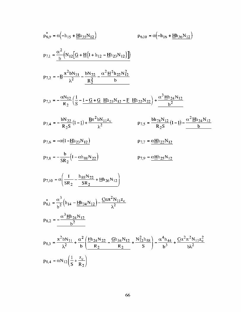
• ( )P6,9 = ct -h15 + Hh35N12 P6,10 = ct(-hl6 + Hh36N12)

Gt2

p_,__-_(N_[_+-{_+h_-"_h_3N_}])

_2bNll bN22 ct2 H2h22N22

P7,2 = -- _2 R2 b

P7,3 = ctN12 {1 )R2 _S -1-G+G Hh23N12-F Hh22N22. +

_3Hh24N12

b 2

B_2bN1 lZcbN22 (1-!)+

P7,4 = R2 S )2bh78N12 (1-1)-

P7,5 -

Gt2Hh24N12

P7,6 = -Ct(1-Hh23N12) P7,7 = _I-Ih22N12

b (1-cth88N22)P7,8 = SR 2

P7,9 = ctHh25N12

{ 1 h88N22 '_

P7,10 = ct_ + Hhz6N12SR 2 SR 2 )

Gt3• C_g2NllZc

P8,1 =_-(h14-Hh34N12) -- _2

ct3Hh24N12

P8,2 = b2

7t2bNll ct 2 {__Fh24N22 G__h34N12

P8,3 - )2 + _ R2 R2

P8,4 = ctN12 +

-I-N22h88 Gt4h44

S b 3

2C_2_2NllZc

+--

b)_2

66

P8,5=ctN12h78 ct3h44 Co:g2NllZc 2

+

S b 2 )v2

ct2h24 b

P8,7 - b R 2

cth88N12

P8,8 - S

ct2h45

P8,9 = b

P8,10 = ---

P9,2 =

or2 {h46 + h88N12b S )

B_2bNllZc

)v2 N12(,_P9,3 - S

bN22(l_ Zc ) ---_t2bNll z2P9,4- S -_2 + )v2P9,5 =

P9,8 b( 1 z_2 ) ( 1 z___ )= - P9,10 =-ct 1+_ S

_2 OI2bNllZc

Pl0,1 =--b-(h14-_Hh34N12) -- _2

Ct2 L-mth24N12

P10,2 = b

PlO,3 -

P10,4 -

_2 ct3h44 C---_g2N1 lZ2cth78N12s + (Fh24N22- Gh34N12 ) b2 I- )v2

bh78N22

S

P10,5 = bh77

2bh28N22 ct2h44 C___2bN1 lZc

+

S b )v2

where

_tb

)v

67

S = 1- h88N22

The expressionsfor the elementsof the T and P matricesfor the caseof classical

platetheoryareobtainedby settingthetransverse-shearstrains,_'13and_'23,equalto zero

1and using the resulting expression_)1= w,1 (recall that equals to zero). The

R1

partially invertedstress-strainrelationsgiven in Eq. (3.11),aremodified such that m12

and K_2are interchanged. For the classical case,only four stability equations,Eqs.

(2.16a), (2.16b), (2.16c), and (2.18a) are used since Eq. (2.18b) is satisfied by

incorporationinto thefinal form of Eq. (2.16c). The samestepsusedfor thetransverse-

shearcasearefollowed to generateT andP matricesof ordereight. The elementsof the

T andP matriceswith a superscript* givenpreviouslyfor thetransverse-shearcasealso

apply for theclassicalcaseif 1 is subtractedfrom any indexgreaterthan4. Thenon-zero

elementsof theT matrix thatarenot givenin theresultsfor transverseshearare

t6,1=_- E H h23N22N12-G H h22N122-E N22- Eh36N22-Gh26N12

t6, 2 = -b- F H h22N22N12-GH h23N22 +G N12-_2 [Fh26N22-Gh36N12])

t8,1 = -_(Eh36N22 - Gh26N12) t8, 2 = -_(Eh26N22 -Gh36N12)

The non-zero elements of the P matrix that are not given in the results for transverse

shear are

h36 )Pl,2 = -ct 1 + -_2 - --Hh23N12P 1,4 = -2cth 36

68

-_(h26 - H__h22N12 )P2,2 = _ R2

P3,4 = b

P4,4 = 2c£h56

P2,4 = -2c£h26

c£( h56 - Lm-Ih25N12P4,2 = _ R2

c£2N12 ( [ h36 ]) c£2h16P5,2- b G+H l+hlz+---H hz3N12R2 -- bR 2

-2c£2 (hi6 - Hh36N12 )P5,4 - b

c£2N12 ( [ h36 ]) c£2h16P6,1- _ G+H l+hlz+--R--7- 2 -H hz3N12 bR2

Gt2 { h66 ) -P6,2 =--_-_-_22 +H__N1212h26_H__h22N12] B_2bN11£2

C£3 (h46 + H__h24N12) + c£N12 (1 + G- GP6,3 = 7_ R2 R2

c£_Fh26N22 c£N12

R 2 R 2

Hh23N12 + F Gh36 ]Hh 22 N 22 + ----_2 ,)

2c£ 2 (h66 + H__h26N12 )P6,4 - b _ R 2bN22 (1-1)+

R2

__B_2bN1 lZc

_2

h36 )P6,5 = -c£ 1 + --R--7-2 - L_-Ih23N12 -_(h26 - Hh22N12)P6,6 = _ R2

bP6,7 = ---

R2 -_(h56 - Hh25N12)P6,8 = _ R2

69

ot 3 C._aI2N 1 lZc

P7,1 = 7(h14 ---Hh34N12)- L2

_3 (h46 +Hh24N12 )P7,2 = - b--T_ R2

P7,3 -_2bNll ct 2 ct4h44

)v2 + bR-----7( --Fh24 N 22 - GNlzh34) b 3

Cct2g2NllZ2+-

b)_2

2ct3h46 ctN12zc ct2h34

P7,4 = ctN12 b2 + P7,5 -R 2 b

ct2h24 b ct2h45

P7,6 - b R 2 P7,8 = b

= _2 [2- zcP8,1 y(hl6 _-_-2 ] - 2L_ 36 N 12.)

P8,2 = --- bR2 [h66 2 Zc - ---g2bNllZc

3h46(zc)( zc)+2 P8,3 = b2 2-R--72 +ctN121-R--72 R--7(Fh26N22-Gh36N12)

20t2h66 (2_ z_-_--2)(z-_-2) B--g2bNllZ2= +bN22 1- +P8,4 b )v2

p,,, p8,6: h26(2_

p8,8: h56(2_

70

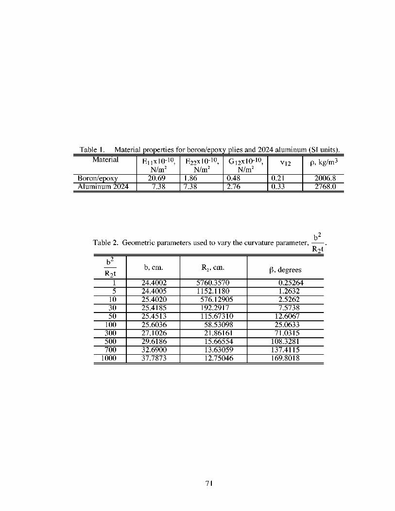
Table 1. Material properties for boron/epoxy plies and 2024 aluminum (SI units)•

Material Ell x 10-1°, E22 x 10-10, G12 x 10-10, v12 p, kg/m 3N/m 2 N/m 2 N/m 2

Boron/epoxy 20.69 1.86 0.48 0.21 2006.8Aluminum 2024 7.38 7.38 2.76 0.33 2768.0

Table 2. Geometric parameters used to vary the curvature parameter, --b 2

R2t

b 2

R2tb, cm. R2, cm. 13, degrees

1 24•4002 5760•3570 0•25264

5 24•4005 1152•1180 1•2632

10 25•4020 576•12905 2•5262

30 25•4185 192•2917 7•5738

50 25•4513 115•67310 12•6067

100 25•6036 58•53098 25•0633

300 27•1026 21•86161 71•0315

500 29•6186 15•66554 108•3281

700 32•6900 13•63059 137•4115

1000 37•7873 12•75046 169•8018

71

©

¢.,J

¢.,J

©

¢.,J

©

¢.,J

,.Q

Z

©

¢.,J

,.Q

©

¢.,J

¢--I¢¢3

Z

_._._._._._._._._._

72

_ Z

o _

©

©

z

73

©

©

Z

Z >-.

Z

©

t'-- _ _ t'--

Z

Z

¢¢3

_._._._._._._._._._

Z

74-

II

,.Q

©

Z

°_

• ©

II _

z _o_

Z _

_ •

___ _ "_

_'_'_'___

"__ Z

75

°,,-_

;>

©

©

..=

,.o

z

©

z _

©

¢¢3

z _ t_

t_

t'--

¢¢3

r',l _'-1

¢¢3

r',l t--

©

©

t"-I

z

©

76

©

©

¢¢3

zZ

¢'3

_',1 ¢'-I

¢_.-

II

oo rOo

_°o r_

=

::::3 _,_

"_ _,._ _ _

_ff ..dN

2

=

=

©

o

oo

©

=©

©

o

©

o° 11

o=

,,,,_ i

_ Z

0 =i =

_Z

Z

©

=i

c¢3i

C¢3i

t--c¢3i

C¢3i

77

_ o

,._'

_-_

_._

_'_'_'_'_'_'_'_

_._._._._.<.<._

II

©

(L) r_ °_

©

_wJ°,._

°,._

°_ _

E-

?S

Figure1.1 Typical longitudinallystiffenedplatestructures.

Figure1.2 Segmentedrepresentationof curved-plate geometry currently used byVICONOPT.

79

_3

_)1

m12 ml 1 m21

_3

............... \\

_1 _2

nl 1 n21 n22n12

Figure 2.1 Curved-plate geometry and sign convention for buckling displacements,rotations, moments, and forces.

80

_3

/// ",,"\

/" \',,.

N 11 N22

\\

\

\_2

_3

["/

//

_2

Figure 2.2 Sign convention for applied in-plane loads and relation of reference surfaceto centroidal surface.

81

tk

Zk

First lamina

b

kth lamina

Referencesurface

Figure 2.3 Curved laminate geometry.

82

Plate 1 Plate 2

*1 U2

W

*1

n

_----D--U2

_2

(a) plates 1 and 2 coplanar

*1 U2

U2 +O)l__

(b) plate 2 rotated to 0=+90 °

*1 U2

*n _w__ _2

+0

,1

(c) plate 2 rotated to arbitray angle, 0

Figure 3.1 Displacements and rotations at a typical plate junction.

83

Nil

p,

p,

p,

i ............

I-

I-

I-

Figure 4.1

E = 10.0x 106 psi

v12 = 0.33

p = 0.1 lb/in. 3

Long isotropic (aluminum) cylinder subjected to uniaxial compression.

84

1100-

1000

900

Nllcr' 800lb/in.

700

600

_k/--- Theoreticalresult(Ref.[48]). m

Curved-plate analysis j

500 I I I I I I I I0 20 40 60 80 100 120 140 160

Number of segments

Figure 4.2 Convergence of VICONOPT segmented-plate results as a function of thenumber of segments used in the approximation.

85

NormalizedCPUtime

Figure4.3

25-

20-

15-

10-

5-

0

Segmented-platetheoryCPUtimesnormalizedwith respectto curved-platetheorytime

- - Segmented-platetheory,SDPTSegmented-platetheory,CPT

J

/

/

/

/

I"

J

J

f

j.

J

j.

J

J

s j

'_'7 ......... i......... i ........ i ......... i ......... i20 40 60 80 100 120 140 160

Number of segments

Normalized CPU time requirements for the segmented-plate approach as afunction of the number of segments used in the approximation.

86

N22

N12

Nll

Figure 4.4 Positive applied in-plane loads on a long, curved plate.

nominal ply

kness004cm_" .............. b ..........._ _._...Boron/epoxy

[0/90/-+45]s

25.4 cm --

Figure 4.5 Symmetrically laminated curved plate with clamped longitudinal edgessubjected to applied in-plane loads.

87

Nil

105

65

4

Nll 3cr,

N/m 2

104

103

1

Figure 4.6

..... Curved-plate theory, physical strains __- - Segmented-plate theory, physical strains _-

---- Curved-plate theory, tensorial strains j_

........ I ........ I ........ I2 3 4 5 67 2 3 4 5 67 2 3 4 567

10 100 1000

Curvature parameter, b2/R2t

Critical value of stress resultant Nil for buckling of a symmetricallylaminated curved plate with clamped longitudinal edges.

88

N22

1049

8

7

6

N22cr, 5

N/m4 ..... Curved-plate theory, physical strains

- - Segmented-plate theory, physical strains- - - Curved-plate theory, tensorial strains

Reference [32]

_n3 ........ I ........ I ........ IJLV 2 3 4 5 67 2 3 4 567 2 3 4 567

1 10 100 1000

Curvature parameter, b2/R2t

Figure4.7 Critical value of stress resultant N22 for buckling of a symmetricallylaminated curved plate with clamped longitudinal edges.

89

N12

1059

8

7

4

N12cr '

N/m 3

104

Figure 4.8

..... Curved-plate theory, physical strains- - Segmented-plate theory, physical strains _"- - - Curved-plate theory, tensorial strains

........ I ........ I ........ I2 3 4 5 67 2 3 4 567 2 3 4 567

1 10 100 1000

Curvature parameter, b2/R2t

Critical value of stress resultant N12 for buckling of a symmetricallylaminated curved plate with clamped longitudinal edges.

90

1049

8

7

N 6cr, 5

N/m4

..... Curved-plate theory, physical strains- - Segmented-plate theory, physical strains- - - Curved-plate theory, tensorial strains

Reference [32]

_-1_13,_, ........ I ........ I ........I

2 3 4 5 67 2 3 4 567 2 3 4 5671 10 100 1000

Curvature parameter, b2/R2t

Figure 4.9 Critical value of stress resultant Nll=N22=N12 for buckling of a symmetricallylaminated curved plate with clamped longitudinal edges.

91

ul andw = 0

on longitudinaledges76.2cm. /

25.4 cm.

Section A-A

+45 ° B/E _ I,,

,,-o D,,_ _-___, 0.014 cm.-a'l'3 D/lff_ _ (typical)

+45 ° B/E

-45 o B/E _" _ _, . _tAmminum " 0.0508 cm.

Figure 4.10 Unsymmetrically laminated aluminum and boron/epoxy (B/E) curvedplate with simply supported edges subjected to applied in-plane loads.

92

N1 lcr '

N/m

250,000 -

200,000 -

150,000 -

100,000 -

50,000 -

..... Curved-plate theory, physical strains- - Segmented-plate theory, physical strains /- - - Curved-plate theory, tensorial strains /"

I I I I I I I0 2 4 6 8 10 12 14

Number of boron/epoxy plies

Figure 4.11 Critical value of stress resultant Nll for buckling of an unsymmetricallylaminated aluminum and boron/epoxy (B/E) curved plate with simplysupported longitudinal edges.

93

N12

140,000-

120,000-

100,000-

N12cr,80,000-N/m

60,000-

40,000 -

20,000-

..... Curved-platetheory,physicalstrains- - - Segmented-platetheory,physicalstrains- - Curved-platetheory,tensorialstrains

Reference[32]

All VICONOPTresults

Reference[32]

I I I I I I I0 2 4 6 8 10 12 14

Numberof boron/epoxyplies

Figure4.12 Critical value of stressresultantN12 for buckling of an unsymmetricallylaminated aluminum and boron/epoxy (B/E) curved plate with simplysupported longitudinal edges.

94

External pressure, p

t=O.1 in.

R2 = 10.0 in.

N22, equivalent

hoop load

ul restrained along longitudinal edges

E = 10.0x 106 psi

3/12-- 0.33

p = 0.1 lb/in 3

N22, equivalent

hoop load

Figure 4.13 Isotropic (aluminum) long cylindrical tube subjected to uniform externalpressure loading.

95

Nil

Simply supported

S ends 2

240 in.

Section A-ASolid wall

I O. 1 in. nom.T

/

' iAluminum

Section A-A

Honeycomb sandwich

0.5 in. nom.

0.1in. nom. l _ l

Aluminum _ /- KorexTM

facesheets honeycomb core

Figure 4.14 Cylindrical shell subjected to uniform axial compression (Nll loading).

96

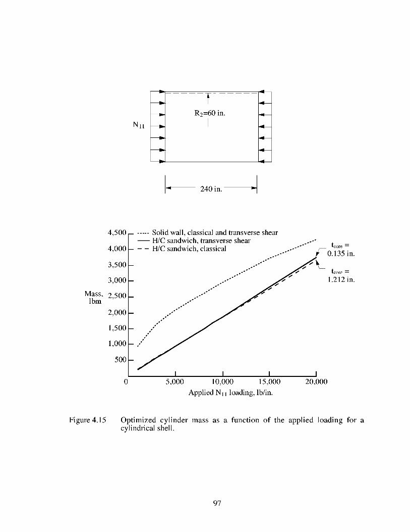
Nil

w__

mllb

mira,.

mlb,

mlb,

Re=60 in.

"' 240 in.

Mass,lbm

4,500

4,000

3,500

3,000

2,500

2,000

1,500

1,000

5OO

...... Solid wall, classical and transverse shear

H/C sandwich, transverse shear ..... ..-- tcore =

- - - H/C sandwich, classical ...... _ 0.135 in.

.-"'" tcore =

- ..-" 1.212 in.

s _

s

s t

s S

I I I I5,000 10,000 15,000 20,000

Applied Nll loading, lb/in.

Figure 4.15 Optimized cylinder mass as a function of the applied loading for acylindrical shell.

97

REPORT DOCUMENTATION PAGE FormApprov_{?M[_ NR, ft7fH-ftlt:lt:l

Public reporting burden for this collection of information is estimated to average 1 hour per response, including the time for reviewing instructions, searching existing datasources, gathering and maintaining the data needed, and completing and reviewing the collection of information. Send comments regarding this burden estimate or any otheraspect of this collection of information, including suggestions for reducing this burden, to Washington Headquarters Services, Directorate for Information Operations andReports, 1215 Jefferson Davis Highway, Suite 1204, Arlington, VA 22202-4302, and to the Office of Management and Budget, Paperwork Reduction Project (0704-0188),

Washington, DO 20,503.1. AGENCY USE ONLY (Leave blank) 2. REPORT DATE 3. REPORT TYPE AND DATES COVERED

August 1999 Technical Memorandum4. TITLE AND SUBTITLE 5. FUNDING NUMBERS

Development of Curved-Plate Elements for the Exact Buckling Analysis ofComposite Plate Assemblies Including Transverse-Shear Effects WU 522-11-41-01

6, AUTHOR(S)

David M. McGowan

7, PERFORMING ORGANIZATION NAME(S) AND ADDRESS(ES)

NASA Langley Research Center

Hampton, VA 23681-2199

9, SPONSORING/MONITORING AGENCY NAME(S) AND ADDRESS(ES)

National Aeronautics and Space Administration

Washington, DC 20546-0001

8. PERFORMING ORGANIZATIONREPORT NUMBER

L-17882

10, SPONSORING/MONITORINGAGENCY REPORT NUMBER

NASA/TM- 1999-209512

11.SUPPLEMENTARYNOTESThe work in this report was submitted to the faculty of Old Dominion University in partial fulfillment of the

requirements for the degree of Master of Science, Engineering Mechanics, in May 1997.

12a, DISTRIBUTION/AVAILABILITY STATEMENT

Unclassified-Unlimited

Subject Category 39 Distribution: Nonstandard

Availability: NASA CASI (301) 621-0390

12b, DISTRIBUTION CODE

13. ABSTRACT (Maximum 200 words)

The analytical formulation of curved-plate non-linear equilibrium equations including transverse-shear-deformation effects is presented. A unified set of non-linear strains that contains terms from both physical and

tensorial strain measures is used. Linearized, perturbed equilibrium equations (stability equations) that describethe response of the plate just after buckling occurs are derived. These equations are then modified to allow the

plate reference surface to be located a distance zc from the centroidal surface. The implementation of the newtheory into the VICONOPT exact buckling and vibration analysis and optimum design computer program is

described. The terms of the plate stiffness matrix using both classical plate theory (CPT) and first-order shear-deformation plate theory (SDPT) are presented. The effects of in-plane transverse and in-plane shear loads are

included in the in-plane stability equations. Numerical results for several example problems with differentloading states are presented. Comparisons of analyses using both physical and tensorial strain measures as well

as CPT and SDPT are made. The computational effort required by the new analysis is compared to that of theanalysis currently in the VICONOPT program. The effects of including terms related to in-plane transverse and

in-plane shear loadings in the in-plane stability equations are also examined.

14. SUBJECT TERMS

Curved plates, buckling, transverse shear deformation, composites,

optimization, finite strips

17. SECURITY CLASSIFICATION 18. SECURITY CLASSIFICATION 19. SECURITY CLASSIFICATIONOF REPORT OF THIS PAGE OF ABSTRACT

Unclassified Unclassified Unclassified

NSN 7540-01-280-5500

15. NUMBER OF PAGES

11216. PRICE CODE

A0620, LIMITATION

OF ABSTRACT

UL

Standard Form 298 (Rev. 2-89)Prescribed by ANSI Std. Z-39-18298-102