Development of Constancy Control and Calibration Protocols for

Master Thesis RF9300, 30 HP

VT 08

Development of Constancy Control and Calibration Protocols for Radiation Monitor

Devices and Estimations of Surface Dose Rates from Radioactive Waste Containers Used at

University of Gothenburg.

Dan Thorelli

Supervisors:

Mats Isaksson and Annhild Larsson

Department of Radiation Physics

University of Gothenburg 2008

Abstract

Radiation monitor detectors are the most important tool available for evaluating and examining the workplace. It is important to only use the detector for measurements in situations it is designed for and to have an accurate calibration.

The regulation SSI FS 2000:7 [12] states, in 9 § regarding quality assurance, that a quality handbook should be available. In dealing with extensive laboratory work, defined in 2 §, the handbook should contain routines for calibration and constancy control of radiation monitoring devices. This thesis deals with a development of a simple constancy control routine. As a result a correctly calibrated radiation monitor that measures or should not give a reading that is lower than E. E is calculated

for a few sources of interest.

The maximum amount of radioactivity allowed to be disposed of, depending on the nuclide, and the maximum surface dose rate allowed for waste containers is given by the regulations in SSI FS 1983:7 [13]. This thesis deals with a few estimations of surface dose rates from waste containers filled with gamma or beta emitting nuclides.

The investigated instruments that measure the ambient dose equivalent could not be said to give a reading that is lower than the calculated effective dose, taking statistical factors in mind. This is an important result as it means that they will not underestimate the effective dose that is related to the risk of the exposure.

Unfortunately none of the used sources are an ideal constancy control source. A more appropriate constancy and control source could be a Cs-137 source with an activity of 4 MBq. The effective dose from the new source could be calculated, and the instruments could be re-measured with the new source by following the general measurement steps.

2

Introduction 1

Working with radionuclides 1

Radiation protection 3

Units and concepts 4

Disposal of radionuclides 6

Microshield 7

Radiation Detectors 7

Detector efficiency 12

Energy response 14

Calibration of radiation monitoring instruments 14

Material and methods 16

Point dose estimations method 16

Volume source estimations method 18

General measurement steps 22

Constancy control and calibration method 23

Results 26

Dose levels around waste containers 26

Calibration and constancy control 29

Discussion 32

References 38

Appendix

Nuclides used at Gothenburg University

Volume source definitions in Microshield

Investigated detectors with spread sheet results

1

1. Introduction

When ionizing radiation is used in laboratory work, or other purposes, it is important to make sure that the workplace is safe and to minimize the risk to the worker, as in any other field of work. Radiation monitor detectors are the most important tool available for evaluating and examining the workplace. A single type of detector that could measure all form of radiation with the same accuracy would be convenient, however no such radiation detector exists. Instead a number of detectors, all with different properties, are used to measure the radiation from different forms, at different intensities and from different nuclides. This makes it important to only use the detector for measurements in situations it is designed for and to have an accurate calibration. The regulation SSI FS 2000:7 [12] states, in 9 § regarding quality assurance, that a quality handbook should be available. In dealing with extensive laboratory work, defined in 2 §, the handbook should contain routines for calibration and constancy control of radiation monitoring devices. This thesis deals, in part, with development of a simple constancy control and calibration method for radiation monitoring devices, with the main focus set on a simple constancy control. The method needs to be simple not to be skipped or ignored.

At laboratories or institutions that deal with radioactivity, there will eventually be a need for disposal of some radioactivity. If the disposal is solid waste and packaged in a container, a measurement of the surface dose rate needs to be done. The measurement is made to make sure the dose rate is below the legal limit, before the container is sent away. The maximum amount of radioactivity allowed to be disposed of, depending on the nuclide, and the maximum surface dose rate allowed is given by the regulations in SSI FS 1983:7 [13]. This thesis deals with a few estimations of surface dose rates from waste containers filled with gamma or beta emitting nuclides.

2. Working with radiation

2.1 Radiation

An unstable nucleus can, in every moment, decay by emission of radiation with a certain probability. The emitted radiation is nuclide specific, and can be gamma, beta or alpha radiation. The probability for decay cannot be influenced in any physical or chemical form. The decay modes of interest, in this thesis, are gamma and beta decay. Alpha radiation will not be considered due to the measurement setup requirements to get a satisfactory measurement.

2.1.1 Gamma radiation (γ)

Photons travelling in a material, with energies of interest in laboratory work, are subject to an interaction by either photoelectric absorption, compton scattering or pair production. The sum of the probability for each interaction is included in the linear attenuation coefficient, µ.

2

If a shied is placed between an emission point and a measuring point , the number of transmitted photons (N) relative to incoming number of photons ( ) without the shield, is given by equation (1)

(1)[1]

Where µ is the linear attenuation coefficient, x is the thickness of the material, N is the number of transmitted photons and is the number of incoming photons.

Equation (1) show that the photons are subject to an exponential attenuation. Thus a fully absorbing shield cannot be constructed. The shield has to be designed to reduce the photon fluence to an acceptable level instead. When half of the number of incoming photons has interacted in the material, a useful expression in radiation protection can be derived. Equation (2) gives the half value layer (HVL).

(2)[2]

Where µ is the linear attenuation coefficient

This is the thickness of a material that will reduce the photon fluence by half of its original value, and is a useful guide when deciding shield dimensions.

2.1.2 Beta radiation (β)

There are two types of beta decay;

- , electron decay - , positron decay

decay occurs in nuclides with an abundance of neutrons and decay occurs in nuclides with an abundance of protons. The beta particle share the energy released (in a decay) with a neutrino, that is created alongside the particle. The energy distribution between the particles is governed by statistics. There are two energies of interest for the beta particle;

• The maximum beta energy

A beta particle emanating with maximum energy occurs when it receives all of the energy released in a decay. The maximum energy can be used to calculate the particles maximum range. When the range is known it can be used to construct appropriate shielding. If the dimensions of the shield exceed the maximum range of the beta particle, in the material, no beta particles will emanate from the surface of the shield. Equation (3) can be used to estimate the range for beta particles with maximum energy between 0.01 to 2.5 MeV.

(3)[3]

Where R is the range in mg/ and E is the maximum beta energy in MeV

3

When the beta particle interacts in the shield there is a chance for a bremsstrahung photon to be produced. The probability, P, for the emission can be approximated by the expression;

(4)[1]

Where Z is the atomic number of the material and m is the mass of the particle.

Equation (4) show that the probability for emission increases with decreasing particle mass. This makes the probability for emission higher for beta particles, compared with other more massive charged particles. Equation (4) also shows that a shield should be constructed in materials with low atomic numbers, to decrease the probability for photon contribution.

• The mean beta energy

The mean beta energy is approximately a third of the maximum beta energy [11]. The mean beta energy is used in dose calculations.

2.2 Radiation protection

The recommendations made by the ICRP (International Commission on Radiation Protection) have a profound influence on radiation protection all over the world. One important presumption made by the ICRP, is that even small radiation doses can cause harmful effects. The three main principles of radiation protection are;

• Justification To prohibit practices involving additional exposures unless they produce sufficient societal benefits. The benefits should be weighed against the risks.

• Optimization The optimization principle requires the radiation exposure, to the worker, to be as low as reasonably achievable, or ALARA. Implementing ALARA in practice involves;

- Reducing the source A way of eliminating the radiation source can be done by using ultrasound instead of diagnostic x-ray wherever possible. Source reduction is also a reduction of the dose rate, and can be done in several ways. One way is to properly ventilate areas where airborne radioactivity is present.

- Source containment To make sure that proper containment, ventilation and filtration is used.

- Time The minimization of the time that radioactive materials are handled, less time leads to a lower dose. This can be achieved by practice the procedures without activity present. The work should be performed quickly, but without rushing.

- Distance

4

Maximization of the distance from the source. For a gamma point source, the dose is inversely proportional to the square of the distance. A significant dose reduction can be achieved with increased distance, for example by using distance tools

- Shielding Shielding should be used wherever it is necessary to reduce or eliminate the radiation exposure to the worker. By placing a shield between the source and the worker, the exposure can be reduced to an acceptable level. The type and thickness of the material needed to reduce the dose to a safe level varies with the type and amount of the nuclide.

• Dose limits Limits of radiation exposure to individuals. SSI issues regulations regarding dose limits in Sweden, where the most important are

- SSI FS 1998:4

States that the dose limit for workers, and public, exposed to ionizing radiation from the workplace is 50 mSv per year and a maximum of 100 mSv for five consecutive years. The dose limits does not apply for patients subject to medical radiation treatments, people helping patients during medical radiation treatments (of their free will), voluntary test-subjects and in emergency rescue situations.

- SSI FS 1998:3

Regulations for categorizing the worker in two categories, A or B. If the risk is not insignificant on an annular basis for: the effective dose to exceed 6 mSv, the equivalent dose to one eye lens exceeding 45 mSv or the equivalent dose to the hands, forearm or skin exceeding 150 mSv the worker should be placed in category A. The effects of accidents that can lead to high exposures that could justify the placement in category A has also been taken into mind. Workers that are not placed into category A are placed into category B

- SSI FS 1998:6

States that a worker classified as category A should be subject to regular medical examinations and wear a radiation dosimeter. If the result from the medical examinations is not satisfactory the worker can be limited or forbidden to work with radiation as a category A worker.

2.3 Units and concepts

2.3.1 Units

5

The absorbed dose (D) is a measure of the energy absorbed per unit mass from ionizing radiation in a medium. Different types of radiation can cause different amount of damage. The absorbed dose does not take that into account. To calculate the total biological effective dose for different types of radiation, the differences must be considered.

The equivalent dose (H) is given when the absorbed dose is multiplied by a weighting factor that reflects the radiations ability to cause damage, equation (5). The weighting factor is dependent on the ionization density, for gamma radiation the factor is set to unity, and other types of radiation are related to the value according to their ionization densities.

(5)[4]

Where is the weighting factor for the radiation type and is the absorbed dose in the organ of radiation type .

All organs and tissues do not have the same sensitivity when exposed to the radiation. And in most cases the body is not uniformly irradiated. The effective dose (E) takes this into account and is given as the equivalent dose multiplied by a organ weighting factor, equation (6)

(6)[3]

Where is the weighting factor for different types of organs.

One of the main advantages of using the effective dose is that the risk of a radiation exposure to one specific organ can be compared with the risk of a whole body exposure.

Ambient dose equivalent, [Sv]

The ambient dose equivalent is the dose equivalent in a point in a radiation field that corresponds to the dose in an expanded and parallel radiation field (see figure (1)) at the depth of 10 mm in the ICRU sphere [5]. Instruments that measure the ambient dose equivalent should be directional independent.

Figure (1). An expanded and parallel radiation field

Personal dose equivalent, [Sv]

6

is the dose at a depth d under the placement point of the meter. The readout

from the meter should be directional dependent. The depths most commonly used are 0.07 mm and 10 mm, to simulate skin or organ exposure.

Relationships between units in radiation protection

Figure (2) show the quotient between the effective dose, (E), and the ambient dose equivalent, ( ), for photon radiation in different geometries.

Figure (2). The quotient between E and plotted versus photon energy for several different geometries. [5]. AP: Parallel radiation field, directed as figure (1); ISO: Isotropic radiation field.

Figure (2) show that is larger than E in many different geometries. Similarly it has been shown that is larger than E in most geometries [5]. As a result a correctly

calibrated radiation monitor that measures or should not give a reading that is

lower than E.

2.3.2 Concepts

-

ALI stands for Annual Limit on Intake, and is defined, in ICRP 30 [14], as the annual intake of a nuclide that would lead to an effective committed dose equivalent below or equal to 50 mSv and an annual dose equivalent to any organ or tissue below or equal to 500 mSv. The definition can be expressed as equation (7) and equation (8)

Sv (7)

Where is the tissue weighting factor and is the total committed dose equivalent in tissue T

Sv, for all T (8)

Where is the total committed dose equivalent in tissue T

7

Different values exist for inhalation and ingestion, is the lowest of these values for the nuclide of interest.

- DAC

The ALI value only gives an intake limit for a specific nuclide. No considerations of the intake rate or the atmospheric/environmental concentrations that leads to the intake limit are made. For airborne contaminations of radioactivity the Derived Air Concentration (DAC) takes these effects in mind. The DAC, for any radionuclide, is that concentration in air (Bq/ ) which, if worked for a year, would result in the ALI value for inhalation. The DAC can be calculated according to equation (9)

(9)[3]

Where ALI is the intake limit for the nuclide [13] and 2400 is the volume of air a standard person will inhale during a year at work.

- Radiotoxicity

For laboratory work with unsealed substances, the regulation SSI FS 2000:7 classifies nuclides into four categories dependent on their radio toxicity (A to D). Where class A is highly toxic and class D is the least toxic. The amount of activity that is allowed to handle during extensive laboratory work is given in [13]

2.4 Disposal of radionuclides

A certain amount of radioactive waste can be disposed of at the local landfill or in the sewer. The amount depends on the radioactive nuclide, and is defined by the nuclides value. This is regulated by SSI FS 1983:7 [13]. The limitation does not apply to waste from patients subject to treatment or diagnostics with radioactive substances.

2.4.1 Regulations for solid waste

The maximum amount of activity, per month, allowed to be disposed of at the local landfill is 10 .

The maximum amount of activity placed in one waste container should not exceed 1 , and the maximum surface dose rate should not exceed 5 µGy/h. The waste containers should not contain any sealed source with an activity above 50 kBq.

2.4.2 Regulation for liquid waste

The maximum amount of activity that can be disposed of in the sewer, per month, is 10 ALImin. The maximum activity per disposal should not exceed 1 or 100 MBq. After each disposal significant amount of water should be used to flush the system.

8

2.5 Microshield

Microshield is a radiation shielding and dose assessment program for gamma emitting nuclides. Microshield is written by Grove Software Inc, situated in the USA. The version used in this thesis is 6.20.

Microshield is used to estimate the value of the effective dose for the gamma emitting calibration and constancy control sources at the measurement points. Microshield is also used to estimate the surface dose rate from the waste containers filled with gamma emitting nuclides.

3 Radiation detectors

The human body lacks a sense for detecting radiation. Instead the detection is based on physical and chemical effects produced by radiation in the exposed material, other than man. Common effects produced by the radiation are ionization in gas, ionization and excitation in solids, chemical changes and neutron activation. A detector is usually constructed with one of these effects in mind.

3.1 Gas detectors

When the gas is exposed to ionizing radiation it produces ionization and excitation effects in the detector gas. This is the principle on which the gas filled detectors are based. If the detector is exposed to steady state irradiation, the created ion-pairs will be kept constant. Commonly used gas-filled radiation detectors, like ion chambers, proportional counters and GM-tubes, then makes use of the direct ionization created by the radiation.

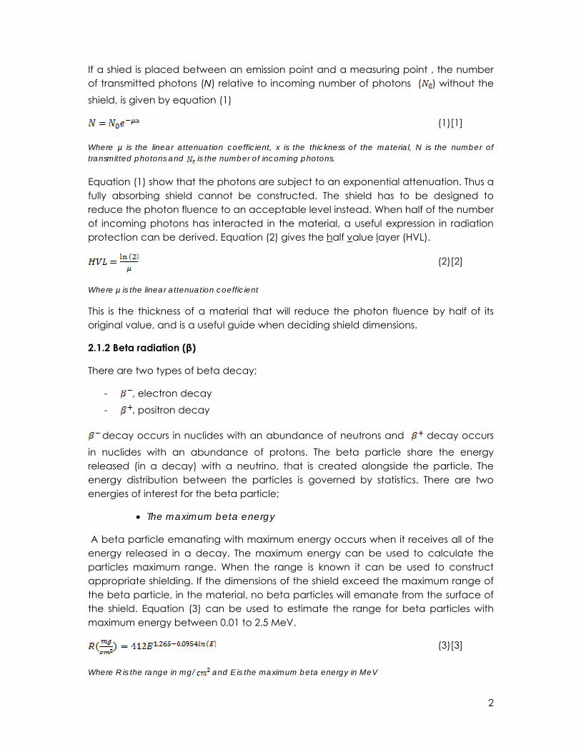
To be able to collect the ion pairs, an electric field is used. When the electric field is present, the electrostatic force start to move the particles (electrons and ions) away from the point of creation. With the applied electric field the moving particles creates an electric circuit, and a current can be measured. Without the electric field the net current is zero. The created ions can be lost due to either recombination or diffusion out of the volume. With increasing electric field, less of the original charge is lost to recombination effects. At a certain level the electric field is strong enough to reduce the recombination to a minimal level and all of the created charge is measured. Further increasing the strength of the electric field, up to a certain strength, has no effect. This is due to the constant formation the ion pairs and an efficient collection of the charge created. This plateau is called ion-saturation and is the area where ion chambers are operated. See figure (3).

9

Figure (3). The pulse amplitude plotted versus the applied voltage of the electric field for two different energies. [6]

One important application for the ion chambers is to measure the absorbed dose in different materials. The absorbed dose can be measured using the Bragg-Gray principle that states that the absorbed dose in a material can be given from the ionization that is produced in a small gas filled cavity, the ion chamber, in the material. Several conditions need to be met for the principle to hold. One important condition is that the cavity, ion chamber, needs to be small compared with the primary and secondary range of the radiation, to minimize the effect it poses on the particle flux.

If the detector gas is air and the detector walls are air equivalent, the chamber can be used to measure the absorbed dose in air. A measurement of the absorbed dose in air is equivalent with a measurement of the gamma ray exposure, which is another important application of ion chambers.

If the electric field is further increased, it will cause an effect called gas multiplication. In the ion saturation region, the electrons and ions simply drift to their collecting electrodes. On their way the particles frequently collide with neutral gas molecules. The ions gain little average energy between the collisions due to their low mobility. The electrons can easily be accelerated in the electric field, due to their low mass, and have high kinetic energy when colliding with a neutral gas molecule. If this energy is high enough to cause ionization in the neutral gas molecule, a second ion pair can be formed. A threshold exists when this second ionization event can take place, due to electrons gain increased kinetic energy with increased electric field. The second electron created in the collision is accelerated in the electric field and can also create new ion pairs; this process is called a Townsend avalanche. The

10

avalanche will terminate when all electrons are collected at the electrode. Using the effects of the Townsend avalanche, given the right circumstances, the secondary ionizations can be kept proportional to the primary ionization events, but the total numbers if ionizations can be increased significantly. This is the region called the proportional region where the proportional counters are used, see figure (3).

Proportional counters are more sensitive to impurities in the detector gas than ionization chambers, which can cause problems due to the formation of many excited molecules or atom states created during the avalanche. The excited molecules decay by photon emission which can cause new ionizations by either photoelectric interaction in the gas or releasing electrons when interacting in the detector wall. In a proportional counter these effects will cause a loss of proportionality, increased dead time and reduced spatial resolution for positioning sensing detectors. By adding another gas, a fill gas, the effects can be reduced by absorbing the photons in a way that does not cause new ionizations. The amplified charge gained when using a proportional counter requires less external amplification of the signal, which makes the proportional counter have an increased SNR (signal to noise ratio) compared with an ion chamber.

Further increasing the electric field will generate a linear amplified response from the detector in a certain region; this is the region of true proportionality. Increasing the electric field beyond this region will cause a non-linear response. The most important contribution to this effect is caused by the slowly moving positive ions. During the time it takes to collect the electrons the ions has hardly moved at all. The slowly drifting ions creates a cloud of positive charge in the detector, if the numbers of ions is high enough they can alter the shape of the electric field. This will cause nonlinear effects to occur; due to the gas multiplication dependence of the strength of the electric field. This region is called limited proportional region and is not a desirable region of operation for any detector. See figure (3).

If the electric field is increased above the limited proportional region, the space charge created by positive ions will determine the output pulse from the detector. The high electric field is used to intensify the avalanches. In ideal conditions one avalanche can trigger another avalanche at another point in the detector. This chain reaction leads to an exponential growth of avalanches in the detector, called a Geiger discharge. The avalanche will continue to a point where the space charge from the ions reduces the electric field below the limit for continued gas multiplication, thus making the process self limiting. The same number of positive ions will be formed to cause the electric field to drop below the threshold of gas multiplication, independent of the number of primary ionization events in the detector. The output pulse from the detector will then be of the same magnitude and all properties of the radiation are lost. This makes the detector only function as a counter. This is the GM-region, see figure (3).

In the GM tube the effects of the excited molecules and atoms, that caused problems for proportional counters, are desirable. The propagation of the Geiger

11

discharge is made possible by the photon emissions. In proportional counters each avalanche is formed in a position that corresponds with the original position of the ionization event. In the GM tube the discharge grows due to random formations of avalanches, caused by the emissions and interactions of the emitted photons by to cover the entire collection wire. This produces a massive amount of positive ions that need to be collected which leads to a high dead time in GM tubes, see figure (4). The increase in signal strength leads to less requirements of external amplification.

Figure (4). The propagation of a Geiger discharge [6]

Special precautions must be taken in Geiger counters to avoid creating a continuous output loop of pulses. When the positive ions arrive at the collecting electrode they are neutralized when combining with electrons from the electrode; in this process energy is released. If this energy exceeds the energy needed to extract an electron from the electrode surface, it is possible that a new free electron can be released and create another Geiger discharge. This effect would then produce a continuous output of pulses from the GM tube. To avoid this effect either external or internal quenching can be used.

Internal quenching is done by adding an additional gas, quench gas, to the detector gas. The quench gas prevents the continuous output by using the effect of change transfer collisions. The quench gas has a lower ionization potential and more complex molecular structure than the detector gas. When the positive ions collide with the quench gas and transfer the charge, the ions are neutralized and the quench gas molecules start to drift to the collection electrode instead. If the concentration of the quench gas is sufficiently high all of the positive ions arriving at the collection electrode will be of the quench gas. When they are neutralized the energy released may go to dislocating the more complex molecular structure instead of releasing an electron from the surface.

External quenching can be done by reducing the high voltage for a specific time after each pulse, below the value for the gas multiplication to take effect.

12

For almost any detector system there will be a minimum amount of time needed for two separate events in the detector to be recorded as two separate pulses. In some detectors the limits are set due to processes intrinsic to the detector itself, in others the surrounding electronic sets the limit. The minimum time needed to separate the two events is called dead time. There is always a probability that true events may be lost due to the randomness of radiation, dead time losses. At high counting rates these losses can become severe, and methods for compensation have to be used to get any accuracy in the measurement. These dead time losses affect almost any detector system, but especially the GM-tube due to its design. The methods of dead time compensation depend on the behavior of the detector system. There are two common models used, a paralyzable or nonparalyzable detector system. The nonparalyzable detector system can give a reading in high intensity radiation fields, the paraplyzable detector system can fail to give a reading at all. The models represent two extreme behaviors of an idealized detector system, where one, or the other, usually describes the true detector system adequately. The two models differ greatly from each other at high dead time losses but predict the same amount of losses at low levels. Measurements taken under conditions with high dead time losses should be avoided, to avoid the increasing error in the correction. When the dead time losses are at 30 to 40 % the uncertainty is high, and efforts should be made to reduce the dead time losses [6]. This can be done by either changing the measuring conditions or by changing the detector system.

3.2 Scintillation detectors

Scintillation detectors are based on the principle of induced luminescence that is produced from the detector material when exposed to ionizing radiation. In scintillation detectors composed of organic materials the molecules are excited through the kinetic energy absorbed from electrons that are released from photon interactions in the detector material. The excited molecules, in the detector, return to their original state by photon emission, and these photons are then collected. In scintillation detectors of inorganic materials the atoms are arranged in a crystal structure, and the crystal is excited by the energy absorbed in the passage of electrons.

The requirements for a good scintillation material are:

• High probability for interaction with photons. • Proportionality between the light emitted and the energy deposited in the

detector • Efficient conversion from kinetic energy to emitted light. • Transparency for the light emitted in the material. • The decay time for the induced luminescence should be short. • A refraction index close to that of glass. • Good optical quality and be able to manufacture in practical detector sizes.

13

The detector material should also be able to respond quickly to radiation. Before the next photon strikes the detector all light from the previous interaction should have been converted. This is essential to get a correct measurement.

The light emitted from the material then strikes the surface of a photo multiplier tube (PM-tube). The front part of the PM-tube, facing the scintillation material, is coated with a light sensitive material. When the photons, produced in the detector material, strike the surface electrons are released. The electrons are then accelerated through the PM-tube by an electric field. During the acceleration the electrons collide with plates, called dynodes, where each collision releases additional electrons. As a result an amplified signal is produced that can be further processed and amplified.

3.2.1 NaI(Tl) scintillation detectors

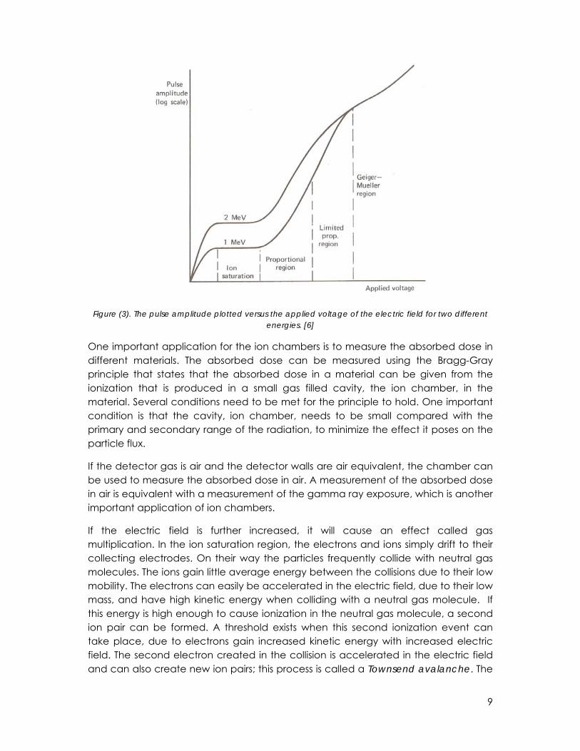
The NaI(Tl) scintillation detector is used for detection of photon radiation. The detector has a relatively good energy resolution, which makes it possible to distinguish between photons with different energies. The photoelectric effect is the dominating way of interaction for low energy gamma rays and the probability for interaction can be approximated by the expression

(10)[1]

Where z is the atomic number of the absorption material and hf is the photon energy.

Iodine has a high atomic number, this makes interaction by photoelectric absorption significant and gives a high probability that the total photon energy gets stored in the detector. With decreasing energy the probability for interaction also increases. This inherent property makes the NaI(Tl) scintillation detector useful in situations where the GM-tube will fail to give a reading. To increase the probability that the emitted photons lies in the visible spectrum, a small amount of thallium is added to the detector. NaI is sensitive to moisture, thus an enclosure of metal is often used. The added metal will attenuate some of the incoming radiation, and reduce the detection efficiency.

3.2.2 Liquid scintillation detectors

The scintillation material in a liquid scintillation detector is composed of a liquid and the sample is mixed with the scintillation liquid. The light emitted from the solution is then registered by a PM-tube in the same way as the other scintillation detectors. The main advantage with a liquid scintillation detector is that samples containing low energy beta and alpha particles can be measured. can be measured with an

efficiency of about 50% [7].

Mixing the sample with the scintillation liquid can be complicated, not all samples can be mixed directly without preparations. Sample containing more than one beta emitting nuclide, with similar energies, can cause problems in distinguishing between the different nuclides. This can be solved with separation methods.

14

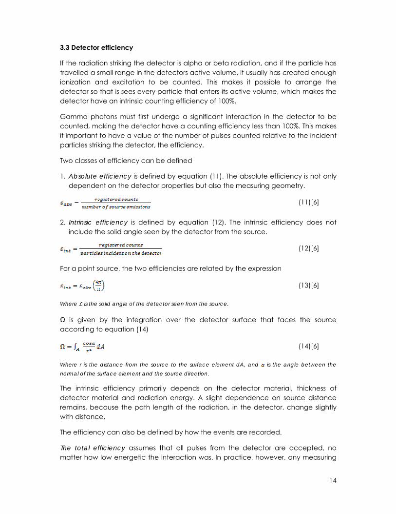
3.3 Detector efficiency

If the radiation striking the detector is alpha or beta radiation, and if the particle has travelled a small range in the detectors active volume, it usually has created enough ionization and excitation to be counted. This makes it possible to arrange the detector so that is sees every particle that enters its active volume, which makes the detector have an intrinsic counting efficiency of 100%.

Gamma photons must first undergo a significant interaction in the detector to be counted, making the detector have a counting efficiency less than 100%. This makes it important to have a value of the number of pulses counted relative to the incident particles striking the detector, the efficiency.

Two classes of efficiency can be defined

1. Absolute efficiency is defined by equation (11). The absolute efficiency is not only dependent on the detector properties but also the measuring geometry.

(11)[6]

2. Intrinsic efficiency is defined by equation (12). The intrinsic efficiency does not include the solid angle seen by the detector from the source.

(12)[6]

For a point source, the two efficiencies are related by the expression

(13)[6]

Where is the solid angle of the detector seen from the source.

Ω is given by the integration over the detector surface that faces the source according to equation (14)

(14)[6]

Where r is the distance from the source to the surface element dA, and is the angle between the normal of the surface element and the source direction.

The intrinsic efficiency primarily depends on the detector material, thickness of detector material and radiation energy. A slight dependence on source distance remains, because the path length of the radiation, in the detector, change slightly with distance.

The efficiency can also be defined by how the events are recorded.

The total efficiency assumes that all pulses from the detector are accepted, no matter how low energetic the interaction was. In practice, however, any measuring

15

system requires the pulse to be higher than a certain pulse-height set to discriminate against electronic noise.

The peak efficiency assumes that only full energy interactions in the detector are counted. These full energy interactions are usually seen as the peak at the end of a differential pulse height distribution.

The quotient, r, of the efficiencies are related by equation (15)

(15)[6]

The peak efficiencies are commonly tabulated, because the full energy events are not as sensitive to scattered radiation and false pulses. The detector should be specified according to both efficiency criteria. The most common efficiency tabulated for a gamma ray detector is the intrinsic peak efficiency. If the detector has a known efficiency it can be used to measure the activity of a radioactive source, equation (16).

(16)[6]

Where S is the number of emitted particles from the source during the measuring time and N is the number of recorded events.

Equation (16) can be rewritten by using equation (13) and using that the source strength (point source) equals the activity multiplied by the sum of the branching ratio ( . The result is seen in equation (17)

A = (17)

Where A is the activity, N is the number of recorded events, is the efficiency and fi is the probability for decay for each emission.

Equation (17) is used for calibration or constancy control purposes for calculating the activity. By solving equation (17) for the efficiency is given, equation (18)

= (18)

Where A is the activity, N is the number of recorded events, is the efficiency and is the probability for decay for each emission.

3.4 Regions of measurement and Energy response

Ion chamber detectors can be used to measure gamma and x-ray radiation down to a few tenths of a mSv/h [8]. At lower levels the chamber dimensions needs to be increased, for incased sensitivity. Although the increase would make the chamber

16

too large for portable use, there is however other designs of ion chambers, like the pressurized ion chamber and liquid ion chamber that can be used at lower radiation levels where the normal ion chamber will fail to give a reading. To measure the radiation in the lower regions a GM-tube or scintillation detector can also be used.

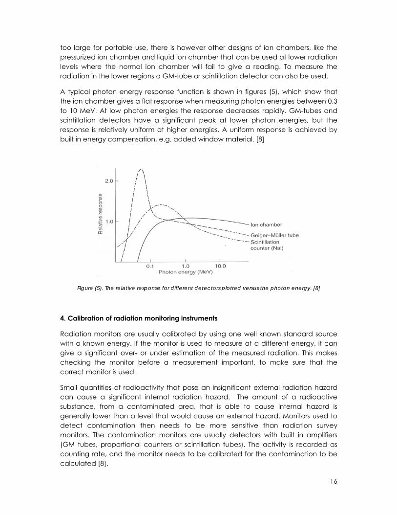
A typical photon energy response function is shown in figures (5), which show that the ion chamber gives a flat response when measuring photon energies between 0.3 to 10 MeV. At low photon energies the response decreases rapidly. GM-tubes and scintillation detectors have a significant peak at lower photon energies, but the response is relatively uniform at higher energies. A uniform response is achieved by built in energy compensation, e.g. added window material. [8]

Figure (5). The relative response for different detectors plotted versus the photon energy. [8]

4. Calibration of radiation monitoring instruments

Radiation monitors are usually calibrated by using one well known standard source with a known energy. If the monitor is used to measure at a different energy, it can give a significant over- or under estimation of the measured radiation. This makes checking the monitor before a measurement important, to make sure that the correct monitor is used.

Small quantities of radioactivity that pose an insignificant external radiation hazard can cause a significant internal radiation hazard. The amount of a radioactive substance, from a contaminated area, that is able to cause internal hazard is generally lower than a level that would cause an external hazard. Monitors used to detect contamination then needs to be more sensitive than radiation survey monitors. The contamination monitors are usually detectors with built in amplifiers (GM tubes, proportional counters or scintillation tubes). The activity is recorded as counting rate, and the monitor needs to be calibrated for the contamination to be calculated [8].

17

Radiation survey monitors are usually calibrated to measure the ambient dose equivalent ( ). This makes it easy to check that the limit of radiation exposure is not exceeded when the energy or direction of the radiation is unknown [5].

There are two methods commonly used when calibrating radiation monitor instruments.

• Indirect calibration (intercalibration) In this method the response from the radiation monitoring instrument under calibration is compared to the response of a reference instrument, see figure (6). The reference instrument used has to be calibrated against a higher quality reference instrument [9]. Care should be taken to minimize the scattered radiation, it can cause problems when detectors have different energy response [8].

Figure (6). Intercalibration [9]

• Direct calibration The radiation monitor that is to be calibrated is placed in a known radiation field from known standard sources. A schematic setup is presented in figure (7). This is the method proposed in this thesis.

Figure (7). Direct calibration [9]

There are several important parameters intrinsic to the radiation monitor that has to be known. The most important that should be thoroughly examined are, sensitivity to radiation, energy response, rate response and temperature response. This is normally done by the manufacturer before the monitor is released to the costumer [8]. A calibration of radiation monitors in the true meaning of the word is beyond this thesis, but the calibration can be investigated, see section 2.

18

The radiation monitors sensitivity is the parameter that most likely will change over time [8]. This makes it the most important parameter to check when performing a constancy control. This can be done by measuring the same source in the same way and recording the results. If the measured value deviates significantly from the expected decrease due to natural decay further investigations could be made.

The reasons for a changed response are various, here are a few examples.

- Power problems. Battery problems or damaged wires

- Electric field problems The collecting electrodes could have been bent or damaged. This would alter the electric field.

- Contamination problems The detector gas could have been contaminated with air from a small leak. Air (oxygen) is an electronegative gas, and could cause problems for many detectors if the concentration is high enough. [6]

When the detector has been repaired it should be recalibrated before being put to use.

5. Material and methods

5.1 Dose rate estimations from point sources

5.1.1 Estimation of beta point dose rates for calibration and constancy control sources

Estimation of the beta point dose rate in air is done to get the conversion factor from cps to dose rate in air (section 5.4). The beta particles strong dependence of air attenuation on energy makes it hard to find a simple expression for the dose rate. No programs like Microshield for beta point source were available. The calculations will only give an approximate value, for methods with higher accuracy see the discussion section for references.

• Estimation by using energy fluence with beta attenuation coefficient

The energy fluence at a distance d from a beta point source can be used to calculate the dose rate at a point in air, and the energy fluence is given by equation (19)

(19)[3][10]

Where r is the distance from the source to the measurement point, is the mean beta energy (in MeV) per decay, is the beta energy attenuation coefficient and is the areal density

The areal density is given by equation (20)

19

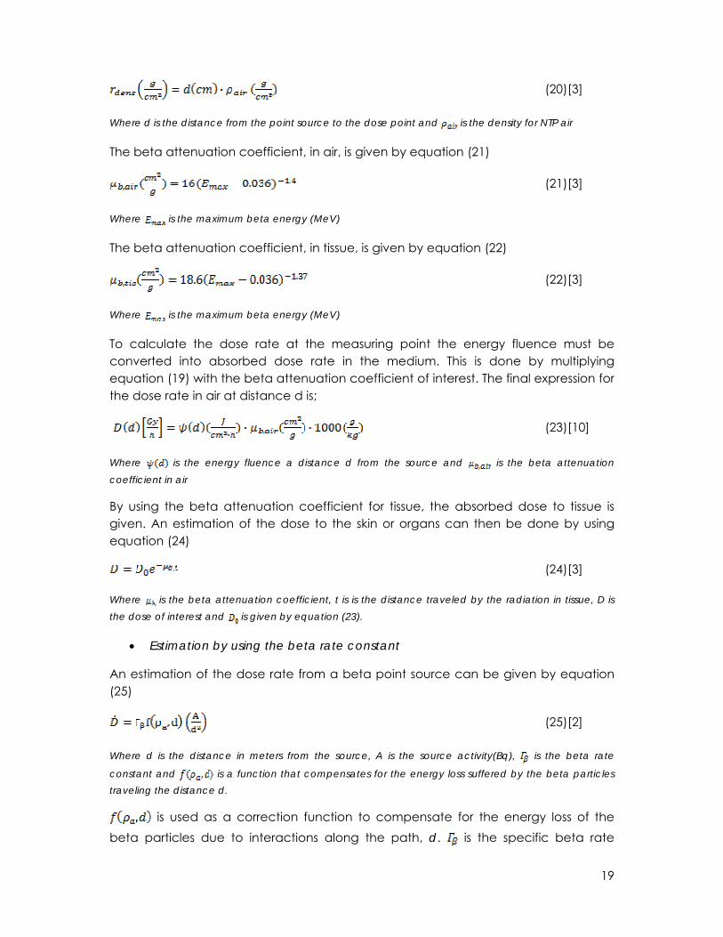
(20)[3]

Where d is the distance from the point source to the dose point and is the density for NTP air

The beta attenuation coefficient, in air, is given by equation (21)

(21)[3]

Where is the maximum beta energy (MeV)

The beta attenuation coefficient, in tissue, is given by equation (22)

(22)[3]

Where is the maximum beta energy (MeV)

To calculate the dose rate at the measuring point the energy fluence must be converted into absorbed dose rate in the medium. This is done by multiplying equation (19) with the beta attenuation coefficient of interest. The final expression for the dose rate in air at distance d is;

(23)[10]

Where is the energy fluence a distance d from the source and is the beta attenuation coefficient in air

By using the beta attenuation coefficient for tissue, the absorbed dose to tissue is given. An estimation of the dose to the skin or organs can then be done by using equation (24)

(24)[3]

Where is the beta attenuation coefficient, t is is the distance traveled by the radiation in tissue, D is the dose of interest and is given by equation (23).

• Estimation by using the beta rate constant

An estimation of the dose rate from a beta point source can be given by equation (25)

(25)[2]

Where d is the distance in meters from the source, A is the source activity(Bq), is the beta rate

constant and is a function that compensates for the energy loss suffered by the beta particles traveling the distance d.

is used as a correction function to compensate for the energy loss of the beta particles due to interactions along the path, d. is the specific beta rate

20

constant, which depends on the mean beta energy. See [2] for values of the expressions of the nuclide of interest.

5.1.2 Estimation of gamma point dose rates for calibration and constancy control sources

• Microshield

Microshield is used to calculate the effective dose (E ) (see section 2) for an isotropic geometry at the measurement point for the constancy control and calibration sources at the distances of interest.

• Approximate value by gamma rate constant

The dose rate from a gamma emitting nuclide can be estimated by equation (26)

(26)[11]

Where d is the distance from the source in meters, A is the source activity, s the gamma rate constant

5.2 Estimation of surface dose rate from waste containers

When measuring waste containers an estimation of the surface dose rate can be useful to know what dose level to expect. The estimation of the dose levels were made with the maximum allowed amount of activity, 1 , of each nuclide investigated.

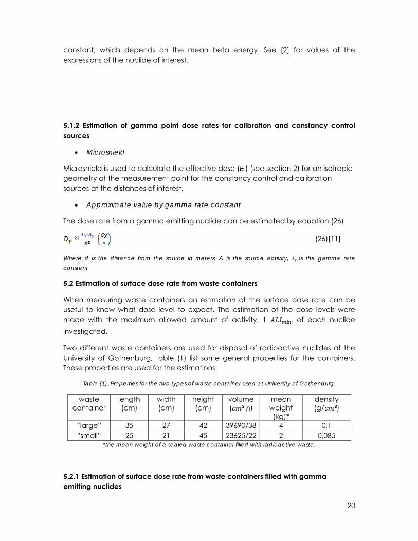
Two different waste containers are used for disposal of radioactive nuclides at the University of Gothenburg, table (1) list some general properties for the containers. These properties are used for the estimations.

Table (1). Properties for the two types of waste container used at University of Gothenburg.

waste container

length (cm)

width (cm)

height (cm)

volume ( )

mean weight (kg)*

density (g/ )

”large” 35 27 42 39690/38 4 0,1 ”small” 25 21 45 23625/22 2 0,085

*the mean weight of a sealed waste container filled with radioactive waste.

5.2.1 Estimation of surface dose rate from waste containers filled with gamma emitting nuclides

21

The surface dose rates, in air, from a gamma emitting volume source were calculated with Microshield. Three different geometries were studied. For waste containers with homogeneously distributed activity, the geometry shown in figure (8) is used. The measurement point is placed 1 cm above the center point of the top surface. This is done to better simulate a real measurement situation. For a complete description on how the source is defined in Microshield, see the appendix.

Figure(8). Geometry 1, homogeneously distributed activity. The measurement point is placed 1 cm above the surface.

For waste containers where the activity has been concentrated to the bottom half of the container and the measurement is made at the top, the geometry shown in figure (9) is used. The absorbing material is set to have the same density as the volume source, but contains no activity. The thickness of the absorber was set to 20 cm for both waste containers. The measurement point is placed 1 cm above the center point of the top surface, to better simulate a real measurement situation. For a complete description on how the source is defined, see the appendix.

22

Figure (9). Geometry 2, inhomogeneous distribution of activity. The measurement point is placed 1 cm above the surface.

For waste containers where most activity has been concentrated to one end, the geometry shown in figure (10) is used. The thickness of the source is set to 10 cm and the thickness of the absorber is set to 1 cm for both waste containers. This geometry should estimate the higher end of the spectrum of possible dose rates. The measurement point is placed 1 cm above the center point of the top surface. For a complete description on how the source is defined, see the appendix.

Figure (10). Geometry 3, concentrated distribution of activity. The measurement point is placed 1 cm above the surface.

5.2.2 Estimation of surface dose rate from waste containers filled with beta emitting nuclides

The estimation of the surface dose rate is done by calculating the dose rate by hand, no programs like Microshield for beta volume emitters were available.

For an infinitely thick volume source (source thickness beta particle range), the rate of energy absorption is equal to the energy emission for a point in the volume. This constitutes an equilibrium called ESE (energy spatial equilibrium). The dose rate inside the volume, figure (11), when conditions for ESE apply is given by equation (27).

(27)[3]

Where is the concentration of the beta emitting nuclide, tps is transformations per second, and is the mean energy (MeV) per beta particle

23

Figure(11). The dose rate for the measurement point inside the volume under ESE conditions.

Which can be reduced to equation (28)

(28)

Where is the concentration of the beta emitting nuclide and is the mean energy per beta particle

At the surface of such a volume source the energy absorption rate will be approximately half of what it is at a point within the volume, since source material will be present only on one side of the dose point, figure (12). Using equation (28), the surface dose rate can be written as;

= (29)[3]

Where is the concentration of the beta emitting nuclide and is the mean energy per beta particle

Figure (12). The surface dose rate at the measurement point from a beta emitting volume source

If the volume source emits beta radiation with different energies or if the source is made up of multiple nuclides, equation (29) can be rewritten as;

(30)[3]

Where is the number of beta particles per decay with

Equation (29) or (30) will estimate the beta dose rate at the surface of the volume source. The surface dose rates for different nuclides were calculated for the large waste container, since the larger waste container better fulfills the conditions for ESE.

24

The bremsstrahlung produced when the beta particles interact in the volume source could be included. The fraction of beta energy converted into bremsstrahlung is given by equation (31)

(31)[3]

Where is the effective atomic number of the source and is the maximum energy in MeV of the beta radiation

Bremsstrahlung is mostly of interest for the very low energy emitting nuclides, H-3 C-14, where the beta dose rate will be hard to measure due to the short range of the particles. The dose rate measured is primarily from bremsstrahlung contribution.

Estimations of bresmsstrahlung

- Approximate expression

The bremsstrahlung is set to be emitted from a virtual point in the middle of the source at a distance r form the dose point. The dose rate in air, given the conditions above, is given by equation (32)

(32)[3]

Where is the effective atomic number of the source, is the maximum energy of the beta radiation, is the linear attenuation coefficient and r is the distance from the virtual emission point to the dose point.

- Microshield

A gamma emitting source, defined according to figure (8) and equation (31), with the photon energy as the maximum energy of the beta particles could give an upper estimation of the gamma dose rate.

The result from equations (32) or Microshield can be combined with the beta dose rate to give the total surface dose.

5.3 General measurement steps used to measure constancy control and calibration sources

1. Investigate the detector for any sign of damage, to wires or to the detector itself. Check the status of the battery or power supply. If the battery level is low most monitors will not work, or if measurements are made it will give an incorrect reading. Most instruments have a built in warning system to avoid this. Refer to the instruments manual.

25

Check the monitor for a reference measurement marking, this marking should be placed facing the source at every calibration or constancy control measurement. Clear the immediate surrounding area of unnecessary objects, to reduce contribution from scattered radiation.

2 Place the detector in a jig or use some other sort of fixation at the chosen calibration distances from the source, see figure (13). This is done to keep the distance as constant as possible, and make repeated measurements easy to perform. The fixation shown on the left side of figure (13) should not be placed in a way that interferes with the radiation from the source. The fixation can, for example, be made up of a thin plastic tube. It is important that the same fixation tool is used, or that the distance is the same, when performing future measurements.

Figure (13). The measuring setup during calibration and const. control.

The distances used, for the sources, are given in table (2)

3 Measure the background radiation without the source present. If the count rate is higher than normal, it can indicate that the monitor or the surrounding

26

area is contaminated. The background radiation level should be recorded, for future references.

4 Perform a measurement with the source properly in place. Wait at least ten seconds before recording the value, some detectors might respond slowly to the radiation.

The results from step 4 can be recorded in a spread sheet program (see the appendix), that also can be used to evaluate the result and be used for future references.

5.4. Calibration method of radiation monitor instruments measuring counting rate

As mentioned in chapter 4, the manufacturer has performed an extensive investigation of the instrument. The instruments sensitivity, energy response, rate response and sensitivity to temperature variations has usually been examined. The user is usually referred to the instrument manual for any information of interest.

There are two types of calibrations that can be performed for the monitors measuring cps.

-efficiency calibration

The efficiency calibration is done to calculate the activity of the point source that is indicated as counting rate on the monitor. The calibration can be done by following the general measurement steps and recording the result from step 4. Using Equation (18), with the corrected count rate, gives the efficiency for the nuclide measured.

With known efficiency the activity of the measured radiation can be calculated with equation (18). If multiple calibration sources are available the efficiency over a wider energy spectrum can be investigated by repeating the steps 1 to 4 for each calibration source.

- Estimation of the conversion from cps to dose rate in air

A calibration concerning the conversion of counting rate to dose rate in air is done by following the same general measurement steps. The counting rate given in step 4 can be related to the calculated dose rate in air, at the measurement point for the source. The dose rate at the calibration point is given in table (2).

5.5 Constancy control method of radiation monitor instruments measuring counting rate

When performing the constancy controls, the measuring setup should be as close to identical as possible. The source is measured by following the general measurement steps.

27

If preferred, just the counting rate could be recorded. The results from the following constancy control measurements are compared with the result from the first measurement by compensating for the decay of the source, see the appendix. The results can determine if the monitor has changed its response compared to the previous constancy control measurements.

5.6 Calibration method of radiation monitoring instruments measuring dose rate

An investigation of the calibration of instruments measuring ambient dose equivalent (H*) or personal dose equivalent ( ) can be done by following the general

measurement steps and comparing the measured value with the calculated value for effective dose rate (E) at the measurement point, see table (2).

The indicated value should be higher than the calculated value for a correctly calibrated monitor, see section 2.

5.7 Constancy control of radiation monitoring instruments measuring dose rate

The source is measured by following the general measurement steps. The result from the first constancy control is recorded. For following constancy controls, the result can be related to the value of the first constancy control by compensating for the decay of the source. The results can determine if the monitor has changed its response compared to the previous constancy control measurements.

5.8 Calibration and constancy control sources

IAEA recommend that both point and surface sources are available for monitor calibrations since they make up the extremes of the measuring geometry [9], this thesis only deals with point sources.

The sources used for calibration have to be chosen carefully. The nuclide should decay in as few ways as possible, to make the measurement situation during the calibration as accurate as possible. The constancy control nuclides should have a long half-life, to make the constancy control valid over a long period of time. For convenience a single nuclide per monitor should be used.

The calibration and constancy control sources chosen are presented in table (2). All sources have a relatively long half life and have a well known decay, see the appendix.

Table(2). The constancy control sources, their activity and dose rate at the measuring point.

nuclide activity measurement distances

E ** D

, #1

176 kBq (2008-06-

01)

5 cm & 10 cm 3 µSv/h (5 cm) 0.83 µSv/h (10 cm)

4.4 µGy/h (5 cm) 1.2 µGy/h (10

cm) nuclide activity measurement

distance E ** D

28

, #2

183 MBq (2008-06-

01)

10 cm 0.87 mSv/h (10 cm) 1.26 mGy/h (10 cm)

Nuclide activity measurement distances

D

#3

211 kBq/ml (2008-05-

23)

5 cm & 10 cm No source

nuclide activity measurement distance

D

#4

37 kBq/ml 1 cm No source

*The source is a source shielded for beta contribution, see section 5. **Calculated value using Microshield, 1 mm pmma slab is placed over the source to remove the beta particle contribution.

5.5.3 Construction of calibration and constancy control sources

A point source for and has to be constructed. The sources have to be

contained in a proper way to avoid unnecessary contamination of the environment or the detector itself.

The sources should also be constructed to make sure that the dose level outside the container does not pose an unnecessary external radiation hazard.

The source has to be unshielded under measurement. Any seal would remove

the beta particles and avoid detection in the instrument. The base of the source should be constructed in aluminum to avoid the possibility that built up static electricity, generated in e.g. plastics, would be able to force the molecules to spread out and cause contamination. Aluminum has a low atomic number; this gives a low bremsstrahlung contribution.

The base of the constructed point sources is presented in figure (14)

Figure (14). The base of the source. x and y is the width, z is the thickness, d is the diameter and h is the depth of the hole.

The dimensions and material for the different sources are presented in table (3)

Table (3). The material and dimensions for the bases for the point sources that was considered.

29

material nuclide x (cm) y (cm) z (cm) d (cm) h (cm) containment aluminium 5 5 1-2 0.4 0.4 1 mm PMMA aluminium 5 5 1 0.4 0.4 N/A

The nuclides of and are in liquid solutions. An appropriate amount of the

solutions were placed in the base of the aluminum slab and left to dry, resulting in the final activity seen in table (2). The handling of the solutions was done under a closed hood.

6. Results

6.1 Dose levels around waste containers

6.1.1 Surface dose rates from gamma emitting nuclides

The results from the estimation made with Microshield are presented in table (4) and table (5) . Table (4) shows the estimations for the smaller waste container and table (5) shows the estimations for the lager waste container.

Table(4). The surface dose rates from the three different geometries estimated by Microshield for the small waste container.

Small waste container Nuclide ( ) Geometry 1

(µGy/h) Geometry 2

(µGy/h) Geometry 3

(µGy/h)

206 21 277 with buildup 220 28 297

17 1.6 24 with buildup 19 2.8 27

9.7 2.3 24.7 with buildup 10 2.6 25.3

82 11 203 with buildup 95 17 231

0.59 1.4 with buildup 0.67 1.7

1.8 0.4 4.9 with buildup 2 0.5 5.2

11 2.3 29 with buildup 12 2.6 31

with buildup

30

Table(5).The surface dose rates from the three different geometries estimated by Microshield for the large waste container.

Large waste container Nuclide ( ) Geometry 1

(µGy/h) Geometry 2

(µGy/h) Geometry 3

(µGy/h)

133 19.7 191 with buildup 146 27.5 210

11 1.5 19.5 with buildup 13 2.8 23

8.9 2.4 21 with buildup 9.4 2.7 21.6

67 11 157 with buildup 80 18 183

0.34 0.75 with buildup 0.39 0.91

1.4 0.35 3.4 with buildup 1.6 0.65 3.6

8.7 2.2 20 with buildup 9.4 2.7 22

with buildup

The results show that the smaller container has a higher surface dose rate for all nuclides, that the surface dose rate for for geometry 2 for both waste containers

are well below the legal limit (5 µGy/h) and that the surface dose rate for e.g. is

significantly above the legal limit.

Table (6) shows the results for the large waste container if the density is reduced by half.

Table(6). The large waste container with half the density, results are shown for geometry 1.

Large waste container Nuclide (ALImin) Geometry 1

(µGy/h)

9.2 with buildup 9.4

1.5 with buildup 1.6

31

As seen in table (6), the dose rate for and is almost identical with the dose

rate in table (5).

6.1.2 Surface dose rates from beta emitting nuclides

Table (7) shows the beta surface dose rates calculated for the large waste container, with the activity of 1 ALImin.

Table(7). The concentration, mean energy and surface dose rates for beta emitting nuclides in the large waste container

* Calculated using equation (32). **The sum of the two dominating beta energies. *** see [11]

Table (7) shows that the surface dose rate from the beta emitting nuclides is above the limit of 5 µGy/h for all nuclides except . The daughter nuclide of is

however .

If the mass of the waste container change, the change in dose rate will be linear (equation (30)). Due to all parameter are constant, but . A reduction in mass by 50% will lead to an increase of by a factor two.

If the mass is 2 kg for the large container, the ESE conditions are just met for the high energetic , see equation (3). Which gives a range of approximately 20 cm in the

container.

Equation (31) gives f as 0.0032 for C-14 using the effective atomic weight of 7 (approximately air). The contributions from bremsstralung is low.

Nuclide

*** *

1338

330

410

595

320

1.3

1090

0.18** 52

32

6.2 Calibration and constancy control

Table (8) shows the result for the instruments measuring the ambient dose equivalent using the general measurement steps with source #1.

Table (8).The results from the instruments measuring the ambient dose equivalent

H* instruments measured with source #1. Instrument

number Department Instrument

type Background

[µSv/h] Measured

H*(10) [µSv/h] (5 cm/10 cm)

Calculated E [µSv/h] (5 cm/10

cm)

dose error (intrinsic

error)

1 MFT** RNI 10/SR Intesimeter

0.10 3.25/1.25 3/0.83 20% [16]

2 MFT** Smart Ion 2.5 Not considered***

Not considered

Not considered

3 Dep. Of radiation physics

RNI 10/SR Intesimeter, S/N 59855

0.20 3.55/1.75 3/0.83 20% [16]



0.21 3.69/1.55 3/0.83 20% [16]


SRV-2000 0.15 3.34/1.52 3/0.83 20% [16]


Canberra Radiagem

SAC 100

0.20 3.96/* 3/0.83 15% [16]

.*The lowest recommended dose rate for measurement was 3 uSv/h, the distance 10 cm was therefore not considered. **Dep. Of Medical physics and biomedical engineering Sahlgrenska University Hospital *** due to the high background radiation value measured. c the uncertainty in positioning is also considered (estimated to 10% for 5 cm and 7% for 10 cm)

The results from table (8) show that all instruments, except instrument #2, measures a dose rate higher than the calculated effective dose at the measurement point, taking the statistical factors in mind. The instrument #2 measured a significantly high dose rate, and was therefore not considered.

Table (9) shows the results for the instruments measuring counting rate using the general measurement steps with source #1.

33

Table (9). The results for the instruments measuring cps.

Counting rate instruments measured with source #1. Department Instrument type Background

(cps) cps (5cm/10cm)

ε* (5cm)

Dair/cps (5 cm) [µGy/h cps]

MFT** Berthold LB 1210 B 9 cps 510/260 0.0033 0.0087 Dep. Of radiation physics

Miniseries 900, 44B 20 cps 500/210 0.0032 0.0092

Dep. Of radiation physics

Exploranium Gr-100 G NaI

320 2450/1419 0.014 0.0021

*calculated with equation (19) **Dep. Of Medical physics and biomedical engineering Sahlgrenska University Hospital

The result from table (9) show that the instruments are relatively insensitive to the point source, the instrument Berthold LB 1210 B and Miniseries 900 with probe 15EL should be re-measured with the beta source #3 when available.

Table (10) shows the result for the instruments measuring the ambient dose equivalent using the general measurement steps with source #2.

Table (10).The results from the instruments measuring the ambient dose equivalent.

H* instruments measured with source #2. Instrument

number Department Instrument

type Background

[µSv/h] Measured

H*(10) [mSv/h] (10 cm)

Calculated E [mSv/h] (10 cm)

dose error

(intrinsic error) c



0.21 1.22 0.87 20% [16]



0.26 1.16 0.87 20% [16]


SRV-2000 0.17 1.34 0.87 20% [16]


Canberra Radiagem

SAC 100

0.22 1.41 0.87 15% [16]

The results from table (10) shows that all the instruments indicated a measured dose rate that is higher than the calculated effective dose rate.

Table (11) shows the results for the instruments measuring cps with source #2. The source was too strong for all instruments, and not considered for the Miniseries 900, 15EL instrument.

34

Table (11). The results for the instruments measuring cps.

Counting rate instruments measured with source #2. Department Instrument type Background

(cps) cps (10cm)


Miniseries 900, 44B 25 cps overload


Miniseries 900, 15EL

3 cps -


Exploranium Gr-100 G NaI

320 overload

Result from table (8) can be summated into figure (15) for the instruments measuring the ambient dose equivalent with source #1 at 5 cm

Figure (15). The measured ambient dose equivalent for source #1 at 5 cm

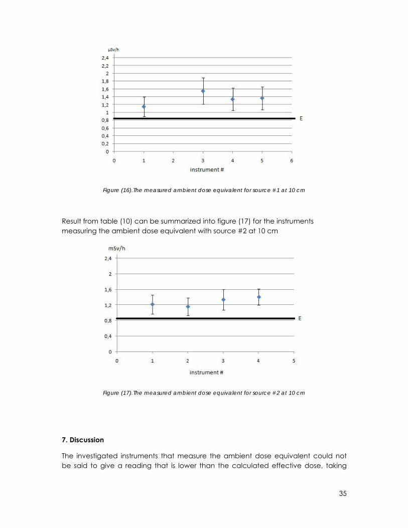
Results from table (8) can be summarized into figure (16) for the instruments measuring the ambient dose equivalent with source #1 at 10 cm

35

Figure (16).The measured ambient dose equivalent for source #1 at 10 cm

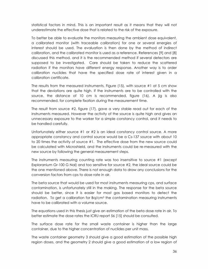
Result from table (10) can be summarized into figure (17) for the instruments measuring the ambient dose equivalent with source #2 at 10 cm

Figure (17).The measured ambient dose equivalent for source #2 at 10 cm

7. Discussion

The investigated instruments that measure the ambient dose equivalent could not be said to give a reading that is lower than the calculated effective dose, taking

36

statistical factors in mind. This is an important result as it means that they will not underestimate the effective dose that is related to the risk of the exposure.

To better be able to evaluate the monitors measuring the ambient dose equivalent, a calibrated monitor (with traceable calibration) for one or several energies of interest should be used. The evaluation is then done by the method of indirect calibration, and the calibrated monitor is used as a reference. References [9] and [8] discussed this method, and it is the recommended method if several detectors are supposed to be investigated. Care should be taken to reduce the scattered radiation if the monitors have different energy response. Another way is to order calibration nuclides that have the specified dose rate of interest given in a calibration certificate.

The results from the measured instruments, Figure (15), with source #1 at 5 cm show that the deviations are quite high. If the instruments are to be controlled with the source, the distance of 10 cm is recommended, figure (16). A jig is also recommended, for complete fixation during the measurement time.

The result from source #2, figure (17), gave a very stable read out for each of the instruments measured. However the activity of the source is quite high and gives an unnecessary exposure to the worker for a simple constancy control, and it needs to be handled carefully.

Unfortunately either source #1 or #2 is an ideal constancy control source. A more appropriate constancy and control source would be a Cs-137 source with about 10 to 20 times the activity of source #1. The effective dose from the new source could be calculated with Microshield, and the instruments could be re-measured with the new source by following the general measurement steps.

The instruments measuring counting rate was too insensitive to source #1 (except Exploranium Gr-100 G NaI) and too sensitive for source #2, the ideal source could be the one mentioned above. There is not enough data to draw any conclusions for the conversion factors from cps to dose rate in air.

The beta source that would be used for most instruments measuring cps, and surface contamination, is unfortunately still in the making. The response for the beta source should be better, since it is easier for most gas based monitors to detect the radiation. To get a calibration for Bq/cm3 the contamination measuring instruments have to be calibrated with a volume source.

The equations used in this thesis just give an estimation of the beta dose rate in air. To better estimate the dose rates the ICRU report 56 [15] should be consulted.

The surface dose rate for the small waste container is higher than the large container, due to the higher concentration of nuclides per unit mass.

The waste container geometry 3 should give a good estimation of the possible high region doses, and the geometry 2 should give a good estimation of a low region of

37

possible doses. Many calculated values are above the legal limit, it can easily be reduced just by waiting for the nuclide to decay if it has a short half life. Another way is to repackage the container into a larger container for added attenuation. A split of one waste container into two separate would also reduce the dose rate by half, given a uniform distribution.

The dose rates could also be calculated with a measurement point placed on the side on one waste container, the top point was chosen for convenience and to simulate three possible types of distributions.

The surface dose rates from the beta emitting nuclides is just a theoretical value, and will differ significantly from the measured value for the most low energetic beta radiation (especially H-3). H-3 has an extremely short range and cannot be measured with detectors like GM-tubes or proportional counters. Even C-14 will be hard to measure; most of the signal could be a result from the low bremsstrahlung contribution.

38

References

[1] Joniserande strålningens växelverkan med material, Lars Hallstadius & Sven Hertzman, radiofysiska inst., Lund, 1983 [in Swedish]

[2] The Physics of radiation protection, B Dörschel et.al, Nuclear Technology Publishing, 1996

[3] Introduction to health physics, Herman Cember, Mc Graw-Hill, Third edition, 1996

[4] Introduction to radiological physics and radiation dosimetry, Frank Herbert Attix, Wiley, 2004

[5] Dosbestämning I strålskyddsarbete, Lennart Lindborg, SSI, Strålskyddsnytt nr 4, 1998 [in Swedish]

[6] Radiation detection and measurement, Glenn F Knoll, Wiley, Third edition, 1999

[7] Grundläggande strålningsfysik, Mats Isaksson, Studentlitteratur, 2002 [in Swedish]

[8] An introduction to radiation protection, Alan Martin & Sam Harbison, Hoder Arnold, Fifth edition, 2006

[9] IAEA Safety report series no 16, Calibration of radiation protection monitoring instruments, 2000

[10] Health Physics Society, especially http://www.hps.org/publicinformation/ate/q3896.pdf, visited in 050508

[11] Strålskydd, Curt Bergman et.al., natur och kultur, 1988 [in Swedish]

[12] SSI FS 2000:7, Statens strålskyddsinstituts föreskrifter om laboratorieverksamhet med radioaktiva ämnen i form av öppna strålkällor, SSI, 2000 [in Swedish] [13] SSI FS 1983:7, Statens strålskyddsinstituts föreskrifter m.m. om icke kärnenergianknutet radioaktivt avfall, SSI, 1983 [in Swedish] [14] ICRP 30, Limits for the Intake of Radionuclides by Workers, ICRP, 1978

[15] ICRU 56, Dosimetry of External Beta Rays for Radiation Protection, ICRU, 1997

[16] Inventory of Radiation Monitors at Göteborg University and development of control and calibration protocol, Elen Monsen, Master Thesis, Department of radiation physics, University of Gothenburg, 2007

[17] Radiation safety manual, office of radiation, chemical and biological safety, Michigan state university, 1996 [18] The Lund/LBNL Nuclear Data Search, http://nucleardata.nuclear.lu.se/nucleardata/toi/, visited in 051408

39

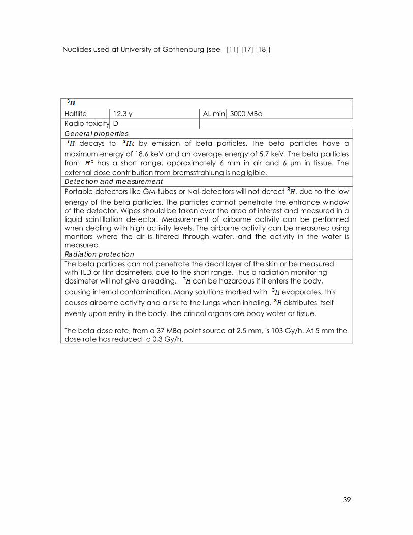
Nuclides used at University of Gothenburg (see [11] [17] [18])

Halflife 12.3 y ALImin 3000 MBq Radio toxicity D General properties

decays to by emission of beta particles. The beta particles have a maximum energy of 18.6 keV and an average energy of 5.7 keV. The beta particles from has a short range, approximately 6 mm in air and 6 µm in tissue. The external dose contribution from bremsstrahlung is negligible. Detection and measurement Portable detectors like GM-tubes or NaI-detectors will not detect , due to the low energy of the beta particles. The particles cannot penetrate the entrance window of the detector. Wipes should be taken over the area of interest and measured in a liquid scintillation detector. Measurement of airborne activity can be performed when dealing with high activity levels. The airborne activity can be measured using monitors where the air is filtered through water, and the activity in the water is measured. Radiation protection The beta particles can not penetrate the dead layer of the skin or be measured with TLD or film dosimeters, due to the short range. Thus a radiation monitoring dosimeter will not give a reading. can be hazardous if it enters the body, causing internal contamination. Many solutions marked with evaporates, this causes airborne activity and a risk to the lungs when inhaling. distributes itself evenly upon entry in the body. The critical organs are body water or tissue. The beta dose rate, from a 37 MBq point source at 2.5 mm, is 103 Gy/h. At 5 mm the dose rate has reduced to 0,3 Gy/h.

40

Halflife 5730 y ALImin 97 MBq Radio toxicity C General properties

decay to by emission of beta particles. The beta particles have a maximum energy of 156 keV and an average energy of 49 keV. The range from the beta particles is approximately 24 cm in air and 0,3 mm in tissue. The photon contribution from bremsstrahlung is negligible Detection and measurement Measurement can be done with a GM-tube fitted with a thin entrance window, the measurement must be performed at close range, ca 1 cm. Wipes taken from the area of interest can be measured in a liquid scintillation detector. Radiation protection Due to the short range of the beta particles, radiation monitoring dosimeters will not give a reading and 1% of the beta particles can penetrate the dead layer of the skin. is not significantly volatile at room temperature. is hazardous if it enters the body causing internal contamination. Inhalation of airborne activity or absorption through the skin is a large risk. The critical organs are fat tissue or bone. In dealing with activity levels (above 40 MBq) should be handled under a closed hood. Checking for contamination is important. With its long half-life, it can cause a waste management problem. The beta dose rate, from a 37 MBq point source at 1 cm, is 12,4 Gy/h. At 2 cm the dose rate has reduced to 2,5 Gy/h.

41

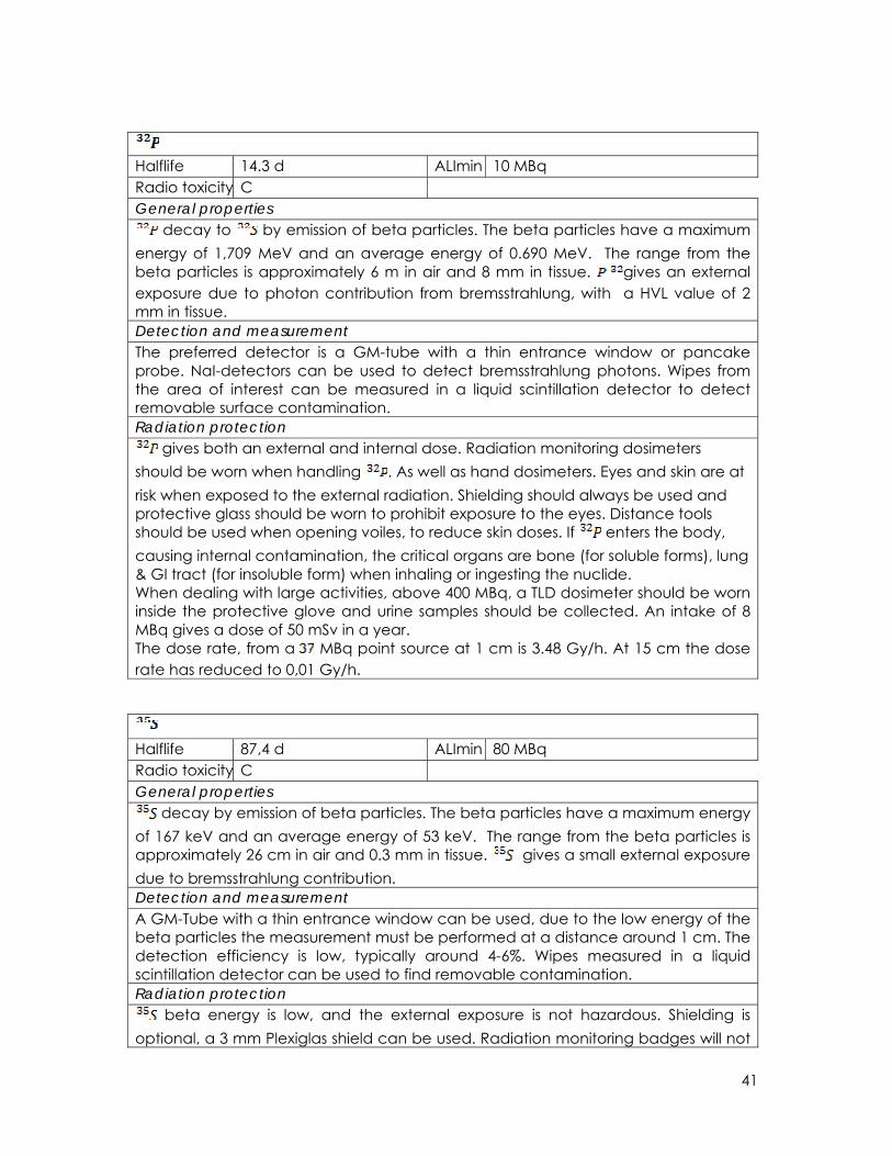
Halflife 14.3 d ALImin 10 MBq Radio toxicity C General properties

decay to by emission of beta particles. The beta particles have a maximum energy of 1,709 MeV and an average energy of 0.690 MeV. The range from the beta particles is approximately 6 m in air and 8 mm in tissue. gives an external exposure due to photon contribution from bremsstrahlung, with a HVL value of 2 mm in tissue. Detection and measurement The preferred detector is a GM-tube with a thin entrance window or pancake probe. NaI-detectors can be used to detect bremsstrahlung photons. Wipes from the area of interest can be measured in a liquid scintillation detector to detect removable surface contamination. Radiation protection

gives both an external and internal dose. Radiation monitoring dosimeters should be worn when handling . As well as hand dosimeters. Eyes and skin are at risk when exposed to the external radiation. Shielding should always be used and protective glass should be worn to prohibit exposure to the eyes. Distance tools should be used when opening voiles, to reduce skin doses. If enters the body, causing internal contamination, the critical organs are bone (for soluble forms), lung & GI tract (for insoluble form) when inhaling or ingesting the nuclide. When dealing with large activities, above 400 MBq, a TLD dosimeter should be worn inside the protective glove and urine samples should be collected. An intake of 8 MBq gives a dose of 50 mSv in a year. The dose rate, from a MBq point source at 1 cm is 3.48 Gy/h. At 15 cm the dose rate has reduced to 0,01 Gy/h.

Halflife 87,4 d ALImin 80 MBq Radio toxicity C General properties

decay by emission of beta particles. The beta particles have a maximum energy of 167 keV and an average energy of 53 keV. The range from the beta particles is approximately 26 cm in air and 0.3 mm in tissue. gives a small external exposure due to bremsstrahlung contribution. Detection and measurement A GM-Tube with a thin entrance window can be used, due to the low energy of the beta particles the measurement must be performed at a distance around 1 cm. The detection efficiency is low, typically around 4-6%. Wipes measured in a liquid scintillation detector can be used to find removable contamination. Radiation protection

beta energy is low, and the external exposure is not hazardous. Shielding is optional, a 3 mm Plexiglas shield can be used. Radiation monitoring badges will not

42

give a reading, due to the low energetic beta particles. 12% of the beta radiation can penetrate the dead layer of the skin. If enters the body, causing internal contamination, the critical organs are the testis. The beta dose rate, from a Bq point source at 1 cm, is 11.7 Gy/h. At 2.5 cm the dose rate has reduced to 0,94 Gy/h.

Halflife 27.8 d ALImin 700 MBq Radio toxicity C General properties

decay by photon and beta emisson. The dominating beta energy has a maximum energy of 752 keV. The dominating gamma energy has a energy of 320 keV. Detection and measurement The preferred detector of choice is a liquid scintillation detector, for example a NaI-detector. GM-tubes or similar detectors are very inefficient at detecting due to the low photon energies emitted. Wipes measured in liquid scintillation detectors can be used to detect removable surface contamination. Radiation protection Personal radiation monitoring dosimeters should be worn, both whole body and extremity detector badges. Shielding should always be used. A 5 mm lead plate will reduce the dose rate significantly. If enters the body, causing internal contamination, it enriches in the lower large intestine. The dose rate, from a 37 MBq point source at 1 cm, is 1.6 Gy/h. At 10 cm the dose rate has reduced to 0,02 Gy/h.

Halflife 64 h ALImin 20 MBq Radio toxicity B General properties

decay by emission of beta particles. The beta particles have a maximum energy of 2.27 MeV and an average energy of 0.76 MeV. The range from the beta particles is approximately 1000 cm in air and 1 cm in tissue. Detection and measurement GM-tube Radiation protection Dose rate from a 37 MBq point source at 1 cm is 6.77 Gy/h

Halflife 13.3 h ALImin 100 MBq Radio toxicity C General properties decay by emission of positron and gamma radiation. The beta (positron) particles

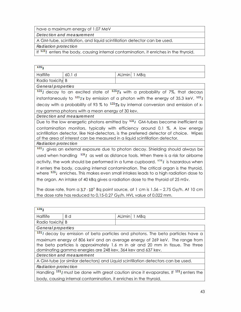
43

have a maximum energy of 1.07 MeV Detection and measurement A GM-tube, scintillation, and liquid scintillation detector can be used. Radiation protection If enters the body, causing internal contamination, it enriches in the thyroid.

Halflife 60.1 d ALImin 1 MBq Radio toxicity B General properties

decay to an excited state of with a probability of 7%, that decays instantaneously to by emission of a photon with the energy of 35.3 keV. decay with a probability of 93 % to by internal conversion and emission of x-ray gamma photons with a mean energy of 30 kev. Detection and measurement Due to the low energetic photons emitted by GM-tubes become inefficient as contamination monitors, typically with efficiency around 0.1 %. A low energy scintillation detector, like NaI-detectors, is the preferred detector of choice. Wipes of the area of interest can be measured in a liquid scintillation detector. Radiation protection

gives an external exposure due to photon decay. Shielding should always be used when handling as well as distance tools. When there is a risk for airborne activity, the work should be performed in a fume cupboard. is hazardous when it enters the body, causing internal contamination. The critical organ is the thyroid, where enriches. This makes even small intakes leads to a high radiation dose to the organ. An intake of 40 kBq gives a radiation dose to the thyroid of 25 mSv. The dose rate, from a Bq point source, at 1 cm is 1.56 – 2.75 Gy/h. At 10 cm the dose rate has reduced to 0,15-0.27 Gy/h. HVL value of 0.022 mm.

Halflife 8 d ALImin 1 MBq Radio toxicity B General properties

decay by emission of beta particles and photons. The beta particles have a maximum energy of 806 keV and an average energy of 269 keV. The range from the beta particles is approximately 1.6 m in air and 20 mm in tissue. The three dominating gamma energies are 248 kev, 364 kev and 637 kev. Detection and measurement A GM-tube (or similar detectors) and Liquid scintillation detectors can be used. Radiation protection Handling must be done with great caution since it evaporates. If enters the body, causing internal contamination, it enriches in the thyroid.

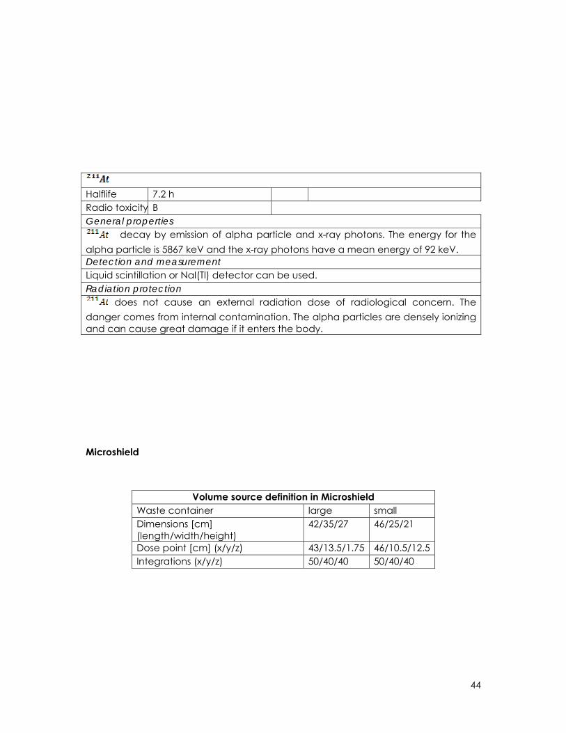
44

Halflife 7.2 h Radio toxicity B General properties

decay by emission of alpha particle and x-ray photons. The energy for the alpha particle is 5867 keV and the x-ray photons have a mean energy of 92 keV. Detection and measurement Liquid scintillation or NaI(Tl) detector can be used. Radiation protection

does not cause an external radiation dose of radiological concern. The danger comes from internal contamination. The alpha particles are densely ionizing and can cause great damage if it enters the body.

Microshield

Volume source definition in Microshield Waste container large small Dimensions [cm] (length/width/height)

42/35/27 46/25/21

Dose point [cm] (x/y/z) 43/13.5/1.75 46/10.5/12.5 Integrations (x/y/z) 50/40/40 50/40/40

Spread sheet results

Första kontrollen Efterföljande kontroll Datum 2008-06-03 Datum 2009-06-03 Avdelning: Radiofysik Instrument: RNI 10/SR Dagar sedan Intensimeter första kontrollen: 365 S/N 59855 Dosfel: (se tabell) 20% Mätt bakgrund 0,2 Sönderfallskorrigerat mätutslag 1,51 Källa nr: 1 Mätavstånd 10 cm Instrumentet bör ha ett mätutslag som ligger mellan (95 % konfidens intervall) 1,10 och 1,93 Steg 1 (OK/EJ OK) Ok Steg 2 (OK/beskriv fixeringen) Ok, fixerad i hållare på 10 cm Steg 3 (Indikerad bakgrund) 0,2 Steg 4 (indikerad dosrat) 1,75 Mätt dosrat (uSv/h) 1,55

Första kontrollen Efterföljande kontroll Datum 2008-06-03 Datum 2009-06-03 Avdelning: Radiofysik Instrument: RNI 10/SR Dagar sedan Intensimeter första kontrollen: 365 S/N 59857 Dosfel: (se manual) 20% Mätt bakgrund 0,21 Sönderfallskorrigerat mätutslag 1,31 Källa nr: 1 Mätavstånd 10 cm Instrumentet bör ha ett mätutslag som ligger mellan (95% koinf. intervall) 0,90 och 1,72 Steg 1 (OK/EJ OK) Ok Steg 2 (OK/beskriv fixeringen) Ok, fixerad i hållare på 10 cm Steg 3 (Indikerad bakgrund) 0,21 Steg 4 (indikerad dosrat) 1,55 Mätt dosrat (uSv/h) 1,34

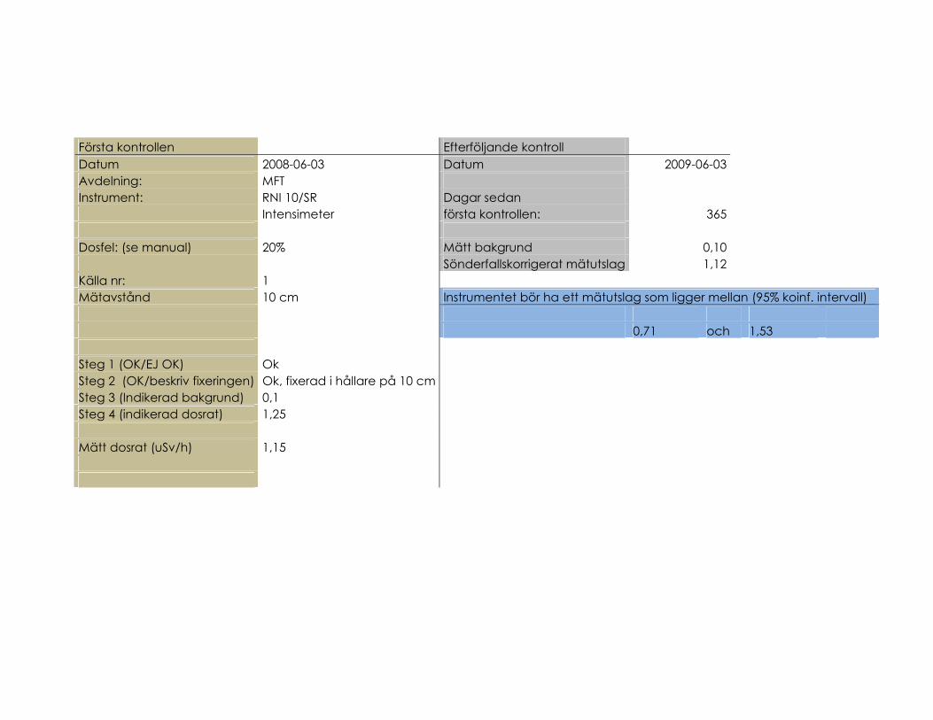
Första kontrollen Efterföljande kontroll Datum 2008-06-03 Datum 2009-06-03 Avdelning: MFT Instrument: RNI 10/SR Dagar sedan Intensimeter första kontrollen: 365 Dosfel: (se manual) 20% Mätt bakgrund 0,10 Sönderfallskorrigerat mätutslag 1,12 Källa nr: 1 Mätavstånd 10 cm Instrumentet bör ha ett mätutslag som ligger mellan (95% koinf. intervall) 0,71 och 1,53 Steg 1 (OK/EJ OK) Ok Steg 2 (OK/beskriv fixeringen) Ok, fixerad i hållare på 10 cm Steg 3 (Indikerad bakgrund) 0,1 Steg 4 (indikerad dosrat) 1,25 Mätt dosrat (uSv/h) 1,15

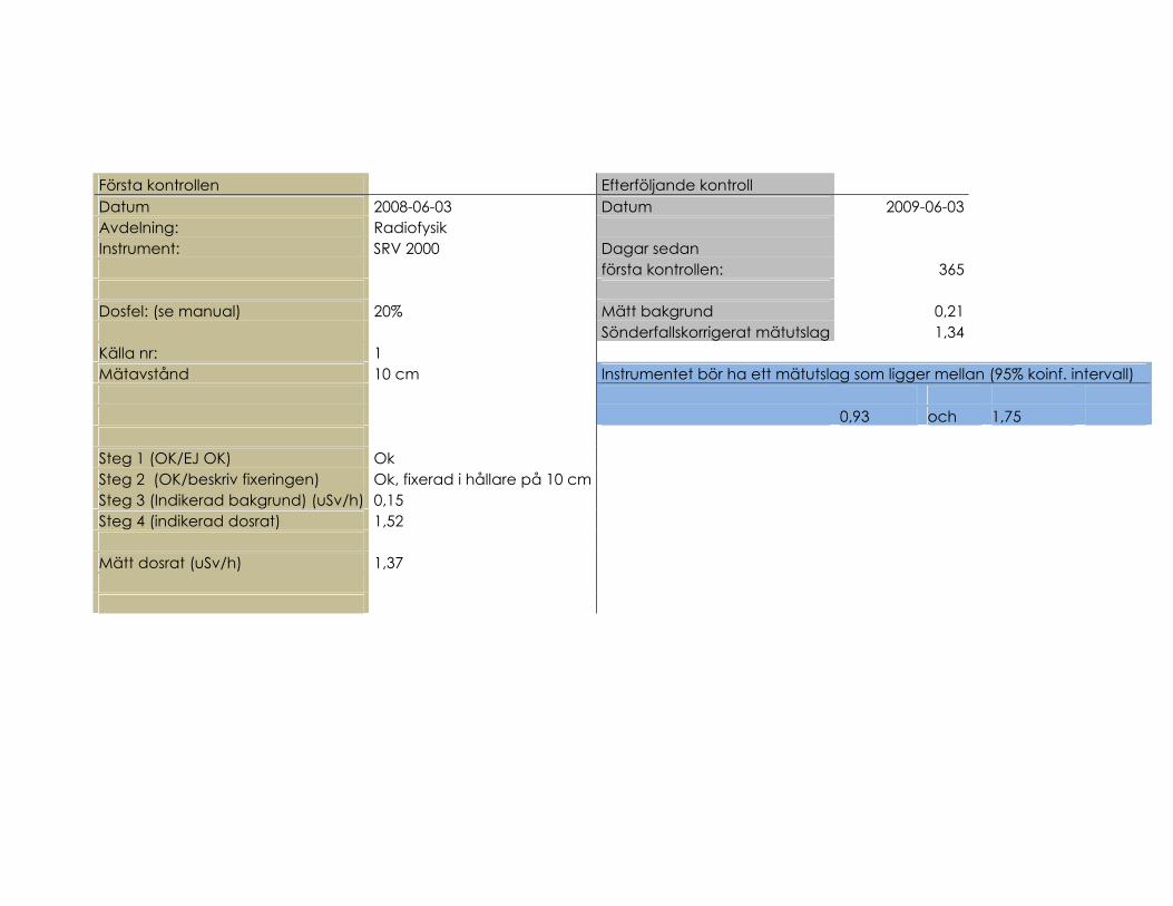
Första kontrollen Efterföljande kontroll Datum 2008-06-03 Datum 2009-06-03 Avdelning: Radiofysik Instrument: SRV 2000 Dagar sedan första kontrollen: 365 Dosfel: (se manual) 20% Mätt bakgrund 0,21 Sönderfallskorrigerat mätutslag 1,34 Källa nr: 1 Mätavstånd 10 cm Instrumentet bör ha ett mätutslag som ligger mellan (95% koinf. intervall) 0,93 och 1,75 Steg 1 (OK/EJ OK) Ok Steg 2 (OK/beskriv fixeringen) Ok, fixerad i hållare på 10 cm Steg 3 (Indikerad bakgrund) (uSv/h) 0,15 Steg 4 (indikerad dosrat) 1,52 Mätt dosrat (uSv/h) 1,37

Första kontrollen Efterföljande kontroll Datum 2008-06-03 Datum 2009-06-03 Avdelning: Radiofysik Instrument: RNI 10/SR Dagar sedan Intensimeter första kontrollen: 365 S/N 59855 Dosfel: (se manual) 20% Mätt bakgrund 0,2 Sönderfallskorrigerat mätutslag 1,19 Källa nr: 2 Mätavstånd 10 cm Instrumentet bör ha ett mätutslag som ligger mellan (95% koinf. intervall) 0,78 och 1,60 Steg 1 (OK/EJ OK) Ok Steg 2 (OK/beskriv fixeringen) Ok, fixerad i hållare på 10 cm Steg 3 (Indikerad bakgrund) (uSv/h) 0,21 Steg 4 (indikerad dosrat) (mSv/h) 1,22 Mätt dosrat (mSv/h) 1,22

Första kontrollen Efterföljande kontroll Datum 2008-06-03 Datum 2009-06-03 Avdelning: Radiofysik Instrument: RNI 10/SR Dagar sedan Intensimeter första kontrollen: 365 S/N 59857 Dosfel: (se manual) 20% Mätt bakgrund 0,2 Sönderfallskorrigerat mätutslag 1,13 Källa nr: 2 Mätavstånd 10 cm Instrumentet bör ha ett mätutslag som ligger mellan (95% koinf. intervall) 0,72 och 1,54 Steg 1 (OK/EJ OK) Ok Steg 2 (OK/beskriv fixeringen) Ok, fixerad i hållare på 10 cm Steg 3 (Indikerad bakgrund) (uSv/h) 0,26 Steg 4 (indikerad dosrat) (mSv/h) 1,16 Mätt dosrat (mSv/h) 1,16

Första kontrollen Efterföljande kontroll Datum 2008-06-03 Datum 2009-06-03 Avdelning: Radiofysik Instrument: SRV-2000 Dagar sedan första kontrollen: 365 Dosfel: (se manual) 20% Mätt bakgrund 0,17 Sönderfallskorrigerat mätutslag 1,31 Källa nr: 2 Mätavstånd 10 cm Instrumentet bör ha ett mätutslag som ligger mellan (95% koinf. intervall) 0,90 och 1,72 Steg 1 (OK/EJ OK) Ok Steg 2 (OK/beskriv fixeringen) Ok, fixerad i hållare på 10 cm Steg 3 (Indikerad bakgrund) (uSv/h) 0,17 Steg 4 (indikerad dosrat) (mSv/h) 1,34 Mätt dosrat (mSv/h) 1,34

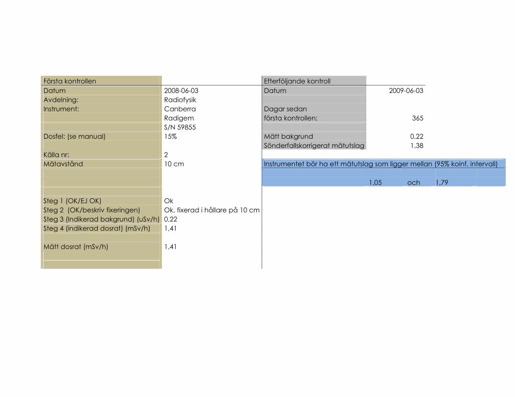
Första kontrollen Efterföljande kontroll Datum 2008-06-03 Datum 2009-06-03 Avdelning: Radiofysik Instrument: Canberra Dagar sedan Radigem första kontrollen: 365 S/N 59855 Dosfel: (se manual) 15% Mätt bakgrund 0,22 Sönderfallskorrigerat mätutslag 1,38 Källa nr: 2 Mätavstånd 10 cm Instrumentet bör ha ett mätutslag som ligger mellan (95% koinf. intervall) 1,05 och 1,79 Steg 1 (OK/EJ OK) Ok Steg 2 (OK/beskriv fixeringen) Ok, fixerad i hållare på 10 cm Steg 3 (Indikerad bakgrund) (uSv/h) 0,22 Steg 4 (indikerad dosrat) (mSv/h) 1,41 Mätt dosrat (mSv/h) 1,41

Development of Constancy Control and Calibration Protocols for

Documents

Transcript of Development of Constancy Control and Calibration Protocols for