DEVELOPMENT OF BOLTED FLANGE DESIGN TOOL BASED ON...

DEVELOPMENT OF BOLTED FLANGE DESIGN TOOL BASED ON FINITE

ELEMENT ANALYSIS AND ARTIFICIAL NEURAL NETWORK

A THESIS SUBMITTED TO

THE GRADUATE SCHOOL OF NATURAL AND APPLIED SCIENCES

OF

MIDDLE EAST TECHNICAL UNIVERSITY

BY

ALPER YILDIRIM

IN PARTIAL FULFILLMENT OF THE REQUIREMENTS

FOR

THE DEGREE OF MASTER OF SCIENCE

IN

AEROSPACE ENGINEERING

SEPTEMBER 2015

Approval of the thesis:

DEVELOPMENT OF BOLTED FLANGE DESIGN TOOL BASED ON

FINITE ELEMENT ANALYSIS AND ARTIFICIAL NEURAL NETWORK

submitted by ALPER YILDIRIM in partial fulfillment of the requirements for the

degree of Master of Science in Aerospace Engineering Department, Middle East

Technical University by,

Prof. Dr. Gülbin Dural Ünver ____________

Dean, Graduate School of Natural and Applied Sciences

Prof. Dr. Ozan Tekinalp ____________

Head of Department, Aerospace Engineering

Prof. Dr. Altan Kayran ____________

Supervisor, Aerospace Engineering Dept., METU

Examining Committee Members:

Asst. Prof. Dr. Ercan Gürses ____________

Aerospace Engineering Dept., METU

Prof. Dr. Altan Kayran ____________


Asst. Prof. Dr. Tuncay Yalçınkaya ____________


Assoc.Prof. Dr. Demirkan Çöker ____________


Asst. Prof. Dr. Cihan Tekoğlu ____________

Mechanical Engineering Dept., TOBB ETÜ

Date: 03.09.2015

iv

I hereby declare that all information in this document has been obtained and

presented in accordance with academic rules and ethical conduct. I also declare

that, as required by these rules and conduct, I have fully cited and referenced all

material and results that are not original to this work.

Name, Last name: Alper YILDIRIM

Signature :

v

ABSTRACT

DEVELOPMENT OF BOLTED FLANGE DESIGN TOOL BASED ON

FINITE ELEMENT ANALYSIS AND ARTIFICIAL NEURAL NETWORK

Yıldırım, Alper

M. S., Department of Aerospace Engineering

Supervisor: Prof. Dr. Altan Kayran

September 2015, 117 pages

In bolted flange connections, commonly utilized in aircraft engine designs, structural

integrity and minimization of the weight are achieved by the optimum combination of

the design parameters utilizing the outcome of many structural analyses. Bolt size,

number of bolts, bolt locations, casing thickness, flange thickness, bolt preload, and

axial external force are some of the critical design parameters in bolted flange

connections. Theoretical analysis and finite element analysis (FEA) are two main

approaches to perform the structural analysis of the bolted flange connection.

Theoretical approaches require the simplification of the geometry and are generally

over safe. In contrast, finite element analysis is more reliable but at the cost of high

computational power. In this work, the methodology developed for the iterative

analyses of bolted flange utilizes artificial neural network approximation of FEA

database formed with more than ten thousands of non-linear analyses involving

contact. In the design tool, the structural analysis database is created by combining

parametric variables by each other. The number of intervals for each variable in the

upper and lower range of the variables has been determined with the parameters

correlation study in which the significance of parameters are evaluated. As a follow-

up study, the design tool is compared with FEA and the theoretical approach of ESDU.

vi

Keywords: Bolted Flange Connection, Artificial Neural Network, Parameters

Correlation, Finite Element Analysis

vii

ÖZ

CİVATALI FLANŞ TASARIM ARACININ SONLU ELEMANLAR

ANALİZİ VE YAPAY SİNİR AĞI İLE GELİŞTİRİLMESİ

Yıldırım, Alper

Yüksek Lisans, Havacılık ve Uzay Mühendisliği Bölümü

Tez Yöneticisi: Prof. Dr. Altan Kayran

Eylül 2015, 117 sayfa

Uçak motoru tasarımlarda sıkça kullanılmakta olan cıvatalı flanş bağlantılarında

yapısal bütünlüğün korunması ve ağırlığın azaltılması, yapısal analizlerin sonuçlarına

dayanarak tasarım değişkenlerinin en uygun birleşimi seçilerek sağlanır. Civatalı flanş

bağlantılarında, cıvata boyutu, cıvata sayısı, cıvata pozisyonu, kılıf kalınlığı, flanş

kalınlığı, cıvata önyüklemesi ve eksenel dış kuvvet kritik tasarım değişkenleridir.

Teorik analiz ve sonlu elemanlar analizi cıvatalı flanş bağlantılarının yapısal

analizlerinde kullanılan iki temel analiz yöntemidir. Teorik yaklaşım geometrinin

basitleştirilmesini gerektirir ve genellikle gereğinden fazla emniyetli sonuç verir. Öte

yandan sonlu elemanlar analizi daha doğru sonuçlar verir, fakat daha uzun hesaplama

süresi gerektirir. Bu çalışmada, cıvatalı flanş bağlantılarının tekrarlı analizlerine

yönelik geliştirilmiş olan yöntem, on binden fazla doğrusal olmayan, kontak içeren

sonlu elemanlar analiz sonucunun oluşturduğu yapay sinir ağını kullanır. Bu tasarım

aracında, yapısal analizleri içeren veri tabanı, parametrik değişkenlerin birbirleri ile

kombine edilmesiyle oluşur. Parametrik değişkenlerin her birinin girdi sayısı,

parametre korelasyonu çalışması ile parametrelerin etkisi değerlendirilerek belirlenir.

Bu çalışmanın devamında, geliştirilen tasarım aracı sonlu elemanlar analizi yöntemi

ve ESDU teorik yaklaşımıyla karşılaştırılır.

viii

Anahtar Kelimeler: Civatalı Flanş Bağlantısı, Yapay Sinir Ağı, Parametre

Korelasyonu, Sonlu Elemanlar Analizi

ix

To my mother, father, sister, and lovely one

x

ACKNOWLEDGEMENTS

The author would like to express his sincere gratitude to his supervisor Prof. Dr. Altan

Kayran for his advice, criticism, and excellent guidance throughout the study.

The author also thanks to Assist. Prof. Dr. Ercan Gürses and Assoc. Prof. Dr.

Demirkan Çöker for their decent contributions to this study.

The author has been supported by ASELSAN A.S. from the beginning to the end of

this period and feels thankful for all the contributions by ASELSAN A.S.

The author has been supported by The Scientific and Technological Research Council

of Turkey (TÜBİTAK) as a scholarship student of the support program “BİDEB 2210-

A Genel Yurt İçi Yüksek Lisans Burs Programı”. The author would like to take this

occasion to deeply thank for this support.

There are many people who have significantly helped to this study so far; therefore,

the author feels glad about the contribution of each one of them, whose names are not

written here.

xi

TABLE OF CONTENTS

ABSTRACT ................................................................................................................ v

ÖZ… ......................................................................................................................... vii

ACKNOWLEDGEMENTS ........................................................................................ x

TABLE OF CONTENTS ........................................................................................... xi

LIST OF TABLES ................................................................................................... xiii

LIST OF FIGURES .................................................................................................. xv

LIST OF SYMBOLS AND ABBREVIATIONS .................................................... xix

CHAPTERS

1. INTRODUCTION ............................................................................................... 1

2. SCOPE OF THE THESIS ................................................................................. 13

3. FINITE ELEMENT ANALYSIS OF BOLTED FLANGE CONNECTION .... 17

3.1 Analysis Geometry and Meshing .............................................................. 18

3.1.1 Bolted Flange Connection Assembly .................................................. 18

3.1.2 Bolt-Nut Geometry.............................................................................. 24

3.1.3 Flange Geometry ................................................................................. 28

3.1.4 Washer Geometry................................................................................ 30

3.1.5 Mesh Quality ....................................................................................... 31

3.2 Material and Contact Details ..................................................................... 31

3.3 Load and Boundary Conditions ................................................................ 33

3.4 Analysis Properties ................................................................................... 34

3.5 Finite Element Solution of the Bolted Flange Connection ....................... 35

3.6 Case Studies .............................................................................................. 43

3.6.1 Comparison of Mesh Sizes.................................................................. 44

3.6.2 Comparison of Meshes with Linear and Quadratic Elements ............. 46

3.6.3 Comparison of Small Deflection and Large Deflection Analysis ....... 47

3.6.4 Comparison of Effective Bolt and Nut Diameter on the Results ........ 48

xii

4. PARAMETERS CORRELATION STUDY ...................................................... 49

4.1 Theory ....................................................................................................... 49

4.2 Method....................................................................................................... 51

4.3 Results of Parameters Correlations ........................................................... 57

5. ARTIFICIAL NEURAL NETWORK APPROXIMATION ............................. 65

5.1 Theory ....................................................................................................... 65

5.2 The Artificial Neural Network Generation Process .................................. 68

5.3 Results of the Artificial Neural Network .................................................. 72

6. RESULTS AND EVALUATION ...................................................................... 75

6.1 Comparison with Finite Element Analysis ................................................ 76

6.2 Comparison with Theoretical Approach ................................................... 80

7. CONCLUSION AND FUTURE WORKS ........................................................ 93

7.1 Conclusion ................................................................................................. 93

7.2 Future Works ............................................................................................. 95

REFERENCES .......................................................................................................... 97

APPENDICES

A. INSTRUCTIONS TO PREPARE ARTIFICIAL NEURAL NETWORK FOR

THE BOLTED FLANGE DESIGN TOOL ............................................................ 101

B. THE ARTIFICIAL NEURAL NETWORK SETUP SCRIPT ......................... 113

C. SUPPLEMENTARY CHARTS ....................................................................... 117

xiii

LIST OF TABLES

TABLES

Table 3.1 The nominal values of the parameters in the analysis model ................... 22

Table 3.2 Material properties used in the analysis model [7] ................................... 32

Table 3.3 Materials of the components in analysis model ........................................ 32

Table 3.4 Contact details of the analysis model according to Figure 3.16 ............... 33

Table 3.5 The corresponding tensile stress area values for each bolt type ............... 43

Table 3.6 The comparison of five different mesh sizes in analyses.......................... 46

Table 3.7 The effect of mid-side nodes on the analysis results ................................ 47

Table 3.8 The comparison of the large deflection behavior and the small deflection

behavior in the analysis model .................................................................................. 48

Table 3.9 The comparison of the effect of effective bolt diameter size on the

results…... ................................................................................................................. 48

Table 4.1 Sample problem data of Spearman’s rank correlation .............................. 51

Table 4.2 The nominal values, upper and lower limits of all input parameters ........ 56

Table 4.3 Bolt pretension and axial force values for each analysis set ..................... 57

Table 4.4 The correlation matrix of parametric set-1 ............................................... 60

Table 4.5 The input values for the input parameters to be used in the main parametric

study .......................................................................................................................... 63

Table 4.6 The correlation values for the remaining parametric sets as well as the main

parametric set in reference to Table 4.3…………………………………..………………….64

Table 6.1 Test set-1, (the samples are selected from the training points) ................. 76

Table 6.2 The results of test set-1, (the samples are selected from the training

points)………. ........................................................................................................... 77

Table 6.3 Test set-2, (the samples are in between the training points) ..................... 78

xiv

Table 6.4 The results of test set-2, (the samples are in between the training points) 79

Table 6.5 Test set-3, (extrapolation, the painted cells indicate the values outside the

training limits) ........................................................................................................... 79

Table 6.6 The results of test set-3 (extrapolation) ..................................................... 80

Table 6.7 The results of the sample problems with and without separation solved by

theoretical approach, FEA, and the developed tool................................................... 91

Table A.1 Limits of the input parameters for parametric analyses and ANN

training……............................................................................................................. 109

Table A.2 The parametric input values for each variable in the parametric

analyses…… ........................................................................................................... 109

xv

LIST OF FIGURES

FIGURES

Figure 1.1 A bolted flange connection sample............................................................ 2

Figure 1.2 A regular linear tetrahedral element with four nodes ................................ 4

Figure 1.3 A regular quadratic tetrahedral element with ten nodes ............................ 4

Figure 1.4 A regular linear hexahedral element with eight nodes .............................. 5

Figure 1.5 A regular quadratic hexahedral element with twenty nodes ...................... 5

Figure 2.1 Flowchart of the bolted flange design tool development procedure........ 15

Figure 3.1 Circular bolted flange connection geometry............................................ 19

Figure 3.2 Cross-sectional view of the bolted flange connection geometry with the

components ............................................................................................................... 19

Figure 3.3 Axisymmetric bolted flange sector model ............................................... 20

Figure 3.4 The circular sector analysis model with the geometric parameters ......... 21

Figure 3.5 Sectional analysis geometry of the circular bolted flange connection .... 23

Figure 3.6 Cross section view of the meshed geometry............................................ 23

Figure 3.7 The united analysis model of the bolt and the nut with the cylindrical outer

geometries ................................................................................................................. 25

Figure 3.8 The imaginary circles and the effective circle to calculate the effective

diameter of the bolt head and the nut ........................................................................ 26

Figure 3.9 Edge sizing of bolt-nut body ................................................................... 27

Figure 3.10 The angle of flange section used in the analysis .................................... 28

Figure 3.11 The variable distance of bolt hole to center axis nominated as Radius

C……. ....................................................................................................................... 28

Figure 3.12 The multizone source surfaces painted in red of the flange .................. 29

xvi

Figure 3.13 The opposite multizone source surfaces painted in red of the flange .... 29

Figure 3.14 Edge sizing of the circular sector flange body with the mesh structure. 30

Figure 3.15 Edge sizing of the washer ...................................................................... 31

Figure 3.16 Representations of the contacts on the cross-sectional bolted flange

connection view ......................................................................................................... 33

Figure 3.17 Load and boundary conditions; the fixed end on the right and the external

force applied on the left ............................................................................................. 34

Figure 3.18 Load and boundary conditions: the designated lateral surfaces of the

analysis geometry ...................................................................................................... 34

Figure 3.19 Equivalent Von Mises stress distribution in flange-1 with the maximum

stress of 142.47 MPa ................................................................................................. 36

Figure 3.20 Equivalent Von Mises stress distribution inside the bolt with the

maximum stress of 450.89 MPa (81X scaled, deformed body view) ....................... 37

Figure 3.21 Z-axis (axial) normal stress distribution map in flange-1 cross section

under bolt pretension and axial external tensile force (undeformed body view) ...... 38

Figure 3.22 Radial-axis (x) normal stress distribution map in flange-1 under bolt

pretension and axial external tensile force (undeformed body view) ....................... 38


pretension and axial external tensile force, the opposite view of Figure 3.22

(undeformed body view) ........................................................................................... 39

Figure 3.24 Equivalent Von Mises stress collection points on an imaginary circle of

1.75d in the flange geometry ..................................................................................... 41

Figure 3.25 The contact status map for the contact between flange-1 and flange-2 . 41

Figure 3.26 Equivalent Von Mises stress map for the contact surface between flange-

1 and flange-2 ............................................................................................................ 42

Figure 3.27 Resultant force reaction of 5832.4 N that occurs inside the bolt body when

crossed orthogonally by a plane ................................................................................ 43

xvii

Figure 4.1 Flowchart of the parameters correlation study for a single parametric

set……….. ................................................................................................................ 54

Figure 4.2 The geometric input parameters of the analysis model ........................... 56

Figure 4.3 Visual chart of the correlation matrix of parametric set-1 ....................... 59

Figure 4.4 The sensitivities chart of parametric set-1 ............................................... 61

Figure 5.1 The structure of a sample ANN with three input and two output

parameters……….. ................................................................................................... 66

Figure 5.2 The mathematical process in a simple neuron ......................................... 68

Figure 5.3 The failed analysis row encircled by red frame in a parametric study page

in ANSYS ................................................................................................................. 69

Figure 5.4 The failed analysis row encircled by red frame in a MS Excel exported

results spreadsheet ..................................................................................................... 69

Figure 5.5 The neural network training structure with seven input parameters and two

output parameters ...................................................................................................... 70

Figure 5.6 The performance improvement of the ANN along with the training

iterations .................................................................................................................... 73

Figure 5.7 Termination of the ANN training due to validation check limit ............. 73

Figure 5.8 The regression plot to evaluate the ANN performance (the vertical axis

stands for the training output results and the horizontal axis is for target results) ... 74

Figure 6.1 The schematic drawing of the thin feet bolted flange connection by ESDU

[4]…………. ............................................................................................................. 81

Figure A.1 ANSYS Workbench project schematic window for static structural

analysis .................................................................................................................... 102

Figure A.2 Exporting the parametric study results ................................................. 103

Figure A.3 Data import from a text file .................................................................. 104

Figure A.4 Data import wizard window and row separation .................................. 104

Figure A.5 Column separation options ................................................................... 105

xviii

Figure A.6 Data type selection and finalizing ......................................................... 106

Figure A.7 The initial form of the imported data .................................................... 107

Figure A.8 The final version of the imported data .................................................. 107

Figure A.9 Loading input for each of the 25 parametric sets .................................. 110

Figure A.10 Giving input and taking output after training ANN in Matlab

workspace…. ........................................................................................................... 112

Figure C.1 The chart for variation in effective area of plates for axisymmetrically

loaded joints (taken from ESDU [4]) ...................................................................... 117

xix

LIST OF SYMBOLS AND ABBREVIATIONS

SYMBOLS

A Bolt size

𝑎 The distance from bolt center to outer flange surface, neuron output

ANN Artificial neural network

B The number of bolts

b The distance from bolt center to inner flange surface, bias scalar

C Bolt location distance form center

D Casing thickness

Df Effective diameter of practical flange working area

d Bolt thread nominal diameter

dbh Bolt head effective diameter

dcorner The diameter of the circle touching hexagonal corners of bolt or nut

dedge The diameter of the circle tangent to hexagonal edges of bolt or nut

deff Effective bolt head-nut diameter

dmin Bolt thread minor diameter

dth´ Bolt effective thread portion diameter

dw Washer outer diameter

E Flange thickness

Eb Young’s modulus of bolt

Ef Young’s modulus of flanges

Ew Young’s modulus of flanges

FE Finite element

FEA Finite element analysis

FEM Finite element method

F(w) Performance function

i Neuron input

kb´ Effective bolt stiffness

kf´ Effective bolt stiffness

xx

kfb1 The stiffness of the flange-1 acting with the bolt group

kfb2 The stiffness of the flange-2 acting with the bolt group

ksh Bolt shank stiffness

kth Bolt thread stiffness

kw Washer stiffness

lf´ Equivalent total flange thickness

lsh Bolt shank length

lsh´ Bolt effective shank length

lth Bolt thread length

lth´ Bolt effective thread length

Pb Total bolt force

Pbx Bolt reaction force in x-axis

Pby Bolt reaction force in y-axis

Pbz Bolt reaction force in z-axis

Pext Axial external force

Pb Bolt pretension

Pt Bolt pretension

p pitch of the bolt thread

Rin Inner radius of flanges

Rout Outer radius of flanges

tbh Bolt head and nut thicknesses

tw Washer thickness

xnu Nut contribution coefficient

xsh Bolt head shank increase coefficient

xth Bolt thread diameter coefficient

xpt Bolt-nut thread engagement coefficient

w Weight vector

e Error vector

λ Lagrangian multiplier term

µ Penalty term

1

CHAPTER 1

INTRODUCTION

Developing an optimized structural design without compromising safety is often an

iterative and time-intensive job in a critical structure with multiple parts. Hence, it

requires efficient analysis techniques as stated by Demirkan et al. [1].

Bolted flange connection is a structure to connect two or more different parts in an

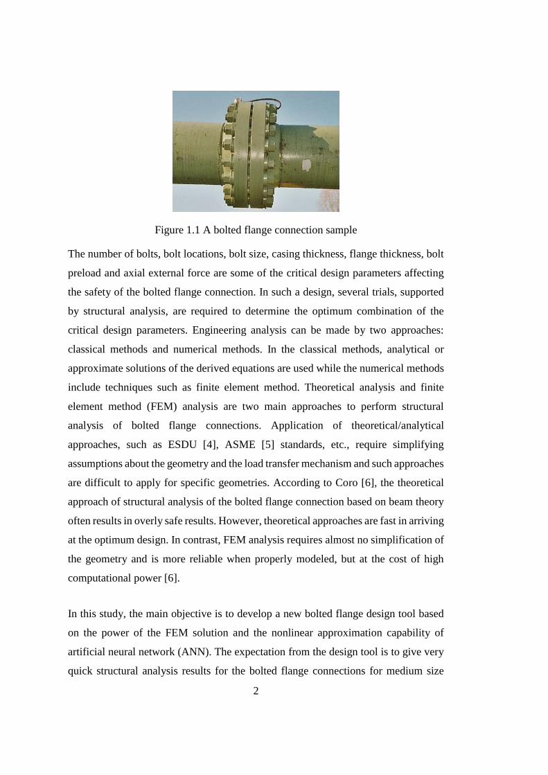
assembly [2]. Figure 1.1 presents a circular bolted flange connection. In bolted flange

connections, which are commonly utilized in aircraft engine designs, it is important

to achieve structural integrity and also to minimize the weight. The forces and

moments induced in an aircraft engine are transferred to other parts of the structure

through the bolted flange connections. On the other hand, an overly safe bolted flange

connection design leads to a heavier and less efficient aircraft engine. Since bolted

flange connections have a direct impact on the safety of the design [3] by serving as

load transfer mechanisms, structural analysis of the bolted flange connection should

be carried out with high attention in the detailed design stage. It takes hours or even

days to complete the analysis iterations as the number of degrees of freedom and the

nonlinearity level increase in the finite element analysis of the bolted flange

connection due to the contact definitions. Therefore, the standard finite element

analysis exercise causes to slow down the design process considerably. The need for

a bolted flange connection design tool that can reduce the engine weight in small

amount of computational time by generating quick, accurate analysis results is in a

way inevitable.

2

Figure 1.1 A bolted flange connection sample

The number of bolts, bolt locations, bolt size, casing thickness, flange thickness, bolt

preload and axial external force are some of the critical design parameters affecting

the safety of the bolted flange connection. In such a design, several trials, supported

by structural analysis, are required to determine the optimum combination of the

critical design parameters. Engineering analysis can be made by two approaches:

classical methods and numerical methods. In the classical methods, analytical or

approximate solutions of the derived equations are used while the numerical methods

include techniques such as finite element method. Theoretical analysis and finite

element method (FEM) analysis are two main approaches to perform structural

analysis of bolted flange connections. Application of theoretical/analytical

approaches, such as ESDU [4], ASME [5] standards, etc., require simplifying

assumptions about the geometry and the load transfer mechanism and such approaches

are difficult to apply for specific geometries. According to Coro [6], the theoretical

approach of structural analysis of the bolted flange connection based on beam theory

often results in overly safe results. However, theoretical approaches are fast in arriving

at the optimum design. In contrast, FEM analysis requires almost no simplification of

the geometry and is more reliable when properly modeled, but at the cost of high

computational power [6].

In this study, the main objective is to develop a new bolted flange design tool based

on the power of the FEM solution and the nonlinear approximation capability of

artificial neural network (ANN). The expectation from the design tool is to give very

quick structural analysis results for the bolted flange connections for medium size

3

aircraft engines without compromising the reliability. It should be noted that FEM

analysis requires longer model preparation and analysis times. For this purpose,

structural FE analysis in ANSYS Static Structural tool [7], parameters correlation

study in ANSYS DesignXplorer tool, and artificial neural network training in

MATLAB Neural Network tool [8] are used in combination to develop an ANN based

bolted flange design tool.

Linear behavior assumption in analysis is applicable to quite limited cases in real

world applications. On the contrary, the nature presents countless phenomena with

different types of nonlinearities. In the present study, several structural analysis should

be conducted including the nonlinear effects in order to simulate the deformation

mechanisms for the bolted flange connection. The nonlinear structural analysis needs

considerable amount of computational power since the process is iterative with

progressive modification as stated by Deng and Ghosn [9]. In a structural analysis,

one can mention three fundamental nonlinearity sources: material nonlinearity,

geometric nonlinearity, and boundary nonlinearity. The material nonlinearities can be

divided into three; time independent elastic-plastic behavior under load beyond yield

point, time dependent creep behavior under load with high temperature, and the

viscoelastic/viscoplastic behavior [10]. Large deflections or some critical deformation

shapes can cause geometric nonlinearities in solid structures [10]. Nonlinearities due

to boundary conditions are generally due to contact and friction [10].

Finite element problem solution can be achieved with the implementation of different

meshes on the geometry in consideration. One of the most critical factors affecting

the analysis results in FEM is the choice of element types to be used in the mesh

structure. In this study, 3D solid hexahedral elements are used because the geometry

is suitable to be filled with high quality hexahedral elements and meshing with

hexahedral elements give trustworthy results as it is explained later. A regular linear

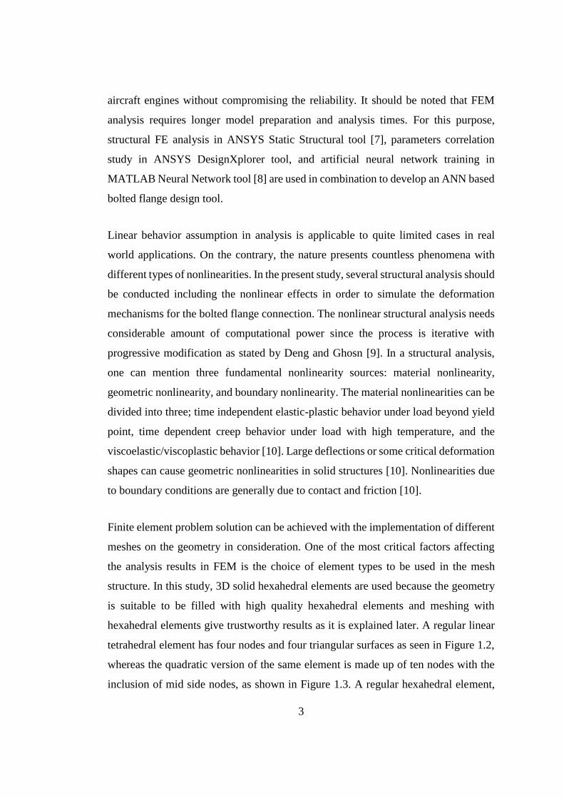
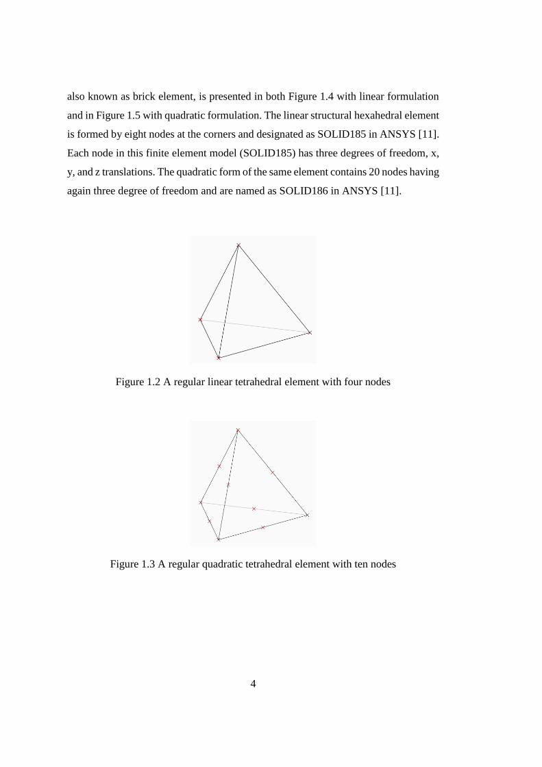
tetrahedral element has four nodes and four triangular surfaces as seen in Figure 1.2,

whereas the quadratic version of the same element is made up of ten nodes with the

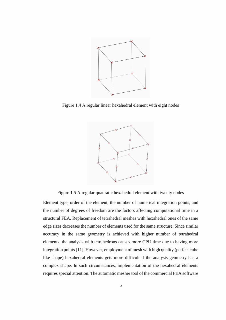
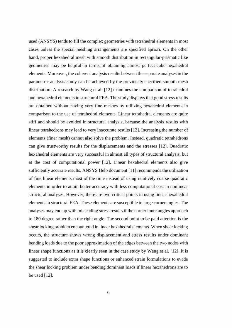
inclusion of mid side nodes, as shown in Figure 1.3. A regular hexahedral element,

4

also known as brick element, is presented in both Figure 1.4 with linear formulation

and in Figure 1.5 with quadratic formulation. The linear structural hexahedral element

is formed by eight nodes at the corners and designated as SOLID185 in ANSYS [11].

Each node in this finite element model (SOLID185) has three degrees of freedom, x,

y, and z translations. The quadratic form of the same element contains 20 nodes having

again three degree of freedom and are named as SOLID186 in ANSYS [11].

Figure 1.2 A regular linear tetrahedral element with four nodes

Figure 1.3 A regular quadratic tetrahedral element with ten nodes

5

Figure 1.4 A regular linear hexahedral element with eight nodes

Figure 1.5 A regular quadratic hexahedral element with twenty nodes

Element type, order of the element, the number of numerical integration points, and

the number of degrees of freedom are the factors affecting computational time in a

structural FEA. Replacement of tetrahedral meshes with hexahedral ones of the same

edge sizes decreases the number of elements used for the same structure. Since similar

accuracy in the same geometry is achieved with higher number of tetrahedral

elements, the analysis with tetrahedrons causes more CPU time due to having more

integration points [11]. However, employment of mesh with high quality (perfect cube

like shape) hexahedral elements gets more difficult if the analysis geometry has a

complex shape. In such circumstances, implementation of the hexahedral elements

requires special attention. The automatic mesher tool of the commercial FEA software

6

used (ANSYS) tends to fill the complex geometries with tetrahedral elements in most

cases unless the special meshing arrangements are specified apriori. On the other

hand, proper hexahedral mesh with smooth distribution in rectangular-prismatic like

geometries may be helpful in terms of obtaining almost perfect-cube hexahedral

elements. Moreover, the coherent analysis results between the separate analyses in the

parametric analysis study can be achieved by the previously specified smooth mesh

distribution. A research by Wang et al. [12] examines the comparison of tetrahedral

and hexahedral elements in structural FEA. The study displays that good stress results

are obtained without having very fine meshes by utilizing hexahedral elements in

comparison to the use of tetrahedral elements. Linear tetrahedral elements are quite

stiff and should be avoided in structural analysis, because the analysis results with

linear tetrahedrons may lead to very inaccurate results [12]. Increasing the number of

elements (finer mesh) cannot also solve the problem. Instead, quadratic tetrahedrons

can give trustworthy results for the displacements and the stresses [12]. Quadratic

hexahedral elements are very successful in almost all types of structural analysis, but

at the cost of computational power [12]. Linear hexahedral elements also give

sufficiently accurate results. ANSYS Help document [11] recommends the utilization

of fine linear elements most of the time instead of using relatively coarse quadratic

elements in order to attain better accuracy with less computational cost in nonlinear

structural analyses. However, there are two critical points in using linear hexahedral

elements in structural FEA. These elements are susceptible to large corner angles. The

analyses may end up with misleading stress results if the corner inner angles approach

to 180 degree rather than the right angle. The second point to be paid attention is the

shear locking problem encountered in linear hexahedral elements. When shear locking

occurs, the structure shows wrong displacement and stress results under dominant

bending loads due to the poor approximation of the edges between the two nodes with

linear shape functions as it is clearly seen in the case study by Wang et al. [12]. It is

suggested to include extra shape functions or enhanced strain formulations to evade

the shear locking problem under bending dominant loads if linear hexahedrons are to

be used [12].

7

The utilization of 3D finite elements in comparison to lower dimensions such as 1D

or 2D, the increase in the degrees of freedom, and the higher order of elements in FEM

result in complex equations in formation of element matrices during FEM solutions.

Moreover, mapping operation and inversion of Jacobian matrix are the other sources

increasing the complexity levels. Solving these equations by algebraic manipulations

is almost impossible. Therefore, numerical integration techniques are used to evaluate

equations in which the integrals are calculated by summation [13]. The numerical

integration is also known as “quadrature”. Gauss integration (Gauss quadrature) is the

most often used method in creation of element matrices by defining sampling points

and assigning weights to approximate integrals [14]. The number of sampling points

in Gauss quadrature determines the capability of approximating the order of integral.

In order to give accurate results for higher order integral, the numerical integration

points should be increased. If the number of integration points is sufficient to

approximate the higher order terms in stiffness equations of elements, it is called “full

integration”. On the other hand, if less integration points are used, the higher order

terms are excluded and this numerical integration is known as “reduced integration”.

However, the increase in the number of integration points does not change the

accuracy level after a certain point for a specific order of integrand. In ANSYS

Workbench, linear hexahedral elements with eight nodes use eight-point Gauss

integration rule in full integration [11]. On the other hand, quadratic hexahedral

elements formed by twenty nodes utilize fourteen-node Gauss integration rule in full

integration [11]. The increase of the number of integration points in an element causes

the increase of computational time in analysis. Utilization of full integration can cause

shear locking problem with over stiff elements and takes longer time in comparison

with reduced integration. On the other hand, reduced integration eliminates locking

problem and gives solution in less amount of time. However, reduced integration can

cause hourglass mode problem and the accuracy should be checked in this case.

Finite element analysis of multiple parts in the form of assemblies involves the

utilization of contacts. The knowledge about the contact formulation is valuable in

order to model the interaction between the contacting parts in a realistic way.

8

According to Cook et al. [15], the abrupt stiffness changes and the contact area

variations are the sources of nonlinearity in the problems with contacts. If the contact

stiffness is too low, overclosure (intersection) between two parts may occur. On the

other hand, too stiff contact causes probable convergence failures [15]. Contact

algorithms utilize special “contact elements” with special functions for detecting

contacts, preventing-limiting the penetration, and controlling the contact stiffness

[15]. The contact algorithms work on the principles of the slave nodes located on the

contacting surface of one part and the master nodes located on the other part. As stated

by the report [16]], checking the position of the slave nodes and detecting the

penetration of the master surface are the steps to explore the contact. Subsequently,

the slave nodes are relocated by pushing them back with respect to the master surface

[16]]. The critical parameters of the contact including the contact point, the

penetration level, and the pushback direction are controlled by the contact algorithms.

In most cases, the solution requires iterative approximations. The selection of the

master and slave surfaces is crucial in the solution process. If contacting surfaces are

made up of the same material, then the surface with coarser mesh should be chosen as

the master in order to prevent the undetected penetrations [16]]. Contact formulations

are derived by imposing constraint equations on the finite element solution via

minimization of potential energy. The commercial FEA software ANSYS [11] offers

four different contact formulations, pure penalty, normal Lagrange, multipoint

constraint, and augmented Lagrange. Multipoint constraint algorithm is applicable for

the cases with “no separation” or “bonded” contact types to tie surfaces with each

other [11]. In this study, there are no such type contacts used. The accuracy of penalty

(pure penalty) algorithm depends on the correct selection of the penalty term, µ, which

is also known as the contact stiffness. In this method, as the value of µ goes to infinity,

the algorithm satisfies the contact conditions exactly [17]. However, since such a

value cannot be stored in the solution matrices of the FEA, a finite value of penalty

term has to be selected. Thus, penalty algorithm is an approximate solution [17].

Although selecting large penalty values increases the solution accuracy, it also causes

numerically ill-conditioned problem such that the output error is highly sensitive to

the input error. On the other hand, penalty algorithm is easy to implement in problems

9

by only modifying the stiffness terms, and it also exhibits good convergence property

[11, 17]. In normal Lagrange algorithm, the Lagrange multiplier method is used, in

which the multiplier, λ, is also known as the contact force [11]. The negative aspect

of this method is the increase in the dimension of the solution matrix. Another

disadvantage is the fact that the solution matrix comprises zero-diagonal element(s)

so special technique is necessary to reorder and solve the equations. The main

advantage of this method is the ability of satisfying the exact contact conditions [17].

In the augmented Lagrange algorithm, the negative aspects of the penalty and the

Lagrange methods are aimed to be resolved. Consequently, augmented Lagrange

method is formulated by employing both the penalty term µ and the multiplier term λ

in order to reduce the high dependency on µ in the penalty method and discard the

increase of the solution matrix dimension as in the case of Lagrange multiplier method

[17]. In this method, an infinite µ is not required and λ can be controlled within the

desired tolerance [17]. In other words, the formulation is less sensitive to the correct

selection of µ in contrast to the penalty method. In this respect, the accuracy of the

nodal displacements is also controlled. The disadvantage of the augmented Lagrange

method is the necessity of iterative solution [17]. In this study, the contact algorithm

is augmented-Lagrange method with the default coefficients controlled by ANSYS.

Parametric finite element (FE) analysis is a common method utilized in design

practice of critical structural elements to obtain reliable design. Parametric study may

require hundreds or thousands of FE analyses depending on how crucial the design is

and how many input and output parameters exist to optimize the design. The

completion of thousands of FE analyses takes significant amount of time for limited

computational resources. Furthermore, all of the input parameters do not have the

same effect on the selected output parameters (results) in a parametric study. One

parameter may influence a specific output drastically whereas another one may hardly

change the same output. Therefore, in the present study, sensitivity study on the effect

of output on input parameters is carried out by utilizing parameters correlation study

in ANSYS. Parameters correlation study works on the basis of deterministic model

[11]. In contrast to the probabilistic models, no randomness is allowed in the

10

deterministic approach and one always gets the same output for a specific input.

Therefore, parameters correlation study can present accurate results depending on the

quantity and quality of the input. It is assessed that Spearman correlation is better in

identifying non-linear, monotonic relationships such as bolted flange connections

[11]. The principles of Spearman correlation will be explained in detail in the

corresponding section.

The artificial neural network is a group of computational cells, called as neurons, in

which each neuron has connections with all of the neurons located in the previous and

next layers with different weights defined in the training [18]. ANN is an effective

tool in approximating the non-linear relationships and the principles about ANN

methodology will be discussed further in corresponding section. In the study by

Muliana et al. [18], FE load displacement curves are generated with the help of ANN

where they observed that the trained ANN model is successful in predicting the

behavior of non-linear material property. Muliana et al. [18] also compared the

performance of ANN approximation with separate FEM analysis results to verify the

ANN performance. The study conducted by Muliana et al. proves the applicability

ANN approximation over non-linear finite element analysis.

One of the essential reference source in the field of bolted flange connection is

prepared by The Institution of Mechanical Engineers and established by ESDU [4].

This source discusses the problem of bolted flange under axial force by assuming the

structure as a beam. The methodology starts with idealizing the bolted flange

connection as an assembly of parallel springs formed by flange group and bolt group

as explained by Shigley in more detail [19]. By evaluating the material properties and

geometrical dimensions, the equivalent stiffnesses of both groups are calculated. Next,

external load is considered whether separation occurs under bolt head. According to

the result, prying effect is included or not in calculation of the corresponding bolt and

flange loads [4].

11

ASME Boiler and Pressure Vessel Code Section VIII [5] is a solid ground in the

literature with a very detailed theoretical approach to bolted flange connections. The

code considers the flange design with several aspects and presents design suggestions

and theoretical calculation methods and focuses especially on the complex flange

structures with several types generally containing gasket with internal pressure.

European standard on the flange calculation, EN 13445, considers ASME Code as a

basis as stated by Schaaf, et al. in an ASME conference proceeding [20].

Coro [6], describes a new flange design methodology based on finite element analysis.

Coro states that the finite element approach increases the level of precision in the

analysis of flange joint when compared to the theoretical solutions dependent on the

classical beam theory. The flange-design tool is mentioned to be a commercial product

that can analyze different flange geometries with different loading cases in a

parametric way. Although the author claims that flange-designer tool conducts

structural analysis based on FEM, the article hardly explains the working principles

or performance statistics. It should be noted that developed bolted flange tool

explained in the study by Coro [6] is claimed to give accurate results in comparison

with commercial FEA solution. The idea of utilizing FEM solution in a parametric

methodology

Azim [21] carried out an analytical investigation on bolt tension of the bolted flange

connection exposed to bending moments. The author examines the effects of

parameters such as flange thickness, width of the flange and the number of bolts on

the bolt tension by considering both the classical beam theory and FEM. Azim [21]

concludes that the theoretical approach has a limited applicability for real cases and

the error in the theoretical analysis increases as the input geometry differs from the

standard condition. In other words, the theoretical approach in that study gives reliable

results only for a limited range of the input. Therefore, it can be concluded that the

theoretical analysis of bolted flange connection cannot be trusted all the time. Instead,

analysis by FEM should be preferred in the analysis of such a critical structure.

12

In this study, a methodology has been developed for the iterative design and analysis

of the bolted flange connection by utilizing artificial neural network approximation

(ANN) of the database formed with thirteen thousand five hundred non-linear FE

analyses involving contact under axial external load. “Function fitting” approach is

used to train and then predict the complex, non-linear input output-behavior of the

bolted flange connections using finite element analysis [22]. The main motivation of

the study is to develop an ANN based bolted flange design tool for medium sized

aircraft engines. The bolted flange design tool will be used in the preliminary design

stage to assess the structural integrity of the bolted flanges very fast for various

choices of the design parameters. Thus, long model preparation and analysis

requirement of direct non-linear finite element based analysis will be eliminated and

substantial reduction in design cycle time will be achieved. The flange design tool

will also be used as the fast solver, which will replace the finite element solver, in

conjunction with an optimizer to achieve weight reduction in the flange. Weight

saving in any structural component of aircraft is one of the main goals in the design

of aircraft.

13

CHAPTER 2

SCOPE OF THE THESIS

In this study, a methodology has been developed for the iterative design and analysis

of bolted flange connections by utilizing artificial neural network approximation

(ANN) of FEM analysis database formed with 13500 fine-meshed, non-linear

structural analyses involving contact under axial external load.

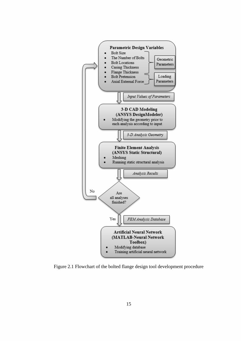
Flowchart of the developed bolted flange design tool is presented in Figure 2.1. In

chapter 3, determination of the analysis geometry and the input parameters is

explained. There are seven input parameters, five of which are geometric parameters

and the remaining two parameters are for load input. The analysis geometry is

modeled in ANSYS DesignModeler [7] as 3-D computer aided drawing (CAD) file

by considering the subsequent parametric study. In the next step, the analysis model

is prepared in ANSYS-Static Structural module. In order to investigate the effects of

input parameters on the output, parameters correlation study is conducted in ANSYS

DesignXplorer tool [7] as described in chapter 4. According to the result of parameters

correlation study, the input value intervals of the parameters within the upper and

lower ranges of the parameters are determined. By running successive static structural

FEM analysis, a database of 13500 analyses is formed by combining all the selected

parametric design variables with each other. Subsequently, chapter 5 presents the

artificial neural network training process with the finalized FEM analysis database to

obtain a continuous solution domain within the upper and lower limits of the

parameters.

In chapter 6 of the thesis, the developed bolted flange connection design tool is tested

against different test cases to verify the performance of the design tool. The first test

set is formed by ten test points which are exactly located on the initial training points

of the design tool. In the second test set, there are ten test points which are not same

14

as the parameter design points, but selected inside the training points within the upper

and lower limits of the parameters. The final test set consists of ten instances located

outside the training limits. Furthermore, the performance of the developed tool is

compared with the analytical approach of ESDU [4] for the same example problem.

In the last chapter, whole study is summarized and the outcome is evaluated as well

as stating the future work possibilities. Both case studies for testing shows that the

developed bolted flange design can be used as a fast solver with very high accuracy

within the training limits of the input parameters.

15

Figure 2.1 Flowchart of the bolted flange design tool development procedure

17

CHAPTER 3

FINITE ELEMENT ANALYSIS OF BOLTED FLANGE

CONNECTION

Running structural finite element analysis (FEA) is a task with a trade-off between

accurate results and computational power. Geometric and material non-linearities,

existence of contacts between different parts, mesh size are some of the factors

draining the computational sources.

In this study, finite element analysis (FEA) of bolted flange connection is carried out

in an automated parametric study. To conduct thirteen thousand five hundred analyses

in a parametric set with five geometric and two loading input parameters, the analysis

model must be so arranged that parametric meshing operation should not fail to mesh

the analysis geometry. Otherwise, the software cannot create the expected finite

elements as defined by the initial settings so the analysis cannot converge to any result.

The failed analyses cause data point losses, which are required for artificial neural

network training.

ANSYS Workbench [7] is the finite element analysis software utilized in all the static

structural analyses. DesignModeler toolbox [7] is employed for creation and

modification of the analysis geometry.

The finite element analysis model is prepared by following certain steps. The 3D

analysis assembly is modeled according to defined values of the geometric variables.

The selected materials are assigned to corresponding parts in assembly. The contacts

are defined between the parts of the analysis in Static Structural interface [7]. Meshing

operation takes place according to the previously defined mesh method and sizing

settings. After all required static structural analysis settings such as the number of

solution steps or nonlinear solution options are specified, load and boundary

18

conditions are imposed on the analysis model. In the last step, the types of output

results expected form the analysis are settled. Once all these steps are finalized, one

can immediately run the analysis if it is single analysis. On the other hand, if the case

is a parametric analysis study, the solution process of multiple analyses (design points)

has to be commenced after the definition of the input parameter values for the desired

number of design points.

3.1 Analysis Geometry and Meshing

In this study, the area of interest is scoped out a medium scale bolted flange connection

of an aircraft engine. The engine model with the nominal geometrical dimensions, the

loading conditions, and the bolt pretension, have been previously specified prior to

this study [23]. In the present study, the defined circular bolted flange connection is

exposed to an axial external force. It is intended to optimize the modeling of the

analysis geometry, meshing operation, and defining analysis details in order to run

successfully the analyses of parametric sets in an automated way. The details are

expressed in the corresponding sections.

3.1.1 Bolted Flange Connection Assembly

In line with the specified analysis model, a fully circular bolted flange connection

structure is formed by two symmetrical flange extensions with nominal twenty four

equally spaced bolt and nut pairs, and two identical washers for each bolt-nut pair

(one being located between the bolt head and the flange-1, and the latter between the

nut and the flange-2). The flange structure type is designated as inverted T-shape [6]

in which the flanges are extended radially outward from casing. Figure 3.1 shows the

complete geometry of the bolted flange connection to be analyzed in this study.

Because the bolted flange connection geometry is circular with equally spaced bolt-

nut pairs, the structure can be sliced into twenty four (equal to the number of bolts)

identical sectors about the internal axis (z-axis in this study).

19

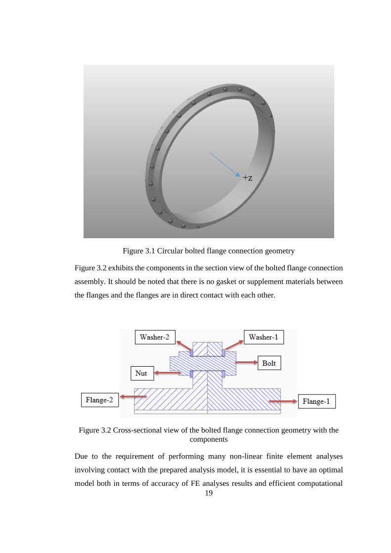
Figure 3.1 Circular bolted flange connection geometry

Figure 3.2 exhibits the components in the section view of the bolted flange connection

assembly. It should be noted that there is no gasket or supplement materials between

the flanges and the flanges are in direct contact with each other.

Figure 3.2 Cross-sectional view of the bolted flange connection geometry with the

components

Due to the requirement of performing many non-linear finite element analyses

involving contact with the prepared analysis model, it is essential to have an optimal

model both in terms of accuracy of FE analyses results and efficient computational

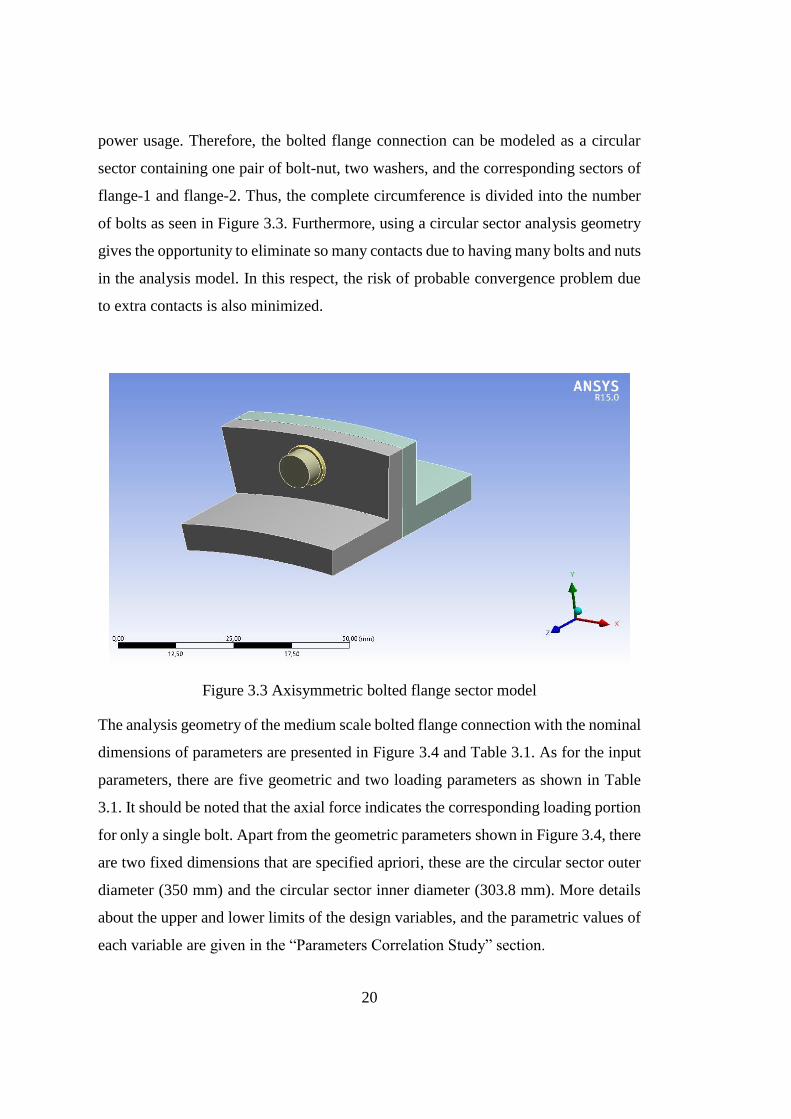
20

power usage. Therefore, the bolted flange connection can be modeled as a circular

sector containing one pair of bolt-nut, two washers, and the corresponding sectors of

flange-1 and flange-2. Thus, the complete circumference is divided into the number

of bolts as seen in Figure 3.3. Furthermore, using a circular sector analysis geometry

gives the opportunity to eliminate so many contacts due to having many bolts and nuts

in the analysis model. In this respect, the risk of probable convergence problem due

to extra contacts is also minimized.

Figure 3.3 Axisymmetric bolted flange sector model

The analysis geometry of the medium scale bolted flange connection with the nominal

dimensions of parameters are presented in Figure 3.4 and Table 3.1. As for the input

parameters, there are five geometric and two loading parameters as shown in Table

3.1. It should be noted that the axial force indicates the corresponding loading portion

for only a single bolt. Apart from the geometric parameters shown in Figure 3.4, there

are two fixed dimensions that are specified apriori, these are the circular sector outer

diameter (350 mm) and the circular sector inner diameter (303.8 mm). More details

about the upper and lower limits of the design variables, and the parametric values of

each variable are given in the “Parameters Correlation Study” section.

21

Figure 3.4 The circular sector analysis model with the geometric parameters

22

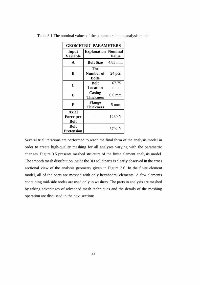
Table 3.1 The nominal values of the parameters in the analysis model

GEOMETRIC PARAMETERS

Input

Variable

Explanation Nominal

Value

A Bolt Size 4.83 mm

B

The

Number of

Bolts

24 pcs

C Bolt

Location

167.75

mm

D Casing

Thickness 6.6 mm

E Flange

Thickness 5 mm

Axial

Force per

Bolt

- 1280 N

Bolt

Pretension - 5702 N

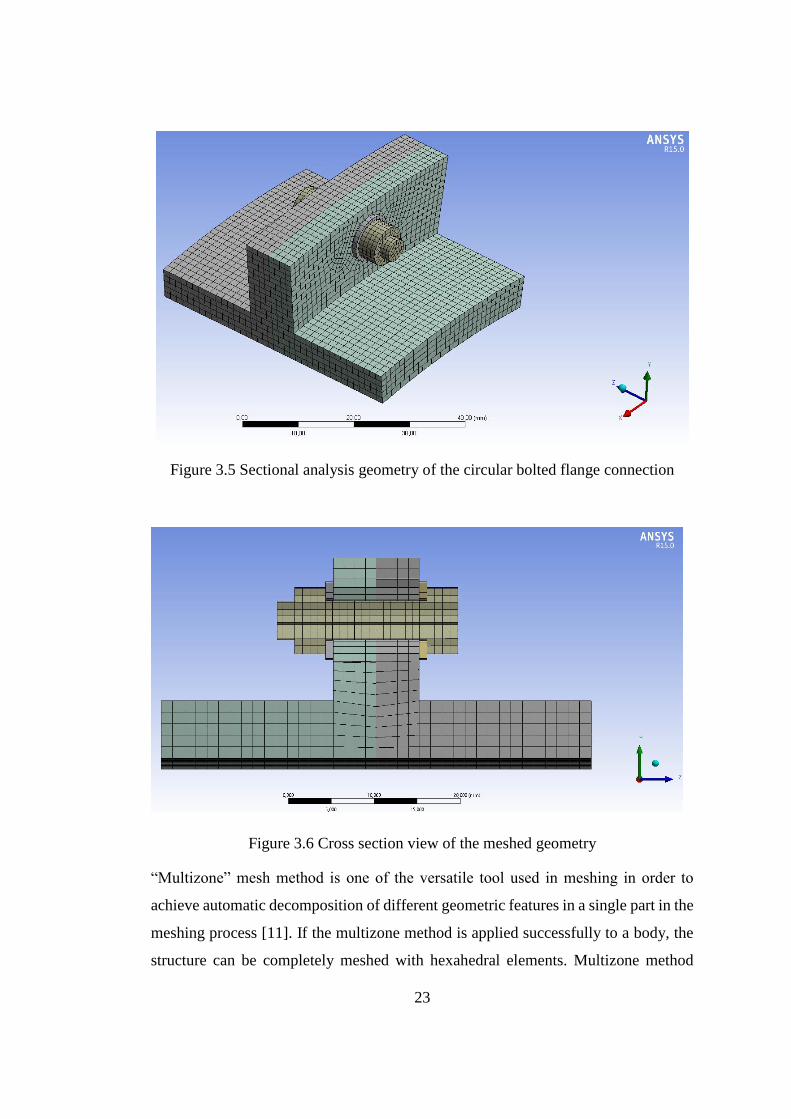
Several trial iterations are performed to reach the final form of the analysis model in

order to create high-quality meshing for all analyses varying with the parametric

changes. Figure 3.5 presents meshed structure of the finite element analysis model.

The smooth mesh distribution inside the 3D solid parts is clearly observed in the cross

sectional view of the analysis geometry given in Figure 3.6. In the finite element

model, all of the parts are meshed with only hexahedral elements. A few elements

containing mid-side nodes are used only in washers. The parts in analysis are meshed

by taking advantages of advanced mesh techniques and the details of the meshing

operation are discussed in the next sections.

23

Figure 3.5 Sectional analysis geometry of the circular bolted flange connection

Figure 3.6 Cross section view of the meshed geometry

“Multizone” mesh method is one of the versatile tool used in meshing in order to

achieve automatic decomposition of different geometric features in a single part in the

meshing process [11]. If the multizone method is applied successfully to a body, the

structure can be completely meshed with hexahedral elements. Multizone method

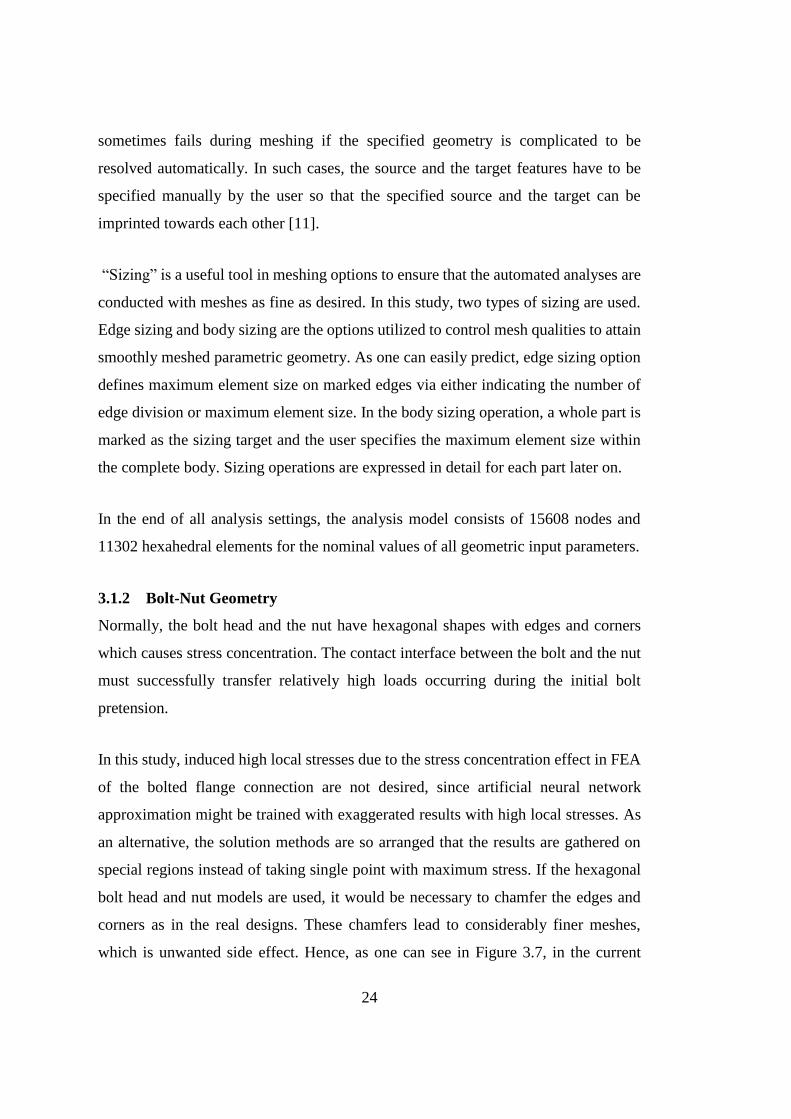
24

sometimes fails during meshing if the specified geometry is complicated to be

resolved automatically. In such cases, the source and the target features have to be

specified manually by the user so that the specified source and the target can be

imprinted towards each other [11].

“Sizing” is a useful tool in meshing options to ensure that the automated analyses are

conducted with meshes as fine as desired. In this study, two types of sizing are used.

Edge sizing and body sizing are the options utilized to control mesh qualities to attain

smoothly meshed parametric geometry. As one can easily predict, edge sizing option

defines maximum element size on marked edges via either indicating the number of

edge division or maximum element size. In the body sizing operation, a whole part is

marked as the sizing target and the user specifies the maximum element size within

the complete body. Sizing operations are expressed in detail for each part later on.

In the end of all analysis settings, the analysis model consists of 15608 nodes and

11302 hexahedral elements for the nominal values of all geometric input parameters.

3.1.2 Bolt-Nut Geometry

Normally, the bolt head and the nut have hexagonal shapes with edges and corners

which causes stress concentration. The contact interface between the bolt and the nut

must successfully transfer relatively high loads occurring during the initial bolt

pretension.

In this study, induced high local stresses due to the stress concentration effect in FEA

of the bolted flange connection are not desired, since artificial neural network

approximation might be trained with exaggerated results with high local stresses. As

an alternative, the solution methods are so arranged that the results are gathered on

special regions instead of taking single point with maximum stress. If the hexagonal

bolt head and nut models are used, it would be necessary to chamfer the edges and

corners as in the real designs. These chamfers lead to considerably finer meshes,

which is unwanted side effect. Hence, as one can see in Figure 3.7, in the current

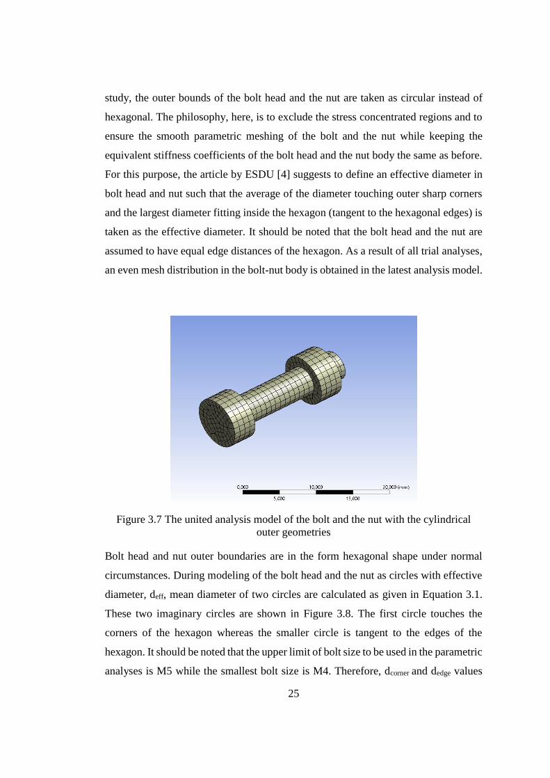
25

study, the outer bounds of the bolt head and the nut are taken as circular instead of

hexagonal. The philosophy, here, is to exclude the stress concentrated regions and to

ensure the smooth parametric meshing of the bolt and the nut while keeping the

equivalent stiffness coefficients of the bolt head and the nut body the same as before.

For this purpose, the article by ESDU [4] suggests to define an effective diameter in

bolt head and nut such that the average of the diameter touching outer sharp corners

and the largest diameter fitting inside the hexagon (tangent to the hexagonal edges) is

taken as the effective diameter. It should be noted that the bolt head and the nut are

assumed to have equal edge distances of the hexagon. As a result of all trial analyses,

an even mesh distribution in the bolt-nut body is obtained in the latest analysis model.

Figure 3.7 The united analysis model of the bolt and the nut with the cylindrical

outer geometries

Bolt head and nut outer boundaries are in the form hexagonal shape under normal

circumstances. During modeling of the bolt head and the nut as circles with effective

diameter, deff, mean diameter of two circles are calculated as given in Equation 3.1.

These two imaginary circles are shown in Figure 3.8. The first circle touches the

corners of the hexagon whereas the smaller circle is tangent to the edges of the

hexagon. It should be noted that the upper limit of bolt size to be used in the parametric

analyses is M5 while the smallest bolt size is M4. Therefore, dcorner and dedge values

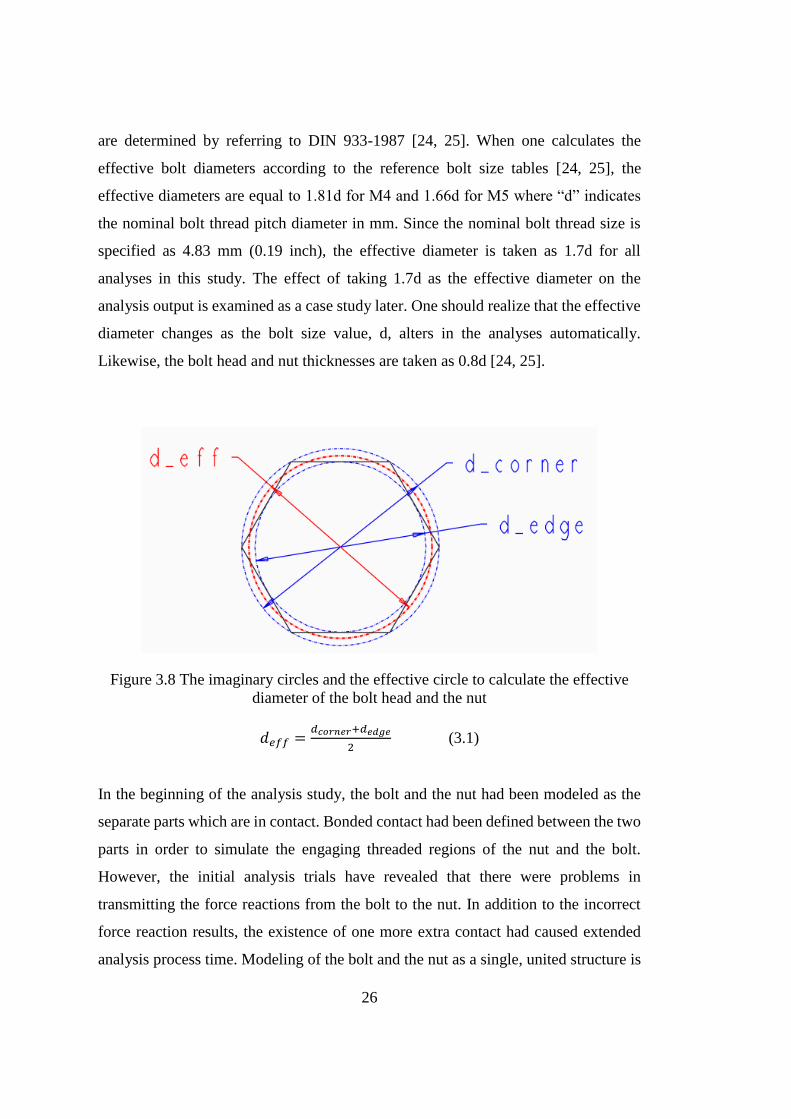
26

are determined by referring to DIN 933-1987 [24, 25]. When one calculates the

effective bolt diameters according to the reference bolt size tables [24, 25], the

effective diameters are equal to 1.81d for M4 and 1.66d for M5 where “d” indicates

the nominal bolt thread pitch diameter in mm. Since the nominal bolt thread size is

specified as 4.83 mm (0.19 inch), the effective diameter is taken as 1.7d for all

analyses in this study. The effect of taking 1.7d as the effective diameter on the

analysis output is examined as a case study later. One should realize that the effective

diameter changes as the bolt size value, d, alters in the analyses automatically.

Likewise, the bolt head and nut thicknesses are taken as 0.8d [24, 25].

Figure 3.8 The imaginary circles and the effective circle to calculate the effective

diameter of the bolt head and the nut

𝑑𝑒𝑓𝑓 =𝑑𝑐𝑜𝑟𝑛𝑒𝑟+𝑑𝑒𝑑𝑔𝑒

2 (3.1)

In the beginning of the analysis study, the bolt and the nut had been modeled as the

separate parts which are in contact. Bonded contact had been defined between the two

parts in order to simulate the engaging threaded regions of the nut and the bolt.

However, the initial analysis trials have revealed that there were problems in

transmitting the force reactions from the bolt to the nut. In addition to the incorrect

force reaction results, the existence of one more extra contact had caused extended

analysis process time. Modeling of the bolt and the nut as a single, united structure is

27

seen to give the correct reaction forces and excludes the need for the bonded contact

between the inner surface of the nut and the threaded section of the bolt. Both the bolt

and the nut are made up of same material in this study. Hence, the united, single body

modeling of the bolt and nut is a realistic engineering approach. The united bolt-nut

model is given in Figure 3.7 as mentioned before.

To ensure the proper meshing of the bolt-nut body during the automated parametric

analyses (bolt diameter is one of the geometric parameters), multizone mesh method

is implemented in the bolt-nut body. As seen in Figure 3.7, the inner cylinder (bolt

thread and shank portions together) is decomposed from the imaginary outer hollow

cylinders of the bolt head and the nut. As a result, high quality hexagonal meshes are

generated at a rate of one hundred percent without having any tetrahedral or triangular

prism elements as desired.

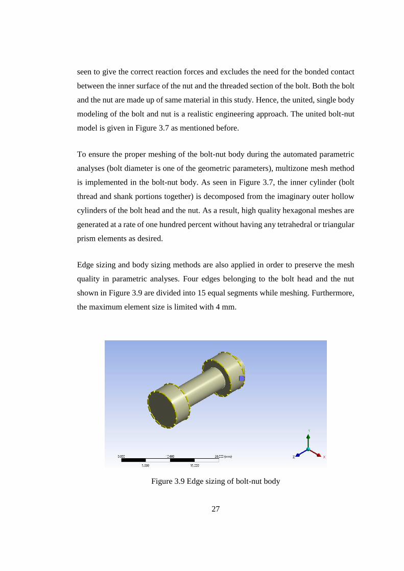
Edge sizing and body sizing methods are also applied in order to preserve the mesh

quality in parametric analyses. Four edges belonging to the bolt head and the nut

shown in Figure 3.9 are divided into 15 equal segments while meshing. Furthermore,

the maximum element size is limited with 4 mm.

Figure 3.9 Edge sizing of bolt-nut body

28

3.1.3 Flange Geometry

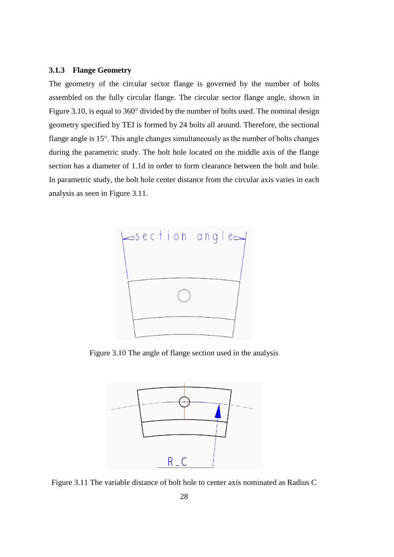
The geometry of the circular sector flange is governed by the number of bolts

assembled on the fully circular flange. The circular sector flange angle, shown in

Figure 3.10, is equal to 360° divided by the number of bolts used. The nominal design

geometry specified by TEI is formed by 24 bolts all around. Therefore, the sectional

flange angle is 15°. This angle changes simultaneously as the number of bolts changes

during the parametric study. The bolt hole located on the middle axis of the flange

section has a diameter of 1.1d in order to form clearance between the bolt and hole.

In parametric study, the bolt hole center distance from the circular axis varies in each

analysis as seen in Figure 3.11.

Figure 3.10 The angle of flange section used in the analysis

Figure 3.11 The variable distance of bolt hole to center axis nominated as Radius C

29

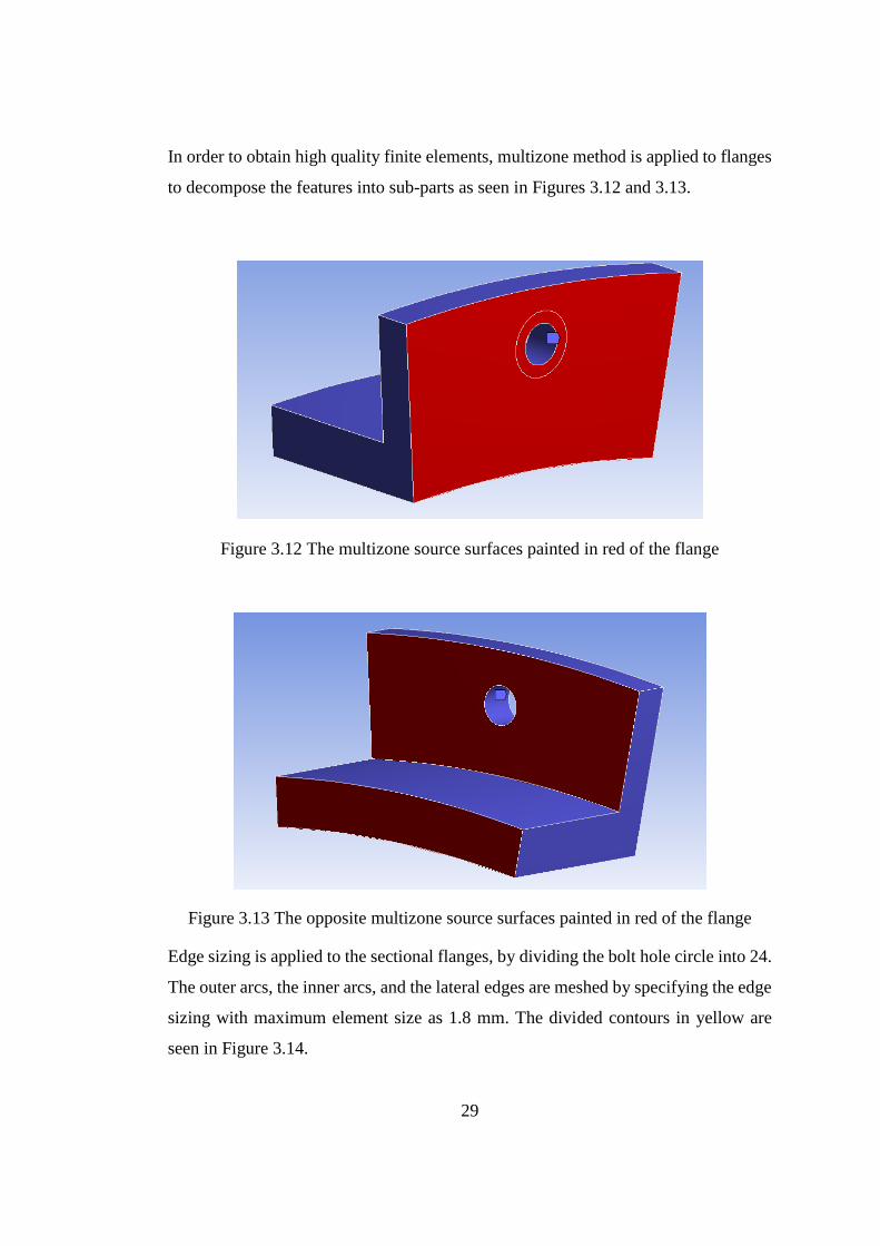
In order to obtain high quality finite elements, multizone method is applied to flanges

to decompose the features into sub-parts as seen in Figures 3.12 and 3.13.

Figure 3.12 The multizone source surfaces painted in red of the flange

Figure 3.13 The opposite multizone source surfaces painted in red of the flange

Edge sizing is applied to the sectional flanges, by dividing the bolt hole circle into 24.

The outer arcs, the inner arcs, and the lateral edges are meshed by specifying the edge

sizing with maximum element size as 1.8 mm. The divided contours in yellow are

seen in Figure 3.14.

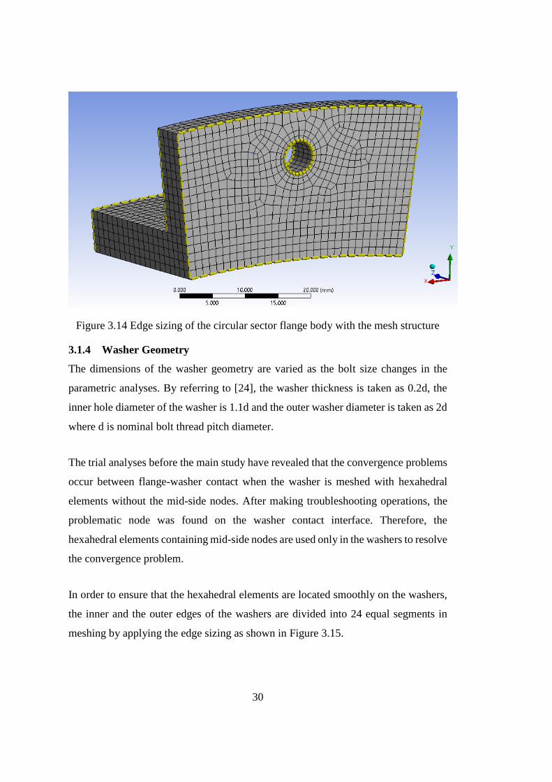
30

Figure 3.14 Edge sizing of the circular sector flange body with the mesh structure

3.1.4 Washer Geometry

The dimensions of the washer geometry are varied as the bolt size changes in the

parametric analyses. By referring to [24], the washer thickness is taken as 0.2d, the

inner hole diameter of the washer is 1.1d and the outer washer diameter is taken as 2d

where d is nominal bolt thread pitch diameter.

The trial analyses before the main study have revealed that the convergence problems

occur between flange-washer contact when the washer is meshed with hexahedral

elements without the mid-side nodes. After making troubleshooting operations, the

problematic node was found on the washer contact interface. Therefore, the

hexahedral elements containing mid-side nodes are used only in the washers to resolve

the convergence problem.

In order to ensure that the hexahedral elements are located smoothly on the washers,

the inner and the outer edges of the washers are divided into 24 equal segments in

meshing by applying the edge sizing as shown in Figure 3.15.

31

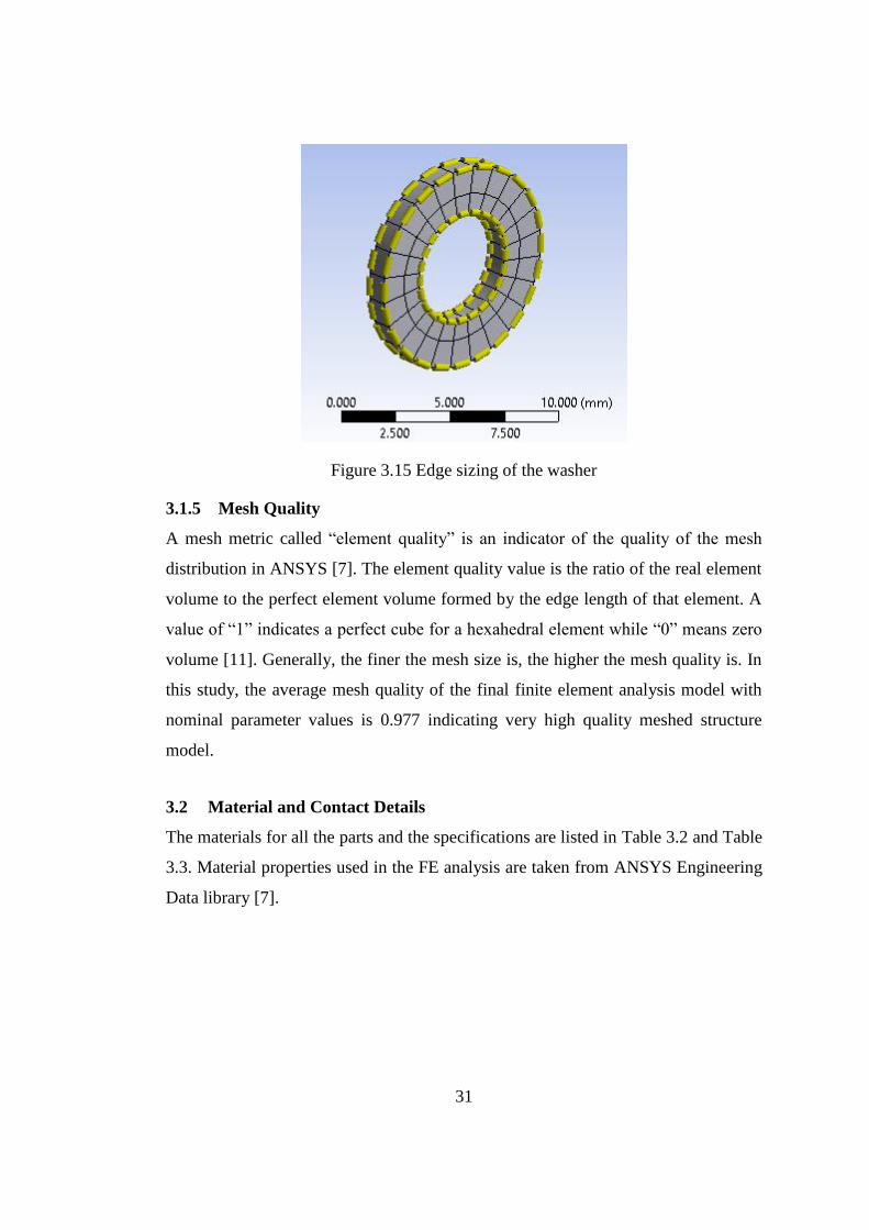
Figure 3.15 Edge sizing of the washer

3.1.5 Mesh Quality

A mesh metric called “element quality” is an indicator of the quality of the mesh

distribution in ANSYS [7]. The element quality value is the ratio of the real element

volume to the perfect element volume formed by the edge length of that element. A

value of “1” indicates a perfect cube for a hexahedral element while “0” means zero

volume [11]. Generally, the finer the mesh size is, the higher the mesh quality is. In

this study, the average mesh quality of the final finite element analysis model with

nominal parameter values is 0.977 indicating very high quality meshed structure

model.

3.2 Material and Contact Details

The materials for all the parts and the specifications are listed in Table 3.2 and Table

3.3. Material properties used in the FE analysis are taken from ANSYS Engineering

Data library [7].

32

Table 3.2 Material properties used in the analysis model [7]

MATERIAL PROPERTIES

Material Young's

Modulus

(E), GPa

Poisson's

Ratio (v)

Structural

Steel 200 0.3

Aluminum

Alloy 71 0.33

Table 3.3 Materials of the components in analysis model

MATERIALS OF THE PARTS

Flange-1 Aluminum Alloy

Flange-2 Aluminum Alloy

Bolt-Nut Body Structural Steel

Washer-1 Structural Steel

Washer-2 Structural Steel

In the analysis model, two contact types are used. The first type is the frictional contact

with the specific friction coefficient depending on the materials of the contact pairs.

In Figure 3.16, the contacts 1, 2, 3, 4, and 5 are of this type. The latter type is the

frictionless contact. In this contact type, the parts in contact act as frictionless supports

against each other. The frictionless contact is used between the bolt body, including

the threaded and the shank portions together, and the hole surfaces of the other parts

through which the bolt body passes. It should be noted that although there are no

permanent contacts between the bolt body and the other parts all the time since the

holes are slightly bigger than the bolt diameter, the frictionless contacts are used in

order to prevent probable interferences of the contact parts. All of the designated

contact pairs shown in Figure 3.16 are presented with the part names, contact types,

and the friction coefficients in Table 3.4.

33

Figure 3.16 Representations of the contacts on the cross-sectional bolted flange

connection view

Table 3.4 Contact details of the analysis model according to Figure 3.16

CONTACT DETAILS

Contact

No.

Contact

Part-1

Contact

Part-2

Contact

Type

Static Friction

Coefficient [26]

1 Flange-1 Flange-2 Frictional 1.20

2 Washer-1 Flange-1 Frictional 0.61

3 Flange-2 Washer-2 Frictional 0.61

4 Bolt-Nut Washer-1 Frictional 0.74

5 Washer-2 Bolt-Nut Frictional 0.74

6 Bolt-Nut Washer-1 Frictionless N/A

7 Bolt-Nut Flange-1 Frictionless N/A

8 Bolt-Nut Flange-2 Frictionless N/A

9 Bolt-Nut Washer-2 Frictionless N/A

All remaining settings related with the contacts such as penetration tolerance, contact

stiffness, etc. are taken as the default settings of ANSYS in program controlled mode

[7]. The contact formulation algorithm is Augmented Lagrange method while Gauss

integration point is used as the contact detection method. The penetration tolerance in

each contact is determined by the software.

3.3 Load and Boundary Conditions

The loading applied to flange-2 as the axial external force and the boundary conditions

of the model are seen in Figure 3.17. There is a fixed support, in which all degree of

freedoms are fixed, applied on the opposite surface on flange-1. The surface of flange-

34

2 in Figure 3.17, on which the force is applied, is fixed in radial and tangential

directions. The lateral surfaces designated with 1 and 2 in Figure 3.18 for both flange-

1 and flange-2 are constrained in the tangential direction. In flange-1 and flange-2, the

surfaces of 3 and 4 are free surfaces. The terms, ur, uθ beyond each surface in figures

indicate the boundary conditions of the related surfaces.

Figure 3.17 Load and boundary conditions; the fixed end on the right and the

external force applied on the left

Figure 3.18 Load and boundary conditions: the designated lateral surfaces of the

analysis geometry

3.4 Analysis Properties

The bolted flange connection loading in normal service conditions takes place in two

successive steps. Firstly, all of the bolts are tightened with the required amount of

torque to apply the bolt preload. Secondly, the loading conditions occur on the

connection once the service begins. Therefore, the finite element analysis of bolted

35

flange connection must be performed in two steps as well. In the first step, the bolt

pretension is applied and the axial external force is applied in the second step.

No thermal load or temperature changes have been previously specified in this study.

However, if there were such a need in analysis, the number of solution steps could be

increased from two to three or the thermal condition could be applied simultaneously

with axial external load in two steps.

The FEM software makes several analysis settings available for user in order to

control the analysis details. One of them is the auto time stepping option, which is a

beneficial tool especially for nonlinear analyses [11]. In this option for the sub-steps

of each step, “program controlled” mode has been selected in which the minimum

number of sub-steps is one whereas the maximum is ten sub-steps for the nonlinear

static structural analysis. In this mode, the software decides itself to divide the solution

step into sub-steps within the stated limits depending on the convergence of the

solution.

Initial analyses were performed including geometric nonlinearity, but the results

showed that the maximum deformation value is rather small in comparison to the

dimensions of the geometry. Hence, small deflection is assumed and the remaining

analyses are performed utilizing small deflection assumption.

The nonlinear finite element analysis setup is solved by Newton-Raphson solution

method as a default setting of the software.

3.5 Finite Element Solution of the Bolted Flange Connection

In order to evade getting misguiding results in the ANN training, finite element

analysis of the bolted flange connection is evaluated by means of the average stress in

a pre-defined contour in the flange instead of using the maximum stress values caused

by the singularities or the stress concentrations. As observed in the preparatory

analyses, high stress regions appear in the threaded and the shank portions for the bolt-

nut single body while high stress area is observed on the matching faces of the flanges

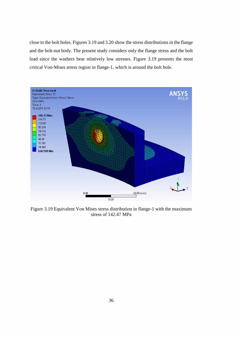
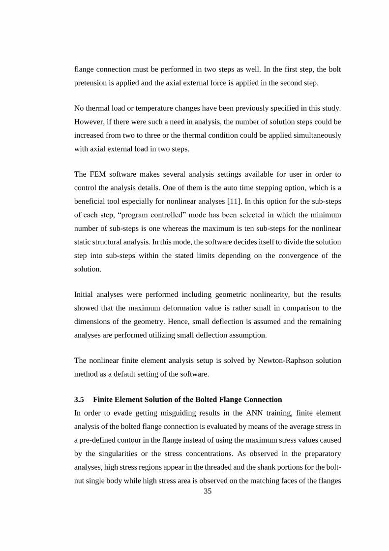
36

close to the bolt holes. Figures 3.19 and 3.20 show the stress distributions in the flange

and the bolt-nut body. The present study considers only the flange stress and the bolt

load since the washers bear relatively low stresses. Figure 3.19 presents the most

critical Von-Mises stress region in flange-1, which is around the bolt hole.

Figure 3.19 Equivalent Von Mises stress distribution in flange-1 with the maximum

stress of 142.47 MPa

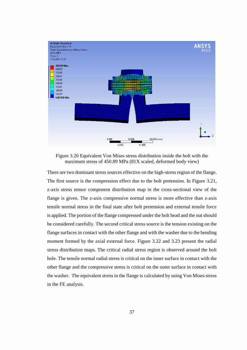
37

Figure 3.20 Equivalent Von Mises stress distribution inside the bolt with the

maximum stress of 450.89 MPa (81X scaled, deformed body view)

There are two dominant stress sources effective on the high-stress region of the flange.

The first source is the compression effect due to the bolt pretension. In Figure 3.21,

z-axis stress tensor component distribution map in the cross-sectional view of the

flange is given. The z-axis compressive normal stress is more effective than z-axis

tensile normal stress in the final state after bolt pretension and external tensile force

is applied. The portion of the flange compressed under the bolt head and the nut should

be considered carefully. The second critical stress source is the tension existing on the

flange surfaces in contact with the other flange and with the washer due to the bending

moment formed by the axial external force. Figure 3.22 and 3.23 present the radial

stress distribution maps. The critical radial stress region is observed around the bolt

hole. The tensile normal radial stress is critical on the inner surface in contact with the

other flange and the compressive stress is critical on the outer surface in contact with

the washer. The equivalent stress in the flange is calculated by using Von Mises stress

in the FE analysis.

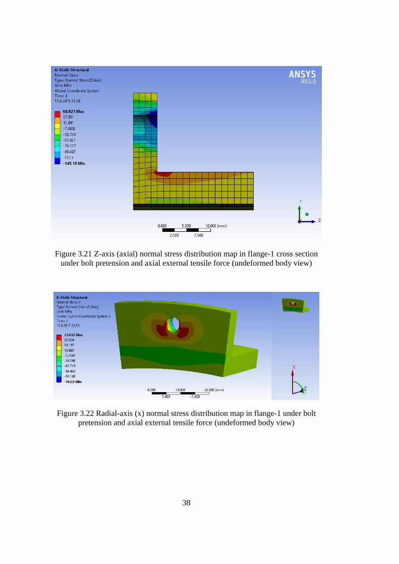
38

Figure 3.21 Z-axis (axial) normal stress distribution map in flange-1 cross section

under bolt pretension and axial external tensile force (undeformed body view)


pretension and axial external tensile force (undeformed body view)

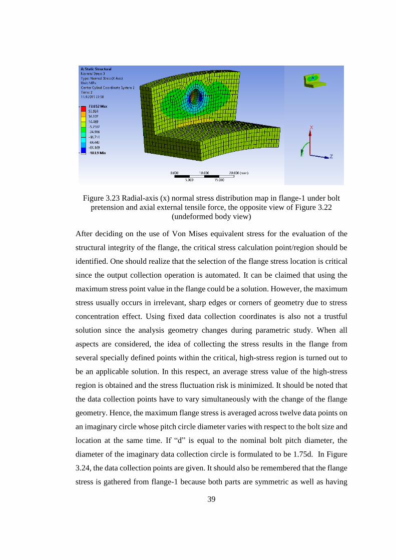
39


pretension and axial external tensile force, the opposite view of Figure 3.22

(undeformed body view)

After deciding on the use of Von Mises equivalent stress for the evaluation of the

structural integrity of the flange, the critical stress calculation point/region should be

identified. One should realize that the selection of the flange stress location is critical

since the output collection operation is automated. It can be claimed that using the

maximum stress point value in the flange could be a solution. However, the maximum

stress usually occurs in irrelevant, sharp edges or corners of geometry due to stress

concentration effect. Using fixed data collection coordinates is also not a trustful

solution since the analysis geometry changes during parametric study. When all

aspects are considered, the idea of collecting the stress results in the flange from

several specially defined points within the critical, high-stress region is turned out to

be an applicable solution. In this respect, an average stress value of the high-stress

region is obtained and the stress fluctuation risk is minimized. It should be noted that

the data collection points have to vary simultaneously with the change of the flange

geometry. Hence, the maximum flange stress is averaged across twelve data points on

an imaginary circle whose pitch circle diameter varies with respect to the bolt size and

location at the same time. If “d” is equal to the nominal bolt pitch diameter, the

diameter of the imaginary data collection circle is formulated to be 1.75d. In Figure

3.24, the data collection points are given. It should also be remembered that the flange

stress is gathered from flange-1 because both parts are symmetric as well as having

40

almost symmetrical loads and boundary conditions. The contact status between

flange-1 and flange-2 in the end of the analysis can be observed in Figure 3.25 in

which the dark orange and the light orange painted regions imply the contacting

surfaces of flange-1 and flange-2. Apparently, the smallest diameter inside the

sticking and sliding region is about 1.75d as seen in Figure 3.25. In theoretical solution

method, the flange stress is calculated by taking an effective diameter inside the

contact region, in which equal stress distribution is assumed inside the effective

diameter for an axial load [4]. On the other hand, as one can realize by considering

Figure 3.26, taking smaller stress collection circle causes the average stress results to

increase greatly. For those reasons, the stress data collection circle is selected to be

the one with the largest diameter, which is also inside the direct contact region.

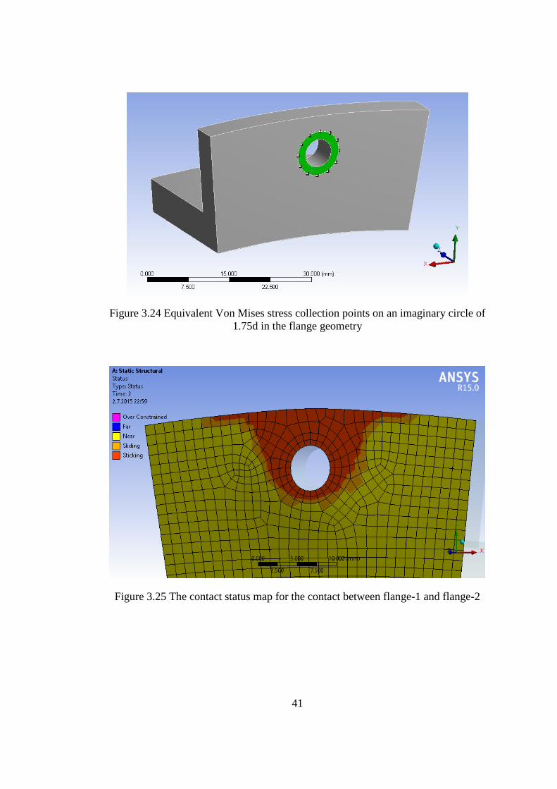
41

Figure 3.24 Equivalent Von Mises stress collection points on an imaginary circle of

1.75d in the flange geometry

Figure 3.25 The contact status map for the contact between flange-1 and flange-2

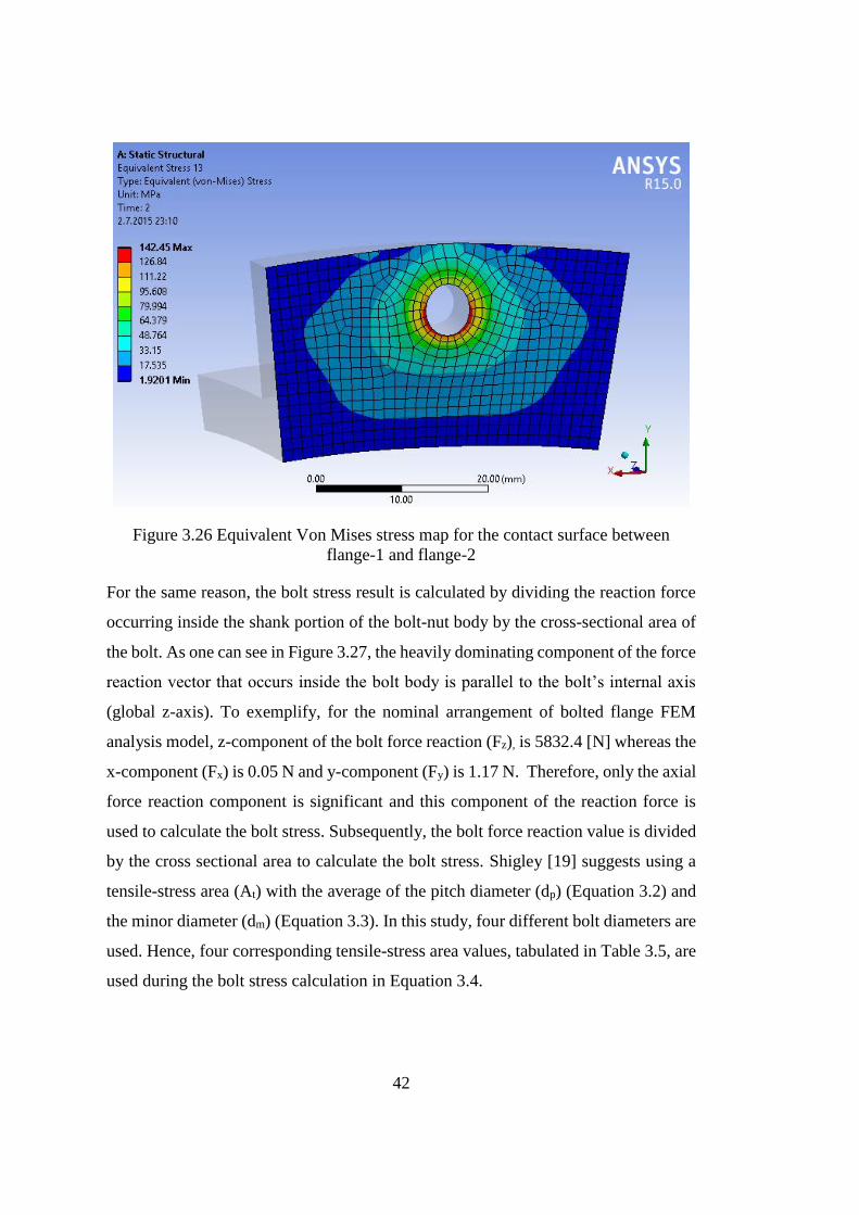
42

Figure 3.26 Equivalent Von Mises stress map for the contact surface between

flange-1 and flange-2

For the same reason, the bolt stress result is calculated by dividing the reaction force

occurring inside the shank portion of the bolt-nut body by the cross-sectional area of

the bolt. As one can see in Figure 3.27, the heavily dominating component of the force

reaction vector that occurs inside the bolt body is parallel to the bolt’s internal axis

(global z-axis). To exemplify, for the nominal arrangement of bolted flange FEM

analysis model, z-component of the bolt force reaction (Fz), is 5832.4 [N] whereas the

x-component (Fx) is 0.05 N and y-component (Fy) is 1.17 N. Therefore, only the axial

force reaction component is significant and this component of the reaction force is

used to calculate the bolt stress. Subsequently, the bolt force reaction value is divided

by the cross sectional area to calculate the bolt stress. Shigley [19] suggests using a

tensile-stress area (At) with the average of the pitch diameter (dp) (Equation 3.2) and

the minor diameter (dm) (Equation 3.3). In this study, four different bolt diameters are

used. Hence, four corresponding tensile-stress area values, tabulated in Table 3.5, are

used during the bolt stress calculation in Equation 3.4.

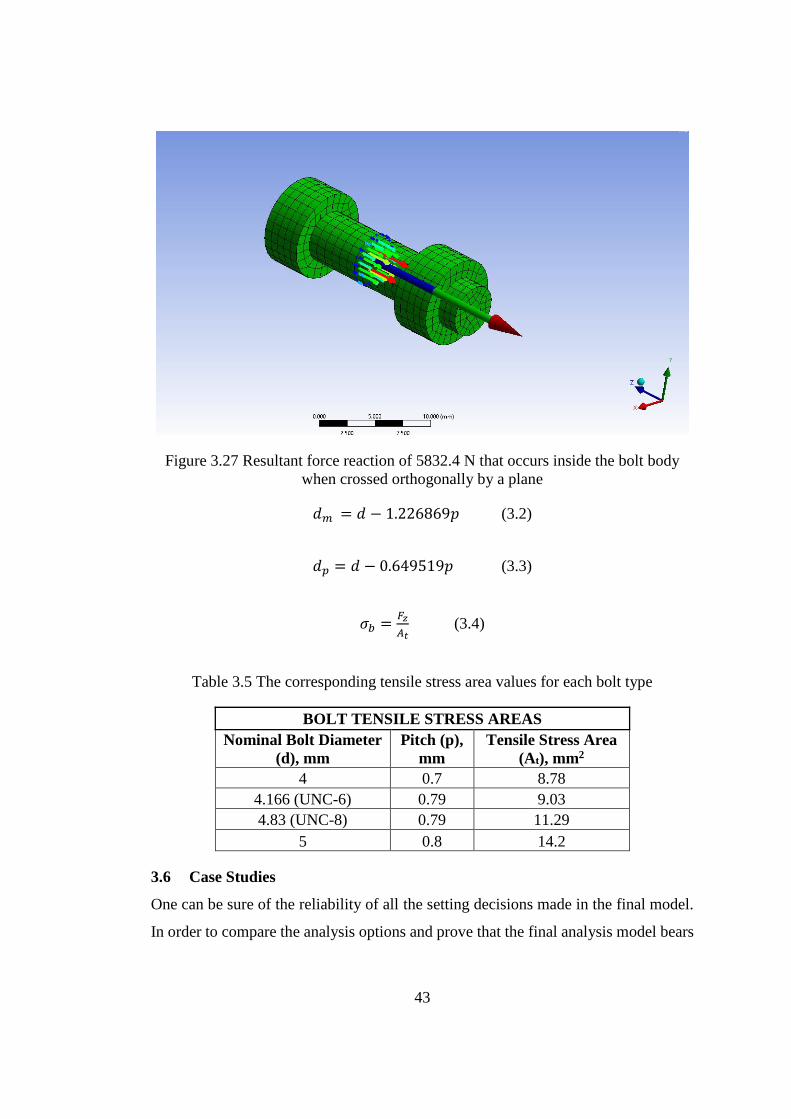
43

Figure 3.27 Resultant force reaction of 5832.4 N that occurs inside the bolt body

when crossed orthogonally by a plane

𝑑𝑚 = 𝑑 − 1.226869𝑝 (3.2)

𝑑𝑝 = 𝑑 − 0.649519𝑝 (3.3)

𝜎𝑏 =𝐹𝑧

𝐴𝑡 (3.4)

Table 3.5 The corresponding tensile stress area values for each bolt type

BOLT TENSILE STRESS AREAS

Nominal Bolt Diameter

(d), mm

Pitch (p),

mm

Tensile Stress Area

(At), mm2

4 0.7 8.78

4.166 (UNC-6) 0.79 9.03

4.83 (UNC-8) 0.79 11.29

5 0.8 14.2

3.6 Case Studies

One can be sure of the reliability of all the setting decisions made in the final model.

In order to compare the analysis options and prove that the final analysis model bears

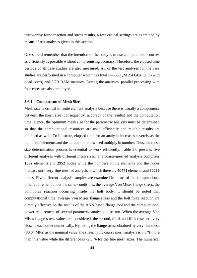
44

trustworthy force reaction and stress results, a few critical settings are examined by

means of test analyses given in this section.

One should remember that the intention of the study is to use computational sources

as efficiently as possible without compromising accuracy. Therefore, the elapsed time

periods of all case studies are also measured. All of the test analyses for the case

studies are performed in a computer which has Intel i7-3630QM 2.4 GHz CPU (with

quad cores) and 8GB RAM memory. During the analyses, parallel processing with

four cores are also employed.

3.6.1 Comparison of Mesh Sizes

Mesh size is critical in finite element analysis because there is usually a compromise

between the mesh size (consequently, accuracy of the results) and the computation

time. Hence, the optimum mesh size for the parametric analysis must be determined

so that the computational resources are used efficiently and reliable results are

obtained as well. To illustrate, elapsed time for an analysis increases severely as the

number of elements and the number of nodes used multiply in number. Thus, the mesh

size determination process is essential to work efficiently. Table 3.6 presents five

different analyses with different mesh sizes. The coarse-meshed analysis comprises

1582 elements and 2952 nodes while the numbers of the elements and the nodes

increase until very-fine-meshed analysis in which there are 40471 elements and 50266

nodes. Five different analysis samples are examined in terms of the computational

time requirement under the same conditions, the average Von Mises flange stress, the

bolt force reaction occurring inside the bolt body. It should be noted that

computational time, average Von Mises flange stress and the bolt force reaction are

directly effective on the results of the ANN based flange tool and the computational

power requirement of several parametric analysis to be run. When the average Von

Mises flange stress values are considered, the second, third, and fifth cases are very

close to each other numerically. By taking the flange stress obtained by very fine mesh

(80.04 MPa) as the nominal value, the stress in the coarse mesh analysis is 3.0 % more

than this value while the difference is -2.3 % for the fine mesh sizes. The numerical

45

variations between the cases of medium, medium-fine, and very fine mesh sizes are

about 1 %, which makes three of the mesh sizes acceptable for the calculation of the

average flange stress. Secondly, the nominal value of the bolt reaction force load can

be taken in somewhere close to 5837 N. In this respect, the coarse meshed analysis,

that is supposed to be the worst case among all, produces 0.4 % deviation from the

nominal value. Accordingly, all of the mesh sizes are acceptable for the bolt load

results. Lastly, the maximum total deformation value appears to be around 0.0468-

0.0489 [mm]. In the medium-fine, fine, and very fine meshed analyses, the results are

very close to each other (the maximum deviation is around 2 %). In the coarse and

medium size meshed analyses, slightly higher deviation is obtained compared to the

finest mesh case. Another point to be inspected is the average element qualities. The

picture is the same as with the previous situation since the last three mesh size cases

have very high element qualities. Last but not least, the elapsed time for each case

hugely differs. It takes 14 seconds to finish an analysis in the coarse meshed model

whereas the required time drastically increases to 293 seconds for the finest mesh case

in the same computer. In the present study, after evaluating all aspects, the medium-

fine mesh size with 11302 hexahedral elements and 15608 nodes is considered to be

the optimum mesh size for all parametric analyses considering the reliability of the

output and the computational power requirement.

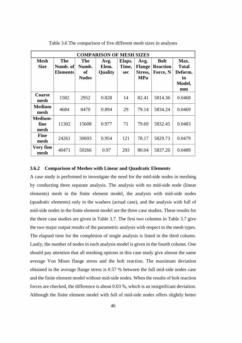
46

Table 3.6 The comparison of five different mesh sizes in analyses

COMPARISON OF MESH SIZES

Mesh

Size

The

Numb. of

Elements

The

Numb.

of

Nodes

Avg.

Elem.

Quality

Elaps.

Time,

sec

Avg.

Flange

Stress,

MPa

Bolt

Reaction

Force, N

Max.

Total

Deform.

in

Model,

mm

Coarse

mesh 1582 2952 0.828 14 82.41 5814.36 0.0468

Medium

mesh 4684 8470 0.894 29 79.14 5834.24 0.0469

Medium-

fine

mesh

11302 15608 0.977 71 79.69 5832.45 0.0483

Fine

mesh 24261 30693 0.954 121 78.17 5829.73 0.0479

Very fine

mesh 40471 50266 0.97 293 80.04 5837.26 0.0489

3.6.2 Comparison of Meshes with Linear and Quadratic Elements

A case study is performed to investigate the need for the mid-side nodes in meshing

by conducting three separate analysis. The analysis with no mid-side node (linear

elements) mesh in the finite element model, the analysis with mid-side nodes

(quadratic elements) only in the washers (actual case), and the analysis with full of

mid-side nodes in the finite element model are the three case studies. These results for

the three case studies are given in Table 3.7. The first two columns in Table 3.7 give

the two major output results of the parametric analysis with respect to the mesh types.

The elapsed time for the completion of single analysis is listed in the third column.

Lastly, the number of nodes in each analysis model is given in the fourth column. One

should pay attention that all meshing options in this case study give almost the same

average Von Mises flange stress and the bolt reaction. The maximum deviation

obtained in the average flange stress is 0.57 % between the full mid-side nodes case

and the finite element model without mid-side nodes. When the results of bolt reaction

forces are checked, the difference is about 0.03 %, which is an insignificant deviation.

Although the finite element model with full of mid-side nodes offers slightly better

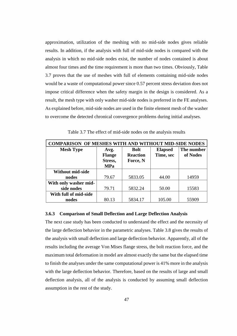
47

approximation, utilization of the meshing with no mid-side nodes gives reliable

results. In addition, if the analysis with full of mid-side nodes is compared with the

analysis in which no mid-side nodes exist, the number of nodes contained is about

almost four times and the time requirement is more than two times. Obviously, Table

3.7 proves that the use of meshes with full of elements containing mid-side nodes

would be a waste of computational power since 0.57 percent stress deviation does not

impose critical difference when the safety margin in the design is considered. As a

result, the mesh type with only washer mid-side nodes is preferred in the FE analyses.

As explained before, mid-side nodes are used in the finite element mesh of the washer

to overcome the detected chronical convergence problems during initial analyses.

Table 3.7 The effect of mid-side nodes on the analysis results

COMPARISON OF MESHES WITH AND WITHOUT MID-SIDE NODES

Mesh Type Avg.

Flange

Stress,

MPa

Bolt

Reaction

Force, N

Elapsed

Time, sec

The number

of Nodes

Without mid-side

nodes 79.67 5833.05 44.00 14959

With only washer mid-

side nodes 79.71 5832.24 50.00 15583

With full of mid-side

nodes 80.13 5834.17 105.00 55909

3.6.3 Comparison of Small Deflection and Large Deflection Analysis

The next case study has been conducted to understand the effect and the necessity of

the large deflection behavior in the parametric analyses. Table 3.8 gives the results of

the analysis with small deflection and large deflection behavior. Apparently, all of the

results including the average Von Mises flange stress, the bolt reaction force, and the

maximum total deformation in model are almost exactly the same but the elapsed time

to finish the analyses under the same computational power is 41% more in the analysis

with the large deflection behavior. Therefore, based on the results of large and small

deflection analysis, all of the analysis is conducted by assuming small deflection

assumption in the rest of the study.

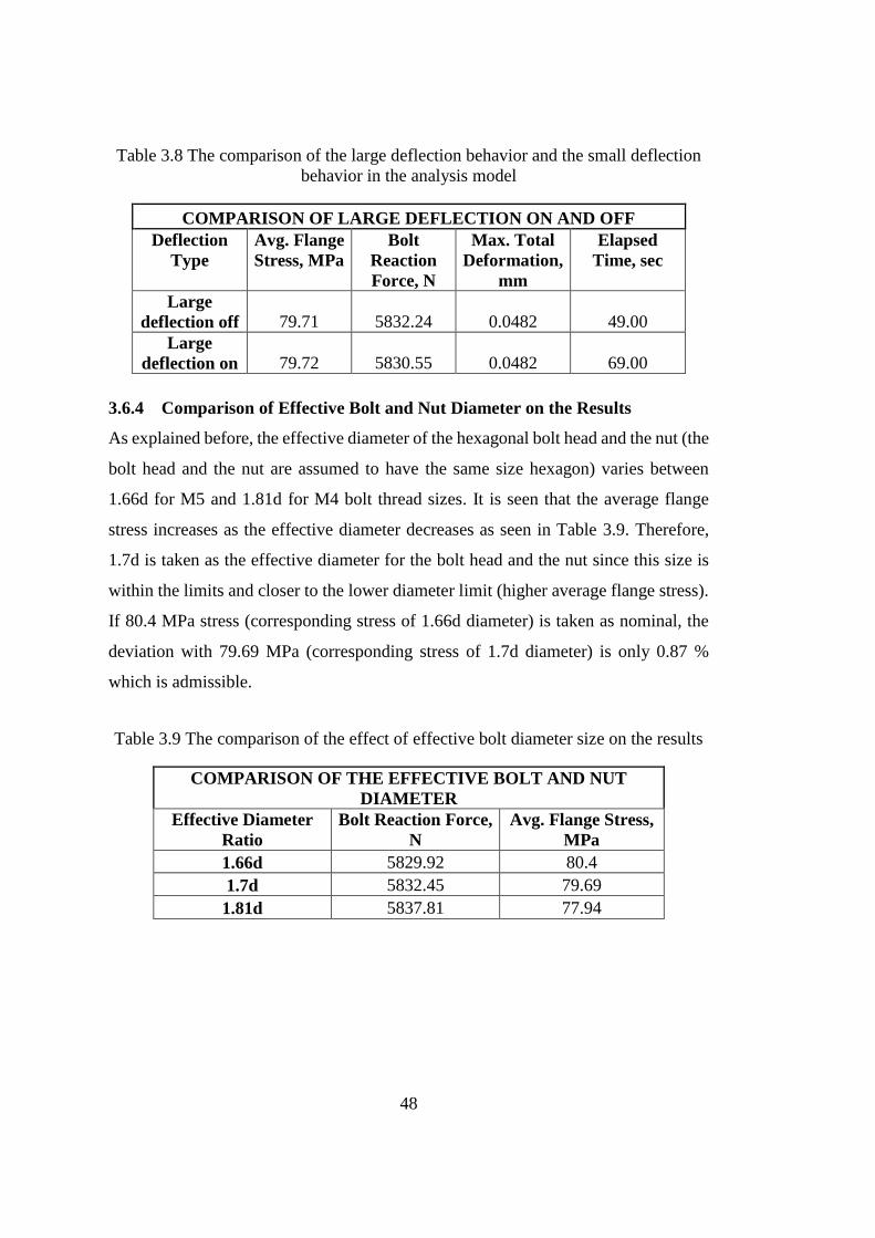
48

Table 3.8 The comparison of the large deflection behavior and the small deflection

behavior in the analysis model

COMPARISON OF LARGE DEFLECTION ON AND OFF

Deflection

Type

Avg. Flange

Stress, MPa

Bolt

Reaction

Force, N

Max. Total

Deformation,

mm

Elapsed

Time, sec

Large

deflection off 79.71 5832.24 0.0482 49.00

Large

deflection on 79.72 5830.55 0.0482 69.00

3.6.4 Comparison of Effective Bolt and Nut Diameter on the Results

As explained before, the effective diameter of the hexagonal bolt head and the nut (the

bolt head and the nut are assumed to have the same size hexagon) varies between

1.66d for M5 and 1.81d for M4 bolt thread sizes. It is seen that the average flange

stress increases as the effective diameter decreases as seen in Table 3.9. Therefore,

1.7d is taken as the effective diameter for the bolt head and the nut since this size is

within the limits and closer to the lower diameter limit (higher average flange stress).

If 80.4 MPa stress (corresponding stress of 1.66d diameter) is taken as nominal, the

deviation with 79.69 MPa (corresponding stress of 1.7d diameter) is only 0.87 %

which is admissible.

Table 3.9 The comparison of the effect of effective bolt diameter size on the results

COMPARISON OF THE EFFECTIVE BOLT AND NUT

DIAMETER

Effective Diameter

Ratio

Bolt Reaction Force,

N

Avg. Flange Stress,

MPa

1.66d 5829.92 80.4

1.7d 5832.45 79.69

1.81d 5837.81 77.94

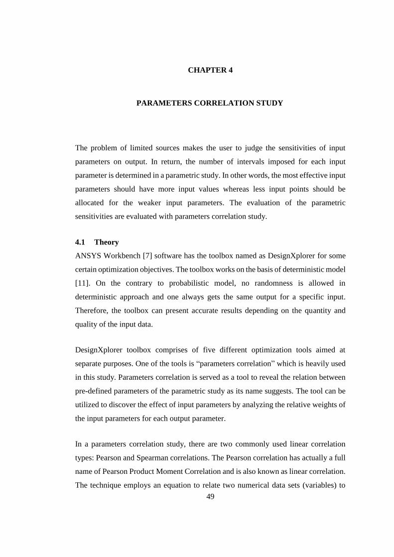
49

CHAPTER 4

PARAMETERS CORRELATION STUDY

The problem of limited sources makes the user to judge the sensitivities of input

parameters on output. In return, the number of intervals imposed for each input

parameter is determined in a parametric study. In other words, the most effective input

parameters should have more input values whereas less input points should be

allocated for the weaker input parameters. The evaluation of the parametric

sensitivities are evaluated with parameters correlation study.

4.1 Theory

ANSYS Workbench [7] software has the toolbox named as DesignXplorer for some

certain optimization objectives. The toolbox works on the basis of deterministic model

[11]. On the contrary to probabilistic model, no randomness is allowed in

deterministic approach and one always gets the same output for a specific input.

Therefore, the toolbox can present accurate results depending on the quantity and

quality of the input data.

DesignXplorer toolbox comprises of five different optimization tools aimed at

separate purposes. One of the tools is “parameters correlation” which is heavily used

in this study. Parameters correlation is served as a tool to reveal the relation between

pre-defined parameters of the parametric study as its name suggests. The tool can be

utilized to discover the effect of input parameters by analyzing the relative weights of

the input parameters for each output parameter.

In a parameters correlation study, there are two commonly used linear correlation

types: Pearson and Spearman correlations. The Pearson correlation has actually a full

name of Pearson Product Moment Correlation and is also known as linear correlation.

The technique employs an equation to relate two numerical data sets (variables) to

50

each other [34]. The result of this method gives the linear correlation between two

data sets and it takes numerical values ranging from “-1” to “1” indicating negative

and positive relations. Zero-value signifies the no-connection condition between two

numerical sets in Pearson correlation [34]. Spearman’s rank correlation coefficient is

one of the most commonly preferred nonparametric statistical technique [33] and it

evaluates the strength of the correlation between two parameters by comparing with a

monotonic function. In other words, if there is a perfectly monotonic increasing trend

between parameters, the Spearman correlation result is “+1”. On the other hand, the

relation between two parameters are perfect monotonic with inverse proportional

behavior, the Spearman correlation result is “-1”. Zero value again indicates no

relation between them [32]. The method is better in identifying non-linear, monotonic

relationships and less restrictive in comparison to linear methods [11]. Hence,

Spearman correlation method is selected in this study because of having non-linear

analysis model. In both Pearson correlation and Spearman’s rank correlation

techniques, the values changing from 0.5 to 1 are the sign of highly proportional

relations while the values in between -0.5 to -1 denote strong inverse-proportional

relations between two data sets [32, 34].

To express better, two data sets and their Spearman’s rank correlation is considered

in Table 4.1. Set-1 and set-2 consist of three randomly selected elements. Rank-1 is

created by giving corresponding numbers starting from 1 for the smallest element to

3 for the largest element in the increasing order considering the sequence of the

elements’ numerical values. In the same way, rank of the set-2 is also formed (rank-

2) in consideration to the element numerical value sequence. “𝑑” is the difference of

rank-1 and rank-2. In the last column of Table 4.1 shows square of 𝑑. The Spearman’s

rank correlation is represented by Equation 4.1, in which “𝑛” is the number of samples

in each set (𝑛 = 3 in this example) and “𝑟” is the correlation coefficient of set-1 and

set-2.

51

Table 4.1 Sample problem data of Spearman’s rank correlation

Set-1 Set-2 Rank-1 Rank-2 d d2

7 4 2 1 1 1

6 15 1 3 -2 4

11 5 3 2 1 1

𝑟 = 1 − (6 ∙ ∑𝑑2

𝑛(𝑛2 − 1)) (4.1)

𝑟 = −0.5 (4.2)

The results of the parametric study are exhibited in different forms by parameters

correlation tool in ANSYS. The first type is correlation matrix. There are two options

to exhibit the results of the correlation matrix. Correlation matrix with numerical

values and its visual chart form expressing the same relation are the two options

available. Correlation matrix explains linear correlation between each input-output

pair. In matrix form, the values towards “1” indicate increasing linearity while the

values approaching “-1” are interpreted as inversely linear relations. In other words,

the coefficients in the correlation matrix are the indicators of the correlation direction

and the grade. In the same way, the visual chart expresses the same relations with

colors. In the second form, the same linear relationships are shown as bar or pie chart

for each output parameter separately so that the global effects of input parameters on

a specific output can be compared easily. In the sensitivities chart, correlation matrix

is displayed for each output parameter separately.

4.2 Method

Development of bolted flange design tool is based on the FEM analysis database of

13500 analyses. If the total number of analyses is limited due to computational power,

determination of the number of input values for each parameter is very crucial. If the

number of input values for each parameter is increased, then total number of finite

element analysis increases significantly because total number of analysis is obtained

by the product of the number of input values of each parameter.

52

In this study, apart from the main parametric study to create the database, parametric

analyses performed are to investigate the sensitivities of input parameters on the

output and to compare them with each other to decide on the number of input values

to be used for the main parametric analyses. In ANSYS Workbench under the

“DesignXplorer” toolbox “Parameters Correlation” tool that exists is used for the

purpose of determining the parameter sensitivities. The correlation strengths between

the input and the output parameters are displayed both visually and numerically.

As stated in previous section, there are seven input parameters, five of which are

geometric variables and the remaining ones are the loading variables. Without doubt,

the loading variables have direct effect on the force and the stress results on the bolt

and the flanges. However, the difficulty is to determine the sensitivities of the

geometric variables due to the fact that the geometric variables do not have obvious

linear effects on the output, rather they affect the equivalent flange and the equivalent

bolt stiffness values. Since the theoretical approach for the calculation of the stiffness

values are mostly based on the assumptions, the actual effects of the geometric input

parameters on the output results are not clearly disclosed. Consequently, the

parametric analysis study with parameters correlation is conducted for the geometric

variables. Thus, the sensitivities of the geometric input variables on the output results

are compared with each other to make a correct decision about the number of input

intervals for each geometric design variable.

Parameters correlation study comprises certain steps. Firstly, the geometric variables

of the bolted flange connection and the loading input containing the bolt pretension

and the axial external force are defined with the nominal values. The parametric input

values in each parametric set consisting of 100 FE analyses are specifically

determined by ANSYS algorithms so that the selected input values are evenly

distributed within the pre-defined lower and upper limits of the input parameters [11].

The sample generation algorithm prevents the overlaps of the input values while

selecting the samples for correlations [11]. The values are transferred to ANSYS

DesignModeler toolbox [7] to create 3D FEM analysis geometry. In the next step, the

53

created analysis geometry with respect to the selected sample points is sent to static

structural FEM analysis. Here, the meshing operation of the parts is made consistent

with the predefined meshing settings and the analysis is performed in the end. These

steps are repeated in an automated way until one hundred analyses are finished to form

a parametric set for the parameters correlation study. Once the parametric set is ready,

parameters correlation study can be performed to understand the relation between the

selected input parameters and the output. One can see the flowchart of the parameters

correlation study procedure in Figure 4.1.

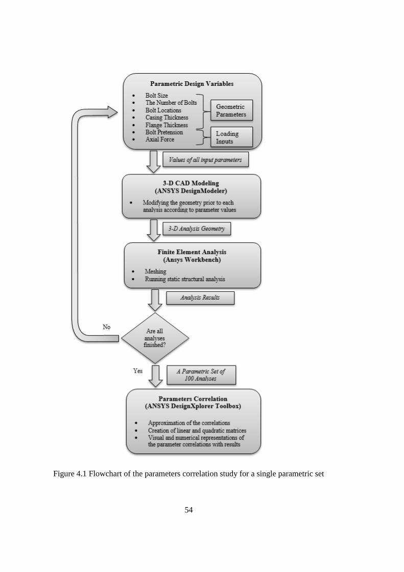
54

Figure 4.1 Flowchart of the parameters correlation study for a single parametric set

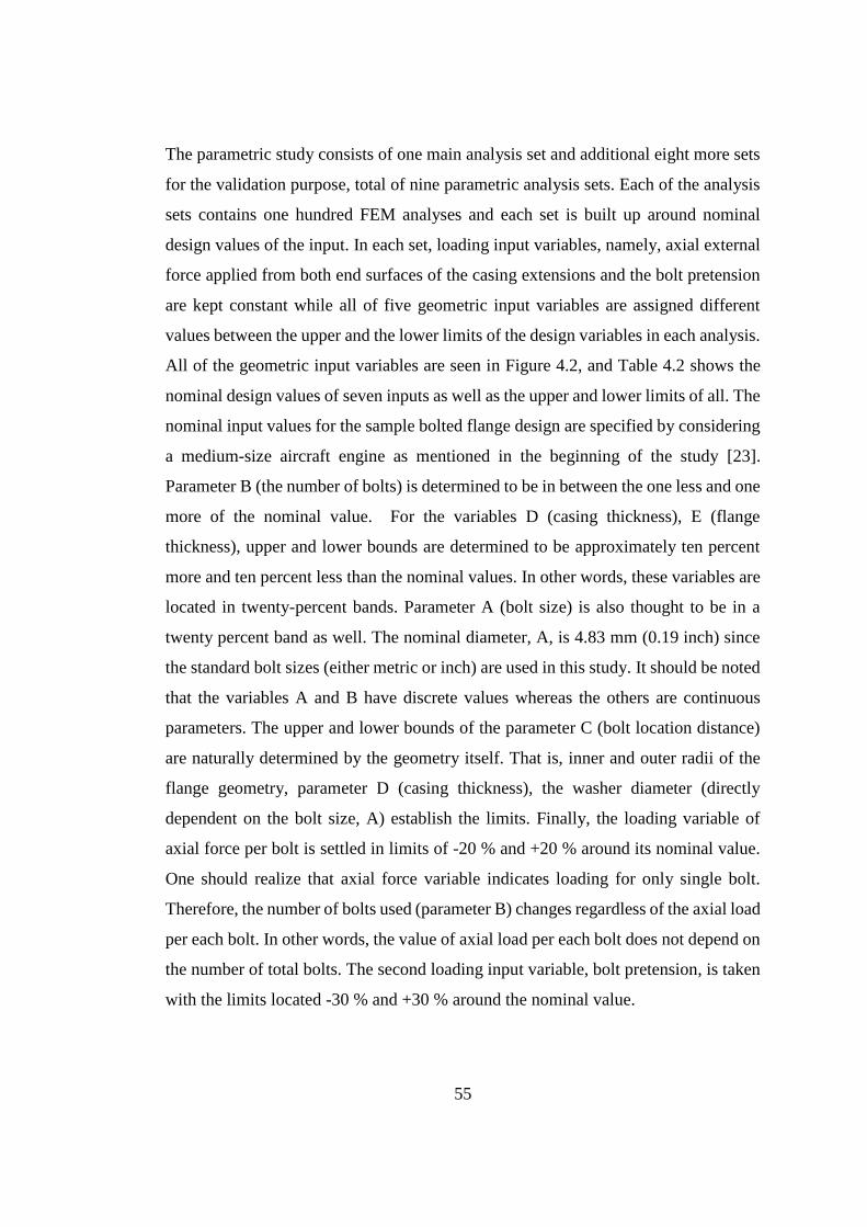
55

The parametric study consists of one main analysis set and additional eight more sets

for the validation purpose, total of nine parametric analysis sets. Each of the analysis

sets contains one hundred FEM analyses and each set is built up around nominal

design values of the input. In each set, loading input variables, namely, axial external

force applied from both end surfaces of the casing extensions and the bolt pretension

are kept constant while all of five geometric input variables are assigned different

values between the upper and the lower limits of the design variables in each analysis.

All of the geometric input variables are seen in Figure 4.2, and Table 4.2 shows the

nominal design values of seven inputs as well as the upper and lower limits of all. The

nominal input values for the sample bolted flange design are specified by considering

a medium-size aircraft engine as mentioned in the beginning of the study [23].

Parameter B (the number of bolts) is determined to be in between the one less and one

more of the nominal value. For the variables D (casing thickness), E (flange

thickness), upper and lower bounds are determined to be approximately ten percent

more and ten percent less than the nominal values. In other words, these variables are

located in twenty-percent bands. Parameter A (bolt size) is also thought to be in a

twenty percent band as well. The nominal diameter, A, is 4.83 mm (0.19 inch) since

the standard bolt sizes (either metric or inch) are used in this study. It should be noted

that the variables A and B have discrete values whereas the others are continuous

parameters. The upper and lower bounds of the parameter C (bolt location distance)

are naturally determined by the geometry itself. That is, inner and outer radii of the

flange geometry, parameter D (casing thickness), the washer diameter (directly

dependent on the bolt size, A) establish the limits. Finally, the loading variable of

axial force per bolt is settled in limits of -20 % and +20 % around its nominal value.

One should realize that axial force variable indicates loading for only single bolt.

Therefore, the number of bolts used (parameter B) changes regardless of the axial load

per each bolt. In other words, the value of axial load per each bolt does not depend on

the number of total bolts. The second loading input variable, bolt pretension, is taken

with the limits located -30 % and +30 % around the nominal value.

56

Figure 4.2 The geometric input parameters of the analysis model

Table 4.2 The nominal values, upper and lower limits of all input parameters

Input Variable Explanation Nominal

Value

Lower

Bound

Upper

Bound A Bolt Size 4.83 mm 4 mm 5 mm

B The Number of Bolts 24 pcs 23 pcs 25 pcs

C Bolt Location 167.75

mm

mm[mm]

164.5 mm 168.9 mm

D Casing Thickness 6.6 mm 5.9 mm 7.3 mm

E Flange Thickness 5 mm 4.5 mm 5.5 mm

Axial Force per

Bolt

- 1280 N 1024 N 1536 N

Bolt Pretension - 5702 N 3991 N 7413 N

Normally, the parameters correlation results are analyzed for single set of one-

hundred analyses by keeping the axial force and the bolt pretension constant. To be

on the safe side, the axial force and bolt pretension parameters are also intended to be

crossed with their three different values (nominal, upper limit, and lower limit values

of each) so that the effect of having different constant loading values on the geometric

parameter correlation study could also be investigated. The main analysis set with

nominal loading values is listed in the first row of Table 4.3. Eight supplementary

parametric sets are also listed with the loading input parameters in Table 4.3. The

expected result is to obtain approximately the same correlation strengths of the

geometric parameters on the output parameters regardless of the loading conditions in

all the sets.

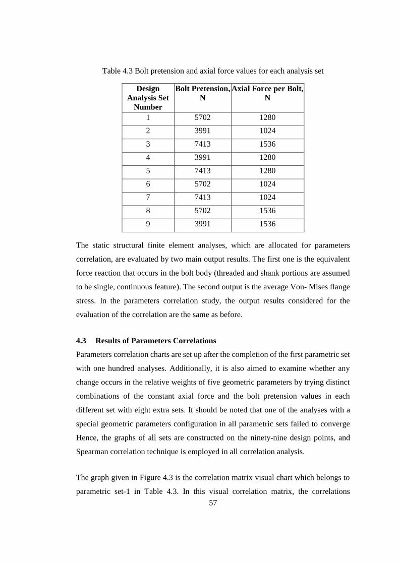
57

Table 4.3 Bolt pretension and axial force values for each analysis set

Design

Analysis Set

Number

Bolt Pretension,

N

Axial Force per Bolt,

N

1 5702 1280

2 3991 1024

3 7413 1536

4 3991 1280

5 7413 1280

6 5702 1024

7 7413 1024

8 5702 1536

9 3991 1536

The static structural finite element analyses, which are allocated for parameters

correlation, are evaluated by two main output results. The first one is the equivalent

force reaction that occurs in the bolt body (threaded and shank portions are assumed

to be single, continuous feature). The second output is the average Von- Mises flange

stress. In the parameters correlation study, the output results considered for the

evaluation of the correlation are the same as before.

4.3 Results of Parameters Correlations

Parameters correlation charts are set up after the completion of the first parametric set

with one hundred analyses. Additionally, it is also aimed to examine whether any

change occurs in the relative weights of five geometric parameters by trying distinct

combinations of the constant axial force and the bolt pretension values in each

different set with eight extra sets. It should be noted that one of the analyses with a

special geometric parameters configuration in all parametric sets failed to converge

Hence, the graphs of all sets are constructed on the ninety-nine design points, and

Spearman correlation technique is employed in all correlation analysis.

The graph given in Figure 4.3 is the correlation matrix visual chart which belongs to

parametric set-1 in Table 4.3. In this visual correlation matrix, the correlations

58

between design parameters are represented with the colors indicating the strength

levels. The red color means the highest proportional correlation of “1” between two

variables while the blue color is the indicator for the highest inversely proportional

relation between two parameters. The combination of any parameter with itself is

always designated with the full red color, which means the direct relation of a

parameter with itself. The rest of the colors are expressed in the color map of Figure

4.3. The visual correlation chart is useful to show the effect of the input parameters

on the results at a glance. The locations of the parameters in the charts are not related

with the importance level and are defined by the software. The same parameters are

located in both the row and the column in the same sequence. According to Figure

4.3, the most effective input variable is the bolt location distance from the center axis

(parameter C) with a strong linear correlation for the bolt force reaction result. The

bolt size used (parameter A) has a weak, increasing effect whereas the casing

thickness (parameter D) and the flange thickness (parameter E) display weak

decreasing effect on the bolt reaction force. When the second output result, the

average equivalent flange stress, is considered, the parameters A and C are

remarkable. As the bolt size (parameter A) enlarges, the average flange stress

diminishes. On the other hand, the increase in the bolt location distance (parameter C)

increases the average flange stress. The number of bolts (parameter B) seems to have

almost no effect on the results. However, one should pay attention that the changes in

the number of bolts does not affect the corresponding portion of the axial external

force applied to the whole flange. The axial force applied to the circular sector flange

model is constant in the parameters correlation study. In other words, the change in

the number of bolts used in the fully circular flange assembly only changes the angle

of the flange sector arc. Table 4.4 is the numerical representation of the same linear

correlation matrix. The correlation weight more than 0.5 or less than -0.5 are painted

in red color in Table 4.4. If the correlations of the parameters with themselves or the

correlations of the output parameters with each other are omitted, the remaining red

cells are the critical ones designated with bold letters.

59

Figure 4.3 Visual chart of the correlation matrix of parametric set-1

60

Table 4.4 The correlation matrix of parametric set-1

CORRELATION MATRIX (LINEAR)

Parameters B A E C D Bolt

Load

Avg. Flng.

Stress

B 1.000 -0.010 -0.009 0.003 0.018 0.089 -0.009

A -0.010 1.000 0.001 0.012 -0.008 0.261 -0.667

E -0.009 0.001 1.000 -0.010 -0.006 -0.316 -0.363

C 0.003 0.012 -0.010 1.000 0.004 0.855 0.603

D 0.018 -0.008 -0.006 0.004 1.000 -0.297 -0.143

Bolt Load 0.089 0.261 -0.316 0.855 -0.297 1.000 0.502

Avg. Flng.

Stress

-0.009 -0.667 -0.363 0.603 -0.143 0.502 1.000

The correlation matrix results can also be evaluated by considering the sensitivities

chart in Figure 4.4 since the sensitivities chart is another representation type of the

correlation matrix in order to display the global sensitivities of output parameters [11].

The dominant design parameters on the output parameters explained above are clearly

seen in the sensitivities chart.

61

Figure 4.4 The sensitivities chart of parametric set-1

When the results of the correlation study for the main parametric set are examined,

parameter C stands out as the most critical factor for the bolt load output. Parameters

E and D exhibit relatively low relations on the bolt load. Parameters A has a slightly

lower correlation with bolt load. Parameter B has almost no effect on the bolt load.

On the other hand, parameters A and C together seem to have noteworthy effects on

the average flange stress result. Parameter E comes in the third place in terms its effect

on the average flange stress. Parameters B and D do not have profound effect on the

average flange stress.

The results considered in Figures 4.3, 4.4 and Table 4.4 present that the bolt location

(parameter C) has a very strong proportional impact on the bolt reaction force as well

as on the average Von Mises flange stress. Therefore, parameter C is accepted to be

the most critical geometric parameter in this study. Bolt size (parameter A) is the

second crucial geometric parameter since it has strong inversely proportional effect

on the average Von Mises flange stress output. The flange thickness (parameter E) is

slightly more effective than the casing thickness (parameter D) on the output by

62

considering the coefficients. Finally, the number of bolts (parameter B) has almost no

effect on the output when the first column of the correlation matrix is considered. One

should pay attention that a portion of total axial external force is applied constantly to

the structure throughout the parameters correlation study. Therefore, the change of the

number of bolts affects only the angle of the circular sector while the applied force is

always constant in this study. This is why parameter B looks ineffective here. In the

final bolted flange design tool, the change in parameter B is going to directly affect

the corresponding axial force on the sectional analysis geometry.

In the final step of the parameters correlation study, the significance of the geometric

parameters are found to be in the following order: C > A > E > D > B.

The results of the parameters correlation study with a parametric set of 100 analyses

are checked by repeating the study for the same parameters with a set of 200 analyses.

It is seen that the parameters correlation study with 200 FE analyses gives almost the

same correlation coefficients. Therefore, the importance levels of the geometric input

parameters are sorted in the same order.

The number of values of the parameters to be used in building the ANN model are

determined by considering the outcome of the parameters correlation study. Table 4.5

shows the number of input values for each design variable to be used in the parametric

analysis as design points. Two load variables and one geometric parameter (parameter

C, bolt location) are the most effective parameters on the output. Therefore, five

design points are allocated to them. For the geometric parameters E, D, B, three design

points are allocated as seen in Table 4.5. In the final parametric set, there are 13500

separate FE analyses when all of the input parameters are combined with each other.

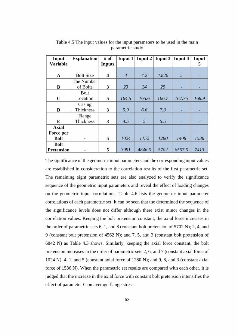
63

Table 4.5 The input values for the input parameters to be used in the main

parametric study

Input

Variable

Explanation # of

Inputs

Input 1 Input 2 Input 3 Input 4 Input

5

A Bolt Size 4 4 4.2 4.826 5 -

B

The Number

of Bolts 3 23 24 25 - -

C

Bolt

Location 5 164.5 165.6 166.7 167.75 168.9

D

Casing

Thickness 3 5.9 6.6 7.3 - -

E

Flange

Thickness 3 4.5 5 5.5 - -

Axial

Force per

Bolt - 5 1024 1152 1280 1408 1536

Bolt

Pretension - 5 3991 4846.5 5702 6557.5 7413

The significance of the geometric input parameters and the corresponding input values

are established in consideration to the correlation results of the first parametric set.

The remaining eight parametric sets are also analyzed to verify the significance

sequence of the geometric input parameters and reveal the effect of loading changes

on the geometric input correlations. Table 4.6 lists the geometric input parameter

correlations of each parametric set. It can be seen that the determined the sequence of

the significance levels does not differ although there exist minor changes in the

correlation values. Keeping the bolt pretension constant, the axial force increases in

the order of parametric sets 6, 1, and 8 (constant bolt pretension of 5702 N); 2, 4, and

9 (constant bolt pretension of 4562 N); and 7, 5, and 3 (constant bolt pretension of

6842 N) as Table 4.3 shows. Similarly, keeping the axial force constant, the bolt

pretension increases in the order of parametric sets 2, 6, and 7 (constant axial force of

1024 N); 4, 1, and 5 (constant axial force of 1280 N); and 9, 8, and 3 (constant axial

force of 1536 N). When the parametric set results are compared with each other, it is

judged that the increase in the axial force with constant bolt pretension intensifies the

effect of parameter C on average flange stress.

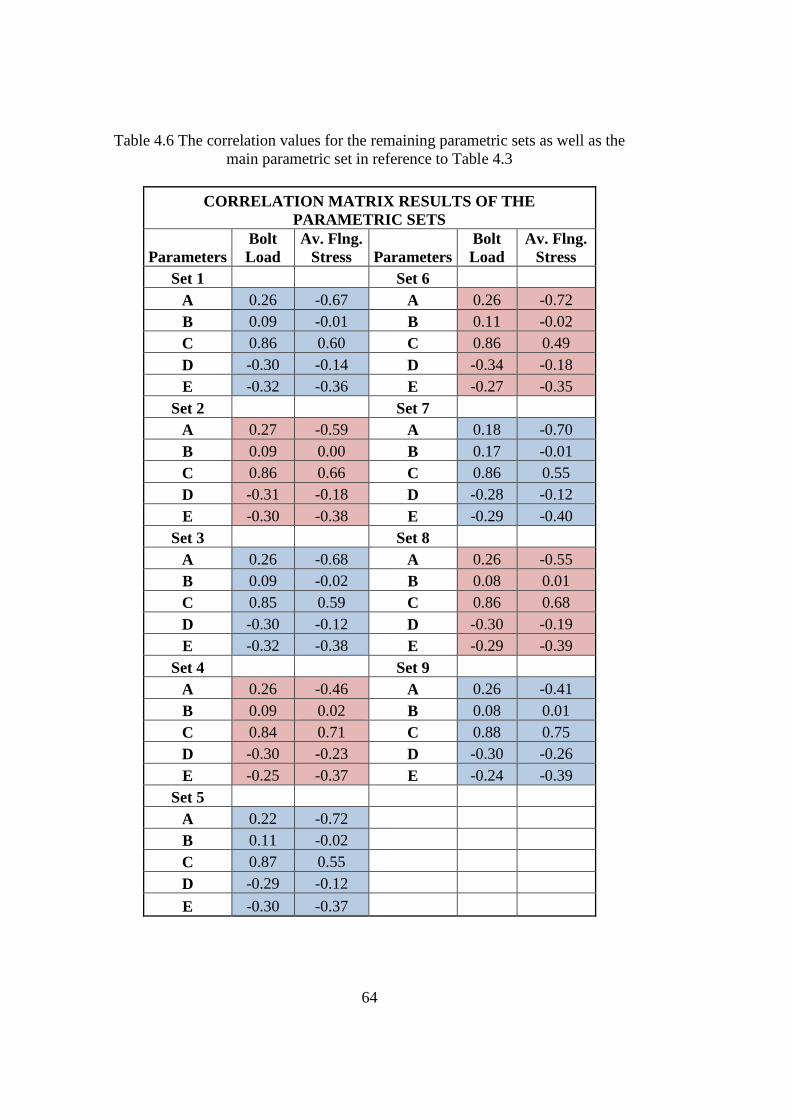
64

Table 4.6 The correlation values for the remaining parametric sets as well as the

main parametric set in reference to Table 4.3

CORRELATION MATRIX RESULTS OF THE

PARAMETRIC SETS

Parameters

Bolt

Load

Av. Flng.

Stress Parameters

Bolt

Load

Av. Flng.

Stress

Set 1 Set 6

A 0.26 -0.67 A 0.26 -0.72

B 0.09 -0.01 B 0.11 -0.02

C 0.86 0.60 C 0.86 0.49

D -0.30 -0.14 D -0.34 -0.18

E -0.32 -0.36 E -0.27 -0.35

Set 2 Set 7

A 0.27 -0.59 A 0.18 -0.70

B 0.09 0.00 B 0.17 -0.01

C 0.86 0.66 C 0.86 0.55

D -0.31 -0.18 D -0.28 -0.12

E -0.30 -0.38 E -0.29 -0.40

Set 3 Set 8

A 0.26 -0.68 A 0.26 -0.55

B 0.09 -0.02 B 0.08 0.01

C 0.85 0.59 C 0.86 0.68

D -0.30 -0.12 D -0.30 -0.19

E -0.32 -0.38 E -0.29 -0.39

Set 4 Set 9

A 0.26 -0.46 A 0.26 -0.41

B 0.09 0.02 B 0.08 0.01

C 0.84 0.71 C 0.88 0.75

D -0.30 -0.23 D -0.30 -0.26

E -0.25 -0.37 E -0.24 -0.39

Set 5

A 0.22 -0.72

B 0.11 -0.02

C 0.87 0.55

D -0.29 -0.12

E -0.30 -0.37

65

CHAPTER 5

ARTIFICIAL NEURAL NETWORK APPROXIMATION

5.1 Theory

Artificial neural networks are the computational structures with several computational

cells to solve especially complex, non-linear or stochastic problems by employing

simple, self-organizing algorithm. The artificial neural network (ANN) mechanism

works on the principles of the biological nerve system (neural network) of human

[29]. The characteristic properties are the capabilities of organizing, generalizing,

classifying, and learning data [30].

The dynamic structure of the network is formed by a group of processing units called

neurons, in which each neuron has connections with all of the neurons located in the

previous and next layers with different weights defined in the training [18]. Figure 5.1

represents an ANN network structure. In this network, there are three input parameters

taken from the input layer terminals and two output parameters sent through the output

layer terminals. The hidden layer is formed by four processing neurons. Therefore,

the structure of the ANN in Figure 5.1 is nominated as 3:4:2 architecture. Since the

input and output layers can only transmit the data, the capability of an ANN is adjusted

with the number of hidden layers and the number of neurons in each layer and this is

a trial and error method [30]. Each neuron in a layer has connections with all the

neurons located in the previous and the next layers. The strength of a connection

between a specific neuron pair is known as “weight”. The weights are defined in the

training operation.

66

Figure 5.1 The structure of a sample ANN with three input and two output

parameters

The training of artificial neural network operation is carried out in six phases which

consist of creating the network, configuring the network, initializing the weights and

biases, training the network, validating the network, and using the network in

sequence [22].

In the neural network toolbox of Matlab, there are four main neural network tools.

The first tool is “function fitting”. In this tool, it is possible to train neural networks

in different architectures in order to fit any kind of function. “Pattern recognition” tool

is the next one in neural network toolbox, which is employed for detecting object and

classifying the input data based on intended data properties. Another tool in the

toolbox is “data clustering”. Data clustering is used to group data by considering

similarities. The fourth tool is “time series analysis”, in which a neural network with

a dynamic behavior is employed to forecast the future activities by looking at the past

data. In this study, the function fitting tool is employed for approximation.

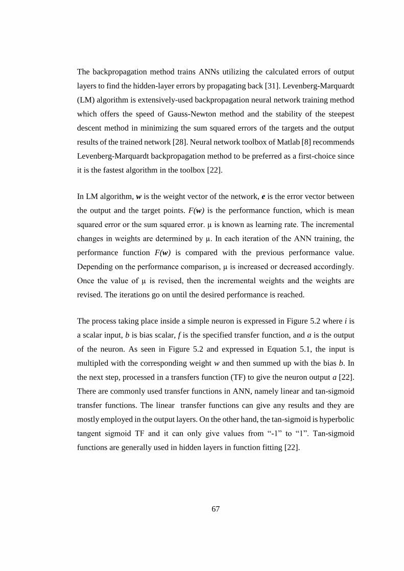
67

The backpropagation method trains ANNs utilizing the calculated errors of output

layers to find the hidden-layer errors by propagating back [31]. Levenberg-Marquardt

(LM) algorithm is extensively-used backpropagation neural network training method

which offers the speed of Gauss-Newton method and the stability of the steepest

descent method in minimizing the sum squared errors of the targets and the output

results of the trained network [28]. Neural network toolbox of Matlab [8] recommends

Levenberg-Marquardt backpropagation method to be preferred as a first-choice since

it is the fastest algorithm in the toolbox [22].

In LM algorithm, w is the weight vector of the network, e is the error vector between

the output and the target points. F(w) is the performance function, which is mean

squared error or the sum squared error. µ is known as learning rate. The incremental

changes in weights are determined by µ. In each iteration of the ANN training, the

performance function F(w) is compared with the previous performance value.

Depending on the performance comparison, µ is increased or decreased accordingly.

Once the value of µ is revised, then the incremental weights and the weights are

revised. The iterations go on until the desired performance is reached.

The process taking place inside a simple neuron is expressed in Figure 5.2 where i is

a scalar input, b is bias scalar, f is the specified transfer function, and a is the output

of the neuron. As seen in Figure 5.2 and expressed in Equation 5.1, the input is

multipled with the corresponding weight w and then summed up with the bias b. In

the next step, processed in a transfers function (TF) to give the neuron output a [22].

There are commonly used transfer functions in ANN, namely linear and tan-sigmoid

transfer functions. The linear transfer functions can give any results and they are

mostly employed in the output layers. On the other hand, the tan-sigmoid is hyperbolic

tangent sigmoid TF and it can only give values from “-1” to “1”. Tan-sigmoid

functions are generally used in hidden layers in function fitting [22].

68

Figure 5.2 The mathematical process in a simple neuron

𝑎 = 𝑓(𝑤 ∙ 𝑖 + 𝑏) (5.1)

The artificial neural networks can be adapted to find solution for wide range of

problems including function fitting, pattern recognition, data-mining, prediction,

detection, clustering, etc. Moreover, the problems can be non-analytical, non-linear,

stochastic, non-stationary, etc. Another major advantage of the artificial neural

network is the capability of solving complicated problems without serious

requirement of specially programming for a specific problem. The ANN methodology

eliminates the need of having heavy mathematical background of a problem. Thus,

the methodology can be utilized by everyone instead of by only experts in that area

[29].

5.2 The Artificial Neural Network Generation Process

Having a successfully trained ANN is heavily related with having sufficient data

points in the supplied database. For this purpose, a parametric database of 13500

design points (analyses) are employed. The parametric set of 13500 analyses are

divided into 25 equal sets in order to manage the analysis better. In the end of the

analyses, there are 25 parametric sets with the tabulated results in the form of

spreadsheet. Each set consists of 540 separate FE analyses. All of the design points

succeeded in converging to a solution.

After the completion of all analyses, the solution results are post processed for ANN

training. Firstly, twenty five spreadsheets in ANSYS are exported to Microsoft Excel

[27] by hand. Each analysis set containing input and output values is placed to distinct

sheets in the file. A script is prepared to collect the spreadsheets from Excel and

concatenate the twenty five separate matrices into a single matrix.

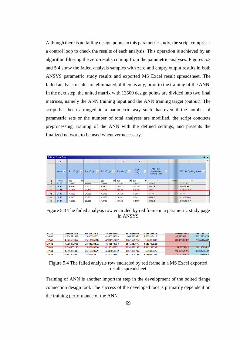
69

Although there is no failing design points in this parametric study, the script comprises

a control loop to check the results of each analysis. This operation is achieved by an

algorithm filtering the zero-results coming from the parametric analyses. Figures 5.3

and 5.4 show the failed-analysis samples with zero and empty output results in both

ANSYS parametric study results and exported MS Excel result spreadsheet. The

failed analysis results are eliminated, if there is any, prior to the training of the ANN.

In the next step, the united matrix with 13500 design points are divided into two final

matrices, namely the ANN training input and the ANN training target (output). The

script has been arranged in a parametric way such that even if the number of

parametric sets or the number of total analyses are modified, the script conducts

preprocessing, training of the ANN with the defined settings, and presents the

finalized network to be used whenever necessary.

Figure 5.3 The failed analysis row encircled by red frame in a parametric study page

in ANSYS

Figure 5.4 The failed analysis row encircled by red frame in a MS Excel exported

results spreadsheet

Training of ANN is another important step in the development of the bolted flange

connection design tool. The success of the developed tool is primarily dependent on

the training performance of the ANN.

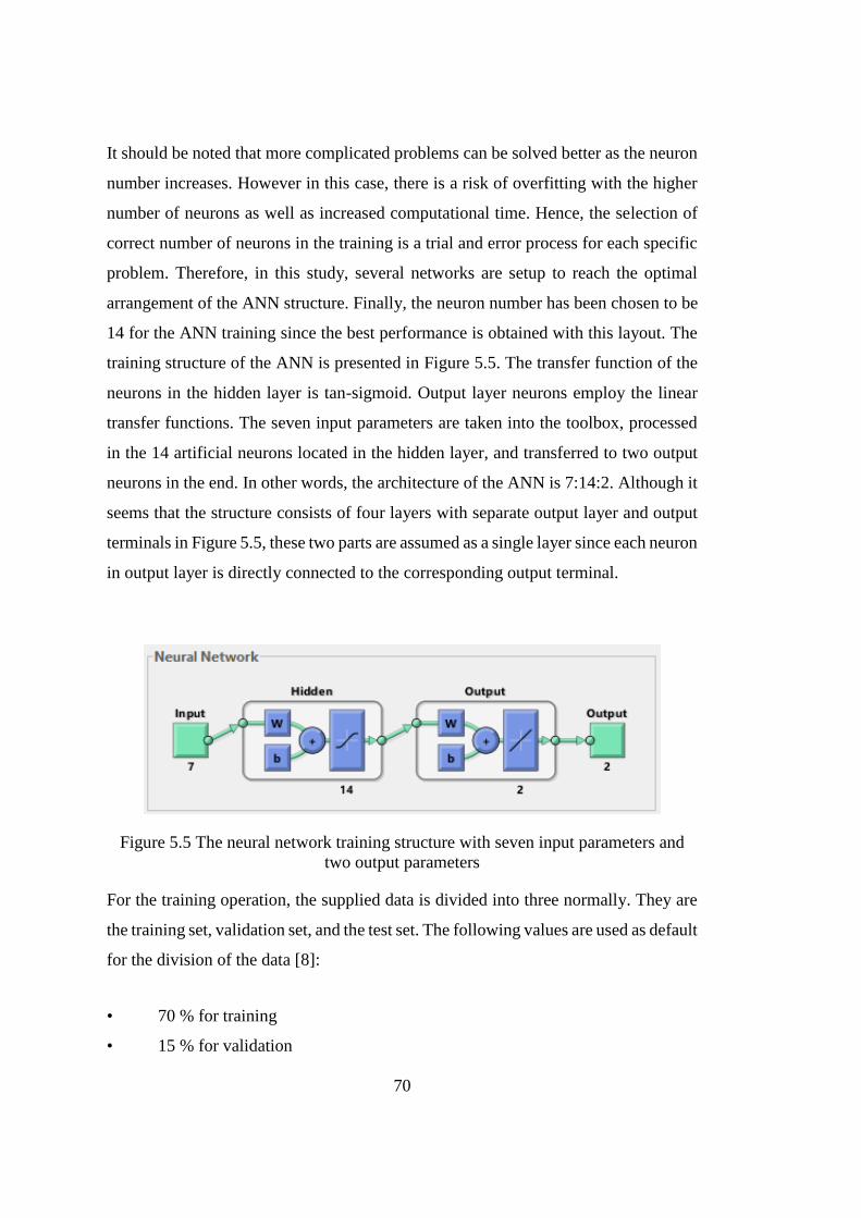
70

It should be noted that more complicated problems can be solved better as the neuron

number increases. However in this case, there is a risk of overfitting with the higher

number of neurons as well as increased computational time. Hence, the selection of

correct number of neurons in the training is a trial and error process for each specific

problem. Therefore, in this study, several networks are setup to reach the optimal

arrangement of the ANN structure. Finally, the neuron number has been chosen to be

14 for the ANN training since the best performance is obtained with this layout. The

training structure of the ANN is presented in Figure 5.5. The transfer function of the

neurons in the hidden layer is tan-sigmoid. Output layer neurons employ the linear

transfer functions. The seven input parameters are taken into the toolbox, processed

in the 14 artificial neurons located in the hidden layer, and transferred to two output

neurons in the end. In other words, the architecture of the ANN is 7:14:2. Although it

seems that the structure consists of four layers with separate output layer and output

terminals in Figure 5.5, these two parts are assumed as a single layer since each neuron

in output layer is directly connected to the corresponding output terminal.

Figure 5.5 The neural network training structure with seven input parameters and

two output parameters

For the training operation, the supplied data is divided into three normally. They are

the training set, validation set, and the test set. The following values are used as default

for the division of the data [8]:

• 70 % for training

• 15 % for validation

71

• 15 % for testing.

The training set is used for only in training of the weights and biases between the

neurons. Validation set is not employed in training but utilized for the validation

purpose in the end of every training iteration to terminate the training process. Test

set is completely unconnected with the training operation. The test samples are

employed in order to check the performance of the finalized network. It should be

noted that the validation and test sets are not processed in the training operation. In

this study, the complete database of 13500 samples are divided into three sets as

follows:

• 90 % for training

• 5 % for validation

• 5 % for testing.

In the construction of the ANN, the samples are assigned to each set randomly

according to the percentages. In the training process, the performance criterion is

taken as the mean squared error. In calculation of the mean squared error, the

importance of all targets are equal to each other as a default setting. Therefore, the

elements in error matrix arising from both bolt force reaction output and flange stress

output are taken into account equally in calculation of mean squared error. The error

weighting values can be adjusted as desired [22]. Epoch limit is one of the training

termination criteria in which the training of ANN is stopped when the number of

iterations exceeds a specified limit. For the training progress, epoch limit is set to 5000

iterations. After this limit, the training is terminated without considering the

performance. Another termination criterion is the number of validation checks for

iterations. In this study, validation check limit is adjusted to 300 iterations which

means that if the mean squared error is not decreased for 300 successive iterations,

the training operation is finalized.

72

5.3 Results of the Artificial Neural Network

In the end of all training efforts, the best trained ANN has a performance of 2.55 mean

squared error. Mean squared error performance implies the mean square of the

deviations between the trained ANN output values and the target output values for the

same design points. One can understand the meaning of mean squared error for this

study better if the nominal output values are considered. The bolt force reaction results

alter in a range of 4000-8000 N approximately. When compared to these values, 2.55

is a highly promising mean squared error which is relatively very small numerical

value for the network. The training is completed because of reaching the validation

check limit and total training is carried out in 3993 iterations.

Figure 5.6 shows the dramatical performance improvement of the ANN. In the very

beginning of the training, the mean squared error performance values of the training,

validation, and test sets are very high, but the performance improves rapidly within

the approximately 300 iterations. After 300 iterations, the performances improve quite

slowly. Finally, the mean square errors for the training, validation, and test sets are

obtained as 2.55, 1.41, and 5.77 respectively when the ANN formation process is

terminated. The training is finished in 3993 iterations and the training operation did

not improve within the last 300 iterations. Figure 5.7 shows the termination of the

training process in which the vertical axis shows the number of successive validation

fails and the horizontal axis indicates the total number of iterations in the end of the

training. As seen in Figure 5.7, after approximately 1100 iterations, the performance

of the training does not improve for approximately 200 iterations. After this point, the

performance increases again. Since successive performance improvement fails are

less than 300 iterations, the training is not terminated here. On the other hand, after

approximately 3600 iterations, there are 300 successive training improvement fails in

the final portion of the training iterations and the training is accordingly terminated.

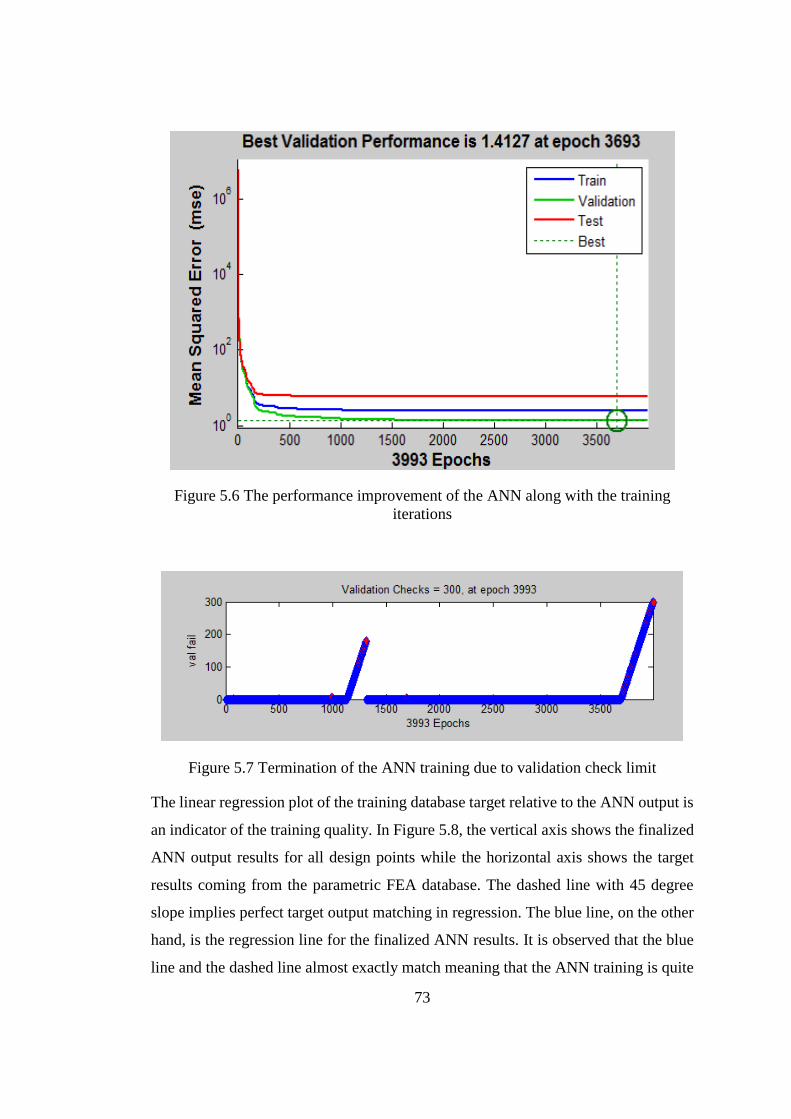
73

Figure 5.6 The performance improvement of the ANN along with the training

iterations

Figure 5.7 Termination of the ANN training due to validation check limit

The linear regression plot of the training database target relative to the ANN output is

an indicator of the training quality. In Figure 5.8, the vertical axis shows the finalized

ANN output results for all design points while the horizontal axis shows the target

results coming from the parametric FEA database. The dashed line with 45 degree

slope implies perfect target output matching in regression. The blue line, on the other

hand, is the regression line for the finalized ANN results. It is observed that the blue

line and the dashed line almost exactly match meaning that the ANN training is quite

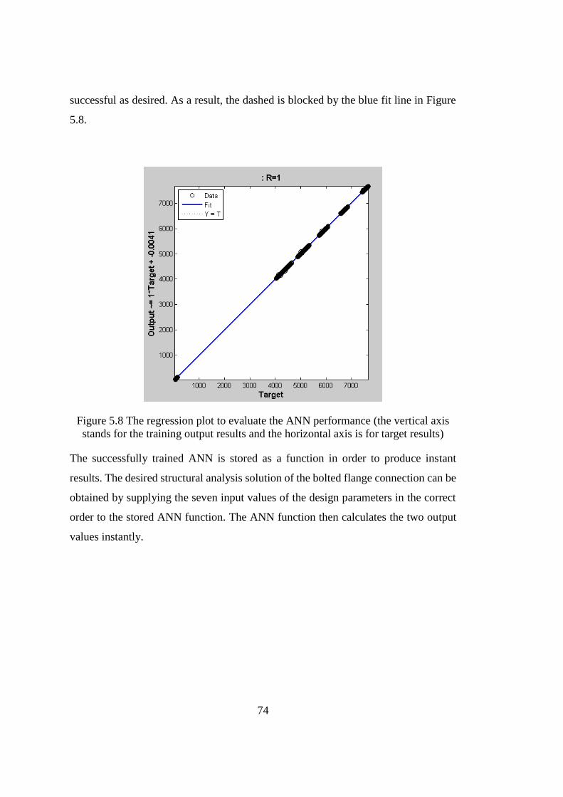
74

successful as desired. As a result, the dashed is blocked by the blue fit line in Figure

5.8.

Figure 5.8 The regression plot to evaluate the ANN performance (the vertical axis

stands for the training output results and the horizontal axis is for target results)

The successfully trained ANN is stored as a function in order to produce instant

results. The desired structural analysis solution of the bolted flange connection can be

obtained by supplying the seven input values of the design parameters in the correct

order to the stored ANN function. The ANN function then calculates the two output

values instantly.

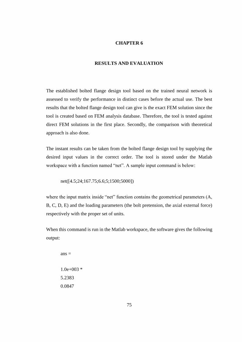
75

CHAPTER 6

RESULTS AND EVALUATION

The established bolted flange design tool based on the trained neural network is

assessed to verify the performance in distinct cases before the actual use. The best

results that the bolted flange design tool can give is the exact FEM solution since the

tool is created based on FEM analysis database. Therefore, the tool is tested against

direct FEM solutions in the first place. Secondly, the comparison with theoretical

approach is also done.

The instant results can be taken from the bolted flange design tool by supplying the

desired input values in the correct order. The tool is stored under the Matlab

workspace with a function named “net”. A sample input command is below:

net([4.5;24;167.75;6.6;5;1500;5000])

where the input matrix inside “net” function contains the geometrical parameters (A,

B, C, D, E) and the loading parameters (the bolt pretension, the axial external force)

respectively with the proper set of units.

When this command is run in the Matlab workspace, the software gives the following

output:

ans =

1.0e+003 *

5.2383

0.0847

76

where the 5238.3 is the bolt reaction force in N and 84.7 is the equivalent Von Mises

flange stress in MPa.

6.1 Comparison with Finite Element Analysis

The trained network has already been tested in the end of the training operation

automatically by Matlab [8]; however, the tool can be tested against direct FEM

solutions to check the accuracy of the approximation for different cases.

The test analyses are examined in three categories. The first set contains ten design

points selected randomly from the training points. Table 6.1 presents the ten test points

with the values of the parameters.

Table 6.1 Test set-1, (the samples are selected from the training points)

A, mm B, pcs C, mm D, mm E, mm

Axial

Force per

Bolt, N

Bolt

Pretension

, N

1 4.20 25.00 166.70 7.30 5.50 1152.00 5702.00

2 4.20 23.00 167.75 6.60 4.50 1024.00 4846.50

3 4.83 24.00 168.90 6.60 5.00 1408.00 4846.50

4 5.00 24.00 165.60 5.90 4.50 1280.00 6557.50

5 4.20 24.00 164.50 5.90 4.50 1152.00 3991.00

6 5.00 23.00 164.50 5.90 5.50 1280.00 7413.00

7 5.00 25.00 165.60 6.60 5.50 1280.00 3991.00

8 4.20 23.00 165.60 5.90 4.50 1024.00 3991.00

9 4.00 23.00 166.70 6.60 5.00 1408.00 3991.00

10 4.00 25.00 165.60 7.30 5.00 1536.00 7413.00

The ANN results for set-1 are given in Table 6.2. Table 6.2 shows that the bolted

flange design tool is able to give very accurate output values when the input values

are selected from the training points. If the FEM analysis output is taken as the correct

value, then the maximum percent error for the bolt force reaction is %0.040 while the

maximum absolute error is %1.5 for the average flange stress.

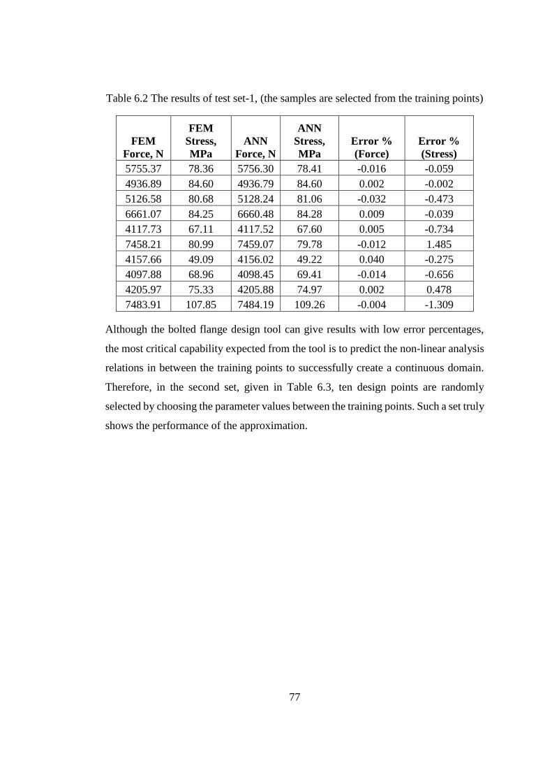
77

Table 6.2 The results of test set-1, (the samples are selected from the training points)

FEM

Force, N

FEM

Stress,

MPa

ANN

Force, N

ANN

Stress,

MPa

Error %

(Force)

Error %

(Stress)

5755.37 78.36 5756.30 78.41 -0.016 -0.059

4936.89 84.60 4936.79 84.60 0.002 -0.002

5126.58 80.68 5128.24 81.06 -0.032 -0.473

6661.07 84.25 6660.48 84.28 0.009 -0.039

4117.73 67.11 4117.52 67.60 0.005 -0.734

7458.21 80.99 7459.07 79.78 -0.012 1.485

4157.66 49.09 4156.02 49.22 0.040 -0.275

4097.88 68.96 4098.45 69.41 -0.014 -0.656

4205.97 75.33 4205.88 74.97 0.002 0.478

7483.91 107.85 7484.19 109.26 -0.004 -1.309

Although the bolted flange design tool can give results with low error percentages,

the most critical capability expected from the tool is to predict the non-linear analysis

relations in between the training points to successfully create a continuous domain.

Therefore, in the second set, given in Table 6.3, ten design points are randomly

selected by choosing the parameter values between the training points. Such a set truly

shows the performance of the approximation.

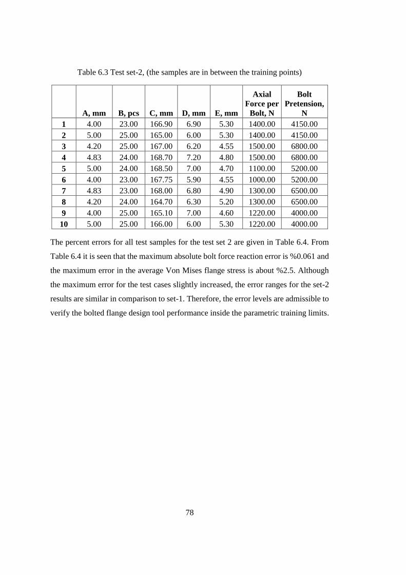
78

Table 6.3 Test set-2, (the samples are in between the training points)


Axial

Force per

Bolt, N

Bolt

Pretension,

N

1 4.00 23.00 166.90 6.90 5.30 1400.00 4150.00

2 5.00 25.00 165.00 6.00 5.30 1400.00 4150.00

3 4.20 25.00 167.00 6.20 4.55 1500.00 6800.00

4 4.83 24.00 168.70 7.20 4.80 1500.00 6800.00

5 5.00 24.00 168.50 7.00 4.70 1100.00 5200.00

6 4.00 23.00 167.75 5.90 4.55 1000.00 5200.00

7 4.83 23.00 168.00 6.80 4.90 1300.00 6500.00

8 4.20 24.00 164.70 6.30 5.20 1300.00 6500.00

9 4.00 25.00 165.10 7.00 4.60 1220.00 4000.00

10 5.00 25.00 166.00 6.00 5.30 1220.00 4000.00

The percent errors for all test samples for the test set 2 are given in Table 6.4. From

Table 6.4 it is seen that the maximum absolute bolt force reaction error is %0.061 and

the maximum error in the average Von Mises flange stress is about %2.5. Although

the maximum error for the test cases slightly increased, the error ranges for the set-2

results are similar in comparison to set-1. Therefore, the error levels are admissible to

verify the bolted flange design tool performance inside the parametric training limits.

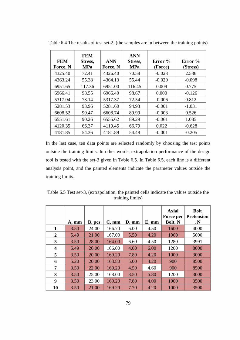
79

Table 6.4 The results of test set-2, (the samples are in between the training points)

FEM

Force, N

FEM

Stress,

MPa

ANN

Force, N

ANN

Stress,

MPa

Error %

(Force)

Error %

(Stress)

4325.40 72.41 4326.40 70.58 -0.023 2.536

4363.24 55.38 4364.13 55.44 -0.020 -0.098

6951.65 117.36 6951.00 116.45 0.009 0.775

6966.41 98.55 6966.40 98.67 0.000 -0.126

5317.04 73.14 5317.37 72.54 -0.006 0.812

5281.53 93.96 5281.60 94.93 -0.001 -1.031

6608.52 90.47 6608.74 89.99 -0.003 0.526

6551.61 90.26 6555.62 89.29 -0.061 1.085

4120.35 66.37 4119.45 66.79 0.022 -0.628

4181.85 54.36 4181.89 54.48 -0.001 -0.205

In the last case, ten data points are selected randomly by choosing the test points

outside the training limits. In other words, extrapolation performance of the design

tool is tested with the set-3 given in Table 6.5. In Table 6.5, each line is a different

analysis point, and the painted elements indicate the parameter values outside the

training limits.

Table 6.5 Test set-3, (extrapolation, the painted cells indicate the values outside the

training limits)


Axial

Force per

Bolt, N

Bolt

Pretension

, N

1 3.50 24.00 166.70 6.00 4.50 1600 4000

2 5.49 21.00 167.00 5.50 4.20 1000 5000

3 3.50 28.00 164.00 6.60 4.50 1280 3991

4 5.49 26.00 166.00 4.00 6.00 1200 8000

5 3.50 20.00 169.20 7.80 4.20 1000 3000

6 5.20 20.00 163.80 5.00 4.20 900 8500

7 3.50 22.00 169.20 4.50 4.60 900 8500

8 3.50 25.00 168.00 8.50 5.80 1200 3000

9 3.50 23.00 169.20 7.80 4.00 1000 3500

10 3.50 21.00 169.20 7.70 4.20 1000 3500

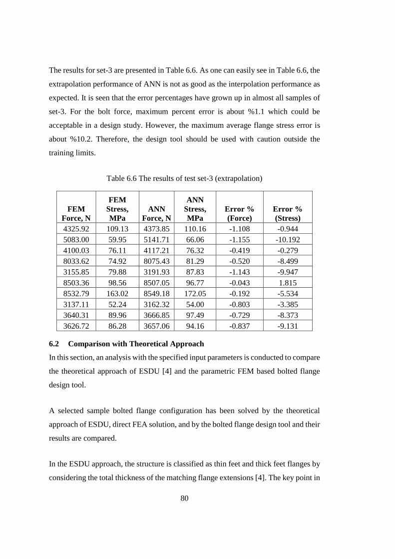
80

The results for set-3 are presented in Table 6.6. As one can easily see in Table 6.6, the

extrapolation performance of ANN is not as good as the interpolation performance as

expected. It is seen that the error percentages have grown up in almost all samples of

set-3. For the bolt force, maximum percent error is about %1.1 which could be

acceptable in a design study. However, the maximum average flange stress error is

about %10.2. Therefore, the design tool should be used with caution outside the

training limits.

Table 6.6 The results of test set-3 (extrapolation)

FEM

Force, N

FEM

Stress,

MPa

ANN

Force, N

ANN

Stress,

MPa

Error %

(Force)

Error %

(Stress)

4325.92 109.13 4373.85 110.16 -1.108 -0.944

5083.00 59.95 5141.71 66.06 -1.155 -10.192

4100.03 76.11 4117.21 76.32 -0.419 -0.279

8033.62 74.92 8075.43 81.29 -0.520 -8.499

3155.85 79.88 3191.93 87.83 -1.143 -9.947

8503.36 98.56 8507.05 96.77 -0.043 1.815

8532.79 163.02 8549.18 172.05 -0.192 -5.534

3137.11 52.24 3162.32 54.00 -0.803 -3.385

3640.31 89.96 3666.85 97.49 -0.729 -8.373

3626.72 86.28 3657.06 94.16 -0.837 -9.131

6.2 Comparison with Theoretical Approach

In this section, an analysis with the specified input parameters is conducted to compare

the theoretical approach of ESDU [4] and the parametric FEM based bolted flange

design tool.

A selected sample bolted flange configuration has been solved by the theoretical

approach of ESDU, direct FEA solution, and by the bolted flange design tool and their

results are compared.

In the ESDU approach, the structure is classified as thin feet and thick feet flanges by

considering the total thickness of the matching flange extensions [4]. The key point in

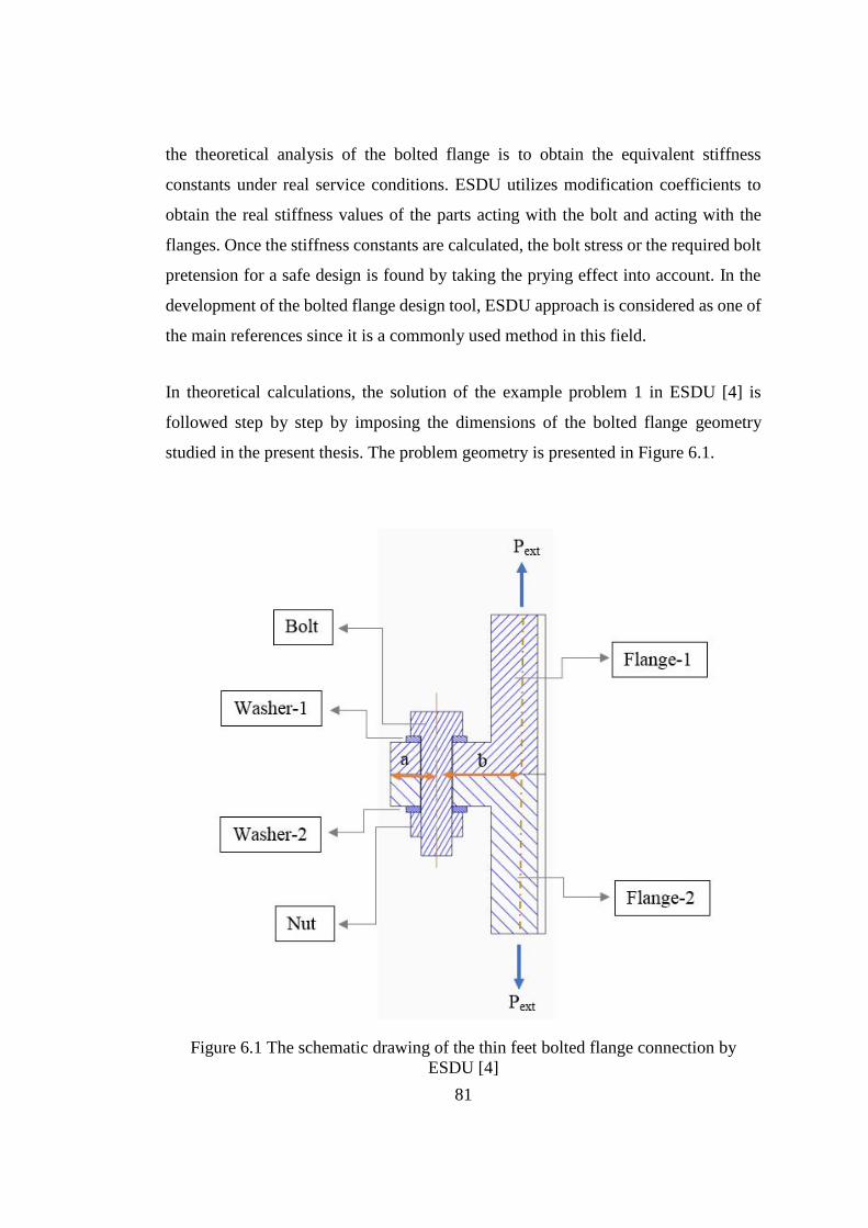
81

the theoretical analysis of the bolted flange is to obtain the equivalent stiffness

constants under real service conditions. ESDU utilizes modification coefficients to

obtain the real stiffness values of the parts acting with the bolt and acting with the

flanges. Once the stiffness constants are calculated, the bolt stress or the required bolt

pretension for a safe design is found by taking the prying effect into account. In the

development of the bolted flange design tool, ESDU approach is considered as one of

the main references since it is a commonly used method in this field.

In theoretical calculations, the solution of the example problem 1 in ESDU [4] is

followed step by step by imposing the dimensions of the bolted flange geometry

studied in the present thesis. The problem geometry is presented in Figure 6.1.

Figure 6.1 The schematic drawing of the thin feet bolted flange connection by

ESDU [4]

82

The details of the new bolted flange joint are:

• 𝐴(𝑏𝑜𝑙𝑡 𝑠𝑖𝑧𝑒) = 𝑀4 (4 𝑚𝑚)

• 𝐵 (𝑡ℎ𝑒 𝑛𝑢𝑚𝑏𝑒𝑟 𝑜𝑓 𝑏𝑜𝑙𝑡𝑠) = 24 (𝑛𝑜𝑡 𝑎𝑝𝑝𝑙𝑖𝑐𝑎𝑏𝑙𝑒 ℎ𝑒𝑟𝑒)

• 𝐶 (𝑏𝑜𝑙𝑡 𝑙𝑜𝑐𝑎𝑡𝑖𝑜𝑛) = 167.75 𝑚𝑚

• 𝐷 (𝑐𝑎𝑠𝑖𝑛𝑔 𝑡ℎ𝑖𝑐𝑘𝑛𝑒𝑠𝑠𝑒𝑠) = 6.6 𝑚𝑚

• 𝐸(𝑓𝑙𝑎𝑛𝑔𝑒 𝑡ℎ𝑖𝑐𝑘𝑛𝑒𝑠𝑠𝑒𝑠) = 5 𝑚𝑚

• 𝑡𝑏ℎ (𝑏𝑜𝑙𝑡 ℎ𝑒𝑎𝑑 𝑎𝑛𝑑 𝑛𝑢𝑡 𝑡ℎ𝑖𝑐𝑘𝑛𝑒𝑠𝑠𝑒𝑠) = 3.2 𝑚𝑚

• 𝑝(𝑝𝑖𝑡𝑐ℎ 𝑜𝑓 𝑡ℎ𝑒 𝑏𝑜𝑙𝑡 𝑡ℎ𝑟𝑒𝑎𝑑) = 0.7 𝑚𝑚

• 𝑑𝑚𝑖𝑛 (𝑏𝑜𝑙𝑡 𝑡ℎ𝑟𝑒𝑎𝑑 𝑚𝑖𝑛𝑜𝑟 𝑑𝑖𝑎𝑚𝑒𝑡𝑒𝑟) = 3.2 𝑚𝑚

• 𝑃𝑡 (𝐵𝑜𝑙𝑡 𝑝𝑟𝑒𝑡𝑒𝑛𝑠𝑖𝑜𝑛) = 4000 𝑁

• 𝑃𝑒𝑥𝑡 (𝐴𝑥𝑖𝑎𝑙 𝑒𝑥𝑡𝑒𝑟𝑛𝑎𝑙 𝑓𝑜𝑟𝑐𝑒) = 1500 𝑁

• 𝑡𝑤 (𝑤𝑎𝑠ℎ𝑒𝑟 𝑡ℎ𝑖𝑐𝑘𝑛𝑒𝑠𝑠) = 0.8 𝑚𝑚

• 𝑑𝑤 (𝑤𝑎𝑠ℎ𝑒𝑟 𝑜𝑢𝑡𝑒𝑟 𝑑𝑖𝑎𝑚𝑒𝑡𝑒𝑟) = 8 𝑚𝑚

• 𝑑𝑤𝑖 (𝑤𝑎𝑠ℎ𝑒𝑟 𝑎𝑛𝑑 𝑓𝑙𝑎𝑛𝑔𝑒 𝑖𝑛𝑛𝑒𝑟 (ℎ𝑜𝑙𝑒) 𝑑𝑖𝑎𝑚𝑒𝑡𝑒𝑟) = 4.4 𝑚𝑚

• 𝑑𝑏ℎ (𝑏𝑜𝑙𝑡 ℎ𝑒𝑎𝑑 𝑒𝑓𝑓𝑒𝑐𝑡𝑖𝑣𝑒 𝑑𝑖𝑎𝑚𝑒𝑡𝑒𝑟) = 6.8 𝑚𝑚

• 𝑅𝑜𝑢𝑡 (𝑓𝑙𝑎𝑛𝑔𝑒 𝑜𝑢𝑡𝑒𝑟 𝑟𝑎𝑑𝑖𝑢𝑠) = 175 𝑚𝑚

• 𝑅𝑖𝑛 (𝑓𝑙𝑎𝑛𝑔𝑒 𝑖𝑛𝑛𝑒𝑟 𝑟𝑎𝑑𝑖𝑢𝑠) = 151.9 𝑚𝑚

• 𝐸𝑏 (𝑌𝑜𝑢𝑛𝑔’𝑠 𝑚𝑜𝑑𝑢𝑙𝑢𝑠 𝑜𝑓 𝑏𝑜𝑙𝑡) = 200 𝐺𝑃𝑎

• 𝐸𝑓 (𝑌𝑜𝑢𝑛𝑔’𝑠 𝑚𝑜𝑑𝑢𝑙𝑢𝑠 𝑜𝑓 𝑓𝑙𝑎𝑛𝑔𝑒𝑠) = 71 𝐺𝑃𝑎

• 𝐸𝑤 (𝑌𝑜𝑢𝑛𝑔’𝑠 𝑚𝑜𝑑𝑢𝑙𝑢𝑠 𝑜𝑓 𝑤𝑎𝑠ℎ𝑒𝑟𝑠) = 200 𝐺𝑃𝑎

• 𝑎 (𝑡ℎ𝑒 𝑑𝑖𝑠𝑡𝑎𝑛𝑐𝑒 𝑓𝑟𝑜𝑚 𝑏𝑜𝑙𝑡 𝑐𝑒𝑛𝑡𝑒𝑟 𝑡𝑜 𝑜𝑢𝑡𝑒𝑟 𝑓𝑙𝑎𝑛𝑔𝑒 𝑠𝑢𝑟𝑓𝑎𝑐𝑒) =

7.25 𝑚𝑚

• 𝑏 (𝑡ℎ𝑒 𝑑𝑖𝑠𝑡𝑎𝑛𝑐𝑒 𝑓𝑟𝑜𝑚 𝑏𝑜𝑙𝑡 𝑐𝑒𝑛𝑡𝑒𝑟 𝑡𝑜 𝑖𝑛𝑛𝑒𝑟 𝑓𝑙𝑎𝑛𝑔𝑒 𝑠𝑢𝑟𝑓𝑎𝑐𝑒) =

12.55 𝑚𝑚

The ESDU calculation steps [4] can be followed step by step below. The process starts

with the calculation of equivalent stiffness of the bolt group according to Equation

6.1. The bolt group stiffness is formed by the effective bolt thread stiffness (𝑘𝑡ℎ),

effective bolt shank stiffness (𝑘𝑠ℎ), the washers’ stiffness (𝑘𝑤), the stiffness of the

flange-1 acting with the bolt group (𝑘𝑓𝑏1), and the stiffness of the flange-2 acting with

the bolt group (𝑘𝑓𝑏2). A portion of the flange pair thicknesses are assumed to act with

83

the bolt group since the external force is transferred to bolt group through these

regions. The flange located close to bolt head is named as flange-1 and the flange

closer to the nut is called as flange-2. ESDU suggests to assume that ¼ thickness of

the total flange-1 thickness acts with the bolt group and the remaining ¾ of the flange-

1 thickness acts with the flange group while calculating the effective stiffness values.

In the same way, the stiffness contributions to bolt group by flange-2 is taken as 1/5

of the total flange-2 thickness based on the experience of ESDU.

(𝑘𝑏′ )−1 = (𝑘𝑡ℎ)−1 + (𝑘𝑠ℎ)−1 + (𝑘𝑤)−1 + (𝑘𝑓𝑏1)

−1+ (𝑘𝑓𝑏2)−1 (6.1)

The shank portion of the bolt is equal to the sum of the thicknesses of the flanges and

the washers:

𝑙𝑠ℎ = 2 ∙ 𝐸 + 2 ∙ 𝑡𝑤 (6.2)

𝑙𝑠ℎ = 11.6 𝑚𝑚 (6.3)

A portion of the flexible bolt head acts as part of the shank. Therefore, the effective

bolt shank length (𝑙𝑠ℎ′ ) is calculated as given in Equation 6.4. This effect is represented

by the shank increase coefficient (𝑥𝑠ℎ). The coefficient is taken as 0.2 as suggested by

ESDU [4].

𝑙𝑠ℎ′ = 𝑙𝑠ℎ + 𝑥𝑠ℎ ∙ 𝑡𝑏ℎ (6.4)

𝑙′𝑠ℎ = 12.24 𝑚𝑚 (6.5)

The effective bolt shank stiffness is calculated with the cross-sectional area of the

shank by considering Equation 6.6:

𝑘𝑠ℎ = 𝐸𝑏 ∙ (𝜋 ∙ 𝐴2/4)/𝑙′𝑠ℎ (6.6)

𝑘𝑠ℎ = 205.333 ∙ 106 𝑁/𝑚 (6.7)

84

In order to calculate the stiffness of the threaded section of the bolt, the effective

length of the threaded portion of the bolt is calculated first. Since the threaded portion

of the bolt is assumed to begin with the nut engagement, the threaded portion length

inside the flange hole is taken as zero so 𝑙𝑡ℎ is “0” in Equation 6.8. The stiffness

contribution by the bolt thread inside the nut is considered with the thread engagement

coefficient (𝑥𝑝𝑡) by multiplying it with the thread pitch (𝑝) in Equation 6.8. The third

term on right hand side in Equation 6.8 represents the effective length term of the nut

contributing to the stiffness of the threaded portion via the nut coefficient (𝑥𝑛𝑢).

ESDU [4] suggests 𝑥𝑝𝑡to be taken as 1 and 𝑥𝑛𝑢 to be taken as 2 for the standard nut.

𝑙𝑡ℎ′ = 𝑙𝑡ℎ + 𝑥𝑝𝑡 ∙ 𝑝 + 𝑥𝑛𝑢 ∙ 𝐴 (6.8)

𝑙𝑡ℎ′ = 8.7 𝑚𝑚 (6.9)

The effective diameter of the threaded portion of the bolt (𝑑𝑡ℎ′ ) is also needed and it

is calculated by taking an average value between the minimum diameter of the

threaded portion of the bolt (𝑑𝑚𝑖𝑛) and the nominal bolt diameter (𝐴) with the typical

thread diameter coefficient (𝑥𝑡ℎ) of 0.3 multiplying the difference as suggested by

ESDU [4].

𝑑𝑡ℎ′ = 𝑑𝑚𝑖𝑛 + 𝑥𝑡ℎ ∙ (𝐴 − 𝑑𝑚𝑖𝑛) (6.10)

𝑑𝑡ℎ′ = 3.44 𝑚𝑚 (6.11)

The effective stiffness of the threaded portion of the bolt is calculated by Equation

6.12:

𝑘𝑡ℎ = 𝐸𝑏 ∙ (𝜋 ∙ 𝑑𝑡ℎ′ 2

/4)/𝑙′𝑡ℎ (6.12)

𝑘𝑡ℎ = 213.657 ∙ 106 𝑁/𝑚 (6.13)

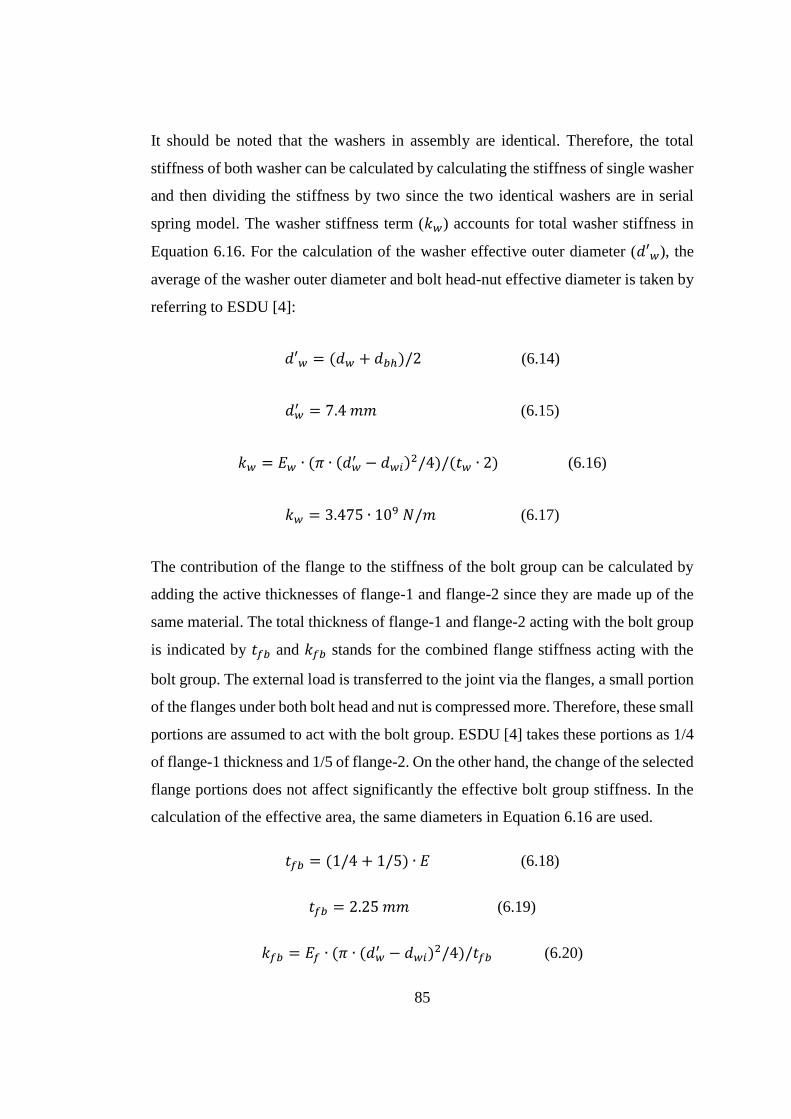
85

It should be noted that the washers in assembly are identical. Therefore, the total

stiffness of both washer can be calculated by calculating the stiffness of single washer

and then dividing the stiffness by two since the two identical washers are in serial

spring model. The washer stiffness term (𝑘𝑤) accounts for total washer stiffness in

Equation 6.16. For the calculation of the washer effective outer diameter (𝑑′𝑤), the

average of the washer outer diameter and bolt head-nut effective diameter is taken by

referring to ESDU [4]:

𝑑′𝑤 = (𝑑𝑤 + 𝑑𝑏ℎ)/2 (6.14)

𝑑𝑤′ = 7.4 𝑚𝑚 (6.15)

𝑘𝑤 = 𝐸𝑤 ∙ (𝜋 ∙ (𝑑𝑤′ − 𝑑𝑤𝑖)

2/4)/(𝑡𝑤 ∙ 2) (6.16)

𝑘𝑤 = 3.475 ∙ 109 𝑁/𝑚 (6.17)

The contribution of the flange to the stiffness of the bolt group can be calculated by

adding the active thicknesses of flange-1 and flange-2 since they are made up of the

same material. The total thickness of flange-1 and flange-2 acting with the bolt group

is indicated by 𝑡𝑓𝑏 and 𝑘𝑓𝑏 stands for the combined flange stiffness acting with the

bolt group. The external load is transferred to the joint via the flanges, a small portion

of the flanges under both bolt head and nut is compressed more. Therefore, these small

portions are assumed to act with the bolt group. ESDU [4] takes these portions as 1/4

of flange-1 thickness and 1/5 of flange-2. On the other hand, the change of the selected

flange portions does not affect significantly the effective bolt group stiffness. In the

calculation of the effective area, the same diameters in Equation 6.16 are used.

𝑡𝑓𝑏 = (1/4 + 1/5) ∙ 𝐸 (6.18)

𝑡𝑓𝑏 = 2.25 𝑚𝑚 (6.19)

𝑘𝑓𝑏 = 𝐸𝑓 ∙ (𝜋 ∙ (𝑑𝑤′ − 𝑑𝑤𝑖)

2/4)/𝑡𝑓𝑏 (6.20)

86

𝑘𝑓𝑏 = 1.837 ∙ 109 𝑁/𝑚 (6.21)

The effective bolt stiffness is now calculated by Equation 6.1.

𝑘𝑏′ = 96.314 ∙ 106

𝑁

𝑚 (6.22)

In order to calculate the effective flange stiffness, it is critical to determine the

effective contact area. For this purpose, ESDU [4] offers a chart to determine the

effective area of the flanges. To utilize the chart, two different ratios are calculated in

Equations 6.27 and 6.28. 𝑙′𝑓 is the equivalent flange thickness given by Equation 6.23

including the washer thicknesses.

𝑙′𝑓 = 2 ∙ (𝐸 + 𝑡𝑤) (6.23)

𝑙′𝑓 = 11.6 𝑚𝑚 (6.24)

The effective diameter of the practical working area can be calculated in a few

different ways. As suggested by ESDU [4], twice the distance from the bolt center to

the outer end of the flange is used here.

𝐷𝑓 = 2 ∙ (𝑅𝑜𝑢𝑡 − 𝐶) (6.25)

𝐷𝑓 = 14.5 mm (6.26)

Now, we can determine the ratios to use the chart and by using these ratios the

equation for the effective flange area is calculated by Equation 6.29 with the constant

value 1.27 read from the chart. The chart can be seen in Appendix C.

𝐷𝑓/𝑑′𝑤 = 1.959 (6.27)

𝑙′𝑓/𝑑′𝑤 = 1.568 (6.28)

87

𝐴𝑓

(𝜋4) ∙ ((𝑑′

𝑤)2 − (𝑑𝑤𝑖)2)= 1.27 (6.29)

𝐴𝑓 = 3.531 ∙ 10−5𝑚2 (6.30)

The effective flange stiffness, 𝑘′𝑓, is calculated by Equation 6.31 and the numerical

result is in Equation 6.32.

𝑘′𝑓 = 𝐸𝑓 ∙ (𝐴𝑓)/((3

4+

4

5) ∙ 𝐸) (6.31)

𝑘′𝑓 = 323.485𝑥106 𝑁/𝑚 (6.32)

To summarize, by following each calculation step in the ESDU example [4], and

taking the same modification coefficients, equivalent stiffness of the bolt group (the

structure acting with bolt) and the equivalent stiffness of the flange group (the

structure acting with two flanges) are found as:

• 𝑘𝑏′ = 96.314𝑥106 𝑁/𝑚

• 𝑘𝑓′ = 323.485𝑥106 𝑁/𝑚

At this stage of the solution, the possibility of separation must be checked. In case of

separation, the prying effect drastically increase the load carried by the bolt group. 𝑃𝑎𝑠

is the critical externally applied load to separate the flanges from each other. 𝑃𝑎𝑠 value

can be calculated by Equation 6.33. In case of separation, the bolt load including

prying effect has to exceed 𝑃𝑎𝑠. Separation control can be made by calculating the

bolt load with prying effect in Equation 6.35. As specified above, the distance from

bolt center to outer flange surface (a) is 7.25 mm and the distance from bolt center to

flange inner surface (b) is 12.35 mm.

𝑃𝑎𝑠 = 𝑃𝑡 ∙𝑘′

𝑏 + 𝑘′𝑓

𝑘′𝑓

(6.33)

88

𝑃𝑎𝑠 = 5190.95 𝑁 (6.34)

𝑃𝑏 = 𝑃𝑒𝑥𝑡 ∙ (1 +𝑏

𝑎) (6.35)

𝑃𝑏 = 4096.55 𝑁 (6.36)

As seen in Equation 6.36, the bolt load with prying effect is less than the critical value

for separation. As a result, the load carried by the bolt group is calculated without

considering the prying effect. The portion of the external load carried by the bolt is

calculated by considering the stiffness ratio of the bolt and the flange groups. 𝑃𝑡 is

bolt pretension value in Equation 6.36. The bolt load is calculated as:

𝑃𝑏 = 𝑃𝑡 + 𝑃𝑒𝑥𝑡 ∙𝑘′

𝑏

𝑘′𝑓 + 𝑘′

𝑏

(6.37)

𝑃𝑏 = 4344.14 𝑁 (6.38)

The same problem is modeled in ANSYS and finite element analysis of the bolted

flange connection involving contact is performed. The bolt force reaction is obtained

as 4306.4 N as seen in Figure 6.2.

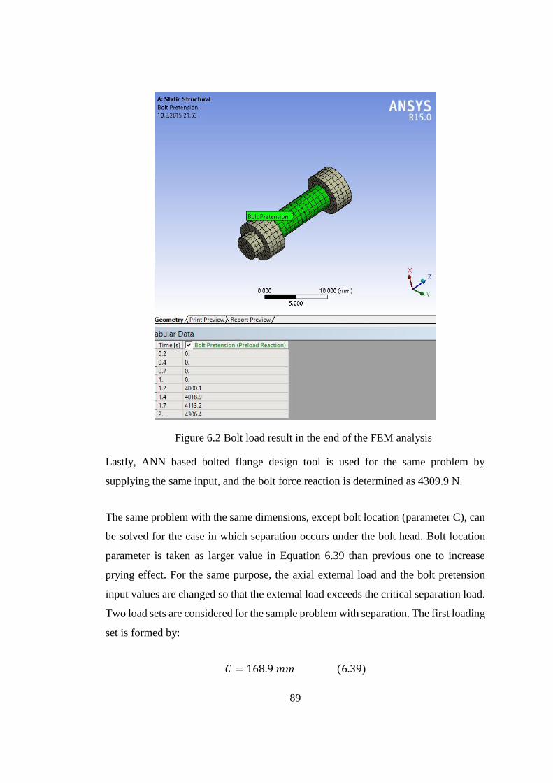
89

Figure 6.2 Bolt load result in the end of the FEM analysis

Lastly, ANN based bolted flange design tool is used for the same problem by

supplying the same input, and the bolt force reaction is determined as 4309.9 N.

The same problem with the same dimensions, except bolt location (parameter C), can

be solved for the case in which separation occurs under the bolt head. Bolt location

parameter is taken as larger value in Equation 6.39 than previous one to increase

prying effect. For the same purpose, the axial external load and the bolt pretension

input values are changed so that the external load exceeds the critical separation load.

Two load sets are considered for the sample problem with separation. The first loading

set is formed by:

𝐶 = 168.9 𝑚𝑚 (6.39)

90

𝑃𝑡 = 1000 𝑁 (6.40)

𝑃𝑒𝑥𝑡 = 1500 𝑁 (6.41)

The stiffness values are the same for both groups as before. Therefore, the critical

separation load is calculated in Equation 6.42 with the same stiffness values as in

Equation 6.33.

𝑃𝑎𝑠 = 1297.7 𝑁 (6.42)

Due to having larger external force than the critical load, the separation under bolt

head is assumed. “a” and “b” values are calculated again with respect to new “C”

value in Equations 6.43 and 6.44.

𝑎 = 𝑅𝑜𝑢𝑡 − 𝐶 (6.43)

𝑏 = 𝐶 − 𝑅𝑖𝑛 − 𝐷/2 (6.44)

𝑎 = 6.1 𝑚𝑚 (6.45)

𝑏 = 13.7 𝑚𝑚 (6.46)

The bolt reaction force is now calculated by considering the separation with Equation

6.35.

𝑃𝑏 = 4868.9 𝑁 (6.47)

However, FEM solution gives the bolt reaction force of 2789.8 N and the developed

bolted flange design tool gives 2332.7 N for the same problem.

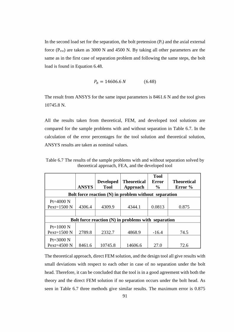
91

In the second load set for the separation, the bolt pretension (Pt) and the axial external

force (Pext) are taken as 3000 N and 4500 N. By taking all other parameters are the

same as in the first case of separation problem and following the same steps, the bolt

load is found in Equation 6.48.

𝑃𝑏 = 14606.6 𝑁 (6.48)

The result from ANSYS for the same input parameters is 8461.6 N and the tool gives

10745.8 N.

All the results taken from theoretical, FEM, and developed tool solutions are

compared for the sample problems with and without separation in Table 6.7. In the

calculation of the error percentages for the tool solution and theoretical solution,

ANSYS results are taken as nominal values.

Table 6.7 The results of the sample problems with and without separation solved by

theoretical approach, FEA, and the developed tool

ANSYS

Developed

Tool

Theoretical

Approach

Tool

Error

%

Theoretical

Error %

Bolt force reaction (N) in problem without separation

Pt=4000 N

Pext=1500 N 4306.4 4309.9 4344.1 0.0813 0.875

Bolt force reaction (N) in problems with separation

Pt=1000 N

Pext=1500 N 2789.8 2332.7 4868.9 -16.4 74.5

Pt=3000 N

Pext=4500 N 8461.6 10745.8 14606.6 27.0 72.6

The theoretical approach, direct FEM solution, and the design tool all give results with

small deviations with respect to each other in case of no separation under the bolt

head. Therefore, it can be concluded that the tool is in a good agreement with both the

theory and the direct FEM solution if no separation occurs under the bolt head. As

seen in Table 6.7 three methods give similar results. The maximum error is 0.875

92

percent by the theoretical approach result. On the other hand, the solutions obtained

from theoretical method are too different than the solutions from the others for the

sample problems with separation. One should realize that developed bolted flange

design tool extrapolates the results in the separation problems since the bolt pretension

in the first case and the axial external force in the second case are out of ANN training

limits. Nevertheless, theoretical approach results far worse than the tool results with

74.5 % and 72.6 % deviations in separation problems. As a results, developed bolted

flange design tool exhibits better performance than theoretical method in overall

evaluation.

93

CHAPTER 7

CONCLUSION AND FUTURE WORKS

7.1 Conclusion

In this study, an ANN based bolted flange design tool is developed. ANN based

design tool is established utilizing the non-linear finite element analysis database with

contact and frictional nonlinearities. The tool is designed for the design and analysis

of the bolted flange connection of a medium scale aircraft engine under axial load.

Since the developed tool utilizes artificial neural network approximation of the

database formed by non-linear finite element analysis involving contact, the structural

analysis of the bolted flange joint can be made very fast with high accuracy with the

developed tool.

The development procedure of the ANN based design tool requires the determination

of input parameters to be used in parametric analysis. The geometric variables used in

the design tool are defined to be the bolt size, the number of bolts, bolt location, casing

thickness, and flange thickness with upper and lower limit input limits while the load

variables are the axial external force and the bolt pretension. Parameters correlation

study is conducted to determine the sensitivities of the input parameters on the output

and to decide on the number of intervals for each variable in the upper and the lower

range of the design variables. For the training of the ANN, a parametric study with

13500 non-linear FE analyses is conducted to form a FEA solution database. The FEA

database comprises the combination of all input parameter values with each other. In

the final step, the created FEA database is trained to setup an artificial neural network

to establish the bolted flange design tool. ANN based design tool gives two output.

The first one is the force reaction in the bolt body and the second one is the average

Von Mises stress in the flange. The trained ANN based bolted flange design tool gives

94

parametric analysis results instantly within a continuous input domain within the

upper and lower limits of each design variable.

The developed bolted flange design tool is verified via two case studies. In the first

one, the tool is tested against the commercial FEA software for three separate

conditions: the test points the same with the training points, the test points between

the training points (interpolation), and the test points outside the limits of training

points (extrapolation). The analysis results show that the tool delivers successful

results with very low deviation from the direct FEA solutions when the test points are

within the training limits. When the test points are outside the limits of the training

points, the performance of the tool drops, as expected. However, in the overall, the

ANN based bolted flange design tool performs very well in approximating the non-

linear behavior of the bolted flange analysis results obtained by FEM. Utilization of

the tool eliminates time requirements in FEA.

In the second case study the bolted flange design tool output is compared with the

results of the theoretical approach [4] for the same problems of the cases with and

without separation. The results showed that the theoretical approach and the bolted

flange design tool are consistent with each other for the bolt reaction force until the

separation of flange. As both case studies suggest, the developed ANN based bolted

flange design tool can be used as a reliable structural analysis method inside the

training domain. On the other hand, theoretical approach gives too inaccurate results

in comparison to FEM solution when the separation under the bolt head occurs.

Although the developed tool is tested with extrapolation outside the training limits, it

gives closer results to FEM results when compared with the theoretical results in

separation problem. If the tool is trained further for larger limits including the input

parameters causing separation, it can give quite reliable results as FEM solutions.

Therefore, theoretical approach has a limited applicability in structural analysis of

bolted flange connection. Moreover, ESDU approach focusses on the bolt force and

the bolt stress rather than flange stress. However, developed tool can give solution for

both bolt and flange in structural analysis by taking power of FEA.

95

It is also concluded that the ANN based flange design tool can be used as the fast

solver in conjunction with an optimizer to achieve weight reduction in the aircraft

engine flange. In the optimization process, ANN based design tool serves as very

accurate approximate model replacing the non-linear finite element solver. Thus, with

the ANN based solver, flange optimization can be performed very fast compared to

employing non-linear FE based solver in each design iteration in the optimization

process.

The study conducted here not only demonstrates the successful use of the ANN as the

bolted flange design tool, but also shows promise for the applicability of this

methodology to different non-linear structural problems.

7.2 Future Works

The study intends to offer a new approach to axisymmetric circular bolted flange

connections. The developed methodology is applied for the bolted flange connection

exposed to axial external force. However, this approach is not only limited with single

load condition but also any loading type or the combinations can be integrated into

the tool. Moreover, it is possible to broaden the scope of the tool by enlarging the

parametric input limits and increasing the number of the parameters. In order to

improve the extent and the abilities of the bolted flange connection tool, the finite

element analysis database can be systematically enriched by adding more analyses.

Obviously, the larger the training database, the better the artificial neural network. By

including different loading types and enlarging the input database, the developed tool

can be used for larger scope of bolted flange problems. Moreover, in the near future

a graphical user interface is going to be created for the ease of use of the bolted flange

design tool. The developed tool with a graphical user interface can be utilized as an

optimization tool to reduce bolted flange connection weight in design.

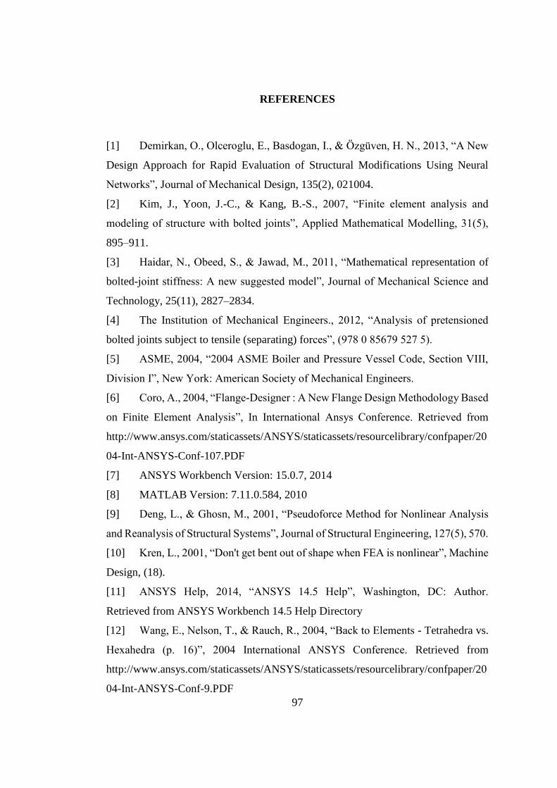
97

REFERENCES

[1] Demirkan, O., Olceroglu, E., Basdogan, I., & Özgüven, H. N., 2013, “A New

Design Approach for Rapid Evaluation of Structural Modifications Using Neural

Networks”, Journal of Mechanical Design, 135(2), 021004.

[2] Kim, J., Yoon, J.-C., & Kang, B.-S., 2007, “Finite element analysis and

modeling of structure with bolted joints”, Applied Mathematical Modelling, 31(5),

895–911.

[3] Haidar, N., Obeed, S., & Jawad, M., 2011, “Mathematical representation of

bolted-joint stiffness: A new suggested model”, Journal of Mechanical Science and

Technology, 25(11), 2827–2834.

[4] The Institution of Mechanical Engineers., 2012, “Analysis of pretensioned

bolted joints subject to tensile (separating) forces”, (978 0 85679 527 5).

[5] ASME, 2004, “2004 ASME Boiler and Pressure Vessel Code, Section VIII,

Division I”, New York: American Society of Mechanical Engineers.

[6] Coro, A., 2004, “Flange-Designer : A New Flange Design Methodology Based

on Finite Element Analysis”, In International Ansys Conference. Retrieved from

http://www.ansys.com/staticassets/ANSYS/staticassets/resourcelibrary/confpaper/20

04-Int-ANSYS-Conf-107.PDF

[7] ANSYS Workbench Version: 15.0.7, 2014

[8] MATLAB Version: 7.11.0.584, 2010

[9] Deng, L., & Ghosn, M., 2001, “Pseudoforce Method for Nonlinear Analysis

and Reanalysis of Structural Systems”, Journal of Structural Engineering, 127(5), 570.

[10] Kren, L., 2001, “Don't get bent out of shape when FEA is nonlinear”, Machine

Design, (18).

[11] ANSYS Help, 2014, “ANSYS 14.5 Help”, Washington, DC: Author.

Retrieved from ANSYS Workbench 14.5 Help Directory

[12] Wang, E., Nelson, T., & Rauch, R., 2004, “Back to Elements - Tetrahedra vs.

Hexahedra (p. 16)”, 2004 International ANSYS Conference. Retrieved from

http://www.ansys.com/staticassets/ANSYS/staticassets/resourcelibrary/confpaper/20

04-Int-ANSYS-Conf-9.PDF

98

[13] Zienkiewicz, O. C., & Morgan, K., 2006, “Finite Elements & Approximation”,

New York, NY: Dover Publications, Chap. 5.

[14] Cook, R. D., Malkus, D. S., Plesha, M. E., & Witt, R. J., 2001, “Concepts and

Applications of Finite Element Analysis”, Hoboken, NJ: John Wiley & Sons, Chap.

6.

[15] Cook, R. D., Malkus, D. S., Plesha, M. E., Witt, R. J., 2001, “Concepts and

Applications of Finite Element Analysis, 4th Edition”, Wiley. ISBN: 9780471356059

[16]] Heinstein, M.W., Attaway, S.W., Swegle, J.W., & Mello, F.J., 1993, “A

general-purpose contact detection algorithm for nonlinear structural analysis codes”,

New Mexico: Sandia National Laboratories. Print. SAND92-2141.

[17] “An Augmented Lagrangian Formulation for the Finite Element Solution of

Contact Problems”, 1986, California: University of California at Berkeley. Print. AD-

A166 649.

[18] Muliana, A., Steward, R., Haj-Ali, R. M. & Saxena, A., 2002, “Artificial

Neural Network and Finite Element Modeling of Nanoindentation Tests”,

Metallurgical and Materials Transactions A.

[19] Budynas, R. G., Nisbett, J. K., 2008, “Shigley’s Mechanical Engineering

Design (8th ed.)”, New York, NY: McGraw-Hill, Chap. 8.

[20] Schaaf, M., Bartonicek, J., 2003, “Calculation of Bolted Flange Connections

of Floating and Metal-To-Metal Contact Type”, Proceedings of PVP2003.

[21] Azim, R., 2013, “An Analytical Investigation On Bolt Tension Of A Flanged

Steel Pipe Joint Subjected to Bending Moments”, International Journal of Engineering

and Applied Sciences, 2(3), 71-81.

[22] MATLAB Help, 2010, “MATLAB 2010 Help”, DC: Author. Retrieved from

MATLAB 2010 Help Directory

[23] TEI, Inc. http://www.tei.com.tr

[24] Metric Fasteners (n.d.). Retrieved April 12, 2015, from

http://www.metrication.com/engineering/fastener.html

[25] Multistandard Components Corp., 2000, “Full Thread Hexagon Head

Screws”, Retrieved April 12, 2015, from http://www.metricmcc.com/catalog/ch1/1-

2.pdf

99

[26] “Reference Tables -- Coefficient of Friction”, 2015, April 4. Retrieved from

http://www.engineershandbook.com/Tables/frictioncoefficients.htm

[27] Microsoft Excel Version: 15.0.4701.1001, 2013.

[28] Suratgar, A. A., Tavakoli, M. B., & Hoseinabadi, A., 2007, "Modified

Levenberg-Marquardt Method for Neural Networks Training", International Journal

of Computer, Control, Quantum and Information Engineering, 1(6), 1719-1721.

[29] Graupe, D. (2013). “Principles of Artificial Neural Networks (3rd Edition)”.

Singapore: World Scientific Publishing Company

[30] Gomes, H. M., & Awruch, A. M., 2004, “Comparison of response surface and

neural network with other methods for structural reliability analysis”, Structural

Safety, 2649-67.

[31] Petrini, M., 2012, “Improvements to The Backpropagation Algorithm”,

Annals of The University of Petrosani Economics, 12(4), 185-192.

[32] Corder, G.W., & Foreman, D.I., 2014, “Nonparametric Statistics: A Step-by-

Step Approach”, Wiley, ISBN 978-1118840313

[33] Borkowf, C. B., 2000, “A new nonparametric method for variance estimation

and confidence interval construction for Spearman's rank correlation”, Computational

Statistics and Data Analysis, 34219-241.

[34] Wall Emerson, R., 2015, Causation and Pearson's Correlation Coefficient,

Journal of Visual Impairment & Blindness, 36(3), 242-244.

[35] Yildirim, A., Akay, A., Gulasik, H., Coker, D., Gurses, E., & Kayran, A.

(2015). Development of Bolted Flange Design Tool Based on Finite Element Analysis

and Artificial Neural Network. Manuscript submitted for publication.

[36] Yildirim, A., Akay, A., Gulasik, H., Coker, D., Gurses, E., & Kayran, A.

(2015). Parameters Correlation Study to Investigate the Effects of Geometric

Variables on the Safety of Bolted Flange Connections. Manuscript in preparation.

101

APPENDIX A

INSTRUCTIONS TO PREPARE ARTIFICIAL NEURAL NETWORK FOR

THE BOLTED FLANGE DESIGN TOOL

The aim of this section is to explain concisely how to setup an artificial neural network

for static analysis of the bolted flange connection in order to expand the developed

bolted flange design tool for broader parametric input limits or establishing

completely new artificial neural network (ANN) for different analysis cases.

To begin with, the parametric finite element analyses containing the desired number

of analyses and the desired parametric input values, must be completed before starting

to generate the ANN. In order to give parametric input sets, the input values can be

modified and sorted as desired in Microsoft Excel. Then the data is simply copied and

pasted to the Parameters Set window in ANSYS.

After the completion of the parametric study in ANSYS Workbench [ANSYS

Workbench Version: 15.0.7, 2014], “Parameter Set” is opened by double clicking in

the project schematic window as shown in Figure A.1. In the beginning of the

parametric solution process, the input lines are filled by the user and the related

solution cells are empty. After the parametric study, the solution cells in each line of

the design points are updated by the software.

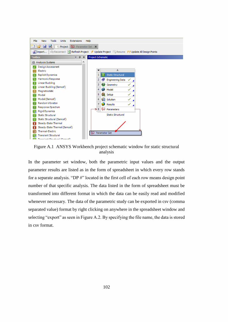
102

Figure A.1 ANSYS Workbench project schematic window for static structural

analysis

In the parameter set window, both the parametric input values and the output

parameter results are listed as in the form of spreadsheet in which every row stands

for a separate analysis. “DP #” located in the first cell of each row means design point

number of that specific analysis. The data listed in the form of spreadsheet must be

transformed into different format in which the data can be easily read and modified

whenever necessary. The data of the parametric study can be exported in csv (comma

separated value) format by right clicking on anywhere in the spreadsheet window and

selecting “export” as seen in Figure A.2. By specifying the file name, the data is stored

in csv format.

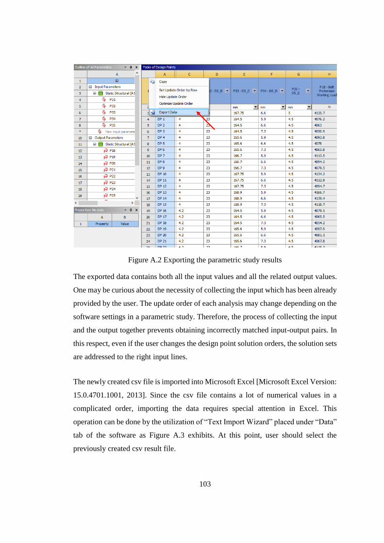
103

Figure A.2 Exporting the parametric study results

The exported data contains both all the input values and all the related output values.

One may be curious about the necessity of collecting the input which has been already

provided by the user. The update order of each analysis may change depending on the

software settings in a parametric study. Therefore, the process of collecting the input

and the output together prevents obtaining incorrectly matched input-output pairs. In

this respect, even if the user changes the design point solution orders, the solution sets

are addressed to the right input lines.

The newly created csv file is imported into Microsoft Excel [Microsoft Excel Version:

15.0.4701.1001, 2013]. Since the csv file contains a lot of numerical values in a

complicated order, importing the data requires special attention in Excel. This

operation can be done by the utilization of “Text Import Wizard” placed under “Data”

tab of the software as Figure A.3 exhibits. At this point, user should select the

previously created csv result file.

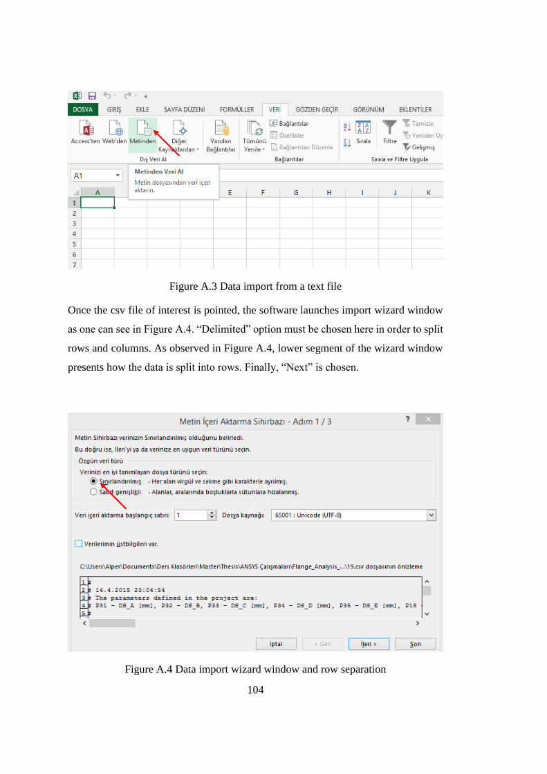
104

Figure A.3 Data import from a text file

Once the csv file of interest is pointed, the software launches import wizard window

as one can see in Figure A.4. “Delimited” option must be chosen here in order to split

rows and columns. As observed in Figure A.4, lower segment of the wizard window

presents how the data is split into rows. Finally, “Next” is chosen.

Figure A.4 Data import wizard window and row separation

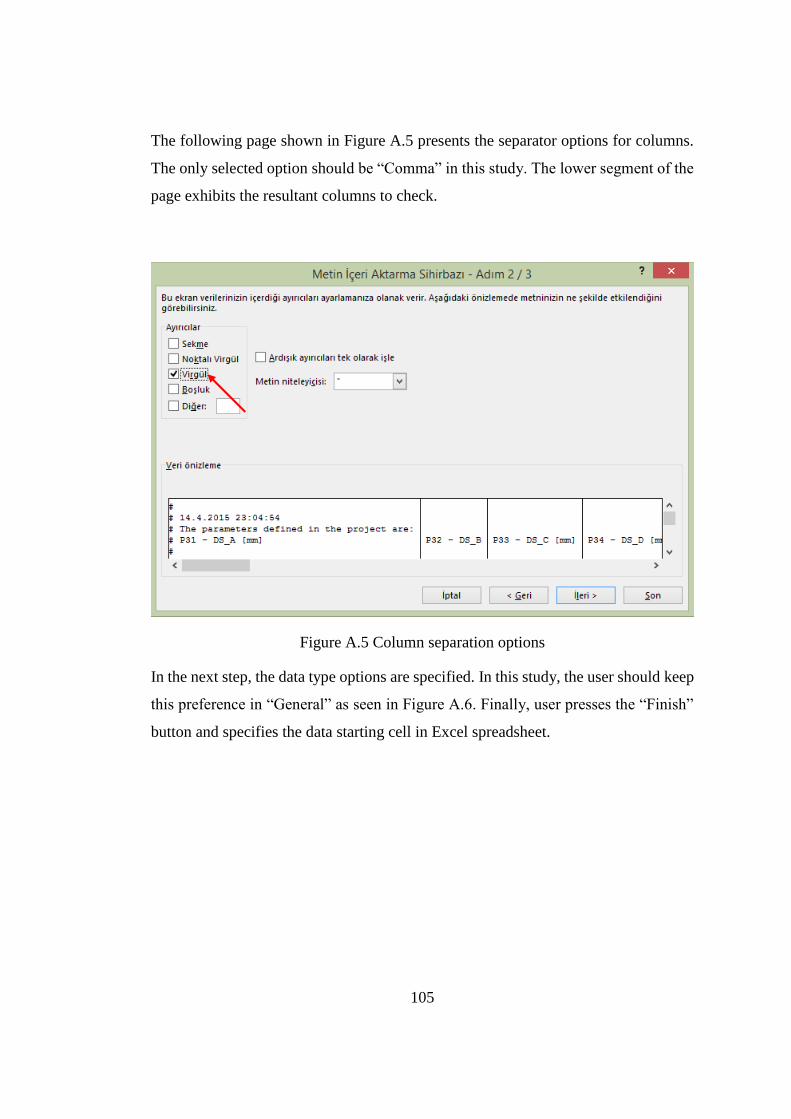
105

The following page shown in Figure A.5 presents the separator options for columns.

The only selected option should be “Comma” in this study. The lower segment of the

page exhibits the resultant columns to check.

Figure A.5 Column separation options

In the next step, the data type options are specified. In this study, the user should keep

this preference in “General” as seen in Figure A.6. Finally, user presses the “Finish”

button and specifies the data starting cell in Excel spreadsheet.

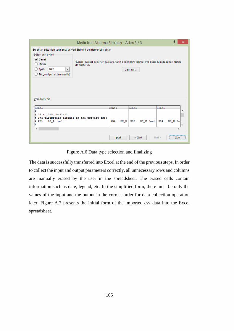
106

Figure A.6 Data type selection and finalizing

The data is successfully transferred into Excel at the end of the previous steps. In order

to collect the input and output parameters correctly, all unnecessary rows and columns

are manually erased by the user in the spreadsheet. The erased cells contain

information such as date, legend, etc. In the simplified form, there must be only the

values of the input and the output in the correct order for data collection operation

later. Figure A.7 presents the initial form of the imported csv data into the Excel

spreadsheet.

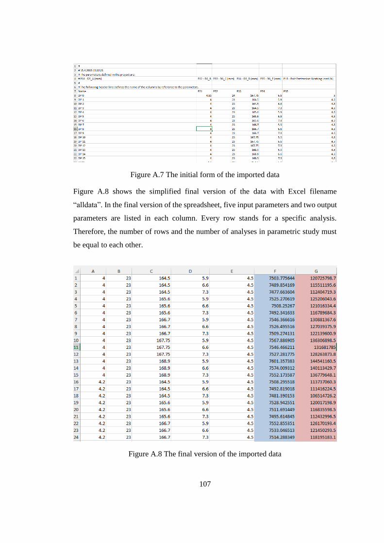
107

Figure A.7 The initial form of the imported data

Figure A.8 shows the simplified final version of the data with Excel filename

“alldata”. In the final version of the spreadsheet, five input parameters and two output

parameters are listed in each column. Every row stands for a specific analysis.

Therefore, the number of rows and the number of analyses in parametric study must

be equal to each other.

Figure A.8 The final version of the imported data

108

The example conducted in this study comprises five geometric input parameters, two

loading (the bolt pretension and the axial external force) input parameters, and two

output parameters (the bolt force reaction in N and the flange stress in MPa). Table

A.1 lists input parameters with the upper and lower limit values. The parametric

analysis database is created with these limits and the ANN is trained with these limits

as well. Table A.2 presents the parametric input values for each variable. All of the

parametric input values of the variables are crossed with each other to obtain the FEA

database covering all combinations. In this respect, a set of 540 (4x3x5x3x3=540)

design points exists when all geometric input values are crossed. In the same way,

the number of the loading input combinations is equal to 25 (5x5=25). As a result,

there are 13500 (540x25=13500) design points in the FEA database in total.

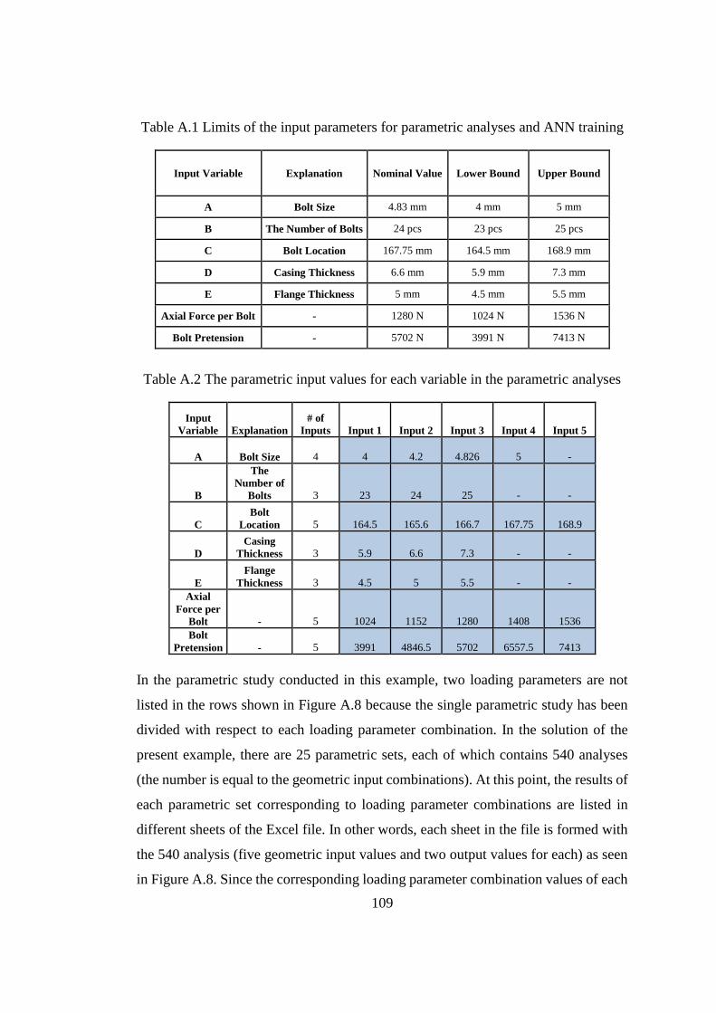
109

Table A.1 Limits of the input parameters for parametric analyses and ANN training

Input Variable Explanation Nominal Value Lower Bound Upper Bound

A Bolt Size 4.83 mm 4 mm 5 mm

B The Number of Bolts 24 pcs 23 pcs 25 pcs

C Bolt Location 167.75 mm 164.5 mm 168.9 mm

D Casing Thickness 6.6 mm 5.9 mm 7.3 mm

E Flange Thickness 5 mm 4.5 mm 5.5 mm

Axial Force per Bolt - 1280 N 1024 N 1536 N

Bolt Pretension - 5702 N 3991 N 7413 N

Table A.2 The parametric input values for each variable in the parametric analyses

Input

Variable Explanation

# of

Inputs Input 1 Input 2 Input 3 Input 4 Input 5

A Bolt Size 4 4 4.2 4.826 5 -

B

The

Number of

Bolts 3 23 24 25 - -

C

Bolt

Location 5 164.5 165.6 166.7 167.75 168.9

D

Casing

Thickness 3 5.9 6.6 7.3 - -

E

Flange

Thickness 3 4.5 5 5.5 - -

Axial

Force per

Bolt - 5 1024 1152 1280 1408 1536

Bolt

Pretension - 5 3991 4846.5 5702 6557.5 7413

In the parametric study conducted in this example, two loading parameters are not

listed in the rows shown in Figure A.8 because the single parametric study has been

divided with respect to each loading parameter combination. In the solution of the

present example, there are 25 parametric sets, each of which contains 540 analyses

(the number is equal to the geometric input combinations). At this point, the results of

each parametric set corresponding to loading parameter combinations are listed in

different sheets of the Excel file. In other words, each sheet in the file is formed with

the 540 analysis (five geometric input values and two output values for each) as seen

in Figure A.8. Since the corresponding loading parameter combination values of each

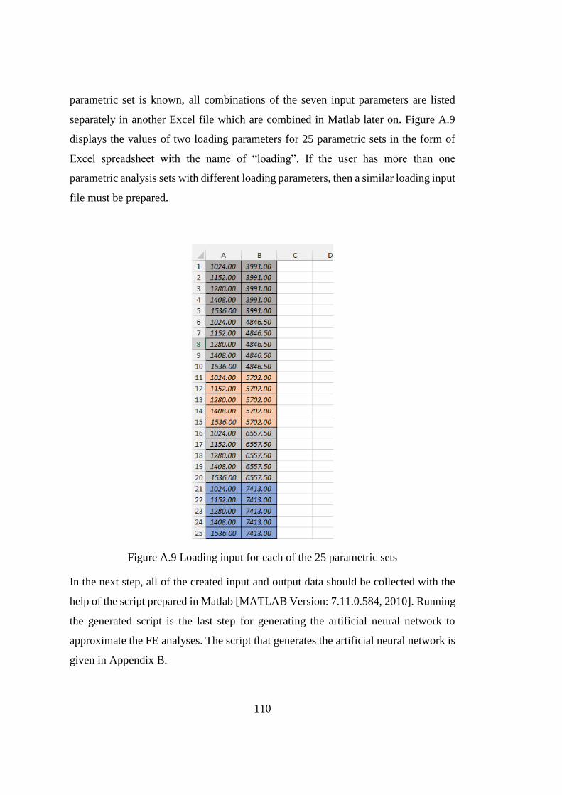
110

parametric set is known, all combinations of the seven input parameters are listed

separately in another Excel file which are combined in Matlab later on. Figure A.9

displays the values of two loading parameters for 25 parametric sets in the form of

Excel spreadsheet with the name of “loading”. If the user has more than one

parametric analysis sets with different loading parameters, then a similar loading input

file must be prepared.

Figure A.9 Loading input for each of the 25 parametric sets

In the next step, all of the created input and output data should be collected with the

help of the script prepared in Matlab [MATLAB Version: 7.11.0.584, 2010]. Running

the generated script is the last step for generating the artificial neural network to

approximate the FE analyses. The script that generates the artificial neural network is

given in Appendix B.

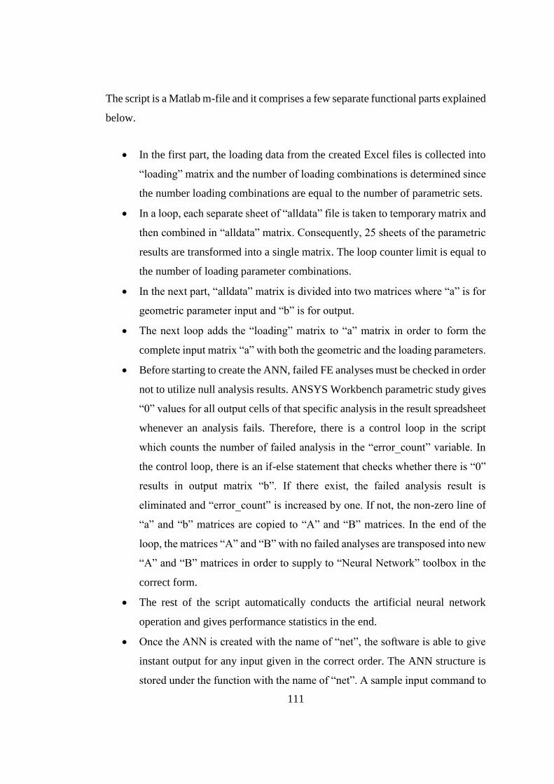
111

The script is a Matlab m-file and it comprises a few separate functional parts explained

below.

In the first part, the loading data from the created Excel files is collected into

“loading” matrix and the number of loading combinations is determined since

the number loading combinations are equal to the number of parametric sets.

In a loop, each separate sheet of “alldata” file is taken to temporary matrix and

then combined in “alldata” matrix. Consequently, 25 sheets of the parametric

results are transformed into a single matrix. The loop counter limit is equal to

the number of loading parameter combinations.

In the next part, “alldata” matrix is divided into two matrices where “a” is for

geometric parameter input and “b” is for output.

The next loop adds the “loading” matrix to “a” matrix in order to form the

complete input matrix “a” with both the geometric and the loading parameters.

Before starting to create the ANN, failed FE analyses must be checked in order

not to utilize null analysis results. ANSYS Workbench parametric study gives

“0” values for all output cells of that specific analysis in the result spreadsheet

whenever an analysis fails. Therefore, there is a control loop in the script

which counts the number of failed analysis in the “error_count” variable. In

the control loop, there is an if-else statement that checks whether there is “0”

results in output matrix “b”. If there exist, the failed analysis result is

eliminated and “error_count” is increased by one. If not, the non-zero line of

“a” and “b” matrices are copied to “A” and “B” matrices. In the end of the

loop, the matrices “A” and “B” with no failed analyses are transposed into new

“A” and “B” matrices in order to supply to “Neural Network” toolbox in the

correct form.

The rest of the script automatically conducts the artificial neural network

operation and gives performance statistics in the end.

Once the ANN is created with the name of “net”, the software is able to give

instant output for any input given in the correct order. The ANN structure is

stored under the function with the name of “net”. A sample input command to

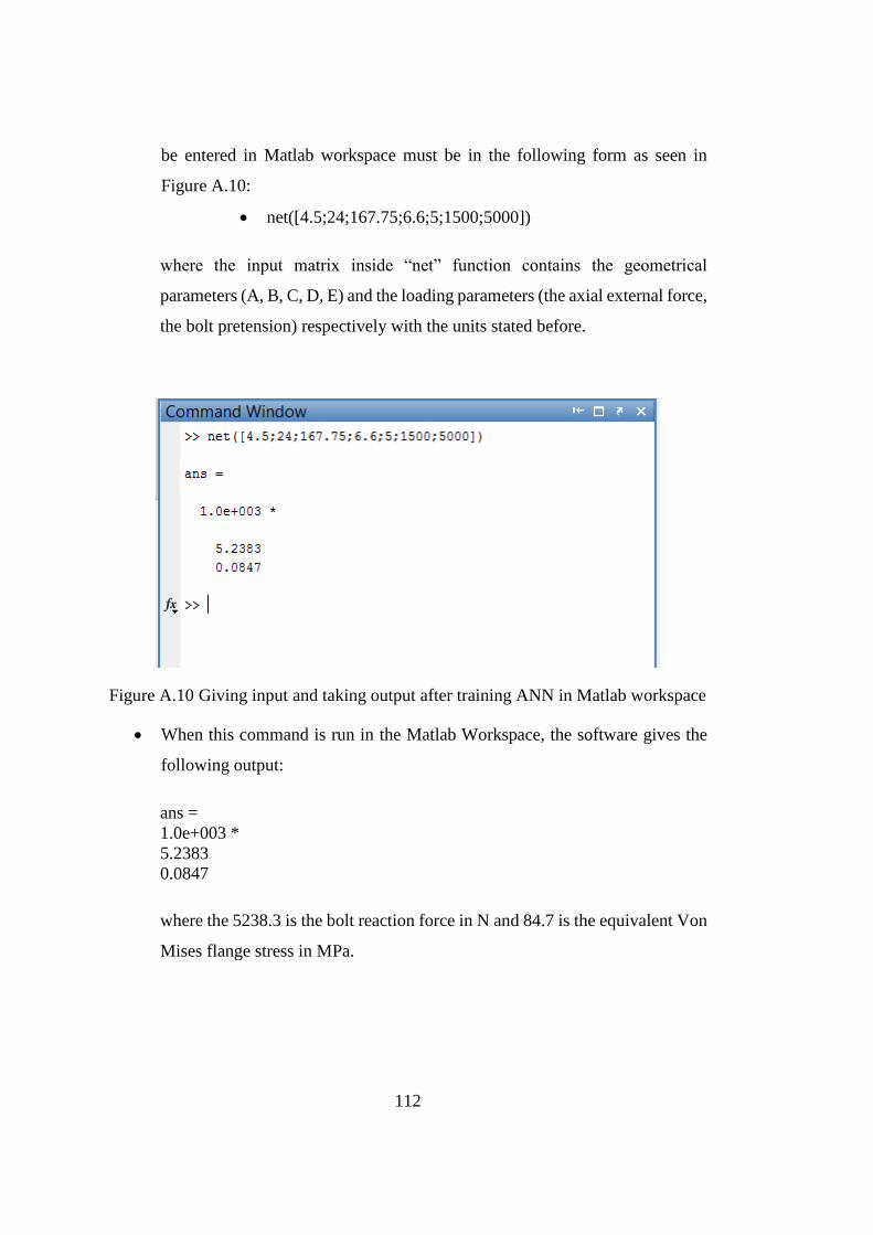
112

be entered in Matlab workspace must be in the following form as seen in

Figure A.10:

net([4.5;24;167.75;6.6;5;1500;5000])

where the input matrix inside “net” function contains the geometrical

parameters (A, B, C, D, E) and the loading parameters (the axial external force,

the bolt pretension) respectively with the units stated before.

Figure A.10 Giving input and taking output after training ANN in Matlab workspace

When this command is run in the Matlab Workspace, the software gives the

following output:

ans =

1.0e+003 *

5.2383

0.0847

where the 5238.3 is the bolt reaction force in N and 84.7 is the equivalent Von

Mises flange stress in MPa.

113

APPENDIX B

THE ARTIFICIAL NEURAL NETWORK SETUP SCRIPT

%Alper YILDIRIM

%Artificial Neural Network Code to Approximate Bolted Flange Connection %Analyses

clear all clc

%Collecting inputs

loading=xlsread('loading.xlsx'); %Axial force and bolt pretension input

%parameters of each parameteric set is collected here.

num_load=size(loading,1); %Total number of loading variables combination

%(equals to analysis sets)

alldata=[]; %"alldata" matrix is defined as an empty matrix.

%Taking ANSYS resultant datasheets into system

for i=1:1:num_load; %the number of loadin input combinations which is equal

%to the number of parametric data sets.

num_sheet=sprintf('Sayfa%d',i)

%Each sheet of "alldata.xlsx" contains the five geometric input

%parameters and two output parameters of a parameteric set. Since there are

%25 parametric sets, 25 sheets exist in this file as well temp=xlsread('alldata.xlsx',num_sheet);

alldata=[alldata;temp]; %Uniting results of all analysis datasheets

%in single matrix in Matlab

end

%Defining the numbers of parameters

num_geo=size(temp,1); %Total number of geometric variables combination

num_analy=num_load*num_geo; %Total number of all variables combination num_par=7; %Total number of input parameters

%Defining the initial input and output matrices of ANN %"a" matrix is ANN training input matrix and "b" is corresponding ANN %target matrix. In this step The first five columns consisting of geometric

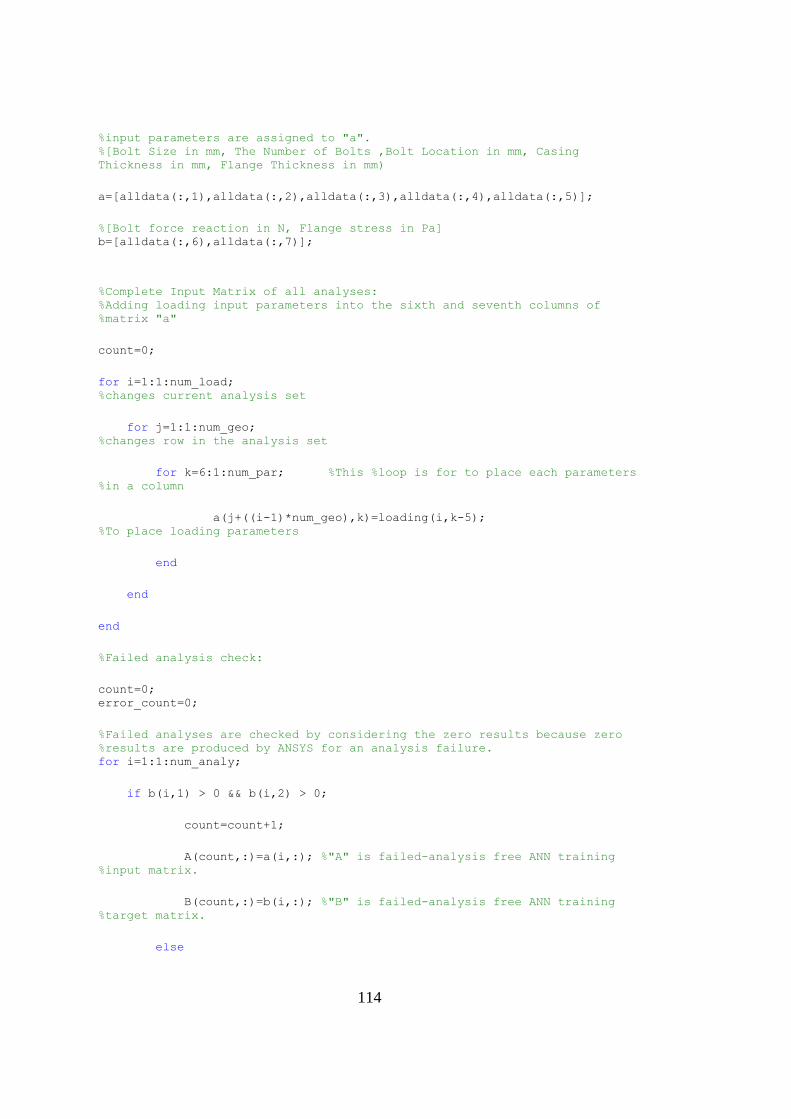
114

%input parameters are assigned to "a". %[Bolt Size in mm, The Number of Bolts ,Bolt Location in mm, Casing

Thickness in mm, Flange Thickness in mm)

a=[alldata(:,1),alldata(:,2),alldata(:,3),alldata(:,4),alldata(:,5)];

%[Bolt force reaction in N, Flange stress in Pa] b=[alldata(:,6),alldata(:,7)];

%Complete Input Matrix of all analyses: %Adding loading input parameters into the sixth and seventh columns of

%matrix "a"

count=0;

for i=1:1:num_load;

%changes current analysis set

for j=1:1:num_geo;

%changes row in the analysis set

for k=6:1:num_par; %This %loop is for to place each parameters

%in a column

a(j+((i-1)*num_geo),k)=loading(i,k-5);

%To place loading parameters

end

end

end

%Failed analysis check:

count=0; error_count=0;

%Failed analyses are checked by considering the zero results because zero %results are produced by ANSYS for an analysis failure. for i=1:1:num_analy;

if b(i,1) > 0 && b(i,2) > 0;

count=count+1;

A(count,:)=a(i,:); %"A" is failed-analysis free ANN training

%input matrix.

B(count,:)=b(i,:); %"B" is failed-analysis free ANN training

%target matrix.

else

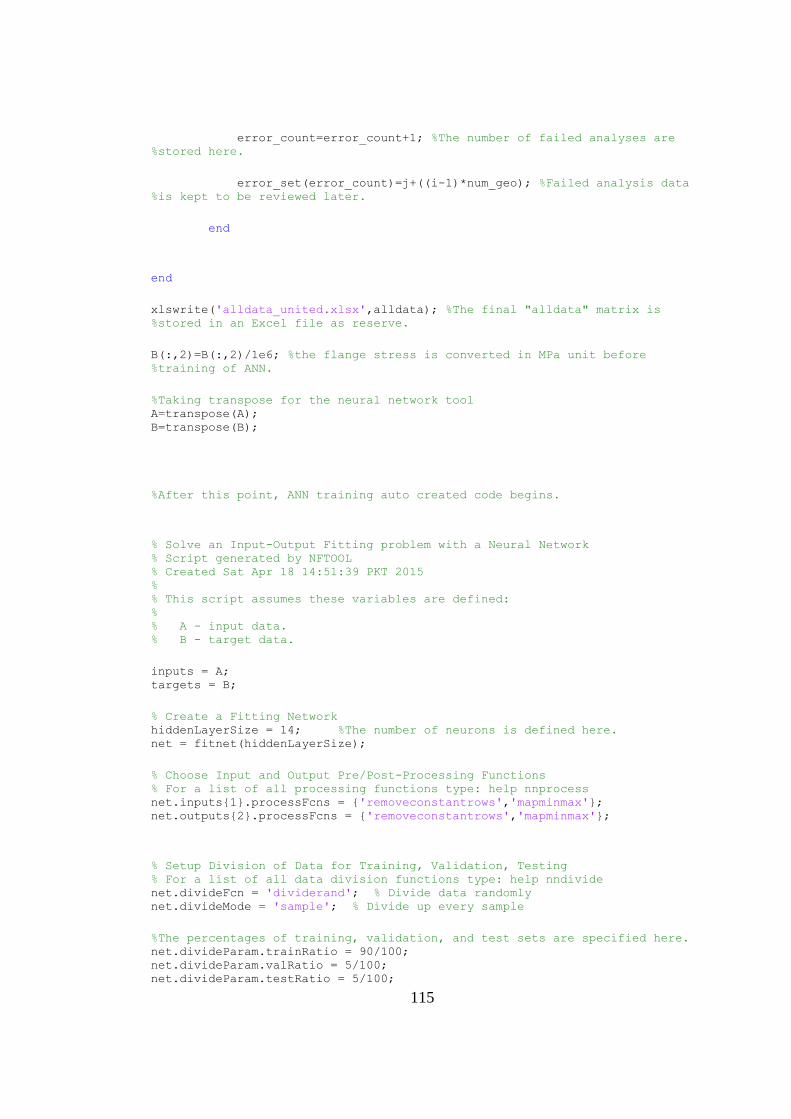
115

error_count=error_count+1; %The number of failed analyses are

%stored here.

error_set(error_count)=j+((i-1)*num_geo); %Failed analysis data

%is kept to be reviewed later.

end

end

xlswrite('alldata_united.xlsx',alldata); %The final "alldata" matrix is

%stored in an Excel file as reserve.

B(:,2)=B(:,2)/1e6; %the flange stress is converted in MPa unit before

%training of ANN.

%Taking transpose for the neural network tool A=transpose(A); B=transpose(B);

%After this point, ANN training auto created code begins.

% Solve an Input-Output Fitting problem with a Neural Network % Script generated by NFTOOL % Created Sat Apr 18 14:51:39 PKT 2015 % % This script assumes these variables are defined: % % A - input data. % B - target data.

inputs = A; targets = B;

% Create a Fitting Network hiddenLayerSize = 14; %The number of neurons is defined here. net = fitnet(hiddenLayerSize);

% Choose Input and Output Pre/Post-Processing Functions % For a list of all processing functions type: help nnprocess net.inputs{1}.processFcns = {'removeconstantrows','mapminmax'}; net.outputs{2}.processFcns = {'removeconstantrows','mapminmax'};

% Setup Division of Data for Training, Validation, Testing % For a list of all data division functions type: help nndivide net.divideFcn = 'dividerand'; % Divide data randomly net.divideMode = 'sample'; % Divide up every sample

%The percentages of training, validation, and test sets are specified here. net.divideParam.trainRatio = 90/100; net.divideParam.valRatio = 5/100; net.divideParam.testRatio = 5/100;

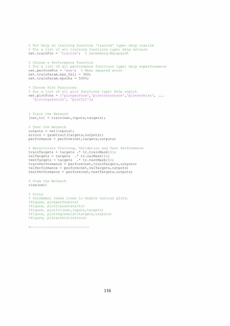
116

% For help on training function 'trainlm' type: help trainlm % For a list of all training functions type: help nntrain net.trainFcn = 'trainlm'; % Levenberg-Marquardt

% Choose a Performance Function % For a list of all performance functions type: help nnperformance net.performFcn = 'mse'; % Mean squared error net.trainParam.max_fail = 300; net.trainParam.epochs = 5000;

% Choose Plot Functions % For a list of all plot functions type: help nnplot net.plotFcns = {'plotperform','plottrainstate','ploterrhist', ... 'plotregression', 'plotfit'};

% Train the Network [net,tr] = train(net,inputs,targets);

% Test the Network outputs = net(inputs); errors = gsubtract(targets,outputs); performance = perform(net,targets,outputs)

% Recalculate Training, Validation and Test Performance trainTargets = targets .* tr.trainMask{1}; valTargets = targets .* tr.valMask{1}; testTargets = targets .* tr.testMask{1}; trainPerformance = perform(net,trainTargets,outputs) valPerformance = perform(net,valTargets,outputs) testPerformance = perform(net,testTargets,outputs)

% View the Network view(net)

% Plots % Uncomment these lines to enable various plots. %figure, plotperform(tr) %figure, plottrainstate(tr) %figure, plotfit(net,inputs,targets) %figure, plotregression(targets,outputs) %figure, ploterrhist(errors)

%----------------------------

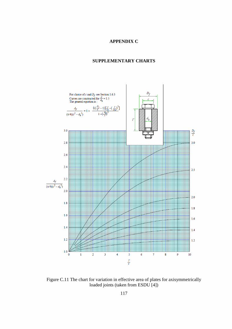
117

APPENDIX C

SUPPLEMENTARY CHARTS

Figure C.11 The chart for variation in effective area of plates for axisymmetrically

loaded joints (taken from ESDU [4])

DEVELOPMENT OF BOLTED FLANGE DESIGN TOOL BASED ON...

Documents

Transcript of DEVELOPMENT OF BOLTED FLANGE DESIGN TOOL BASED ON...