Development of an Educational Environment by Using ...

Lat. Am. J. Phys. Educ. Vol. 15, No. 1, March, 2021 1311-1 http://www.lajpe.org

ISSN 1870-9095

Development of an Educational Environment by Using Graphical User Interfaces Applied to Heat Transfer Problems

Fran Sérgio Lobato1, Fábio de Oliveira Arouca2, Gustavo Barbosa Libotte3,4 1,2School of Chemical Engineering, Federal University of Uberlândia, Brazil. 3National Laboratory for Scientific Computing, Petrópolis, Brazil. 4Polytechnique Institute, Rio de Janeiro State University, Nova Friburgo, Brazil.

E-mail: [email protected]

(Recibido el 12 de diciembre de 2020, aceptado el 15 de febrero de 2021)

Abstract In the last few decades, the development of computational tools has made the approach of more complex case studies in

chemical engineering classrooms more accessible, such as the simulation of nonlinear problems, assessment of the

sensitivity of input parameters in certain models and analysis of physical behavior considering different operating

conditions in a system. In this context, the use of graphical user interfaces represents a typical example of this type of

computational tool that makes classes more dynamic and allows for greater understanding by students, even in more

complex problems. In this work, it is proposed to use graphical user interfaces, developed in Scilab, to improve

learning and engagement in the analysis of heat transfer problems in chemical engineering classrooms. For this

purpose, two classical case studies are simulated and analyzed using the proposed tools. The first considers the heat

transfer in solids and the second considers the Gurney-Lurie charts. The results obtained demonstrate that the use of

graphical user interfaces allows some difficulties to be avoided, such as the understanding and implementation of

numerical methods necessary to solve some problems, besides facilitating the understanding of different physical

aspects, since it provides a visually simplified environment for carrying out different simulations with varied parameter

values and easy access to graphical results.

Keywords: Educational Environment, Graphical User Interface, Scilab, Heat Transfer.

Resumo Nas últimas décadas, o desenvolvimento de ferramentas computacionais têm permitido a abordagem de estudos de caso

mais complexos em salas de aula nos cursos de graduação em engenharia química, como por exemplo a simulação de

problemas não lineares, a avaliação da sensibilidade dos parâmetros de entrada em determinados modelos e a análise do

comportamento físico considerando diferentes condições de operação no sistema em análise. Nesse contexto, o uso de

interfaces gráficas representa um exemplo típico desse tipo de ferramenta computacional que torna as aulas mais

dinâmicas, permitindo uma maior compreensão dos alunos, mesmo em problemas mais complexos. Neste trabalho,

propõe-se a utilização de interfaces gráficas, desenvolvidas em Scilab, para aprimorar o aprendizado e o engajamento

na análise de problemas de transferência de calor em salas de aula do curso de graduação em engenharia química. Para

essa finalidade, dois estudos de caso clássicos são simulados e analisados a partir das ferramentas propostas. O primeiro

avalia a transferência de calor em sólidos e o segundo considera a análise dos diagramas de Gurney-Lurie. Os

resultados obtidos demonstram que o uso de interfaces gráficas permite que algumas dificuldades sejam minimizadas,

tais como a compreensão e implementação de métodos numéricos necessários à resolução de alguns problemas, além

de facilitar o entendimento de diversos aspectos físicos, uma vez que a metodologia proposta apresenta um ambiente

visualmente simplificado onde podem ser realizadas inúmeras simulações e de fácil acesso aos resultados gráficos.

Palavras-chave: Ambiente Educacional, Interface Gráfica, Scilab, Transferência de Calor.

I. INTRODUCTION

The study of transport phenomena encompasses several

areas in chemical engineering with many applications in

different fields of science. In the context of heat transfer

phenomenon, a profusion of applications can be found in

the literature, such as heat transfer in reactors, distillation

columns, dryers, among others [1, 2, 3]. The mathematical

formulation of problems of this type depends on certain

hypotheses and requires, in general, the application of

numerical methods due to the different levels of complexity

(system of algebraic equations, system of differential

equations, differential-integral system and algebraic-

differential system). As demonstrated by Cartaxo and co-

workers [4] and Golman [5], computer simulations can be

employed to understand chemical models and to produce

knowledge in the teaching of chemical engineering. In this

case, considering certain chemical engineering simulations,

the cost related to laboratory analysis can be reduced. In

addition, the number of experiments needed to understand a

particular process can be optimized [6].

In the academic context, analyzing such problems,

which make use of various mathematical tools, in different

disciplines of undergraduate courses may be not a trivial

Fran S. Lobato, Fábio de O. Arouca and Gustavo B. Libotte


task. This is due to the structure provided by some

universities and the difficulty inherent in working with

analytical and numerical methods. For this reason, in many

of these courses, a large number of student failures can be

observed. Thus, the development of methodological tools

that help the student to understand the different concepts

involved in these disciplines without the need to implement

computational codes represents an area of study with great

importance and applicability.

In the specialized literature, a wide variety of software

to simulate different phenomena can be found. In chemical

engineering, one of the main representatives is the EMSO

simulator (Environment for Modeling, Simulation and

Optimization) [7]. EMSO is a graphical environment that

allows the mathematical modeling of complex systems

under steady state or transient conditions, based on the

selection and coupling of different models. The software

also allows the development of new models using the

simulator's modeling language or using models from the

EMSO Model Library (EML). Despite the great

applicability of EMSO, the need to manipulate source code

and dependence on programming logic is still an obstacle to

its employment in many disciplines. In view of these

possible limitations, we can also mention ANSYS,

FLUENT, COMSOL and MATLAB, which also has great

processing capacity but, in general, depends on

programming skills, despite the fact that these softwares

still require a license for use in certain applications, which

does not guarantee access to the source code. In this case,

possible changes in case studies previously incorporated

into these softwares, in general, cannot be made.

Alternatively, Scilab was developed by the French Institute

for Research in Computer Science and Automation

(INRIA). It is a high-level programming language and a

cross-platform computing environment that provides

powerful tools for scientific applications.

In the educational context, these softwares are used to

solve problems with different levels of complexity in a

classroom environment. Edgar and co-workers [8] assessed

the simulation in control education of classical process in

chemical engineering (distillation columns, chemical

reactors, pH processes, microelectronics, and biological

processes). Bordeianu and co-workers [9] developed a

Scilab code for the study of turbulent flows and maps

considering chaotic systems defined by ordinary differential

equations. Domingues and co-workers [10] described the

design and implementation of two virtual labs (by using

internet) for biochemical engineering education. The first

virtual lab consists of the determination of correlation

between oxygen transfer rate, aeration rate and agitation

power in a reactor. The second virtual lab consists of the

determination of residence time distribution in continuous

tanks series. According to these authors, the advantages in

this kind of implementation are: reduced costs, reduced

experience time, and improved data with no loss of

education efficiency. Komulainen and co-workers [11]

developed a dynamic simulation software based on D-Spice

and K-Spice to solve three different chemical engineering

problems. For this purpose, the following topics were

assessed: basic chemical engineering; operability and safety

analysis; and process control. The experiences of both

teachers and students were analyzed. According to these

authors, the experiences confirm that dynamic simulators

provide realistic training and can be successfully integrated

into undergraduate and graduate teaching, laboratory

courses and research. Rahman and co-workers [12]

developed a MATLAB code involving chemical and

biochemical engineering education. Llanos and co-workers

[13] describes a laboratory routine designed to help

chemical engineering students understand the basic

concepts of corrosion. For this purpose, the corrosion rates

of six different materials have been calculated to assess the

effects of the corrosion environment and to apply corrosion

prevention methods.

To make the interaction between user and source code

more accessible, graphical user interfaces (GUIs) have been

increasingly used in the classroom. Thus, tasks such as

implementation and choosing a methodology to solve

certain problems can be avoided. Taking into account

simple commands, the user can define parameters, model

and simulation characteristics, and perform sensitivity

analysis. In addition, a visual illustration of how results

change due to various variables reinforces the lessons [14].

In literature, various works considering the use of GUIs

and other similar approaches can be found. Wilson and

Marcotte [15] developed a graphical interface by using

LabVIEW 4.0 to analyze the gas-phase reaction kinetics of

cyclopentene vapor pyrolysis. This code was used to

produce a graphical interface with the same look and feel as

a physical data station with all its switches, digital readouts,

and strip chart recorders. Tsai [16] developed a post-

processor by using GUI tools in Scilab to visualize fuel rod

burnup analysis data. This code associates a GUI

(numerical results with 2-D and 3-D graphs) with

animations regarding the fuel temperature distribution.

Depcik and Assanis [14] developed several GUIs in an

educational engineering environment, considering different

software options and programming languages (FORTRAN,

C, JAVA, MATLAB and VISUAL BASIC) to solve a

cavity flow problem. In this problem, the flow inside the

box is driven by a plate moving at a constant velocity. The

governing equations of motion for the flow within the box

are the incompressible two-dimensional Navier-Stokes

equations.

Kaddouri and co-workers [17] proposed a novel

software called NLSoft, developed for the design of

nonlinear controllers based on the well-known feedback

linearization technique. This software package contains

several symbolic manipulation modules, which includes

differential geometric tools for the design and simulation of

control systems. In addition, the NLSoft package presents a

user-friendly GUI that incorporates the calculation time of

linearizing control laws considering several digital signal

processors characteristics. Andreatos and Zagorianos [18]

developed a GUI tool for teaching and learning automatic

control systems by using MATLAB. The proposed tool was

applied to the control of a rigid supersonic aircraft with

linear dynamics described by a simple single-input single-



output transfer function that depends on the airplane

structure and flight parameters. Magyar and Zakova [19]

proposed a Scilab-based Remote Control applied to two

experiments: the thermo-optical and the hydraulic plant.

The implemented code is based on open technologies

whereby the kernel of the application is built using XCOS

(control-oriented toolbox).

Vieira and co-workers [20] also applied the XCOS

package in Scilab to study two case studies---stirred tank

with heating and continuous stirred tank reactor with van de

Vusse kinetic. For this purpose, they focused on the

development of control loops block diagrams, PID control

tuning, and process response analysis. He and Li [21]

proposed a MATLAB-based GUI to evaluate the

Hydrogeochemical Diagram. In this project, the different

diagrams can be obtained by user (Piper diagram, Gibbs

diagram, Wilcox diagram and PI classification diagram). As

mentioned by the authors, all the codes of the graphical

interface can be freely accessed and adjusted by users

according to their needs. Molina and co-workers [22]

developed the KBR (Kinetics in Batch Reactors) code. This

is a MATLAB-based application with a friendly GUI for

chemical kinetic model simulation and parameter

estimation.

The School of Chemical Engineering at the Federal

University of Uberlândia (Brazil) has been promoting a

pilot project that concerns the development of GUIs, using

Scilab, for classroom assistance in the discipline of Heat

Transfer. Each GUI developed addresses a specific case

study in chemical engineering and aims to complement the

work of students in the classroom, as well as to promote

new educational activities in e-Learning, that is, these

platforms allow better preparation of students in relation to

physical concepts learned during classes.

In this work, our objective is to present the structure of

two graphical environments for the treatment of heat

transfer problems. For this purpose, we use Scilab to

analyze two classical case studies. The first one concerns

the simulation of heat transfer in solids and the second one

considers the determination of Gurney-Lurie Charts. This

work is structured as follows. Section II presents the

general characteristics about Scilab and its use for creating

GUIs. Section III presents a mathematical description for

the two case studies analyzed. Section IV describes the

schematic representation of the GUIs proposed. The

applications regarding the above mentioned case studies are

presented in Section V. Finally, the conclusions are

presented in the last section.

II. SCILAB AND THE CREATION OF GUIS

Scilab is a free and open source platform, based on the

well-known MATLAB, which provides powerful tools for

numerical computing and a high-level numerically oriented

programming language. The software allows the definition

of different types of operations, with an extensive range of

built-in mathematical functions. In addition, it presents the

possibility of interaction with other programming

languages, 2-D and 3-D graphics library, functions for

integration of ordinary differential equations and algebraic-

differential equations, tools for handling classic and robust

control, packages for optimization, signal and image

processing, parallel architecture, among other features.

Recently, a toolbox designed to provide the interactive

creation of GUIs, called GuiBuilder, has been incorporated

into Scilab. The toolbox can be easily installed (through a

single command) using ATOMS (AuTomatic mOdules

Management for Scilab), which is the Scilab's repository for

packaged extension modules. The GUI development

environment provided by the GuiBuilder package can be

seen in Fig. 1.

FIGURE 1. GUI Builder environment composed of the palette of

widgets.

In the window shown in Fig. 2, all the essential widgets

(graphic objects) for creating a graphical interface are

available, as well as some options for handling the

properties of such objects. The creation is simple and

intuitive, and can be mostly driven by drag-and-drop tasks.

The combination between these two figures represents the

window in which the graphic objects can be inserted. The

toolbox provides the possibility of immediate visual

inspection, as the graphical interface is created, which

makes easier the achievement of the expected result. After

creating the GUI, the toolbox generates the corresponding

source code, in Scilab language, which can be manipulated

by the user.

In fact, the creation of GUIs itself is not the focus of this

work, but the discussion on its use and importance in the

field of teaching, especially in chemical engineering

courses. Therefore, we are not going to detail its creation

procedure, but focus our discussion on the advantages that

the use of graphical interfaces can bring to the dynamics of

classes and to the understanding of students about analyzes

that can hardly be carried out effectively without the use of

computational resources. The case studies discussed in this

work are presented below, which are further included in the

proposed GUIs.



FIGURE 2. GUI Builder environment composed of the graphical

window.

III. CASE STUDIES: HEAT TRANSFER IN A

SOLID BODY AND GURNEY-LURIE CHARTS

In this section, the mathematical descriptions of two case

studies are presented. The first case study considers the

simulation of heat transfer in a solid body, which is initially

at a temperature T0 and is suddenly exposed to the

environment (air) at a temperature T∞. In this model, the

following simplifications and assumptions are considered

[23]: i) the rate of heat transfer by convection is much

higher than the rate of heat transfer by radiation to other

surfaces or to open spaces; ii) surrounding air has a mass

such that its temperature - at least for positions far from the

body surface - remains constant and equal to T∞; iii) no

chemical reaction or any other form of energy source is

present in the body; iv) within the range of temperatures

involved in the process, no phase change is verified; v)

volume of the body is small and its thermal conductivity is

relatively high, and does not change too much within the

range of temperature of the process.

Mathematically, this heat transfer process can be

represented by:

( ) ,

= − −

p

dT AT T

dt VC (1)

0(0) ,=T T (2)

where t is the time (and t∞ is the final time), T is the

temperature, ρ is the density, Cp is the specific heat, A is the

heat exchange area, V is the volume and α is the heat

transfer coefficient. In order to simulate the results of this

ordinary differential equation on the graphical interface, we

employ the classic fourth-order Runge-Kutta method

(referred to here as RK4). However, note that the analysis

of these numerical results must be an extension of the

analytical solution developed during the classes, which can

be obtained using the method of separation of variables

(more details on this solution can be seen in [23]).

The second case study considers the determination of

Gurney-Lurie charts [24]. These charts can be used to

represent solutions of mathematical models designed to

describe non-steady state heat conduction in prototype

geometries such as a flat plate, infinite length cylinder or

sphere. In general, the use of these charts is restricted to the

following conditions [25]: i) the solid is homogeneous; ii)

the thermal diffusivity is constant; iii) there is no source of

heat generation; iv) the initial temperature is uniform; v) the

system is forced by a change in ambient temperature; vi)

the heat transfer process is one-dimensional and; vii) the

process is transient.

Considering such conditions, the process described by

one-dimensional variables can be modeled by the following

partial differential equation, together with the initial and

boundary conditions [25]:

2

2,

= +

(3)

0, 0, 0,

= =

(4)

Bi , 1, 0,

− = =

(5)

1, 0, 0 1, = = (6)

where θ, φ and τ represents temperature, geometric

coordinates and time, respectively, Bi is the Biot Number,

and Φ is a parameter that defines the type of geometry (Φ =

0 stands for flat plate, Φ = 1 for cylinder and Φ = 2 for

sphere).

To solve this model, the well-known Method of Lines is

used [26]. This approach consists in transforming the

original model (partial differential equation) into a system

of ordinary differential equations by using, for instance, the

finite difference formulas. Thus, by defining the number of

discretization points for φ, using approximations for first

and second order derivatives, and evaluating the boundary

conditions, the original model can be converted into a

system of ordinary differential equations. The resulting

system can be solved using RK4, as employed here.

IV. STRUCTURE AND FEATURES OF THE

PROPOSED GUIS

In this section, a brief description of the GUIs proposed in

this work is presented, mainly in relation to their features.

For the sake of didactic and previous experiences, it is

convenient to organize both case studies in two separate

GUIs, in order to make the use simplified. Naturally, it is

possible to develop a platform that brings together these

and several other problems of the same nature. However,

one surmises that encompassing several functionalities in a

single GUI may represent an increase in its complexity,

which is not desirable from the point of view of usability.



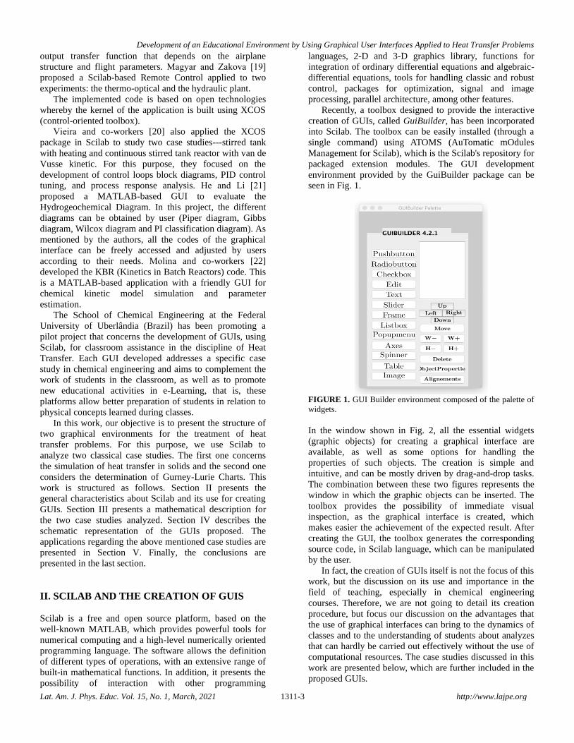
A. Heat Transfer in a Solid

Figure 3 shows the GUI proposed in this work for the heat

transfer problem in a solid. Initially, one may note that the

structure of the application is simple: the upper left frame

(Model) shows fundamental information about the model,

referring to equation (1) and equation (2). Model

parameters (T∞, T0, ρ, Cp, A, V, α and t∞) are listed in the

frame below, followed by the respective units of

measurement, and a field to input the desired value for a

simulation. The same goes for the only adjustable

parameter of the RK4 method, the number of points for

discretization N. In turn, the empty frame, which covers

most of the visible area of the GUI, is intended for the

graphical display of the results. Finally, the Simulate and

Clear buttons are responsible for starting a simulation and

clearing existing results, respectively.

FIGURE 3. Graphical interface for the Heat Transfer in a Solid

problem.

In the menu bar, the option Problem Description shows, in

a new window, an essential description of the simulated

model in the GUI, as can be seen in Fig. 4.

FIGURE 4. Brief description of the heat transfer problem in a

solid.

In order to execute a simulation, the operation of the GUI is

very intuitive: the user must only input all the values of the

parameters listed in the Model Parameters and Fourth-

Order Runge-Kutta frames, and click on the Simulate

button. Then the entered values are used in the simulation

of the heat transfer problem in a solid, showing the

temperature profile as a function of time.

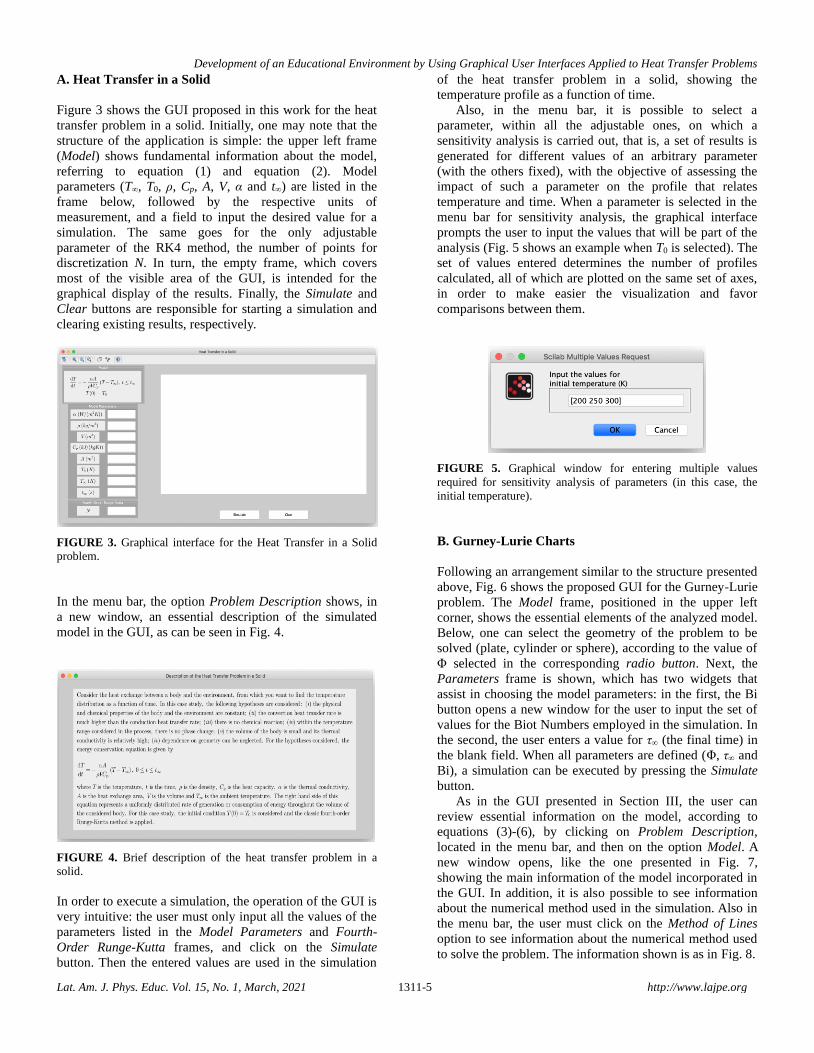
Also, in the menu bar, it is possible to select a

parameter, within all the adjustable ones, on which a

sensitivity analysis is carried out, that is, a set of results is

generated for different values of an arbitrary parameter

(with the others fixed), with the objective of assessing the

impact of such a parameter on the profile that relates

temperature and time. When a parameter is selected in the

menu bar for sensitivity analysis, the graphical interface

prompts the user to input the values that will be part of the

analysis (Fig. 5 shows an example when T0 is selected). The

set of values entered determines the number of profiles

calculated, all of which are plotted on the same set of axes,

in order to make easier the visualization and favor

comparisons between them.

FIGURE 5. Graphical window for entering multiple values

required for sensitivity analysis of parameters (in this case, the

initial temperature).

B. Gurney-Lurie Charts

Following an arrangement similar to the structure presented

above, Fig. 6 shows the proposed GUI for the Gurney-Lurie

problem. The Model frame, positioned in the upper left

corner, shows the essential elements of the analyzed model.

Below, one can select the geometry of the problem to be

solved (plate, cylinder or sphere), according to the value of

Φ selected in the corresponding radio button. Next, the

Parameters frame is shown, which has two widgets that

assist in choosing the model parameters: in the first, the Bi

button opens a new window for the user to input the set of

values for the Biot Numbers employed in the simulation. In

the second, the user enters a value for τ∞ (the final time) in

the blank field. When all parameters are defined (Φ, τ∞ and

Bi), a simulation can be executed by pressing the Simulate

button.

As in the GUI presented in Section III, the user can

review essential information on the model, according to

equations (3)-(6), by clicking on Problem Description,

located in the menu bar, and then on the option Model. A

new window opens, like the one presented in Fig. 7,

showing the main information of the model incorporated in

the GUI. In addition, it is also possible to see information

about the numerical method used in the simulation. Also in

the menu bar, the user must click on the Method of Lines

option to see information about the numerical method used

to solve the problem. The information shown is as in Fig. 8.



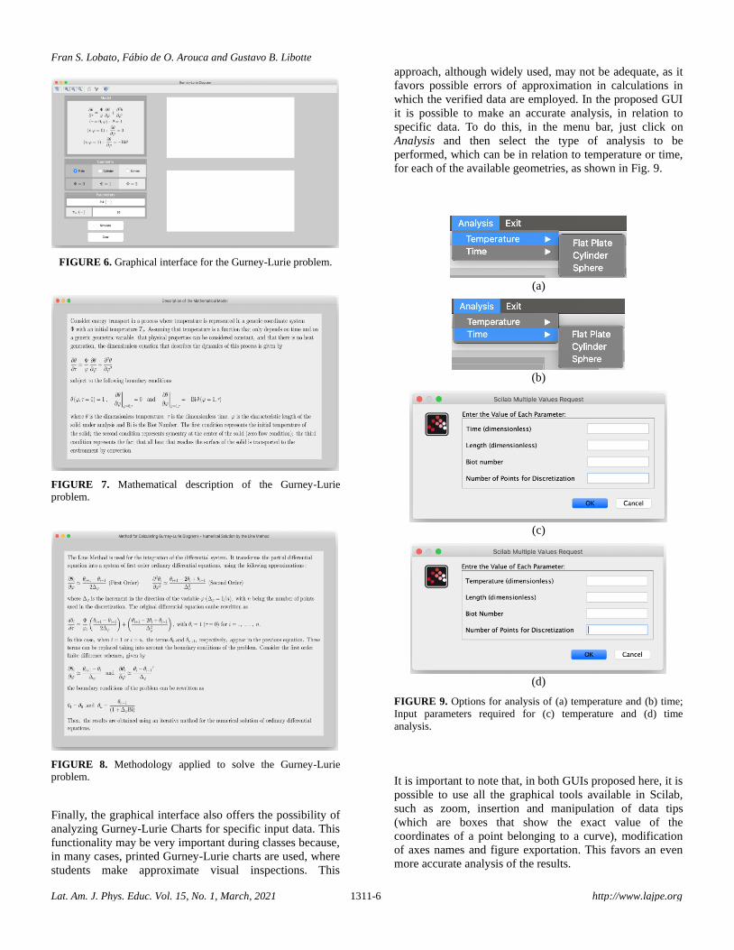
FIGURE 6. Graphical interface for the Gurney-Lurie problem.

FIGURE 7. Mathematical description of the Gurney-Lurie

problem.

FIGURE 8. Methodology applied to solve the Gurney-Lurie

problem.

Finally, the graphical interface also offers the possibility of

analyzing Gurney-Lurie Charts for specific input data. This

functionality may be very important during classes because,

in many cases, printed Gurney-Lurie charts are used, where

students make approximate visual inspections. This

approach, although widely used, may not be adequate, as it

favors possible errors of approximation in calculations in

which the verified data are employed. In the proposed GUI

it is possible to make an accurate analysis, in relation to

specific data. To do this, in the menu bar, just click on

Analysis and then select the type of analysis to be

performed, which can be in relation to temperature or time,

for each of the available geometries, as shown in Fig. 9.

(a)

(b)

(c)

(d)

FIGURE 9. Options for analysis of (a) temperature and (b) time;

Input parameters required for (c) temperature and (d) time

analysis.

It is important to note that, in both GUIs proposed here, it is

possible to use all the graphical tools available in Scilab,

such as zoom, insertion and manipulation of data tips

(which are boxes that show the exact value of the

coordinates of a point belonging to a curve), modification

of axes names and figure exportation. This favors an even

more accurate analysis of the results.



V. RESULTS AND DISCUSSION

This section presents the results and discussions on both

GUIs presented previously.

A. Heat Transfer in a Solid

Figure 10 shows an example simulation of the proposed

GUI for the heat transfer problem in a solid, considering the

parameters α = 100 W/(m2K), ρ = 1000 kg/m3, V = 1 m3, Cp

= 4.2 kJ/(kg K), A = 10 m2, T0 = 290 K, T∞ = 500 K, t∞ = 30

s and N = 100. Under such conditions, the process reaches

the steady state condition, that is, the temperature gradient

over time is equal to zero when T = T∞. If t∞ is much less

than 30 s, this condition cannot be seen on the temperature

distribution curve presented. Taking into account the

dynamics of a classroom, this GUI provides the possibility

to perform successive simulations, with little programmatic

effort, obtaining instant results and providing students

different perspectives on the behavior of the problem and

its results for several input parameters. This favors the

understanding of the mathematical model and reinforces the

behavior of the analytical solution.

FIGURE 10. Typical execution of the heat transfer problem in a

solid, showing the curve that describes the temperature

distribution as a function of time.

Providing a comparative view on the behavior of the curve

that describes temperature as a function of time when

varying a given model parameter can be more convenient

using the Sensitivity Analysis tool. Figure 11 presents the

results of the sensitivity analysis of the model when the

area of the solid varies, keeping the other parameters of the

model fixed. In these results, the temperature profiles are

shown when A = [ 10 20 30 40 50] (m2). Using this tool, it

is clear that the increase in the heat exchange area implies

less time to obtain the steady state, that is, smaller areas

imply smaller volumes of the solid, which is being heated

or cooled. Physically, increasing the heat exchange area

causes a decrease in convective resistance but, on the other

hand, leads to an increase in conductive resistance.

Concepts like these, when shown through examples and

numerical simulations, can be more easily understood by

students.

FIGURE 11. Results for the sensitivity analysis of the area

considered in the model of the heat transfer problem in a solid.

B. Gurney-Lurie Charts

Gurney-Lurie Charts obtained from a typical simulation

considering Bi = [0.1 0.2 0.5 1 2], τ∞ = 10 and Φ = 0 are

presented in Fig 12. Note that the colors of the curves, the

types of markers and the legends are automatically inserted,

which provides a clear reading of the results obtained. For

this application, a fixed number of points for discretization

(N = 100) is programmatically determined, in order to

transform the original partial differential equation into a

system of ordinary differential equations. When clicking on

the Simulate button, the graphical interface also provides

the possibility to perform the simulation with Bi → ∞, as

can be seen in Fig. 12.

FIGURE 12. Typical graphic window for the Gurney-Lurie

problem.

In both sets of results presented in Fig. 12, the temperature

profiles considering the arithmetic and logarithmic scales



for different values of the parameter referring to the Biot

Number are presented. In general, as expected, the

temperature profile is equal to 1 when τ is equal to zero. For

these profiles, the steady state is not reached. In this case,

the parameter τ∞ should be increase.

If we look at transient problems of heat transfer in a

dimensionless form, we have dimensionless temperature

and time, in addition to the Biot Number. If we have a

problem in which Bi is big enough, we also obtain a

dimensionless position, since the spatial gradients do not

disappear. One of the most practical reasons for making our

results dimensionless is their generalization. Since the same

dimensionless equation holds for many different systems,

we can use the same dimensionless response for all of them.

A particularly useful fact of this is that one can tabulate

results from dimensionless solutions to transient problems.

Despite this, tabulated results restrict analyzes to the

existing values and, in addition, do not favor the

verification of the behavior of the results as a whole.

Therefore, it is important to take account of the results more

accurately, given arbitrary input parameters. In this context,

Fig. 13 presents a specific simulation, performed using the

Sensitivity Analysis tool shown in Fig. 9, for the system

temperature in a flat plate, considering the other parameters

defined with the values shown in Fig. 13.

FIGURE 13. Graphical window for estimating the temperature of

the Gurney-Lurie problem for a flat plate.

Indeed, the same analysis can be carried out over time,

taking into account each of the geometries (flat plate,

cylinder or sphere) of the problem.

VI. CONCLUSIONS

In this work, two graphical tools have been proposed,

aiming to solve two heat transfer problems in undergraduate

chemical engineering courses. The main steps of the

proposed methodology are: i) describe the mathematical

modeling of each case study; ii) present the GUIs

considering each case study and a specific numerical

methodology; iii) assess the sensitivity of the parameters

inherent to the model and; iv) insert a description page to

help understand each application.

From the proposed GUIs and the discussion presented,

it is clear that the development of this type of platform

helps teachers in relation to the physical analysis of

chemical problems, especially considering the fact that the

development of computational routines to simulate ordinary

and partial differential equations is avoided. This graphical

tool allows the simulation in a simplified way of

mathematical models which are very common in

undergraduate courses in chemical engineering, as well as

the input of parameters and the generation of graphical

results in a simplified way. As the aspects related to the

implementation and the choice of numerical methodologies

for each application are avoided, access to information

becomes simplified. From the didactic point of view, it is

highlighted that this tool can help teachers in the classroom,

as more complicated case studies can be worked on without

teacher and students having to worry about the

methodologies used to solve these problems.

It is important to mention that, although the problems

considered in this work are relatively simple, the main

objective is the development of an interface that helps the

user in understanding the chemical model, as well as in

physical analysis. Thus, more sophisticated applications can

be developed from this approach. In future works, we aim

to explore other heat transfer models of interest in

undergraduate and graduate courses in chemical

engineering and related areas, such as: i) determining the

critical radius in pipes; ii) the study of extended surface

heat transfer and; iii) Laplace Equation (transient and three-

dimensional), among others.

ACKNOWLEDGEMENTS

The authors are thankful for the financial support provided

to the present research effort by CNPq, FAPEMIG, CAPES

and FAPERJ. Gustavo Libotte is supported by a

postdoctoral fellowship from the Institutional Training

Program (PCI) of the Brazilian National Council for

Scientific and Technological Development (CNPq), grant

number 303185/2020-1, and Carlos Chagas Filho

Foundation for Supporting Research in the State of Rio de

Janeiro, grant number E-26/200.560/2018.

SOFTWARE AVAILABILITY

The source codes of the GUIs proposed in this work can be

requested by contacting Dr. Fran Sérgio Lobato

([email protected]).

REFERENCES

[1] Towler, G. and Sinnott, R., Chemical Engineering

Design, Second Edition (Butterworth-Heinemann, Boston,

2013).

[2] Finlayson, B. A, Introduction to Chemical Engineering

Computing, Second Edition (John Wiley & Sons, Hoboken,

2012).



[3] Duncan T. M. and Reimer, J. A., Chemical Engineering

Design and Analysis: An Introduction, Second Edition

(Cambridge University Press, Cambridge, UK, 2019).

[4] Cartaxo, S. J. M., Silvino, P. F.G. and Fernandes, F. A.

N., Transient Analysis of Shell-and-tube Heat Exchangers

Using an Educational Software, Education for Chemical

Engineers 9, e77-e84 (2014).

[5] Golman, B., Transient Kinetic Analysis of Multipath

Reactions: An Educational Module Using the IPython

Software Package, Education for Chemical Engineers 15,

1-18 (2016).

[6] Skorzinski, E., Shacham, M. and Brauner, N., A

Simulation Program for Modelling Pollutant Dispersion for

Educational Applications, 19th European Symposium on

Computer Aided Process Engineering, Computer Aided

Chemical Engineering Series, Jacek Jezowski and Jan

Thullie (Editors), Elsevier 26, 1233-1238 (2009).

[7] Soares, R. P. and Secchi, A. R. EMSO: A New

Environment for Modelling, Simulation and Optimisation,

European Symposium on Computer Aided Process

Engineering-13, Andrzej Kraslawski and Ilkka Turunen

(Editors), Computer Aided Chemical Engineering Series,

Elsevier 14, 947-952 (2003).

[8] Edgar, T. F., Ogunnaike, B. A. and Muske, K. R., A

Global View of Graduate Process Control Education,

Computers & Chemical Engineering 30, 1763-1774 Papers

form Chemical Process Control VII, (2006).

[9] Bordeianu, C. C., Felea, D., Besliu, C., Jipa, Al.,

Grossu, I. V. A New Version of Scilab Software Package for

the Study of Dynamical Systems, Computer Physics

Communications 180, 2398-2399 (2009).

[10] Domingues, L., Rocha, I., Dourado, F., Alves, M. and

Ferreira, E. C., Virtual Laboratories in (bio)Chemical

Engineering Education, Education for Chemical Engineers,

5, e22-e27 (2010).

[11] Komulainen, T. M., Enemark-Rasmussen, R., Sin, G.,

Fletcher, J. P. and Cameron, D.", Experiences on Dynamic

Simulation Software in Chemical Engineering Education,

Education for Chemical Engineers 7, e153-e162 (2012).

[12] Rahman, N. A., Hussain, M. A., Jahim, J. M.,

Kamaruddin, S. K., Abdullah, S. R. S. and Kamaruddin, M.

Z. F., Integrating Computer Applications Into

Undergraduate Courses: Process Control and Utility

Design, Education for Chemical Engineers 8, e45-e57

(2013).

[13] Llanos, J., Perez, A. and Lucas-Consuegra, A.,

Enhancing the Teaching of Corrosion to Chemical-

Engineering Students through Laboratory Experiments,

Journal of Chemical Education 96, 1029-1032 (2019).

[14] Depcik, C. and Assanis, D. N., Graphical User

Interfaces in an Engineering Educational Environment,

Computer Applications in Engineering Education 13, 48-59

(2005).

[15] Wilson, L. D. and Marcotte, R. E., Graphical Interface

for the Study of Gas-Phase Reaction Kinetics:

Cyclopentene Vapor Pyrolysis, Journal of Chemical

Education 78, 799 (2001).

[16] Tsai, C. W., Visualization of Fuel Rod Burnup

Analysis by Scilab, Nuclear Engineering and Design 265,

341-347 (2013).

[17] Kaddouri, A., Blais, S., Ghribi, M. and Akhrif, O.

NLSOFT: An Interactive Graphical Software for Designing

Nonlinear Controllers, Mathematics and Computers in

Simulation 71, 377-384 (2006).

[18] Andreatos, A. S. and Zagorianos, A. D., Matlab GUI

Application for Teaching Control Systems, World Scientific

and Engineering Academy and Society (WSEAS),

Proceedings of the 6th WSEAS International Conference on

Engineering Education of the 6th WSEAS International

Conference on Engineering Education, 208-211, Rodos

Island, Greece, (2009).

[19] Magyar, Z. and Zakova, K., SciLab Based Remote

Control of Experiments, IFAC Proceedings Volumes, 45,

206-211, 9th IFAC Symposium Advances in Control

Education, (2012).

[20] Vieira, E. B., Busch, W. F., Prata, D. M. and Santos, L.

S., Application of Scilab/Xcos for Process Control Applied

to Chemical Engineering Educational Projects, Computer

Applications in Engineering Education 27, 154-165 (2019).

[21] He, S. and Li P., A MATLAB Based Graphical User

Interface (GUI) for Quickly Producing Widely Used

Hydrogeochemical Diagrams, Geochemistry, 125550,

(2019).

[22] Molina, R., Orcajo, G. and Martinez, F. KBR (Kinetics

in Batch Reactors): a MATLAB-based Application with a

Friendly Graphical User Interface for Chemical Kinetic

Model Simulation and Parameter Estimation, Education for

Chemical Engineers 28, 80-89 (2019).

[23] Souza-Santos, M. L., Analytical and Approximate

Methods in Transport Phenomena, First Edition (CRC

Press, Mechanical Engineering Series, Boca Raton, 2007).

[24] Gurney, H. P. and Lurie, J., Charts for Estimating

Temperature Distributions in Heating or Cooling Solid

Shapes, Industrial & Engineering Chemistry 15, 1170-1172

(1923).

[25] Pandharipande, S. L. and Badhe, Y., Artificial Neural

Networks for Gurney-Lurie and Heisler Charts, Journal of

the Institution of Engineers (India): Chemical Engineering

Division 84, 65-70 (2004).

[26] Schiesser, W. E., The Numerical Method of Lines:

Integration of Partial Differential Equations, First Edition,

(Academic Press, San Diego, 1991).

Development of an Educational Environment by Using ...

Documents

Transcript of Development of an Educational Environment by Using ...