Development of a Preliminary Design Tool for Conventional ... · Development of a Preliminary...
91
Development of a Preliminary Design Tool for Conventional Co-Axial and Tandem Helicopter Configuration Miguel Soares Moniz da Ponte Thesis to obtain the Master of Science Degree in Aerospace Engineering Supervisor: Prof. Filipe Szolnoky Ramos Pinto Cunha Examination Committee Chairperson: Prof. Fernando José Parracho Lau Supervisor: Prof. Filipe Szolnoky Ramos Pinto Cunha Member of the Committee: Prof. André Calado Marta November 2016
Transcript of Development of a Preliminary Design Tool for Conventional ... · Development of a Preliminary...

Development of a Preliminary Design Tool for ConventionalCo-Axial and Tandem Helicopter Configuration
Miguel Soares Moniz da Ponte
Thesis to obtain the Master of Science Degree in
Aerospace Engineering
Supervisor: Prof. Filipe Szolnoky Ramos Pinto Cunha
Examination CommitteeChairperson: Prof. Fernando José Parracho Lau
Supervisor: Prof. Filipe Szolnoky Ramos Pinto CunhaMember of the Committee: Prof. André Calado Marta
November 2016

Resumo
Actualmente, a oferta de uma ferramenta computational gratuita, open source e user friendly, para o designpreliminar de helicopteros e escassa. A ferramenta computacional desenvolvida no ambito desta tese tem oobjectivo de colmatar esta lacuna e ajudar o utililzador no processo de design preliminar de um helicoptero deconfiguracao convencional, co-axial ou tandem. O utilizador tera a possibilidade the selecionar um conjuntovariados de parametros de design (desde o perfil em cada seccao da pa ate a potencia instalada), entre as duasteorias mais desenvolvidas para analise de helicopteros (Teoria do Momento Linear e Teoria dos Elementos dePas) e obter a correspondente curva de potencia necessaria. Analizando os resultados obtidos, o alcance maximo,velocidade de alcance maximo, a autonomia maxima e a velocidade de autonomia maxima, serao calculadas,parametros estes essenciais no design preliminar de uma nova aeronave.A ferramenta foi desenvolvida utilizando a interface grafica do MATLAB e inclui uma base de dados de motores,de perfis e das suas caracterısticas aerodinamicas. Para validacao da ferramenta computacional, tres diferentesmodelos de helicopteros foram selecionados (um para cada configuracao). Utilizando os parametros de designfornecidos pelo fabricante e introduzindo estes valores na ferramenta computacional, correram-se as simulacoes.Os resultados obtidos mostraram-se proximos das caracteristticas reais de performance dos helicopteros sele-cionados. Este facto aumenta a confianca que a ferramenta computacional desenvolvida e capaz de prevercorrectamente as caracterısticas de qualquer novo design.
Palavras-chave: potencia necessaria, parametros de design, teoria do momento linear, teoria dos elementos depas, alcance, autonomia.
i

Abstract
Nowadays, the availability of a free, open source, and user-friendly computational tool for preliminary rotor-craft design is scarce. The computational tool developed in the context of this thesis has the goal to fill thisgap and aid the user in its preliminary design process of an helicopter with conventional, co-axial or tandemconfiguration. The user will have the ability to choose between a wide variety of key design parameters (rangingfrom the airfoil at each blade section to the to the power plant installed), between the 2 most known theoriesdeveloped for rotorcraft (Momentum Theory and Blade Element Theory) and obtain the corresponding powerrequirements curve. Analyzing the results obtained, the maximum range, maximum range speed, enduranceand maximum endurance speed can be computed, which are key aspects for the preliminary design of any newrotorcraft.The tool was developed using the MATLAB graphical user interface and includes a database of engines, airfoilshapes and airfoil characteristics. To evaluate if the tool was predicting accurately the rotorcraft characteristics,three different models of already developed helicopters were selected (one for each configuration). Using thedesign parameters values provided by the manufacturers, and inputting those in the computational tool, thesimulations were launched. The results obtained showed an agreement between the predictions of the tool andthe real performance characteristics of the selected models. This fact increases the confidence that the tooldeveloped is able to predict correctly the characteristics of any new design.
Keywords: power requirements, design parameters, momentum theory, blade element theory, range, endurance.
ii

List of Contents
Resumo i
Abstract ii
Abbreviations and Acronyms viii
Nomenclature ix
1 Introduction 11.1 Goals . . . . . . . . . . . . . . . . . . . . . . . . . . . . . . . . . . . . . . . . . . . . . . . . . . . 11.2 State of the art . . . . . . . . . . . . . . . . . . . . . . . . . . . . . . . . . . . . . . . . . . . . . . 1
2 Theoretical Background 22.1 Momentum Theory Analysis in Hovering flight . . . . . . . . . . . . . . . . . . . . . . . . . . . . 2
2.1.1 Flow Behavior in Hovering Flight . . . . . . . . . . . . . . . . . . . . . . . . . . . . . . . . 22.1.2 Conservation Laws . . . . . . . . . . . . . . . . . . . . . . . . . . . . . . . . . . . . . . . . 32.1.3 Application of Conservation Laws to the Hovering Problem . . . . . . . . . . . . . . . . . 32.1.4 Induced Power . . . . . . . . . . . . . . . . . . . . . . . . . . . . . . . . . . . . . . . . . . 52.1.5 Non-dimensional Coefficients . . . . . . . . . . . . . . . . . . . . . . . . . . . . . . . . . . 52.1.6 Non Ideal Effects on Rotor Performance . . . . . . . . . . . . . . . . . . . . . . . . . . . . 6
2.2 Momentum Theory Analysis in Forward flight . . . . . . . . . . . . . . . . . . . . . . . . . . . . . 72.2.1 Induced Velocity in Forward Flight . . . . . . . . . . . . . . . . . . . . . . . . . . . . . . . 82.2.2 Numerical Solution of Inflow Equation . . . . . . . . . . . . . . . . . . . . . . . . . . . . . 82.2.3 Total Power Equation in Forward Flight . . . . . . . . . . . . . . . . . . . . . . . . . . . . 92.2.4 Extension of Momentum Theory to other Rotor Systems . . . . . . . . . . . . . . . . . . . 9
2.3 Blade Element Analysis in Hovering Flight . . . . . . . . . . . . . . . . . . . . . . . . . . . . . . 132.3.1 Rotor Thrust and Power estimation in Hover . . . . . . . . . . . . . . . . . . . . . . . . . 16
2.4 Blade Element Analysis in Forward Flight . . . . . . . . . . . . . . . . . . . . . . . . . . . . . . . 162.4.1 Rotor Thrust and Power estimation in Forward flight . . . . . . . . . . . . . . . . . . . . 172.4.2 Linear Inflow models . . . . . . . . . . . . . . . . . . . . . . . . . . . . . . . . . . . . . . . 182.4.3 Extension of Blade Element Theory to other Rotor Systems . . . . . . . . . . . . . . . . . 20
2.5 Helicopter Performance . . . . . . . . . . . . . . . . . . . . . . . . . . . . . . . . . . . . . . . . . 212.5.1 Density . . . . . . . . . . . . . . . . . . . . . . . . . . . . . . . . . . . . . . . . . . . . . . 212.5.2 Parasitic Power in Forward Flight . . . . . . . . . . . . . . . . . . . . . . . . . . . . . . . 222.5.3 Tip Losses Estimation . . . . . . . . . . . . . . . . . . . . . . . . . . . . . . . . . . . . . . 232.5.4 Tail Rotor Power . . . . . . . . . . . . . . . . . . . . . . . . . . . . . . . . . . . . . . . . . 242.5.5 Climb Performance . . . . . . . . . . . . . . . . . . . . . . . . . . . . . . . . . . . . . . . . 242.5.6 Maximum Endurance . . . . . . . . . . . . . . . . . . . . . . . . . . . . . . . . . . . . . . 252.5.7 Maximum Range . . . . . . . . . . . . . . . . . . . . . . . . . . . . . . . . . . . . . . . . . 252.5.8 Compressiblity Analysis . . . . . . . . . . . . . . . . . . . . . . . . . . . . . . . . . . . . . 262.5.9 Reverse Flow Analysis . . . . . . . . . . . . . . . . . . . . . . . . . . . . . . . . . . . . . . 272.5.10 Vertical Drag . . . . . . . . . . . . . . . . . . . . . . . . . . . . . . . . . . . . . . . . . . . 28
3 Tool Presentation and Implementation 303.1 Programming Language Selection . . . . . . . . . . . . . . . . . . . . . . . . . . . . . . . . . . . . 303.2 Momentum Theory Model . . . . . . . . . . . . . . . . . . . . . . . . . . . . . . . . . . . . . . . . 31
3.2.1 User Inputs . . . . . . . . . . . . . . . . . . . . . . . . . . . . . . . . . . . . . . . . . . . . 313.2.2 Total Power Requirements Evaluation . . . . . . . . . . . . . . . . . . . . . . . . . . . . . 343.2.3 Dimensional Design . . . . . . . . . . . . . . . . . . . . . . . . . . . . . . . . . . . . . . . 393.2.4 Tandem and Co-Axial Configurations . . . . . . . . . . . . . . . . . . . . . . . . . . . . . 40
3.3 Blade Element Theory Model . . . . . . . . . . . . . . . . . . . . . . . . . . . . . . . . . . . . . . 413.3.1 User Inputs . . . . . . . . . . . . . . . . . . . . . . . . . . . . . . . . . . . . . . . . . . . . 413.3.2 Total Power Requirements Evaluation . . . . . . . . . . . . . . . . . . . . . . . . . . . . . 543.3.3 Tandem and Co-Axial Configurations . . . . . . . . . . . . . . . . . . . . . . . . . . . . . 59
iii

4 Results 644.1 Influence of Radial and Azimuthal Discretization Step Values . . . . . . . . . . . . . . . . . . . . 644.2 Results obtained for Conventional Configuration . . . . . . . . . . . . . . . . . . . . . . . . . . . 664.3 Results obtained for Tandem Configuration . . . . . . . . . . . . . . . . . . . . . . . . . . . . . . 714.4 Results obtained for Co-axial Configuration . . . . . . . . . . . . . . . . . . . . . . . . . . . . . . 734.5 Discussion of Results . . . . . . . . . . . . . . . . . . . . . . . . . . . . . . . . . . . . . . . . . . . 75
5 Conclusions 775.1 Achievements . . . . . . . . . . . . . . . . . . . . . . . . . . . . . . . . . . . . . . . . . . . . . . . 775.2 Future Work . . . . . . . . . . . . . . . . . . . . . . . . . . . . . . . . . . . . . . . . . . . . . . . 77
6 Bibliography 78

List of Figures
1 Measurements of the velocity field in a diametric plane near the rotor in hover ([6], pg. 59) . . . 22 Flow model for momentum theory analysis of a rotor in hovering flight ([6], pg. 61) . . . . . . . . 43 Comparison of predictions made with Momentum Theory to measured power for a hovering rotor
([6], pg. 68) . . . . . . . . . . . . . . . . . . . . . . . . . . . . . . . . . . . . . . . . . . . . . . . . 64 Glauert’s flow model for the Momentum Theory analysis in forward flight ([6], pg. 93) . . . . . . 75 Flow model for co-axial rotor analysis ([6], pg. 102) . . . . . . . . . . . . . . . . . . . . . . . . . 106 Flow models used for tandem configuration analysis ([6], pg. 107) . . . . . . . . . . . . . . . . . . 127 Tandem rotor overlap induced power correction in hover as derived from momentum theory and
compared to measurements ([6], pg. 106) . . . . . . . . . . . . . . . . . . . . . . . . . . . . . . . 138 Incident velocties and aerodynamic environment at a typical blade element([6], pg. 116) . . . . . 149 Perturbation velocties on the blade resulting from blade flapping velocity and rotor coning ([6],
pg. 157) . . . . . . . . . . . . . . . . . . . . . . . . . . . . . . . . . . . . . . . . . . . . . . . . . . 1610 Linear inflow model approximation over the rotor disk ([6], pg. 159) . . . . . . . . . . . . . . . . 1911 Typical variation in rotor wake skew angle with thrust and advance ratio ([6], pg. 160) . . . . . . 2012 Prediction of power in forward flight for single and coaxial rotor system compared to measure-
ments ([6], pg. 241) . . . . . . . . . . . . . . . . . . . . . . . . . . . . . . . . . . . . . . . . . . . 2113 Prediction of power in forward flight for a tandem rotor system compared to measurements ([6],
pg. 242) . . . . . . . . . . . . . . . . . . . . . . . . . . . . . . . . . . . . . . . . . . . . . . . . . . 2114 Equilibrium of forces on a helicopter in forward flight ([6], pg. 218) . . . . . . . . . . . . . . . . . 2215 Tip loss effect on blade tip ([6], pg. 75) . . . . . . . . . . . . . . . . . . . . . . . . . . . . . . . . 2416 The region of the disk where the blade section reaches high Mach numbers ([6], pg. 221) . . . . . 2617 Reverse flow region ([6], pg. 224) . . . . . . . . . . . . . . . . . . . . . . . . . . . . . . . . . . . . 2818 Strip analysis of the fuselage for vertical drag estimation ([6], pg. 309) . . . . . . . . . . . . . . . 2919 Configuration and Theory Selection Menu . . . . . . . . . . . . . . . . . . . . . . . . . . . . . . . 3120 Conventional Configuration - Momentum Theory Menu . . . . . . . . . . . . . . . . . . . . . . . 3221 Configuration and Theory Selection Menu - Power Curve Results . . . . . . . . . . . . . . . . . . 3622 Configuration and Theory Selection Menu - Show Power Components option . . . . . . . . . . . 3723 Configuration and Theory Selection Menu - Show Maximum Climb Velocity option . . . . . . . . 3724 Configuration and Theory Selection Menu - Show Maximum Endurance Velocity option . . . . . 3825 Configuration and Theory Selection Menu - Show Maximum Range Velocity option . . . . . . . . 3926 Helicopter Prelininary Design Panel . . . . . . . . . . . . . . . . . . . . . . . . . . . . . . . . . . 4027 Tandem Configuration - Momentum Theory Menu . . . . . . . . . . . . . . . . . . . . . . . . . . 4028 Co-Axial Configuration - Momentum Theory Menu . . . . . . . . . . . . . . . . . . . . . . . . . . 4229 Conventional Configuration - Blade Element Theory Menu . . . . . . . . . . . . . . . . . . . . . . 4230 Power Plant Menu . . . . . . . . . . . . . . . . . . . . . . . . . . . . . . . . . . . . . . . . . . . . 4331 Fuselage Design Menu . . . . . . . . . . . . . . . . . . . . . . . . . . . . . . . . . . . . . . . . . . 4332 Clean, average and bulk fuselage shape examples for the conventional configuration, to be chosen
by the user in the Fuselage Shape panel . . . . . . . . . . . . . . . . . . . . . . . . . . . . . . . . 4433 Blade Planform Selection Menu - Compute Blade Planform Shape option . . . . . . . . . . . . . 4434 Blade Planform Selection Menu - Visualize Main Rotor option . . . . . . . . . . . . . . . . . . . 4535 Airfoil Selection Menu . . . . . . . . . . . . . . . . . . . . . . . . . . . . . . . . . . . . . . . . . . 4636 Airfoil section shape options . . . . . . . . . . . . . . . . . . . . . . . . . . . . . . . . . . . . . . . 4637 Compute 2D Aerodynamics characteristics option . . . . . . . . . . . . . . . . . . . . . . . . . . . 4738 Compute 3D Aerodynamics characteristics option . . . . . . . . . . . . . . . . . . . . . . . . . . . 4839 Compute 3D Aerodynamics characteristics option - Visualization Panel . . . . . . . . . . . . . . . 4940 Compressibility Analysis option - Design point selection . . . . . . . . . . . . . . . . . . . . . . . 4941 Compressibility Analysis option - Results window . . . . . . . . . . . . . . . . . . . . . . . . . . . 5042 Compressibility Analysis option - Results window for V∞ = 96.6m/s . . . . . . . . . . . . . . . . 5143 Compressibility Analysis option - Results window for V∞ = 120.75m/s . . . . . . . . . . . . . . . 5144 Compressibility Analysis option - Results window for V∞ = 160m/s . . . . . . . . . . . . . . . . 5145 Implement tip shape modifications option . . . . . . . . . . . . . . . . . . . . . . . . . . . . . . . 5246 Reverse flow analysis option . . . . . . . . . . . . . . . . . . . . . . . . . . . . . . . . . . . . . . 5247 Reverse Flow Analysis option - Results window for V∞ = 96.6m/s . . . . . . . . . . . . . . . . . 5348 Reverse Flow Analysis option - Results window for V∞ = 120.75m/s . . . . . . . . . . . . . . . . 5349 Reverse Flow Analysis option - Results window for V∞ = 161m/s . . . . . . . . . . . . . . . . . 5350 Example of database file for the NACA 2424 airfoil shape obtained with JavaFoil software, for
M = 0.6 and Re = 1.05 · 106, containing the values of Cl and Cd, for angles of attack between−20 and −4. . . . . . . . . . . . . . . . . . . . . . . . . . . . . . . . . . . . . . . . . . . . . . . 57
51 Configuration and Theory Selection Menu - Show Power Components option . . . . . . . . . . . 58
v
52 Show Pilot Collective Pitch option . . . . . . . . . . . . . . . . . . . . . . . . . . . . . . . . . . . 5853 Show Pilot Collective Pitch option . . . . . . . . . . . . . . . . . . . . . . . . . . . . . . . . . . . 5854 Tandem Configuration - Blade Element Theory Menu . . . . . . . . . . . . . . . . . . . . . . . . 5955 Tandem Configuration - Fuselage Design Menu . . . . . . . . . . . . . . . . . . . . . . . . . . . . 6056 Tandem Configuration - Blade Planform Selection Menu . . . . . . . . . . . . . . . . . . . . . . . 6057 Tandem Configuration - Rotor Placement Panel option . . . . . . . . . . . . . . . . . . . . . . . 6158 Rotor placement plot for a distance between rotorshafts of 9.42m (1.7R) . . . . . . . . . . . . . . 6259 Rotor placement plot for a distance between rotorshafts of 6.73m (1.3R) . . . . . . . . . . . . . . 6260 Rotor placement plot for a distance between rotorshafts of 4.5m (0.9R) with display of a warning
message . . . . . . . . . . . . . . . . . . . . . . . . . . . . . . . . . . . . . . . . . . . . . . . . . . 6261 Co-axial Configuration - Blade Element Theory Menu . . . . . . . . . . . . . . . . . . . . . . . . 6362 Influence of the number of radial discretization segments at V∞ = 60 m/s . . . . . . . . . . . . . 6463 Influence of the number of azimuthal discretization segments at V∞ = 60 m/s . . . . . . . . . . . 6564 Influence of the number of discretization steps on the computational time required (normalized
with the time obtained for the first values of azimuthal and radial steps, i.e. the time obtainedfor a certain value of the number of steps is given in the number of times that the time obtainedis greater than the time obtained with 5 radial and azimuthal discretization segments) and onthe relative error obtained at V∞ = 60 m/s . . . . . . . . . . . . . . . . . . . . . . . . . . . . . . 65
65 Maximum range point obtained for Bell 429 model . . . . . . . . . . . . . . . . . . . . . . . . . . 6766 Maximum endurance point obtained for Bell 429 model . . . . . . . . . . . . . . . . . . . . . . . 6767 Climb velocity curve obtained for Bell 429 model . . . . . . . . . . . . . . . . . . . . . . . . . . . 6868 Preliminary dimensional design obtained for Bell 429 model . . . . . . . . . . . . . . . . . . . . . 6869 Maximum range point obtained obtained for Bell 429 model . . . . . . . . . . . . . . . . . . . . . 6970 Maximum endurance point obtained for Bell 429 model . . . . . . . . . . . . . . . . . . . . . . . 7071 Climb velocity curve obtained for Bell 429 model . . . . . . . . . . . . . . . . . . . . . . . . . . . 7072 Preliminary dimensional design obtained for Boeing CH-47 Chinook model . . . . . . . . . . . . 7273 Preliminary dimensional design obtained for Kamov Ka-27 model . . . . . . . . . . . . . . . . . 74
vi

List of Tables
1 First harmonic inflow Values . . . . . . . . . . . . . . . . . . . . . . . . . . . . . . . . . . . . . . 192 Errors obtained with Blade Element Theory . . . . . . . . . . . . . . . . . . . . . . . . . . . . . . 753 Errors obtained with Momentum Element Theory . . . . . . . . . . . . . . . . . . . . . . . . . . 754 Errors obtained with empirical formulas . . . . . . . . . . . . . . . . . . . . . . . . . . . . . . . . 75
vii

Abreviations and Acronyms
• AoA - Angle of attack
• BET - Blade Element Theory
viii
Nomenclature
Greek symbols
• α - Angle of attack
• β - Cone angle
• λ - Main rotor inflow ratio
• λ0 - Average induced inflow ratio
• Λ - Main rotor blade sweep back angle
• φ - Inflow angle
• Ω - Angular velocity of the main rotor
• ψ - Main rotor azimuthal coordinate
• ψ1 - Azimuthal coordinate that defines the start of the compressibility zone
• ψ2 - Azimuthal coordinate that defines the end of the compressibility zone
• ρ0 - Air density of the fluid, at sea level
• σ - Main rotor solidity
• τr - Taper ratio
• θ - Blade pitch angle
• µ - Advance ratio
• χ - Wake skew angle
Roman symbols
• A - Main Rotor disk area
• BL - Boom length, for conventional and co-axial configuration
• BW - Boom width, for conventional and co-axial configuration
• B - Tip loss factor
• BFL - Ration between boom and fuselage length, for conventional and co-axial configuration
• BFW - Ration between boom and fuselage width, for conventional and co-axial configuration
• c - Main rotor average blade chord length
• c0 - Main rotor blade root chord length
• CL - Fuselage core length, for tandem configuration
• CFW - Ratio between fuselage and fuselage core width, for tandem configuration
• Cd - Drag coefficient
• Cdf - Drag coefficient based on reference area
• Cd0- Drag coefficient of the main rotor blade airfoil section, at zero-lift angle of attack
• Cl - Lift coefficient
• CP - Total power coefficient
• ∆CP0 - Increase in profile power coefficient due to compressbility effects
• CQ - Torque coefficient
• CT - Thrust coefficient
ix

• d - Incremental
• dl - Strip length for estimation of vertical drag
• D - Drag force
• Dv - Vertical drag force
• Ee - Energy
• E - Maximum endurance time
• f - Equivalent flat plate area
• fv - Vertical equivalent drag area
• ~F - Net force on the fluid
• FW - Fuselage width, for tandem configuration
• FCL - Ratio between fuselage and fuselage core length, for tandem configuration
• g - Acceleration of gravity
• h - Altitude
• Hh - Rotorcraft height
• k - Main rotor induced power correction factor
• kint - Interference power factor for co-axial configuration
• kx - Weighting factor of linear inflow model
• ky - Weighting factor of linear inflow model
• kov - Interference power factor for tandem configuration
• K - Profile power correction factor
• Lh - Rotorcraft length
• m - Rotorcraft mass
• m - Mass flow rate
• m′ - Ratio between overlap and total disk area, for tandem configuration
• M - Mach number
• MSL - Main rotor middle section length
• Mdd - Airfoil drag divergence Mach number
• MΩR - Mach number of the blade tip, in hover
• Nb - Main Rotor number of blades
• p - Fluid pressure
• P - Total Power
• Pov - Power produced in the overlap region, for tandem configuration
• P1 - Power produced in the region 1, for tandem configuration
• P2 - Power produced in the region 2, for tandem configuration
• Q - Total Torque
• ∆r - Number of radial discretization segments
• r - Main rotor blade radial non dimensional coordinate
x
• rdd - Non dimensional radial coordinate that defines the start of the compressibility zone
• R - Radius of the rotor
• RCO - Main rotor blades root-cut-out
• RSL - Main rotor root section length
• Ra - Maximum Range
• Re - Reynolds number
• R∞ - Radius of the cross section of the plane located in the far wake.
• S - Surface area of control volume
• Sref - Reference Area
• SFC - Specific fuel consumption
• t - Endurance time
• T - Thrust force
• TSL - Main rotor tip section length
• Th - Rotorcraft tip-to-tip length
• T1 - Thrust force produced the region 1, for tandem configuration
• T2 - Thrust force produced the region 2, for tandem configuration
• U - Total flow velocity
• vh - Induced velocity at the rotor disk plane, in hover.
• V∞ - Rotorcraft forward/translational velocity
• V∞max- Maximum value of rotorcraft forward velocity
• xtr - Distance between main and tail rotors shaft.
• w - Flow velocity in a plane located in the far wake
• ws - Strip width for estimation of vertical drag
• W - Rotorcraft weight
• Wh - Rotorcraft width
• We - Kinetic energy
• Wf - Fuel mass
• WGTOW - Maximum take off mass
• y - Main rotor blade radial coordinate
Subscripts
• 0 - Profile
• 1 - Section just above the rotor disk
• 2 - Section just below the rotor disk
• disk - Main rotor disk
• i - Induced
• inst - Installed in the rotorcraft
• f - Front rotor of tandem configuration
xi

• k - Position k of forward velocity vector
• l - Lower rotor of co-axial configuration
• n - Step n of iteration
• n+ 1 - Step n+1 of iteration
• Other - Other terms
• P - Parasitic
• R - Parallel to the span axis of the blade
• r - Rear rotor of tandem configuration
• root, tip - Blade section location identification
• T - Parallel to the rotor
• tip - Blade tip
• TPP - Main rotor tip-path-plane
• tr - Tail rotor of conventional configuration
• u - Upper rotor of a co-axial configuration
Supercripts
• root, middle, tip - Blade section identification
xii

1 Introduction
1.1 Goals
Nowadays, the availability of a free, open source, complete and user-friendly computational tool for preliminaryrotorcraft design is scarce. The computational tool developed in the context of this thesis has the goal to fillthis gap and aid the user in its preliminary design process. The simple, but compact, MATLAB built toolwill enable the user to easily choose between the 3 most common rotorcraft configurations (conventional, co-axial and tandem), between the 2 most known theories developed for rotorcraft (Momentum Theory and BladeElement Theory) and the possibility to select the values of a wide range of design parameters, while obtainingaccurate and trustworthy results.
1.2 State of the art
In the past few years, several computational tools with the goal of predicting the preliminary design for differentrotorcraft were developed, varying in the code complexity, progamming language, acessibility and cost. Themost relevant tools will now be individually adressed.
Starting with the RAPID/RaTE: Rotorcraft Analysis for Preliminary Design Rand Technologies & Engineering[1], this is the most complex and accurate tool for helicopter project. However, the paid access and difficultaccessibility, presents a barrier for students or casual users, who wish to develop a basic rotorcraft design andstudy the performance of their design choices.
Another very complete design tool is the CAMRAD II [2]. This tool provides an aeromechanical analysis ofhelicopters and rotorcraft that incorporates a combination of advanced technology, including multibody dy-namics, nonlinear finite elements, structural dynamics, and rotorcraft aerodynamics. The design, testing, andevaluation of rotors and rotorcraft at all the stages is included, together with the research, conceptual design,detailed design, and development. CAMRAD II also calculates performance, loads, vibration, response, andstability for wide range of problems, and a wide class of rotorcraft. However, besides being an expensive tool,it can be too complex for the basic user and/or student, presenting an high learning curve and requiring anadvanced knowledge of rotorcraft design.
When searching for a simpler, less expensive but capable tool, the Preliminary Helicopter Design ProgramVer.1 [3], is a valid option. In this program build in C++ progamming language, the user can input enginecharacteristics and missions profiles and obtain the sizing points for engine, rotor radius, weight and powerrequired for various performance conditions. However, the fact that this program can only be applied for theconventional configuration with a single main rotor, tail rotor and engine, presents an obstacle to the user whodesires a more refined study of the rotorcraft preliminary design and a variety in the configuration selectionoptions.
Still in the range of simple, but powerful preliminary design software, are the tools developed in the Masters’Thesis of Roman Vasyliovych Rutskyy [4] and Anatol Cojocari [5] of Instituto Superior Tecnico. These tools arebased on the application of Momentum and Blade Element Theories, that joined with a database of empiricaldata produces fast and relatively accurate results. However, some design parameters required for a more refinedpreliminary design, such as the possibility to vary the airfoil section along the blade spanwise direction are notincluded. It should be mentioned that several concepts, approaches and methodologies used in these tools, willbe applied, expanded and further developed in the context of this thesis.
1

2 Theoretical Background
Taking in account that the main goal of the tool developed is to estimate the power required curve for thehovering and forward flight regime, the theoretical background of each one of the two theories used throughoutthesis, will be split into two different sections. One for the hovering flight regime and one for the forward flightregime.
2.1 Momentum Theory Analysis in Hovering flight
2.1.1 Flow Behavior in Hovering Flight
In hovering flight, the flow through the rotor presents an axisymmetric behavior (if no vortices are considered)and it only goes in the downward direction [6]. Therefore, this is the easiest flow regime to analyze and, intheory, it should be the easiest to predict by mathematical models. However, even with the use of modernmathematical models of rotor flow, accurate predictions of the hovering behavior are still hard to obtain.
Based on [6], the flow near a hovering rotor presents a unique behavior, since the rotor has zero forwardand vertical speed, and produces an azimuthally axisymmetric flow field, as depicted in Figure 1. As the flowapproaches and passes through the rotor disk plane there is a contraction in wake diameter and, consequently,a smooth increase in its velocity. It should be noted that there is no discontinuity in the velocity across therotor disk plane but since thrust is being produced, there must be a discontinuity in pressure. Also it is visiblethe existence of a wake boundary that separates the outside flow, which stays relatively quiescient, from theinside flow, in which there are different flow velocities and a substantial non-uniformity in the flow velocitydistribution.
Figure 1: Measurements of the velocity field in a diametric plane near the rotor in hover ([6], pg. 59)
Having established the physical picture of the hovering flight flow behavior, it is now possible to start approach-ing the mathematical solution of this problem, which will be based in the application of the three conservationlaws: conservation of mass, momentum and energy of the rotor and its flow field.
These conservation laws will be applied in a one-dimensional integral formulation to a control volume sur-rounding the rotor and its wake, which will enable an analysis of the rotor performance (specifically, its thrustand power) without having to consider what is happening locally at each blade section. This approach is referredas Momentum Theory which was first developed by [7] to analyze marine propellers and further developedon [8], [9] and [10] and formally generalized by [11].
The fundamental assumption of this theory is that the rotor is idealized as an infinitesimally small thin actuator
2

disk which creates a difference in pressure though the actuator disk. It is a concept equivalent to consider aninfinite number of blades of zero thickness, where the actuator disk supports the thrust force generated by therotational motion of the blades. The work done on the rotor leads to a gain in the kinetic energy of the rotorwake and is an unavoidable energy loss that is commonly referred as induced power.
2.1.2 Conservation Laws
According to [6], for a general approach, and regarding the flow that passes through the rotor disk the followingassumptions will be considered: the flow is one-dimensional, uniform through the rotor disk, steady, incom-pressible, inviscid, irrotational and there is no swirl in the wake.
Considering now a control volume surrounding the rotor and its wake (Figure 2), with a surface area S and a
unit normal area, d~S, the general equation of mass conservation can be written as:∫∫S
ρ~V · d~S = 0 (1)
where ~V is the fluid local velocity and ρ its density. Similarly, for the conservation of momentum, the governingequation is:
~F =
∫∫S
p · d~S +
∫∫S
(ρ~V · d~S)~V (2)
Assuming that the flow is unconstrained, the net pressure force in the fluid inside the control volume is zero.Therefore, the net force on the fluid, ~F , is simply equal to the rate of change with time of the fluid’s momentumacross the control surface. Although the equation is in vector form, it will be considerably simplified due tothe assumption of one dimensional flow. This is a consequence of assuming the uniform pressure jump over therotor disk that leads to uniform distributions of velocity across any horizontal cross section inside the controlvolume. Since the rotor applies a force in the fluid, according to Newton’s third law, there will be an equal andopposite reaction force, applied by the fluid in the rotor. This force is the rotor Thrust.
For the conservation of energy, the governing equation can be written as:
We =
∫∫S
1
2(ρ~V · d~S) ~|V |
2(3)
which is a scalar equation and states that the work done by the rotor in the fluid manifests as a gain in thefluid kinetic energy.
2.1.3 Application of Conservation Laws to the Hovering Problem
According to [6], for the specific problem of the hovering rotor and referring to Figure 2, let cross section 0denote the plane far upstream, where the fluid is quiescent (i.e. V0 = 0), while cross sections 1 and 2 represent,respectively, the planes just above and below the rotor disk plane. The cross section ∞ depicts the far wakeflow region and A represents the rotor disk area. At the rotor plane, the flow velocity will be denoted as vi andin the far wake denoted as w.
By the principle of conservation of mass and with the assumption that the flow is steady, the mass flow rate,m, must be constant within the boundaries of the control volume. Therefore:
m =
∫∫∞
(ρ~V · d~S) =
∫∫2
(ρ~V · d~S) (4)
and with the assumption that the flow is incompressible and one dimensional, equation (4) simplifies to:
m = ρA∞w = ρA2vi = ρA1vi = ρAvi (5)
Applying the principle of conservation of momentum, the rotor thrust, ~T , by Newton’s second law, is equal tothe net rate of change with time of the fluid momentum. Since ~T is equal and oposite to the force on the fluid,equation (2) can be written as:
−~F = ~T =
∫∫∞
(ρ~V · d~S)~V −∫∫
0
(ρ~V · d~S)~V (6)
3

Figure 2: Flow model for momentum theory analysis of a rotor in hovering flight ([6], pg. 61)
Since the velocity far well up stream, at cross section 0, is quiescent, the term on the right side of the equationabove vanishes. Therefore:
~T =
∫∫∞
(ρ~V · d~S)~V = mw (7)
From the principle of conservation of energy, the work done on the rotor is equal to the gain in energy of thefluid per unit time. Therefore, the power consumed by the rotor (the work done per unit time) can be writtenas Tvi, which yields the following equation:
Tvi =
∫∫∞
1
2(ρ~V · d~S)~V 2 −
∫∫0
1
2(ρ~V · d~S)~V 2 (8)
Taking in account that for the hovering flight regime, the flow at cross section 0 is quiescent (i.e. V0 = 0), theright hand side of equation (9) vanishes, the following yields:
Tvi =
∫∫∞
1
2(ρ~V · d~S)~V 2 =
1
2mw2 (9)
Using the results from equation (7) and equation (9), it is now possible to establish a simple relationship betweenthe induced velocity in the rotor disk plane, vi, and the velocity in the developed wake, w:
vi =1
2w (10)
Applying the principle of mass conservation between the rotor plane section and the developed wake, it follows:
ρAvi = ρA∞w = 2ρA∞vi (11)
Using the above equation, it is possible to compute the ratio between the cross-sectional area of the fullydeveloped wake and the area of the rotor disk:
A∞A
=1
2(12)
and the ratio between the radii:R∞R
=√
2 (13)
The ratio represented in equation (13) is called the wake contraction ratio and it has been found that the theo-retical value of the wake contraction ratio overestimates the empirical result. This difference can be attributedto the viscosity of fluid, and that, in reality the the inflow will have a non-uniform distribution and a smallswirl component, induced by the spinning rotor blades, that were not taken in account in the derivation of theMomentum Theory.
4

2.1.4 Induced Power
Previously, it was shown, that Momentum Theory can be used to relate the rotor thrust and the induced velocityat the rotor disk plane, through the following equation:
T = mw = m(2vi) = (ρAvi)(2vi) = 2ρAv2i (14)
Rearranging and solving for the induced velocity:
vi =
√T
2ρA(15)
Using the above equation, the power required to hover is then given by:
P = Tvi = T
√T
2ρA=T 3/2
2ρA(16)
or alternatively:Pi = Tvi = m(2vi)vi = (ρAvi)(2vi)vi = 2ρAv3
i (17)
Pi is called induced power and it will play key role in the context of this thesis. From equation (17) is visiblethat the power required to hover will increase with the cube of the induced velocity at the rotor disk plane.This concept is a fundamental design feature for all helicopters.
2.1.5 Non-dimensional Coefficients
In helicopter analysis, like in many branches of engineering, non-dimensional coefficients are often employed. Inthis section, the most relevant ones, will be defined.
Induced Inflow RatioThe induced inflow ratio, at the rotor disk plane, λi, can be expressed in the following manner:
λi =vi
ΩR(18)
where Ω is the angular or rotational speed of the rotor and R is the rotor radius. The product ΩR is simplythe tip speed in hover, Vtip, and by convention, it is used to nondimensionalize all velocities.
Thrust, Power and Torque CoefficientsIn rotorcraft analysis, the thrust, power and torque coefficients are formally defined as:
CT =T
ρAV 2tip
=T
ρAΩ2R2, (19)
CP =P
ρAV 3tip
=P
ρAΩ3R3, (20)
CQ =Q
ρAV 2tipR
=Q
ρAΩ2R3(21)
in which, the reference area is the rotor disk area, A, and the reference speed is the tip speed, Vtip. It shouldbe noted that since power is related to torque by P = ΩQ, then numerically CP = CQ.
Merging the results derived in Momentum Theory and the equations above, the following expression for theinflow ratio can be defined:
λi =vi
ΩR=
1
ΩR
√T
2ρA=
√T
2ρA(ΩR)2 =
√CT2
(22)
and for the power coefficient:
CP =Tvi
ρAV 3tip
=T
ρA(ΩR)2
viΩR
= CTλi =CT
3/2
√2
(23)
Again, this is calculated taking in account the assumptions made in Momentum Theory of an uniform distribu-tion of the inflow and of no viscous losses. This is why the coefficient of the equation above is called the idealpower coefficient.
5

Figure 3: Comparison of predictions made with Momentum Theory to measured power for a hovering rotor ([6],pg. 68)
2.1.6 Non Ideal Effects on Rotor Performance
Figure 3 shows a comparison between the results of the simple Momentum Theory with thrust and power mea-surements, for a hovering rotor [6]. It is clear that Momentum theory underpredicts the actual power required,
but that the relation CP ∝ CT 3/2 is essentially correct. The difference between the theoretical and experimentalresults can be explained by non-ideals effects, that have been neglected, in the derivation of Momentum Theory.
However, introducing an empirical modification, the induced power required can be approximately describedby the simple momentum theory:
CPi =kCT
3/2
√2
(24)
where k is the induced power correction factor. This coefficient is derived from rotor measurement tests andincludes several non-ideal effects such as the non uniformity of the inflow, the presence of swirl in the wake, aless than ideal contraction ratio and the finite number of blades of the rotor disk.Nonetheless, to obtain proper estimates of the total power requirements, the profile power consumed by therotor must be taken in account and to compute this profile power, the knowledge of the drag coefficients of therotor blade airfoils at each section, is required.
So using an element-by-element analysis of the sectional drag forces and by integrating radially the sectionaldrag force along the length of the blade, the following yields:
P0 = ΩNb
∫ R
0
Dydy, (25)
where D is the drag force per unit span at a blade section at a distance y from the axis of rotation and Nb isthe rotor number of blades. For the drag force, the following and commonly known equation can be written:
D =1
2ρU2cCd =
1
2ρ(Ωy)2cCd, (26)
in which, c is the blade chord. Assuming that Cd is constant, independent of the Re and M numbers and thatthe blade planform shape is rectangular (i.e. c is constant along the blade span), the profile power integrationresults yields:
P0 =1
8NbΩ
3cCd0R4, (27)
that in the adimensional form can be written as:
CP0 =1
8
(NbcR
A
)Cd0R
3 =1
8
(Nbc
πR
)Cd0 =
1
8σCd0 (28)
6

where the quantity NbcR/πR, is known as the rotor solidity, σ, and represents the ratio between the rotor bladearea and the rotor disk area.
With an estimation of both the induced and profile power losses, it is now possible to obtain an expressionfor the rotor power requirements, that significantly correlates with the measured data:
CP =kCT
3/2
√2
+1
8σCd0
(29)
Equation (29) is commonly called as the Modified Momentum Theory and the strong correlation with theempirical results, gives considerable confidence, that at least in hover, this is a satisfactory approach for basicrotor performance studies (Figure 3).
2.2 Momentum Theory Analysis in Forward flight
In the forward flight regime and according to [6], the rotor moves through the air with an edgewise component ofvelocity that is parallel to the plane of the rotor disk (figure 4). Under this conditions, in order to produce botha propulsive force (to propel the helicopter forward direction) and a lifting force (to overcome the helicopterweight), the rotor disk must be tilted forward to create an angle of attack relative to the incoming flow andthe axisymmetry of the flow through the rotor is lost. Rather, the aerodynamic environment varies periodicallyas the blade rotates with respect to the direction of flight. Despite the more complicated flow environment,Momentum Theory can be extended to encompass these conditions, on the basis of certain premises.
Figure 4: Glauert’s flow model for the Momentum Theory analysis in forward flight ([6], pg. 93)
The first approach to model the rotor performance under forward flight conditions was derived in [11], in whichthe analysis is performed with respect to an axis aligned with the rotor disk. In contrast with the hoveringflight regime, the mass flow through the rotor is now:
m = ρAU (30)
where U is the resultant velocity at the rotor disk plane and is given by:
U =
√(V∞ cosα)
2+ (V∞ sinα+ vi)
2=
√V∞
2 + 2V∞vi sinα+ vi2 (31)
Applying the principle of the conservation of momentum, in the direction normal to the disk, it yields:
T = m(w + V∞ sinα)− mV∞ sinα = mw (32)
and by the principle of conservation of energy:
P = T (vi + V∞ sinα) =1
2m(V∞ sinα+ w)
2 − 1
2mV∞ sinα2 =
1
2(2V∞w sinα+ w2) (33)
7
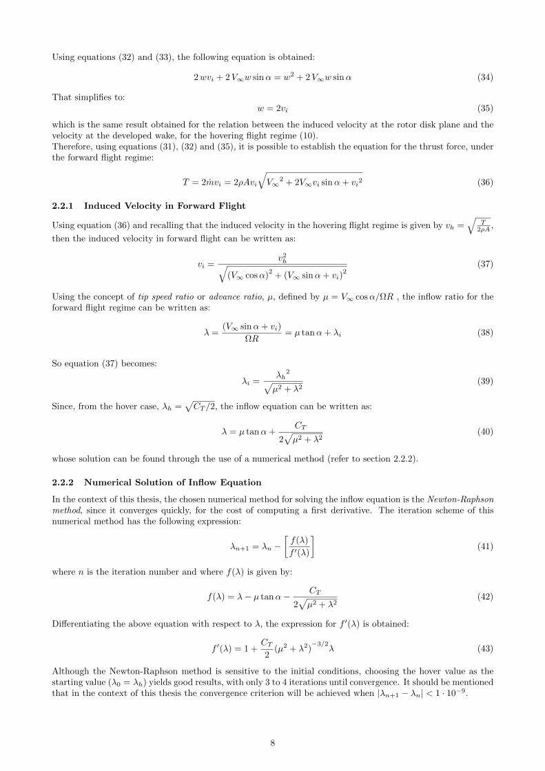
Using equations (32) and (33), the following equation is obtained:
2wvi + 2V∞w sinα = w2 + 2V∞w sinα (34)
That simplifies to:w = 2vi (35)
which is the same result obtained for the relation between the induced velocity at the rotor disk plane and thevelocity at the developed wake, for the hovering flight regime (10).Therefore, using equations (31), (32) and (35), it is possible to establish the equation for the thrust force, underthe forward flight regime:
T = 2mvi = 2ρAvi
√V∞
2 + 2V∞vi sinα+ vi2 (36)
2.2.1 Induced Velocity in Forward Flight
Using equation (36) and recalling that the induced velocity in the hovering flight regime is given by vh =√
T2ρA ,
then the induced velocity in forward flight can be written as:
vi =v2h√
(V∞ cosα)2
+ (V∞ sinα+ vi)2
(37)
Using the concept of tip speed ratio or advance ratio, µ, defined by µ = V∞ cosα/ΩR , the inflow ratio for theforward flight regime can be written as:
λ =(V∞ sinα+ vi)
ΩR= µ tanα+ λi (38)
So equation (37) becomes:
λi =λh
2√µ2 + λ2
(39)
Since, from the hover case, λh =√CT /2, the inflow equation can be written as:
λ = µ tanα+CT
2√µ2 + λ2
(40)
whose solution can be found through the use of a numerical method (refer to section 2.2.2).
2.2.2 Numerical Solution of Inflow Equation
In the context of this thesis, the chosen numerical method for solving the inflow equation is the Newton-Raphsonmethod, since it converges quickly, for the cost of computing a first derivative. The iteration scheme of thisnumerical method has the following expression:
λn+1 = λn −[f(λ)
f ′(λ)
](41)
where n is the iteration number and where f(λ) is given by:
f(λ) = λ− µ tanα− CT
2√µ2 + λ2
(42)
Differentiating the above equation with respect to λ, the expression for f ′(λ) is obtained:
f ′(λ) = 1 +CT2
(µ2 + λ2)−3/2
λ (43)
Although the Newton-Raphson method is sensitive to the initial conditions, choosing the hover value as thestarting value (λ0 = λh) yields good results, with only 3 to 4 iterations until convergence. It should be mentionedthat in the context of this thesis the convergence criterion will be achieved when |λn+1 − λn| < 1 · 10−9.
8
2.2.3 Total Power Equation in Forward Flight
Based on [6] and having selected an approach to compute the solution of the inflow equation, it is possible towrite the final equation that will predict the total rotor power requirements in the forward flight regime. Asseen before, the total power requirements will be the sum of the induced power component with the profilepower component generated by the rotor.
Recalling that the induced power is given by Tvi (or in the non dimensionalized form CTλi), and using theequation (39), the induced power coefficient can be written as:
CPi = CTλi =C2T
2√µ2 + λ2
(44)
However, as analyzed in the hover case, the non-ideal effects are not being considered in the above equation. Toinclude this effects, the induced power correction factor must be taken in account. Hence the corrected equationfor the induced power coefficient in the forward flight regime is:
CPi = k CTλi =k C2
T
2√µ2 + λ2
(45)
Regarding the profile power generated by the rotor, the same strip analysis used for the hover case will beemployed in the forward case. Nonetheless, since in the forward flight regime there is an additional translationalcomponent of velocity (V∞), its effects must be accounted in the profile drag estimation. This influence wasfirst suggested by [11] and can be approximated as:
CP0=σCd0
8(1 +Kµ2) (46)
where the numerical value of K varies from 4.5 in hover to 5 at µ = 0.5, depending on the various assumptionsthat are made.
Having established the expressions for each component contributing to the total power requirements, the totalpower coefficient in the forward flight regime can be written as:
CP =k C2
T
2√µ2 + λ2
+σCd0
8(1 +Kµ2) (47)
It should be noted that when considering that µ = 0 in the above equation, meaning that the helicopter is inthe hover regime, the result obtained is identical to the one derived for the hover case (equation (29)). This isa crucial result and shows that equation (47) can be used as a general equation for the prediction of the totalpower requirements.
2.2.4 Extension of Momentum Theory to other Rotor Systems
Momentum Theory analysis can also be extended for other helicopter rotor designs, including contrarotatingCo-Axial and Tandem systems and this will be discussed in the following sections.
Co-Axial SystemsThe advantage of using an helicopter with a coaxial rotor configuration is that the net size of the rotors is re-duced, since each rotor now produces vertical thrust. In addition, no tail rotor is required for counterbalancingthe torque produced by the main rotor, so all power can be devoted to useful lift generation. However, sincethe wake of the two rotors interfere with each other, this flow interaction will result in a loss of the net rotorsystem aerodynamic efficiency.
According to [6] and considering a simple momentum analysis of the coaxial rotor, in hovering flight, andassuming that the rotor planes are sufficiently close together and that each rotor disk plane provides a thrustequal to half the total helicopter weight (T = W/2), the induced velocity of the rotor system, will be given by:
vi =
√2T
2ρA(48)
Therefore the induced power is:
Pi = 2Tvi =(2T )
3/2
√2 ρA
(49)
9

However, considering each rotor separately, the induced power of the two rotors is given by:
Pi =2(T )
3/2
√2 ρA
(50)
So defining the interfering power factor, kint as the ratio between equation (49) and (50) then:
kint =
(2T )3/2
√2 ρA
2(T )3/2
√2 ρA
=√
2 (51)
which shows that the induced power of a coaxial rotor system is 41% bigger than the power required to operatetwo rotors in isolation. This simple momentum analysis of the problem, when compared with experimentalmeasurements, has been shown to be overly pessimistic. The main reason for the over estimation of the inducedpower is related to the finite spacing that exists between the two rotors. Generally for co-axial rotor systems, therotors are designed in such a way that the rotors are spaced sufficiently far apart that the lower rotor operatesin the fully developed wake of the upper rotor (figure 5).
Figure 5: Flow model for co-axial rotor analysis ([6], pg. 102)
To tackle this problem and assuming that the lower rotor does not influence the upper rotor performance, theinduced velocity at the upper rotor is given by:
vu =
√T
2ρA= vh (52)
Considering that the fully developed wake of the upper rotor has an area equal to A/2 and a flow velocity of2vu, there will be, over the inner half of the lower rotor plane, a velocity of 2vu + vi, over the outer half of thelower disk area, a velocity of vl and in the fully developed wake of the lower rotor, a velocity given by wl.So, applying the principle of mass conservation on the lower rotor plane, the following yields:
m = ρA
2(2vu + vl) + ρ
A
2vl = ρA(vu + vl) (53)
Applying now the principle of conservation of momentum, on the plane of the fully developed wake, the thruston the lower rotor plane is given by:
Tl = ρA(vu + vl)wl − 2ρAvu2 (54)
10

and the work done by the lower rotor:Pl = Tl(vu + vl) (55)
which will be equal to the gian in kinetic energy of the slipstream. Therefore:
Tl(vu + vl) = ρA(vu + vl)wl2 − 1
2ρ
(A
2
)(2vu)(2vu)2 =
1
2ρA(vu + vl)wl
2 − 2ρAvu3 (56)
Assuming that Tl = Tu = T , then T = 2ρAvu2 and using equation (54):
Tl = T =1
2ρA(vu + vl)wl (57)
that together with equation (56) gives:
T (2vu + vl) =1
2ρA(vu + vl)wl
2 (58)
Using equations (57) and (58), it yields wl = 2vu+vl and substituting this into equation (57) and recalling thatT = 2ρAvu
2, it yields:4ρAv2
u = ρA(vu + vl)wl = ρA(vu + vl)(2vu + vl) (59)
Rearranging equation (59) and solving in terms of vl gives:
vl =
(−3 +
√17
2
)vu = 0.5616vu (60)
Finally, since the power of the upper rotor is Pu = Tvu = Tvh and that the power for the lower rotor isPl = T (vu + vl), the total power of the co-axial rotor system is given by 2.5616Tvh. Comparing this with tothe total power of the rotors operating in isolation, 2Tvh, the interference power factor is then given by:
kint =(Pi)coaxial
(2Pi)isolated=
2.5616Tvh2Tvh
= 1.281 (61)
which translates in a 28% increase in total induced power required compared to the 41% obtained with theprevious analysis and is closer to the experimental values, for which kint ≈ 1.16.
Having established the induced power estimation, it is now possible to write the expression that computesthe total power needs of a contra-rotating co-axial rotor systems, in hovering flight, which is given by:
P =kint k(2T )3/2
√4ρA
+ ρA(ΩR)3
(2σCd0
8
)(62)
where the factor 2 in the profile power expression, accounts for profile power generated by the presence of asecond rotor in the system.It should be noted that when using k = 1.15 and kint = 1.16, there is a good agreement between momentumtheory and the measured data that confirms that the coaxial rotor can be analyzed as two rotors operatingisolatedly but with an interference effect, accounted by kint.
Regarding the forward flight regime, an identical analysis will be considered. Applying the concept of theinterference factor (where the same value of kint is assumed for both rotors and is independent of the forwardvelocity), the non-dimensionalized form of the total power requirements, for forward flight, can be written as:
CP =2kintk C
2T
2√µ2 + λ2
+2σCd0
8(1 +Kµ2) (63)
It should be mentioned, as previously seen, that when considering µ = 0 in the above equation, the resultobtained will be identical to equation (62). This proves that equation (63) is a general equation and can beused for the the hover and forward flight regimes.
Tandem SystemsTandem rotor designs are used most commonly used for heavy-lift helicopters because, like the coaxial design,all of the rotor power is used to generate useful lift. However the induced power of a partly overlapping tandemrotor system is higher than that of the two isolated rotors, since one of the rotors will operate in the slipstreamof the other rotor, resulting in a higher induced power, for the same thrust produced.
11

Figure 6: Flow models used for tandem configuration analysis ([6], pg. 107)
According to [6], the Momentum Theory analysis of overlapping rotors is based on the concept of overlappingareas (figure 6). Assuming Aov = mA as the overlap area (figure 6) and that the rotors have no vertical spacing,by means of geometry it can be shown that:
m′ =AovA
=2
π
[θ − d
Dsin θ
], (64)
where θ = cos−1 ( dD ). If T1 and T2 are the thrust forces produced by each rotor (which may be unequal), thethrust produced on the overlapping region is given by m(T1 + T2). Based on the uniform inflow assumptions,then the induced power consumed by each of the areas (area 1, area 2 and the overlapping area) is:
P1 =(1−m′)T1
3/2
√2ρA
, P2 =(1−m′)T2
3/2
√2ρA
, and Pov =m′(T1 + T2)3/2
√2ρA
(65)
and the total power is given by Ptotal = P1 +P2 +Pov. So, defining the interference power factor, kov (similarlyto what was done for the co-axial case), as the ratio between the induced power required by the tandem rotorsystem and the one required by two isolated rotors, it yields:
kov =PitotalPiisolated
=(1−m′)T1
3/2 + (1−m′)T23/2 +m′(T1 + T2)3/2
T13/2 + T2
3/2(66)
If it is assumed that each rotor produces the same thrust, T1 = T2, equation (66) reduces to:
kov = 1 + 0.4141m′ (67)
Based on [12], an alternative approximation to kov, is:
kov ≈
[√
2−√
2
2
d
D+
(1−√
2
2
)(d
D
)2]
(68)
The dependency of kov on rotor overlap has been measured experimentally using subscale rotor models, andit is apparent that the momentum theory produces a good agreement with the measurements, although theapproximate result given by equation (68) underpredicts the kov value, and the amount of data available isrelatively scarce when compared to single rotor data (figure 7).Having established the induced power estimation, it is now possible to write the expression that computes thetotal power needs of a tandem rotor system, in hovering flight, which is given by:
P =kov k(2T )3/2
√4ρA
+ ρA(ΩR)3
(2σCd0
8
)(69)
12

Figure 7: Tandem rotor overlap induced power correction in hover as derived from momentum theory andcompared to measurements ([6], pg. 106)
Regarding the forward flight regime, an identical analysis will be considered. Applying the concept of theoverlapping factor (where the same value of kov is assumed for both rotors and is independent of the forwardvelocity) and recalling equation (47), the non-dimensionalized form of the total power requirements, for forwardflight, can be written as:
CP =2kovk C
2T
2√µ2 + λ2
+2σCd0
8(1 +Kµ2) (70)
However, the analysis of measured data of the forward flight performance obtained shows that for µ > 0.1, theperformance of the the front rotor was almost identical of that of a single isolated rotor, suggesting that in thiscase there is little or no interference produced on the forward rotor by the rear rotor. Therefore, the powerrequired for the rear rotor is considerably higher because it operates in the downwash generated by the frontrotor. With this considerations and applying the overlapping factor, kov, the induced power for the tandemconfiguration is:
Pi = Tfvif + kovTrvir = Tfvi + kovTrvi (71)
So the total rotor power of a tandem configuration system, in the non dimensionalized form, through MomentumTheory analysis, in the forward flight regime for which µ > 0.1 can be written as:
CP =k C2
T
2√µ2 + λ2
+kovk C
2T
2√µ2 + λ2
+2σCd0
8(1 +Kµ2) (72)
2.3 Blade Element Analysis in Hovering Flight
The Blade Element Theory (BET) forms the basis of the most modern analysis of helicopter rotor aerodynam-ics because it provides an estimation of the local radial and azimuthal distributions of the blade aerodynamicloading over the rotor disk, in contrast with Momentum Theory, which is a global analysis [13]. BET was firstdesigned by [14], and [15] to determine the behavior of airplane propellers, and assumes that each blade sectionacts as a 2-D airfoil to produce aerodynamic loads. The overall rotor performance can be obtained by integrat-ing the sectional aerodynamics forces (and moments), at each blade element over the length of the blade andaveraging the result over a rotor revolution. Therefore, since BET relates the overall rotor performance withdetailed design parameters, it can be used as basis to design the rotor blades in terms of blade twist, planformdistribution and the airfoil shape.
Blade Element Analysis in Hover FlightFigure 8 depicts the flow environment and aerodynamic forces at a representative blade element, in which theaerodynamic loads are assumed to arise solely from the velocity and the AoA normal to the leading edge of theblade section.
13

Figure 8: Incident velocties and aerodynamic environment at a typical blade element([6], pg. 116)
Based on [6], the resultant local flow velocity at any blade element at a radial distance y from the rotationalaxis, has an out-of plane component UP = Vc + vi, which is normal to the rotor, due to the induced inflow andthe climb velocity (in case there is one) and an in-plane component UT = Ωy, parallel to the rotor due to bladerotation. Therefore, the resultant velocity at a blade element can be written as:
U =√U2T + U2
P (73)
and the relative inflow angle:
φ = tan−1
(UPUT
)(74)
Defining θ as the blade element pitch angle, the effective angle of attack is given by:
α = θ − φ = θ − tan−1
(UPUT
)(75)
Regarding the resultant incremental lift and drag, per unit span, at each blade element they can be written as:
dL =1
2ρU2cCldy, (76)
dD =1
2ρU2cCddy (77)
where Cl and Cd are the lift and drag coefficients. The incremental lift and drag forces act, respectively,perpendicular and parallel to the resultant flow velocity. Based on Figure 8 these forces can be resolvedperpendicular (z) and parallel (x) to the rotor disk plane, yielding:
dFz = dL cosφ− dD sinφ (78)
dFx = dL sinφ+ dD cosφ (79)
Therefore, the incremental thrust, torque and power of the rotor are:
dT = NbdFz, (80)
14

dQ = NbdFxy, (81)
dP = NbdFxΩy (82)
Substituting the results for dFx and dFz gives:
dT = Nb(dL cosφ− dD sinφ), (83)
dQ = Nb(dL sinφ+ dD cosφ)y, (84)
dP = Nb(dL sinφ+ dD cosφ)Ωy (85)
In helicopter aerodynamics the out of plane velocity Up can be considered to be much smaller that the in-plane
velocity, UT , so one can write U =√U2T + U2
P ≈ UT .
Using this assumption and applying equations (76) and (77) into equations (80), (81) and (82), the followingis obtained:
dT = Nb
(1
2ρU2
T c
)[Cl cos
(tan−1
(UPUT
))− Cd sin
(tan−1
(UPUT
))]dy (86)
dQ = Nb
(1
2ρU2
T c
)[Cl sin
(tan−1
(UPUT
))+ Cd cos
(tan−1
(UPUT
))]y dy (87)
dP = Nb
(1
2ρU2
T c
)[Cl sin
(tan−1
(UPUT
))+ Cd cos
(tan−1
(UPUT
))]Ω y dy (88)
At this stage it is convenient to introduce nondimensional quantities by dividing lengths by R and velocities bythe rotational tip speed, ΩR. Hence:
r =y
R(89)
UTΩR
=Ωy
ΩR=y
R= r (90)
and:
λ =Vc + vi
ΩR=
(Vc + vi
Ωy
)(Ωy
ΩR
)=UPUT
( yR
)= tan(φ) r (91)
Therefore the incremental thrust coefficient can be written as:
dCT =Nb(
12ρU
2T c) [Cl cos
(tan−1
(λr
))− Cd sin
(tan−1
(λr
))]dy
ρA(ΩR)2= (92)
dCT =Nb(
12ρ (Ωy)2 c
) [Cl cos
(tan−1
(λr
))− Cd sin
(tan−1
(λr
))]dy
ρ(πR2)(ΩR)2= (93)
dCT =1
2
(Nbc
πR
)[Cl cos
(tan−1
(λ
r
))− Cd sin
(tan−1
(λ
r
))] ( yR
)2
d( yR
)= (94)
dCT =1
2σ
[Cl cos
(tan−1
(λ
r
))− Cd sin
(tan−1
(λ
r
))]r2dr (95)
Equation (95) is one of the most fundamental equations for any rotating-wing analysis. Similarly, the incrementalpower an torque coefficients are given by:
dCP =Nb(
12ρU
2T c) [Cl sin
(tan−1
(λr
))+ Cd cos
(tan−1
(λr
))]Ωy dy
ρA(ΩR)3= (96)
dCP =Nb(
12ρ (Ωy)2 c
) [Cl sin
(tan−1
(λr
))+ Cd cos
(tan−1
(λr
))]Ωy dy
ρ(πR2)(ΩR)3= (97)
dCP =1
2
(Nbc
πR
)[Cl sin
(tan−1
(λ
r
))+ Cd cos
(tan−1
(λ
r
))] ( yR
)3
d( yR
)= (98)
dCP =1
2σ
[Cl sin
(tan−1
(λ
r
))+ Cd cos
(tan−1
(λ
r
))]r3dr (99)
15

which represents the sum of the induced power and the profile power required.
2.3.1 Rotor Thrust and Power estimation in Hover
To find the total CT , CQ and CP the incremental thrust, torque and power coefficients must be integrated alongthe the blade, in the spanwise direction. Therefore, for a general blade shape and configuration, the thrustcoefficient is given by:
CT =1
2
∫ 1
0
σ(r)
[Cl cos
(tan−1
(λ(r)
r
))− Cd sin
(tan−1
(λ(r)
r
))]r2dr (100)
where the limits of integrating are r = 0 and r = 1, corresponding to the blade root and tip, respectively. Forthe power and torque coefficients it yields:
CQ = CP =1
2
∫ 1
0
σ(r)
[Cl sin
(tan−1
(λ(r)
r
))+ Cd cos
(tan−1
(λ(r)
r
))]r3dr (101)
It should be noted that in order to evaluate CT and CP it is necessary to predict the spanwise variation ofthe inflow ratio, λ(r), the sectional aerodynamic force coefficients, Cl and Cd, and also the spanwise chord
distribuition since, σ(r) = Nbc(r)πR . If 2-D aerodynamics are assumed, then the sectional lift and drag coeffi-
cients will be a function of the local effective angle of attack and of the local Reynolds and Mach numbers(Cl = Cl(α,Re,M) and Cd = Cd(α,Re,M)). Also, the effective angle of attack will depend on the induced andclimb velocities, as well on the pitch angle (α = α(Vc, θ, vi)) and lastly, the induced velocity will be function ofthe spanwise position along the blade(vi = vi(r)). Since these effects cannot, in general, be explicitly expressedin an analytic form, it will be necessary to numerically solve the integrals for CT , CQ and CP .
2.4 Blade Element Analysis in Forward Flight
The same blade element assumptions and approximations previously used for the hovering flight can alsobe considered valid for forward flight [6]. As before, the velocity at a blade element is decomposed in anperpendicular velocity component, UP and a tangential component, UT , perpendicular to the leading edge ofthe blade. However, in forward flight, the velocity components are periodic at the the rotor rotational frequencyand depend on the blade azimuthal position (ψ).
Figure 9: Perturbation velocties on the blade resulting from blade flapping velocity and rotor coning ([6], pg.157)
For the in-plane velocity, and comparing with the hover case, there is now a further free stream (translational)velocity component, such that:
UT = Ωy + V∞ sinψ (102)
Regarding the out-of-plane component, there is now two more terms that result from perturbations producedby the flapping motion of the blade. The term yβ is result of the blade flapping velocity and µΩRβ(ψ) cos(ψ)is produced due to the blade flapping displacements (figure 9). So, the velocity perpendicular to the rotor disk,can be written as:
UP = (Vc + vi) + yβ(ψ) + V∞β(ψ) cos(ψ) (103)
In forward flight, there is also a radial velocity component, parallel to the span axis of the blade, which is givenby:
UR = µRΩ cosψ (104)
16

However, in BET, the aerodynamics effects produced by the radial velocity component and by the termsdepending on the coning angle and on the coning angle time variation are neglected and will not be consideredin the context of this thesis.Hence, in the forward flight regime, the expressions that will be used for each velocity component throughoutthis thesis are:
UT = Ωy + V∞ sinψ (105)
UP = Vc + vi (106)
UR = 0 (107)
2.4.1 Rotor Thrust and Power estimation in Forward flight
To estimate the total thrust, power and torque coefficients required in the forward flight regime, the procedurewill be almost identical to the one adopted in the hover case. Firstly, the incremental thrust, power and torquecoefficients will be defined, and after, they will be integrated along the blade spanwise direction.
Since the approximation U =√U2P + U2
T remains valid in the forward flight regime, the general expressions forthe incremental thrust, torque and power will be similar to the ones obtained for the hover case. Therefore,based on [6], the incremental quantities can be written as:
dT = Nb
(1
2ρU2
T c
)[Cl cos
(tan−1
(UPUT
))− Cd sin
(tan−1
(UPUT
))]dy (108)
dQ = Nb
(1
2ρU2
T c
)[Cl sin
(tan−1
(UPUT
))+ Cd cos
(tan−1
(UPUT
))]y dy (109)
dP = Nb
(1
2ρU2
T c
)[Cl sin
(tan−1
(UPUT
))+ Cd cos
(tan−1
(UPUT
))]Ω y dy (110)
At this stage, similarly to what was previously done for the hover case, it is convenient to introduce nondimensional quantities. Hence:
r =y
R(111)
UTΩR
=Ωy + V∞ sinψ
ΩR= r + µ sinψ (112)
and:
λ =Vc + vi
ΩR=
(Vc + vi
Ωy + V∞ sinψ
)(Ωy + V∞ sinψ
ΩR
)=UPUT
(r + µ sinψ) = tan(φ) (r + µ sinψ) (113)
Applying the results obtained above, the incremental thrust coefficient can be written as:
dCT =Nb(
12ρU
2T c)
[Cl sinφ− Cd cosφ] dy
ρA(ΩR)2= (114)
dCT =Nb(
12ρ (Ωy + V∞ sinψ)2 c
)[Cl sinφ− Cd cosφ] dy
ρ(πR2)(ΩR)2= (115)
dCT =1
2
(Nbc
πR
)[Cl sinφ− Cd cosφ]
(Ωy + V∞ sinψ
ΩR
)2
d( yR
)= (116)
dCT =1
2σ [Cl sinφ− Cd cosφ] (r + µ sinψ)2dr (117)
Similarly the incremental power and torque coefficients are given by:
dCP =Nb(
12ρU
2T c)
[Cl sinφ+ Cd cosφ] (Ωy + V∞ sinψ) dy
ρA(ΩR)3= (118)
dCP =Nb(
12ρ (Ωy + V∞ sinψ)2 c
)[Cl sinφ+ Cd cosφ] (Ωy + V∞ sinψ) dy
ρ(πR2)(ΩR)3= (119)
dCP =1
2
(Nbc
πR
)[Cl sinφ+ Cd cosφ]
(Ωy + V∞ sinψ
ΩR
)3
d( yR
)= (120)
dCP =1
2σ [Cl sinφ+ Cd cosφ] (r + µ sinψ)3 dr (121)
17

To find the total CT , CQ and CP , the incremental thrust, torque and power coefficients must be integrated alongthe the blade, in the spanwise direction. Since in forward flight the velocity field, depends on the blade azimuthalposition, a second integration in ψ is also required. Therefore, for a general blade shape and configuration, thetotal thrust coefficient is given by:
CT =1
4π
∫ 2π
0
∫ 1
0
σ(r)
[Cl cos
(tan−1
(λ(r, ψ, µ)
r + µ sinψ
))− Cd sin
(tan−1
(λ(r, ψ, µ)
r + µ sinψ
))](r + µ sinψ)2 dr dψ
(122)and for the power and torque coefficients it yields:
CQ = CP =1
4π
∫ 2π
0
∫ 1
0
σ(r)
[Cl sin
(tan−1
(λ(r, ψ, µ)
r + µ sinψ
))+ Cd cos
(tan−1
(λ(r, ψ, µ)
r + µ sinψ
))](r+µ sinψ)3 dr dψ
(123)Similarly to the hover case, in order to evaluate CT and CP it is necessary to predict, the sectional aerodynamicforce coefficients, Cl and Cd, the spanwise chord distribuition, c(r) and the spanwise azimuthal and spanwisevariation of the inflow ratio, λ(r, ψ, µ). Also, the same 2-D aerodynamics and dependencies will be assumed.However, since the axissymetry of the inflow is lost in the forward flight regime, the estimation of the spanwisevariation of the inflow ratio, is not as straightforward as in the hover case and will require a detailed analysis,which will be done in the following section.
2.4.2 Linear Inflow models
The induced velocity field, in the forward flght regime, depends on the knowledge of the rotor wake, which inturn depends on the rotor thrust, on the overall blade colective and cyclic pitch angles and on the distributionof airloads over the blades. Also, the effects of indiviual tip vortices tend to produce a highly non uniform inflowdistribution. To incorporate all this effects in calculations would be an undertaking challenge. Nevertheless,the performance of the rotor can be analyzed using simpler models that represent the basic effects resultingfrom the rotor wake. These models are called inflow models and were formulated on the basis of experimentalresults and measured data. Because of their simplicity, inflow models have found great utility in helicopter rotoraerodynamics.The first in flight experiment to measure the time-average-induced velocity over the rotor disk in forward flightwas made by [16]. Based on measurements of angular displacements of smoke streamers, the longitudinalinflow variation was determined to be approximately linear. Since then various experiments confirmed theapproximately linear longitudinal variation of in the inflow and its complicated nature, since there is a transitionregion within the range 0.0 ≤ µ ≤ 0.1, in which the induced velocity in the plane of the rotor is the most uniform,strongly affected by the presence of discrete tip vortices. However in higher speed forward flight (µ ≥ 0.15) theinflow distribution becomes approximately linear and can be represented by:
λi = λ0(1 + kxx
R) = λ0(1 + kxr cosψ) (124)
which is a form suggested by [11]. The coefficient λ0 is the average induced velocity at the center of the rotorand is given by the Momentum Theory:
λ0 =CT
2√µ2 + λ2
i
(125)
where kx = 1.2 , which means that there is a small upwash at the leading edge of the rotor and an increase indownwash relative to the average value along the trailing edge (figure 10).
18

Figure 10: Linear inflow model approximation over the rotor disk ([6], pg. 159)
A variation of this result is to consider both a longitudinal and lateral variation of the inflow distribution. Inthis case:
λi = λ0(1 + kxx
R+ ky
y
R) = λ0(1 + kxr cosψ + kyr sinψ) (126)
where kx and ky can be viewed as weighting factors and represent the deviation of the inflow from the valuepredicted by Momentum Theory. Various attempts have been made to directly estimate kx and ky. Using rigidcylindrical vortex wake theories [17] suggested for kx:
kx = tan(χ
2
)(127)
where the wake skew angle is defined by:
χ = tan−1
(µx
µz + λi
)(128)
and where µx and µz are the advance ratios parallel and perpendicular to the rotor disk. It should be noticedthat the apparent skew angle increases rapidly with the advance ratio and that for µ > 0.2, the wake isapproximately flat (figure 11). Also for high speed forward flight kx ≈ 1, which doesn’t represent the smallregion of upwash usually measured at the leading edge of the disk. Another linear inflow model commonlyemployed in basic rotor analysis was suggested by [18]. In this model, kx and ky are obtained with anothervariation of the vortex theory and are given by:
kx =4
3
(1− cosχ− 1.8µ2
sinχ
), ky = −2µ (129)
yielding kx = 0 for µ = 0, and has a maximum value of 1.11 at µ ≈ 0.2, slowly decreasing thereafter. Drees’smodel is easy to implement in rotor analysis and gives a good description of the rotor inflow.Several other models to estimate the values of kx and ky were developed by different authors and are summarizedin table 1:
Author(s) kx kyColeman et al. (1945) tan(χ/2) 0Drees (1949) (4/3)(1− cosχ− 1.8µ2)/ sin(χ) −2µPayne (1959) (4/3)[µ/λ/(1.2 + µ/λ)]) 0
White&Blake (1979)√
2 sinχ 0Pitt&Peters (181) (15π/23) tan(χ/2) 0Howlett (1981) sin(χ)2 0
Table 1: Various estimated values of first harmonic inflow ([6], pg. 160)
Similarly to what has been considered for the Momentum Theory analysis in the forward flight regime, theinflow equation, in the context of this thesis, will be solved through the use of Newton-Raphson numericalmethod.
19

Figure 11: Typical variation in rotor wake skew angle with thrust and advance ratio ([6], pg. 160)
2.4.3 Extension of Blade Element Theory to other Rotor Systems
The performance of the co-axial and tandem rotor systems have been previously discussed in the MomentumTheory section. It has been shown that by accounting the induced interference effects between the rotors byapplying an interference factor on the equations for each configuration, will yield considerably good results(figure 12 and 13). The same procedure will be used in the Blade Element Theory analysis of the co-axial andtandem rotor system configuration.
Co-Axial ConfigurationBased on [6] and considering the above assumptions and applying the interference power factor, kint, on equa-tion (123), the general power coefficient equation for the co-axial configuration, in the hover and forward flightregime, using the Blade Element Theory can be written as:
CP =
∫ 2π
0
∫ 1
0
σ(r)
4π
[2 kint Cl(r) sin
(tan−1
(λ(r)
r + µ sinψ
))+ 2Cd(r) cos
(tan−1
(λ(r)
r + µ sinψ
))](r+µ sinψ)3 dr dψ
(130)
where the factor 2, applied in each power term, accounts for the induced and profile power generated bythe presence of two rotors.
Tandem ConfigurationFor the tandem rotor system analysis through Blade Element Theory in the hover flight regime, consideringthat each rotor will contribute to the profile power generation, and that each rotor produces the induced powerof a single isolated rotor multiplied by the overlapping power factor, kov, the following is obtained:
CP =1
4π
∫ 1
0
σ(r)
[2 kov Cl(r) sin
(tan−1
(λ(r)
r + µ sinψ
))+ 2Cd(r) cos
(tan−1
(λ(r)
r + µ sinψ
))]r3dr (131)
Recalling the analysis made in section 2.2.4 in which the measured data showed that for value of µ > 0.1, theperformance of the the front rotor was almost identical of that of a single isolated rotor and that the rear rotoroperated in the downwash of the front rotor, the induced power for the tandem configuration is:
Pi = Tfvif + kovTrvir = Tfvi + kovTrvi (132)
So the total rotor power of a tandem configuration system, in the non dimensionalized form, through BladeElement theory analysis, in the forward flight regime for which µ > 0.1 can be written as:
CP =
∫ 2π
0
∫ 1
0
σ(r)
4π
[(1 + kov)Cl(r) sin
(tan−1
(λ(r)
r + µ sinψ
))+ 2Cd(r) cos
(tan−1
(λ(r)
r + µ sinψ
))](r+µ sinψ)3 dr dψ
(133)
20

Figure 12: Prediction of power in forward flight for single and coaxial rotor system compared to measurements([6], pg. 241)
Figure 13: Prediction of power in forward flight for a tandem rotor system compared to measurements ([6], pg.242)
2.5 Helicopter Performance
The aerodynamic tools described in the previous sections to analyze the behavior of rotor systems, can now beused to study the basic performance of the helicopter. This analysis will include the estimation of the powerrequired for a given flight condition and an estimation of the helicopter endurance and range.
2.5.1 Density
An important point that must be taken into account is that the performance of the helicopter as a whole is afunction of the air density.In the lower atmosphere, where the helicopters commonly fly (below 6000m), the standard value of air densitycan be closely approximated based on [6], by the equation:
ρ
ρ0= exp
(−0.0296h
304.8
)(134)
where h is expressed in meters and ρ0 = 1.225 kg/m3, which is the standard density value at sea level (h = 0).
21

2.5.2 Parasitic Power in Forward Flight
Figure 14: Equilibrium of forces on a helicopter in forward flight ([6], pg. 218)
According to [6], the equilibrium of forces on a single rotor helicopter in a horizontal forward flight situationcan be depicted as show in Figure 14. For the vertical equilibrium of forces, the following can be written:
T cos(αTPP ) = W (135)
and to satisfy the horizontal equilibrium:T sin(αTPP ) = D (136)
Rearranging and solving for the disk AoA, yields:
αTPP = tan−1
(D
W
)(137)
Now considering that the power to propel the helicopter forward is given by TV∞ sin (αTPP ) and using thesmall angle approximations, the following equation is obtained:
PP = TV∞ sin (αTPP ) =W
cos (αTPP )V∞ sin
[tan−1
(D
W
)]≈WV∞
D
W= DV∞ (138)
This power term is known as Parasitic Power and represents the energy lost due to viscous effects. This is aresult of the viscous shear effects and flow separation (Pressure Drag) on the airframe, rotor hub and on theother helicopter core components. Because helicopter airframes are much less aerodynamic that their fixed-wingcounterparts, this source of drag can be very significant and cannot be disregarded.
Although equation (138) is a very straightforward approach, an alternative method to estimate the parasiticpower requirements, is often used in helicopter analysis. Rewriting equation (138) as:
PP =
(1
2ρV 2∞SrefCDf
)V∞ (139)
where Sref is some reference area and CDf is the drag coefficient based on this area. In the non dimensionalizedform, it can be written as:
CPP =1
2
(SrefA
)µ3CDf =
1
2
(f
A
)µ3 (140)
where A is the rotor disk area and f (= CDfSref ) is known as the equivalent flat plate area and accounts mainlyfor the drag of the hub, fuselage and landing gear. The need of this parameter comes from noting that in theconventional form the drag coefficient can be written as:
CDf =Df
12ρV
2∞Sref
(141)
22

in which the definition of Sref may not be unique. Thus, an equivalent wetted area is used, which is defined by:
f =Df
12ρV
2∞
(142)
and avoids any confusion that may arise from the ambiguous definition of Sref .
It should be noted that the parasitic power term will be summed to all the total power requirements equa-tions established and defined in the Momentum Theory and Blade Element Theory sections.
2.5.3 Tip Losses Estimation
Based on [6], an important non-ideal effect, whose analysis must also be taken in account, is the tip lossesphenomenon. The formation of trailed vortex at the tip of each blade produces a local inflow over the tip regionthat reduces effectively the lift generation capability over the tip region.
For a preliminary rotor design work, a simple tip-loss factor B can be used to account for this physical ef-fect such that the product BR represents a reduction in the rotor lift generating blade radius that translates toa reduction by a factor of B2 of the rotor effective (lift generating) disk area (figure 15). Therefore this effectwill manifest as a higher disk loading (i.e. T
Aeinstead of T
A ) and an increase of the induced velocity by a factor
of B−1, with a corresponding increase in the induced power.
One of the first approaches to estimate the tip loss is given by the following expression [6]:
B = 1− 1.386
Nb
λi√λi
2 + 1(143)
In helicopter rotors the value of λi is typically very small, thus equation above can be simplified to:
B = 1− 1.386
Nbλi (144)
For hovering flight, with the Momentum Theory based assumption of uniform inflow and using equation (22),it yields:
B = 1− 1.386√2
√CTNb
(145)
Another approach for modeling the tip loss effects was made by [23] who suggested an empirical tip loss factorbased only on the blade geometry, where:
B = 1− c
2R(146)
im which c is the tip chord. However this model would only produce satisfactory results for rectangular bladetip configurations. So [24] proposed the alternative geometric expression:
B = 1− c0(1 + 0.7τr)
1.5R(147)
where τr represents the ratio between the tip and root chords and c0 the tip chord.
23

Figure 15: Tip loss effect on blade tip ([6], pg. 75)
2.5.4 Tail Rotor Power
For a correct analysis of the total power requirements of the conventional helicopter configuration, the tail rotorpower cannon be disregarded. This power term typically varies between 3% and 5% of the power consumed bythe main rotor in normal flight, and can reach up to 20% at the extremes of the flight envelope. It is calculatedin a similar way to the main rotor power, with the thrust required being set equal to the value necessary tobalance the torque produced by the main rotor on the fuselage.
Considering xTR the distance between the main rotor shaft and the tail rotor shaft, the tail rotor thrustrequired is given by:
Ttr =(Pi + P0 + PP )
Ωxtr(148)
which in the non dimensionalized form can be written as:
CTtr =Ttr
ρAtrV 2tiptr
=Ttr
ρAtrΩ2trR
2tr
, (149)
Applying the general Momentum Theory equation for the conventional configuration to the tail rotor, the totaltail rotor power will be given by:
CPtr =k C2
Ttr
2√µ2 + λ2
tr
+σtrCd0tr
8(1 +Ktr µ
2) (150)
where σtr =NbtrctrπRtr
.
Regarding the Blade Element Theory analysis, and applying equation (123), the total tail rotor total power canbe written as:
CPtr =1
4π
∫ 2π
0
∫ 1
0
σtr(r)
[Cl(r) sin
(tan−1
(λtr(r)
r + µ sinψ
))+ Cd(r) cos
(tan−1
(λtr(r)
r + µ sinψ
))](r+µ sinψ)3 dr dψ
(151)It should be noted that for both theories the inflow velocity equation must be solved, applying the procedurethat was used for the main rotor in each theory, but taking in account the tail rotor characteristics, dimensionsand loads.
Having established the total tail rotor power requirements, this term will be summed to the total power equationof the conventional configuration defined by Momentum and Blade Element theories.
2.5.5 Climb Performance
The climb power requirements are equal to the time rate of increase of potential energy of the helicopter. Basedon [6] and assuming that the potential energy is denoted as E = Wh, the rate of increase of potential energy is
24

Wh = TVc = WVc, where W is the aircraft weight and Vc is the climb velocity.The general power equations defined before for each theory can be used to estimate the climb velocity Vc thatis possible at any given speed. Assuming that Pinst is the total power installed in the helicopter, the generalpower equation in the dimensional form can be written as:
Pinst = Pi + P0 + Pp + Pother + Pc (152)
where Pc = TVc, and where Pother includes the power terms that depend of the helicopter configuration (suchas the tail rotor power in the conventional configuration). Rearranging and solving in terms of Vc, the followingequation is obtained:
Vc =(Pinst − Pi + P0 + Pp + Pother)
T≈ (Pinst − Pi + P0 + Pp + Pother)
W(153)
It should be mentioned that since the power terms are function of the forward velocity V∞, the climb velocitywill also be dependent of the forward velocity. Therefore this equation must be solved for each value of V∞.
2.5.6 Maximum Endurance
Endurance is defined as the time that an helicopter is able to fly without refueling. To obtain the maximumendurance, the fuel burn per unit time must be a minimum. Considering that the weight of the fuel burn WF
in a given time t is given by:WF = SFC · P · t (154)
where SFC is the engine specific fuel consumption, the endurance can be written as:
t =WF
SFC · P(155)
Taking equation (155) into consideration, the maximum endurance will be obtained with the lowest SFC andlowest required power for flight. Since the SFC curve is fairly flat over the power spectrum analyzed in thecontext of this thesis, the endurance will be inversely proportional to the power required for flight. Thereforethe speed for maximum endurance coincides with the speed for minimum power.In the context of this thesis, the estimation of the speed of minimum power will be done by computing theminimum value of the total power curve obtained for each theory and configuration.
Although equation (155) yields an relatively accurate prediction of the endurance, it does not take in ac-count that the power required varies with gross weight. Because gross weight decreases as fuel is burned, thepower required also decreases. In order to include this effect and to be able to estimate an accurate predictionof the endurance, an numerical integration must be performed. Considering that the fuel burn WF with respectto endurance, E, can be written as:
dWF
dE= P · SFC (156)
The corrected endurance estimation will be given, based on [6], by the following numerical integration:
E =
∫ WGTOW−WF
WGTOW
1
P · SFCdW (157)
However, since the fuel weight is normally a small fraction of the total gross weight of the helicopter, WGTOW ,equation (157) can be evaluated fairly accurately at the point in cruise in which the aircraft weight is equal tothe initial gross weight minus half the initial fuel weight, WF . Therefore the corrected endurance estimationequation can be written as:
E ≈WF
[1
P · SFC
]WGTOW−Wf/2
(158)
Since equation (158) yields the most accurate results compared with the computational time required to performthe calculation, it will be the one used throughout this thesis.
2.5.7 Maximum Range
The range of the helicopter is the maximum distance it can fly for a given takeoff weight and for a given amountof fuel. The range can be written as Ra = V t so using the SFC concept and a given amount of fuel mass WF ,the following is obtained:
Ra =VWF
SFC · P(159)
25

Analyzing the above equation a first crude approximation to the speed of maximum range is obtained whenthe ratio V/P is maximum or the ratio P/V is minimum, that is, when the helicopter is operated at the bestlift-to-drag ratio [6]. Therefore the speed of maximum range, in non dimensional form, can be found by solvingthe following equation:
dCPdµ
= 0 (160)
Since in the context of this thesis the total power requirements curve will be estimated for each theory andconfiguration, the speed of maximum range can be computed by finding numerically the minimum of the curvedefined by the ratio between the total power requirements curve and the forward speed. This approach willspare the development of an analytically expression to compute the derivative of the general power curve withthe forward velocity.
However as considered in section 2.5.6, equation (159) does not take in account that the power required varieswith the gross weight. Applying the same considerations that the gross weight and the power required decreasesas fuel is burned, a more accurate prediction of the range will be obtained by integrating numerically the rangeequation. Therefore, the fuel burn, WF , with respect to the range, R, can be written as:
dWF
dRa=P · SFC
V(161)
Hence the corrected range estimation equation will be given by:
Ra =
∫ WGTOW−WF
WGTOW
V
P · SFCdW (162)
which, as previously seen in the section 2.5.6, can be accurately approximated by:
Ra ≈WF
[V
P · SFC
]WGTOW−Wf/2
(163)
2.5.8 Compressiblity Analysis
Very often, in helicopter rotors, when operating in high speed forward flight, the speed of the tip of the advancingblade exceeds the drag divergence Mach number of the airfoil section. When this occurs, compressibility effectscome into play and significantly change the flow characteristics and the overall rotor performance. Therefore,for an accurate power requirements prediction, an analysis of this effects cannot be disregarded.
Figure 16: The region of the disk where the blade section reaches high Mach numbers ([6], pg. 221)
Based on [6], the region of the rotor disk affected by compressibility effects is represented in Figure 16 and canbe defined by finding where the incident Mach number of the flow exceeds the drag divergence Mach number,Mdd. For an unswept blade, the incident Mach is given by:
Mr,ψ =ΩR
a(r + µ sinψ) = MΩR (r + µ sinψ) (164)
where a is the sonic velocity and MΩR is the Mach number of the blade tip in hover. Therefore the region ofthe disk affected by compresibility effects can be defined by:
MΩR (r + µ sinψ) ≥Mdd (165)
26

or:
r + µ sinψ ≥ Mdd
MΩR(166)
Hence, the azimuth angle for the onset of the compressibility affected zone can be obtained by setting r = 1,yielding:
ψ1 = sin−1
[1
µ
(Mdd
MΩR− 1
)](167)
The symmetry of the problem suggests that the tip section that leaves the compressibility affected zone isgiven by ψ2 = 180 − ψ1. Therefore, the non dimensional spanwise coordinate that defines the start of thecompressibility zone, can be written as:
rdd =Mdd
MΩR− µ sinψ (168)
Using Blade Element theory considerations, the increment in profile power associated with this region, will begiven by:
∆CPσ
=1
4π
∫ ψ2
ψ1
∫ 1
rdd
(r + µ sinψ)3 ∆Cd r dr dψ (169)
where ∆Cd is the extra drag on the blade section when it exceeds the drag divergence Mach number, Mdd.[25] suggested that for a NACA airfoil with a given Mdd, this extra drag component can be approximated by:
∆Cd(M) =
12.5(M −Mdd)
3, for M > Mdd.
0, otherwise.(170)
However, an effective solution to reduce the compressibility problems, is found by sweeping back the blade tip.The physical explanation behind this effect is related to the fact that the lift and drag generation is mainlyaffected by the velocity component that is normal to the leading edge of the blade. Therefore sweeping backthe the blade tip, will allow the rotor to attain an higher advance ratio before compressibility effeccts manifestas an increase in sectional drag and an increase in the net rotor power required. Defining Λ as the local sweepangle, the velocity component normal to the leading edge, Un, is given by:
Un = ΩR(r + µ sinψ) cos Λ (171)
The incident mach number Mr,ψ can then be written as:
Mr,ψ =ΩR
a(r + µ sinψ) cos Λ = MΩR(r + µ sinψ) cos Λ (172)
If, for a certain rotor, the design goal is to maintain the local Mach number below the drag divergence Machnumber of the blade tip airfoil section, and considering that the design point is the azimuth angle in which thetranslation velocity component is the highest, i.e. ψ = 90, the sweep angle required to avoid any compressibilityissue will be given by:
Λ = cos−1
(Mdd
MΩR(r + µ)
)(173)
2.5.9 Reverse Flow Analysis
According to [6], at higher rotor advance ratios, a considerable amount of reverse flow will exist on the retreatingside of the rotor disk, meaning that the blade sections operate with the trailing edge into the relative wind.Starting by defining that the frontier of this region is given by the locus of points that satisfy UT = 0, thefollowing equation is obtained:
UT = 0 = ΩR(r + µ sinψ) (174)
The solution to this equation is given by r = −µ sinψ. Therefore the region of reverse flow where UT ≤ 0 isdefined by a circular shaped region centered at (r, ψ) = (µ/2, 270) with diameter µ (figure 17). In this reverseflow region the sign of both UT and the sectional drag contribution changes, and this must be taken in accountwhen performing the radial and azimuthal integration to find the rotor power coefficient. Therefore, using theprocedure defined on the Blade Element Theory section, the effects of reverse flow can be included by writingthe profile power equation as following:
CP0 =1
4π
∫ 2π
0
∫ 1
0
σ(r)Cd(r) cos (φ) (r+µ sinψ)3 dr dψ − 1
2π
∫ 2π
π
∫ −µ sinψ
0
σ(r)Cd(r) cos (φ) (r+µ sinψ)3 dr dψ
(175)
27

where the first integral is the same as the profile power term of equation (123) and the second integral accountsfor the increment of rotor profile power due to the sign change of velocity and drag, inside the reverse flowregion. Equation (175) will be implemented in the Blade Element Theory power estimation equations.
If the drag coefficient is assumed to be unchanged in the reverse flow region, then after integration the profilepower coefficient becomes:
CP0=σCd0
8
(1 +Kµ2 +
3
8µ4
)(176)
Analyzing the above equation there is now an extra term that depends on µ4 when comparing with equation (46)defined in the Momentum Theory section. Due to the assumptions made, equation (176) will be implementedin the Momentum Theory power estimation equations, to include the influence of the reverse flow.
Figure 17: Reverse flow region ([6], pg. 224)
2.5.10 Vertical Drag
It is commonly assumed that the total thrust required by the main rotor is approximately equal to weight ofthe helicopter. However there is usually an extra increment in the power required because of the presence ofvertical drag, Dv, on the fuselage that is result from the action of the rotor slipstream velocity. Typically thisvertical download on the fuselage can be up to around 5% of the gross takeoff weight, but it can be much higherfor some rotor designs that have a large area situated in the downwash field below the rotor.Based on [6], using Momentum Theory analysis and defining fv as the vertical equivalent drag area based on areference area Sref , the extra rotor thrust needed to overcome this drag can be written as:
∆T = Dv =1
2ρ v2fv (177)
where v is the average velocity in the rotor developed wake. Considering the rotor wake contracts very rapidlybelow the rotor it can be assumed that the airframe is operating in the fully developed wake of the rotor.Therefore the average wake velocity v is given by v = 2vh, and the extra rotor thrust component can be writtenas:
∆T = Dv = 2ρ vh2fv = T
(fvA
)(178)
Equation (178) will be implemented in the Momentum Theory power estimations equations.
In a second instance the vertical drag on the fuselage can also be calculated using Blade Element Theoryconsiderations, by estimating the drag coefficient of individual 2-D fuselage cross sections (figure 19). The ver-tical drag of the entire fuselage can then be obtained by summing the contributions of each individual fuselagecross section.Considering that an individual fuselage section has length dl and width ws, the incremental vertical drag oneach section will be given by:
dDv =1
2v2CdvwS dl (179)
28

where v is the local downwash velocity at the cross section. The net vertical drag can then be written as:
Dv =∑
dDv =∑ 1
2v2Cdvws dl (180)
Equation (180) will be implemented in the Blade Element Theory power estimations equations.
Figure 18: Strip analysis of the fuselage for vertical drag estimation ([6], pg. 309)
29

3 Tool Presentation and Implementation
The main goal of this section is to describe how the general power estimation equations were implemented andtranscribed to a programming language, while at the same time giving a step-by-step explanation of how thetool works, a detailed description of all the required input variables, and all the functionalities that the tooldeveloped in this thesis can provide.
3.1 Programming Language Selection
Nowadays, there is a wide range of powerful and fast programming languages. Since the main goal of thisthesis is to provide a tool that can be easily accessed, used, and further developed by anyone interested, theprogramming language selected to develop would have to fulfill all these requirements. Due to its extremelyrich list of predefined functions and plotting tools, ease of use, platform independence (since it is supported onmany different operating systems) and a complex graphical user interface, that enables anyone to construct so-phisticated data-analysis tools that can be operated by relatively inexperienced users, the chosen programminglanguage for the tool developed in this thesis was MATLAB.
The presentation of the tool will be divided in two different sections. First, all the aspects, options and func-tionalities of the tool regarding the Momentum Theory will be shown for each different helicopter configuration,and then a separate explanation regarding all the aspects of Blade Element Theory will be performed.
30

3.2 Momentum Theory Model
3.2.1 User Inputs
The tool can be initiated by first opening MATLAB and then running the file. The following pop-up menu willappear:
Figure 19: Configuration and Theory Selection Menu
The Configuration and Theory Selection Menu has popped-up. The user is now faced with two different panels.One panel that refers to the choice of the helicopter configuration that the user desires and the other referring tothe choice of theory with which the user wants to predict the power requirements. As explained in the beginningof this section, it will be firstly performed a guided explanation of the Momentum Theory, for the conventionalconfiguration. After selecting the conventional configuration option and the Momentum theory option, the usershould now click the blue forward arrow button and the following will be shown:
31
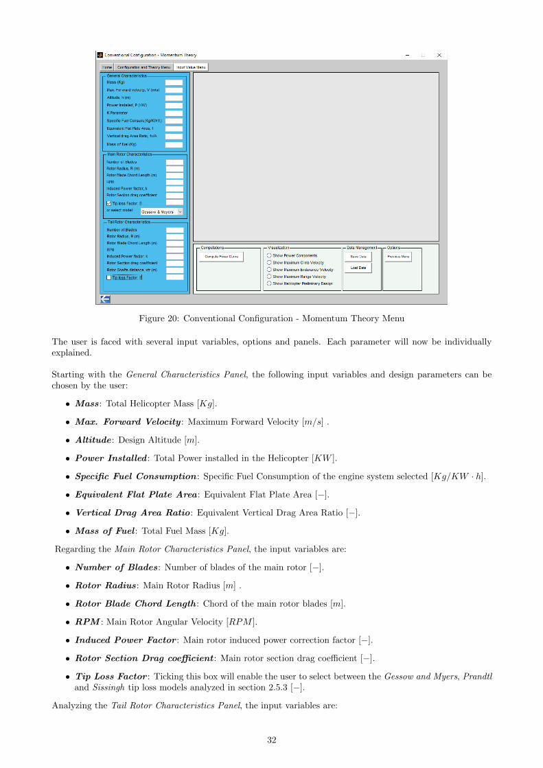
Figure 20: Conventional Configuration - Momentum Theory Menu
The user is faced with several input variables, options and panels. Each parameter will now be individuallyexplained.
Starting with the General Characteristics Panel, the following input variables and design parameters can bechosen by the user:
• Mass: Total Helicopter Mass [Kg].
• Max. Forward Velocity : Maximum Forward Velocity [m/s] .
• Altitude : Design Altitude [m].
• Power Installed : Total Power installed in the Helicopter [KW ].
• Specific Fuel Consumption : Specific Fuel Consumption of the engine system selected [Kg/KW · h].
• Equivalent Flat Plate Area : Equivalent Flat Plate Area [−].
• Vertical Drag Area Ratio: Equivalent Vertical Drag Area Ratio [−].
• Mass of Fuel : Total Fuel Mass [Kg].
Regarding the Main Rotor Characteristics Panel, the input variables are:
• Number of Blades: Number of blades of the main rotor [−].
• Rotor Radius: Main Rotor Radius [m] .
• Rotor Blade Chord Length : Chord of the main rotor blades [m].
• RPM : Main Rotor Angular Velocity [RPM ].
• Induced Power Factor : Main rotor induced power correction factor [−].
• Rotor Section Drag coefficient : Main rotor section drag coefficient [−].
• Tip Loss Factor : Ticking this box will enable the user to select between the Gessow and Myers, Prandtland Sissingh tip loss models analyzed in section 2.5.3 [−].
Analyzing the Tail Rotor Characteristics Panel, the input variables are:
32

• Number of Blades: Number of blades of the tail rotor [−].
• Rotor Radius: Tail Rotor Radius [m] .
• Rotor Blade Chord Length : Chord of the tail rotor blades [m].
• RPM : Tail Rotor Angular Velocity [RPM ].
• Induced Power Factor : Tail rotor induced power correction factor [−].
• Rotor Section Drag coefficient : Tail rotor section drag coefficient [−].
• Rotor Shafts distance : Distance between the main and tail rotor shafts [m].
• Tip Loss Factor : Ticking this box will enable the user to select between the Gessow and Myers, Prandtland Sissingh tip loss models analyzed in section 2.5.3 [−].
If the user does not know the value of a certain parameter for his design, or if that parameter is not relevantfor the design that the user wants to test, leaving the parameter input space blank, will imply that a defaultvalue will be attributed to that parameter. The list of default values is the following:
• Mass: m = 3500 Kg
• Max. Forward Velocity : V∞max= 75 m/s .
• Altitude : h = 1500 m
• Power Installed : Pinst = 2000 KW
• Specific Fuel Consumption : SFC = 0.5640 Kg/KW · h
• Equivalent Flat Plate Area The default value of the equivalent flat plate area will depend on thehelicopter total mass, m, as following [6]:
f =
0.93, for m ≤ 2000.
2.8, for 2000 < m ≤ 7000
3.5, for 7000 < m ≤ 12000
4.65, for 12000 < m ≤ 25000
6 for m > 25000
(181)
• Vertical Drag Area Ratio: fvA = 0.1
• Mass of Fuel : WF = 500 Kg.
Regarding the Main Rotor Characteristics Panel, the default values are:
• Number of Blades: Nb = 4
• Rotor Radius The default value of the main rotor radius, R, will depend on the maximum forwardvelocity, V∞, and on the helicopter total mass, m. Using the empirical formulas developed in [1], thedefault value of R, in meters, will be given by:
R = 4.5667 ·m0.380 · (3.6 · V∞max)−0.515
(182)
• Rotor Blade Chord Length : The default value of the main rotor chord length, c, will depend on thenumber of blades of the main rotor, Nb, and on the helicopter total mass, m. According to the empiricalformulas developed in [1], the default value of c, in meters, will be given by:
c = 0.0108 ·m0.539 ·Nb−0.714 (183)
• RPM : The default value of the main rotor angular velocity, Ω, will depend on main rotor radius, R.According to the empirical formulas developed in [1], the default value of Ω, in RPM, will be given by:
Ω =2673
(2R)0.829 (184)
33

• Induced Power Factor : k = 1.15
• Rotor Section Drag coefficient : Cd0= 0.008
• Tip Loss Factor : The default tip loss model is the Gessow and Myers model, where the tip loss factor,B, is given by:
B = 1− c
2R(185)
and for the Tail Rotor Characteristics Panel :
• Number of Blades: Nbtr = 4
• Rotor Radius The default value of the tail rotor radius, Rtr, will depend on the helicopter total mass,m. Using the empirical formulas developed in [1], the default value of Rtr, in meters, will be given by:
Rtr = 0.0443 ·m0.393 (186)
• Rotor Blade Chord Length : The default value of the tail rotor chord length, ctr, will depend on thenumber of blades of the main rotor, Nbtr , and on the helicopter total mass, m. According to the empiricalformulas developed in [1], the default value of ctr, in meters, will be given by:
ctr = 0.0058 ·m0.506 ·Nbtr−0.72 (187)
• RPM : The default value of the tail rotor angular velocity, Ωtr, will depend on main rotor radius, Rtr.According to the empirical formulas developed in [1], the default value of Ωtr, in RPM, will be given by:
Ωtr =3475
(2Rtr)0.828 (188)
• Induced Power Factor : ktr = 1.15
• Rotor Section Drag coefficient : Cd0tr= 0.008
• Rotor Shafts distance : The default value of the distance between the main and tail rotor shafts, xtr,will depend on main rotor diameter, D. According to the empirical formulas developed in [1], the defaultvalue of xtr, in meters, will be given by:
xtr = 0.5107 ·D1.061; (189)
• Tip Loss Factor : The default tip loss model is the Gessow and Myers model, where the tip loss factor,Btr, is given by:
Btr = 1− ctr2Rtr
(190)
3.2.2 Total Power Requirements Evaluation
After having selected all the design input values, the user should click on the Compute Power Curve buttonlocated on the Computations Panel. The computation of total power requirements as function of the forwardvelocity of the helicopter will now be performed in according with the following MATLAB routine steps:
1. Computation of helicopter weight (W ), rotor disk area (A), design density (ρ) and main rotor solidity (σ)by the following equations:
W = m · g = m · 9.81, (191)
A = πR2, (192)
ρ = ρ0 · e(−0.0296h
304.8 ), (134)
σ =Nbc
πR(193)
34
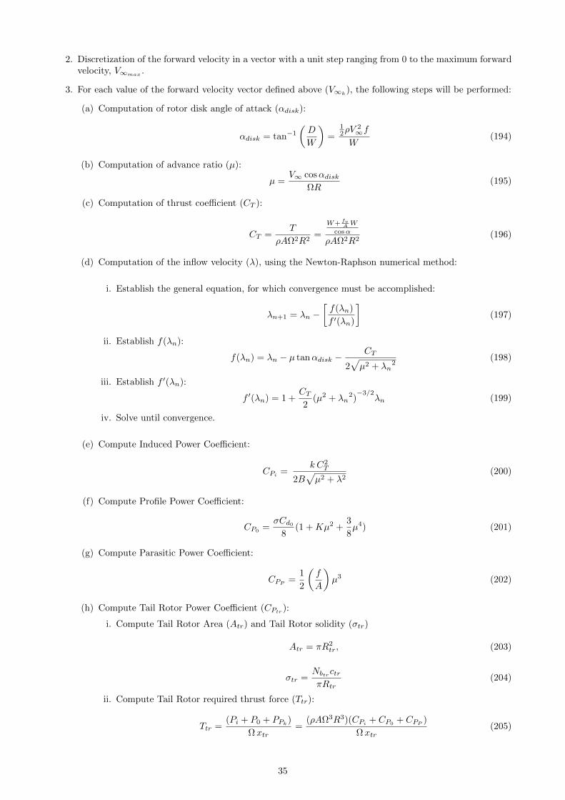
2. Discretization of the forward velocity in a vector with a unit step ranging from 0 to the maximum forwardvelocity, V∞max
.
3. For each value of the forward velocity vector defined above (V∞k), the following steps will be performed:
(a) Computation of rotor disk angle of attack (αdisk):
αdisk = tan−1
(D
W
)=
12ρV
2∞f
W(194)
(b) Computation of advance ratio (µ):
µ =V∞ cosαdisk
ΩR(195)
(c) Computation of thrust coefficient (CT ):
CT =T
ρAΩ2R2=
W+ fvA W
cosα
ρAΩ2R2(196)
(d) Computation of the inflow velocity (λ), using the Newton-Raphson numerical method:
i. Establish the general equation, for which convergence must be accomplished:
λn+1 = λn −[f(λn)
f ′(λn)
](197)
ii. Establish f(λn):
f(λn) = λn − µ tanαdisk −CT
2√µ2 + λn
2(198)
iii. Establish f ′(λn):
f ′(λn) = 1 +CT2
(µ2 + λn2)−3/2
λn (199)
iv. Solve until convergence.
(e) Compute Induced Power Coefficient:
CPi =k C2
T
2B√µ2 + λ2
(200)
(f) Compute Profile Power Coefficient:
CP0=σCd0
8(1 +Kµ2 +
3
8µ4) (201)
(g) Compute Parasitic Power Coefficient:
CPP =1
2
(f
A
)µ3 (202)
(h) Compute Tail Rotor Power Coefficient (CPtr ):
i. Compute Tail Rotor Area (Atr) and Tail Rotor solidity (σtr)
Atr = πR2tr, (203)
σtr =NbtrctrπRtr
(204)
ii. Compute Tail Rotor required thrust force (Ttr):
Ttr =(Pi + P0 + PPk)
Ωxtr=
(ρAΩ3R3)(CPi + CP0+ CPP )
Ωxtr(205)
35

iii. Compute Tail Rotor Thrust Coefficient (CTtr ):
CTtr =Ttr
ρAtrΩ2trR
2tr
, (206)
iv. Computation of the inflow velocity (λtr) using the Newton-Raphson numerical method:
A. Establish the general equation, for which convergence must be accomplished:
λtrn+1 = λtrn −[f(λtrn)
f ′(λtrn)
](207)
B. Establish f(λtrn):
f(λtrn) = λtrn −CTtr
2√µ2 + λtrn
2(208)
C. Establish f ′(λtrn):
f ′(λtrn) = 1 +CTtr
2(µ2 + λtrn
2)−3/2
λtrn (209)
D. Solve until convergence.
v. Solve for Tail Rotor Total Power Coefficient (CPtr ):
CPtr =k C2
Ttr
2Btr√µ2 + λ2
tr
+σtrCd0tr
8(1 +Ktr µ
2) (210)
(i) Compute Total Power (Pk):
Pk = (ρAΩ3R3) · (CPi + CP0+ CPP ) + (ρAtrΩ
3trR
3tr) · CPtr (211)
4. Store the Pk value obtained for each value of V∞k.
The plot of the power requirements curve (Pk) as a function of the forward velocity (V∞k) will now be shown:
Figure 21: Configuration and Theory Selection Menu - Power Curve Results
The user can now select several options in the Visualization Panel. Starting by analyzing the Show PowerComponents button, clicking this option will plot the individual contribution of each power term to the totalpower curve, as following:
36

Figure 22: Configuration and Theory Selection Menu - Show Power Components option
The induced, profile, parasitic and tail rotor power curves are now plotted individually.
Regarding the Show Maximum Climb Velocity, selecting this option will perform the calculation of the maxi-mum climb velocity, based on the climb power available for each forward velocity value, as analyzed in section2.5.5. The climb power available will be given by the difference of the power installed curve and the total powerrequirements curve. Therefore the maximum climb velocity can be computed by:
Vck =Pinst − Pk
W(212)
The plot of the maximum climb velocity curve (Vck) as a function of the forward velocity (V∞k) will now be
shown:
Figure 23: Configuration and Theory Selection Menu - Show Maximum Climb Velocity option
Analyzing the Show Maximum Endurance Velocity button, selecting this option will compute the maximum
37

endurance of the designed helicopter, together with the forward velocity value for which the maximum endurancecan be attainable. Recalling the analysis done in equation (157), the forward velocity for which the maximumendurance can be reached, is given by the velocity that yields the minimum value of the total power requirementscurve. Using the minimum value of the total power requirements curve, the maximum endurance will be givenby:
E ≈WF
[1
P · SFC
]WGTOW−Wf/2
(213)
The maximum endurance value and the power and velocity values for which the maximum endurance is attain-able, will now be computed and identified in the power requirements curve:
Figure 24: Configuration and Theory Selection Menu - Show Maximum Endurance Velocity option
Regarding the Show Maximum Range Velocity button, selecting this option will compute the maximum rangeof the designed helicopter, together with the forward velocity value for which the maximum range can beattainable. Recalling the analysis done in section 2.5.7, the forward velocity for which the maximum range canbe reached, is given by the velocity that yields the minimum value of the ratio between the power required valueand the forward velocity value. Using the velocity and power values associated with the minimum of this ratio,the maximum range will be given by:
Ra ≈WF
[V
P · SFC
]WGTOW−Wf/2
(163)
The maximum range value and the power and velocity values for which the maximum range is attainable, willnow be computed and identified in the power requirements curve:
38

Figure 25: Configuration and Theory Selection Menu - Show Maximum Range Velocity option
3.2.3 Dimensional Design
Analyzing the Show Helicopter Preliminary Design button, selecting this option will open a new panel, withthe preliminary dimensional design of the helicopter. The dimensional design values are the following:
• Helicopter Height (Hh)
• Helicopter Length (Lh)
• Helicopter Length (Wh)
• Helicopter Tip-to-Tip Length (Th)
• Main Rotor Diameter (D)
• Tail Rotor Diameter (Dtr)
where D and Dtr were obtained with the input values given by the user and/or by the default values. Regardingthe values of Hh, Lh, Wh and Th, they will be computed by using the following empirical formulas developedin [1]:
• Helicopter Height (Hh):Hh = 0.642 ·D0.677 (214)
• Helicopter Length (Lh):Lh = 0.824 ·D1.056 (215)
• Helicopter Width (Wh):Wh = 0.436 ·D0.697 (216)
• Helicopter Tip-to-Tip Length (Th):Th = 1.09 ·D1.03 (217)
and the following results panel will be shown:
39

Figure 26: Helicopter Prelininary Design Panel
3.2.4 Tandem and Co-Axial Configurations
The Momentum Theory graphical user interface for tandem and co-axial configurations is very identical to theconventional configuration interface. However, there are slight changes which will be addressed in this section.
Tandem ConfigurationStarting with the tandem configuration and with the main input value menu, one important difference can bedetected. There is no dedicated panel for the tail rotor characteristics, since in this configuration a tail rotoris not required. Also, the Main Rotor Characteristics panel will now be dedicated to the design of the 2 mainrotors. Furthermore, the option to chose the interference power factor (kov) is now available. The default valueof this parameter is given by:
kov = 1.14 [−] (218)
Figure 27: Tandem Configuration - Momentum Theory Menu
Regarding the code structure and implementation, the MATLAB routine for the tandem configuration is similar
40

to the conventional. The slight differences/adaptations to this configuration will now be pointed out:
• Step 3.(c): Since for the tandem configuration, each rotor must produce half the total thrust required,the thrust coefficient will be re-defined as:
CT =T
ρAΩ2R2=
W/2(1+ fvA )
cosα
ρAΩ2R2(219)
• Step 3.(e) and 3.(h): Since for the tandem configuration, there are two main rotors, the total inducedand profile powers, taking in account the considerations made for equations (70) and (72), will be givenby:
CPi = 2kov k C
2T
2B√µ2 + λ2
(220)
and:
CP0 = 2σCd0
8(1 +Kµ2 +
3
8µ4) (221)
for advance ratio values ≤ 0.1. For µ > 0.1, the induced and profile powers will be given by:
CPi =k C2
T
2B√µ2 + λ2
+kov k C
2T
2B√µ2 + λ2
(222)
and:
CP0 = 2σCd0
8(1 +Kµ2 +
3
8µ4) (223)
It should be mentioned that all the remaining parameters, default values and functionalities are the same asthe ones from the conventional configuration interface.
Co-Axial ConfigurationRegarding the co-axial configuration interface, it will be identical to the tandem configuration one. Similarly,there will be the option to directly input the interference power factor (now designated as kint) in the mainmenu. The default value of this parameter is:
kint = 1.16 [−] (224)
Regarding the MATLAB implementation, taking in account the considerations made for equation (63), the totalinduced and profile powers, at steps 3.(e) and 3.(h), will be given by:
CPi = 2kint k C
2T
2B√µ2 + λ2
(225)
and:
CP0= 2
σCd0
8(1 +Kµ2 +
3
8µ4) (226)
It should be mentioned that these equations are identical to the ones applied for the tandem configuration forvalues of the advance ratio (µ) ≤ 0.1, but with the appropriate interference power factor applied for the inducedpower computation.
3.3 Blade Element Theory Model
3.3.1 User Inputs
When compared to the Momentum Theory, the graphical user interface for Blade Element Theory is far morecomplex and complete, providing the user with more functionalities, dedicated menus, input variables and de-sign choices. However, the computational time required to perform the calculations can be several times greaterthen the one required for Momentum Theory computations.
41

Figure 28: Co-Axial Configuration - Momentum Theory Menu
After choosing the Blade Element Theory option on the Configuration and Theory Selection Menu, the followingwindow will be shown:
Figure 29: Conventional Configuration - Blade Element Theory Menu
Some differences can already be seen when compared with the Momentum Theory interface. First in GeneralCharacteristics Panel, the Power Installed value was replaced by the Power Plant dedicated menu. Also there isnow the Fuselage design dedicated menu. In the Main and Tail Rotor Characteristics panel, there is the BladePlanform Selection Menu (which besides including the main rotor characteristics available on the MomentumTheory Interface, will present some more design values) and the Airfoil Selection Menu which will enable theuser to chose the aerodynamics characteristics of the rotors. An important difference is the presence of theB.E.T. Parameters panel. This option will define the integration steps for the radial and azimuthal positions,
42

when integrating numerically the power equations. These parameters are key and will influence the accuracy ofthe results obtained and the computational time required to perform the computations. It should be noted thatthe parameters which are identical to the ones in the Momentum Theory interface, will have the same defaultvalues, meaning and units.Each new feature will now be addressed individually:
• Power Plant MenuWhen selecting this option the following pop-up menu will be shown: This menu will enable the user
Figure 30: Power Plant Menu
to build the powerplant and obtain the total Power Installed value for the designed rotorcraft. Thereis the possibility to select a wide range of engines along with the desired quantity, and obtain real timeinformation about the total power installed, weight and specific fuel consumption of the total enginesystem. By clicking on the Add to Power Plant, a new engine will be added to the powerplant in thequantity selected on the Number of Engines listbox. Clicking on Clear Power Plant option will reset thepowerplant and the total power installed, weight and specific fuel consumption to 0. By selecting theDefault Power Plant option, a powerplant comprised by 2 Pratt&Whitney PT6C − 67C engines with acombined weight of 376 Kg, a specific fuel consumption of 0.306 Kg/KW · h and total power installed of2252 KW, will be selected.
• Fuselage DesignWhen selecting this option, the following pop-up menu will be shown:
Figure 31: Fuselage Design Menu
This menu is dedicated to the estimation of the vertical drag on the fuselage due to the action of the rotorslipstream velocity. To have an accurate estimation of this force, the dimensions of the fuselage core and
43

tail boom must be specified, since the vertical drag coefficient can be different between these two fuselagesections. The following parameters can be chosen by the user:
– Ratio of Boom and Fuselage Length : Ratio between boom length (BL) and fuselage total length(Lh) [−]. The default value is 0.2. The boom length will be found by:
BL = BFL · Lh (227)
where Lh is given by equation (215).
– Ratio of Boom and Fuselage Width : Ratio between boom width (BW ) and fuselage total width(WH) [−]. The default value is 0.2. The boom width will be found by:
BW = BFW ·Wh (228)
where Wh is given by equation (216).
– Fuselage Shape : This option enables the user to choose between a clean, average and bulk fuselagecore shape. The default value is the Clean Configuration. This choice will influence the value ofthe vertical drag coefficient of the fuselage core, as following:
Cdv =
0.4, for Clean Configuration.
0.57, for Average Configuration.
1, for Bulk Configuration.
(229)
Regarding the vertical drag coefficient of the tail boom, due to its clean configuration, it has a fixedvalue of 0.4. After having established the value of the above parameters, the total vertical drag forcecan be computed using equation (180).
Figure 32: Clean, average and bulk fuselage shape examples for the conventional configuration, to be chosen bythe user in the Fuselage Shape panel
• Blade Planform Selection MenuWhen selecting this option the following pop-up menu will be initiated:
Figure 33: Blade Planform Selection Menu - Compute Blade Planform Shape option
44

This menu is dedicated to the rotor design. Here the values of the rotor radius, number of blades and rootchord length can be chosen. The default values will be the same as the ones in the Momentum TheoryInterface. Additionally, there is now the option to chose the chord length at the tip (which will define thetaper ratio), the root-cut-out and the chord distribution model. These will be individually explained:
– Main Rotor Blade Tip Chord Length : Chord length at the blade tip of the main rotor [m].The default value will be given as a function of the blade root chord length as following:
ctip = 0.6 · c0 (230)
– Root-Cut-Out : Ratio between the zero chord blade length (RRCO) and the total blade length ofthe main rotor (R) [%].The default value is:
RCO = 10% (231)
– Chord Distribution Model : Selecting this option will enable the user to select between a linear orhyperbolic chord distribution model. The default model is linear chord distribution model. It shouldbe noted that if the user selects the hyperbolic chord distribution model only the blade tip chordlength can be chosen. These models are used to estimate the chord distribution at each spanwiseposition between the blade root (y = 0) and tip (y = R) and are defined as following:
∗ Linear chord distribution model:
c(y) =ctip − cR
· y (232)
∗ Hyperbolic chord distribution model:
c(y) =
0, for y ≤ 0.2R.ctipRy , for y > 0.2R.
(233)
After having selected the desired input values, clicking on the Compute Blade Planform Shape option willcompute the chord distribution of the main rotor and plot the blade planform shape, as represented infigure (34). The user has also the possibility to have a visual representation/animation of the main rotorby clicking on the option Visualize Main Rotor.
Figure 34: Blade Planform Selection Menu - Visualize Main Rotor option
• Airfoil Selection MenuWhen selecting this option the following pop-up menu will be shown:
45

Figure 35: Airfoil Selection Menu
This menu is mainly focused on the aerodynamic design of the blades. The user has the option to dividethe blade in 3 different sections named root, middle and tip sections. For each section, the user will havethe possibility to select the airfoil shape, the section length and the twist at the root and end of eachsection. This menu will also integrate a compressbility and reverse flow preliminary analysis, where theuser can start to test the aerodynamic behavior/characteristics of the designed rotor. Starting with RootSection Panel, each parameter will now be addressed individually:
– Airfoil : Selection of root section airfoil shape [−]. The default airfoil choice is the NACA 0009.The other available choices for the airfoil section shape are:
Figure 36: Airfoil section shape options
– Section length : Length of root section given in percentage of the rotor blade radius [%]. Thedefault values is:
RSL = 30% (234)
– Blade Twist at section root : Twist angle at the beginning of root section []. The default valuesis:
θrootroot = 10 (235)
– Blade Twist at section end : Twist angle at the end of root section []. The default values is:
θrootend = 10 (236)
For the Middle Section Panel, the input values are:
– Airfoil : Selection of middle section airfoil shape [−]. The default airfoil choice is the NACA 0009.
– Section length : Length of middle section given in percentage of the rotor blade radius [%]. Thedefault values is:
MSL = 30% (237)
46

– Blade Twist at section end : Twist angle at the end of middle section []. The default values is:
θmiddleend = 10 (238)
In this section there is no input value option for the Blade Twist at section root. This happens sincethe Blade Twist at section end of the Root Section coincides with the Blade Twist at section root ofthe Middle Section.
and for the Tip Section Panel :
– Airfoil : Selection of tip section airfoil shape [−]. The default airfoil choice is the NACA 0009.
– Section length : Length of tip section given in percentage of the rotor blade radius [%]. The defaultvalues is:
TSL = 30% (239)
– Blade Twist at section end : Twist angle at the end of tip section []. The default values is:
θtipend = 10 (240)
In this section there is no input value option for the Blade Twist at section root. This happens sincethe Blade Twist at section end of the Middle Section coincides with the Blade Twist at section rootof the Tip Section.
It should be mentioned that the twist distribution along the blade span will be computed by a linearinterpolation between the twist angle values at each section beginning and end points.
Note for the user: The user must make sure that the sum of the 3 blade sections length with theroot-cut-out length must be equal to total blade length. The following equation must always be verified,otherwise an error message will be shown:
RSL+MSL+ TSL+RCO = 100% (241)
After having established the desired input values, the user can now select the 2D Aerodynamic character-istics option on the Computations panel. Clicking this option will compute the polar curves of the chosenairfoils for each blade section. Besides plotting the airfoil shape selected for each blade section, this optionwill give a qualitative analysis of the lift and drag coefficient characteristics as a function of the angle ofthe attack.
Figure 37: Compute 2D Aerodynamics characteristics option
47
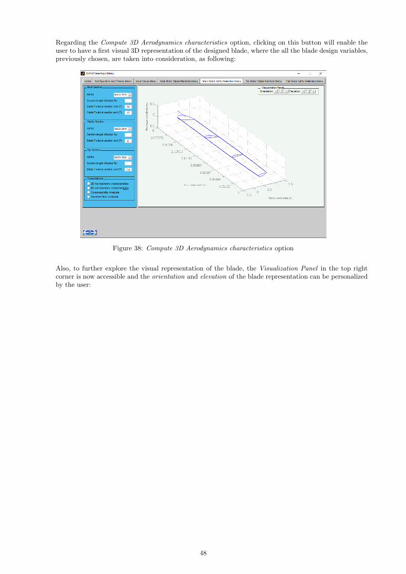
Regarding the Compute 3D Aerodynamics characteristics option, clicking on this button will enable theuser to have a first visual 3D representation of the designed blade, where the all the blade design variables,previously chosen, are taken into consideration, as following:
Figure 38: Compute 3D Aerodynamics characteristics option
Also, to further explore the visual representation of the blade, the Visualization Panel in the top rightcorner is now accessible and the orientation and elevation of the blade representation can be personalizedby the user:
48

Figure 39: Compute 3D Aerodynamics characteristics option - Visualization Panel
Moving forward to the Compressibility analysis option, selecting this button, will open a window dedicatedto the prediction and analysis of compressibility issues. However, the user must first specify the forwardvelocity design point for which the estimation/prediction of the compressibility issues is desired. Theforward velocity design point should be given in percentage of the maximum forward velocity of thedesigned rotorcraft and its value is introduced in the following pop-up box, that will automatically appear:
Figure 40: Compressibility Analysis option - Design point selection
The default value for the forward velocity design point is 70% of the maximum forward velocity value(V∞max
), chosen in the Blade Element Theory Menu. After pressing the OK option, the compressibilityanalysis will be performed and the following results window will appear:
49

Figure 41: Compressibility Analysis option - Results window
All the parameters, results obtained and different functionalities, will now be individually explained:
– Red Area : This region represents the area in which there are compressibility issues, i.e. the rotorregion where the local mach number exceeds the tip airfoil drag divergence mach number, Mdd, and isfound by solving equation (166). Note that the position of the azimuth angles ψ1 and ψ2 is identifiedin the plot of Figure 41, together with the value of advance ratio correspondent to the chosen designpoint.
– Information Panel : This panel includes information about the values of the following parameters:
∗ Current ψ1: Azimuth angle that defines the onset/start of the compressbility affected region[]. Its value is given by equation (167).
∗ Current ψ2: Azimuth angle that defines the end of the compressbility affected region []. Itsvalue is given by ψ2 = 180 − ψ1.
∗ Blade Fraction in Comp. Flow : Fraction of the blade length that is affected by compress-ibility issues [-]. Its value is computed for ψ = 90 and is obtained by solving equation (168).
∗ Current Design Point : Value of the design point for which the compressbility analysis isbeing performed/plotted, given in percentage of the maximum forward velocity [%].
∗ Current Forward Velocity : Value of the forward velocity at the current design point [m/s].
It should be mentioned that the vertical slider located next to this parameter, will enable theuser to increase/decrease the forward velocity for which the compressibility analysis is being per-formed. This functionality allows the user to study quickly, if an increase/decrease of the forwardvelocity relatively to the design point value can have a notorious impact in the compressibilityaffected area. When clicking on the vertical slider, the computation of the compressibility region,azimuthal angles ψ1 and ψ2, Blade Fraction in Compressible Flow, Forward Velocity and DesignPoint, will be redone based on the new value of Forward Velocity. The new values obtainedfor these values will be shown in the Information Panel, together with an updated plot of thecompressibility affected region, the location of ψ1 and ψ2 and the new value of the advance ratioµ. This is depicted in the following figures, where after clicking on the vertical slider top arrow,the increase in the rotorcraft forward velocity, will manisfest as an increase in the compressbilityaffected area:
50

Figure 42: Compressibility Analysis option - Resultswindow for V∞ = 96.6m/s
Figure 43: Compressibility Analysis option - Resultswindow for V∞ = 120.75m/s
Figure 44: Compressibility Analysis option - Results window for V∞ = 160m/s
– Compresibility Panel : This panel is related to the influence of the blade tip shape on thecompressbility issues and will enable the user to modify the blade tip shape in order to reduce thecompressibility effects. This will be adressed through the following parameters:
∗ Design Point for tip shape : Forward velocity value, given in percentange of the maximumforward velocity, for which the tip shade modification sweep angle (Λ) should be computed, inorder to completely eliminate the compressibility issues and compressibility affected area.
∗ Implement tip shape modification : Clicking this option will compute the tip shade modifi-cation sweep angle (Λ) required to eliminate the compressibility issues, based on equation (173)and using the value of the forward velocity design point chosen by the user (figure 40). Thedefault value is zero, i.e. if the user does not click this option, no sweep back angle will beimplemented. After selecting this option the sweep back angle value will be incorporated in themain rotor design and equations, and the updated tip shape will be plotted:
51

Figure 45: Implement tip shape modifications option
Regarding the Reverse Flow analysis, when selecting this option, the following window will appear:
Figure 46: Reverse flow analysis option
It should be mentioned that the design point used to compute the plot represented in Figure 46 will be thesame as the one chosen by the user after selecting the Compressbility Analysis option. All the parameters,results obtained and different functionalities, will now be adressed individually:
– Red Area : This region represents the area in which there is reverse flow, i.e. the rotor region wherethe blade sections operate with the trailing edge into the relative wind, and is found by solvingequation (174). Note that the the value of advance ratio correspondent to the chosen design point isidentified in the plot of figure 46.
52

– Information Panel : This panel includes information about the values of the following parameters:
∗ Blade Fraction in Comp. Flow : Fraction of the blade length that is inside the reverse flowregion [-]. Its value is found by solving equation (174).
∗ Current Design Point : Value of the design point for which the reverse flow analysis is beingperformed/plotted, given in percentage of the maximum forward velocity [%].
∗ Current Forward Velocity : Value of the forward velocity at the current design point [m/s].
It should be mentioned that the vertical slider located next to this parameter, similarly to theone in Compressibility analysis window will enable the user to increase/decrease the forwardvelocity for which the reverse flow analysis is being performed. This functionality allows the userto study quickly, if an increase/decrease of the forward velocity relatively to the design pointvalue can have a notorious impact in the reverse flow region. When clicking on the vertical slider,the computation of the reverse flow region and Blade Fraction in Reverse Flow, will be redonebased on the new value of Forward Velocity. This is depicted in the following figures, whereafter clicking on the vertical slider top arrow, the increase in the rotorcraft forward velocity, willmanisfest as an increase in the reverse flow region:
Figure 47: Reverse Flow Analysis option - Results win-dow for V∞ = 96.6m/s
Figure 48: Reverse Flow Analysis option - Results win-dow for V∞ = 120.75m/s
Figure 49: Reverse Flow Analysis option - Results window for V∞ = 161m/s
• Blade Planform Selection Menu - Tail Rotor : The tail rotor Blade Planform Selection Menu panelwill be identical to the main rotor Blade Planform Selection Menu panel analyzed above, with the sameoptions and functionalities but with the input values adapted for the tail rotor. Hence, to avoid repetition,no individual explanation and guided tutorial will be done to this panel.
• Airfoil Selection Menu - Tail Rotor : The tail rotor Airfoil Selection Menu panel will be identicalto the main rotor Airfoil Selection Menu panel analyzed above, with the same options and functionalities
53

(excluding the compressibility and reverse flow analysis), but with the input values adapted for the tailrotor. Hence, to avoid repetition, no individual explanation and guided tutorial will be done to this panel.
• B.E.T. ParametersIn this panel the the azimuthal and radial discretization steps, for the numerical integration of the totalpower equation, can be selected:
– Integration step of r: Integration step of radial position, given in number of discretization seg-ments. The default value is:
∆r = 10 (242)
The discretization vector the of radial position, r, has (∆r + 1) nodes, and will be discretized asfollowing:
r = [01
∆r
2
∆r
3
∆r... 1] = [r1 ... r∆r+1] (243)
– Integration step of ψ: Integration step of azimuthal position, given in number of discretizationsegments. The default value is:
∆ψ = 10 (244)
The discretization vector the of azimuthal position, ψ, has (∆ψ + 1) nodes, and will be discretizedas following:
ψ = [02π
∆ψ
4π
∆ψ
6π
∆ψ... 2π] = [ψ1 ... ψ∆ψ+1] (245)
3.3.2 Total Power Requirements Evaluation
After having selected all the design input values, the user should click on the Compute Power Curve buttonlocated on the Computations Panel. The computation of total power requirements as function of the forwardvelocity of the helicopter will now be performed in according with the following MATLAB routine steps:
1. Computation of helicopter weight (W ) and rotor disk area (A), by the following equations:
W = m · g = m · 9.81, (191)
A = πR2 (192)
2. Computation of density (ρ), sound speed (a) and dynamic viscosity (µ) at the design altitude:
ρ = ρ0 · e(−0.0296h
304.8 ), (134)
The values of sound speed (a) and dynamic viscosity (µd) will be interpolated from tabled values given asa function of altitude.
3. Creation of main rotor radial and azimuthal position distribution vectors, r and ψ:
r = [01
∆r
2
∆r
3
∆r... 1] (246)
and:
ψ = [02π
∆ψ
4π
∆ψ
6π
∆ψ... 2π] (247)
4. Creation of main rotor chord distribution vector. This line vector will have a size of ∆r + 1 and willincorporate the information about the root-cut-out, main rotor chord distribution model, main rotor rootchord and main rotor tip chord. To exemplify, if the user selects a radial integration step of 5, a root-cut-out value of 0%, and a linear chord distribution model, the main rotor chord distribution vector will bebuilt as:
c (r) = [c c2 c3 c4 c5 ctip]
where the values of c2, c3, c4 and c5 are obtained trough linear interpolation.
54

5. Creation of main rotor twist angle distribution vector. This line vector will have a size of ∆r + 1 and willincorporate the information about the length of each blade section, twist angle at the beggining and endof each blade section and main rotor root-cut-out. To exemplify, if the user selects a radial integrationstep of 10, a root-cut-out value of 0%, a root blade section length of 40%, a middle blade section lengthof 30%, and a tip blade section length of 30%, the main rotor twist angle distribution vector will be builtas:
θ(r) = [θrootroot θ2 θ3 θ4 θrootend θ6 θ7 θmiddleend θ9 θ10 θtipend]
where the values between θrootroot and θrootend , between θrootend and θmiddleend and between θmiddleend and θtipend areobtained trough linear interpolation.
6. Creation of main rotor solidity distribution vector. This line vector will have a size of ∆r + 1 and will begiven by:
σ(r) =Nb c(r)
πR=NbπR
[c c2 c3 c4 c5 ctip] (248)
7. Discretization of the forward velocity in a vector with a 5 m/s step ranging from 0 to the maximumforward velocity, V∞max
.
8. For each value of the forward velocity vector defined above (V∞k), the following steps will be performed:
(a) Computation of rotor disk angle of attack (αdisk):
αdisk = tan−1
(D
W
)=
12ρV
2∞f
W(194)
(b) Computation of advance ratio (µ):
µ =V∞ cosαdisk
ΩR(195)
(c) Computation of thrust coefficient (CT ):
CT =T
ρAΩ2R2=
Wcosαdisk
ρAΩ2R2(249)
(d) Computation of the induced velocity ratio [λi(r, ψ, µ)], using the Newton-Raphson numerical method,for each blade radial and azimutal position, i.e for each value comprising r and ψ:
i. Establish the general equation, for which convergence must be accomplished:
λin+1= λin −
[f(λin)
f ′(λin)
](250)
ii. Establish f(λin):
f(λin) = λin −CT
2√µ2 + λin
2(1 + kxr cos ψ) (251)
where kx is given by:
kx = tan
tan−1(µxλin
)2
(252)
iii. Establish f ′(λin). This equation won’t be written in this section due to its lenghty expression.
iv. Solve until convergence.
Code Note : The vertical drag effects will be included at this step. Having computed the inducedvelocity distribution for each value of r and ψ, and knowing the fuselage width, length and corre-sponding Cdv value at the positions located under the rotor disk it is possible to compute the increasein weight, and therefore, in thrust required, caused by the vertical drag. Assuming that the valueof λi for a given r at ψ = 0 can be considered constant along a strip of width (w) and length (dl)
55
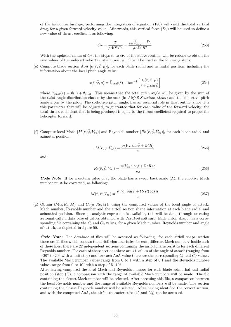
of the helicopter fuselage, performing the integration of equation (180) will yield the total verticaldrag, for a given forward velocity value. Afterwards, this vertical force (Dv) will be used to define anew value of thrust coefficient as following:
CT =T
ρAΩ2R2=
Wcosαdisk
+Dv
ρAΩ2R2(253)
With the updated values of CT , the steps i. to iv. of the above routine, will be redone to obtain thenew values of the induced velocity distribution, which will be used in the following steps.
(e) Compute blade section AoA [α(r, ψ, µ)], for each blade radial and azimutal position, including theinformation about the local pitch angle value:
α(r, ψ, µ) = θtotal(r)− tan−1
[λi(r, ψ, µ)
r + µ sin ψ
](254)
where θtotal(r) = θ(r) + θpilot. This means that the total pitch angle will be given by the sum ofthe twist angle distribution chosen by the user (in Airfoil Selection Menu) and the collective pitchangle given by the pilot. The collective pitch angle, has an essential role in this routine, since it isthis parameter that will be adjusted, to guarantee that for each value of the forward velocity, thetotal thrust coefficient that is being produced is equal to the thrust coefficient required to propel thehelicopter forward.
(f) Compute local Mach [M(r, ψ, V∞)] and Reynolds number [Re (r, ψ, V∞)], for each blade radial andazimutal position:
M(r, ψ, V∞) =ρ (V∞ sin ψ + ΩrR)
a(255)
and:
Re(r, ψ, V∞) =ρ (V∞ sin ψ + ΩrR) c
µd(256)
Code Note : If for a certain value of r, the blade has a sweep back angle (Λ), the effective Machnumber must be corrected, as following:
M(r, ψ, V∞) =ρ (V∞ sin ψ + ΩrR) cos Λ
a(257)
(g) Obtain Cl(α,Re,M) and Cd(α,Re,M), using the computed values of the local angle of attack,Mach number, Reynolds number and the airfoil section shape information at each blade radial andazimuthal position. Since no analytic expression is available, this will be done through accessingautomatically a data base of values obtained with JavaFoil software. Each airfoil shape has a corre-sponding file containing the Cl and Cd values, for a given Mach number, Reynolds number and angleof attack, as depicted in figure 50.
Code Note : The database of files will be accessed as following: for each airfoil shape sectionthere are 11 files which contain the airfoil characteristics for each different Mach number. Inside eachof these files, there are 22 independent sections containing the airfoil characteristics for each differentReynolds number. For each of these sections there are 41 values of the angle of attack (ranging from−20 to 20 with a unit step) and for each AoA value there are the corresponding Cl and Cd values.The available Mach number values range from 0 to 1 with a step of 0.1 and the Reynolds numbervalues range from 0 to 107 with a step of 5 · 105.After having computed the local Mach and Reynolds number for each blade azimuthal and radialposition (step (f)), a comparison with the range of available Mach numbers will be made. The filecontaining the closest Mach number will be selected. After accessing this file, a comparison betweenthe local Reynolds number and the range of available Reynolds numbers will be made. The sectioncontaining the closest Reynolds number will be selected. After having identified the correct section,and with the computed AoA, the airfoil characteristics (Cl and Cd) can be accessed.
56
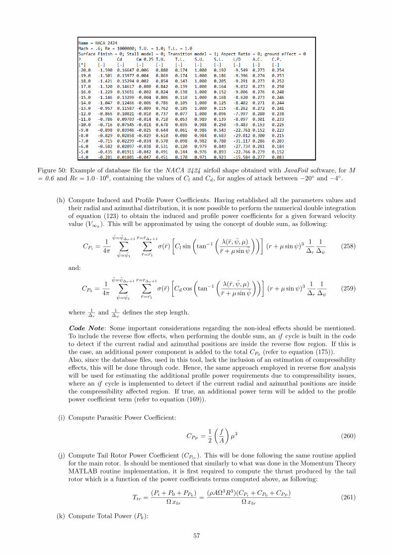
Figure 50: Example of database file for the NACA 2424 airfoil shape obtained with JavaFoil software, for M= 0.6 and Re = 1.0 · 106, containing the values of Cl and Cd, for angles of attack between −20 and −4.
(h) Compute Induced and Profile Power Coefficients. Having established all the parameters values andtheir radial and azimuthal distribution, it is now possible to perform the numerical double integrationof equation (123) to obtain the induced and profile power coefficients for a given forward velocityvalue (V∞k
). This will be approximated by using the concept of double sum, as following:
CPi =1
4π
ψ=ψ∆r+1∑ψ=ψ1
r=r∆r+1∑r=r1
σ(r)
[Cl sin
(tan−1
(λ(r, ψ, µ)
r + µ sin ψ
))](r + µ sinψ)3 1
∆r
1
∆ψ(258)
and:
CP0 =1
4π
ψ=ψ∆r+1∑ψ=ψ1
r=r∆r+1∑r=r1
σ(r)
[Cd cos
(tan−1
(λ(r, ψ, µ)
r + µ sin ψ
))](r + µ sinψ)3 1
∆r
1
∆ψ(259)
where 1∆r
and 1∆ψ
defines the step length.
Code Note : Some important considerations regarding the non-ideal effects should be mentioned.To include the reverse flow effects, when performing the double sum, an if cycle is built in the codeto detect if the current radial and azimuthal positions are inside the reverse flow region. If this isthe case, an additional power component is added to the total CP0 (refer to equation (175)).Also, since the database files, used in this tool, lack the inclusion of an estimation of compressibilityeffects, this will be done through code. Hence, the same approach employed in reverse flow analysiswill be used for estimating the additional profile power requirements due to compressibility issues,where an if cycle is implemented to detect if the current radial and azimuthal positions are insidethe compressibility affected region. If true, an additional power term will be added to the profilepower coefficient term (refer to equation (169)).
(i) Compute Parasitic Power Coefficient:
CPP =1
2
(f
A
)µ3 (260)
(j) Compute Tail Rotor Power Coefficient (CPtr ). This will be done following the same routine appliedfor the main rotor. Is should be mentioned that similarly to what was done in the Momentum TheoryMATLAB routine implementation, it is first required to compute the thrust produced by the tailrotor which is a function of the power coefficients terms computed above, as following:
Ttr =(Pi + P0 + PPk)
Ωxtr=
(ρAΩ3R3)(CPi + CP0+ CPP )
Ωxtr(261)
(k) Compute Total Power (Pk):
57

Pk = (ρAΩ3R3) · (CPi + CP0+ CPP ) + (ρAtrΩ
3trR
3tr) · CPtr (262)
9. Store the Pk value obtained for each value of V∞k.
The plot of the power requirements curve (Pk) as a function of the forward velocity (V∞k) will be shown:
Figure 51: Configuration and Theory Selection Menu - Show Power Components option
Regarding the Show Power Components, Show Maximum Climb Velocity, Show Maximum Endurance Velocity,Show Maximum Range Velocity and Show Helicopter Preliminary Design options, their computation, layoutand design will be identical to the ones defined Momentum Thoery Interface. Hence to avoid repetition, theseoptions will not be shown in the context of Blade Element Theory. An additional feature that is only availablefor the Blade Element Theory user interface, is the Show Pilot Collective Pitch option. When selecting thisoption the following animation will be initiated:
Figure 52: Show Pilot Collective Pitch option Figure 53: Show Pilot Collective Pitch option
This animation shows the collective pitch angle (θpilot) value for each value of the forward velocity. This is theminimum value that the pilot must input to guarantee that the total thrust coefficient that is being producedis equal to the thrust coefficient required to propel the helicopter forward.
58
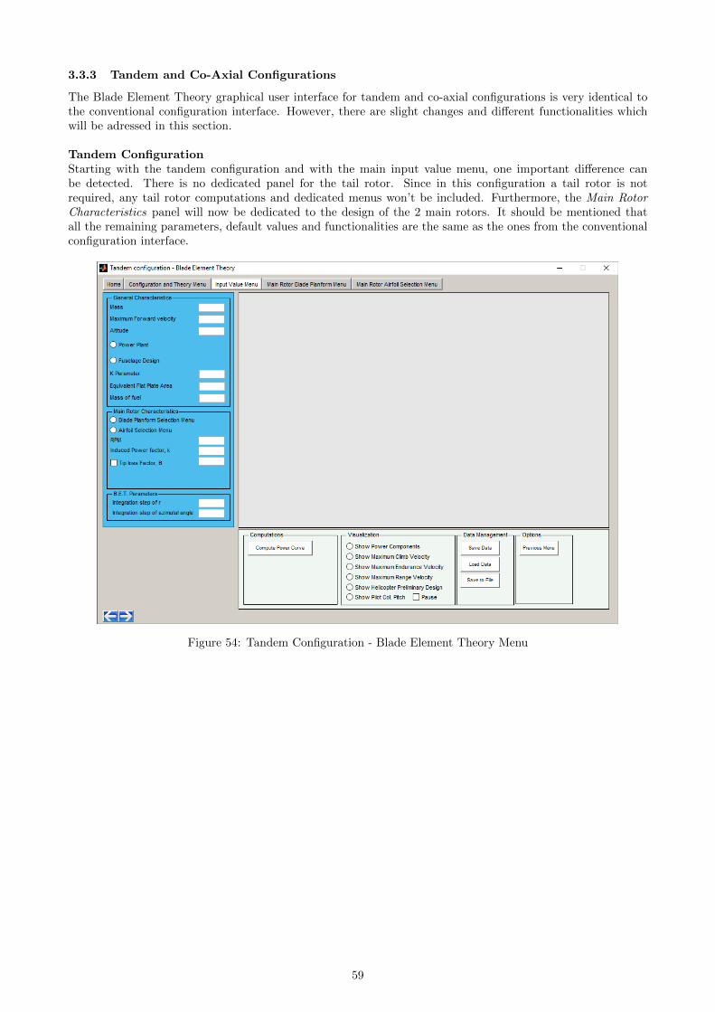
3.3.3 Tandem and Co-Axial Configurations
The Blade Element Theory graphical user interface for tandem and co-axial configurations is very identical tothe conventional configuration interface. However, there are slight changes and different functionalities whichwill be adressed in this section.
Tandem ConfigurationStarting with the tandem configuration and with the main input value menu, one important difference canbe detected. There is no dedicated panel for the tail rotor. Since in this configuration a tail rotor is notrequired, any tail rotor computations and dedicated menus won’t be included. Furthermore, the Main RotorCharacteristics panel will now be dedicated to the design of the 2 main rotors. It should be mentioned thatall the remaining parameters, default values and functionalities are the same as the ones from the conventionalconfiguration interface.
Figure 54: Tandem Configuration - Blade Element Theory Menu
59

Regarding the Fuselage Design dedicated menu, some modifications were implemented:
Figure 55: Tandem Configuration - Fuselage Design Menu
As shown in the figure above, the user has the possibility to choose the ratio between the dimensions of thefuselage core (the wider and shorter part) and the fuselage, as following:
• Ratio of core and fuselage length : Ratio between fuselage core length (FCL) and fuselage totallength (Lh) [−]. The default value is 0.8. The fuselage core length (CL) will be found by:
CL = FCL · Lh (263)
where Lh is given by equation (215).
• Ratio of fuselage and core width : Ratio between fuselage width (FW ) and fuselage core width (Wh)[−]. The default value is 0.8. The fuselage width will be found by:
FW = CFW ·Wh (264)
Moving forward to the Blade Planform Selection Menu, a new option designated as Rotor Placement Panel isnow available:
Figure 56: Tandem Configuration - Blade Planform Selection Menu
60

Figure 57: Tandem Configuration - Rotor Placement Panel option
This new menu will be dedicated to the choice of the relative position between the 2 main rotors. When selectingthis option the following window will be shown:All the parameters, results obtained and different functionalities of this window, will be adressed individually:
• Horizontal Placement slider : This is the key parameter in this dedicated menu and will influence allthe values of the parameters obtained in this window. With the slider, the user can increase/decrease thedistance between the main rotors shaft by clicking on the right/left arrows, and for the chosen distanceobtain real time information about the interference power factor and about the overlapping area of thechosen design. The default value of this slider will yield a rotorshaft distance of 5m.
• Red Area : This region represents the area in which, for a chosen distance between the two rotors, thereis an overlap of the two main rotors.
• Information Panel : This panel includes information about the values of the following parameters:
– kov: Interference power factor [-]. Its value is given by equation (68).
– Ratio of Overlap and disk area : Represents the ratio between the overlapping area (red area)and the main rotor disk area. Its value is given by equation (64).
– Distance between rotorshafts: Distance between the 2 main rotor shafts. Its value will be givenby moving the Horizontal Placement slider to the desired position.
It should be mentioned that if the user decreases the rotorshaft distance below the rotor radius value (R), awarning message stating that the user should increase the rotorshaft distance, will be displayed, since for thesevalues the blades of the main rotors will be overlapping with the rotorshafts which is an impossible situation.
61

Figure 58: Rotor placement plot for a distance betweenrotorshafts of 9.42m (1.7R)
Figure 59: Rotor placement plot for a distance betweenrotorshafts of 6.73m (1.3R)
Figure 60: Rotor placement plot for a distance between rotorshafts of 4.5m (0.9R) with display of a warningmessage
Regarding the code structure and implementation, the MATLAB routine for the tandem configuration is similarto the conventional. The slight differences/adaptations to this configuration will now be pointed out:
• Step 8.(c): Since for the tandem configuration, each rotor must produce half the total thrust required,the thrust coefficient will be re-defined as:
CT =T/2
ρAΩ2R2=
W/2cosαdisk
ρAΩ2R2(265)
• Step 8.(h): Since for the tandem configuration, there are two main rotors contributing to the totalinduced and profile powers, and taking in account the considerations made for equations (131) and (133),the numerical integration will be based on the following equations:
CPi =1
4π
ψ=ψ∆r+1∑ψ=ψ1
r=r∆r+1∑r=r1
σ(r)
[2kov Cl sin
(tan−1
(λ(r, ψ, µ)
r + µ sin ψ
))](r + µ sinψ)3 1
∆r
1
∆ψ(266)
and:
CP0=
1
4π
ψ=ψ∆r+1∑ψ=ψ1
r=r∆r+1∑r=r1
σ(r)
[2Cd cos
(tan−1
(λ(r, ψ, µ)
r + µ sin ψ
))](r + µ sinψ)3 1
∆r
1
∆ψ(267)
for advance ratio values ≤ 0.1. For µ > 0.1, the numerical integration will be performed on:
CPi =1
4π
ψ=ψ∆r+1∑ψ=ψ1
r=r∆r+1∑r=r1
σ(r)
[(1 + kov)Cl sin
(tan−1
(λ(r, ψ, µ)
r + µ sin ψ
))](r + µ sinψ)3 1
∆r
1
∆ψ(268)
and:
CP0=
1
4π
ψ=ψ∆r+1∑ψ=ψ1
r=r∆r+1∑r=r1
σ(r)
[2Cd cos
(tan−1
(λ(r, ψ, µ)
r + µ sin ψ
))](r + µ sinψ)3 1
∆r
1
∆ψ(269)
62
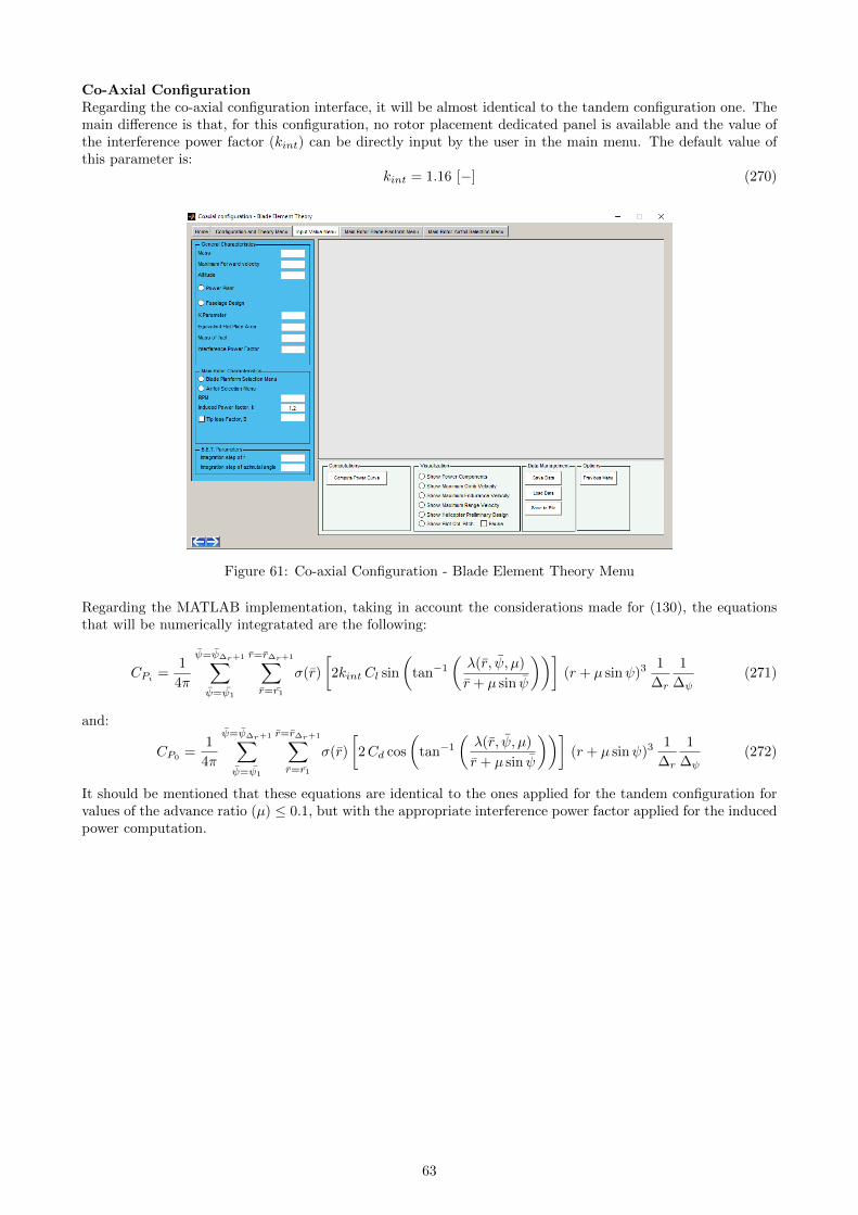
Co-Axial ConfigurationRegarding the co-axial configuration interface, it will be almost identical to the tandem configuration one. Themain difference is that, for this configuration, no rotor placement dedicated panel is available and the value ofthe interference power factor (kint) can be directly input by the user in the main menu. The default value ofthis parameter is:
kint = 1.16 [−] (270)
Figure 61: Co-axial Configuration - Blade Element Theory Menu
Regarding the MATLAB implementation, taking in account the considerations made for (130), the equationsthat will be numerically integratated are the following:
CPi =1
4π
ψ=ψ∆r+1∑ψ=ψ1
r=r∆r+1∑r=r1
σ(r)
[2kint Cl sin
(tan−1
(λ(r, ψ, µ)
r + µ sin ψ
))](r + µ sinψ)3 1
∆r
1
∆ψ(271)
and:
CP0=
1
4π
ψ=ψ∆r+1∑ψ=ψ1
r=r∆r+1∑r=r1
σ(r)
[2Cd cos
(tan−1
(λ(r, ψ, µ)
r + µ sin ψ
))](r + µ sinψ)3 1
∆r
1
∆ψ(272)
It should be mentioned that these equations are identical to the ones applied for the tandem configuration forvalues of the advance ratio (µ) ≤ 0.1, but with the appropriate interference power factor applied for the inducedpower computation.
63

4 Results
The main goal of this section is to evaluate if the tool developed is producing accurate results, for the threedifferent rotorcraft configurations and two theories implemented. The most effective way to accomplish thisevaluation is to select a known configuration of an already developed rotorcraft, input all its available designparameters in the tool, compute the power curve, maximum endurance and maximum range characteristicsand compare the results obtained with the specifications of the manufacturer. The chosen helicopters, for eachconfiguration, to launch the simulation, are the following:
• Conventional Configuration: Bell 429
• Tandem Configuration: Boeing CH-47 Chinook
• Co-axial Configuration: Kamov Ka-27
For each model selected, the results obtained with Momentum and Blade Element Theory will now be analyzed.
4.1 Influence of Radial and Azimuthal Discretization Step Values
Before running the power curve computations for the Blade Element Theory interface, a study about the influ-ence of the radial and azimuthal steps on the results obtained, must be performed, to guarantee that convergedresults are being produced. This study will be done by fixing a value of the forward velocity, and analyze theresults obtained when the number of discritization segments start to increase. If, when increasing the numberof discretization segments, the results show a tendency to converge to a given value, than the value of thediscretization steps which will be chosen for the estimating the power curves for the Blade Element Theoryinterface (in the following sections) will be based on the lowest value that yields results inside the convergencezone. With this approach, accurate results will be produced and, at the same time, the computational time willbe minimized.
Starting with the analysis, the value chosen for forward velocity is 60 m/s, and the initial value of the numberof discretization segments is 5, both for the radial and azimuthal values. Analyzing first, the influence of thenumber of radial discretization segments, this value will be continuously increased by 5 units (while fixing thenumber of the azimuthal discretization segments at 10). The results obtained are shown in figure 62:
Figure 62: Influence of the number of radial discretization segments at V∞ = 60 m/s
It is visible that around the value of 60 radial discretization segments, the results obtained start to converge.This will be the chosen value for the number of radial discretization segments.
Analyzing now the influence of the number of azimuthal discretization segments, a similar approach will beemployed. Hence, starting at the value of 5 and continuously increase the number of azimuthal discretizationsegments (while fixing the number of the radial discretization segments at 10), will yield the results show in
64

figure (63):
Figure 63: Influence of the number of azimuthal discretization segments at V∞ = 60 m/s
As before, it is clear that around the value of 70 azimuthal discretization segments, the results obtained startto converge.
However, an analysis of the computational time required still needs to be performed. If the computationaltime required to perform the calculations using the value of 60, for the number of radial discretization segments,and 70, for the azimuthal discretization segments, is very high, possibly the gain in accuracy does not compen-sate the increase in computational time. This choice will be done by the user, but a computational time analysiswill be done, to aid in this choice. Starting with the number of radial and azimuthal discretization segmentsequal to 5, and increasing consecutively these values by 10, a plot of the increase in computational time (givenin number of times that the time obtained is greater than the time obtained with the first values of radial andazimuthal discretization segments) will be plotted, together with the relative error obtained (using as referencethe power value obtained when using 80 radial and azimuthal discretization steps), as following:
Figure 64: Influence of the number of discretization steps on the computational time required (normalized withthe time obtained for the first values of azimuthal and radial steps, i.e. the time obtained for a certain value ofthe number of steps is given in the number of times that the time obtained is greater than the time obtainedwith 5 radial and azimuthal discretization segments) and on the relative error obtained at V∞ = 60 m/s
65

Analyzing Figure 64, it is possible to conclude that when choosing 70 azimuthal and radial discretizations steps,instead of 30, although the relative error decreases 2.9 %, the computational time is 80 times higher. This showsthat, sometimes, increasing the number of discretization steps, even if the relative error decreases, the increasein computational time does not compensate the higher accuracy. Due to the reasons stated above, the numberof azimuthal and radial discretizations steps, that will be chosen for the simulations that will be performed inthe following sections, will be 30, in order to obtain a faster and more sustainable analysis (since the user hasno interest in a computational time of several hours), without loosing relevant accuracy.
4.2 Results obtained for Conventional Configuration
Regarding the model Bell 429, the design parameters whose value was found in the available literature, are thefollowing:
• Maximum Take Off mass (m): 3402 Kg
• Maximum Forward Velocity (V∞max): 287 km/h = 79.7 m/s
• Power Plant (Pinst): 820 KW (2x Pratt & Whitney Canada PW207D1)
• Specific Fuel Consumption (SFC): 0.329 Kg/KW · h
• Fuel Mass (WF ): 630 Kg (821 L deposit and fuel density of 780 Kg/m3)
• Main Rotor Diameter (D): 10.98 m
• Main Rotor Number of blades (Nb): 4
• Main Rotor Chord Length (c = ctip): 0.37 m
• Tail Rotor Diameter (Dtr): 1.65 m
• Tail Rotor Number of blades (Nbtr ): 4
• Tail Rotor Chord Length (ctr = ctiptr ): 0.18 m
• Distance between rotorshafts (xtr) : 6 m
• Ratio of boom and fuselage length (BFL): 0.37
• Ratio of boom and fuselage width (BFW ): 0.5
and the specifications/performance stats:
• Maximum Range: 761 km
• Maximum Endurance: 4.5 hrs
• Maximum Rate of Climb: 10.6 m/s
Regarding the external helicopter dimensions, the values found were the following:
• Height (Hh): 3.00 m
• Length (Lh): 11.47 m
• Width (Wh): 2.67 m
• Tip-to-Tip Length (Th): 13.11 m
After running the tool file and inserting all the values found for the design parameters, while assuming thedefault values for the remaining parameters for which information was not available, the results obtained foreach theory, were the following:
66

• Blade Element Theory:
– Maximum Range:
Figure 65: Maximum range point obtained for Bell 429 model
As shown in Figure 65 the maximum range value predicted by the tool is 685.55 Km. Comparingthis result with the maximum range value provided by the manufacturer, will yield a relative errorvalue of:
erel =761.00− 679
761.00= 10.7% (273)
– Maximum Endurance:
Figure 66: Maximum endurance point obtained for Bell 429 model
As shown in Figure 66 the maximum endurance value predicted by the tool is 4.78 hrs. Comparingthis result with the maximum range value provided by the manufacturer, will yield a relative error
67

value of:
erel =4.86− 4.50
4.86= 7.4% (274)
– Maximum Climb Velocity:
Figure 67: Climb velocity curve obtained for Bell 429 model
As shown in Figure 67 the maximum climb velocity value predicted by the tool is 13.4 m/s. Comparingthis result with the maximum climb velocity value provided by the manufacturer, will yield a relativeerror value of:
erel =12.2− 10.8
10.8= 12.9% (275)
– Preliminary Dimensional Design:
Figure 68: Preliminary dimensional design obtained for Bell 429 model
68

The values obtained for the preliminary dimensional design, depicted in Figure 68, using the empiricalformulas developed in [2], will yield a relative error value of:
∗ Height (Hh):
erel =3.25− 3.00
3.00= 8.3% (276)
∗ Length (Lh):
erel =11.47− 10.34
11.47= 9.9% (277)
∗ Width (Wh):
erel =2.67− 2.31
2.67= 13.5% (278)
∗ Tip-to-Tip Length (Th):
erel =13.11− 12.86
13.11= 1.9% (279)
• Momentum Theory:
– Maximum Range:
Figure 69: Maximum range point obtained obtained for Bell 429 model
As shown in Figure 69 the maximum range value predicted by the tool is 636 Km. Comparing thisresult with the maximum range value provided by the manufacturer, will yield a relative error valueof:
erel =761.00− 636.42
761.00= 16.4% (280)
69

Figure 70: Maximum endurance point obtained for Bell 429 model
– Maximum Endurance:
As shown in Figure 70 the maximum endurance value predicted by the tool is 4.78 hrs. Comparingthis result with the maximum range value provided by the manufacturer, will yield a relative errorvalue of:
erel =4.50− 4.32
4.50= 6.2% (281)
– Maximum Climb Velocity:
Figure 71: Climb velocity curve obtained for Bell 429 model
As shown in Figure 71 the maximum climb velocity value predicted by the tool is 13.4 m/s. Comparingthis result with the maximum climb velocity value provided by the manufacturer, will yield a relativeerror value of:
erel =10.8− 9.74
10.8= 9.8% (282)
70
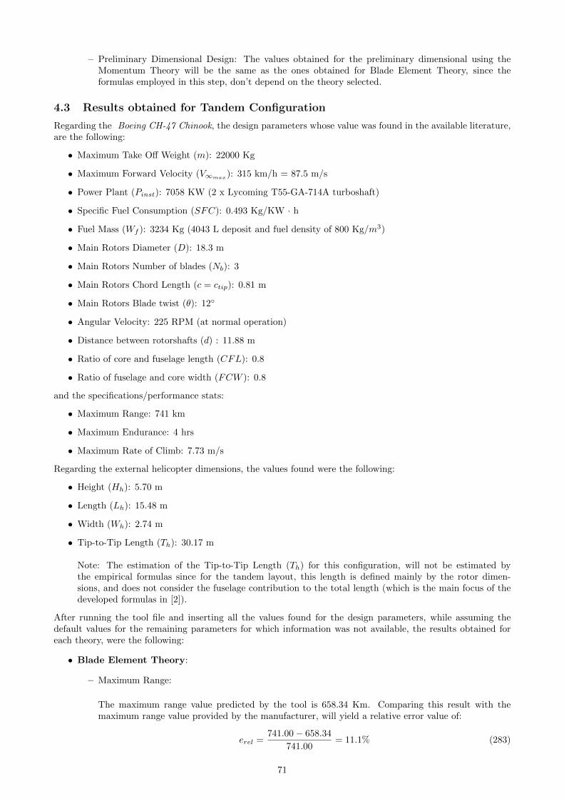
– Preliminary Dimensional Design: The values obtained for the preliminary dimensional using theMomentum Theory will be the same as the ones obtained for Blade Element Theory, since theformulas employed in this step, don’t depend on the theory selected.
4.3 Results obtained for Tandem Configuration
Regarding the Boeing CH-47 Chinook, the design parameters whose value was found in the available literature,are the following:
• Maximum Take Off Weight (m): 22000 Kg
• Maximum Forward Velocity (V∞max): 315 km/h = 87.5 m/s
• Power Plant (Pinst): 7058 KW (2 x Lycoming T55-GA-714A turboshaft)
• Specific Fuel Consumption (SFC): 0.493 Kg/KW · h
• Fuel Mass (Wf ): 3234 Kg (4043 L deposit and fuel density of 800 Kg/m3)
• Main Rotors Diameter (D): 18.3 m
• Main Rotors Number of blades (Nb): 3
• Main Rotors Chord Length (c = ctip): 0.81 m
• Main Rotors Blade twist (θ): 12
• Angular Velocity: 225 RPM (at normal operation)
• Distance between rotorshafts (d) : 11.88 m
• Ratio of core and fuselage length (CFL): 0.8
• Ratio of fuselage and core width (FCW ): 0.8
and the specifications/performance stats:
• Maximum Range: 741 km
• Maximum Endurance: 4 hrs
• Maximum Rate of Climb: 7.73 m/s
Regarding the external helicopter dimensions, the values found were the following:
• Height (Hh): 5.70 m
• Length (Lh): 15.48 m
• Width (Wh): 2.74 m
• Tip-to-Tip Length (Th): 30.17 m
Note: The estimation of the Tip-to-Tip Length (Th) for this configuration, will not be estimated bythe empirical formulas since for the tandem layout, this length is defined mainly by the rotor dimen-sions, and does not consider the fuselage contribution to the total length (which is the main focus of thedeveloped formulas in [2]).
After running the tool file and inserting all the values found for the design parameters, while assuming thedefault values for the remaining parameters for which information was not available, the results obtained foreach theory, were the following:
• Blade Element Theory:
– Maximum Range:
The maximum range value predicted by the tool is 658.34 Km. Comparing this result with themaximum range value provided by the manufacturer, will yield a relative error value of:
erel =741.00− 658.34
741.00= 11.1% (283)
71
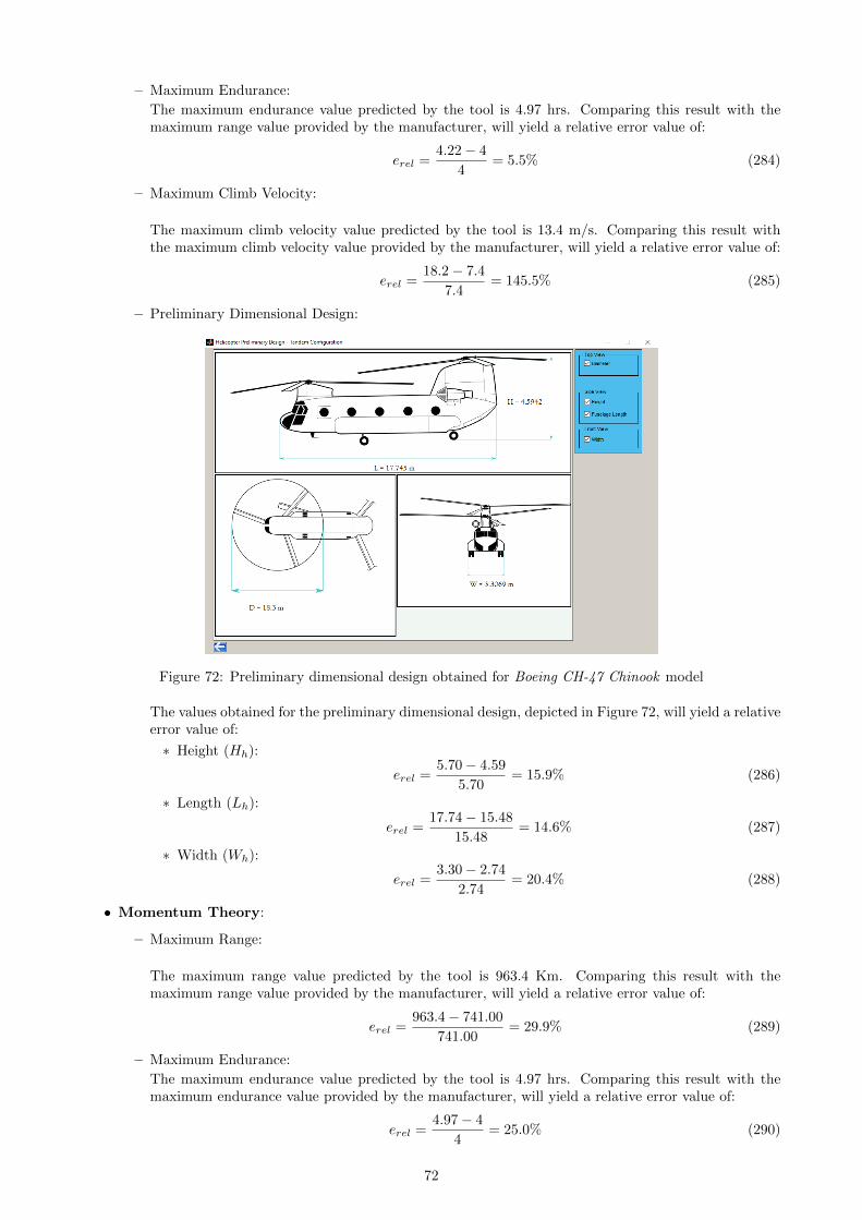
– Maximum Endurance:
The maximum endurance value predicted by the tool is 4.97 hrs. Comparing this result with themaximum range value provided by the manufacturer, will yield a relative error value of:
erel =4.22− 4
4= 5.5% (284)
– Maximum Climb Velocity:
The maximum climb velocity value predicted by the tool is 13.4 m/s. Comparing this result withthe maximum climb velocity value provided by the manufacturer, will yield a relative error value of:
erel =18.2− 7.4
7.4= 145.5% (285)
– Preliminary Dimensional Design:
Figure 72: Preliminary dimensional design obtained for Boeing CH-47 Chinook model
The values obtained for the preliminary dimensional design, depicted in Figure 72, will yield a relativeerror value of:
∗ Height (Hh):
erel =5.70− 4.59
5.70= 15.9% (286)
∗ Length (Lh):
erel =17.74− 15.48
15.48= 14.6% (287)
∗ Width (Wh):
erel =3.30− 2.74
2.74= 20.4% (288)
• Momentum Theory:
– Maximum Range:
The maximum range value predicted by the tool is 963.4 Km. Comparing this result with themaximum range value provided by the manufacturer, will yield a relative error value of:
erel =963.4− 741.00
741.00= 29.9% (289)
– Maximum Endurance:
The maximum endurance value predicted by the tool is 4.97 hrs. Comparing this result with themaximum endurance value provided by the manufacturer, will yield a relative error value of:
erel =4.97− 4
4= 25.0% (290)
72

– Maximum Climb Velocity:
The maximum climb velocity value predicted by the tool is 19.1 m/s. Comparing this result withthe maximum climb velocity value provided by the manufacturer, will yield a relative error value of:
erel =19.1− 7.4
7.4= 158.0% (291)
– Preliminary Dimensional Design: The values obtained for the preliminary dimensional using theMomentum Theory will be the same as the ones obtained for Blade Element Theory, since theformulas employed in this step, don’t depend on the theory selected.
4.4 Results obtained for Co-axial Configuration
Regarding the Kamov Ka-27 model, the design parameters whose value was found in the available literature,are the following:
• Maximum Take Off Weight (m): 12000 Kg
• Maximum Forward Velocity (V∞max): 270 km/h = 75 m/s
• Power Plant (Pinst): 3320 KW (2 x Isotov TV3-117V)
• Specific Fuel Consumption (SFC): 0.308 Kg/KW · h
• Fuel Mass (WF ): 1959 Kg (2449 L deposit and fuel density of 800 Kg/m3)
• Main Rotors Diameter (D): 15.8 m
• Main Rotors Number of blades (Nb): 3
• Main Rotors Chord Length (c = ctip): 0.44 m
• Ratio of boom and fuselage length (BFL): 0.2
• Ratio of boom and fuselage width (BFW ): 0.6
and the specifications/performance stats:
• Maximum Range: 900 km
• Maximum Endurance: 4.5 hrs
• Maximum Rate of Climb: 12.5 m/s
Regarding the external helicopter dimensions, the values found were the following:
• Height (Hh): 5.40 m
• Length (Lh): 11.38 m
• Width (Wh): 3.70 m
• Tip-to-Tip Length (Th): 12.15 m
After running the tool file and inserting all the values found for the design parameters, while assuming thedefault values for the remaining parameters for which information was not available, the results obtained foreach theory, were the following:
• Blade Element Theory:
– Maximum Range:
The maximum range value predicted by the tool is 1218 Km. Comparing this result with the maxi-mum range value provided by the manufacturer, will yield a relative error value of:
erel =1218− 900.00
900.00= 35.3% (292)
73

– Maximum Endurance:
The maximum endurance value predicted by the tool is 5.01 hrs. Comparing this result with themaximum range value provided by the manufacturer, will yield a relative error value of:
erel =5.01− 4.5
4.5= 11.3% (293)
– Maximum Climb Velocity:
The maximum climb velocity value predicted by the tool is 17.48 m/s. Comparing this result withthe maximum climb velocity value provided by the manufacturer, will yield a relative error value of:
erel =17.48− 12.50
12.50= 4.6% (294)
– Preliminary Dimensional Design:
Figure 73: Preliminary dimensional design obtained for Kamov Ka-27 model
The values obtained for the preliminary dimensional design, will yield a relative error value of:
∗ Height (Hh):
erel =5.40− 4.15
5.40= 23.1% (295)
∗ Length (Lh):
erel =15.19− 11.38
11.38= 33.2% (296)
∗ Width (Wh):
erel =3.70− 2.98
3.70= 19.1% (297)
∗ Tip-to-Tip Length (Th):
erel =15.80− 12.15
12.15= 30.1% (298)
• Momentum Theory:
– Maximum Range:
The maximum range value predicted by the tool is 900 Km. Comparing this result with the maximumrange value provided by the manufacturer, will yield a relative error value of:
erel =1214− 900
900= 34.8% (299)
74

– Maximum Endurance:
The maximum endurance value predicted by the tool is 7.09 hrs. Comparing this result with themaximum endurance value provided by the manufacturer, will yield a relative error value of:
erel =7.09− 4.5
4.5= 57.5% (300)
– Maximum Climb Velocity:
The maximum climb velocity value predicted by the tool is 19.7 m/s. Comparing this result withthe maximum climb velocity value provided by the manufacturer, will yield a relative error value of:
erel =19.7− 12.5
12.5= 18.7% (301)
– Preliminary Dimensional Design: The values obtained for the preliminary dimensional using theMomentum Theory will be the same as the ones obtained for Blade Element Theory, since theformulas employed in this step, don’t depend on the theory selected.
All the results obtained are summarized in the following tables:
Model Range Endurance VcBell 429 10.7 % 7.4 % 12.9 %Boeing CH-47 11.1 % 5.5 % 145.5 %Kamov Ka-27 35.3 % 11.3 % 4.6 %
Table 2: Errors obtained with Blade Element Theory
Model Range Endurance VcBell 429 16.4 % 6.2 % 9.8 %Boeing CH-47 29.9 % 25.0 % 158.0 %Kamov Ka-27 34.8 % 57.5 % 18.7 %
Table 3: Errors obtained with Momentum Theory
Model 429 CH-47 Ka-27Hh 8.3 % 15.9 % 23.1 %Lh 9.9 % 14.6 % 33.2 %Wh 13.5 % 20.4 % 19.1 %Th 1.9 % - 30.1 %
Table 4: Errors obtained with empirical formulas developed in [1], which are independent of the theory used
4.5 Discussion of Results
Analyzing the results obtained, it is possible to conclude that the tool is predicting accurately many of thegeneral preliminary design characteristics, for a given set of the desired design parameters. Although the 3models chosen to test the tool accuracy, had several input parameters available, there were still some keyinformation that was lacking, such as the airfoil shape, or the sweep back angle of the blades. However,even with this lack of information, the results obtained showed good agreement for each configuration and foreach theory. The only exception was the maximum climb velocity obtained for the tandem. For this heavyconfiguration (WGTOW > 20000 Kg), the results were not satisfactory. The explanation for this deviance can berelated to the fact that the only constraint implemented in the tool for the maximum rate of climb is the poweravailable, for each forward velocity value. In a heavy rotorcraft, other constraints can play a role such as theones coming from aerodynamic, structural or engine transmission issues, that impose a limit in the maximumrate of climb. Furthermore, since equation (68), used to estimate the value of the interference factor, kov, wasbased on the assumption that the two rotors would be located on the same plane, and since this is not verified
75

for the Chinook CH-47 model (due to its rotor and fuselage dimensions) this fact could have also contributedto the high deviance verified.Regarding the empirical formulas for dimensional design developed by [1], they produced relatively accurateresults for the 3 configurations, even though they were just developed for the conventional configuration. In ageneral analysis these formulas can be used to estimate the dimensions for any new design with conventional,co-axial or tandem configuration.Another issue that must be mentioned is the comparison between the results obtained with the two differenttheories. The Blade Element Theory shows a global tendency for producing more accurate results. This isexpected, since this theory presents much more complexity and an higher number of input variables. However,in some cases, the gain in accuracy does not compensate the increase in the computational time requiredto perform the calculations, when compared with Momentum Theory. For instance, the computational timerequired for Momentum Theory never exceeds the value of 10 seconds, as opposed to Blade Element Theory,which for a number of azimuthal and radial discretization segments greater than 60, can reach up to the 36000seconds. This is not sustainable if the user wishes a quick analysis. Therefore, if the user desires a very fast andbasic analysis, the choice should be the Momentum Theory interface. If the user wishes a more refined analysis,but still with fast results, the choice should be the Blade Element Theory interface, but with a relatively smallnumber of azimuthal and radial discretization segments (<30). For a very accurate analysis the user shouldrefer to the Blade Element Theory interface but knowing that a number of radial and azimuthal discretizationsegments greater then 60, can push the computational time value to several hours.In a general analysis, the tool has accurately predicted the characteristics of the 3 known designs (one for eachconfiguration) even though there were a wide variability of design parameters and characteristics inputted in the3 different designs. This fact increases the confidence that the tool is able to produce accurate and trustworthyresults for any new and experimental design that the user wishes to study/analyze.
76

5 Conclusions
5.1 Achievements
The main goal of this thesis was to develop a complete, user-friendly and trustworthy computational tool thatwould aid the student, researcher or curious in the preliminary design of any new rotorcraft. With this purpose,it was developed a MATLAB tool, simply to use and, at the same time, able to incorporate a wide variety ofinput parameters. The code implementation was done based on the two most famous theories in the rotorcraftfield: Momentum Theory and Blade Element Theory. To evaluate if the tool was predicting accuratetly therotorcraft characteristics, for a given set of input parameters, three helicopter models already developed wereselected (one for each configuration). Using the design parameters values provided by the manufacturers, andinputting this information in the computational tool, the simulations were launched. The results obtainedshowed a relatively good agreement between the predictions of the tool and the real performance characteristicsof the selected models. This fact increases the confidence that the tool developed is able to predict correctlyany new design desired by the user, for the 3 different configurations.
5.2 Future Work
Although the tool has shown good results, some improvements should be made. The computational timerequired for the Blade Element Theory calculations when the number of discretization segments is high, mustbe decreased. Even if the increase in accuracy is not worth the increase in the total required time for thecomputations, the user should have the possibility to refine the results as he wishes without having to waitfor several hours. Nowadays, there are acceleration methods for computational tools, that can be implementedin order to decrease the required time, but their implementation is not straightforward and the results candepend greatly on the code structure. Regarding the tool functionalities, more airfoils and airfoil data shouldbe incorporated, and the possibility to select between several linear inflow models should be included togetherwith the option to choose between different numerical integration schemes. Also, the possibility to performpreliminary structural analysis and stability studies should be included. Furthermore, to make the tool developeda reference for any rotorcraft design, it should be also expanded for preliminary multi-rotor drone design,together with the implementation of an electrical power plant database, similar to the combustion engines database.
77

6 Bibliography
• [1] Rand Omri, Khromov Vladimir, Helicopter Sizing by Statistics, Faculty of Aerospace Engineering,Technion – Israel Institute of Technology, Haifa, 2002.
• [2] http://www.johnson-aeronautics.com/CAMRADII.html. Visited on: 03-03-2016
• [3] Program development for Preliminary Design Helicopter, School of Aerospace, Mech. Manufacturing& Eng., RMIT University, VIC, 3001, Australia, AERO2365 Thesis / Project 2005
• [4] Vasyliovych Rutskyy Roman, Desenvolvimento duma ferramenta computacional para projecto prelim-inar do helicoptero de configuracao convencional, Master’s Thesis, Instituto Superior Tecnico, Lisboa,2014
• [5] Cojocari Anatol, Preliminary design tool of conventional/coaxial/tandem helicopters, Instituto Supe-rior Tecnico, Master’s Thesis, Lisboa, 2016
• [6] Leishman J. Gordon, Principles of Helicopter Aerodynamics, Cambridge Aerospace Series, 2002.
• [7] Rankine W. J. M., On the Mechanical Principles of the Action of Propellers, Transactions of theInstitute of Naval Architects, 6, 1865
• [8] Froude R. E., On the Part Played Propulsion by Differences of Fluid Pressure, Transactions of theInstitute of Naval Architects, 30, 1889
• [9] Lanchester F.W., A Contribution to the Theory of Propulsion and the Screw Propeller, Transactionsof the Institute of Naval Architects, 57, 1915
• [10] Betz, Development of Inflow Theory of the Propeller, NACA TN 24, 1920
• [11] Glauert, Airplane Propellers, In Division L of Aerodynamic Theory, 1935
• [12] Harris, F.D. Twin Rotor Hover Performance, J. of the American Helicopter Soc., 44(1), pp 34-37,1999
• [13] Johnson Wayne, Helicopter Theory, Princeton University Press, 1980
• [14] Froude, W. On the Elementary Relation Between Pitch, Slip and Propulsive efficiency, Transactionsof the Institute of Naval Architects, 1878
• [15] Drzewiecki, S. Theorie Generale de l’Helice, Gauthier-Villars et cie, Paris, 1920
• [16] Brotherhood, P. and Stewart, W. An Experimental Investigation of the Flow through a HelicopterRotor in Forward Flight, Report ARC R&M 2734, Aeronautical Research Council, 1949
• [17] Coleman, R. P., Feingold, A. M., and Stempin, C. W. Evaluation of the Induced Velocity Field of anIdealized Helicopter Rotor, Langley Memorial Aeronautical Laboratory, Langley Field, 1945
• [18] Drees, J.M. A theory of Airflow Through Rotors and Its Application to Some Helicopter Problems,J. of The Helicopter Association of Great Britain, 3(2), July-Sept, pp 79-104, 1949
• [19] Payne, P.R. Helicopter Dynamics and Aerodynamics, Pitman & Sonds, London, 1959
• [20] Pitt, D.M. and Peters, D.A. Theoretical Prediction of Dynamic Inflow Derivatives, Vertica, 5, pp21-34, 1981
• [21] White, F. and Blake, B.B. Improved Method of Predicting Helicopter Control Response and GustSensitivity, 35th Annual Forum of the American Helicopter Soc., Washington DC, May 21-23,1981
• [22] Howlett, J.J. 1981. UH-60A Blackhawk engineering Simulation Program: Vol.1 - Mathematical Model,NASA CR-66309, 1981
• [23] Gessow, A. and Myers, G. C., Jr 1952. Aerodynamics of the Helicopter, Macmillan Co., 1952 (repub-lished by Ungar Publishing, NY, 1967)
• [24] Sissingh, G. Contribution to the Aerodynamics of Rotating-Wing Aircraft, NACA TM 921, 1939
• [25] Prouty, R.W. Helicopter Performance, Stability and Control, PWS Engineering Publishing, Boston,MA, 1986
78