
DEVELOPMENT OF A MULTI-RESOLUTION PARALLEL...
200
1 DEVELOPMENT OF A MULTI-RESOLUTION PARALLEL GENETIC ALGORITHM FOR AUTONOMOUS ROBOTIC PATH PLANNING By DREW TYLER LUCAS A DISSERTATION PRESENTED TO THE GRADUATE SCHOOL OF THE UNIVERSITY OF FLORIDA IN PARTIAL FULFILLMENT OF THE REQUIREMENTS FOR THE DEGREE OF DOCTOR OF PHILOSOPHY UNIVERSITY OF FLORIDA 2012
Transcript of DEVELOPMENT OF A MULTI-RESOLUTION PARALLEL...

1
DEVELOPMENT OF A MULTI-RESOLUTION PARALLEL GENETIC ALGORITHM FOR AUTONOMOUS ROBOTIC PATH PLANNING
By
DREW TYLER LUCAS
A DISSERTATION PRESENTED TO THE GRADUATE SCHOOL OF THE UNIVERSITY OF FLORIDA IN PARTIAL FULFILLMENT
OF THE REQUIREMENTS FOR THE DEGREE OF DOCTOR OF PHILOSOPHY
UNIVERSITY OF FLORIDA
2012

2
© 2012 Drew Tyler Lucas

3
To my family

4
ACKNOWLEDGMENTS
I would like to first thank my family for their support of my educational journey over
the past 10 years. They have encouraged me beyond any of my expectations allowing
me to achieve goals which originally seemed out of reach. Through their unwavering
encouragement, I have been able to develop into the person I am today.
Next, I would like to express my deep thanks to my advisor Dr. Carl Crane for his
support and guidance throughout my graduate school experience. Without his advice
and counseling, I would not have been able to develop my engineering skills or explore
the unique world of autonomous robotics. I would also like to thank my committee
members, Dr. Antonio Arroyo, Dr. Douglas Dankel, Dr. John Schueller, and Dr. Gloria
Wiens for their support over the years and guidance in the research process. I would
also like to extend my thanks to the Air Force Research Lab at the Tyndall Air Force
Base in Panama City, Florida as well the Office of Naval Research for supporting
CIMAR in its research.
Lastly, I would like to especially thank both my current and past co-workers in the
CIMAR lab. They have given me countless memorable experiences and provided me
with phenomenal support while working on all the fascinating, and sometimes stressful,
projects over the years.

5
TABLE OF CONTENTS
page
ACKNOWLEDGMENTS .................................................................................................. 4
LIST OF FIGURES .......................................................................................................... 8
LIST OF OBJECTS ....................................................................................................... 13
LIST OF ABBREVIATIONS ........................................................................................... 14
ABSTRACT ................................................................................................................... 16
CHAPTER
1 INTRODUCTION .................................................................................................... 18
Background ............................................................................................................. 18
CIMAR Background ................................................................................................ 20 Path Planning ......................................................................................................... 20 Evolutionary Computation ....................................................................................... 22
Reactivity in a Dynamic Environment...................................................................... 26
2 MOTIVATION ......................................................................................................... 29
Modeling a Robotic System .................................................................................... 29 High Order Search Spaces and Reactivity .............................................................. 31
Problem Statement ................................................................................................. 34
3 REVIEW OF LITERATURE .................................................................................... 36
Common Path Planners .......................................................................................... 36
A*/D*/D*Lite ...................................................................................................... 36 Probabilistic Roadmap ..................................................................................... 37
Potential Fields ................................................................................................. 38 Anytime Planners ............................................................................................. 38
Evolutionary Algorithms .......................................................................................... 40
Representation ................................................................................................. 40
Parallel Evaluation ............................................................................................ 42 Genetic Algorithms for Dynamic Optimization Problems ......................................... 45 Genetic Algorithms for Path Planning ..................................................................... 52
Static Environments ......................................................................................... 53 Dynamic Environments..................................................................................... 55 Genetic Algorithm Modifications ....................................................................... 56
4 PREVIOUS RESEARCH ........................................................................................ 61

6
Simplistic Simulation ............................................................................................... 61
Reactive Search ..................................................................................................... 62 Parallel Evaluation .................................................................................................. 63
5 REFINED APPROACH ........................................................................................... 72
Problem Scope ....................................................................................................... 72 Workspace Definition .............................................................................................. 72 Spline Representation............................................................................................. 73
Path Cost .......................................................................................................... 75
Spline Observations ......................................................................................... 76 Spline Calculation and Evaluation .................................................................... 78 Parallel Calculation with OpenCL ..................................................................... 79
Combinatorial Operations ....................................................................................... 83 Bounded Operators .......................................................................................... 84 Globally Bounded Operators ............................................................................ 84
Mutation ..................................................................................................... 84 Inflation ...................................................................................................... 84
Locally Bounded Operators .............................................................................. 85 Mutation ..................................................................................................... 85 Inflation ...................................................................................................... 85
Other Operators ............................................................................................... 85 Deletion ...................................................................................................... 86
Swap .......................................................................................................... 86 Crossover equal ......................................................................................... 86
Crossover random ..................................................................................... 87 Block .......................................................................................................... 87 Fan ............................................................................................................. 87
Perturbation ............................................................................................... 88 Dynamic Population Ratios ..................................................................................... 88
Population Building Blocks ...................................................................................... 89 Anytime Planning with Population Seeding ............................................................. 92
6 EXPERIMENTAL RESULTS ................................................................................. 123
Setup .................................................................................................................... 123 Random Bias ........................................................................................................ 124 Testing Hardware ................................................................................................. 125
Static Convergence .............................................................................................. 126
Small Search Space ....................................................................................... 126 Valley search ........................................................................................... 127 Constrained valley search ........................................................................ 128 Static obstacle search .............................................................................. 129
Large Search Space ....................................................................................... 130
Valley search ........................................................................................... 130 Static obstacle search .............................................................................. 132
Dynamic Convergence.......................................................................................... 133

7
Random Object Insertion ................................................................................ 134
Oscillatory Object Simulation .......................................................................... 135 Deterministic Search Comparison ........................................................................ 135
7 DISCUSSION AND FUTURE WORK ................................................................... 182
Assessment of Fitness to Problem Scope ............................................................ 182 Future Work .......................................................................................................... 182 Conclusions .......................................................................................................... 185
APPENDIX
A EXAMPLE SPLINE CALCULATION ..................................................................... 187
B EXAMPLE TEST MOVIES .................................................................................... 192
LIST OF REFERENCES ............................................................................................. 193
BIOGRAPHICAL SKETCH .......................................................................................... 200

8
LIST OF FIGURES
Figure page 1-1 Genetic Programming Tree example. ................................................................. 28
1-2 Genetic Algorithm Chromosome example .......................................................... 28
3-1 Hyper-mutation application ................................................................................. 60
4-1 Simplistic vector path chromosome .................................................................... 65
4-2 Smoothing and Expansion vector mutation operators ........................................ 65
4-3 Initial population of simplistic vector planning with static obstacles: Trial 1 ........ 66
4-4 Results of simplistic vector planning with static obstacles: Trial 1 ...................... 67
4-5 Cost vs planning time for simplistic vector planning with static obstacles: Trial 1 ......................................................................................................................... 67
4-6 Initial population of simplistic vector planning with static obstacles: Trial 2 ........ 68
4-7 Results of simplistic vector planning with static obstacles: Trial 2 ...................... 69
4-8 Cost vs planning time for simplistic vector planning with static obstacles: Trial 2 ......................................................................................................................... 70
4-9 Dynamic path adjustment for the simplistic vector planner ................................. 70
4-10 Cost vs planning time for the simplistic vector planner using dynamic objects ... 71
5-1 A quad-tree representation of the search space with a single spline intersecting several portions of the tree .............................................................. 95
5-2 The modified search space storage strategy with downscaled grids stored in hashmaps ........................................................................................................... 96
5-3 The representative genome discretization for an individual spline...................... 96
5-4 Spline division example ...................................................................................... 97
5-5 Spline.with knot points and control points labeled .............................................. 97
5-6 Cost equation for a candidate solution ............................................................... 98
5-7 Stratification effect on generated paths .............................................................. 99
5-8 The effect of pooled control points on incremental evaluation .......................... 100

9
5-9 Out of order control point loops ........................................................................ 101
5-10 The effect of the Blocking operator on a spline................................................. 102
5-11 The De Boor method for evaluating a parameterized b-spline curve ................ 103
5-12 The De Boor calculated reduced to matrix form ............................................... 103
5-13 Example resultant of applying the cell occupancy algorithm to a candidate spline solution ................................................................................................... 104
5-14 The modified Bresenham approach to calculate cell occupancy ...................... 105
5-15 OpenCL divisions of processing and memory capacity .................................... 106
5-16 OpenCL device allocation and host interaction................................................. 106
5-17 OpenCL memory buffer indexing ...................................................................... 107
5-18 Timed profiling of test run ................................................................................. 107
5-19 Native conditioning and incrementing of spline ................................................ 108
5-20 OpenCL conditioning and incrementing of spline ............................................. 109
5-21 Cell occupancy using a single thread on the CPU ............................................ 110
5-22 Cell occupancy using a single thread on the CPU ............................................ 111
5-23 Search space exploration and population size ................................................. 112
5-24 Control point inflation in large search areas ..................................................... 113
5-25 Over specification of control points ................................................................... 114
5-26 Example of when deletion operator is appropriate ............................................ 115
5-27 Diagram of equal crossover .............................................................................. 116
5-28 The effect of the blocking operator on a spline ................................................. 116
5-29 The result of the Fan operation of a spline ....................................................... 117
5-30 Appropriate increment counts in low resolution grids ....................................... 118
5-31 High resolution image of the Small Valley sample test area ............................. 119
5-32 A low resolution image of the Small Valley sample test area ........................... 120
5-33 Gene pool strategy for evolutionary building blocks ......................................... 120

10
5-34 Downscaling search space grids ...................................................................... 121
5-35 Mult-resolution genetic path planner processing organization .......................... 122
6-1 Mult-resolution genetic path planner processing organization .......................... 138
6-2 Map of campus test run using the Urban Navigator .......................................... 139
6-3 A 1024x1024 Small Valley search grid ............................................................. 140
6-4 A 8192x8192 Large Valley search grid ............................................................. 141
6-5 A moving object intersecting the low cost valley ............................................... 142
6-6 An exaggerated Gaussian noise mask applied to a small search space .......... 143
6-7 A threshold mask applied to the search grid to focus the search within a desired area...................................................................................................... 144
6-8 A threshold mask applied to the search grid to focus the search within a desired area...................................................................................................... 145
6-9 Evolutionary trials using the different initial populations ................................... 146
6-10 Constrained Valley maze test with the desired solution .................................... 147
6-11 Small Valley trail using a single population ....................................................... 148
6-12 Small Valley trial using 4 seeding threads ........................................................ 149
6-13 Another Small Valley trail using a single population ......................................... 150
6-14 Another Small Valley trial using 4 seeding threads ........................................... 151
6-15 Desired converged solution for the constrained valley search test ................... 152
6-16 Constrained Valley trial using a single population ............................................ 153
6-17 Constrained Valley trial using 4 seeding threads .............................................. 154
6-18 Constrained valley search using the a population at each resolution ............... 155
6-19 The desired minimum cost path for the small search space static obstacle tests .................................................................................................................. 156
6-20 Small Static Obstacle trial with a single population ........................................... 157
6-21 Small Static Obstacle trial with 4 seeding threads ............................................ 158

11
6-22 Small Static Obstacle trial with 7 seeding populations ...................................... 159
6-23 Large Valley desired path ................................................................................. 160
6-24 Large Valley trial using a single population ...................................................... 161
6-25 Large Valley trial using 4 seeding threads ........................................................ 162
6-26 Large Valley trial using a single population with OpenCL ................................. 163
6-27 Large Valley trial using 4 seeding threads with OpenCL .................................. 164
6-28 Large Valley trial using 4 seeding threads with 300 individuals ........................ 165
6-29 Large Valley trial using a single population with 300 individuals ...................... 166
6-30 Large Valley trial using 4 seeding threads with 300 individuals with OpenCL .. 167
6-31 Large Valley trial using 4 seeding threads with 300 individuals with OpenCL .. 168
6-32 A desired path across the large static obstacle sample space ......................... 168
6-33 Large Static Obstacle trial using a single population ........................................ 169
6-34 Large Static Obstacle trial using 4 seeding threads. ......................................... 170
6-35 Large Static Obstacle trial using 4 seeding threads. ......................................... 171
6-36 Large Static Obstacle trial using 4 seeding threads with OpenCL .................... 172
6-37 Random moving object insertion and adjustment ............................................. 173
6-38 Random moving object single population adjustment ....................................... 174
6-39 Random moving object single population-4 seeding thread comparison .......... 175
6-40 Oscillatory object obstructing the low cost valley .............................................. 176
6-41 Oscillatory object obstructing the low cost valley .............................................. 177
6-42 Oscillatory object trial using a single population ............................................... 178
6-43 Oscillatory object trial using 4 seeding threads................................................. 179
6-44 Unconstrained expansion A* example .............................................................. 180
6-45 Node expansion for unconstrained A* .............................................................. 181
6-46 Indexed A* expansion within a small sample search space ............................. 181

12
A-1 De Boor process for parametric evaluations ..................................................... 187
A-2 Division separation for example spline with 5 control points ............................. 188
A-3 Pyramid structure of N value dependencies. .................................................... 188

13
LIST OF OBJECTS
Object page B-1 Sample of the small valley test area ................................................................. 192
B-2 Sample of the constrained valley test area ....................................................... 192
B-3 Large static obstacle test area .......................................................................... 192
B-4 Single dynamic oscillatory object test area ....................................................... 192

14
LIST OF ABBREVIATIONS
AP Anytime Planner
AUV Autonomous Underwater Vehicle
CIMAR Center for Intelligent Machines and Robotics
CPLD Complex Programmable Logic Device
CPU Central Processing Unit
CUDA Compute Unified Device Architecture
DARPA Defense Advanced Research Projects Agency
DBMS Database Management System
DOF Degree of Freedom
DOP Dynamic Optimization Problem
EA Evolutionary Algorithms
EC Evolutionary Computation
EL Epigenetic Learning
FLOPS Floating Point Operations per Second
FPGA Field Programmable Gate Array
GA Genetic Algorithms
GP Genetic Programming
GPS Global Positioning System
GPU Graphical Processing Unit
GUI Graphical User Interface
HLP High Level Planner
IMU Inertial Measurement Unit
LIDAR Light Detection and Ranging
OpenCL Open Computing Language

15
PRP Probabilistic Roadmap Planner
PSO Particle Swarm Optimization
RI Random Immigrants
RRT Rapidly-exploring Random Tree
SLAM Simultaneous Localization and Mapping
UAV Unmanned Aerial Vehicle
VLS Variable Local Search

16
Abstract of Dissertation Presented to the Graduate School of the University of Florida in Partial Fulfillment of the Requirements for the Degree of Doctor of Philosophy
DEVELOPMENT OF A MULTI-RESOLUTION PARALLEL GENETIC ALGORITHM FOR
AUTONOMOUS ROBOTIC PATH PLANNING
By
Drew Tyler Lucas
August 2012
Chair: Carl Crane, III Co-Chair: Antonio Arroyo Major: Mechanical Engineering
Deterministic algorithms such as A* and D* have been applied with great success
to autonomous robotic path planning. However, as search space size increases
numerous problem domains will likely become intractable when reactive behavior is
desired. This is extremely relevant when considering the exponential increase in search
space sizes due to any linear addition of degrees of freedom. Over the last few
decades, evolutionary algorithms have been shown to be particularly applicable to
extremely large search spaces. However, it is often assumed that generational
convergence is the only measure of quality for an evolutionary algorithm. A novel
combination of the Anytime Planning criteria with multi-resolution search spaces is
explored for application to high-level semi-reactive path planning. Separate populations
are evolved in parallel within different abstractions of the search space while low cost
solutions from each population are exchanged among the populations. Generational
evaluations in low-resolution search spaces can be evaluated quickly generating seed
candidate solutions that are likely to speed convergence in the high-resolution search
spaces. Convergence rates up to 4x were achieved along with modest decreases in

17
path cost. Parallel GPU computation was then applied to allow reactive searching up to
40Hz in search grids up to 8192x8192 cells.

18
CHAPTER 1 INTRODUCTION
Over the past half century, robots have emerged from science fiction as real world
entities used pervasively in many facets of everyday life. From the factory floor to more
recent interactive consumer products, robots continue to push the bounds between
science fiction and reality. One exciting area of focus has been autonomous robots and
their applications. While most development has gone into robots for military uses, the
research involved and subsequent robotic development can be applied to many areas
of interest.
Background
The desire to create tools which complete tasks with little or no human intervention
has been prevalent for as long as humans have used tools. Tools which can operate
with no human intervention are generally classified under the field of automation. These
automatic tools can further be split into two groups: those that adjust their function
based on feedback from the work environment and those that do not. Robotics fits into
the first of these two categories with the use of sensor and reactive control
methodologies.
A historical survey of robotics is difficult because their classification is not exact. A
robot is defined as an autonomous device which can function with human like behavior.
However, classifying behavior is a largely qualitative and subjective measure. It could
be argued that any feedback system has some intelligence because it may react to
stimulus much as a human would. In this paper, an autonomous robot is defined as a
machine that is able to negotiate movement within its environment while maintaining
user specified constraints without human interaction.

19
Automatic machines in general saw a dramatic increase in use with the advent of
the industrial revolution. More and more industrial practices saw automatic machines
take the place of skilled human laborers in traditionally human work areas. These
inventions included the automatic cotton picker and processor as well as the almost
complete replacement of humans in cloth production by the 19th century. The machines
were able to interact with their environments in that they operated on physical materials
but did not have intelligent feedback systems in place more than rudimentary speed and
position control.
The first practical steps towards seemingly autonomous behavior were expanded
upon with Tesla’s invention of a teleoperated torpedo and boat for the US military.
Tesla outfitted a boat for remote control by creating a system that would wirelessly
beam commands to a receiver, something that may be commonplace today but was
revolutionary just a century ago. This was a radical step in the process of automation
as it created a sense of reaction without human intervention. Bystanders first caught a
glimpse of seemingly intelligent, controllable behavior without any physical link to the
machine. This advancement spurred the interest into realizable machines which would
act as a human would even though it still needed control inputs from a human to
operate.
Within the past 30 years autonomous robotics has seen larger and larger gains
towards the goal of real cognition and capable human level interaction. As experiments
move from small robots in the lab to more capable systems applied to real world
problems, autonomous robots now seem fit to address many of the problems humans

20
will encounter in the future. Even with all these strides in robotic development, many
areas still need to be addressed.
CIMAR Background
CIMAR’s work in autonomous vehicles started in the 1980s and 1990s with work in
ground vehicles for the Air Force. Several autonomous ground vehicles were created
for use in runway repair and area clearance. With the advent of the DARPA ground
vehicle competitions 10 years ago, a major drive within the lab has been intelligent
ground vehicles which can travel on roadways and through urban environments. This
work culminated in the entries into the DARPA grand challenges and subsequent
DARPA urban challenge. While not winning these competitions, much development
has gone into creating robust robotic systems which can successfully navigate through
roadway environments. Recent work has continued into autonomous ground vehicles in
both area coverage and mapping for unexploded ordinance along with area clearance
and vegetation removal. Several different autonomous platforms are available for
experimentation with varying levels of computational capabilities and sensor packages.
Path Planning
One of the basic features of an autonomous robot is the ability for it to move from
location to location within an environment. This operation is usually abstracted into two
separate actions: creating a desired path and generating the control inputs to cause the
physical robot to move within its environment. To find a suitable path for the robot to
move through, the robot must know information about how it is spatially oriented, how it
can move through its environment and what else is in the environment.
The first piece of information, finding a current spatial orientation, can be divided
into two different instances. For non-reconfigurable robots, the size and shape are

21
usually a prior knowledge that does not change within the scope movement. However,
the orientation and position within its environment will hopefully change with time. This
information can be obtained through the use of GPS or other localization techniques
such as SLAM or IMU sensors. A robot must know its position, or at least an
approximation of its position, to estimate whether it is behaving as designed.
Secondly, the robot must know how its movements will affect its position and
orientation through time. For holonomic robots, a simple control input can usually
generate a direct movement from a start position to and end position. However, for
non-holonomic robots like automobiles, reachable configurations can be much more
difficult to find. Turning radius is a prime factor in finding drivable paths for many
ground vehicles. This idea has often been further abstracted by using the idea of screw
theory to combine the steering angle with the desired speed to classify the configuration
state of the vehicle at any one time. Various optimization or search algorithms can
then be used to generate a series of reachable configurations so that the desired
behavior is executed.
The last information is usually gathered with sensor technology so that an
accurate portrayal of the robot’s surroundings can be built. Autonomous robots have
used a wide variety of sensors ranging from cameras to tactile sensors to expensive
LIDAR systems. Artificial information can also be inserted into this world model view so
that operators can guide the robot to behave in a certain manner.
With these three attributes, autonomous robots can create control feedback
systems to actively navigate through dynamic environments. A path is generated,
commands are executed to move the robot through its environment, and its situation is

22
evaluated through sensor feedback. Adjustments can then be made to the control input
to keep the robot on the desired course or the path could change if the environment
around the robot requires it. It should be noted that re-evaluation of the path is
especially important when designing a system that can react to environmental changes.
While differing methods have been implemented with varying success, path planning
still serves as an active research field filled with fascinating correlations to optimization
and numerous other areas of interest.
Evolutionary Computation
Evolutionary computation (EC) was developed as a way to use biological theories
to solve problems. The methods employed in this branch of study work by mimicking
the concepts involved in evolutionary biology by replicating the idea of survival of the
fittest. They have been adapted across many different problem domains but generally
relate to situations in which some sort of optimization occurs. While the basic idea of
EC is very straightforward, complex problems have been solved faster and more
efficiently than many other strategies.
In its most simplistic form, a population of solutions is generated and iteratively
forced through many generations while applying a fitness evaluation to each solution to
determine if any portion of that solution will reach successive generations of solutions.
The fitness of a solution is generally how well it approximates the desired solution.
Good solutions will then ‘breed’ or combine portions of their makeup with other good
solutions within the population to form the next generation of solutions. A wide variety
of additions and modifications have been made to EC methods such as mutation and
crossover which are discussed later.

23
While the terms used to describe evolutionary computational methods are
sometimes mixed and matched depending on the intent of the designer, EC can usually
be divided into two main classes of study: Programming and Algorithms. Evolutionary
or Genetic Programming usually refers to methods which allow the solution fitness
evaluation to evolve. The following example is commonly used to represent a simplistic
implementation of a GP optimization.
A tree structure is first defined so that nodes of the tree represent addition,
subtraction, multiplication, or division. The leaf nodes represent numeric values. The
objective of the program is to find a solution tree that will generate a certain number with
the least possible operations. The tree is evaluated by starting at the leftmost leaf node
and recursively applying the specified operation of the leaf’s parent node with the sibling
nodes. An example of such a tree is shown in Figure 1-1.
First, a population of solutions is randomly generated. This is a very important
aspect of most evolutionary computations because the goal of the procedure is to
eliminate any bias the designer has in deciding what is important for a solution.
Randomly choosing possible solutions allows the evolutionary processes to overtake
any design bias inherent in the implementation processes. This does not mean the
system designer has no influence on the evolutionary process. Values such as the
desired population size and individual program size need to be set or tuned according to
domain specific knowledge and platform restrictions. The randomized population is
then iterated upon using evolutionary concepts until a threshold of fitness is met.
On the other hand, algorithms generally relate to a static method of computing the
fitness of a candidate solution. The common method of representation is a linear

24
genome with each chromosome representing some value used to calculate the fitness
of the individual. This is more in line with how genetic information is represented in
nature with complex molecules forming the building blocks of the genetic code. The
previous problem that was dealt with using GP can be optimized using GA as well. In
this example, an individual chromosome would represent a pairing of operator and
number as illustrated in the example shown in Figure 1-2. The operators are
consistently applied to each gene depending on its location in the chromosome. A set
of these genes would represent the chromosome for an individual in the population.
The chromosome would be evaluated by iteratively picking off genes and applying the
mathematical operator to the previously calculated value and the number contained in
the individual gene.
The evolutionary concepts are applied similarly in GA as they are applied to GP.
A random population of individuals is generated, genetic operations are applied to the
individuals, and a new population is formed for each generational iteration. This
process is repeated until a solution is found or some threshold for correctness is
reached.
It is important to note that EC methods are not guaranteed to find a solution.
They are called probabilistically complete in that given enough time, the probability that
a solution is not found decreases to zero. Even when a solution is found for a specific
problem set, the solution is not guaranteed to be optimal. Solutions may converge to
local optima and may not move from it. This differs from other heuristic search methods
such as A* wherein given enough time and memory, and when using admissible
weightings, an optimal solution, when one exists, will be found. However, EC has been

25
applied to a varied array of problem sets with dramatic results. The reason why EC
produces solutions from seemingly random guessing has been studied by John Holland
in the 1970s. Holland’s Schemata Theorem attempts to describe a reason why EC, and
GA in particular, seem to form better solutions to a problem over successive
generations. Most of the techniques described by EC methods are found through trial
and error rather than a pure mathematical rationale.
The study of EC methods is divided into theory and application. Those that study
EC in theory usually use similar mathematical optimization problems to try to simulate
how a method will function within a certain problem set. For example, to judge a new
modification of the GA for dynamic environments, the dynamic knapsack problem is
simulated. The experimenter usually makes many tests by adjusting parameters such
as population size and rates of mutation to see if their new methods can adjust better to
changes in the environment better than previous dynamic GA systems. Many
interesting complexities have been found in EC methods through these simulations
including different representation abstractions as well as self-adapting behavior.
In contrast to this theoretical approach, EC is often applied to real world systems.
These problems often include complexities that are very hard to model with exact
mathematical theory. This usually causes deviations from traditional EC methods
through the use of domain specific modifications which aid in solution finding. There is
often a tradeoff, as is seen in many real world solutions, between creating general
systems which can be applied to many problems and tailoring a method to fit the needs
of the problem at hand.

26
Reactivity in a Dynamic Environment
The vast majority of mobile robots need to react to their environments so that
desired behaviors can be executed. Reactivity can relate to a static instance of the
world around the robot or a dynamic, constantly changing model that needs to keep an
up to date view of the world. In relation to path planning, using static verses dynamic
world models can drastically alter the way the planning algorithm will operate. When
using a static model, a single path can be generated offline before the robot even
moves. The robot will then try to execute commands to cause the robot to stay along
this course and path planning simply becomes an optimization problem. However,
when dynamic information is used, multiple plans may need to be generated during
runtime and considerations need to be made as to when re-planning should occur along
with what the physical operation of the robot should be during this interim.
One simple method commonly used to deal with dynamic data is to re-plan the
robot’s path whenever new data becomes available. This method seems logical
considering more efficient paths may be found when new data about the robot’s
environment becomes available. It is more robust than trying to classify whether the
path should be regenerated. However, by ignoring the possibility of the current path
staying as the most efficient path, this method will add additional computation to the
system, possibly unnecessarily.
In converse to the above method, algorithms such as the traditional D* approach
path planning by only re-planning in dynamic environments when the currently planned
optimal paths becomes blocked or a cost threshold is exceeded. This becomes much
more computationally efficient as only the generated path needs to be reevaluated
instead of being regenerated with a full search. This method has been used on highly

27
risk adverse projects such as the Mars Explorer robots with much success. However, it
works best when sensor data is not noisy or inaccurate. When this is the case, it may
take more time to re-plan with this method than simply continually re-planning as with
the previous method because the extra step of path evaluation must be done at every
iteration.

28
Figure 1-1. An example of Genetic Programming. Each inner node in the tree structure
represents a numeric operation while each leaf node represents a number. The evaluation of the tree is given as shown at the bottom of the figure.
Figure 1-2. An example of Genetic Algorithms. Each gene represents a static portion
of the fitness evaluation function. A collection of genes represents a chromosome. The chromosome then represents an individual in the evolutionary population. The example evaluation of the given chromosome is given at the bottom of the figure.

29
CHAPTER 2
MOTIVATION
Modeling a Robotic System
A traditional approach to designing a robotic system is to use how the human
thinks as a basis for modeling various components for the system. For instance, the
abstraction of sensor data to objects is a major drive in robotics research. This route
seems logical as that is what humans do intuitively while interacting with their
surroundings and is a good starting point for make an autonomous agent. An example
would be to use a LIDAR line scan to classify whether the reflected points are a car or a
tree by comparing relative distances or some measure of point concentration.
This methodology has seen many impressive demonstrations which reinforce the
validity of abstraction and the subsequent deterministic interpretation of that data.
Numerous instances of autonomous systems have been created which rely on data
collected from various sensors such as LIDAR and cameras. This data is then
classified using any number of reliable, well defined algorithms which allow abstractions
to be created from the raw sensor data. Camera images can be processed through
filters to judge relative color density to find specific objects within a viewing scene.
LIDAR point data can be stitched together to form predictions as to whether the point
strikes correspond to a single object or a set of multiple objects. These abstractions
can then be fed into planning and cognition software which make the robotic platform
complete some desired task.
The shortcomings of this approach are seen when considering the situation
where sensor data is not reliable in that there is oscillatory data (which is commonly
seen in LIDAR applications), noisy data (which can be prevalent in camera systems), or

30
unexpected data. System designers can approach the first two problems by either
procuring better sensor systems or by filtering the captured data. The first mitigation
technique is not always viable considering the small budgets usually required for
implementation of autonomous systems. The use of data filtering only costs
computational resources which is usually preferred because it is cheaper and only
requires time to develop and test the filtering algorithms.
However, by relying on abstractions within the system architecture, designers
need to worry about how well those abstractions can be created relative to what is
expected. This idea is also relative to instances where unexpected situations are
observed. Statistical processes have been formulated, such as the Kalmen filter, which
attempt to generate approximations as close to the ‘real’ value as possible. For many
applications this is perfectly appropriate. Much success has been achieved in the
various fields of application.
With the DARPA Grand Challenge and DARPA Urban Challenge, CIMAR has
taken the approach of designing a receding horizon A* search methodology to solve the
reactive path planning problem. This method finds the most efficient path, within the
scope of the robot’s local world model, to a projected goal point located at the horizon of
the local world model. In this instance, the world model was abstracted into a grid of
cells with each cell representing the relative traversability of the region it enclosed. The
candidate path’s fitness, or relative cost, was then evaluated by adding the costs of
each cell the path intersects in the grid. The grid resolution and dimension was found
experimentally by varying these values until the software was able to produce paths
within a certain time step which was defined as being reactive to its environment. The

31
path was then re-planned continuously as the robot moves and when sensor
information was updated. Another, high level planner (HLP) was used to generate the
goal points for the lower level planner to follow. This HLP made use of a high level
abstraction of all the a priori information about the environment the robot traveled
through along with an A* search to find optimal connections through the graph.
Whenever a significant change to the a priori information was found, a system of
re-plan requests was implemented so that a new HLP plan could be generated. This
added to the complexity of the system but did achieve the intended purpose of creating
movements that were observed as intelligently reacting to the problem while still
following mission parameters.
High Order Search Spaces and Reactivity
Several problems are not addressed with the above approach which will likely
plague autonomous systems in the future. The overall goal of the autonomous system
is to preserve consistent reactivity within varied environmental conditions while still
maintaining mission objectives. This requires a plan to be generated in the robot’s
configuration space within some timeframe. The previous approach is constrained to a
certain amount of search area before reactivity starts to decline. The other issue is that
of abstraction. As the amount of information in robotic systems is likely to increase in
the future, as well as the sources from which they come, for the above approach it
would be important that the information be consistently abstracted. All of these issues
revolve around information which brings up a fundamental question: what happens
when the amount of information an autonomous platform must deal with increases?
One way of dealing with this influx of data is to increase computational
resources. Many planning algorithms can scale proportionally with increases in

32
execution time and storage space. It is important to keep performance consistent to
duplicate reactivity no matter what sensor or other informational sources are used to
create a world model. One prominent example of this can be seen in so called cloud
computing. In this architecture, hardware is completely abstracted and performance of
a certain process is scaled as their load increases as desired. Similar approaches have
been taken with autonomous platforms by adding extra compute nodes or increasing
resources on the computers that run the processes. However, it is hard to tell if
demands on computational resources will scale in proportion to the needs of future
autonomous platforms.
Various methods of caching and parallelism have also been exploited alongside
advancements in computing power to keep algorithmic performance consistent while
the amount of information needing to be processed has intensified. For example, a
simple A* search algorithm may run out of memory after expanding a certain amount of
nodes before the goal is found. One way of continuing the search would be to simply
write a portion of the nodes to disk so they can be explored later if needed. This is
similar to what common Database Management Systems (DBMS) do routinely and
many strategies of how to manage the transactions have been developed to promote
optimality. Still, this will slow down the overall execution of the algorithm because writes
to disc are generally more time consuming than memory access. Implementation
details such as this are not necessarily guaranteed to relate to the ability of a planning
scheme to scale with increasing informational load but can be generally shown to do so
for many systems.

33
Parallelism has also been exploited in recent years to increase efficiency for many
algorithms. Although performance gains are usually tied to the specific problem domain
and algorithm being parallelized, much research has gone into scheduling and memory
sharing approaches which have the ability to increase performance over traditional
linear processing by orders of magnitude. A simplistic application to the A* method
would be to evaluate several node expansions in parallel. This approach may speed up
the overall execution time of the algorithm depending on how it is implemented on the
computer hardware. Recent advances in general purpose computation on graphical
processor units has increased interest with consumer level parallel processing
techniques and has been applied to many autonomous robotic platforms.
Even with these improvements in computing, classical methods of search may
not be able to keep up as data loads increase. It is a fairly reasonable approximation
that information gained from higher resolution sensors and other sources such as
remote databases will increase exponentially in the coming years. Constraining search
spaces through artificial filtering and classification is always one possible way to deal
with increasing information. As mentioned previously, another way would be to
increase algorithmic efficiency or computational resources. One more possibility, which
is the focus of this research, is the use of algorithms such as evolutionary computation
which are nondeterministic but have been shown efficient at exploring very large search
spaces. It is generally accepted that for the majority of problems, the search space size
will increase exponentially with the dimension of the search space leaving methods like
A* impractical while encouraging the use of probabilistic complete methods.

34
Using nondeterministic search for an autonomous platform may seem counter
intuitive at first because of the obvious safety concerns that are involved with moving
robots. In some cases, an operator will want to know exactly how the platform will react
to a certain stimulus. However, using EC methods may be an efficient way to deal with
the exponentially increasing data loads that are likely as autonomous robotics continue
to develop. EC is by no means the only probabilistic methodology which can be applied
to path planning which will be seen in the literature review. It does, however, offer an
interesting solution to the path planning problem which is likely to hold back
advancement of future robotic platforms.
Problem Statement
In this research, the goal of a path planner is defined as finding a viable path from
a start location to an end location within a search space. Viability is to be judged on
platform specific criteria. It is generally accepted that larger search spaces will become
prevalent as richer sensor data becomes available to autonomous platforms. This
sensor data, in combination with other parameters such as possible variable robotic
configurations and orientations, will increase search space dimensionality and size.
Traditional path planning algorithms may not scale uniformly with increasing
computational resources especially when considering the algorithm must generate a
plan that reacts to a dynamic environment. The objective of this research is to use
Genetic Algorithms and evolutionary computation concepts to address the problems
noted in the previous discussion while maintaining platform reactivity. A path plan
needs to be generated that represents a solution that the platform can physically realize
in a relatively unstructured environment. As Evolutionary Optimization is not
guaranteed to converge to the optimal solution within a specific time, the idea of an

35
anytime planner will be evaluated in contrast to deterministic path planning optimization.
Parallelized computation will be used to facilitate cost calculations.

36
CHAPTER 3
REVIEW OF LITERATURE
Common Path Planners
Many methods have been used to solve the path planning problem in robotics.
Some are directly influenced from graph theory while others stem from solving the path
planning problem in robots. While varied in approach, the planners can be separated
into two major categories: deterministic and nondeterministic. Determinism in a planner
at first seems like a requirement but nondeterministic planners are still useful if they are
probabilistically complete. This means that given enough time the chances that the
planner will not find a solution decrease to zero. A general overview of planners will first
be given with a concentration on probabilistic planners.
A*/D*/D*Lite
The most widely used method in robotic path planning is likely to be the A*
method. It is generally used because of its guaranteed optimality when using
admissible conditions and a simplistic design which can easily be implemented and
tuned. CIMAR has used this search method extensively for several projects with
consistent results [1], [2]. D* is a modification of A* search and stands for Dynamic A*.
As the name suggests, it provides for a better method of dealing with dynamic
environments by building a search from the goal node back to the start node in a graph
[3]. When a change is detected that invalidates the best path, portions of the graph are
reevaluated by using previously but reevaluated nodes in the search. Various methods
have been introduced to supplement this approach such as Focused D* which adds
heuristic costs to the expansion steps to reduce the amount of nodes needing to be
evaluated [4]. Many modifications of the traditional A* methods have been attempted

37
such as localized elastic bands for obstacle avoidance [5] and incremental adaptive
heuristic changes [6] which improve path generation times and quality.
Probabilistic Roadmap
A probabilistic roadmap planner (PRP) generates a network of connected
configurations through a search space which are subsequently sampled with local
search methods to find solutions. The planning operation is generally separated into
two phases. The construction phase is first where the search space is randomly or
specifically sampled and the configurations are joined together with collision-free
movement. The second phase is the query phase where the previously constructed
roadmap is searched for an optimal path from a start to a goal node. The roadmap can
be queried multiple times and in multiple locations if the start and end configurations
can be linked to nodes within the roadmap. Like EC, no guarantee of optimality is given
because the search space is sampled instead of wholly evaluated. Many problems still
exist with using PRPs which can have problems with constrained optimality (corridors)
and may take time to generate roadmaps within the search space depending on its size
and dimensionality.
The way in which the space is sampled can have dramatic effects on efficiency
with PRPs. In [7], a Gaussian sampling strategy was used to build the roadmap. The
idea of blurring in image processing was used to adjust the amount of samples taken in
certain areas with harder areas receiving a greater amount of exploration. Large
improvements were gained over the simplistic random sampling as can be expected.
However, the method was only tested in a two dimension search space and methods to
deal with higher dimensionality were not addressed. A planner that was created which
proved applicability of PRPs for higher dimensions by generating plans for robots with

38
3-16 degrees of freedom was shown in [8]. However, constructing the roadmap is still
considered an offline task because of the time it can take. This presents problems for
using PRPs in dynamic environments and for any reactive constraints placed on the
robots traveling through such an environment.
Potential Fields
The method of potential fields decomposes the path planning problem into a robot
being pulled or pushed through the work space by active or repulsive fields [9]. The
method can be applied to a vector space or to grid cells to plan a path through an
environment. A local search can then move between local minima until a path is found
through the configuration space. The most prevalent problem with using the potential
field method is that of getting trapped in local minima which usually leads to strategies
of how the plan should escape minima. These problems escalate with the dimension of
the configuration space but various techniques have been formulated such as best-first
motion and random motion [10]. Potential fields have been used with probabilistic
planners to manage spaces that cannot be searched completely in a realistic amount of
time [11]. Lee et al used EA to optimize how weights were distributed for escaping local
minima within an evolved space of potential fields [12].
Anytime Planners
An Anytime Planner (AP) uses the concept of a ‘good enough’ path which can
facilitate reactivity in a robotic system. When queried, the planner must create a plan
within the reactive time step in which the vehicle can function. The generated path can
then continually be refined towards optimality as time progresses [13]. The robot would
then adjust its velocity appropriately based on the degree in which the path is modified
as it moves. Several different baseline planning algorithms have been implemented in

39
an AP architecture including spanning trees [14], RRTs [15], and D* [16]. The methods
in which AP is achieved using these different approaches varies but generally follow the
application of some constraint operator which has the effect of increasing optimality
while taking more time to complete.
For example, heuristic methods like A* generally produce less optimal solutions
but in a faster time step when a constant operator e > 1 is applied to each cost variable.
An anytime planner can take advantage of this property by continually decreasing e
after starting with some high value. One interesting implementation of this design
aspect is seen in the ABUG planner [17]. A deterministic deconstruction of a binary
indoor environment is first constructed in a two dimensional context. Candidate paths
are then generated by considering a wall following and distance to goal combination
strategy just as an insect might follow. This set of possible routes from a start point to
goal point are then searched through using A* with the addition of the anytime inflation
factor e. Path cost was decreased further by applying a pseudo-visibility test between
each obstacle. While the results of this planner when compared against other anytime
planners such as Anytime A* and Anytime RRT were dramatic, the question as to
whether the planner can be applied to anything but highly structured environments
remains to be seen. The ABUG planner was only tested on a few constrained
examples of maze like and organized grid structures with which the other planners have
known issues.
The advantage of using an AP is that they can overcome a central problem with
reactive path planners: time needed for re-planning. Since a plan can be generated in a
specified time interval, the robot does not need to stop to rethink about what path will be

40
optimal. By sacrificing possible optimality in the short term, reactivity can be preserved
while encouraging optimal paths over the entire length of the path. This means that a
robot can adjust its behavior, like slowing down its velocity, to allow lower cost paths to
be generated or speed up while still avoiding obstacles.
Evolutionary Algorithms
Beyond obvious applications to problems such as bin packing [18], EAs have been
used to optimize solutions in a wide array of problem domains from circuit design [19] to
stock trading [20] and even pattern recognition [21]. There are many aspects of
evolutionary processes that have been studied like deceptivity and degeneration [22]
that will not be explored in this paper. Instead, certain aspects of the EA will be
explored that are expected to have a direct impact on the path planning problem.
Representation
Gene representation is often characterized as a major factor in how well a solution
will converge when applying GA to a problem domain. As noted in the previous
discussion, the most basic approach to abstracting a problem into encoding information
when using a computer is to use binary digits as an abstraction for certain elements that
define the problem being studied. While this high level of abstraction leads to simplicity
in terms of implementing the GA system, the oversimplification often leads to
inefficiencies in evaluation and breeding which can directly hinder convergence of the
solution. Several methods have been used to extend the idea of a simplistic
chromosome to speed solution finding and negate the problems associated with
abstraction.
One such approach was the idea of overrepresentation within the genome [23].
Goldberg et al attempted to make genome representation more like that seen in nature

41
by allowing genomes to over or under specify the solution space. Their approach was
dubbed ‘messy genomes’ as opposed to ‘neat genomes’ where each section of a
chromosome stands for a specific part of a solution. They extended this idea to fit the
notion of ‘building blocks’ which are an important theoretical classification which tries to
explain why the EC processes tend to converge to optima. Important portions of the
genome were identified as building blocks and were allowed to move, or invert,
throughout the chromosome while still maintaining their original evaluations. While only
applying the process to a specific problem, the ideas of a messy genome and inversion
was shown to dramatically improve optimization of the test function which was designed
to have several false optima.
Dasgupat and McGregor continued with the idea that the simplistic
representation of chromosomes in traditional GA prevents application to certain
problems by introducing a different modification called the Structured Genetic Algorithm
[24]. They tackled the problem of premature convergence within the evolutionary
process by forming the chromosome representation as a multi-layered memory
structure. Each level of the chromosome can be activated or deactivated mirroring the
process in nature of active and inactive genes. While only originally intending it for
binary chromosome representation, they admit that it could be used for a number of
problem domains where memory and maintaining diversity in the population is important
in the solution process.
Proceeding with the previous idea of mimicking nature’s dynamic selection of
gene expression, Hadad and Eick introduce genome representation through polyploidy
and its evaluation with dominance vectors [25]. Polyploidy in genetics refers to how

42
many sets of chromosomes individual species have in their cells. They used this idea to
influence expression of different portions of the chromosomes while individuals were in
the breeding stage of reproduction. A crossover control vector was used during
evaluation of the chromosomes to direct which chromosome would be used for each
individual. While probably relying too closely on duplicating the process found in
cellular division (gamete/zygote analogies were used for the breeding process), they
were able to find that a diploid representation functioned better for the dynamic
knapsack problem than any other organizational strategy studied.
Domain specific alterations were used in [26] to generate paths in a path planner
which would be able to represent multiple levels of resolution. An orthogonal binary
separation was recursively applied to intermediate path segments to generate curve-like
structures around obstacles. Because of this special ordered decomposition, the path
was able to be represented in a binary tree structure which allowed many of the swap,
insertion, and subtree operators seen in evolutionary programming to be used along
with several domain specific operators like perturbation and repair functions. Multiple
DOF robots were simulated in structured environments with acceptable results.
Parallel Evaluation
Genetic algorithms are inherently parallel in that many individuals can be
evaluated at the same time. In biological terms, it is especially clear that individual
organisms that operate in the same environment are subjected to the same or similar
environmental conditions which can lead to evolution. This property of GA was
recognized early on in the development of evolutionary systems of computation and
usually can be exploited both in terms of speed gains and optimization. The obvious
effect of parallel evaluation is that since more individuals can be tested in a shorter

43
amount of time, the same solutions can be found more quickly. Another effect that has
been simulated with parallel computation is the idea of separately evolving populations
of solutions.
Separate subpopulations of individuals were used in [27] and evaluated in
parallel. At specified intervals, portions of each population were swapped with
neighboring populations until a consensus solution was reached. It was found that the
optimal strategy was to wait until variation in each population slowed to swap individuals
to decrease the negative observed in breeding of very dissimilar individuals.
Overlapping of the subpopulations was also found to mitigate the effects of this
problem. While only using the standard GA operations, testing against normal GA on
several mathematical optimization problems yielded good results. It was noted that the
structure of overlapping the populations was an important factor in the quality of the
solutions found.
The rate and types of information exchange between the population islands was
studied in [28]. A parallel exchange rate was classified through manipulation of the
subpopulation topology and the type of individual transfer between the islands. Both of
these characteristics were manipulated separately to find the effect each had on a
particular mathematical optimization function. Wang et al found that manipulating the
topological connections between the subpopulations within a certain range was a better
method to maximize results rather than increasing the amount of individuals exchange
between the islands. Strangely, the study did not, however, attempt a combinatorial
approach by applying varying levels of modification in the two areas to see if results
could be expanded.

44
This exchange rate has also been defined as either using a fine-grained or
course-grained approach. A fine-grained parallel algorithm uses many, small
subpopulations which consistently interact with each other to find solutions. The
course-grained approach has a few, large subpopulations which rarely share individuals
with each other. Three different fine-grained architectural approaches were created in
[29] and compared against the course-grained method across a set of 17 functional
optimization problems. While admitting that better solutions could most likely be found
by adjusting parameters for each problem set, the fine-grained approaches generally
found better solutions. However, no overall best fine-grained strategy was found to
exist as results varied for each of the problems tested.
An extensive comparison of parallel GA topology was complete in [30] which
included a study of hierarchical setups. Different hybridizations of fine and course
grained structures were discussed and how applying them to different levels of the
hierarchy would affect the convergence rates. An interesting conjecture is made about
the efficiency of a hierarchical design being dependent on using a top-down approach.
It is suggested that the speedup in the upper levels of populations is equal to the factor
by which the lower level slave populations speed up. In many of the structures
discussed, it was noted that there is definitely a tradeoff between quality of solution and
execution time. As the density of the subpopulations increase, the quality generally
increases at the expense of more communication time needed between the populations.
Like similar parallel architectures, it was found that migration between subpopulations
was most efficient only after convergence. A detailed discussion of optimal processor
use and configuration is given for single population parallel GA along with several

45
bounding cases. However, communication times between processors, fitness
calculation times, and the number of populations must be static making the calculations
inconsequential for some designs. The criterion used for calculation of these bounds
was done with the purpose of finding the best overall solution in the shortest amount of
time which is not wholly applicable to the scope of this research as is discussed in the
proposal section.
As with most areas of GA, many extensions to parallel GA have been proposed
and tested with varying results. In [31], it was found that parallel GA could be
hybridized with simulated annealing for specific problem domains with appreciable
results. [32] used customized GA operations and evaluation on cell processors in
parallel which allowed for millions of generations to be evaluated every second. In [33],
multiform populations were used by applying different search constraints in each which
allowed for exploration of the search space in unique ways within each subpopulation.
Genetic Algorithms for Dynamic Optimization Problems
As well as EC techniques have been applied to a multitude of problems, issues
are introduced when applying the same methods to dynamic problems. A dynamic
problem in EC terms is whenever the fitness landscape changes. This can either cause
previously generated solutions to be evaluated differently or changes in optima within
the solution space. Systems to mitigate the problems that stem from a Dynamic
Optimization Problem (DOP) have been introduced since EC started but have been
given more interest recently.
One of the first such attempts to formulate a strategy for DOPs was using the
idea of hypermutation [34] and applying it to a 3-D moving hulls function [35]. This
problem involves a GA system which attempts to find the top of the continuously

46
changing highest peak within the graph of multiple peaks and valleys. Hypermutation,
as illustrated in Figure 3-1, was used to radically change the members of the population
whenever the fitness of the best solution decreased below a certain threshold by
modifying the mutation rate temporarily. By decreasing the momentary best fitness of
the population, the overall goal of finding the global maximum was achieved faster than
keeping a static mutation rate. While the method implemented by Grefenstette was
able to track optima fairly well in comparison to standard GA, the implementation does
not address convergence degradation as a result of keeping mutation rates
continuously high or how varying change frequency affects optima convergence.
The issue of change cycle frequency was addressed in [36] where
hypermutation, restart, and variable local search were compared with differing cycle
lengths. A diploid representation was tested rather than sGA because they found better
convergence rates with the former which is an important factor for any real-time
application. They compared using hypermutation, restart and variable local search
(VLS) on a variety of problems with differing cycle times. VLS was found to be the best
solution for high frequency, low degree changes to the environment. However, they fail
to address various forms of fitness changes by opting to only change the fitness
landscape in an oscillatory way rather than a continuously dynamic way.
In contrast to using hypermutation as the method of maintaining diversity,
Simões and Costa used a ‘gene pool’ of previously evaluated chromosome parts along
with transformation [37]. This strategy was applied to the dynamic knapsack problem
where the maximum weight that the bag could hold changed at a certain rate. The
method decomposed individual chromosomes at certain generational steps and kept the
47
genes which would be used for creating new population members which took the place
of the mutation step in the standard GA method. They found that while the population
had a low average fitness, high individual fitness was able to be maintained across
cycle changes of fitness landscape. This work was extended by comparing
transformation to several other strategies usually applied to DOPs including
hypermutation and random immigrants [2]. While higher accuracy was able to be
maintained with transformation for longer cycle lengths, hypermutation was found to be
best for small cycles.
One interesting extension of the diploid representation method mentioned earlier
was an attempt to use a primal-dual method for DOPs [38]. Yang used binary
chromosomes and their complements (primal-dual) which were simply each bit
reversed. This is in contrast to a simple dual method where genes are blindly flipped on
the basis of an evolved trigger gene. Yang found that by only selecting low fitness
individuals for the dual operation, the primal-dual method was able to outperform both
the simple dual and standard GA methods on several different DOPs. However, since
the representation of the individuals was purely binary in nature, the hamming distance
computation was trivial and could lead to computational drawbacks if applied to other
encodings.
Another common way to solve a DOP, as well as static problems, with GA is to
use the idea of Random Immigrants (RI). In this method, individuals are randomly
generated and injected into the population to increase general population diversity.
Yang introduces an extension to RI by storing previously good solutions along with a
similarity measure of how the environment changed. At every generational step, this

48
population was treated as a pool from which the random immigrants were chosen and
possibly mutated from. So the pool of random immigrants was not overrun with every
new generation produced, updates to the population were achieved by pushing out
individuals similar to the individuals being inserted. While outperforming many other
approaches to DOPs, the memory-based immigrant method was found to improve
reaction and convergence only under certain situations and was actually slower under
some cycle frequencies.
Departing from a pure EC representation, a combination of using GA and Particle
Swarm Optimization (PSO) was proposed by Lung and Dumitrescu to find better
solutions to DOPs than previous methods [1]. Two separate populations were used to
calculate the solution; GA was used to track a collection of local optima and SPO was
used on these local optima to track the global optima. Collaboration between the two
populations was applied whenever a change in the environment was detected or the
optimum fitness deteriorated. The combinatorial technique was applied to the moving
peaks problem and was found to better track the global optima than other dynamic GA
strategies. However, it was noted that the strategy may not be appropriate for all
problem domains and a sensitivity analysis needs to be done to see how changes in
parameters affect convergence efficiency.
The method of using population based incremental learning was another
technique investigated to solve DOPs [39]. Yang and Richter developed a system
called hyper-learning which adjusted the learning rate of the population based on the
amount of change detected in the search space from generation to generation.
Chromosomes were represented with binary genes whose expression was maintained

49
by a probability vector which determined the chances of the gene being on (one) or off
(zero). The vector was then updated after the fitness of the population was evaluated.
In this way, the speed of convergence and diversity could be controlled by manipulating
the control vector. Various other GA methods were compared against hyper-learning
and it was found that while results were mixed depending on the DOP, hyper-learning
was shown to outperform the other methods in a variety of instances. However, it was
noted that hyper-learning was very sensitive to the cycle rate and thus may not be
appropriate for certain problems.
Yang took a more pragmatic approach when implementing an adaptive hill
climbing strategy using memetics, the idea of cultural information transfer based on the
evolutionary model [40]. A combination of greedy crossover and steepest mutation hill
climbing was executed based on the degree to which an individual’s fitness improved
and the convergence of the general population. By allowing both local search methods
to effectively compete for evaluation, better results would be found faster which is
important for DOP convergence. Yang found that while this new method was able to
find solutions quickly, population diversity was still a problem in the context of dynamic
environments. Continuing with the idea of competing genetic operators, Yang
introduced adaptive dual mapping and triggered random immigrants to facilitate solution
finding for DOPs. While different combinations of these operations yielded better
results than traditional approaches, each problem domain, and cycle rate, was found to
be better served by one approach or the other.
An important facet of many approaches to DOPs with GAs is actually detecting
that a change occurred so that appropriate measures are taken. For some problem

50
domains, this may not be as trivial as reevaluation of the best solution. Richter
categorized detection as either population based, where fitness of individuals is
reevaluated, or sensor based, where fitness is evaluated at predefined intervals or
randomly within the solution space [41]. By equating diversity as the sum of moments
of inertia of the current generation, it was found that sensor based change detection
would find changing fitness so that appropriate measures could be taken. However, it
was also noted that this method should only be applied when extra computational
resources or time is available whereas the population method does not require any
extra fitness evaluations.
All the previously mentioned methods used to address DOPs worked under the
assumption that individual fitness could always be evaluated. However, in some
problems, a change in the fitness landscape invalidates the previous generations.
Barlow and Smith address this circumstance by applying EC methods to a dynamic
scheduling problem [42]. A classifier-based memory is introduced, along with
conventional genetic operations, which stores information about previous generations
while not storing individuals directly. Instead, classifications of the operations are stored
which can be mapped into any subsequent generation to produce valid evaluations.
Several methods were compared against including RI and RI with memory. They found
that this method works exceedingly well especially when the due dates for each
operation were loosely constrained.
One unique method that deals with the problem of maintaining the diversity for a
DOP is to use a control strategy for adjustment of parameters. Gouvea and Araugo
applied classical control strategies to model the reference system and adjust the fitness

51
functions based on the diversity of individuals and the population mean diversity [43]. It
was argued that it is more important to reach the optimum region rather than the local
optima. In this way a solution can be found more rapidly when fitness changes because
more areas are explored with higher diversity. While this strategy does provide insight
into how parameters should be modified during optimization, it does not necessarily
represent an overall strategy that can be used for multiple problem domains.
Also approaching the problem differently, Goldberg et al. attempted to
deconstruct the underlying structure of chromosomes at each generation [44]. They
classified approaches to DOPs as either being adjustment on the change, memory and
structure, or using multiple populations. The idea of building blocks is extended by
finding a measure of model and population complexity by recursively calculating until a
partition is created. Crossover can then be applied to this new partitioning so that more
meaningful individuals can be created. Several mathematical test functions were used
including the dynamic trap function as well as a moving parabola. The new approach
was shown to better track moving optima than standard GAs. Goldberg notes that
decomposition can be applied to memory approaches but may have storage problems
when scaling.
One interesting application of GA to DOPs was the use of an epigenetic
simulation which separated genotype and phenotype evaluation [45]. Tanev and Yuta
created a system based closely on biological principles which simulated how a single
genome’s evaluation can change over the lifetime of the individual based on factors
such as the environment or interactions with other individuals. This so called Epigenetic
Learning (EL) was accomplished by choosing different parts of the genome to evaluate

52
during the generational simulation. When positive results from fitness evaluation were
found, only the genetic code was inherited through subsequent generations;
modification of histones that contributed to fitness was only unique to an individual.
While the specific implementation was seen as more of a GP rather than a GA since
there were evaluation parameters embedded in the specific genomes, the process of
epigenetic evaluation would most likely still be appropriate for a GA. Simulations were
done on a simple predator/prey analogy and over two-fold improvements were found in
using EL as compared to standard EC.
Genetic Algorithms for Path Planning
Many attempts to apply EC methods to solve various problems within the robotics
community have been attempted. Because EC is good for finding solutions in very
large search spaces, one area that has seen much attention has been robotic
manipulators that need to optimize many different variables at once while coordinating
movement within a 3-D environment. GA was used early on to bypass inverse
kinematic solving to control a 6 DOF arm in a dynamic environment by using simple
evolutionary operators in parallel populations [46]. Another approach that used EC for
the pick and place problem was implemented by splitting up the problem space into an
optimization and planning stage [47]. The first stage planned with EC to find the best
grasping method while a subsequent stage used bidirectional Rapidly-Exploring
Random Trees (RRT) for start and goal path configurations. Even with the addition of
pre-filtering EC populations for feasibility, the method was able to produce results but
only for offline planning. Another application of EC for robotics was to find optimal
sensor layout configurations for Unmanned Aerial Vehicles (UAV) [48]. This is another
high dimensional problem because parameters such as 3-D position, orientation, and

53
sensor calibration were used as optimization criteria. Robotic controllers have also
been evolved using concepts from GA [49], [50]. Kumar et al. used EC to simulate
protein-like systems to evolve robot controllers for obstacle avoidance in a binary,
structured environment [51]. They were able to evolve genetic regulatory networks
which used predefined behaviors to interact with the robot’s environment.
Path construction using GA can be decomposed into two main areas of
application: static and dynamic environments. The way in which solutions emerge from
these two environments have an effect on what evolutionary techniques are applicable
to meeting planner expectations. Solutions are generally able to converge better for
static environments while a more reactionary approach is desired for dynamic
environments at the loss of optimality.
Static Environments
In many instances, a robot may only need to navigate through a static environment
with all obstacles known a priori with no possibility of environmental change through the
lifecycle of movement. The planning problem becomes much more constrained so that
simplistic approaches can yield good results. Geisler and Mankis created one such GA
system that used a binary grid representation and constrained movement to Manhattan
choices with row/column indices for each portion of the genome [52]. While only using
small areas and offline simulations, reasonably well optimized paths were evolved using
the techniques normally applied to GA. Larger areas were attempted in [53] by
exploring path generation for an Autonomous Underwater Vehicle (AUV) in a 300x300
mile area. The space was decomposed into a grid representation and typical GA
methods were applied including elitism and immigrants to reduce premature
convergence. An interesting crossover mechanism was created which only merged

54
paths at their intersection points which had the effect of stabilizing the crossover of
individuals.
While most strategies involving GA path planning use binary obstacle
environments, one implementation used a fuzzy classification that would more likely
correspond to real world conditions [54]. Fries used a grid cell decomposition of the
environment and classified each cell as being occupied, free, or varying. With the
introduction of variably classified cells, the cost of paths that traveled over these cells
had to include an extra cost variable. While Fries did only consider path planning for a
holonomic robot, his use of a quadtree to represent the grid allowed for an efficient path
planner that could most likely scale with increasing distance or resolution.
While GA can often find good solutions in large search spaces, they sometimes
have difficulty finding optimal solutions which are very close to the converged solution.
Candido solved this issue by applying a local search optimization after the GA solution
converged to some threshold [55]. Using perturbation to continually try to straighten
generated paths, he was able to find solutions where previous attempts got stuck in
loopbacks. While he did use a slight mutation operator which increased in application at
each generation, it did not seem to have the same dramatic effect as the local search
smoothing. One notable portion of the approach was the use of a vector path
representation which decomposed the path into a series of angles. Although using a
vector space is much more efficient for very large representations, the collective
contributions of sensitivities with each angle in the path probably lead to the issues with
the mutation operation mentioned above.

55
Dynamic Environments
Dynamic environments for the robotic path composition problem can be equated in
many ways to the DOPs previously discussed. The fitness landscape of the robotic
search space can change due to moving obstacles or discrepancies in sensor
information. In both instances, the fitness of the currently classified optimal path may
change or another path may emerge with better fitness. There have been several
robotic planners that have taken a dynamic evaluation of the environment into account
when finding optimal paths.
The simplest adjustment to the GA method to deal with dynamic environments is
to increase mutation when collisions were detected in the path [56]. This is similar to
many approaches seen with DOPs as noted previously. Ho and Yang found that
adjusting the mutation rate allowed paths to quickly adjust to changes in the search
space. They found that normal blind GA operators were not enough to promote
convergence so several domain specific operations were added to maintain
performance including specific repair tactics, node movements, and node deletions.
Another aspect that should not be overlooked is that the planner kept infeasible paths in
the population which most likely helped with faster resetting as dynamic obstacles
moved through optimal paths.
As with static GA path planners, vector planners have also been designed for
dynamic environments [57]. A combination of specialized smoothing functions,
repairing, and shortcut generation was used along with random immigrants and
individual chromosome memory to generate dynamic plans in a small, binary
environment. Genes were represented as fixed x-y coordinates and combined into an
ordered chromosome. While no mention of either generational or computational

56
performance is made, nor a precise description of the dynamic obstacles, it is asserted
that the configuration is able to generate plans for static and dynamic environments for
holonomic machines.
Another approach recognized an important characteristic of applying GA to
dynamic planners. A path planner for robotic soccer was designed for an embedded
system which used external cameras and classification systems to generate paths in a
binary space to avoid other robotic soccer players which were moving around in the
same field [58]. Updates as to position and movement of players were continuously fed
into the embedded GA planner to update the planned path. A vectorized path was
generated by minimizing the path distance while the distance from other players was
maximized. While dynamic obstacles were only tested in simulation, similar results
would probably be obtained from real world tests if the sensor and subsequent
classifications are filtered appropriately.
Genetic Algorithm Modifications
A central aspect to the efficiency of the GA process is how the problem domain is
represented in terms of the generalized genetic basis: individual genes. The most basic
decomposition technique would be to build a graph of the search space and then use
GA to find a path through the graph [59]. However, building a graph takes extra time,
may not be applicable to all spaces, and may be more efficiently traversed using other
graph searching algorithms. Several differing strategies have been formulated to
address representation for the path planning problem.
While most methods have used grid based structures to segment the workspace
environment, the way in which movement is defined has varied greatly. One approach
seen often is to use index values and subsequent directional movement values to define

57
a path [52]. Movement can also be constrained by adding special operators in the
chromosome to alter the evaluation of the evolved indices [60]. Because these
approaches simplistically define robotic motion within the workspace, fitness evaluation
can be quickly calculated and compared. However, more compact encodings can be
achieved by allowing for diagonal movement within a grid [61]. Using grid based
representations are good for small areas but as the workspace size increases, vector
models are sometimes more efficient at storing large amounts of high resolution data.
The obvious encoding method in a vector search space is with the use of simple
Cartesian coordinates as genes. However, when planning paths, smooth curves can
also be generated using spline components in the chromosome [62]. In many
circumstances robots can only perform a certain set of movements to navigate through
an environment. Chromosome representation can take this into account by
representing genes as predefined, constrained movements which the robot can execute
[63]. Dimensionality of the encoding method was taken into account in [64]. In this
method, a straight line was drawn from the start to goal point and each gene was
represented as a perpendicular offset from this line at regular intervals. While leading to
faster convergence, this method would not work for paths that need switchbacks which
would require a different parameterization.
Some planners have found success in representing the candidate paths as spline
curves. Splines offer a way to represent a smooth path of any distance with only a few
control parameters with the tradeoff of having more complex evaluation to find
intermediate points along the path. Chang et al. used seventh order spine curves in
addition to multiple required vehicle poses along the path to generate feasible

58
trajectories [65]. A course island parallel architecture laid the groundwork for finding
solutions while a local search perturbation technique was applied to any candidate
solutions. However, only a 2-D, binary search space with static obstacles was used for
offline planning.
Spline curves have several disadvantages though including sensitivity to small
changes in parameters and increasing order needed for more complicated curves. B-
spline curves solve these problems by using many lower order polynomial curves over
sections of the entire curve while ensuring continuity and smoothness at each domain
edge. Nikolos et al. used B-splines in a 3-D search space where the environment was
built from a static functionally defined terrain mapped into a grid [66]. Although no
information was given on processing time or discretized path length, the offline planner
was able to find feasible solutions within 20 generations by using high mutation rates to
escape local optima. The number of control points was constricted to six to allow for
consistent directional precedence during crossover operations which allowed the GA to
follow promising path directions more easily. An extension to this method was
attempted in [67] to allow for online planning by artificially placing the control points in
addition to potential fields to avoid locally detected, binary obstacles.
B-splines were also used in [68] in a hybrid approach which used non-dominated
GA search along with clustering and local search to plan a path through a functionally
defined three dimensional static search space. The goal of the planner was to provide a
set of solution paths which optimized different criteria so a user could select a path
suitable for a given situation. After a population of solutions was generated using the
non-dominated GA, clustering techniques were used to group the solutions into

59
separate populations. Local search perturbations were then applied to this set of 8 to
10 solutions to further refine each path. The user would then be able to choose the
path most appropriate for the situation at hand.

60
Figure 3-1. Hyper-mutation is applied to the population whenever a change in average
fitness or some other measure of change is detected in the population. The mutation rate is temporarily increased to find better solutions in the modified
search space.

61
CHAPTER 4
PREVIOUS RESEARCH
Simplistic Simulation
A basic simulator has been created which tests the strategies involved with using
GA for forming a path. Various evolutionary elements such as mutation rates,
population size, and crossover types have been evaluated and experimented with. For
ease of development, a graphical interface and planning framework created for another
project was used. The program uses a vector space with binary n-sided polygons which
can to be inserted into and moved within the environment. Since the path planners that
CIMAR has implemented in the past have generated a series of wrench commands
which were executed consecutively, a simplistic path representation was created using
a set of turning angles and radii recursively applied to form a path as illustrated in
Figure 4-1.
This encoding scheme provided for easily constraining the path turning radius
which is necessary for non-holonomic path planners. Similar to the implementations
noted in the literature, the evolutionary operators applied to the generated paths were
specialized to conform to the specific problem domain. For example, after the
crossover breeding operation combined the genetic material from two of the individuals,
the point of fracture along the chromosome was modified until the minimum turning
radius criterion was satisfied. Another of the modifications was the mutation operator
which iteratively searched the path length for appropriate merging points based on
turning radius as shown in Figure 4-2. This is similar to the approach taken in [56] and
[57]. The fitness of the path was calculated by applying weighting factors to the
62
evaluated length of the path and the distance of the end of the path from the goal point.
High costs were added to paths that intersected obstacles.
While initial simulations on large paths did produce non-obstructed paths, since
no effort was taken to optimize fitness calculations, the example planner is not
appropriate for online path generation. A main hindrance found in minimizing fitness
evaluation time was the positional dependence of the genes which defined each
individual. Each path had to be generated by translating the genetic material into the
workspace during each generational evaluation. Using a series of points as genes
would have allowed for independent matrix operations to be applied to each point which
could be evaluated in parallel rather than only allowing for only entire paths to be
evaluated in parallel. Also, no optimization of polygon intersection was attempted.
Much research has gone into the efficiency of finding whether certain geometries
overlap. Because this was an initial test effort, no indexing tree structures or caching
strategies were used for testing fitness of each generated path. For this reason,
planning time was relatively long and highly dependent on the amount of obstacles in
the environment. Each generation took about 0.25 - 0.5 seconds to evaluate in the
following trials running on an Intel Core2 T7200 processor.
Reactive Search
After testing and manipulating several evolutionary operators to optimize the static
path generation, the binary obstacles were given velocities to see the effects of dynamic
elements on the simplistic GA planner. Results are shown in Figure 4-9 and Figure 4-
10. Initial testing of planning methods reveals a significant drawback of the chosen
representation model. The adjustments needed to modify the path quickly enough to
obtain a non-obstructed path were generally not able to be found quickly with the

63
evolutionary operators that were used in the trials. This was most likely caused by the
amount of information needing to be built to represent the curved shapes representing
the most efficient paths around the obstacles. Also, the trials were most likely not
representative of how a real-time planner should operate since changes in the dynamic
obstacles were not updated with each consecutive generational step.
Parallel Evaluation
Over the past several years, complex computational problems have been
transformed with the use of massively parallel processors available on consumer based
Graphical Processor Units (GPU). Almost real-time calculations are able to be
completed which used to take many hours of computation. These processors were
designed to tackle the calculations involved with rendering a set of pixels on the screen.
Since these calculations are not necessarily dependent on each other, the graphics
industry has tended towards scaling parallel calculations rather than individual
calculation speed as was seen in the common computer industry which use a Central
Processing Unit (CPU).
An important facet of GPU processing is the ability of the problem to be
decomposed into smaller work units which can be operated on individually. Some
problem domains do not translate well to GPUs because of this requirement and
subsequently do not see any performance gains. However, if the problem can be
decomposed into evaluations which are not highly coupled with subsequent
calculations, speed gains of at least an order of magnitude are not uncommon when
processing a problem set on GPUs.
In EC, the use of parallel processors has been studied for nearly 20 years. Much
work has gone into making systems modeled on nature with separate populations

64
evolving in parallel. Evolving species separately improves the chance that more of the
search space will be explored. Differing mechanisms have been developed to
coordinate interspecies combination including how and when to move individuals across
the separately evolving islands of species.
Several existing libraries which use GPU computation have been evaluated with
various levels of abstraction including NVIDIA’s CUDA and ATI’s STREAM. Instead, to
avoid the problem of vendor lock-in, OPENCL was chosen to implement the parallel
processing proposed in this research. OPENCL is hardware neutral and able to be run
on any of the competing GPU choices as well as most multi-core CPU types. This
allows modularity of code across testing platforms without the need to duplicate
hardware. Since the aim of this research is not specifically to advance GPU
computation, the JAVACL interface was picked for both ease of use and customization
options which will overcome bottlenecks commonly associated with errors in
implementing other libraries.

65
Figure 4-1. Each gene represent a pairing of angle applied at the previous point in the
path along with the distance to travel along that ray to fix the next point in the path.
Figure 4-2. The path on the left shows how the smoothing mutation can remove
abnormalities from a jagged path. The path on the right shows how the expansion mutation can allow a portion of the path to expand around any possible obstacles and thereby create viable solutions.

66
Figure 4-3. Trial 1 of static obstacles. Initial population of individual paths within the
simulated environment. The black lines show individuals. The white line shows the best individual for the current generation. The red polygons are the obstacles. The start point is shown as green and the goal point is shown as red.

67
Figure 4-4. Final path found after 50 generations for the first trial with static obstacles.
The figure on the left represents the best individual path in white with the red polygons as obstacles. The picture on the right shows the search given to the genetic algorithm in the test GUI.
Figure 4-5. A graph of the fitness of the best individual in the population against the
generational count of the simulation.

68
Figure 4-6. Static obstacle Trial 2. The picture on the right shows how the desired plan
was given to the planner. The box on the left shows the initial population of individuals in black with the best path highlighted in white. The red polygons represent obstacles while the green and red dots represent the start and end points of the desired path respectively.

69
Figure 4-7. The best path found for Trail 2 after 50 generations were run. The white
line represents the best individual path while the red polygons represent the static obstacles in the search environment.

70
Figure 4-8. A graph showing the best individual’s fitness from each generation for
Trail2.
Figure 4-9. Dynamic obstacle trial. The figure on the left represents the best path
(white) in the environment after 25 generations. The red polygon represents the obstacle which was static during these 25 generations while the green and red dots represent the start and goal points respectively. The middle figure shows how the obstacle was moved at the 25th generation invalidating the previous generation’s best individual. The figure on the right shows the result after a total of 25 more generations after the obstacle was moved.

71
Figure 4-10. The fitness of the best individual is shown as the generational count is
increased. After 25 generations, the obstacle is moved.

72
CHAPTER 5
REFINED APPROACH
Problem Scope
The goal of this research is to search large datasets in a short amount of time to
generate low-cost paths. Possibly non-monotonic paths need to be generated and
evaluated in a given reactive timeframe. Since a nondeterministic genetic algorithm will
be used to generate the paths, the proposed methods are not appropriate for platform-
critical navigation. Rather, a system is desired which will act as a high level, global
guidance planner which should be combined with other navigation techniques to control
the actual robotic platform. While the planner was envisioned to function solely as a
basis for an autonomous robot, relevance may also be found in real-time path
adjustment optimization for human operators.
Workspace Definition
The sensor data was first defined in terms of a quad-tree representation. This
organization allows for efficient storage by recursively dividing a workspace into equally
weighted divisions. Using a quad tree was a natural representation for insertion/lookup
of the indexed traversability classification which was naturally expandable which
allowed for arbitrarily large amounts of data to be stored and queried. However, while
determining a method for evaluating which traversability cells a candidate path
occupied, the quad-tree representation was found to greatly hinder the lookup process.
While a single location within the graph could easily be queried, determining which cells
a line traveled through involved many calculations to move up and down through the
data structure (Figure 5-1).

73
In light of this development, the traversability values were instead stored in a
hash map of regular sized grids. This arrangement serves to provide constant lookup
for any given location while removing the costs or traversing multiple portions of the
data structure seen when using the quad-tree. Cell occupancy could then be
determined using a simplistic Bresenham-based intersection algorithm. The overall
effect was a reduction in complexity along with more efficient evaluation at an increased
cost of calculating the indices before lookup. The expandable nature of the hashing
method can also be used with large datasets to store and search the data just as with
the quad-tree. This benefit comes with a small increase in calculation time needed to
condense the cells into lower resolutions. The quad-tree insertion algorithm inherently
handles this as each node is already visited as a cell value is inserted whereas with the
hashing method, each resolution needs to be calculated by directly evaluating groups of
higher resolution cells. However, the advantage of finding cell occupancy far outweighs
these minor inefficiencies. While each grid value could be globally hashed, a collection
of these cells was instead chosen at a predetermined size. This was done so that in the
future these global grids can more easily be cached to disk if needed. In this research,
all traversability information was stored in memory instead of using disk caching
techniques (Figure 5-2). For the OpenCL grid representation, a static linear array
represented the search space.
Spline Representation
As noted throughout the literature, one of the driving forces behind the efficiency of
any GA architecture is the method in which domain specific properties are encoded or in
the genetic representation. Spline curves are presented as being a compact definition
which can represent highly complex curved paths. Third degree B-splines in particular

74
have been used with EA techniques to evolve paths through both binary [65] and
functionally represented [68] search spaces. B-splines offer compact representation,
fast evaluation techniques like De Boor’s algorithm as well as guaranteed smoothness
and positional independence (Figure 5-3). This last property will most likely help with
the positional dependency problems seen with the trial representation. The start and
end of the path will be set by using clamped knot conditions while other knot values will
be initialized in equal divisions determined by the other spline parameters. For an
autonomous path planning operation, fast evaluation and numeric stability are
especially important. B-splines are a subset of splines which and are composed of 1 or
more Bezier curves. These curves are defined by a set of control points and knot points
which are evaluated to produce a parameterized curve function. Each division of the
curve is evaluated by using a local set of control points which is directly dependent on
the order of the curve. Any modification to a specific control point only affects the
specific divisions that contain that control point; all other divisions are left unaffected
(Figure 5-4).
For this research, a 3rd order B-spline curve was chosen as a compromise
between the ability to represent more complex curves and the speed of calculating the
parameterized points along the spline. Increasing the order of the curve would allow for
more complex local curves at the expense of longer calculation times. Clamped
conditions were chosen as a natural property of the path planning problem in that the
curves generated must start at a specified location and end at the desired end point of
the plan. Knot positioning also can have a dramatic effect on the evaluation of the

75
curve. However, to speed curve evaluation, consistently equal knot spacing was used
which also allowed for reuse of the conditioned spline matrices (Figure 5-5).
One interesting aspect of B-spline curves is the ability of calculated values to be
reused for equivalent control point counts. Initial calculations for the 3rd degree b-
splines can generate a 4x4 matrix for each parametric division which is only dependent
on the amount of control points specified. These matrices can be applied to any set of
control points as long as the amount of control points stays constant. This operation
can be defined as conditioning a static set of stored matrices. To take advantage of this
situation, a static store of spline divisional matrices was set up to only calculate the 4x4
unconditioned values whenever it was not already stored. After calculation, these
values were placed in storage for any subsequent evaluations of splines with the
equivalent amount of control points.
While methods exist for evaluating or approximating the derivative of b-splines, for
this research a holonomic platform will be considered which does not need to constrict
driving angles while moving. This assumption was used because the added complexity
of determining and filtering candidate solutions doesn’t necessarily contribute to the
overall goal of the research. The constraint would simply add another cost to the fitness
evaluation and possibly cause some extra consideration during the application of
mutation operators.
Path Cost
Costs for each path were determined differently for each population. The costs for
candidate solutions included the cost of each cell the spline intersects, the length of the
spline, the amount of control points used in the definition and any masked cell values
the spline travels through (Figure 5-6). Higher costs were given to solutions at low

76
resolutions that had many control points. This cost linearly decreased until the highest
resolution population was reached where no extra cost was placed on individuals based
on the amount control points. By applying different cost evaluations at different
resolutions, an evaluated individual in one population could not be compared directly to
individuals in another population based purely on cost. However, this is irrelevant for
the research when noting that individuals transferred between populations automatically
are reevaluated at the new resolution.
Ratios were applied to the length cost and cell cost portion of the total cost
function to allow for adjustments for the desired convergence behavior. For example, a
low relative cell cost for the cost function would allow length to become a more
important factor in the solution process whereas a high cell cost ratio would favor
candidate solutions which may be longer in length but traverse lower cost cells (Figure
5-7).
Spline Observations
By experimenting with how 3rd order B-splines are affected by placement of control
points, many relevant observations were noted which will help predict how they should
be used for path planning. These observations were taken into consideration when
designing the various operators which are applied to the individual splines during the
evolutionary process.
The first aspect, which is to be expected considering the parametric nature of
evaluation, is the effect close groupings of control points has on the curve as a whole.
Grouping control points relatively close together as a function of the total curve length
tends to create straighter lines between these groupings (Figure 5-8). This effect could
have a positive influence on the evolutionary process when considering the case of

77
trying to find a path through a straight corridor. However, for non-holonomic platforms,
an abrupt change in heading most likely caused by these control point groups may
cause planning issues. Also, groupings of points tend to force all the incremental
evaluations for the curve to occur in the locality of the group. This sometimes leads to
relatively jagged paths leading towards and out of the grouping area. An obvious
arbitration of these conditions is simply to increase the parametric evaluations to
smooth the rest of the curve. However, working with such unbounded mitigating
strategies does not usually allow for a reliable planning strategy.
Another attribute of control point placement occurs when ordering of points is
considered. The majority of cases this research addresses are paths which are
monotonic. However, by placing lower index control points further away from the start
of the path than higher index control points, evaluation tends to generate loops along
the path (Figure 5-9). This would be valuable for instances when a point in the search
space needs to be visited multiple times. However, a non-monotonic search is not
reasonable when considering our problem scope. An easy way to arbitrate this looping
behavior is to simply constrain the control points to have a relatively ordered positioning
along the spline path as they are generated.
One more interesting spline behavior is noted as control points are placed along
the segments in between previous control points. This simple procedure tends to pull
the curve closer to the aforementioned segment which will likely decrease the
smoothness of the overall curve while constraining the locality of the curve to a more
predictable pattern (Figure 5-10). The overall predicted value of this procedure in
relation to path planning can be seen when considering how the evolutionary process

78
tends to need injections of relevant genetic material to allow for better convergence.
One of the negative effects of this behavior is that further placement of control points
has more of an influence on the overall evaluation of the curve. When using a specific
increment count, spline smoothness will change when blocking in applied to the spline.
This may hinder development of a solution in an unconstrained search space.
Spline Calculation and Evaluation
As mentioned previously, spline evaluation can be separated into several steps.
This first step is the calculation of the statically defined divisional matrices. This is done
by conditioning the De Boor’s algorithm instance which relates to the specific amount of
points needed in the current spline (Figure 5-11). When keeping knot placement,
separation and point count consistent, the relationship can be decomposed to a 4x4
matrix which is applicable for each division of the spline (Figure 5-12). These
conditioned values can then be used with the incremental parametric steps to calculate
various points along the spline curve for each division. Since each of these steps is
only coupled relative to downstream evaluation, a single definition can be reused at
various instances during the process. For example, after the raw divisional matrices are
calculated for a specific amount of control points, the same 4x4 matrices can be used
for another spline with the same amount of control points. Also, after the raw 4x4
divisions are conditioned with a set of control points, the calculated values can be
reused for different incremental evaluations to increase or decrease the resolution of the
final curve as desired.
Another important facet of spline evaluation is how the cost of the spline will be
calculated within the search space. For this research, regular grids of values will be
used to discretize the space. Each grid cell represents the predicted traversability of

79
that region in space as evaluated for the specific robotic platform. At first, the
Bresenham line algorithm seems like the appropriate choice for evaluating which grid
cells the spline will travel through. However, this algorithm is only applicable for
segments which originate and terminate at the center of cells. For the specific
application desired in this research, relatively fine-grained curves will need to be
evaluated in relatively large grid cells. It would not be appropriate in many cases to
simply snap the origin of a path to the center of a grid cell. Instead, a modified
approach was taken which calculates exactly which grid cells the curve will occupy
along its length (Figure 5-13). The method is simply explained by the evaluation of all y-
intercepts between the start and end of the segment while considering the specific local
grid spacing and indexing of the search space. A simple stepping algorithm is then
used to classify how many cells in the y direction are traversed between these y-
intercept values (Figure 5-14). These ordered cell indices can then be stored and
searched as needed when the spline cost is evaluated.
Parallel Calculation with OpenCL
The previous referenced spline evaluation techniques were specifically chosen to
allow the operations to be parallelized. In recent years, parallel calculation has gained
in popularity due to its application in computer gaming and graphical rendering. These
areas benefit from parallel processing because under many circumstances, the
evaluation of each pixel on a screen often does not depend on any other pixels. This
allows different portions of the screen to be rendered at the same time thereby
producing an image on the screen in a shorter amount of time. In many problem
domains, calculating results in parallel can speed evaluation by orders of magnitude.

80
Convergence speed is very important for the application in question which can
generally either be achieved by calculating each generation very fast, decreasing the
amount of generations it takes for convergence, or some combination of the two. In this
research, the OpenCL architecture will be leveraged to increase the speed of
generational evaluation. OpenCL is an open standard which allows for a wide variety of
hardware abstractions with a single programming interface. Many different hardware
manufacturers have adopted the standard and have created drivers which support the
libraries needed for this work.
Offloading computation to a generic compute unit such as a graphical processing
unit often introduces considerable latency when considering the time it takes to load and
unload any data buffers from and to main memory. Queuing and loading jobs on the
GPU can also limit performance. This may actually make calculations completed on a
GPU take more overall time than if the calculations were simply done on a central
processor. However, parallel calculation on a GPU can obtain orders of magnitude
faster speeds when buffers are appropriately filled and queued. For this research,
entire generations will be loaded onto a GPU and each division in the population will be
evaluated in parallel which should overcome this barrier when considering large
datasets.
OpenCL programming is consolidated into kernel programs which will be run on
many cores at once to calculate the desired solution. Kernel programming is similar to
any other functional language with specific constraints on how data is passed and
operated upon. The general compute environment is abstracted into dimensional layers
of working units. Each work group has a number of multiple dimensional work items

81
(Figure 5-15). Each item and group is assigned index values which can be used to
designate what data will be worked on and how the answer will be stored (Figure 5-16).
The natural representation for input and output in OpenCL is a linear array of
values. This is expected when considering the hardware will eventually need to copy a
specific domain of memory onto the OpenCL compute buffers. For this research, the
spline calculations are already in a relatively flattened representation. However, since
whole generations are to be loaded onto the compute unit at one time, the spline data
must be combined and indexed together into common buffers. Indexing the transferred
data is important when considering that each work unit will need to figure out what
information it needs to process and where it will need to store the answer (Figure 5-17).
A combination of the three spline operations was programmed into two kernels to
reduce the need of copying memory to and from the compute unit. This goes against
the common guidance for creating OpenCL kernels which generally advises to keep the
programs short and non-complex. However, it works well when one has uniform
operators that need to be applied to large datasets. In this specific circumstance, all the
needed information could be pre-loaded into memory and operated upon with two
queued operations. This actually alleviates the job queuing trouble created by calling
OpenCL from multiple threads. Less items in the queue allows each of the population
threads to process its own information while leaving the parallel calculating queue open
to increase overall system response.
As mentioned earlier, spline calculations are partitioned so that each parallel
execution operates on a single division. This includes conditioning the raw spline
matrices, calculating the spline incremental points, and finally finding which grid cells

82
the spline will occupy. The last of these operations goes one step further and finds the
actual cost of each increment in the division. At first, since the datasets are large, the
practical latency involved with transferring these large data chunks (up to 64MB in our
large test case) was predicted to hinder overall evaluation. With this in mind, the first
strategy employed with grid evaluation was to simply find the index values traversed by
each spline on the GPU and then complete the cell lookup on the CPU. Poor results
were obtained with this method with speed gains of only 5-10% and only when working
with large datasets and large populations. Actual populations generated in these large
search spaces were generating approximately 50MB of index values to lookup which
presented a large bottleneck when considering different sized buffers needed to be
generated and transferred for each generational evaluation. Instead, the memory
bandwidth of the GPU was exploited by loading a static search grid into the onboard
GPU memory at startup. This may lead to some small issues when updates to the
search space need to be pushed to the GPU memory buffers.
All three divisional operators pushed to the GPU did not have the same
detrimental forces on the search process. The matrix conditioning and increment
calculation had a small effect on total processing time when compared to the cell
occupancy lookup (Figure 5-18). This would be mirrored when considering the
calculations needed for the GPU. However, since matrix conditioning and increment
calculation are simply matrix calculations, these operations were programed into the
GPU kernels. Speedups for these calculations were still dramatic when considering
large data sets (Figure 5-19 and Figure5-20). At least an order of magnitude was
gained when discounting queuing and array copying times which can add around 10-

83
20ms for the trials in question. Also, the cell lookup operation also achieved
phenomenal gains in calculation speed when completed on the GPU (Figure 5-21 and
Figure5-22). About 2 orders of performance magnitude were gained in this case when
discounting times to load and unload buffers. Overall, using OpenCL allowed for large
datasets to be evaluated 4-5 times faster than using the native CPU. This included all
of the inconsistencies involved in queuing the jobs on the GPU as well as transferring
and processing the data on and off the GPU.
Combinatorial Operations
After noting the previously described spline observations and testing preliminary
generation of random splines with simple crossover, domain specific genetic operations
were designed to limit and guide the convergence process. These operations
appropriately constrained and bounded the solution while still allowing for diverse
genetic material to be injected into the population. Most of the operators were applied
to 1-5% of the population to generate new individuals with the exception of the
perturbation operation being applied at 10%. The remainder of the next generation of
candidate solutions was created by using crossover as a default creation operation.
The average population size was maintained at 100 individuals unless otherwise noted.
To promote consistency, the operators were continually applied until the amount of
desired individuals was able to be inserted into the new generation or a threshold for
attempts was reached. This scheme was implemented because it was often found that
for operators such as the Swap function, in many instances the result of a swap
generated a duplicate genome to an individual already stored in the next population.
Since only unique individuals are allowed to exist in each population, this would have
prevented the newly created individual from being added to the next generation.

84
Bounded Operators
Since the objective of this research is path planning within some giving search
space, individual candidate solutions which are generated with unbounded ranges is not
appropriate. If the operators did not take the general locations of the stored
traversability grids into account, entire generations may be wasted until the population
randomly came upon evaluating a solution which contained the stored information. To
mitigate these unfavorable conditions, many of the proposed operators take the bounds
of the search space into account when randomly generating mutations or exchange of
genetic information. Two different bounding procedures were considered for this
research: global bounding and local bounding. Global bounding is most useful when
finding some appropriately localized solution while local bounding is best for
convergence of that solution to some local minima.
Globally Bounded Operators
Mutation
A simple mutation operation was created which considers a control point in the
genome at a random index (excluding the starting and ending points) and changes the
control point location to some other randomly generated location. This location is
constrained to the overall search space dimensions so as to preclude unreasonable
points.
Inflation
Similar to the mutation operator, an inflationary operator was created which inserts
a new control point at a random location in the genome. Again, this newly created
location is bounded to the search space to prevent unnecessary evaluations. The
purpose of the inflationary operator is to allow for more involved curves so that complex

85
environmental constraints can be navigated successfully. This operator was especially
advantageous when dealing with large spaces with a relatively small population size. In
order to create curves that would test more of the search space, extra control points
were needed (Figure 5-23).
Locally Bounded Operators
In some cases, especially within large search space sizes, the aforementioned
operators were not able to generate control points which were applicable to previous
solutions. While beneficial for starting exploration, this tended to prevent quick
convergence after a general path area was found. To overcome this obstacle,
operators were created which only functioned on a localized region around previous
solutions.
Mutation
For local mutation, the bounding area in which the new control point is randomly
located is changed from the global search space to a rectangular region defined by the
start and ending points of the previous solution. The operator then moves one of the
randomly indexed control points within this area to generate a new candidate solution.
Inflation
Like the local mutate operator, a local inflation operator was also created to
constrain the placement of new control points in the modified individuals. This operator
tended to create fine-grain optimization in the localized search area (Figure 5-24).
Other Operators
In addition to these basic operators, other processes were fashioned to deal with
specific problems noted during testing. Each of the operators was applied at some

86
specified percentage during generational evaluation to maintain overall diversity within
the population while still promoting convergence within the solution process.
Deletion
Often, with using only mutation, inflation and crossover, the individuals in a
population tended to explode in the amount of control points used (Figure 5-25). This
generally led to ordering problems as discussed in the spline observations earlier
whenever these individuals were combined with individuals with a lower control point
count. The inflationary mechanism also tended to concentrate control points in a single
location which produced sharp changes in direction and hindered adjustment of these
solutions to changing fitness landscapes (Figure 5-26).
A deletion operator was, therefore, implemented which simply removes one of the
control points in the genome at random. The cost function for evaluation was also
modified to include an extra cost for using more control points. This cost is applied
differently at different resolutions though by assuming more complex curves are more
applicable at higher resolutions. Also, less control points at lower resolutions will
generally decrease evaluation time which is desired at the low-resolutions populations.
Swap
Another simple operator was created to deal with the order problem discussed
earlier. The swap operator chooses an index at random and swaps the control point
location at that index with the next control point.
Crossover equal
Equal crossover was implemented by choosing the center index to operate on and
taking the first individual’s genome up to that index and combining it with the genome
from that index to the end using the second individual’s genome (Figure 5-27). This

87
method is one of the classic operators employed throughout evolutionary algorithms
described within the literature.
Crossover random
Continuing with the crossover operation, a randomly divided crossover was also
implemented. The operator is the same as the equal crossover except that the index for
splitting the two individuals is randomly chosen. This was done to allow for good
starting or ending path portions to be used in the overall solution process more often
than they would be by simply using equal crossover.
Block
Block mutation was created to increase the amount of genetic information in the
overall population. Many instances were observed in which the solution converged to a
relatively straight line when the actual optimal solution contained more curves. To
compete with this condition, block mutation adds a bounded random number of control
points on a random segment of the individual (Figure 5-28). As noted in the previous
discussion, the general effect of adding control points on the control point segment is to
draw the curve closer to the segment and usually does not change the overall locality of
the solution.
Fan
A fan operator was created for highly curved solutions. This operator chooses a
control point segment at random and inserts a new point at a constrained random offset
along this segment at some constrained random distance along the segment (Figure 5-
29). This operation more narrowly focuses the solution process when the best
approximated individual is converging in a valley of localized best-cost solutions.

88
Perturbation
The perturbation method is the most constrictive operator and simply moves the
control points in a small space around their previous placement. Both the distance and
direction of the movement is chosen at random using an exponential function which
highly favors points close to the original control point. Using perturbation can be
considered as equivalent to local hill climbing as small adjustments to the control points
tends to incrementally find local minima.
Dynamic Population Ratios
As mentioned in the literature review, many techniques for changing the ratios of
operators applied to the population over time have been studied. For this research, the
overall goal is to maintain good approximations of the optimal path in a small amount of
time while planning in a changing environment. Thus, a minimalistic approach was
chosen to test adaptive ratios while dealing with a dynamic search space. A simple
comparison of the current generation’s individual fitness against the average fitness of
the previous generation was calculated. Based on the result, the operation ratio that
generated the individual in the current generation was then either increased or
decreased. The modified ratio would then be used for subsequent generations and
possibly adjusted again based on the same comparison.
This method applies an individual evaluation to determine the ratios. However,
when considering a population as a whole, overall genetic diversity may in fact be more
advantageous than any individual fitness. Also, this dynamic adjustment considers only
a single operator when determining how to modify a single ratio. However, a
combination of the operators may in fact be causing a unique situation which creates
better fit candidate solutions without any single ratio dominating the synergistic effect.

89
For example, the blocking mutation operator was created specifically to introduce new
genetic information into the population. This operation is likely to generate individuals
with the same or lower fitness cost. However, the newly added genetic information
allows other operators to combine portions of the inflated genomes to create new
individuals. The dynamic adjustment procedure would most likely eventually set the
blocking ratio to zero which will actually hinder its purpose. With this in mind, the
dynamic adjustment is bounded to a minimum and maximum which can be set by a
human operator during the process or before runtime.
Through a qualitative evaluation of the dynamic ratio modification strategy, it was
determined that since most of the ratios were actually being set to zero, the overall
effect of the method was hindering convergence minima and convergent speed for
many of the test cases. Most of the operators are only applied at 1-5% of the total
population. This small percentage is enough to promote diversity while still allowing the
normal evolutionary selection process to proceed. By neglecting the use of these
operators during the creation of a generation of individuals, the only advantage gained
is that more individuals need to be created by normal reproductive means so that
population size can stay consistent. Over most of the tests that were done, this tended
to either cause minor inefficiencies or sometimes greatly impact convergence especially
with dynamic environments and focused search examples.
Population Building Blocks
Research into exactly why evolutionary computation converges to local optima and
what causes this to happen has been a widely studied area throughout the literature.
As noted earlier in the discussion, one interesting insight into this area is the idea that
building blocks, which are simply important identifiable portions of the genetic code, will

90
have a dramatic effect on how the population converges. As applied to this specific
research, building blocks are classified as portions of the spline definition which will
effect subsequent generations of offspring. Since the genetic code for our problem
domain is defined as the control points used to calculate the spline, combinations of
these control points will be considered as possible building blocks in the evolutionary
process. Traditionally, research has been done to find out how to guide the search so
that these building blocks turn up earlier. Finding these building blocks quickly will allow
convergence with fewer generational evaluations.
Since the dataset was discretized at different resolutions, the same spline
evaluated in each of these spaces will intersect different portions of the traversability
cells at each resolution. This insight leads to the idea that a high-resolution spline, one
with many increments, will most likely evaluate to the same or similar cells in a low
resolution space (Figure 5-30). Thus, the increment evaluations should be adjusted
based on the cell dimensions of each population’s dataset. The same insight can also
apply to the amount of control points needed for each population. So as not to
constrain the solution, a simple variable weighting factor is placed on individuals in each
population based on the population resolution. Lower resolution populations need a
higher weighting factor to guide the solutions to have less control points whereas higher
resolution populations need less weighting which would allow for more control points.
The assumption that a low resolution dataset usually needs more simplistic curves
can be seen as a valid assertion when considering how each spline increment will
interact with each grid cell within the search space. At low resolutions, the grid cells are
relatively large. If using splines with many increments defined for each division, many

91
of the same parametric points will pass through the same cell. Of course, there are
exceptions to this rule when considering edge cases. The same argument can also be
applied when explaining why less control points at lower resolutions is more appropriate
than defining more curves with more control points (Figure 5-31 and Figure 5-32). A
natural result of consolidating and downscaling the grid cells is that there will be less
local irregularity in the search space.
Using these constraints will naturally guide the solution process by creating
building block splines without directly specifying how they should be produced. This
allows for a dynamic process which can adapt to a wide variety of search spaces and
conditions. The strategy also contributes to the anytime planning criterion when
considering that low resolution populations will be evaluated, on average, even faster
with less increments and control points.
The original proposed building block solution was found to be inappropriate for
aiding convergence (Figure 5-33). While divisional groups of control points were able to
maintain their independent positional evaluation, connecting disparate blockings of
control points created inconsistencies between the previously advantageous divisions.
This effect actually hindered development of a solution by allowing too much
generational influence and likely biasing the search toward undesired portions of the
search space.
Problems with control point ordering, as noted earlier, were more prevalent when
combining these previously identified groupings. Instead, better results, in terms of
convergence speed and cost were obtained by constricting the control point count and
incremental evaluations differently for each population. These modifications are still

92
considered as forming solutions from foundational building blocks. The simplistic
curves created in low-resolution populations are used as seeds which can then be
modified and arranged differently in higher resolution populations. This can lead to
better candidate solutions in a smaller generational count and therefore subsequently in
smaller time steps.
Anytime Planning with Population Seeding
The anytime planning criterion dictates that some solution must be given at a
specified time-step which should incrementally improve as time permits. In this
research, anytime planning was achieved through the use of evolutionary populations
running in parallel on different datasets. The natural assumption for this condition is
that by working with a smaller dataset, a population can converge more quickly to an
approximate solution while the population working on traversability data at the actual
sensor resolution will take longer to evaluate each generation and therefore take longer
to produce a viable candidate solution convergence.
Separating the solution space into different resolutions achieves this partitioned
scheme while still preserving the real data set’s influence on the faster searches at low
resolutions. This is achieved by blocking, or combining, groups of grid cells at each
resolution and using the worst-case traversability value in that group as the value of the
cell at the next lower resolution dataset (Figure 5-34). This strategy serves to create a
reliable representation wherein an unobstructed path may be generated while using a
smaller search space.
As noted in the literature review, the idea of parallel populations working together
by exchanging candidate solutions is a well-studied strategy in evolutionary
computation. However, when applying this process to an anytime planning criterion, the

93
most appropriate method will be to use the different abstracted search spaces for each
population rather than evaluating many disparate populations, using the same dataset,
in parallel. This idea has probably not been studied because the reactive nature of this
research is relatively unique to the realm of evolutionary algorithms. The most widely
applied use case for evolutionary computation is incremental optimization where the
timeframe for convergence is usually ignored and relegated to simply a matter of what
computer the method is run on. Comparative efficiency of a method is then derived
from relative amounts of generational evaluations needed for convergence. While
appropriate for many problem domains, this is not sufficient to fulfill the stringent
constrains the anytime criterion places on the path planning algorithm.
Stratification of the dataset, of course, will not produce solutions with costs that
reflect the actual cost of the proposed solution. This leads to the natural conclusion that
the candidate solutions from each population should be exchanged between the parallel
populations. At first, simply adding all of the best individuals from all the lower level
populations to the highest resolution population would seem to be appropriate.
However, considering the anytime criterion, the intermediate resolution populations will
actually be more likely to converge faster with individuals with better approximate cost
and therefore should be used first. This leads to the method in which best-cost
individuals are exchanged in a cascading operation. After each generational evaluation,
the best-cost individual is seeded into each of the next higher resolution populations
(Figure 5-35).
For the search condition where a maximum threshold is placed on traversability
values, the partitioning scheme will still allow for non-obstructive paths to be generated

94
at every time step and population resolution. Since the downscaling procedure takes
the worst-cost cell value from the group of cells, the more course representation will still
prevent paths from passing through these no-go areas. Also, as the resolution gets
lower, more of the search space is effectively removed which will generally speed
convergence of a solution at a faster rate.
The threshold for the blocking procedure was chosen as the size of the grid cell
group which is stored in the hash map. While any resolution could have been picked as
the default resolution, a natural extension of previous work in the CIMAR lab influenced
the highest resolution grids to be 128x128 cells. This figure represents a relatively
small amount of memory and is a power of 2 which alleviates complications due to
uneven blocking. Thus, there will be seven population divisions with the lowest
resolution generating grids of 4 cells. Ideally, each population would run on one of
these discrete workspaces. However, the computational resources available only
provide four native cores on the CPU. This calls into question how beneficial it would
be to run separate population threads in parallel on a single core when considering
Sun’s JAVA virtual machine will only distribute a single thread across a single core.
Therefore, running more populations in parallel would actual hinder the speed of
evaluation on each CPU core. Judging the tradeoff of using more populations running
slower rather than limiting the population count while increasing evaluation speed will be
evaluated in the following experimental results.

95
Figure 5-1. A quad-tree representation of the search space with a single spline
intersecting several portions of the tree. Any algorithm that determines the occupancy of the spline within the quad-tree needs to travel up and down each branch several times to determine the next occupied cell.

96
Figure 5-2. The modified search space storage strategy with downscaled grids stored
in hashmaps. Each hashmap can then be queried in linear time and a normal array offset lookup can take place to find the value of a specific cell.
Figure 5-3. The representative genome discretization for an individual spline. Each set
of 4 overlapping control points represents a single division for a 3rd order b-spline curve. Knots are placed equally throughout the spline with clamped conditions at the start and end of the spline to ensure the path will travel from the start point to the end point.

97
Figure 5-4. An example spline with each division represented as a different color and
labeled. The yellow line and overlapping yellow squares shows the ordered spline points that are used in the spline definition to calculate the curve.
Figure 5-5. A spline with knots noted as tick marks along the red b-spline curve. The
knots are equally distributed with clamped conditions at each end point. For a 3rd order b-spline, clamped conditions will mean that 4 knots always exist at both the start and end points. (Source: http://www.cs.mtu.edu/~shene/COURSES/cs3621/NOTES/spline/B-spline/bspline-curve-prop.html. Last accessed March, 2012).

98
Figure 5-6. Cost equation for a candidate solution.

99
A
B
Figure 5-7. Stratification effect on generated paths. White cells represent no-go regions while red cells are low cost cells, blue medium cost cells, and green cells are high cost. A) The application of a high stratification ratio will lead to paths that favor low cost cells even when the path length is longer. B) The application of a low stratification ratio which favors a short path length over low cost cells.

100
A
B
Figure 5-8. The effect of pooled control points on incremental evaluation. A) When many control points are located around the lower start point, less of the spline increments will be left to evaluate along the rest of the curve which leads to the overall jagged curve shape. B) When control points are more equally distributed, the increments can produce a smoother curve.

101
Figure 5-9. When control points are placed out of order, loops are generally formed
within the evaluated curve. The red square represents the start point of this spline and the next two points connected with the thin yellow line are considered out of order. These out of order control points produce the loop in the thick yellow line which represents the evaluated spline.

102
A
B Figure 5-10. The effect of the Blocking operator on a spline. A) Placement of control
points along the thin yellow connecting segments draws the evaluated thick yellow spline curve towards the segments producing straighter lines. B) The original spline which was Blocked in A).

103
Figure 5-11. The De Boor method for evaluating a parameterized b-spline curve. S is
the final spline curve function. P is the point matrix for the ith increment evaluation. The curve degree is n while m-1 is the amount of knots.
Figure 5-12. The De Boor calculated reduced to matrix form for consistently placed
know separations, clamped conditions, and consistent 3rd degree spline. A unique 4x4 matrix is shown with values A-P which can be calculated for each division of the spline. This matrix can then be conditioned by applying the applicable points denoted by the 4x1 P values. The conditioned values can then evaluate each increment within the division by multiplying the appropriate parameterized t values for the division.

104
Figure 5-13. Example resultant of applying the cell occupancy algorithm to a candidate
spline solution.

105
Figure 5-14. The modified Bresenham approach to calculate cell occupancy for a line segment within a grid of cells. This approach allows start and end points at locations other than the middle of cells.

106
Figure 5-15. OpenCL divisions of processing and memory capacity. For this research,
each division within a population will be calculated by an individual work-item. (Source: http://www.khronos.org/assets/uploads/developers/library/overview/opencl-overview.pdf. Last accessed March, 2012).
Figure 5-16. Many processing elements exist for each OpenCL compute device. Each
compute unit is connected to the host application through a common device bus. (Source: http://www.khronos.org/assets/uploads/developers/library/overview/opencl-overview.pdf. Last accessed March, 2012).

107
Figure 5-17. Indexing method applied so that multiple populations can be processed
together in one call to the GPU. Each work item is assigned an index which is used with multiple translation index arrays to find out applicable work arrays to operate on.
Figure 5-18. Application profile during sample run. The orange arrow signifies
calculation of the spline points. The blue arrow shows all cell occupancy calculations. The green arrow shows processing time needed for spline conditioning operations.

108
Figure 5-19. Test runs using a single thread on the CPU to evaluate the conditioning
and incrementing calculations. The error bars show the 1 standard deviation from the average which is displayed as the bar after 20 trials.

109
Figure 5-20. Time trials for running the condition/increment process on the GPU. The
error bars show the 1 standard deviation from the average which is displayed as the bar after 20 trials. The times do not include loading the information onto the GPU or interpreting the results.

110
Figure 5-21. Cell occupancy using a single thread on the CPU.

111
Figure 5-22. Cell occupancy using OpenCL GPU processing. Inconsistencies exist
between trials because of the unpredictable availability of the GPU.

112
Figure 5-23. A relatively small amount of individuals in a population will leave portions
of a large search space unexplored. Candidate solutions are represented by the light blue curves. More of the space can be explored by increasing the allowable control point count for each individual or increasing the amount of individuals in a population.
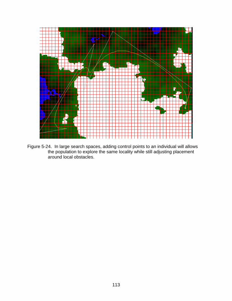
113
Figure 5-24. In large search spaces, adding control points to an individual will allows
the population to explore the same locality while still adjusting placement around local obstacles.
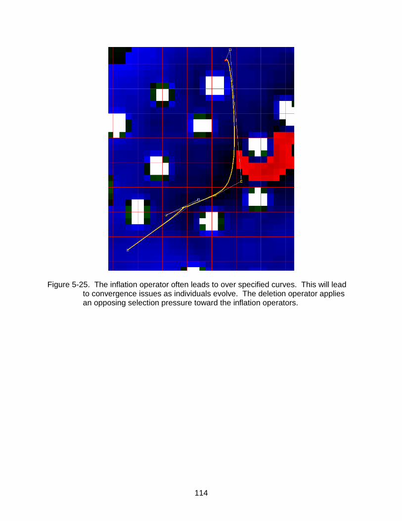
114
Figure 5-25. The inflation operator often leads to over specified curves. This will lead
to convergence issues as individuals evolve. The deletion operator applies an opposing selection pressure toward the inflation operators.

115
Figure 5-26. The deletion operator will also remove points that clump together which
have a negligible effect on the over path cost but will hinder convergence during dynamic adjustment.

116
Figure 5-27. Equal crossover of the blue and orange genomes leads to the resultant
red offspring genome.
Figure 5-28. The effect of the blocking operator on a spline.

117
A
B Figure 5-29. The result of the Fan operation of a spline. A) The spline with a control
point added during the Fan operation. B) The original spline the Fan procedure labeled with green arrows.
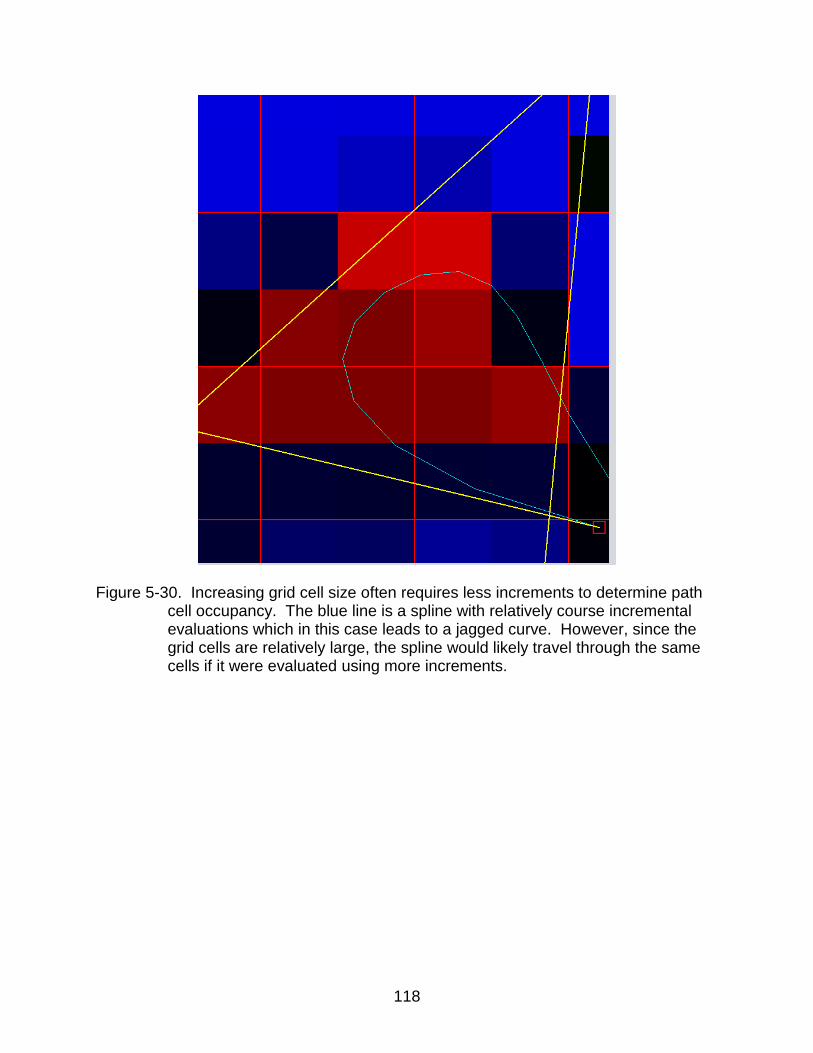
118
Figure 5-30. Increasing grid cell size often requires less increments to determine path
cell occupancy. The blue line is a spline with relatively course incremental evaluations which in this case leads to a jagged curve. However, since the grid cells are relatively large, the spline would likely travel through the same cells if it were evaluated using more increments.

119
Figure 5-31. A high resolution grid needs more control points to accurately approximate
a minimum cost path.

120
Figure 5-32. Low resolution populations need less control points to define candidate
solutions because splines with more control points will likely evaluate to the same cost as those with fewer control points.
Figure 5-33. Building blocks combined in an unstructured gene pool to create
individuals which are then evolved in populations with combination and selection pressure.

121
Figure 5-34. Downscaling a population produces search spaces with grid cells are
varying size. The bottom right grid shows the original traversability data resolution while the upper left grid shows the highest downscaling search space.
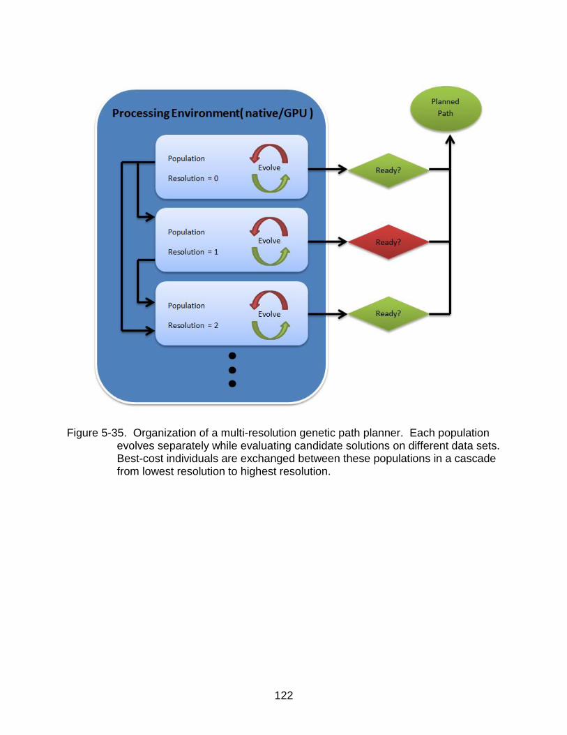
122
Figure 5-35. Organization of a multi-resolution genetic path planner. Each population
evolves separately while evaluating candidate solutions on different data sets. Best-cost individuals are exchanged between these populations in a cascade from lowest resolution to highest resolution.

123
CHAPTER 6
EXPERIMENTAL RESULTS
Setup
The original goal of this research was to create a planner and run it in a real world
setting using a low level, deterministic reactive controller to arbitrate localized sensor
readings while using the genetic planner as a high level reactive guide. For these
expected conditions, the CIMAR Urban Navigator autonomous vehicle was used to
gather sensor data from various LIDAR units positioned on the vehicle. However, after
some data was collected, it was clear that the abstracted traversability values did not
produce enough comprehensive terrain data to merit clear path planning over the
search spaces defined in this research. Also, as only roads were able to be driven on
using the specific platform, the data tended to be corridors of roads which is not
generally well suited for the planner as it was designed and can be better navigated
using a deterministic planner after abstracting the information to roads or road corridors
(Figure 6-1 and Figure 6-2).
Considerable effort would have been needed to create the rich search spaces this
research is aimed at addressing so a simulated environment was instead used to
implement and test the ideas contained in this research. To create realistic landscapes,
the L3DTPro videogame level designer was used. The program can generate any
desired height map size and contains an easy to use editor which was leveraged for this
research to create specific testing scenarios. Both small (Figure 6-3) and large (Figure
6-4) grids were generated with this program and altered when needed to conform to
each testing simulation. Dynamic objects were inserted into this environment using
masking maps when cell costs were being calculated (Figure 6-5). Also, sensor noise
124
was simulated by applying various levels of Gaussian noise to these masks (Figure 6-
6). In this way, relatively realistic, very large search spaces were generated and tested
without the need for real sensor data. The implementation can still work without a
complete set of data by applying the threshold mask to the data which highly guides the
search away from these areas (Figure 6-7).
Testing was set up to try to record some quantitative measure of how well the
reference implementation functions under various conditions. Genetic algorithm
methods are usually compared by the ability of the population to converge to a semi-
optimal solution. This criterion is appropriate for our testing if the evaluation time for the
convergence is also taken into account. Individual population evaluation is important
but a better measure of the system is how fast the unscaled, highest resolution, search
space can produce a solution and how the fitness of this solution converges. Simply
evaluating the highest-resolution population alone is not reasonable because of the
seeding exchanges that are done between the resolutions. The overall solution may
actually be generated by running the highest resolution population at a slower rate and
the lower resolution populations at a higher rate. Thus, the availability of a solution at
any given resolution is also taken into account when judging the success or failure of
the process.
Random Bias
Evolutionary Computation in inherently random by definition and results
sometimes displayed wide variations when testing under the same conditions. This
assorted convergence was traced back to how each population is initialized to different
random sets of individuals. When the same initial population was reused over separate
trials, the convergence paths tended to be similar (Figure 6-8). However, aberrations

125
did still exist when multiple cost valleys were provided in the search space and outliers
remained in some cases. This is to be expected when considering each run will
produce different random numbers while generating new individuals. The non-
convergent effects tended to be more pronounced when the population was randomized
before each test run (Figure 6-9). This leads to difficulty in assigning a testing method
which will definitively determine what methods are appropriate for inclusion into the
proposed search method. With this in mind, testing was completed by specifically
constraining some of the search spaces to valley areas where the solutions should
definitely converge to the same test valley (Figure 6-10). These tests were used to
gauge how well the populations converged on average when using the same initial
conditions across all tests. This tended to remove the random bias and seemed to
imply when the tests were successful or unsuccessful.
Testing Hardware
The hardware used for this testing consists of a NVIDIA GeForce 8800GT with
112 cores operating at 600MHz which allows for a theoretical 504GFLOPS (normal
usage rated at 330GFLOPS). Up to 512MB of global memory is available on the GPU
operating with a bandwidth of 57GB/s. This represents a low to mid-level computation
capability in terms of what is currently available when considering a price vs
performance ratio. As of April 2012, a state of the art GPU offers several hundred, if not
1000s, of cores and is able to achieve several teraFLOPS. Search space size also was
the limited by the OpenCL driver for the NVIDIA GeForce 8800GT with a maximum
buffer size of 137MB. The 8800GT was also limited to only single precision calculations
which was found not to affect the problem scope in experiments. For native CPU
calculations, an Intel Core2 Quad Q6600 was used along with 4GB of system memory

126
and a SATA2 SSD to decrease any latency involved with disk caching. The
programming environment used was Sun Java JDK1.7 but had to be changed to the 64-
bit version to allow for larger search spaces.
Static Convergence
The proposed methods were first tested using a static search space. This means
data was loaded into the hashed grid cells once, before the evolutionary process
started, and left unmodified throughout the experiment. Appropriate start and end
locations were chosen to demonstrate and test seemingly difficult convergence
situations. The static tests were divided into experiments run on relatively small areas
(1024x1024 grid cells) and those that were run on relatively large areas (8192x8192
grid cells). These sizes were chosen so that the program could store all traversability
data in available memory while still operating under the cap placed on JAVA heap sizes.
Since a 64-bit JAVA virtual machine was used, larger grid sizes could be deployed but
the practical limits of reactivity were reached on available hardware before running out
of memory. The physical representation of these cells could be anything that a user
chooses. In the CIMAR lab, these cells were ½ meter by ½ meter consolidations of
sensor information which was appropriate for the size of the vehicles. With this
analogy, the grids correspond to square areas of 512 meters (0.32 miles) in the small
case and 4096 meters (2.55 miles) in the large case.
Small Search Space
To simulate a small valley search space, a 1024x1024 grid was generated which
contained a single valley in which the solutions should converge (Figure 6-3). Different
locations within the search area were chosen and simulation trial runs were completed
to gauge how well the search can fit the environment.

127
Valley search
The first test located the start and end points of the desired path in the upper left
corner valley and lower right corner valley. After 10 trials, the solutions were almost
always able to find some path that followed the valley from start point to end point.
However, as seen in Figure 6-11, the original low cost approximation took about 3-4
seconds to converge to within 20% of the final solution after which perturbation most
likely incrementally lowered the solution to a final minimum value. The general
inclination in these results shows an exponential decreasing trend with large cost
decreases during the first part of the evolutionary process with decreasing smaller
changes as the solution converges to an asymptotic minimum. There are of course
outliers given that it is a random process. However, most trials generally converged or
are converging to the minimum valley after 20 seconds and all are expected to
converge to the same minimum eventually given that the evolutionary methods
employed are probabilistically complete.
Another test was then run with the addition of using four seeded population
threads with the same starting and ending points. This was done to allow each thread
to run on one of the available hardware cores. Figure 6-12 shows that the solution
converges to within about 20% of the final solution after only 0.5-1.0 seconds with more
populations reaching the lower bound solution. The asymptotic leveling is not at all as
pronounced as in the one population method. This is likely due to the ability for the
seeded approximations to reach the highest resolution population before this decline
occurs in the local population. The highest resolution population ran between 8-20Hz
while the other populations ran between 30-80Hz. The variance in these rates can be
attributed to the different times taken to evaluate different solutions and the adjustment

128
of solutions needed to produce the final generations. However, the overall goal of this
research is to produce the best paths in the shortest amount of time. Using the four-
threaded seeding method achieves both of these goals when compared to the single
resolution, single population method. It will not matter if the population can run at a
higher rate if better solutions can be gathered from a slower running population in a
quicker time-step.
These tests were repeated for another set of start and end points with comparable
results (Figure 6-3). However, for this test the set of points represents a situation where
multiple local minima exist and the solution process needs to find the best one. The
solution needs to explore a portion of the search space which a first may produce paths
with higher cost. Figure 6-13 shows that approximately the same time period is needed
for an asymptotic convergence for a single population. Figure 6-14 shows the benefits
of both better overall cost convergence and the time it takes to get there when using the
four-thread seeding method.
Constrained valley search
Next, the reference implementation was tested within a search space which was
created to simulate maze-finding (Figure 6-15). Peaks around a local valley were
assigned a high cost which exponentially increased the cost of any candidate solutions
that intersected these peaks. A search grid of 4096x4096 cells was used as the
environment for this test. Since the cost of a path hitting a threshold cell exponentially
increases the cost of the path, all results were graphed logarithmically to show when the
transition from obstructed to non-obstructed areas actually takes place. The
incremental improvement of the solutions cannot be seen on this graph but corresponds
to the results from the previous testing situations.

129
Figure 6-16 shows that while a single evolving population can find this minimum
valley, it happens sparingly and after some time. Only 4 of the trials resulted in finding
the solution and most take more than 12 seconds to converge. Using the 4 thread
seeding method produces better results. Seven of the 12 trials find the solution but most
of the solutions are found after 5 seconds (Figure 6-17). Simply using all 7 population
threads achieved the best results with 9 of 10 trials finding the valley (Figure 6-18).
Also, 5 of the 9 discoveries were made in less than 2.5 seconds which represents a
radical departure from the previous tests. The reason why more populations running at
a slower rate works better for this testing situation is because more of the search space
is effectively explored when more populations are running. Thus, it is more likely that
one of the random guesses will produce a viable candidate that will then be distributed
among the populations.
Static obstacle search
Next, a test 4096x4096 cell grid was created to simulate the behavior of the
reference implementation within a series of peaks. These peaks amounted to obstacles
around which the solution would need to evolve while still moving through the lower cost
valleys. The desired minimum converged solution is shown in Figure 6-19.
Running a single population produced results similar to those seen in the other
valley search tests. Figure 6-20 shows that most of the solutions converge to their
approximate final 10% range within 2.5 seconds. However, a relatively large 0.5
seconds still passes before most of the paths start to converge away from the obstacles
and find paths between the peaks. The results of using the 4 thread seeding method
are shown in Figure 6-21 and display the ability of this strategy to force convergence of
almost all the trials within 10% of their asymptotic limit under 0.5 seconds In this

130
instance, using the extra populations, one for each divisional resolution, actually
hindered the results (Figure 6-22). The 7 threaded seeding was able to generate similar
enveloped convergence as the 4 threaded seeding but usually took nearly 0.75 seconds
to accomplish. The reason for this is most likely due to the inefficiency of running more
than one population thread on the same processing core. If the amount of cores
matched the number of populations, using the 7 thread method would likely produce
comparable results to the 4 thread method
Large Search Space
Similar to the small grid tests, a Large Valley Search and Large Obstacle Search
will be evaluated in relation to both convergence quality and speed. Several 8192x8192
grids of traversability values were generated using the L3DTPro level editor software to
simulate realistic search spaces.
Valley search
A valley area was set up to test how the proposed method behaves in large search
spaces (Figure 6-23). A small threshold value was used to allow for more exploration of
each valley. The first evolutionary test was done using a single thread population
running at the highest resolution. The population was able to eventually converge in a
reasonably consistent manner (Figure 6-24). However, it took about 1-2 seconds for
the population to coalescence to the same general solution. The 4-thread multi-
resolution method was able to decrease this time to about 1 second while also reaching
the convergence limit much faster on average (Figure 6-25). Only a localized portion of
the graph is shown to emphasize the convergence of the population and not the
precipitous drop seen at the beginning of the evolutionary process. Since large initial

131
costs could, although unlikely, be caused by a solution traversing a no-go region, only
convergence was compared.
Large datasets can be quickly processed when the calculations are independent
from each other. Computation with a GPU achieves great performance gains because
so many operations can be completed at the same time. Using OpenCL, reaction and
convergence times for large dataset populations were lowered. Using a single
population with parallel OpenCL processing, generational evaluation rates of up to 30Hz
were achieved allowing convergence to start in about 1 second (Figure 6-26). However,
reaching the final convergence asymptote took about the same total time as the single
population native processing method. Better results were obtained by using the 4
thread multi-resolution method while using OpenCL (Figure 6-27). Much lower cost
solutions were available at around 40Hz with better overall asymptotic cost. Availability
in this case refers to the fact that the lowest resolution population generates fairly good
estimates in a short amount of time. However, the highest resolution population still ran
at around 15Hz using this method. Exact availability and population update rate varied
due to candidate solution path length differences as well as thread scheduling
considerations.
To attempt improvement in overall trial asymptotic agreement, tests were
completed with larger population sizes. The effect of using more candidate solutions in
a generation tends to be a greater overall exploration of the search space at the
expensive of more processing time. Experimental trials were first realized using the
native processing 4 thread multi-resolution method (Figure 6-28). The population took
almost 10 seconds to find the same relative limit as with the 100 individual trials. Using

132
a single population with native processing showed better reaction of about 5 seconds
(Figure 6-29). However, the 4 thread OpenCL method was able to keep up with the
increased calculations needed for more generational individuals and was able to
achieve a small band of asymptotic convergence when compared to the 100 individual
trials (Figure 6-30. This of course comes at a cost of reactivity with average availability
of 15Hz.
Static obstacle search
Tests were repeated on a large area with simulated static obstacles by creating a
series of peaks within a relatively flat plane (Figure 6-31). The proposed method was
first tested using native processing to find a possible solution from a start point to a goal
point which traverses the entire grid (Figure 6-32). A single population run at the
highest resolution was able to generally find asymptotic convergence within about 6
seconds (Figure 6-33) with availability limited to around 3Hz. This limit was reached in
only about 2 seconds when using the 4 thread multi-resolution method (Figure 6-34).
Availability of using the native calculations with this approach was around 60Hz.
By pushing calculations to the OpenCL kernels, dramatic increases in planning
speed were observed. The single population strategy was able to evaluate generations
at about 30 Hz but convergence suffered with asymptotic limits after about 3 seconds
(Figure 6-35). Approximate path costs were decreased by about 10% over the trials by
using the 4 thread multi-resolution method with OpenCL processing (Figure 6-36). As
before, these more similar, better cost paths ran at about 30-60Hz availability with the
highest resolution population running at around 20Hz. It is important to note that the
costs of the natively calculated individuals could not be directly compared to the
individuals calculated with OpenCL due to the differing allowances offered in each

133
circumstance. Specifically, it was found that the built in exponentiation function that
OpenCL provides takes almost 5 times longer than an approximation of the value. To
duplicate the stratification effect which makes total path costs exponentially increase
with linear increases in cell cost, each occupied cell cost was simply squared.
Dynamic Convergence
Autonomous robots generally need to function in dynamic environments. For this
reason, dynamic objects were inserted into the search space to observe any changes to
how the populations evolve and subsequently determine what modification to the
process needed to be put in place to allow for fast convergence in a dynamic
landscape. Dynamic objects were simulated by creating a value-lookup mask which is
evaluated at the same time cell occupancy is evaluated. In effect, whenever a
candidate solution was found to intersect an object, the cost of the solution was
arbitrarily raised to some large value. This would likely remove that individual from any
future generations. The object locations could then be moved by starting a different
processing thread and changing the locations and directions of movement based off a
timed sequence. This allowed for random or defined movement at specified portions
within the search space or throughout the whole search area.
The sensors used on the CIMAR vehicles tend to have two sources of noise: drift
and oscillatory noise. Drift compensation is out of the scope of this research but GA is
well suited for oscillatory data since individuals in a population or portions of the
planned path may continue throughout the generational gaps even when their solutions
are suboptimal. Gaussian noise was instead generated at various levels and injected at
a specified timed interval into the search space. The effect of this noise on

134
convergence could then be documented and any oscillatory behavior was cataloged.
However, the Gaussian noise had little if any effect on the paths which were generated.
Random Object Insertion
Random object insertion consists of allowing objects of specific sizes to be
inserted at random locations within the search space. These objects are then given
simulated movement by projecting a random trajectory for some amount of time. The
movement is then changed at some specified interval randomly so that seemingly
unpredictable movement is simulated. This test serves to display how the
implementation can function in very unpredictable environments.
The random object insertion test was first evaluated in a small search space of
1024x1024 traversability cells (Figure 6-37). Ten Random objects were inserted into
this space and a single trial was run to determine how well a single population can
adjust to many objects interrupting different portions of the desired path. Figure 6-38
shows that a single population can always find some unobstructed path through the
area and converges to the approximate minimum range within a few generations of the
disturbance. However, in many cases a minimum could not be converged upon most
likely because of another interruption at that minimum by the movement of other
objects.
Another test was run to determine if the seeding method at different resolutions
would help the convergence speed in this testing situation. The four thread method
discussed earlier was engaged and results were collected for the best fit individual in
the highest resolution population over a period of 60 seconds. No averaging of trials
was compared as the movements of the random objects would not be identical and
wouldn’t allow for an accurate appraisal of the method. Figure 6-39 shows that in

135
general, the 4 threaded, seeding approach is able to keep both a lower converged value
as well as adjust to the converged value faster than the non-seeding evolution.
Oscillatory Object Simulation
Since dynamic objects sometimes behave in an oscillatory manner, through both
sensor aberrations and actual observed behavior, the proposed planning methods were
also evaluated using a simulated object moving in a repeated motion across a defined
valley path. The object path was placed specifically to interrupt the valley in which the
solution is expected to occur (Figure 6-40 and Figure 6-41). To replicate the time at
which the converged candidate solution will be interrupted in the evolutionary process,
the dynamic obstacle was restarted for each trail at the same location and with the
same velocity.
Figure 6-42 shows that even a single population is able to adjust well to the
dynamic obstacle. There are of course deviations over trials due to the randomness
involved in the evolutionary process but the general trend is for the best-cost solution to
return to an approximate convergence in about 1 second after the interrupted valley is
cleared. As in previous tests, even when starting from the same original population,
using a single population will generally have solutions that converge to different local
minima. However, when using the four threaded seeding method, the solution is able to
quickly converge in almost all trials to the same, low cost solution over almost every test
run (Figure 6-43).
Deterministic Search Comparison
To catalog how this method is able to work in search spaces which are too large
for other deterministic methods, two A* search algorithms were tested within the same
search spaces and compared to the parallel-genetic method. The first A* used a

136
fanning approach which generally allowed for movement based on turning radius and
offset. The second A* planned using monotonic, holonomic criteria which operated
specifically on grid cell indices. While various other deterministic and nondeterministic
algorithms exist for path planning, this comparison serves as a cursory demonstration
that many searching methods may run into heavy computational burdens when
expanding the search space size. Admittedly, several unrealized optimization
techniques could have been implemented to mitigate some of the issues observed but
the overall results still serve to demonstrate how the A* methods are not appropriate for
large search spaces especially when reactive planning is required.
Both time and memory consumption were taken as metrics for comparing the A*
methods to the nondeterministic approach suggested in this research. As expected, it
was found that unconstrained expansions unreasonable amounts of time for even the
small search spaces that were tested (Figure 6-44). It was also noted that using these
methods caused considerable delay even when the allotted memory was not filled and a
solution was found. Various techniques do exist which can alleviate some of these
problems but the underlying conditions for expansive dimensionality still exist.
The first method employed to test A* was an unrestricted fanning operation which
is based on a desired minimum turning radius for the platform. It was implemented by
projecting 1 point directly along the path from the previous point and another 2 points on
each side of the projection (Figure 6-45). The costs of the expansion nodes were then
evaluated by finding the real cost of the segment intersections along with the predicted
cost of the node which was taken as the line distance from the node to the goal point.
The method turned out to be very sensitive to the specified offset distance as well as

137
the angle at which the points are projected each node. The method worked well when
these values were tuned for specific planning objectives but the search tree tended to
explode when applied to random testing instances (Figure 6-44).
The other method used to test the applicability of using A* in large search spaces
was a purely index-based strategy. This approach used the grid cells as the basis for
each node expansion (Figure 6-46). For each expansion, new nodes were tested so
that previously closed nodes did not get expanded multiple times. This only allows for
monotonic movement but for many cases the assumption is appropriate. The method
was able to find an optimal path both in a reasonable amount of time and also for more
test cases. However, the search still suffered greatly as the search space size
increased. It took several seconds for solutions to be found for path length of several
hundred cells with practical applicability limited to the 1024x1024 test space. Of course,
better performance could be gained by adopting strategies noted throughout the
literature but the problem remains that the deterministic method does not function well
in large search spaces when reactive plans need to be generated.

138
Figure 6-1. Sample test run of data gathered from the CIMAR UrbanNavigator LIDAR
sensors.

139
Figure 6-2. Map describing the path taken for gathering the data in Figure 6-1

140
Figure 6-3. A small valley search grid of 1024x1024 cells. Red cells represent low
costs, blue medium cost, and green high costs. Within each color, dark tints are lower cost than lighter shades. The thick yellow line represents the approximate least cost spline path. The yellow boxes display the control points which define the spline. The thin grey line shows the control point order.

141
Figure 6-4. A large search grid of 8192x8192 cells. White cells represent no-go regions
within the search space.

142
Figure 6-5. A moving intersecting a candidate solution. The object is defined by a
square no-go region at a defined point within the space.

143
Figure 6-6. An exaggerated Gaussian noise mask applied to a small search space.

144
Figure 6-7. A threshold mask applied to the search grid to focus the search within a
desired area.
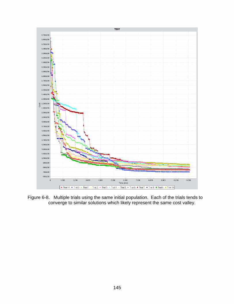
145
Figure 6-8. Multiple trials using the same initial population. Each of the trials tends to
converge to similar solutions which likely represent the same cost valley.

146
Figure 6-9. Trials with multiple cost valley options when a population is seeded
randomly before each trial.

147
Figure 6-10. Constrained valley maze test with the desired solution labeled in green.

148
Figure 6-11. Small valley search convergence over 10 trials using single threaded
population running under the highest resolution of 1024x1024.

149
Figure 6-12. Small valley search convergence over 12 trials using 4-thread multi-
resolution approach. The displayed costs are for the population running under the highest resolution of 1024x1024.

150
Figure 6-13. Another setup of the small valley search convergence over 10 trials using
single threaded population running under the highest resolution of 1024x1024.

151
Figure 6-14. Another setup of the small valley search convergence over 12 trials using
4-thread multi-resolution approach. The displayed costs are for the population running under the highest resolution of 1024x1024.

152
Figure 6-15. Desired converged solution for the constrained valley search test.
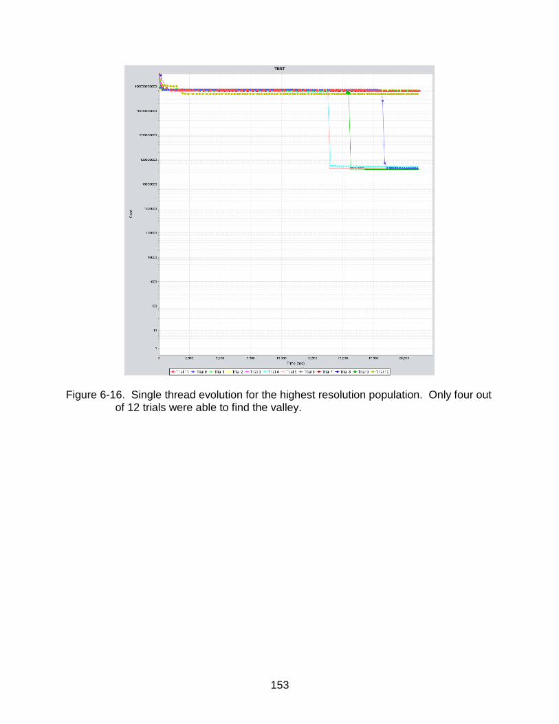
153
Figure 6-16. Single thread evolution for the highest resolution population. Only four out
of 12 trials were able to find the valley.

154
Figure 6-17. 12 trials of the four thread multi-resolution strategy to find the solution in
the constrained valley search. Seven of the 12 trials were able to find the valley but more than half took longer than 7 seconds.

155
Figure 6-18. Constrained valley search using a population at each resolution.

156
Figure 6-19. The desired minimum cost path for the small search space static obstacle
tests.

157
Figure 6-20. Single population at highest 4096x4096 resolution for the small search
space static obstacle converge test with 10 trials.

158
Figure 6-21. Static obstacle small search space test using the four thread multi-
resolution method with 12 trials.

159
Figure 6-22. Small search space static obstacle test results for the 7 population multi-
resolution approach.

160
Figure 6-23. A 8192x8192 search grid describing a series of valleys. The yellow line
shows the desired convergence path.

161
Figure 6-24. Trial runs on the highest resolution grid using native calculation with no
seeding on the large valley sample.

162
Figure 6-25. Trials run with the 4 thread multi-resolution method using native
calculation on the large valley sample.
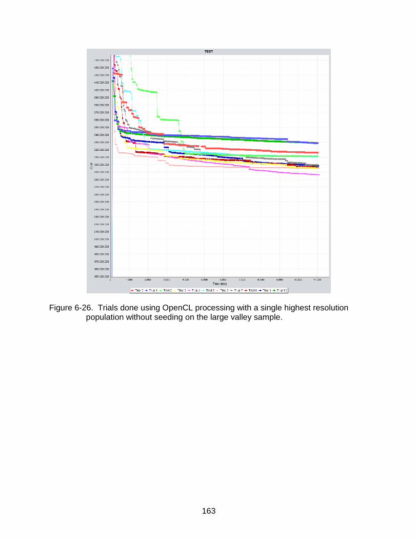
163
Figure 6-26. Trials done using OpenCL processing with a single highest resolution
population without seeding on the large valley sample.
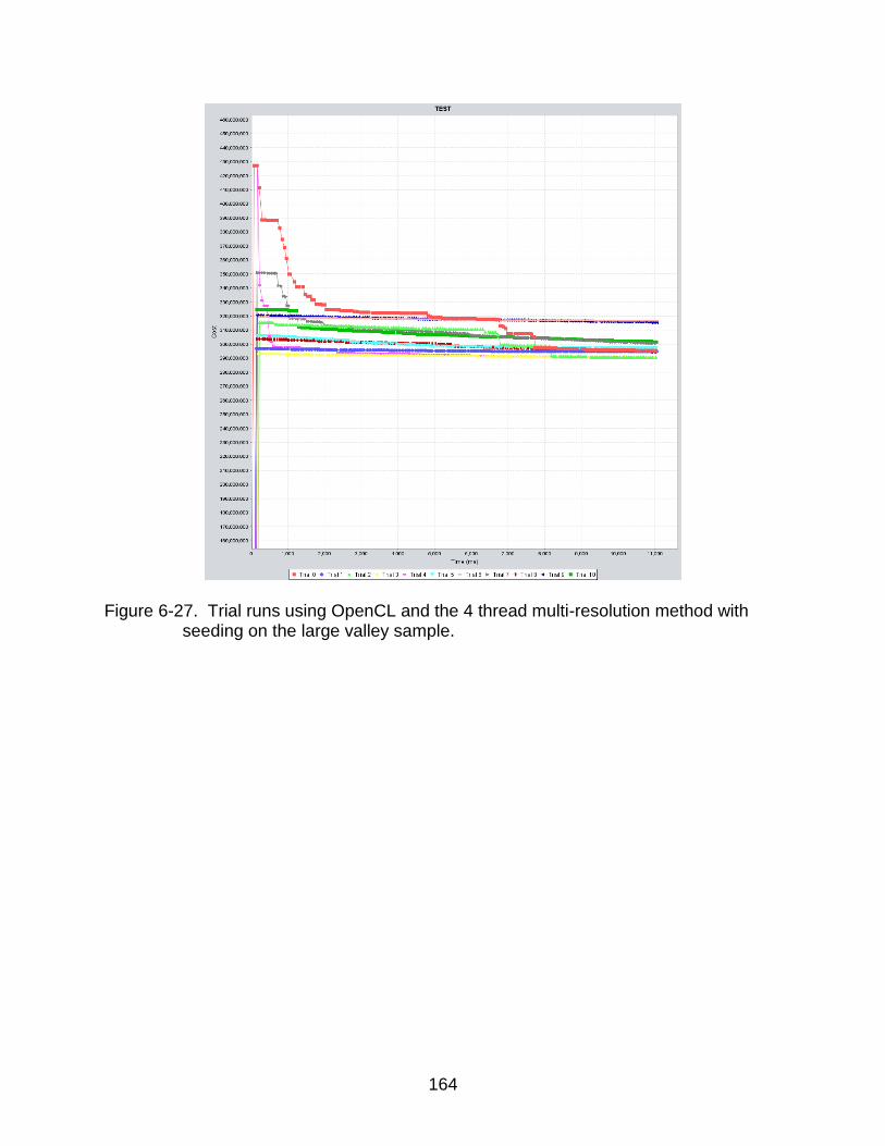
164
Figure 6-27. Trial runs using OpenCL and the 4 thread multi-resolution method with
seeding on the large valley sample.

165
Figure 6-28. Trial runs using native processing with the 4 thread multi-resolution
method while maintaining 300 individuals on the large valley sample.

166
Figure 6-29. Trial runs using native processing with a single high resolution population
while maintaining 300 individuals on the large valley sample.

167
Figure 6-30. Trial runs using OpenCL processing with the 4 thread multi-resolution
method while maintaining 300 individuals on the large valley sample.

168
Figure 6-31. A 3-D view of large static obstacle search space with peaks.
Figure 6-32. A desired path across the large static obstacle sample space. The thin
yellow line represents a lost cost prediction through the area.

169
Figure 6-33. Trials run using native calculation with a single high-resolution population
in the large static obstacle sample.

170
Figure 6-34. Trials using the 4 thread multi-resolution seeding method with native
calculations in the large static obstacle search space.

171
Figure 6-35. Trial runs using OpenCL processing with a single high resolution
population in the large static obstacle search space.

172
Figure 6-36. Trial runs using OpenCL processing with the 4 thread multi-resolution
method in the large static obstacle sample.

173
A
B Figure 6-37. Random moving object insertion. A) Path adjustment to compensate for
moving objects. B) Path convergence back to minimum valley after objects have moved to other areas within the search space.

174
Figure 6-38. Convergence costs of single population resolution running at the
1024x1024 resolution for the random moving object insertion test. Each spike in the graph represents the adjustment made in the path when a moving object intersects the converged solution.

175
Figure 6-39. A comparison between the single population evolutionary method (blue)
and the 4 thread multi-resolution method (red) for the 1024x1024 resolution under the random moving object insertion test. The parallel multi-resolution method is able to generally keep a lower path cost and adjust to interruptions in less time than the single population strategy.

176
Figure 6-40. Desired path valley for the oscillatory object test. Before the moving
object intersects the path, the solution converges to the valley within the search grid.
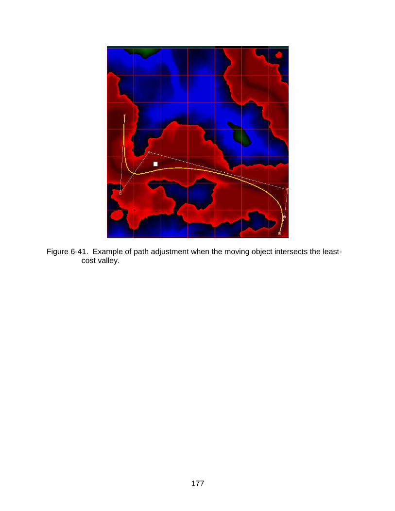
177
Figure 6-41. Example of path adjustment when the moving object intersects the least-
cost valley.

178
Figure 6-42. Single population adjustment running at the 1024x1024 resolution for the
oscillatory object test. Each bump in the graph represents the adjustment made after a moving object interrupted the converged solution path.

179
Figure 6-43. Convergence for the oscillatory object test when running the 4 thread
multi-resolution method. Each bump in the graph occurs when the moving object obstructs the converged solution.

180
Figure 6-44. Unconstrained expansion allowing for non-monotonic movement within the sample search space. Each yellow segment represents the open node and its parent node to show the expansion direction.

181
Figure 6-45. Node expansion for unconstrained A* searching.
Figure 6-46. Indexed A* expansion within a small sample search space.

182
CHAPTER 7
DISCUSSION AND FUTURE WORK
Assessment of Fitness to Problem Scope
This research is admittedly designed for a problem that is not widely occurring in
the field of autonomous robotics. However, its applicability to future platforms can only
be called into question if one discounts the overall trends observed in the field over the
past few years. Increasing data loads are provided by more accurate sensors at higher
update rates and resolutions. However, one of the main driving forces behind
autonomous robotics is to create reactivity in a human-appropriate timeframe. This
research addresses both of these issues as applied to the specific problem of path
planning. The results displayed in this research prove that these, or similar, methods
can be used to mitigate the problems discussed above while at the same time
producing autonomous robotic platforms able to meet ever increasing operating
constraints.
Future Work
One of the main reasons outlined in the discussion for using evolutionary
computation over deterministic methods is the ability to deal with expansive search
spaces. This work has focused on the expansion of a two dimensional workspace by
adding more 2-D data. Often, multi-objective problems or platforms with many degrees
of freedom will also increase the size of the search space. One future topic to consider
which is beyond the scope of the current work is how to adapt the proposed method to
these different instances. A question remains as to whether the scaling seen with a 2-D
search area will also be observed to converge in many dimensions.

183
Another course of possible study is applying these techniques to other forms of
classification or optimization which may be hindered by increasing data spaces. This
method is a novel approach to exploring such fields and may be applicable to entirely
different representations or time constraints. One necessary property of a prospective
problem domain is the ability of a dataset to be discretized at different resolutions or at
simplified representations. Care must be taken when deciding if the cost of down
sampling data is less than the computational or time costs in abstracting the data set
into to some other, more appropriate structured dataset. Most planning problems
involve search spaces that can be sampled as described in this work and would likely
benefit from this strategy.
While a GPU was used for parallelization in this research, other methods exist for
parallel calculation which may yield better results. A GPU was chosen in this instance
simply because of its low cost and high performance but other methods such as cloud
computing, where jobs are loaded to abstracted and expandable computing resources,
could also have been used if communication latency issues were arbitrated. Other
methods such as clustered computer nodes or even the Cell processors prevalent in the
PlayStation 3 game consoles could also be levered in the same manner as the GPU.
Due to the highly formalized evaluation methods, hardware could also be specifically
designed to calculate individual fitness on units like FPGAs or CPLDs. These methods
would allow for a more robust planner in that generational evaluation could be run
faster, and converge faster, while maintaining more accurate path evaluations with
double point precision.
184
Another possible extension of this work could be in how to apply the parallel
seeding methodologies to different basic planning algorithms. In this research, a
Genetic Algorithm was used to evaluate the solutions but almost any method that can
be seeded with solutions could also be used in place of the Genetic Algorithm. Even
though extremely good performance was found throughout the specific test cases
evaluated in this research, many areas of application may not be appropriate for
application of a Genetic Algorithm. This would include direct motion control of robotic
platforms or some other direct interaction with the physical world. The unpredictability
of the genetic algorithm is not appropriate for instances where human life or expensive
machinery is in question. More predictable methods can be used for these instances
but may still benefit from the parallel seeding process.
In this research, populations were defined by equally consolidating the simulated
sensor resolution until a lower limit is reached. In future investigations, other strategies
could be developed that may produce comparable results with differing amounts of
populations. This research did not attempt to classify or constrain when and how
seeded candidate solutions moved between populations. Other strategies could be
explored such as lowering the execution rates at which low-producing populations run
while increasing evaluation rates of populations which produce better individuals. One
could also use less total populations if faster overall convergence is desired for the
specific problem domain. These extensions would allow for possibly better efficiency
when computational resources are limited or power constrains on a platform make
varied execution times more relevant.

185
The initial work in this research focused on an unconstrained search space with
obstacles represented as vectorized abstractions of shapes. The research then went
into using normalized discretizations of traversability cells. The former approach takes
much less storage space and is appropriate for certain platform configurations. Future
work could be done in applying the spline methods discussed in this paper to a vector
search space. Efficient spatial storage of the vector object would need to be completed
so that the spline evaluations need not test each obstacle in the entire search space.
Similar strategies were noted in the literature but will most likely benefit from the
additional parallel anytime method developed in this research.
Conclusions
It is generally accepted that the amount of information an autonomous platform will
need to process, from both sensors and external sources, will increase exponentially in
the coming years. This research offers a novel approach in which performance of a
global path planner can be maintained in very large search spaces. The proposed
method used a unique mix of spline representation building blocks to evolve a path in
which a holonomic robot can traverse. Domain specific combinatorial and mutation
operations were needed to optimize path formation and fitness evaluation. Adapting a
GA to generate paths in dynamics environments is important since autonomous robots
rarely operate in static environments.
The second major contribution on this work is a path planner that is able to
generate a viable plan in any given time-step. The only projected limiting factor is the
time it takes for one individual to be evaluated at a given resolution. Preservation of
reactivity is important for an autonomous platform especially when considering one

186
moving at high speeds. The implementation of a novel tiered GA allows a path to be
generated at different time-steps independent of the desired speed of the vehicle.
While only a 2-D planning method was considered in, probabilistically complete
planners are seen as the only viable way in which to circumvent the exponential rise in
search space size as configuration dimensionality increases linearly. Future
autonomous robots will likely need many more degrees of freedom to appropriately
traverse a 3-D non-structured environment. The ideas formulated and tested in this
work will serve as a basis on which future path planners can build on to mitigate the
deleterious effects of adding many degrees of freedom to a robotic system.

187
APPENDIX A EXAMPLE SPLINE CALCULATION
An example of how the parametric spline is calculated will be shown. A 3rd order
B-Spline with 5 control points will be evaluated with equal knot spacing and clamped
start and end points. The number of divisions for this category of spline is difference of
control point count and spline degree. Thus, with 5 control points, there will be two
divisions spanning the curve. The first of these divisions will be calculated by first
finding the raw divisional 4x4 matrix, conditioning that matrix with the specified control
points and finally evaluating the conditioned vector with 50 increments from 0 to 0.5.
The first step in the process is to calculate the raw divisional 4x4 matrix using the De
Boor Algorithm.
Figure A-1. De Boor process for parametric evaluations
With 5 control points, 3rd degree and clamped conditions, there will be 9 knot
points placed along the curve. Also, by using equally spaced knots, there will be two
incremental division ranges.

188
0 0.5 1.0
Figure A-2. Division separation for example spline with 5 control points
The most important aspect of the De Boor algorithm is that the intermediate N
variables will only evaluate to non-zero values when t is within the divisional incremental
range. All other intermediate N variables will not contribute to the final solution. In this
case, the calculations will be done in the first division so the knot and knot range
will be used resulting in a non-zero value of . Using this idea, all the needed
recursive evaluations can be described with the following graph of relations.
Figure A-3. Pyramid structure of N value dependencies.
Working from the base relation, the following calculations can be completed
keeping the parameterized t value encoded for later evaluation. The goal of these
calculations will be a so called raw 4x4 matrix of numbers that will then be combined
with the divisional control points to condition the matrix.

189
(1)
(2)
(3)
(4)
(5)
(6)
(7)
(8)
(9)
(10)
(11)
(12)
(13)

190
(14)
(15)
(16)
(17)
(18)
(19)
(20)
(21)
(22)
(23)
(24)
(25)
(26)
(27)

191
(28)
The values that will be used in the spline summation are
(29)
(30)
(31)
(32)
Combining with the applicable local control points gives
(33)
(34)
Now, assembling in a 4x4 matrix form
(35)
Conditioning the raw matrix will be the combination of the P and 4x4 matrix while
the increment evaluations will be combining all 3 matrices. The 4x4 matrix may be
reused for each evaluation of the 1st division of any 3rd degree B-spline with 5 control
points with clamped end conditions as well as equal knot spacing. The conditioned
matrix may be reused with different t-step incremental resolutions.

192
APPENDIX B EXAMPLE TEST MOVIES
Several videos showing the reference implementation are provided to further
explain the use of the method in testing. The first example shows the use of the planner
in a small search valley test area. The path end point is moved dynamically around the
search area and the planned path follows while attempting to optimize the route in real
time.
Object B-1. Sample of the small valley test area (.avi file 5.2MB)
The next sample shows the convergence process in the constrained valley test.
First, a low resolution population is allowed to attempt convergence. Next, the 4 thread
seeding method is activated allowing seed individuals to propagate across the threads.
Seeded solutions appear red while locally evolved solutions appear yellow.
Object B-2. Sample of the constrained valley test area (.avi file 1.8MB)
A large test area is shown next with simulated static obstacles. The solution is
allowed to converge at a low resolution and then shown to converge to a different local
minimum when the 4 thread method is turned on.
Object B-3. Large static obstacle test area (.avi file 7.0MB)
Finally, an example of the dynamic obstacle testing is displayed using a low
resolution. The 4 thread method with seeding is then shown to be able to reject the
obstructions more quickly.
Object B-4. Single dynamic oscillatory object test area (.avi file 6.3MB)
193
LIST OF REFERENCES
[1] R. I. Lung and D. Dumitrescu, “A collaborative model for tracking optima in dynamic environments,” in Proc. IEEE Congress Evolutionary Computation CEC 2007, pages 564–567, 2007.
[2] Anabela Simões and Ernesto Costa, “A comparative study using genetic algorithms to deal with dynamic environments,” in EvoWorkshops 2007, Applications of Evolutionary Computing, LNCS 4448 , 2007.
[3] Anthony Stentz, “Optimal and efficient path planning for partially-known environments,” in International Conference on Robotics and Automation, pages 3310–3317, 1994.
[4] Anthony Stentz, “The focussed D* algorithm for real-time replanning,” in International Joint Conference on Artificial Intelligence, pages 1652–1659, 1995.
[5] TM Anand, “Reactive deformation of path for navigation among dynamic obstacles,” in IEEE International Conference on Robotics and Biomimetics (ROBIO), 2009, pages 544 –549, Dec. 2009.
[6] C. Hernandez, X. Sun, S. Koenig, and P. Meseguer, “Tree adaptive A*,” in International Joint Conference on Autonomous Agents and Multiagent Systems, 2011.
[7] Valérie Boor, Mark H. Overmars, and A. Frank Van Der Stappen, “The gaussian sampling strategy for probabilistic roadmap planners,” in International Conference on Robotics and Automation, pages 1018–1023, 1999.
[8] Lydia E. Kavraki and Jean Claude Latombe, “Probabilistic roadmaps for robot path planning,” in Practical Motion Planning in Robotics: Current Approaches and Future Directions, vol. 53, 1998.
[9] O. Khatib, “Real-time obstacle avoidance for manipulators and mobile robots,” in Proc.1985 IEEE International Conference on Robotics and Automation, volume 2, pages 500 – 505, Mar 1985.
[10] J. Barraquand, B. Langlois, and J.-C. Latombe, “Numerical potential field techniques for robot path planning,” in IEEE Transactions on Systems, Man, and Cybernetics, 22:224–241, 1992.
[11] Jérôme Barraquand, Lydia E. Kavraki, Jean Claude Latombe, Tsai yen Li, Rajeev Motwani, and Prabhakar Raghavan, “A random sampling scheme for path planning,” in International Journal of Robotic Research, 16:759–774, 1997.

194
[12] Prahlad Vadakkepat, Tong Heng Lee, and Liu Xin, “Application of evolutionary artificial potential field in robot soccer system,” in IFSA World Congress and 20th NAFIPS International Conference, July 2001.
[13] Jur P. Van Den Berg, Dave Ferguson, and James Kuffner, “Anytime path planning and replanning in dynamic environments,” in International Conference on Robotics and Automation, pages 2366–2371, 2006.
[14] Geofirey Hollinger, Athanasios Kehagias, Sanjiv Singh, Dave Ferguson, and Siddhartha Srinivasa, “Anytime guaranteed search using spanning trees,” The Robotics Institute, Carnegie Mellon University, Pittsburgh, PA, Tech. Rep. CMU-RI-TR-08-36, August 2008.
[15] Dave Ferguson and Anthony Stentz, “Anytime RRTS,” in International Conference on Intelligent Robots and Systems - IROS, pages 5369–5375, 2006.
[16] Maxim Likhachev, Dave Ferguson, Geoff Gordon, Anthony Stentz, and Sebastian Thrun, “Anytime search in dynamic graphs,” in Artificial Intelligence, 172:1613–1643, 2008.
[17] Javier Antich, Alberto Ortiz, and Javier Minguez, “A bug-inspired algorithm for efficient anytime path planning,” in International Conference on Intelligent Robots and Systems - IROS, pages 5407–5413, 2009.
[18] Arfath Pasha, “Geometric Bin Packing Algorithm for Arbitrary Shapes,” M.S. thesis, University of Florida, 2003.
[19] John R. Koza, Forrest H Bennett, David Andre, and Martin A. Keane, “Automated design of both the topology and sizing of analog electrical circuits using genetic programming,” in Artificial Intelligence in Design '96, pages 151-170, Dordrecht, 1996.
[20] Harish Subramanian, Subramanian Ramamoorthy, Peter Stone, and Benjamin J. Kuipers, “Designing safe, profitable automated stock trading agents using evolutionary algorithms,” in Genetic and Evolutionary Computation Conference, pages 1777–1784, 2006.
[21] Stewart W. Wilson, “Classifier fitness based on accuracy,” in Evolutionary Computation, pages 149–175, 1995.
[22] Menglin Li, Colm O’Riordan, and Seamus Hill, “An analysis of multi-chromosome GAs in deceptive problems,” in Proceedings of the 13th annual conference on Genetic and Evolutionary Computation, GECCO ’11, pages 1021–1028, New York, NY, USA, 2011.

195
[23] D. E. Goldberg, B. Korb, and K. Deb, “Messy genetic algorithms: Motivation, analysis, and first results,” in Complex Systems, No. 3., pp. 493-530, 1989.
[24] Dipankar Dasgupta and Douglas R, “Mcgregor. SGA: A structured genetic algorithm,” in Technical Report no. IKBS-11-93.ps.Z, Dept. of Computer Science, University of Strathclyde, UK, April 1993.
[25] Ben S. Hadad and Christoph F. Eick, “Supporting polyploidy in genetic algorithms using dominance vectors,” in Evolutionary Programming, pages 223–234, 1997.
[26] Cem Hocaoglu and Arthur C. Sanderson, “Planning multiple paths with evolutionary speciation,” in IEEE Transactions on Evolutionary Computation, pages 5:169–191, 2001.
[27] Shumeet Baluja, “A massively distributed parallel genetic algorithm (mdpga),” Carnegie Mellon University, Tech. Rep. CMU-CS-92-196R, 1992.
[28] Guan Wang, Degang Wu, Wenjin Chen, and Kwok Yip Szeto, “Importance of information exchange in quasi-parallel genetic algorithms,” in Proceedings of the 13th annual conference companion on Genetic and evolutionary computation, GECCO ’11, pages 127–128, New York, NY, USA, 2011.
[29] Shumeet Baluja, “Structure and performance of fine-grain parallelism in genetic search,” in International Conference on Genetic Algorithms, pages 155–162, 1993.
[30] Erick Cant, “Designing efficient and accurate parallel genetic algorithms,” in International Symposium on Physical Design, 1999.
[31] Hao Chen, Nicholas S. Flann, and Daniel W. Watson, “Parallel genetic simulated annealing: A massively parallel simd algorithm,” in IEEE Transactions on Parallel and Distributed Systems, pages 9:126–136, 1998.
[32] Pascal Comte, “Design & implementation of real-time parallel GA operators on the IBM cell processor,” in Proc. of the 11th Annual conference on Genetic and Evolutionary Computation, pages 1–8, 2009.
[33] Hirosuke Horii, Susumu Kunifuji, and Teruo Matsuzawa, “Asynchronous island parallel GA using multiform subpopulations,” in Lecture Notes in Computer Science, pages 122–129, 1999.

196
[34] H.G. Cobb and Naval Research Lab Washington DC, “An investigation into the use of hypermutation as an adaptive operator in genetic algorithms having continuous, time-dependent nonstationary environments,” Defense Technical Information Center, 1990.
[35] John J. Grefenstette, “Genetic algorithms for changing environments,” in Parallel Problem Solving from Nature, pages 139–146, 1992.
[36] F. Vavak, K. A. Jukes, and T. C. Fogarty, “Performance of a genetic algorithm with variable local search range relative to frequency of the environmental changes,” in Genetic Programming 1998: Proceedings of the Third Annual Conference, 1998.
[37] Anabela Simões and Ernesto Costa, “Using biological inspiration to deal with dynamic environments,” in Proceedings of the Seventh International Conference on Soft Computing, Brno, Czech Republic, June 2001.
[38] Shengxiang Yang, “Non-stationary problem optimization using the primal-dual genetic algorithm,” in IEEE Congress on Evolutionary Computation, 2003.
[39] Shengxiang Yang and Hendrik Richter, “Hyper-learning for population-based incremental learning in dynamic environments,” in IEEE Congress on Evolutionary Computation, pages 682–689, 2009.
[40] Hongfeng Wang, Dingwei Wang, and Shengxiang Yang, “A memetic algorithm with adaptive hill climbing strategy for dynamic optimization problems,” in Soft Computing, 13:763–780, 2009.
[41] Hendrik Richter, “Detecting change in dynamic fitness landscapes,” in IEEE Congress on Evolutionary Computation, pages 1613–1620, 2009.
[42] Gregory J. Barlow and Stephen F. Smith, “A memory enhanced evolutionary algorithm for dynamic scheduling problems,” in EvoWorkshops, pages 606–615, 2008.
[43] Maury M. Gouvea Jr. and Aluizio F. R. Araújo, “Diversity-based model reference for genetic algorithms in dynamic environment,” in IEEE Congress on Evolutionary Computation, pages 4639–4645, 2007.
[44] Hussein A. Abbass, Kumara Sastry, and David E. Goldberg, “Oiling the wheels of change: The role of adaptive automatic problem decomposition in non-stationary environments,” in Computing Research Repository, 2005.
197
[45] I. Tanev and K. Yuta, “Epigenetic programming: an approach of embedding epigenetic learning via modification of histones in genetic programming,” in The 2003 Congress on Evolutionary Computation, volume 4, pages 2580 – 2587, Dec. 2003.
[46] Juan Manuel Ahuactzin, El ghazali Talbi, Pierre Bessiere, and Emmanuel Mazer, “Using genetic algorithms for robot motion planning,” in European Conference on Artificial Intelligence, volume 708, pages 671–675, 1992.
[47] Dmitry Berenson, James Kuffner, and Howie Choset, “An optimization approach to planning for mobile manipulation,” in International Conference on Robotics and Automation, pages 1187–1192, 2008.
[48] Magdalena D. Bugajska and Alan C. Schultz, “Anytime coevolution of form and function,” in IEEE Congress on Evolutionary Computation, pages 359–366, 2003.
[49] Peter J. Bentley, “Adaptive fractal gene regulatory networks for robot control,” in Workshop on Regeneration and Learning in Developmental Systems in the Genetic and Evolutionary Computation, 2004.
[50] Carlos E. Thomaz, Marco Aurélio Cavalcanti Pacheco, and Marley B. R. Vellasco, “Mobile robot path planning using genetic algorithms,” in International Work-Conference on Artificial and Natural Neural Networks, pages 671–679, 1999.
[51] Sanjeev Kumar, “A developmental genetics-inspired approach to robot control,” in Genetic and Evolutionary Computation Conference, pages 304–309, 2005.
[52] T. Geisler and T. W. Manikas, “Autonomous robot navigation system using a novel value encoded genetic algorithm,” in Congress of Evolutionary Computation, 2002.
[53] Wang Hong-jian, Zhao Jie, Bian Xin-qian, and Shi Xiao-cheng, “An improved path planner based on adaptive genetic algorithm for autonomous underwater vehicle,” in IEEE International Conference on Mechatronics and Automation, pages 857 – 861 Vol. 2, Aug. 2005.
[54] T.P. Fries, “Autonomous robot motion planning in diverse terrain using soft computing,” in IEEE Mountain Workshop on Adaptive and Learning Systems, pages 177 –182, July 2006.
[55] Salvatore Candido, “Autonomous robot path planning using a genetic algorithm,” University of Illinois at Champaign-Urbana, 2005.

198
[56] Yanrong Hu and Simon X. Yang, “A knowledge based genetic algorithm for path planning of a mobile robot,” in International Conference on Robotics and Automation, pages 4350–4355, 2004.
[57] A. Elshamli, H.A. Abdullah, and S. Areibi, “Genetic algorithm for dynamic path planning,” in Canadian Conference on Electrical and Computer Engineering, pages 677 – 680 Vol.2, May 2004.
[58] H. Burchardt and R. Salomon, “Implementation of path planning using genetic algorithms on mobile robots,” in IEEE Congress on Evolutionary Computation, pages 1831 –1836, 2006.
[59] Gihan Nagib and W. Gharieb, “Path planning for a mobile robot using genetic algorithms,” in International Conference on Electrical, Electronic and Computer Engineering, 2004.
[60] Kamran H. se Dighi, Kaveh Ashenayi, Theodore W. Manikas, Roger L. Wainwright, and He Ng ming Tai, “Autonomous local path planning for a mobile robot using a genetic algorithm,” in IEEE Congress on Evolutionary Computation, 2004.
[61] Jie Zhao, Lei Zhu, Gangfeng Liu, Gang Liu, and Zhenfeng Han, “A modified genetic algorithm for global path planning of searching robot in mine disasters,” in International Conference on Mechatronics and Automation, pages 4936 –4940, Aug. 2009.
[62] Chi-Tsun Cheng, Kia Fallahi, Henry Leung, and Chi Kong Tse, “An AUVs path planner using genetic algorithms with a deterministic crossover operator,” in International Conference on Robotics and Automation, pages 2995–3000, 2010.
[63] Neda Shahidi, Hadi Esmaeilzadeh, Marziye Abdollahi, and Caro Lucas, “Memetic algorithm based path planning for a mobile robot,” in IJCI - IJIT - IJSP - Conferences, pages 56–59, 2004.
[64] Pu Shi and Yujie Cui, “Dynamic path planning for mobile robot based on genetic algorithm in unknown environment,” in Control and Decision Conference (CCDC), 2010 Chinese, pages 4325 –4329, May 2010.
[65] Han-Chih Chang and Jing-Sin Liu, “High-quality path planning for autonomous mobile robots with 3-splines and parallel genetic algorithms,” in 2008 IEEE International Conference on Robotics and Biomimetics, pages 1671 –1677, Feb. 2009.
[66] I.K. Nikolos, K.P. Valavanis, N.C. Tsourveloudis, and A.N. Kostaras, “Evolutionary Algorithm Based 3-D Path Planner for UAV Navigation,” in IEEE Mediterranean Conference on Control and Automation, 2001.

199
[67] I.K. Nikolos, K.P. Valavanis, N.C. Tsourveloudis, and A.N. Kostaras, “Evolutionary algorithm based offline/online path planner for UAV navigation,” in IEEE Transactions on Systems, Man, and Cybernetics, Part B: Cybernetics, 33(6):898 – 912, Dec. 2003.
[68] Shashi Mittal and Kalyanmoy Deb, “Three-dimensional offline path planning for UAVs using multiobjective evolutionary algorithms,” in IEEE Congress on Evolutionary Computation, pages 3195–3202, 2007.

200
BIOGRAPHICAL SKETCH
Drew Lucas was born and raised in Crystal Beach, Florida and graduated from the
Palm Harbor University High School International Baccalaureate Program in 2002. Mr.
Lucas received his B.S degree in Mechanical Engineering from the University of Florida
in Gainesville, Florida in 2006. He continued at the University of Florida and went on to
receive his M.S. in Mechanical Engineering in 2009. Mr. Lucas is currently working as a
Research Assistant at the Center for Intelligent Machines and Robotics (CIMAR) at the
University of Florida with a concentration on path planning and knowledge
representation and storage.


![Parallel heterogeneous Branch and Bound algorithms for multi-core and multi-GPU ... · 2019-03-11 · Parallel B&B models [Melab 2005] Multi-parametric parallel model Parallel tree](https://static.fdocuments.in/doc/165x107/5ec6fa8543af28539a4c99ba/parallel-heterogeneous-branch-and-bound-algorithms-for-multi-core-and-multi-gpu.jpg)


