Global Estimation Methodology for Wave Adaptation Modular ...

Development of a methodology for estimation of Technical Hydropower potential in Iceland using high resolution Hydrological Modeling
Tinna Þórarinsdóttir
VÍ 2012-001
Skýrsla


Development of a methodology for estimation of Technical Hydropower potential in Iceland using high resolution Hydrological Modeling
VÍ 2012-001 ISSN 1670-8261
Skýrsla +354 522 60 00
[email protected] Veðurstofa Íslands Bústaðavegur 7–9 150 Reykjavík
Tinna Þórarinsdóttir, Veðurstofu Íslands


4
Abstract Large portion of the total energy consumption in Iceland originates from hydropower. The last estimation of the hydropower potential was conducted thirty years ago, in 1981. Since then, there have been major technical developments that call for a renewal of estimation of hydropower potential. The main objective of this study is develop a methodology that can be used for calculating and mapping of technical hydropower potential in Iceland, using current technology and data available at the Icelandic Meteorological Office (IMO). The technical hydropower potential represents all potential hydropower without assuming any limitations, such as environmental protection.
In order to evaluate hydropower potential, head and discharge along the river channel needs to be estimated. The elevation data, carrying the head data, was provided with different data grids from the ArcGIS database at the IMO. The discharge data was estimated with the hydrological model WaSiM. The model generates gridded runoff which is then routed along the river channel. Gridded precipitation data was also routed and used as a proxy for runoff in order to study the benefit in using an advanced hydrological model rather than a crude estimate of the water input onto the catchment. Both regulated and unregulated discharge was accounted for in the methodology by using different quantiles of a flow duration curve (FDC) derived from estimated discharge. The potential hydropower was calculated for each grid cell along the river network with a resolution of 25 m. The methodology was applied to three different catchments in Iceland, Dynjandisá River in Vestfirðir, Sandá River in Þistilfjörður and Austari-Jökulsá River.
The results are both presented as the total hydropower potential for each catchment as well as on maps, showing hydropower potential along the river network. The results are useful for analysis of both technical and exploitable hydropower potential from micro scale (<100 kW) to large scale (>1,000 kW). The results also show that using precipitation data alone is not sufficient when analyzing high- and low flows for estimation of hydropower potential, while the use of the hydrological model yields useful results.

Útdráttur Heildarorkunotkun Íslendinga kemur að stórum hluta frá vatnsorku. Nú eru liðin 30 ár frá síðasta mati á vatnsafli landsins og á þeim tíma hafa orðið miklar tæknilegar framfarir sem kalla á endurnýjun þessa mats. Meginmarkmið þessarar rannsóknar er að þróa aðferðafræði sem nota má við útreikninga og kortlagningu tæknilega mögulegs vatnsafls á Íslandi með því að nota þá tækni og gögn sem eru fyrir hendi á Veðurstofu Íslands (VÍ). Tæknilega mögulegt vatnsafl er heildarvatnsafl sem fáanlegt er miðað við fullkomna nýtni og án þess að gera ráð fyrir neinum takmörkunum svo sem vegna náttúruverndar.
Við útreikning á vatnsafli þarf að meta eða reikna bæði rennsli og fallhæð. Til að reikna fallhæð voru notuð rastagögn úr ArcGIS gagnagrunni Veðurstofu Íslands. Rennsli var metið með aðstoð vatnafræðilíkansins WaSiM sem líkir eftir daglegum meðalgildum rennslis á reglulegu reiknineti. Úrkomugögn voru einnig notuð sem ígildi rennslis til þess að greina áhrif þess að nota margþætt vatnafræðilíkan fram yfir óbreytt úrkomugögn. Aðferðafræði varr notuð þar sem bæði er gert ráð fyrir miðluðu og ómiðluðu rennsli með því að nota mismunandi hlutfallsmörk á langæislínu sem rennslismat. Tæknilega mögulegt vatnsafl var reiknað fyrir hvern reit sem staðsettur er í rennslisfarvegi innan reikninets með 25 m upplausn. Aðferðafræðin var prófuð á þremur mismunandi vatnasviðum, Dynjanda á Vestfjörðum, Sandá í Þistilfirði og Austari-Jökulsá í Skagafirði.
Niðurstöður eru birtar sem tæknilega mögulegt heildar vatnsafl sem og á kortum sem sýna tæknilega mögulegt vatnsafl eftir árfarvegum. Niðurstöður nýtast fyrir frekari rannsóknir á bæði tæknilega mögulegu vatnsafli og á nýtanlegu vatnsafli allt frá heimilisrafstöðvum (<30 kW) til stærri virkjana (>1000 kW). Niðurstöður sýna einnig að notkun úrkomugagna eingöngu dugar ekki í stað vatnafræðilíkans ef skoða á há-og lágrennsli fyrir mat á vatnsafli.
.

vii
Table of Contents
List of Figures ..................................................................................................................... ix
List of Tables ..................................................................................................................... xiii
Acknowledgements .......................................................................................................... xvii
1 Introduction ..................................................................................................................... 1 1.1 Motivation ............................................................................................................... 1 1.2 Goals of the project ................................................................................................. 1 1.3 Organization of thesis .............................................................................................. 1
2 Theoretical background ................................................................................................. 3 2.1 Hydropower calculation .......................................................................................... 3 2.2 Applied methodologies............................................................................................ 4
2.2.1 Canada............................................................................................................ 5 2.2.2 England and Wales ........................................................................................ 6 2.2.3 The United States ........................................................................................... 7 2.2.4 Norway ........................................................................................................... 8 2.2.5 Status in Iceland ........................................................................................... 10
3 Model development for assessing hydropower potential .......................................... 13 3.1 Head....................................................................................................................... 13
3.1.1 Elevation data............................................................................................... 13 3.1.2 Head calculations ......................................................................................... 14
3.2 Discharge ............................................................................................................... 15 3.2.1 Discharge data .............................................................................................. 15 3.2.2 Discharge estimations .................................................................................. 17
3.3 Calculation of hydropower potential ..................................................................... 20
4 Model adaptation on three different catchments in Iceland ..................................... 23 4.1 Dynjandisá River ................................................................................................... 24
4.1.1 Head ............................................................................................................. 25 4.1.2 Hydropower potential .................................................................................. 27 4.1.3 Model runs based on precipitation maps ..................................................... 51
4.2 Sandá River in Þistilfjörður ................................................................................... 54 4.2.1 Head ............................................................................................................. 56 4.2.2 Hydropower potential .................................................................................. 58 4.2.3 Model runs based on precipitation maps ..................................................... 63
4.3 Austari-Jökulsá River ............................................................................................ 65 4.3.1 Head ............................................................................................................. 66 4.3.2 Hydropower potential .................................................................................. 69 4.3.3 Model runs based on precipitation maps ..................................................... 75

viii
4.4 Summary and comparison ...................................................................................... 77
5 Discussion ....................................................................................................................... 81 5.1 Interpretation of results .......................................................................................... 81 5.2 Comparison of other hydropower potential estimations ........................................ 82 5.3 Quality of data ........................................................................................................ 83 5.4 Effects of climate changes ..................................................................................... 84
6 Conclusions and future work ....................................................................................... 85
References ........................................................................................................................... 87
Appendix I – WaSiM Modules .......................................................................................... 91
Appendix II - Maps of Dynjandi ....................................................................................... 99

ix
List of Figures
Figure 1: An example of a) Symbolic representation of flow directions, b) Flow accumulation grid, c) Stream grid with 3 as threshold value ........................... 14
Figure 2: Stream segments with unique identification. ....................................................... 15
Figure 3: Modular structure of WaSiM (Allgemeine Modellstruktur, 2007). ..................... 16
Figure 4: A schematic of the three runoff components forming total runoff. ..................... 17
Figure 5: An example of: a) Digital elevation map, b) Flow direction code , c) Flow direction grid and d) Symbolic representation of flow directions. .................. 18
Figure 6: An example of a flow duration curve, made from discharge observations.......... 19
Figure 7: Runoff per river cell given mean runoff at the outlet compared with calculated mean runoff for each river cell. ....................................................... 20
Figure 8: Location of the catchment of Dynjandisá River. ................................................. 24
Figure 9: A FDC for Dynjandisá River (vhm 19), the discharge is simulated at the catchment’s outlet over the simulation period. ................................................. 25
Figure 10: Cumulated head along the channel of Dynjandisá River. .................................. 26
Figure 11: The head grid for Dynjandisá River presented on a map. .................................. 27
Figure 12: Cumulated runoff in Dynjandisá River, according to mean simulated discharge. .......................................................................................................... 29
Figure 13: Cumulated hydropower potential in Dynjandisá River, according to mean simulated discharge. ......................................................................................... 29
Figure 14: Results of the estimated technical hydropower potential for the catchment of Dynjandisá River, according to mean discharge. ......................................... 30
Figure 15: Cumulated runoff in Dynjandisá River, according to the 95% quantile of the FDC. ............................................................................................................ 32
Figure 16: Cumulated hydropower potential in Dynjandisá River, according to the 95% quantile of the FDC. ................................................................................. 32
Figure 17: Results of the estimated technical hydropower potential for the Dynjandisá River, according to the 95% quantile of the FDC. ........................ 33

x
Figure 18: Cumulated runoff in Dynjandisá River, according to the 85% quantile of the FDC. ........................................................................................................... 35
Figure 19: Cumulated hydropower potential in Dynjandisá River, according to the 85% quantile of the FDC. ................................................................................. 35
Figure 20: Results of the estimated technical hydropower potential for the Dynjandisá River, according to the 85% quantile of the FDC. ........................ 36
Figure 21: Cumulated runoff in Dynjandisá River, according to the 75% quantile of the FDC. ........................................................................................................... 38
Figure 22: Cumulated hydropower potential in Dynjandisá River, according to the 75% quantile of the FDC. ................................................................................. 38
Figure 23: Results of the estimated technical hydropower potential for Dynjandisá River, according to the 75% quantile of the FDC. ........................................... 39
Figure 24: Cumulated runoff in Dynjandisá River, according to the 65% quantile of the FDC. ........................................................................................................... 41
Figure 25: Cumulated hydropower potential in Dynjandisá River, according to the 65% quantile of the FDC. ................................................................................. 41
Figure 26: Results of the estimated technical hydropower potential for Dynjandisá River, according to the 65% quantile of the FDC. ........................................... 42
Figure 27: Cumulated runoff in Dynjandisá River, according to the 50% quantile of the FDC. ........................................................................................................... 44
Figure 28: Cumulated hydropower potential in Dynjandisá River, according to the 50% quantile of the FDC. ................................................................................. 44
Figure 29: Results of the estimated technical hydropower potential for the Dynjandisá River, according to the 50% quantile of the FDC. ........................ 45
Figure 30: Cumulated runoff in Dynjandisá River, according to the 10% quantile of the FDC. ........................................................................................................... 47
Figure 31: Cumulated hydropower potential in Dynjandisá River, according to the 10% quantile of the FDC. ................................................................................. 47
Figure 32: Results of the estimated technical hydropower potential for the Dynjandisá River, according to the 10% quantile of the FDC. ........................ 48
Figure 33: Distribution of potential hydropower per river cell for different quantiles of the FDC. The mean runoff corresponds to the 35% FDC. ........................... 50
Figure 34: The FDCs for routed precipitation and simulated runoff compared with an estimation of the average base flow component. ............................................. 52

xi
Figure 35: Routed precipitation and runoff at the water level gauge in Dynjandisá River. ................................................................................................................ 53
Figure 36: Location of the catchment of Sandá River. ........................................................ 54
Figure 37: A FDC for Sandá River (vhm 26), the discharge is simulated at the water level gauge, close to the catchment’s outlet, over the simulation period. ........ 55
Figure 38: The head grid for Sandá River presented on a map. .......................................... 57
Figure 39: Map of hydropower potential for Sandá River, according to mean discharge. .......................................................................................................... 59
Figure 40: Map of hydropower potential for Sandá River, according to 75% FDC. .......... 61
Figure 41: The FDCs for routed precipitation and runoff and an estimation of the average base flow component. .......................................................................... 64
Figure 42: Location of the catchment of Austari-Jökulsá River. ........................................ 65
Figure 43: A FDC for Austari-Jökulsá River (vhm 144), the discharge is simulated at the water level gauge (vhm 144) close to the catchment’s outlet, for the 10 year simulation period. ................................................................................ 66
Figure 44: The head grid for Austari-Jökulsá River presented on a map. ........................... 68
Figure 45: Map of hydropower potential for Austari-Jökulsá River, according to mean discharge. ................................................................................................ 71
Figure 46: Map of hydropower potential for Austari-Jökulsá River, according to 75% quantile of the FDC. ......................................................................................... 73
Figure 47: The FDCs for routed precipitation and runoff and an estimation of the average base flow component in Austari-Jökulsá River. .................................. 76
Figure 48: The ratio of simulated daily runoff and the mean runoff for the 10 year simulation period. ............................................................................................. 78
Figure 49: FDCs for the three different rivers where the discharge is simulated close to the catchments outlets, for the 10 year simulation period. ........................... 79
Figure 50: Detailed map of hydropower potential in Dynjandisá River according to mean discharge, map no. 1. ...................................................................... 99
Figure 51: Detailed map of hydropower potential in Dynjandisá River according to mean discharge, map no. 2. .................................................................... 100
Figure 52: Detailed map of hydropower potential in Dynjandisá River according to 95% FDC, map no. 1. ..................................................................................... 101
Figure 53: Detailed map of hydropower potential in Dynjandisá River according to 95% FDC, map no. 2 ...................................................................................... 101

xii
Figure 54: Detailed map of hydropower potential in Dynjandisá River according to 85% FDC, map no. 1. ..................................................................................... 102
Figure 55: Detailed map of hydropower potential in Dynjandisá River according to 85% FDC, map no. 2. ..................................................................................... 102
Figure 56: Detailed map of hydropower potential in Dynjandisá River according to 75% FDC, map no. 1. ..................................................................................... 103
Figure 57: Detailed map of hydropower potential in Dynjandisá River according to 75% FDC, map no. 2. ..................................................................................... 103
Figure 58: Detailed map of hydropower potential in Dynjandisá River according to 65% FDC, map no. 1. ..................................................................................... 104
Figure 59: Detailed map of hydropower potential in Dynjandisá River according to 65% FDC, map no. 2. ..................................................................................... 104
Figure 60: Detailed map of hydropower potential in Dynjandisá River according to 50% FDC, map no. 1. ..................................................................................... 105
Figure 61: Detailed map of hydropower potential in Dynjandisá River according to 50% FDC, map no. 2. ..................................................................................... 105
Figure 62: Detailed map of hydropower potential in Dynjandisá River according to 10% FDC, map no. 1. ..................................................................................... 106
Figure 63: Detailed map of hydropower potential in Dynjandisá River according to 10% FDC, map no. 2. ..................................................................................... 106

xiii
List of Tables
Table 1: Power calculated using eq. (1), for minimum, mean and maximum values of discharge and head according to the Norwegian thresholds. .............................. 9
Table 2: Different use of discharge inputs for calculating the technical hydropower potential. ........................................................................................................... 21
Table 3: Comparison of observed and simulated discharge at the water level gauge in Dynjandisá River. ............................................................................................. 25
Table 4: The total resulting hydropower potential in Dynjandisá River, assuming mean runoff. ...................................................................................................... 28
Table 5: The number of cells within the range of defined values of hydropower potential calculated with mean discharge.. ....................................................... 28
Table 6: The total resulting hydropower potential in Dynjandisá River, assuming the 95% quantile of the FDC. ................................................................................. 31
Table 7: The number of cells within the range of defined values of hydropower potential calculated with 95% FDC. ................................................................. 31
Table 8: The total resulting hydropower potential in Dynjandisá River, assuming the 85% quantile of the FDC .................................................................................. 34
Table 9: The number of cells within the range of defined values of hydropower potential calculated with 85% FDC. ................................................................. 34
Table 10: The total resulting hydropower potential in Dynjandisá River, assuming the 75% quantile of the FDC ............................................................................ 37
Table 11: The number of cells within the range of defined values of hydropower potential calculated with 75% FDC. ................................................................. 37
Table 12: The total resulting hydropower potential in Dynjandisá River, assuming the 65% quantile of the FDC ............................................................................ 40
Table 13: The number of cells within the range of defined values of hydropower potential calculated with 65% FDC. ................................................................. 40
Table 14: The total resulting hydropower potential in Dynjandisá River, assuming the 50% quantile of the FDC. ........................................................................... 43

xiv
Table 15: The number of cells within the range of defined values of hydropower potential calculated with 50% FDC.. ................................................................ 43
Table 16: The total resulting hydropower potential in Dynjandisá River, assuming the 10% quantile of the FDC ............................................................................ 46
Table 17: The number of cells within the range of defined values of hydropower potential calculated with 10% FDC. ................................................................. 46
Table 18: Comparison of the amount of river cells within specified range of hydropower values and the total cumulated hydropower potential, given different quantiles of the FDC. ......................................................................... 50
Table 19: Results from different runoff and precipitation scenarios .................................. 52
Table 20: Comparison of observed and simulated discharge at the water level gauge in Sandá River. ................................................................................................. 55
Table 21: The total resulting hydropower potential in Sandá River, assuming mean runoff. ............................................................................................................... 58
Table 22: The number of cells within the range of defined values of hydropower potential calculated with mean runoff. ............................................................. 58
Table 23: The total resulting hydropower potential in Sandá River, assuming the 75% quantile of the FDC .......................................................................................... 60
Table 24: The number of cells within the range of defined values of hydropower potential calculated with 75% FDC. ................................................................. 60
Table 25: Comparison of the amount of river cells within specified range of hydropower values and the total cumulated hydropower potential, given different quantiles of the FDC. ......................................................................... 62
Table 26: Results from different runoff and precipitation scenarios .................................. 64
Table 27: Comparison of observed and simulated discharge at the water level gauge in Austari-Jökulsá River. .................................................................................. 66
Table 28: The total resulting hydropower potential in Austari-Jökulsá River, assuming mean runoff ...................................................................................... 70
Table 29: The number of cells within the range of defined values of hydropower potential calculated with mean runoff. ............................................................. 70
Table 30: The total resulting hydropower potential in Austari-Jökulsá River, assuming the 75% quantile of the FDC ............................................................ 72
Table 31: The number of cells within the range of defined values of hydropower potential calculated with 75% FDC. ................................................................. 72

xv
Table 32: Comparison of the amount of river cells within specified range of hydropower values and the total cumulated hydropower potential, given different quantiles of the FDC. ......................................................................... 74
Table 33: Results from different runoff and precipitation scenarios ................................... 76


xvii
Acknowledgements First I want to thank my supervisors in this study. I want to thank Sigurður Magnús Garðarsson and Hrund Ólöf Andradóttir for their guidance and encouragement from initial planning to final read through. Special thanks go to Philippe Crochet who has been an endless source of answers and helpful ideas for the past months, not only regarding hydrology and hydrological simulations but also regarding programming and writing of this thesis.
I would like to thank my coworkers at the IMO. I thank Bergur Einarsson, Auður Atladóttir and Davíð Egilsson for their insights and help. Much appreciation to Bogi Brynjar Björnsson and Esther Hlíðar Jensen for their help and support regarding ArcGIS. Jórunn Harðardóttir I thank for suggesting and starting this project and for helpful tips along the way. I would also like to thank Kristinn Einarsson, at the National Energy Authority, for valuable discussion and ideas about this work. The funding and support of the National Energy Authority and the Icelandic Meteorological Office is gratefully acknowledged.
Last but not least I want to thank my family for their help and support, especially I want to thank Óskar Arnórsson. In the end it was with his help and support that I finished this study.


1
1 Introduction
1.1 Motivation Increasing climate changes entail enlarged demand of global reduction in emissions of greenhouse gases. Greenhouse gases are on top of the list of the energy sectors environmental impacts (OECD/IEA, 2011) and renewable energy plays therefore a significant part in mitigating climate change. Hydropower is currently the most common form of renewable energy (OECD/IEA, 2010). Number of countries have ambitious targets of increasing the use of renewable energy and hydropower estimation is therefore growing in importance.
The hydropower source in Iceland is highly essential because of its extensive proportion of the total energy consumption. For instance, hydropower accounts for 73% of electricity production in Iceland (Eggertsson, Thorsteinsson, Ketilsson & Loftsdóttir, 2010). Large scale hydropower (> 1000 kW) has already proved its importance in Iceland, but the small- (< 1000 kW), mini- (100-300 kW) and micro-hydropower plants (< 100 kW) are widely considered environmental friendly and often profitable (Mannvit, 2010).
This year, there are 30 years since last estimation of hydropower potential of Iceland (Tómasson, 1981) was performed. Since then, there have been major technical developments that entail improved quality and accuracy of data and call for a renewal of the estimation of hydropower potential.
1.2 Goals of the project The aim of this project is to update and improve the methodology that can be used for calculating and mapping of technical potential hydropower in Iceland, using current technology and data available at the Icelandic Meteorological Office (IMO). The methodology should be adequate for hydropower estimation assuming both storage- and run-of-river projects and will be used and applied to different catchments in Iceland. The results should be useful for landowners and farmers to detect sites with possible hydropower potential in micro scale (< 100 kW) as well as for large scale hydropower planning (> 1,000 kW).
1.3 Organization of thesis A new methodology is developed to estimate hydropower potential using best available data obtained by the Icelandic Meteorological Office (IMO). Different methods of estimating hydropower potential are analyzed in order to adopt a methodology that suits the project’s description and data availability. The methodology is then applied to three different catchments of different sizes and with different locations. Calculations are made accounting for both run-of-river configuration and storage projects with regulated

2
discharge. Results are given with different discharge inputs, both total runoff and precipitation respectively, in order to study the benefit of using hydrological modeling.
The thesis is organized as follows:
Chapter 2: This chapter presents the theoretical background of the study. A short description of hydropower calculations is given and a literature review where recent studies and projects regarding estimation of hydropower potential are discussed.
Chapter 3: This chapter presents the data and the methodology used in the modeling The processing of the different datasets is discussed and calculations of technical hydropower potential using the datasets are described.
Chapter 4: The results of technical hydropower potential estimations, applying the new methodology to three different catchments, are presented. Results are given for each catchment in terms of run-of-river configurations as well as for storage projects. Finally the results for the different catchments are compared.
Chapter 5: The results are summarized and their limitations discussed. Comparison is given of the data and the methodology used with earlier potential hydropower estimations in Iceland. The quality of the data is discussed as well as possible effects of future climate changes on the results.
Chapter 6: Conclusions are presented where the goals and progress of the project are described and the main results are discussed. Modifications of the methodology are also discussed and future work suggested.

3
2 Theoretical background This chapter gives a short description of hydropower calculations and a literature review where recent studies and projects around the world regarding estimation of hydropower potential are discussed. Finally an overview of the status and history of hydropower potential estimations in Iceland is given.
2.1 Hydropower calculation The capability of flowing water to produce power is a function of the discharge of the flow, the specific weight of the water and the head. The theoretical expression for hydropower is written as (Crowe, Elger, & Roberson, 2005) :
𝑃 = 𝛾 𝑄 𝐻 (1)
where
P = Power (W) γ = Specific weight (N/m3); γ = gρ where g = Acceleration due to gravity (m/s2), ρ = Mass density (kg/m3) Q = Discharge (m3/s) H = Head (m)
The mass density is generally assumed constant at 1000 kg/m3 and gravitational acceleration 9.81 m/s2. Only two remaining parameters are needed to determine the hydropower potential for any site, discharge and head. The head can be measured manually or with different automated methods measuring along the river system within a digital elevation model. The head can be classified in three groups; small head which is less than 50 m, average head which is 50-250 m and large head which exceeds 250 m (Mannvit, 2010).
Discharge is dependent on a number of processes taking place in the catchment. The main influence is runoff from rainfall, snowmelt and glacial melt, groundwater, evaporation and transpiration. The discharge parameter in eq. (1) can therefore be difficult to evaluate. Discharge observations are used when available but otherwise discharge simulations are required. Discharge observations are normally performed at a few sites in each catchment and discharge simulations can therefore also be necessary in gauged catchments in order to acquire discharge information along the whole river network. This can be necessary as the discharge is constantly changing with every tributary and in that case, a distributed hydrological model is applied.
If discharge observations are not available or sufficient, an estimation of discharge is needed using a hydrological model. The type of model used, depends on the objective of the study and may be chosen as lumped or distributed, physically based or conceptual and
4
on catchment scale or macro scale. The discharge parameter, used in eq. (1), can be given as an average for different time periods, depending on requirements of the power estimation.
2.2 Applied methodologies Hydropower development requires analysis of natural resources regarding both head and river discharge, which needs integrated approaches. GIS is a computer based information system that is used to digitally represent and analyze geographic features. Remote Sensing (RS) is the science or process of acquiring information about objects without ever coming into physical contact with them. An integration of these two techniques is nowadays recognized as an effective method for evaluation and management of natural resources and is widely used in hydropower development studies (Maidment, 2002).
GIS and RS have for the past years greatly improved. These developments affect the methods of evaluating and mapping of potential hydropower with increasing imagery information from satellites and easiness of data processing in GIS environments. For example, a number of methodologies have been developed for the extraction of terrain characteristics from Digital Elevation Models (DEM) as length and slope (Collischonn & Paz, 2007), as well as methods to assign a flow direction for every cell of a DEM (Reed, 2003). RS has been widely used for hydrology, as it provides the possibility of observing hydrological state variables over large areas (Jackson, Kustas, Rango, Ritchie, & Schmugge, 2002). Input data based on RS has therefore been applied to hydrological models (Grimes, Jensen, Sandholt, & Stisen, 2008), especially for modeling of evapotranspiration (Chen, Chen, Geng, & Ju, 2005).
GIS-based tools and RS data applied to hydropower survey studies have also been employed around the world in order to locate and select hydropower opportunities of different types, such as run-of-the-river projects in US (Carroll, et al., 2004), pumped hydroelectric energy storages in Ireland (Connolly, Leahy, & Maclaughlin, 2010) and storage capacity dams in India (Baruah, Bordoloi, Kusre, & Patra, 2010) and South Africa (Ballance, Chapman, Muller, & Stephenson, 2000). GIS has even been used to examine the economic impacts of hydropower dams on property values in US (Bohlen & Lewis, 2009).
Different methods are used to acquire discharge information, depending on data availability and whether the catchments are gauged or ungauged, as discussed in Section 2.1. Water balance approaches have been used successfully to estimate the surface runoff at large sites (Yates, 1997) as well as models based on a water balance equation using empirical methods to estimate the surface runoff, such as Soil Conservation Service curve number models (Garen & Moore, 2005). One other option is to use conceptual rainfall-runoff models like HBV (Bergström, 1976) or physically based models as for example WaSiM-ETH (Schulla, 1997) to estimate discharge.
A flow duration curve (FDC) provides an estimate of the percentage of time a given runoff was equaled or exceeded over a defined period. The word quantiles will be used later on in this study in connection to the FDC, where for example the 75% quantile represents the discharge that is equaled or exceeded 75% of the simulation period. Different quantiles of a FDC can give vital discharge information and are often analyzed in order to summarize the hydrological frequency characteristics of river flow (Niadas & Mentzelopoulos, 2007). FDCs can predict the availability and variability of discharge but do not represent the

5
actual sequence of flows (Viessman & Lewis, 2003). FDCs can be useful when defining available discharge for hydropower and proper size and type of turbine and to see if regulations are needed. It can be assumed that the entire upper part of the FDC (50-100%) is the low flow section, as it represents an index of groundwater contribution to stream flow (Smakhtin, 2001). The FDC can therefore be useful from many aspects. Regional regression models have been used to estimate flow duration curves and annual discharge for ungauged basins with similar characteristics as gauged neighboring areas (Castellarin, Galeati, Brandimarte, Montanari, & Brath, 2004).
As can be seen, number of methods have been developed for estimating the head and discharge from eq. (1), ultimately estimating the hydropower potential. Different projects with the key aim to provide an assessment of hydropower potential are discussed in the following sections as well as the status of hydropower potential estimations in Iceland. All the projects are designed to map hydropower potential in different countries and the sections are named corresponding to each country. The projects have their own characteristics with different problems as well as solutions depending on requirements analysis and data availability.
2.2.1 Canada
A synthetic hydro network (SHN), created from digital elevation models, is coupled with annual base flow to map hydropower resource in New Brunswick, Canada (Cyr, Landry, & Gagnon, 2011). The theoretical equation for hydropower (eq. 1) is used with added factor of hydraulic efficiency.
𝑃 = 𝜂 𝛾 𝑄 𝐻 (2)
where
η = Hydraulic efficiency; 0.8
The head is calculated from the SHN by subtracting the minimum from the maximum elevation of synthetic stream segments. The SHN is created in order to assure perfect match in interoperability between information layers as hydrographic network, flow direction and flow accumulation. The DEM’s used are retrieved from the Canadian Digital Elevation Data (CDED), which are extracted from National Topographic Database. The raster datasets are at a 1:50,000 scale and have minimum cell resolution equal to 32 m2 for the given territory. The length of the stream segments represents the penstock length which is vital factor in cost analyses. Maximum penstock length is therefore established and set to 3000 m. Head limitations are set to 10 m minimum within the penstock length. Regional regression models are used to estimate the discharge for all catchments in the given territory, as described with eq. (3).
𝑄 = 𝑒𝐶0𝑋1
𝐶1𝑋2𝐶2 …𝑋𝑛
𝐶𝑛𝑒𝜀 (3)
where

6
Q = Observed annual stream flow in a gauged basin e = The base of natural logarithms Xi = Various drainage area characteristics Ci = Regression coefficients ε = The residual of the model
Annual average stream low and annual base flow was used for discharge estimation in the theoretical equation for hydropower to account for both conventional hydroelectric and run-of-river small hydropower potential configurations. The base flow was used for the run-of-river configuration and was estimated by using the 95% quantile of the FDC, which is the discharge exceeded 95% of the time over a year. The majority of physical attributes as average slope, elevation and drainage area are calculated from the DEM. A lower limit of 50 km2 was set for catchment area in order to minimize relative error between catchments having hydrometric stations measuring natural flow and catchments with references to Water Survey Canada.
An application of the method was made to the province of New Brunswick (71,450 km2) where the technical small hydropower potential was calculated 368 MW and 58 MW for the run-of-river configuration (Cyr, et al., 2011).
2.2.2 England and Wales
The project Mapping Hydropower Opportunities was prepared by the Environment Agency in England and Wales (2010) with the key aim to provide a comprehensive national assessment of the potential for small-scale hydropower as well as the key environmental sensitivities regarding this potential. The approach used in this study gives a simple measure of the hydropower opportunity by integrating gradient data with flow information. The dataset of potential hydropower barrier locations was developed at the start of the project and is based on in-river features. These features cross the Environment Agency’s Detailed River Network and include waterfalls, weirs, dams, barrages and locks. All features are derived from OS MasterMap and the dataset contains 25,935 barriers, each with an attribution describing the type of feature.
The height data was extracted from the Environment Agency’s Geomatics Group data holdings and a number of height extraction methods were tallied to ensure positive head. The head values were compared to a number of other datasets to provide ground truth to the automatically extracted data, but no conclusive results were found from the comparisons. It was therefore agreed that a representative head value for each of the barriers would be derived by using the maximum estimate of the methods used.
To calculate power potential a flow value was needed. A number of flow data sets were used as there was not a readily available nationally consistent flow dataset. The Environment Agency’s Water Resources GIS (WRGIS) provided the background flow data and the values were ground truthed against gauging stations to check on the suitability of the values. To calculate the power potential at each of the barrier sites, the theoretical equation for hydropower was used with added factor of hydraulic efficiency (see eq. (2)) with η equal to 0.7.
7
Results showed that the modal class for the number of barriers is the 0-10kW category. This category represents over 60% of the number of barriers but only 4% of the total power. The modal class for the categories of total power potential is 100-500kW, which results in more than 300,000 kW and represents 27.5% of the total hydropower potential. Results also showed that the greatest total power potential is in the artificial barriers. When the power potential had been calculated, environmental sensitivity classes were assigned to each of the barriers and an overall hydropower opportunity matrix made for England and Wales (Environment Agency, 2010).
2.2.3 The United States
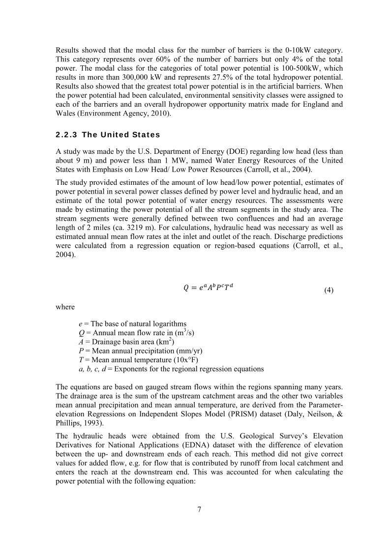
A study was made by the U.S. Department of Energy (DOE) regarding low head (less than about 9 m) and power less than 1 MW, named Water Energy Resources of the United States with Emphasis on Low Head/ Low Power Resources (Carroll, et al., 2004).
The study provided estimates of the amount of low head/low power potential, estimates of power potential in several power classes defined by power level and hydraulic head, and an estimate of the total power potential of water energy resources. The assessments were made by estimating the power potential of all the stream segments in the study area. The stream segments were generally defined between two confluences and had an average length of 2 miles (ca. 3219 m). For calculations, hydraulic head was necessary as well as estimated annual mean flow rates at the inlet and outlet of the reach. Discharge predictions were calculated from a regression equation or region-based equations (Carroll, et al., 2004).
𝑄 = 𝑒𝑎𝐴𝑏𝑃𝑐𝑇𝑑
(4)
where
e = The base of natural logarithms Q = Annual mean flow rate in (m3/s) A = Drainage basin area (km2) P = Mean annual precipitation (mm/yr) T = Mean annual temperature (10x°F) a, b, c, d = Exponents for the regional regression equations
The equations are based on gauged stream flows within the regions spanning many years. The drainage area is the sum of the upstream catchment areas and the other two variables mean annual precipitation and mean annual temperature, are derived from the Parameter-elevation Regressions on Independent Slopes Model (PRISM) dataset (Daly, Neilson, & Phillips, 1993).
The hydraulic heads were obtained from the U.S. Geological Survey’s Elevation Derivatives for National Applications (EDNA) dataset with the difference of elevation between the up- and downstream ends of each reach. This method did not give correct values for added flow, e.g. for flow that is contributed by runoff from local catchment and enters the reach at the downstream end. This was accounted for when calculating the power potential with the following equation:

8
𝑃 = 𝜅 �𝑄𝑖𝐻 + (𝑄𝑜 − 𝑄𝑖)
𝐻2� ; 𝐻 = 𝑧𝑖 − 𝑧𝑜
(5)
where
P = Power (kW) κ = Pressure coefficient value, equals 1/11.8 s/ft4kW Qi = Flow rate at the upstream end of the stream reach (ft3/s) Qo = Flow rate at the downstream end of the stream reach (ft3/s) H = Hydraulic head (ft) zi = Elevation at the upstream end of the stream reach (ft) zo = Elevation at the downstream end of the stream reach (ft)
The (QiH) quantity gives the power potential of the flow that enters at the upstream end of the reach and experiences full hydraulic head. The (Qo-Qi) quantity is the part of flow added by runoff from the particular catchment with different hydraulic head, varying from full head to zero. An average value of H/2 is therefore used for the flow from the local catchment (Carroll, et al., 2004). The pressure coefficient value (κ = gρ) is different for each measurement unit type. This coefficient is defined with the inverse of the 4′th power of the length for a given unit, hence 1/11.82 for US-kW.
Total hydropower potential was calculated by summing the reach power potentials. The study showed that it is possible to estimate the power potential of the United States water energy resources based on the potentials of mathematical analogs of every stream segment in the country (Carroll, et al., 2004).
2.2.4 Norway
Within the Nordic countries Norway has a special interest in evaluating the potential hydropower since 98.5 percent of the electric energy production comes from hydropower (NVE, 2009). Norwegian Water Resources and Energy Directorate (NVE) has for the past years participated in supporting research and development studies with the aim to increase knowledge of possible small hydropower plants and development of technique and knowledge of more efficient and environmentally friendly use of resources. One of these studies is the calculation of the potential for small power plants in Norway (Voksø, Stensby, Mølmann, Tovås, Skau, & Kavli, 2004). The potential for power plants under 1 MW had been estimated to be 3 TWh and the assessment for plants between 1 and 10 MW was 7 TWh with estimations done in the 1980’s and 1990’s. Since there was no project evaluation behind these estimations, a new method was developed through a joint cooperation between NVE and GIS consultants.
All rivers with a slope down to 1/25 were included in the estimation and the head was limited to range from 10 m to 600 m and mean flow in the range from 0.05 to 25 m3/s. For better understanding of these numbers, Table 1 shows the calculated power for minimum, mean and maximum values of both discharge and head according to the Norwegian thresholds, using eq. (1). For minimum discharge (0.05 m3/s), necessary head to produce 50 kW power is 102 m and for minimum head (10 m), necessary discharge is 0.51 m3/s.

9
Table 1: Power calculated using eq. (1), for minimum, mean and maximum values of discharge and head according to the Norwegian thresholds.
Q [m³/s] H [m] P [kW] 0.05 min 10 min 5 0.05 min 600 max 294 0.05 min 300 mean 147 25 max 10 min 2,453 25 max 600 max 147,150 25 max 300 mean 73,575
12.5 mean 10 min 1,226 12.5 mean 600 max 73,575 12.5 mean 300 mean 36,788
Turbine intake capacity was chosen 1.5 times the mean flow and the hydraulic efficiency was set to 0.815. Additionally it was assumed that 70% of the annual discharge could be utilized for power generation. The power potential was then calculated with the equation of theoretical expression for hydropower with added factor of hydraulic efficiency (eq. (2)) with η equal to 0.815. Automatic calculations of head were made every 50 m tracing the river network from outlet to source by using the river network and the terrain model. All cases were identified with slopes over the defined value. The discharge at the top of each case was obtained from a runoff map. All cases, providing sufficient discharge and head to a power plant between 50 kW and 10,000 kW and a specific construction cost of less than 5 kr/kWh (NOK) were included in the potential (Voksø, et al., 2004).
The runoff map was obtained with a distributed version of the HBV-model using 1 km2 square grid cells and monthly runoff data to estimate average annual runoff. The model uses measurements of precipitation and air temperatures as input and has components for accumulation, sub-grid scale distribution and ablation of snow, interception storage, evapotranspiration, groundwater storage and runoff response, lake evaporation and glacier mass balance (Beldring, Engeland, Roald, Sælthun, & Voksø, 2003)
At the end of the project, the total dataset included a terrain model, a river network, a runoff map, a register of catchments (REGINE), register of developed hydropower, a master plan for water resources as well as new hydroelectric projects, a cost basis and maps of power lines and roads.
Results showed the number of identified cases in the analysis to be 45.529, where 20% were identified as acceptable in terms of all requirements. The results were presented via internet on an interactive map, where every identified potential power plant with its theoretical calculated capacity is located. This has been widely used by both the power industry sector and municipalities (Voksø, et al., 2004). Since the Norwegian conditions have some similarities to Icelandic conditions in terms of climate, geographical position and the extensive hydropower proportion of the energy sector, the Norwegian project will be used for comparison with the results of this study in Section 5.2.

10
2.2.5 Status in Iceland
The hydropower potential in Iceland has been evaluated several times since 1920. Jón Þorláksson estimated available hydropower from precipitation and guessed that 26 TWh/yr could be exploited (Tómasson, 1981). Later, Sigurður Thoroddsen estimated the hydropower potential by assuming a number of hydropower plants, evaluating their capacity of power generation and cumulating the power values for total hydropower potential. The results showed 35 TWh/yr and were presented at a conference about energy and industry in 1962 (Tómasson, 1981). These estimations were used for barely twenty years, or until a new method for estimating hydropower was applied and results presented by Haukur Tómasson at an industry conference in 1981. These results are still used as an estimation of hydropower potential in Iceland, and are based on dividing the country into 916 squared cells with average size 130 km2 (Tómasson, 1981). The hydropower was estimated in two different ways, first by calculating potential hydropower of a particular cell where precipitation falls and then by calculating the potential hydropower from the particular cell where the water appears as surface water. The runoff map from Sigurjón Rist (1956) was used to acquire the runoff factor where average runoff for Iceland was estimated 5,500 m3/s. The runoff used was though equal to 5,150 m3/sec as the former estimations were thought to be a bit high.
Calculations were performed with this new method and results presented at an industry conference in 1981 (Tómasson, 1981). The calculations showed that total hydropower potential from precipitation was 252 TWh/yr, where the greatest potential was in the south-east part of Iceland which has extensive glacial coverage and the least potential in the northern- and western part with less precipitation and lower elevation. The calculations for potential hydropower using the second method showed 187 TWh/yr, where the greatest potential was at glacier-margins and springfed areas in the highland. The different results of these two methods (65 TWh/yr) was thought to be due to glaciofluvial and groundwater flow.
In order to estimate the exploitable part of the hydropower potential, special hydropower calculations were made for the bulkier part of the river network, assuming a hydropower plant every 5 km. The calculations assumed 2,200 hydropower plants located in 192 rivers that account for 20% of the total length of the river network. The head for each hydropower plant was limited to 5 meters minimum and the power to 1 MW (8.76 GWh/yr).
The equation used (eq. (6)) was derived by engineers and the National Energy Agency. Results showed 33 TWh/yr of low-cost hydropower potential (Tómasson, 1981). When comparing these past estimations of hydropower potential, it can be seen that the results do only differ from 26 TWh/yr in the year of 1920 to 35 TWh/yr in the year of 1962 and finally 33 TWh/yr in the year of 1981, assuming that all estimations are for exploitable hydropower potential. This implies that the first estimation was quite good since the data was extremely limited. The similarity between the second and the third estimation could be due to the fact that they are based on the same runoff map.

11
32.17 10P MaQ H −= ⋅ ⋅ ⋅ (6) where
P = Power (GWh/yr) MaQ = Annual mean discharge (m3/sec) H = Head (m) Since the last review, numerous things have changed in Iceland regarding quality and development of cartography and database technology with GIS and regarding hydraulic and hydrological researches. A new national hydrological database has been made at the Icelandic Meteorological Office (IMO) where the base is a digital elevation model (DEM) in resolution of 25 m (Björnsson & Jensen, 2010). Hydraulic models have been made for flood assumptions. The knowledge of relative distribution of flow as well as knowledge of groundwater and the hydrology of glaciers is also much better. Additional weather observations have been made in the highlands and measurements of glaciers and snow-tracking have been improved. There has also been a major increase in number of gauges since 1981 (Einarsson, 1999). Last but not least, a major development has taken place regarding hydrological modeling using the WaSiM model, which replaced the HBV model.
The model came first in use for hydrological simulations in Iceland in the making of a runoff map (Jónsdóttir, 2004) and through the Nordic research project, Climate and Energy (CE) (Beldring, et al., 2006). The model was used to make a runoff map of the country for the period 1961-1990 and to map the future projection of runoff for 2071-2100 (Jónsdóttir, 2008). This study did not apply the groundwater model of WaSiM. The model was then used to make future projection of runoff of two catchments in Iceland (Sandá River in Þistilfjörður and Austari-Jökulsá River) for the period 2021-2050 (Einarsson & Jónsson, 2010a). This was done after implemented improvements regarding activation of the groundwater model, seasonal changes in the Hamon evapotranspiration scheme and glacier melt parameters. These studies have all the same input data of precipitation, temperature, vapor pressure, wind and radiation with 8 km resolution (Rögnvaldsson, Jónsdóttir, & Ólafsson, 2007). Recently, further improvements have been implemented in the use of the model, such as simulating the effect of frozen ground, seasonal changes in snowmelt factors and with the use of Penman-Monteith scheme of evapotranspiration instead of using a temperature index method like Hamon. Analyses of results have been made easier applying a semi-automatic calibration through multi-runs (Atladóttir, Crochet, Jónsson, & Hróðmarsson, 2011). In addition, the input data has been improved for precipitation (Crochet, et al., 2007) and temperature (Crochet & Jóhannesson, 2011) which both produce datasets in 1 km resolution (Atladóttir, et al., 2011). With major opportunities of hydropower in Iceland it is important to utilize these improvements and a vital part of that is to make a new map of potential hydropower.


13
3 Model development for assessing Hydropower Potential
In order to estimate hydropower potential, using the theoretical power equation (eq. (1)), head and discharge must be obtained. The assessment of these two variables is therefore the main task of the methodology and is described in Sections 3.1 and 3.2. The calculations of technical hydropower potential are discussed and described in Section 3.3.
3.1 Head
3.1.1 Elevation data
The elevation data is provided with different data grids from the ArcGIS database at the IMO. For the past few years a new national hydrological database, with spatial data, has been made at the IMO in order to fulfill requirements of the EU Water Framework Directive. The database was mainly created from existing hydrological cartographic data as well as with a digital elevation model (DEM). The Hydrological Service (now a part of IMO) obtained a DEM from the Iceland GeoSurvey (ÍSOR) for the new database. The DEM is made from cells, each of size 25x25 m2 and has 10-50 m vertical accuracy. The quality and accuracy of the data varies by region and depends on the origin of the data. The hydrology data was obtained from Loftmyndir ehf, including surface water features such as lakes, streams and river centerlines. (Björnsson, Jensen, Karlsdóttir & Harðardóttir, 2008).
The Icelandic hydrological database is built on the ArcHydro data model which was developed in collaboration with the Environmental Systems Research Institute (ESRI). The model is a geo-database that links hydrologic information to water resources modeling (Maidment, 2002) and is based on simple phenomena, polygons, lines and dots saved in an ESRI geo-database. The model assumes stream lines and catchments which information can be attached to with a unique identification number called HydroID. The DEM is used to determine flow direction and flow accumulation for every cell and these two datasets are used to produce drainage lines, based on a flow accumulation threshold. For every segment of a stream, ArcHydro calculates a catchment based on the flow direction of the cells (Björnsson & Jensen, 2010). This will be further discussed in Section 3.1.2. The result is a national direction-based hydrological network database (Björnsson, et al., 2008) describing runoff attached to the catchment areas through a unique code (HydroID). The runoff is therefore not described in terms of quantity of water but in terms of the flow direction and accumulation. By coupling information from discharge simulations with the hydrological network the quantity of water is displayed (Björnsson & Jensen, 2010).
Different data grids are obtained from the hydrological database for this study; a DEM, a stream grid, a flow accumulation grid, a catchment grid and a stream segmentation grid identifying each segment of the river network. All grids are obtained in an ascii format with cell size 25x25 m2. The DEM shows the elevation of every cell as integers, which means that minimum difference in elevation between cells is limited to 1 m.
14
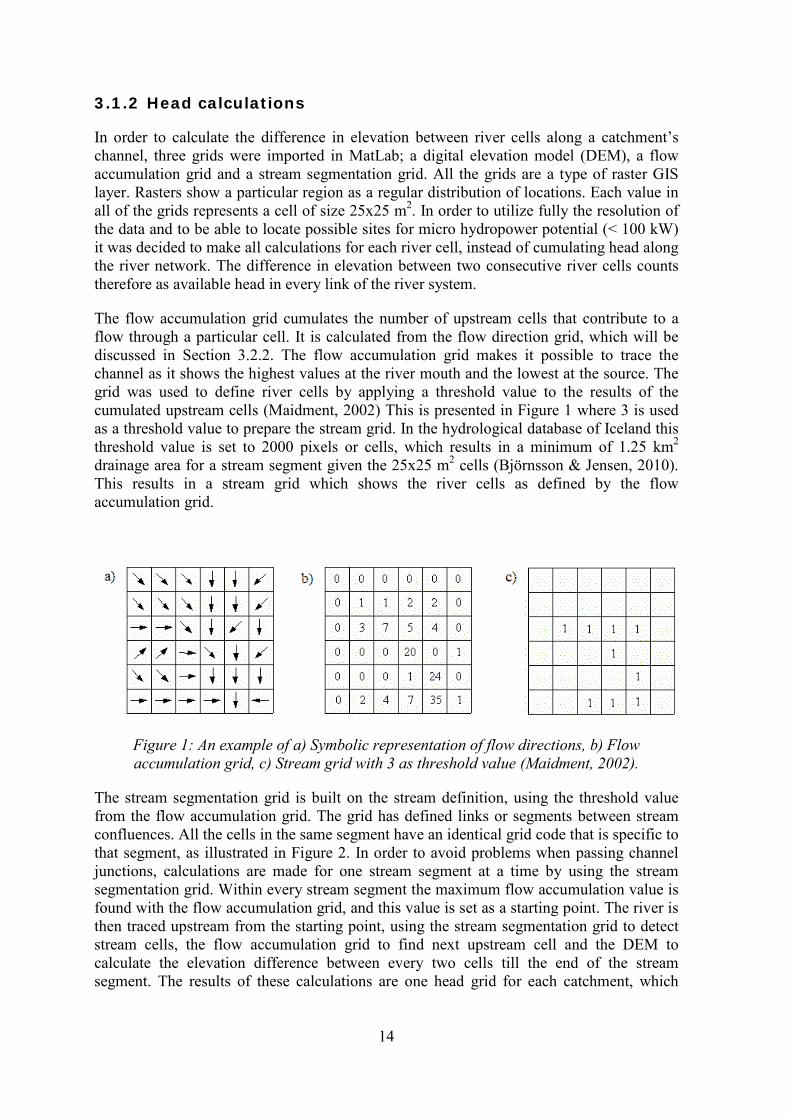
3.1.2 Head calculations
In order to calculate the difference in elevation between river cells along a catchment’s channel, three grids were imported in MatLab; a digital elevation model (DEM), a flow accumulation grid and a stream segmentation grid. All the grids are a type of raster GIS layer. Rasters show a particular region as a regular distribution of locations. Each value in all of the grids represents a cell of size 25x25 m2. In order to utilize fully the resolution of the data and to be able to locate possible sites for micro hydropower potential (< 100 kW) it was decided to make all calculations for each river cell, instead of cumulating head along the river network. The difference in elevation between two consecutive river cells counts therefore as available head in every link of the river system.
The flow accumulation grid cumulates the number of upstream cells that contribute to a flow through a particular cell. It is calculated from the flow direction grid, which will be discussed in Section 3.2.2. The flow accumulation grid makes it possible to trace the channel as it shows the highest values at the river mouth and the lowest at the source. The grid was used to define river cells by applying a threshold value to the results of the cumulated upstream cells (Maidment, 2002) This is presented in Figure 1 where 3 is used as a threshold value to prepare the stream grid. In the hydrological database of Iceland this threshold value is set to 2000 pixels or cells, which results in a minimum of 1.25 km2 drainage area for a stream segment given the 25x25 m2 cells (Björnsson & Jensen, 2010). This results in a stream grid which shows the river cells as defined by the flow accumulation grid.
Figure 1: An example of a) Symbolic representation of flow directions, b) Flow accumulation grid, c) Stream grid with 3 as threshold value (Maidment, 2002).
The stream segmentation grid is built on the stream definition, using the threshold value from the flow accumulation grid. The grid has defined links or segments between stream confluences. All the cells in the same segment have an identical grid code that is specific to that segment, as illustrated in Figure 2. In order to avoid problems when passing channel junctions, calculations are made for one stream segment at a time by using the stream segmentation grid. Within every stream segment the maximum flow accumulation value is found with the flow accumulation grid, and this value is set as a starting point. The river is then traced upstream from the starting point, using the stream segmentation grid to detect stream cells, the flow accumulation grid to find next upstream cell and the DEM to calculate the elevation difference between every two cells till the end of the stream segment. The results of these calculations are one head grid for each catchment, which
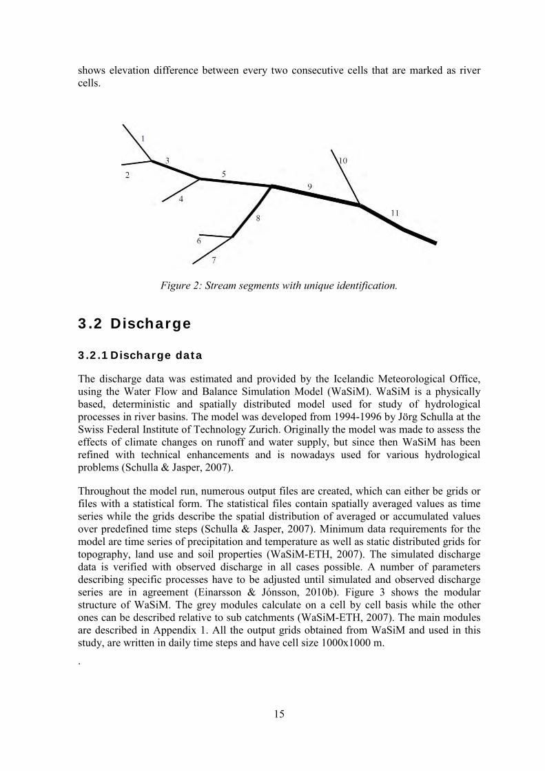
15
shows elevation difference between every two consecutive cells that are marked as river cells.
Figure 2: Stream segments with unique identification.
3.2 Discharge
3.2.1 Discharge data
The discharge data was estimated and provided by the Icelandic Meteorological Office, using the Water Flow and Balance Simulation Model (WaSiM). WaSiM is a physically based, deterministic and spatially distributed model used for study of hydrological processes in river basins. The model was developed from 1994-1996 by Jörg Schulla at the Swiss Federal Institute of Technology Zurich. Originally the model was made to assess the effects of climate changes on runoff and water supply, but since then WaSiM has been refined with technical enhancements and is nowadays used for various hydrological problems (Schulla & Jasper, 2007).
Throughout the model run, numerous output files are created, which can either be grids or files with a statistical form. The statistical files contain spatially averaged values as time series while the grids describe the spatial distribution of averaged or accumulated values over predefined time steps (Schulla & Jasper, 2007). Minimum data requirements for the model are time series of precipitation and temperature as well as static distributed grids for topography, land use and soil properties (WaSiM-ETH, 2007). The simulated discharge data is verified with observed discharge in all cases possible. A number of parameters describing specific processes have to be adjusted until simulated and observed discharge series are in agreement (Einarsson & Jónsson, 2010b). Figure 3 shows the modular structure of WaSiM. The grey modules calculate on a cell by cell basis while the other ones can be described relative to sub catchments (WaSiM-ETH, 2007). The main modules are described in Appendix 1. All the output grids obtained from WaSiM and used in this study, are written in daily time steps and have cell size 1000x1000 m.
.

16
Figure 3: Modular structure of WaSiM (Allgemeine Modellstruktur, 2007).
Input of meteorological data
Interpolation of meteorological data
Shadowing and exposition dependent adjustment for radiation and temperature
Potential and real evapotranspiration
Snow accumulation and snow melt Glacier model
Interception
Infiltration/generation of surface runoff
Soil(root)storage and unsaturated zone
Saturated zone
Discharge routing
Generating surface runoff
Generating interflow
Generating baseflow
Total discharge
Evaporatiom from snow surfaces
Evaporation from the interception storage
Evapotranspiration from the soil and
from the vegetation
Layers

17
3.2.2 Discharge estimations
Daily river discharge was simulated with the hydrological model WaSiM (see Appendix I) as discussed in Section 3.2.1. A 10 year simulation period was chosen from 1992 to 2001, with the aim to use recent data and to keep the period long enough for the results to be reliable without being a setback for the project regarding data amount.
The WaSiM model provides gridded runoff data where each grid cell represents 1000x1000 m. Three different runoff grids were written per day to form total runoff, baseflow, interflow and surface runoff, illustrated in Figure 4. In catchments with glacial coverage, three extra grids were written per day to obtain total runoff; melt from ice, melt from firn and snowcover runoff. All the data were provided in millimeters for each grid cell and for each day
Figure 4: A schematic of the three runoff components forming total runoff.
With the purpose of acquiring runoff data for every grid cell along the river network, it is necessary to route the water. This was done by using the flow accumulation tool from ArcGIS 9.3 to refer the runoff values into right places. The flow accumulation is calculated from the flow direction grid, which is based on a digital elevation model. It is assumed that every cell flows towards one of its neighboring cells depending on the steepness in the digital elevation map. The slope is defined by elevation decrease per unit travel distance and the water will flow to the steepest direction, presented with a flow direction code (Figure 5-b) (Maidment, 2002). Figure 5 illustrates the process from a DEM to a symbolic representation of flow directions for the DEM. The necessary datasets were obtained from the Icelandic hydrological database, as discussed in Section 3.1.1.
In order to use the flow direction grid and to be able to couple the elevation data with the discharge data later on, the 1000x1000 m2 runoff data had to be redistributed on the 25x25 m2 cells. Every 1000x1000 m2 cell was divided into 1600 cells of size 25x25 m2 and the runoff value of the original cell was assigned to all of them. Instead of using the flow accumulation function to show the number of cells upstream of each cell, the runoff of each cell was defined as weight, in which case the weights were summed for all upstream cells (Maidment, 2002). A script was used to run the flow accumulation function repeatedly for every day through the 10 year period. Using this method, no recession was

18
accounted for. This means that the entire volume of water is routed within 24 hours, no matter the location of the cell on the catchment. The same method may be used in catchments with manmade discharge regulations aboveground but since no underground discharge regulations have been assumed in the Icelandic hydrological database, routing through tunnels has to be done manually.
Figure 5: An example of: a) Digital elevation map, b) Flow direction code , c) Flow direction grid and d) Symbolic representation of flow directions (Maidment, 2002).
When all the runoff data had been routed for each day of the whole period, the mean runoff was calculated for each grid cell marked as river cell, as well as different quantiles of a flow duration curve (FDC). A FDC provides an estimate of the percentage of time a given runoff was equaled or exceeded over defined period, as discussed in Section 2.2, in this case the 10 year simulation period. Figure 6 shows an example of a FDC, made with discharge observations. The lowest quantiles of the FDC represent the flood peaks of the discharge serie and the highest quantiles represent the extreme low flows. This is illustrated with symbols in Figure 6, where the 90% quantile of the FDC corresponds to 1 m3/s and the 20% quantile to 5 m3/s. The mean discharge and as well as FDC quantiles from 10%-95% were calculated and used in this study as discharge estimation to be used in eq. (1). The selection of the quantiles used will be further discussed in Section 3.3.
In order to study the benefit of using an advanced hydrological model such as WaSiM, the discharge estimation was compared with gridded precipitation data which were directly used as a proxy for runoff. The runoff from precipitation was therefore used without performing any hydrological simulations or taking into account any hydrological processes

19
such as snow storage, evaporation and infiltration. The simulated gridded runoff and the runoff from precipitation were routed in the same manner.
Figure 6: An example of a flow duration curve, made from discharge observations.
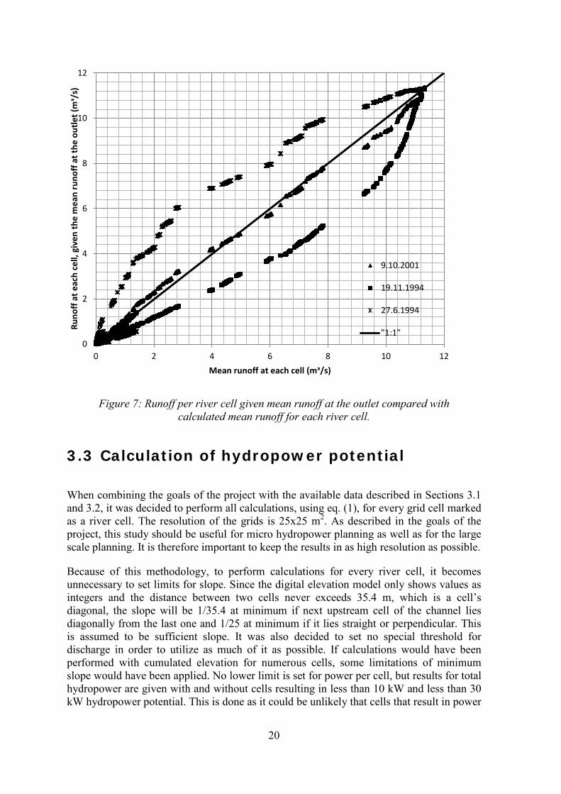
When the FDCs were calculated for this study, two methodologies were considered. In the first one, a specific FDC was made for every single river cell in the catchment. In the second one, the FDC was calculated at the outlet only, and then the day, for which the observed discharge corresponding to each quantile, was selected, and the upstream discharge used.
These two different approaches of calculating the FDCs were tested for one particular catchment and the result is illustrated in Figure 7. The figure shows runoff at each river cell in the catchment. The x-axis shows results according the first method and the y-axis shows results according to the second method. Runoff data for three different days, that all result in the same mean runoff at the outlet, is plotted against the mean runoff calculated for each cell. The 1:1 line shows the perfect fit between the different approaches. The results for the different days illustrate that different scenarios within the catchment can cause the same discharge at the outlet. This shows that the second method, where the FDC is only calculated at the river outlet, can give inaccurate discharge information along the river network. The method used is therefore the first method as it has the advantage of providing precise information for every tributary. It is though noted that calculating only a FDC at the outlet could in some cases be sufficient and would reduce the processing time.
0
5
10
15
20
25
30
0 10 20 30 40 50 60 70 80 90 100
m3
/s
Percent of time
20
Figure 7: Runoff per river cell given mean runoff at the outlet compared with calculated mean runoff for each river cell.
3.3 Calculation of hydropower potential When combining the goals of the project with the available data described in Sections 3.1 and 3.2, it was decided to perform all calculations, using eq. (1), for every grid cell marked as a river cell. The resolution of the grids is 25x25 m2. As described in the goals of the project, this study should be useful for micro hydropower planning as well as for the large scale planning. It is therefore important to keep the results in as high resolution as possible.
Because of this methodology, to perform calculations for every river cell, it becomes unnecessary to set limits for slope. Since the digital elevation model only shows values as integers and the distance between two cells never exceeds 35.4 m, which is a cell’s diagonal, the slope will be 1/35.4 at minimum if next upstream cell of the channel lies diagonally from the last one and 1/25 at minimum if it lies straight or perpendicular. This is assumed to be sufficient slope. It was also decided to set no special threshold for discharge in order to utilize as much of it as possible. If calculations would have been performed with cumulated elevation for numerous cells, some limitations of minimum slope would have been applied. No lower limit is set for power per cell, but results for total hydropower are given with and without cells resulting in less than 10 kW and less than 30 kW hydropower potential. This is done as it could be unlikely that cells that result in power
0
2
4
6
8
10
12
0 2 4 6 8 10 12
Runo
ff at
eac
h ce
ll, g
iven
the
mea
n ru
noff
at th
e ou
tlet (
mᶟ/
s)
Mean runoff at each cell (mᶟ/s)
9.10.2001
19.11.1994
27.6.1994
"1:1"

21
of this degree, especially under 10 kW, will be utilized, and also to see the proportion of these low power cells compared to the total hydropower potential of the catchment.
The methodology used, represents the technical hydropower potential, which means all potential hydropower without any abstractions, for example due to losses in pipes or environmental conservation, etc. The efficiency factor is not estimated in this study for the same reason and is therefore kept as 100%. Calculated head and routed runoff were used to calculate the hydropower potential for each river cell by applying eq. (1), considering mean discharge and several runoff quantiles from the FDCs. The same calculations were also performed using routed precipitation as discharge estimation for comparison, as discussed in Section 3.2.2. The different discharge inputs can be seen in Table 2. The higher quantiles (65% and above) are calculated in order to estimate the potential for run-of-river projects where low flow is normally used, and the mean is used in order to estimate the hydropower potential assuming a storage project using reservoir to regulate the water. The 50% quantile could be interesting for both storage- and run-of-river projects. The lowest quantile (10%) is calculated to see what to expect for the highest components of the discharge, although the flood peaks are seldom utilized, especially in run-of-river projects. Good quality turbines can though in some cases operate over a range of flow rates, from high flow down to one-sixth of the high flow (Renewables First Ltd., 2011). It is therefore necessary to analyze the contribution of different flow rates to potential hydropower. For further processing, it would be necessary to account for retaining minimum discharge in the channel for ecological reasons.
Table 2: Different use of discharge inputs for calculating the technical hydropower potential.
Discharge input Usage Mean runoff Storage projects 95% FDC Run-of-river projects 85% FDC Run-of-river projects 75% FDC Run-of-river projects 65% FDC Run-of-river projects 50% FDC Run-of-river and storage projects 10% FDC Analyze the flood peaks
A storage hydropower project impounds and stores water in a reservoir during high-flow periods to increase the water available during low-flow periods, allowing the flow releases and power production to be more constant. This would be more convenient where low-flow based capacity is not sufficient. It is though vital to keep in mind that the structure of a dam and reservoir can be expensive and will have environmental impacts.
The part of the FDC that covers 50-100% duration may be considered as the low flow section where the range of 70-99% duration are most widely used as design low flows (Smakhtin, 2001). As mentioned above, this low flow part can be of special interest regarding further processing of potential hydropower production, since it can be used to represent the proportion of stream flow originating from groundwater stores, separating the base flow component. The base flow often represents the minimal volume of water required for the river to maintain ecological health and stability, e.g. in terms of habitats

22
(Department of the Environment, Climate change, Energy and Water, 2009), and is therefore not optimal for use in hydropower planning.
Total hydropower potential can be calculated for different quantiles of the FDC for each catchment by cumulating the power values along the river network. As it may be unrealistic to keep no lower limit on hydropower per cell in the total sum up, results for total hydropower are also given when all cells resulting in hydropower potential less than 10 kW and less than 30 kW have been excluded. All river cells that carry 10-30 kW, 31-50 kW, 51-100 kW, 101-1000 kW and 1001-5000 kW are registered and mapped for visualization. For the larger catchments, river cells that carry more than 5000 kW are also registered and mapped. The larger power categories (101 – 1000 kW and 1001 – 5000 kW) have quite extensive range, this was done as the mapping was more intended to identify potential sites for small scale hydropower rather than the large scale that has in most cases already been investigated up to some extent. This is only for the visual presentations but all calculations hold the exact kW per river cell. Further analyses of possible locations of hydropower plants are not investigated in this study.
These calculations will result in a database that carries an estimation of the hydropower potential for each river cell in the whole catchment, calculated for run-of-river and storage projects, by assuming mean discharge and different quantiles of a FDC. It is noted that no hydropower potential will be calculated directly on glaciers, since the stream grid does not show any river cells on glaciers. Discharge from the glaciers is though accounted for since the flow accumulation grid accumulates discharge from the glacier. All the results of this study will be stored at the IMO.
23
4 Model adaptation on three different catchments in Iceland When choosing the catchments to use in this study for testing of the methodology, availability of data was limited. Recent improvements in the hydrological model WaSiM have only been applied to catchments in the western part of Iceland (Vestfirðir), but a part of the project’s aims was to test the methodology for different parts of the country. Taking that into consideration, the catchment of Dynjandisá River was chosen from Vestfirðir and also the two catchments that have been simulated using the groundwater model but without recent improvements in WaSiM, Sandá River in Þistilfjörður and Austari-Jökulsá River. The runoff data used in calculations for the Dynjandisá River is simulated using all the recent improvements described in Section 2.2.5. It may therefore be assumed that the discharge estimation should be more accurate for the catchment of Dynjandisá River than for the other two catchments. These three catchments are used for testing of the methodology presented in Chapter 3 and results are presented in the following sections. The 10 year simulation period is chosen the same for all three catchments as discussed in Section 3.2.2.
The hydropower potential calculations for the catchment of Dynjandisá River are performed assuming mean discharge and repeated for each chosen quantile of the FDC as discussed in Section 3.3. All the results are presented on maps in order to identify if all of the different quantiles of the FDC are necessary for analyzing hydropower potential. The calculations for Sandá River and Austari-Jökulsá River are also performed assuming mean discharge and for each chosen quantile of the FDC, but the results are only mapped assuming mean discharge and the 75% quantile. The mean discharge is used for estimating the hydropower potential assuming storage projects and the 75% quantile is used for estimating the potential assuming run-of-river projects. For each catchment, the calculations of hydropower potential are summarized and the discharge estimations are compared with gridded precipitation data which are directly routed and used as a proxy for runoff without using WaSiM, as discussed in Section 3.2.2.

24
4.1 Dynjandisá River The catchment of Dynjandisá River is located in the northwest of Iceland and has an area of 43 km2 (Icelandic Meteorological Office, 2011a). The location of the catchment can be seen in Figure 8. The source of Dynjandisá River is at the lakes of Dynjandisheiði Highlands where it runs from a mountain ridge in series of waterfalls before it reaches sea. Dynjandisá River is a direct runoff river with a small spring-fed part and is regulated by small lakes (Icelandic Meteorological Office, 2011a). Discharge rating curves, corresponding to the water-level gauge in Dynjandisá River are available from the beginning of continuous measurements in 1956 (Icelandic Meteorological Office, 2011a).
Figure 8: Location of the catchment of Dynjandisá River.
Table 3 shows a comparison of observed and simulated discharge at the water level gauge for the simulation period 1992-2001. The table also shows observed discharge for a longer discharge serie from 1961 to 2002. It can be seen that the observed discharge serie for the simulation period should give a sufficient estimation of the long-run mean discharge for Dynjandisá River, although the minimum and maximum daily discharge differs between the simulation period and the longer discharge serie. For the simulated discharge, the table shows that the mean discharge is in line with the mean observed one and the maximum simulated discharge is consistent with the observed maximum. The minimum simulated discharge is too high compared to the minimum observed discharge due to difficulties of simulating discharge in extreme low flows. This could cause an overestimated hydropower potential for the higher quantiles (low flow).
Figure 9 shows the FDC for Dynjandisá River, according to simulated discharge at the outlet of the catchment. The mean simulated discharge corresponds to the 35% quantile of the FDC for the same period, which means that for 35% of the simulation period, 3.13 m3/s are equaled or exceeded.

25
Table 3: Comparison of observed and simulated discharge at the water level gauge in Dynjandisá River.
Mean daily discharge (mᶟ/s)
Observations Simulations
1961-2002 1992-2001 1992-2001 mean 3.02 3.17 3.13 min 0.1 0.14 0.8 max 35.4 25.4 24.4
Figure 9: A FDC for Dynjandisá River (vhm 19), the discharge is simulated at the catchment’s outlet over the simulation period.
4.1.1 Head
The head grid shows elevation difference between river cells along the channel. For Dynjandisá River, the maximum elevation difference between two consecutive river cells is 26 m and the cumulated head along the river network is 1050 m. Difference between the lowest and the highest point is 861 m according to the digital elevation model. The cumulated head gives not the same result as the difference between the lowest and the highest point, since the cumulated head is calculated along the whole river network, including all tributaries. Figure 10 shows cumulated elevation difference between river cells from source to river outlet where the cumulated head equals 1050 m. It can be seen that the main tributaries have cumulated head up to about 200 m each, marked in blue. The river channel downstream of the tributaries has around 400 m of cumulated head before it reaches sea, illustrated in yellow, orange and red. The figure presents the x- and y-axis in number of grid cells where one grid cell is of size 25x25 m2.
0
5
10
15
20
25
30
0% 20% 40% 60% 80% 100%
Disc
harg
e (m
ᶟ/s)
Percentage of time
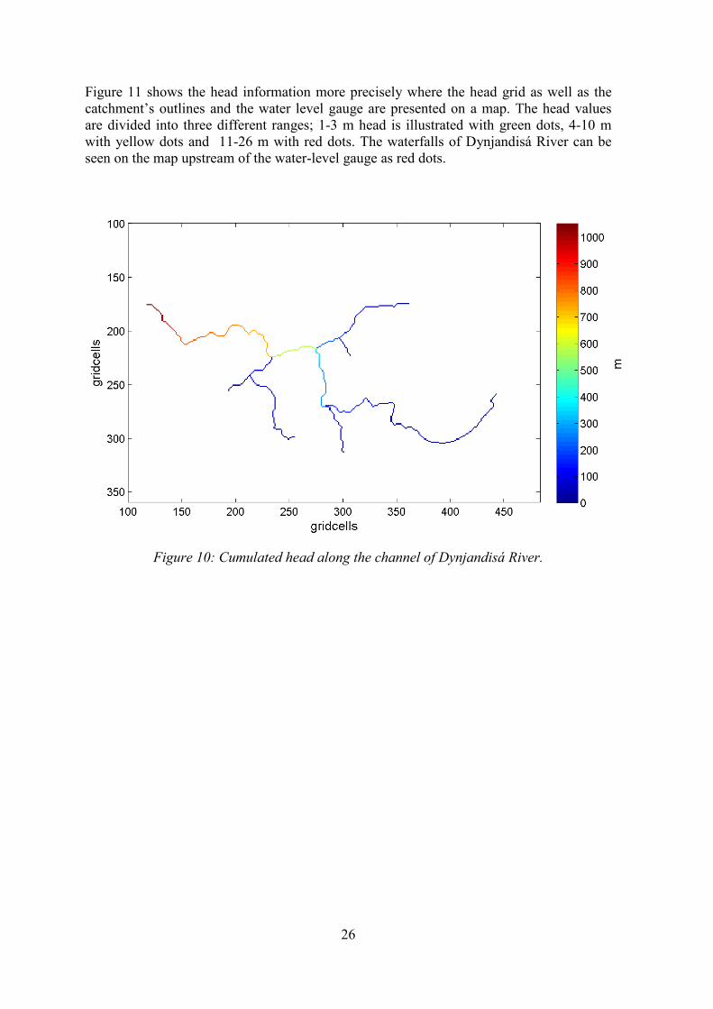
26
Figure 11 shows the head information more precisely where the head grid as well as the catchment’s outlines and the water level gauge are presented on a map. The head values are divided into three different ranges; 1-3 m head is illustrated with green dots, 4-10 m with yellow dots and 11-26 m with red dots. The waterfalls of Dynjandisá River can be seen on the map upstream of the water-level gauge as red dots.
Figure 10: Cumulated head along the channel of Dynjandisá River.

27
Figure 11: The head grid for Dynjandisá River presented on a map.
4.1.2 Hydropower potential
The results of the estimation of technical hydropower potential for Dynjandisá River are presented assuming first mean discharge and then six different quantiles of the FDC, as discussed in Section 3.3. Since the calculations are repeated for each quantile, the results assuming mean runoff and the first quantile are explained in details, but the results of the other 5 runoff scenarios are presented with less detailed explanations. This is done in order to prevent repeating the same explanations in each section. The discharge estimations span extreme low flows, represented with the 95% quantile of the FDC, to extreme high flows, represented with the 10% quantile of the FDC. The runoff data used in calculations for the catchment are provided using recent improvements in WaSiM, as discussed in the beginning of Chapter 4.
Hydropower potential given mean runoff The mean runoff for the 10 year simulation period is 3.13 m3/s, according to simulated discharge at the outlet. Figure 12 shows progression of the mean simulated runoff along the Dynjandisá River network. The tributaries are illustrated in blue as they only have mean runoff from 0 to 1 m3/s. The outlet of the main channel is illustrated in red as it has more than 3 m3/s as mean runoff.
The hydropower calculations assuming mean runoff result in a total power of 13,575 kW where the maximum power value is calculated 785 kW per single cell. Figure 13 illustrates the hydropower accumulation along the river network with the same color bar as for Figure

28
12, from blue for low values to red for high values. The tributaries are illustrated in blue but the main channel downstream of the tributaries goes from light blue to red color at the outlet where it reaches 13,575 kW. Table 4 shows the total resulting power, cumulated along the river network. The last two columns give the results of total cumulated power where river cells resulting in less than 10 kW and 30 kW are excluded. If all river cells resulting in hydropower potential less than 10 kW are excluded, the result will show total power of 12,958 kW, or about 5% less than the total cumulated power for all the river cells. When river cells resulting in less than 30 kW are excluded, the result of total power will show 11,094 kW, or about 18% less than the original value of cumulated power. This illustrates that up to 18% of the total cumulated power, estimated assuming mean runoff, originates from river cells with such low power that it may in some cases be difficult to utilize.
Table 4: The total resulting hydropower potential in Dynjandisá River, assuming mean runoff.
All cells < 10 kW excluded < 30 kW excluded
Total power [kW] 13,575 12,958 11,094
Table 5 presents the number of river cells resulting in specific range of power as discussed in Section 3.3, assuming mean runoff. Most of the river cells have potential hydropower in the range of 1-10 kW and no cell has more than 785 kW as hydropower potential. This is also presented in Figure 14, where the results of the hydropower potential calculations as well as the catchment’s outlines and the water level gauge are presented on a map. A more detailed analysis of the results is presented in Appendix II (Figure 50 and Figure 51). The power values are divided into five different ranges; 10-30 kW are illustrated with green dots, 31-50 kW with light green dots, 51-100 kW with yellow dots, 101-1000 kW with orange dots and 1001-5000 kW with red dots. The waterfalls of Dynjandisá River can be seen on the map upstream of the water-level gauge as orange dots.
Table 5: The number of cells within the range of defined values of hydropower potential calculated with mean discharge.
Power (kW) 0-10 10-30 30-50 50-100 100-1000 1000-5000
Cell (number) 146 95 26 26 33 0
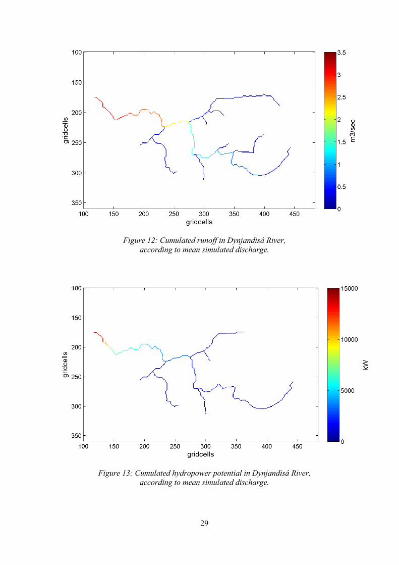
29
Figure 12: Cumulated runoff in Dynjandisá River, according to mean simulated discharge.
Figure 13: Cumulated hydropower potential in Dynjandisá River, according to mean simulated discharge.

Figure 14: Results of the estimated technical hydropower potential for the catchment of Dynjandisá River, according to mean discharge. The two domains marked with number 1 and 2 represent the outlines of two other maps, presented in Appendix II.
30

31
Hydropower potential given 95% FDC The 95% quantile of the FDC is chosen to represent the extreme low flow and equals 0.9 m3/s, simulated at the outlet of the catchment. Figure 15 shows progression of the 95% quantile along the Dynjandisá River network. The total river network is illustrated in blue as no river cell exceeds 1 m3/s. The hydropower calculations assuming 95% quantile of the FDC result in a total power of 3,535 kW where the maximum power value is calculated 222 kW per single cell. Figure 16 illustrates the hydropower accumulation along the river network with the same colorbar as for Figure 15, from blue for low values to red for high values. Most of the river network is illustrated in blue since the discharge is estimated extremely low. Table 6 shows the total resulting power, cumulated along the river network. The last two columns give the results of total cumulated power where river cells resulting in less than 10 kW and 30 kW are excluded. If all river cells resulting in hydropower potential less than 10 kW are excluded, the result will show about 20% less than the total cumulated power for all the river cells. When river cells resulting in less than 30 kW are excluded, the result of total power will show about 37% less than the original value of cumulated power. This illustrates that up to 37% of the total cumulated power, estimated assuming 95% quantile of the FDC, originates from river cells with such low power that it may in some cases be difficult to utilize.
Table 6: The total resulting hydropower potential in Dynjandisá River, assuming the 95% quantile of the FDC.
All cells < 10 kW excluded < 30 kW excluded
Total power [kW] 3,535 2,842 2,243
Table 7 presents the number of river cells resulting in specific range of power as discussed in Section 3.3, assuming the 95% quantile of the FDC. Most of the river cells have potential hydropower in the range of 1-10 kW and no cell has more than 222 kW as hydropower potential. This is also presented in Figure 17, where the results of the hydropower potential calculations as well as the catchment’s outlines and the water level gauge are presented on a map. A more detailed analysis of the results is presented in Appendix II (Figure 52 and Figure 53). The power values are divided into five different ranges; 10 – 30 kW are illustrated with green dots, 31 – 50 kW with light green dots, 51 – 100 kW with yellow dots, 101 – 1000 kW with orange dots and 1001 – 5000 kW with red dots. It can be seen that the hydropower potential is quite low according to these estimations. Only few river cells result in any hydropower potential and most of them are located near the waterfalls upstream of the water level gauge.
Table 7: The number of cells within the range of defined values of hydropower potential calculated with 95% FDC.
Power (kW) 0-10 10-30 30-50 50-100 100-1000 1000-5000
Cell (number) 260 35 12 13 6 0

32
Figure 15: Cumulated runoff in Dynjandisá River, according to the 95% quantile of the FDC.
Figure 16: Cumulated hydropower potential in Dynjandisá River, according to the 95% quantile of the FDC.

Figure 17: Results of the estimated technical hydropower potential for the Dynjandisá River, according to the 95% quantile of the FDC. The two domains marked with number 1 and 2 represent the outlines of two other maps, presented in Appendix II.
33

34
Hydropower potential given 85% FDC The 85% quantile of the FDC is one of the quantiles chosen to represent the low flow and equals 1.01 m3/s, simulated at the outlet of the catchment. Figure 18 shows the 85% quantile of the FDC for each river cell in the Dynjandisá River network. The total river network is illustrated in blue to light blue and green where the color green represents 1 m3/s. The 85% quantile results in total power of 3,991 kW where the maximum power value is calculated 250 kW per single cell. Figure 19 illustrates the hydropower accumulation along the river network. Most of the river network is illustrated in blue as in Figure 16 for the 95% quantile of the FDC. Table 8 shows the total resulting power, cumulated along the river network. The table also illustrates that up to 37% of the total cumulated power, originates from river cells with power lower than 30 kW, which may in some cases be difficult to utilize. This is the same result as for the 95% FDC.
Table 8: The total resulting hydropower potential in Dynjandisá River, assuming the 85% quantile of the FDC.
All cells < 10 kW excluded < 30 kW excluded
Total power [kW] 3,991 3,234 2,526
Table 9 presents the number of river cells resulting in specific range of power as discussed in Section 3.3, assuming the 85% quantile of the FDC. Most of the river cells have potential hydropower in the range of 1-10 kW and no cell has more than 250 kW as hydropower potential. This is also presented in Figure 20, in form of a map, and in more details in Appendix II (Figure 54 and Figure 55). It can be seen that the location of river cells with hydropower potential is still mainly around the waterfalls upstream of the water level gauge.
Table 9: The number of cells within the range of defined values of hydropower potential calculated with 85% FDC.
Power (kW) 0-10 10-30 30-50 50-100 100-1000 1000-5000
Cell (number) 256 39 11 13 7 0

35
Figure 18: Cumulated runoff in Dynjandisá River, according to the 85% quantile of the FDC.
Figure 19: Cumulated hydropower potential in Dynjandisá River, according to the 85% quantile of the FDC.

Figure 20: Results of the estimated technical hydropower potential for the Dynjandisá River, according to the 85% quantile of the FDC. The two domains marked with number 1 and 2 represent the outlines of two other maps, presented in Appendix II.
36

37
Hydropower potential given 75% FDC The 75% quantile of the FDC is one of the quantiles chosen to represent the low flow and equals 1.11 m3/s, simulated at the outlet of the catchment. Figure 21 shows the 75% quantile of the FDC for each river cell in the Dynjandisá River network. The 75% quantile results in total power of 4,372 kW where the maximum power value is calculated 273 kW per single cell. Figure 22 illustrates the hydropower accumulation along the river network. The main channel downstream of the tributaries is illustrated in light blue to red at the outlet where the accumulated hydropower reaches 4,372 kW. Table 10 shows the total resulting power, cumulated along the river network. The table also shows that up to 28% of the total cumulated power, estimated assuming 75% quantile of the FDC, originates from river cells with power lower than 30 kW, which may in some cases be difficult to utilize.
Table 10: The total resulting hydropower potential in Dynjandisá River, assuming the 75% quantile of the FDC.
All cells < 10 kW excluded < 30 kW excluded
Total power [kW] 3,991 3,614 2,885
Table 11 presents the number of river cells resulting in specific range of power as discussed in Section 3.3, assuming the 75% quantile of the FDC. Most of the river cells have potential hydropower in the range of 1-10 kW and no cell has more than 273 kW as hydropower potential. This is also presented in Figure 23, in form of a map, and in more details in Appendix II (Figure 56 and Figure 57). It can be seen that the location of river cells with hydropower potential is similar to the results of hydropower potential estimation assuming 85% and even 95% quantile of the FDC.
Table 11: The number of cells within the range of defined values of hydropower potential calculated with 75% FDC.
Power (kW) 0-10 10-30 30-50 50-100 100-1000 1000-5000
Cell (number) 248 43 13 14 8 0

38
Figure 21: Cumulated runoff in Dynjandisá River, according to the 75% quantile of the FDC.
Figure 22: Cumulated hydropower potential in Dynjandisá River, according to the 75% quantile of the FDC.

Figure 23: Results of the estimated technical hydropower potential for Dynjandisá River, according to the 75% quantile of the FDC. The two domains marked with number 1 and 2 represent the outlines of two other maps, presented in Appendix II.
39

40
Hydropower potential given 65% FDC The 65% quantile of the FDC is chosen to represent upper limit of the low flow and equals 1.26 m3/s, simulated at the outlet of the catchment. Figure 24 shows the 65% quantile of the FDC for each river cell in the Dynjandisá River network. The 65% quantile results in total power of 4,984 kW where the maximum power value is calculated 310 kW per single cell. Figure 25 illustrates the hydropower accumulation along the river network. The main channel downstream of the tributaries is illustrated in light blue to red at the outlet where the accumulated hydropower reaches 4,984 kW. Table 12 shows the total resulting power, cumulated along the river network. The table also shows that up to 32% of the total cumulated power originates from river cells with power lower than 30 kW, which may in some cases be difficult to utilize
Table 12: The total resulting hydropower potential in Dynjandisá River, assuming the 65% quantile of the FDC.
All cells < 10 kW excluded < 30 kW excluded
Total power [kW] 4,984 4,179 3,411
Table 13 presents the number of river cells resulting in specific range of power as discussed in Section 3.3, assuming the 65% quantile of the FDC. Most of the river cells have potential hydropower in the range of 1-10 kW and no cell has more than 310 kW as hydropower potential. This is also presented in Figure 26, in form of a map, and in more details in Appendix II (Figure 58 and Figure 59). It can be seen that the location of river cells with hydropower potential is still similar to the results of hydropower potential estimation assuming the other low flow quantiles; 75%, 85% and 95%.
Table 13: The number of cells within the range of defined values of hydropower potential calculated with 65% FDC.
Power (kW) 0-10 10-30 30-50 50-100 100-1000 1000-5000
Cell (number) 241 46 15 15 9 0

41
Figure 24: Cumulated runoff in Dynjandisá River, according to the 65% quantile of the FDC.
Figure 25: Cumulated hydropower potential in Dynjandisá River, according to the 65% quantile of the FDC.

Figure 26: Results of the estimated technical hydropower potential for Dynjandisá River, according to the 65% quantile of the FDC. The two domains marked with number 1 and 2 represent the outlines of two other maps, presented in Appendix II.
42

43
Hydropower potential given 50% FDC The 50% quantile of the FDC is chosen as it can be useful discharge estimation for both run-of-river and storage projects. The 50% quantile equals 1.8 m3/s, simulated at the outlet of the catchment. Figure 27 shows the 50% quantile of the FDC for each river cell in the Dynjandisá River network. The 50% quantile results in total power of 7,273 kW where the maximum power value is calculated 445 kW per single cell. Figure 28 illustrates the hydropower accumulation along the river network. The maximum value of the color scale is now 7500 kW instead of 5000 kW before. The main channel downstream of the tributaries is illustrated in light blue to red at the outlet where the accumulated hydropower reaches 7,273 kW. Table 14 shows the total resulting power, cumulated along the river network. The table shows that up to 27% of the total cumulated power originates from river cells with power lower than 30 kW, which may in some cases be difficult to utilize
Table 14: The total resulting hydropower potential in Dynjandisá River, assuming the 50% quantile of the FDC.
All cells < 10 kW excluded < 30 kW excluded
Total power [kW] 7,273 6,621 5,288
Table 15 presents the number of river cells resulting in specific range of power as discussed in Section 3.3, assuming the 50% quantile of the FDC. Most of the river cells have potential hydropower in the range of 1-10 kW and no cell has more than 445 kW as hydropower potential. This is also presented in Error! Reference source not found., in form of a map, and in more details in Appendix II (Figure 60 and Figure 61). It can be seen that some hydropower potential is now upstream from Eyjarvatn Lake and the number of orange colored dots has increased in the waterfalls around the water level gauge.
Table 15: The number of cells within the range of defined values of hydropower potential calculated with 50% FDC.
Power (kW) 0-10 10-30 30-50 50-100 100-1000 1000-5000
Cell (number) 196 81 14 15 20 0

44
Figure 27: Cumulated runoff in Dynjandisá River, according to the 50% quantile of the FDC.
Figure 28: Cumulated hydropower potential in Dynjandisá River, according to the 50% quantile of the FDC.

Figure 29: Results of the estimated technical hydropower potential for the Dynjandisá River, according to the 50% quantile of the FDC. The two domains marked with number 1 and 2 represent the outlines of two other maps, presented in Appendix II.
45

46
Hydropower potential using 10% of the flow duration curve The 10% quantile of the FDC is chosen as discharge estimation for flow tops. The 10% quantile equals 6.88 m3/s, simulated at the outlet of the catchment. Figure 30 shows the 10% quantile of the FDC for each river cell in the Dynjandisá River network, with colorbar from blue to red for 0 – 10 m3/s instead of 0 – 2 m3/s. The 10% quantile results in total power of 30,359 kW where the maximum power value is calculated 1,713 kW per single cell. Figure 31 illustrates the hydropower accumulation along the river network. The maximum value is now 30,000 kW instead of 7500 kW before. The main channel downstream of the tributaries is illustrated in light blue to red at the outlet where the accumulated hydropower reaches 30,359 kW. Table 16 shows the total resulting power, cumulated along the river network. Now only 6% of the total resulting power originates from river cells with power lower than 30 kW, which may in some cases be difficult to utilize
Table 16: The total resulting hydropower potential in Dynjandisá River, assuming the 10% quantile of the FDC.
All cells < 10 kW excluded < 30 kW excluded
Total power [kW] 30,359 29,903 28,438
Table 17 presents the number of river cells resulting in specific range of power as discussed in Section 3.3, assuming the 10% quantile of the FDC. The river cells are now more evenly divided between the power categories of different power ranges. This is presented in Figure 32, in form of a map, and in more details in Appendix II (Figure 62 and Figure 63). It can be seen that most of the river network has now some hydropower potential and the number of orange dots has increased with even some red colored dots, especially near the waterfalls around the water level gauge.
Table 17: The number of cells within the range of defined values of hydropower potential calculated with 10% FDC.
Power (kW) 0-10 10-30 30-50 50-100 100-1000 1000-5000
Cell (number) 87 75 46 52 62 4
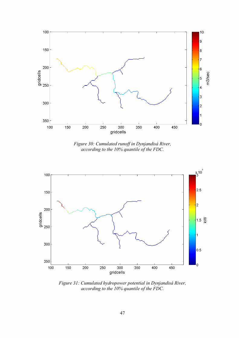
47
Figure 30: Cumulated runoff in Dynjandisá River, according to the 10% quantile of the FDC.
Figure 31: Cumulated hydropower potential in Dynjandisá River, according to the 10% quantile of the FDC.

Figure 32: Results of the estimated technical hydropower potential for the Dynjandisá River, according to the 10% quantile of the FDC. The two domains marked with number 1 and 2 represent the outlines of two other maps, presented in Appendix II.
48

49
Summary of Hydropower potential estimations for Dynjandisá River Mean runoff and six different quantiles of the FDC have been used to estimate hydropower potential according to eq. (1). This gives seven different results of technical hydropower potential for the catchment of Dynjandisá River. By analyzing the maps in Section 4.1.2, it can be seen that the highest potential is in all cases located at the waterfalls in Dynjandisá River for which the head is highest. The sections of the river that carry hydropower potential is the same between the different quantiles, as expected, the only difference is that with lower quantiles of the FDC (more discharge), the number of river cells with hydropower potential increases. This shows that visual presentation on maps is not necessary for all of the quantiles.
Table 18 gives comparison of the different quantiles as it summarizes the resulting number of cells within specified range of hydropower values as well as the total cumulated hydropower potential. The upper values in the table show number of cells within the range of defined values of hydropower potential, given different quantiles of the FDC for simulated runoff. The lower values show the proportion of the upper value to the total number of river cells. It is noted that the 10% quantile of the FDC gives the highest discharge estimation and therefore the highest value of total hydropower potential. The mean runoff in Dynjandisá River corresponds to the 35% quantile of the FDC and gives therefore the second highest hydropower potential, then the 50% and so on. The 95% quantile of the FDC gives an estimation of the extreme low flow and the lowest estimation of hydropower potential is therefore assuming the 95% quantile of the FDC.
The results of total power, calculated with the routed runoff, vary from 3,535 kW given 95% FDC to 30,359 kW given 10% FDC. This wide range in results can be expected since these calculations are based on extreme high-flows and low-flows in a direct-runoff river over a 10 year period. Assuming that the mean runoff would be used in storage hydropower projects, the total available power would be 13,575 kW. For a run-of-river hydropower projects, using 75% FDC, the total available hydropower would be 4,372 kW. The portion of the total power, originating from low power, differs between quantiles. The largest portion of low power cells is logically connected to the lowest discharge where 37% of the total power originates from river cells with less than 30 kW hydropower potential, assuming 95% or 85% quantile of the FDC. Only 6% of the total cumulated hydropower potential, assuming the 10% quantile of the FDC, originates from such low power river cells.
Figure 33 shows also the comparison of results, given different quantiles of the FDC, with an overview of the river cells carrying hydropower potential. The x-axis shows percentage of the total number of river cells in the catchment and the y-axis shows the hydropower potential in kW for each river cell. The figure shows the percentage of river cells carrying particular hydropower potential or more. This shows that less than 16% of the total number of river cells has some hydropower potential.

50
Table 18: Comparison of the amount of river cells within specified range of hydropower values and the total cumulated hydropower potential, given different quantiles of the FDC.
Power (kW) 0-10 10-30 30-50 50-100 100-1000 1000-5000 Total Power
Mean runoff 146 6.9%
95 4.5%
26 1.2%
26 1.2%
33 1.6%
0 0% 13,575
95% FDC 260 12.2
35 1.6%
12 0.6%
13 0.6%
6 0.3%
0 0% 3,535
85% FDC 256 12.0
39 1.8%
11 0.5%
13 0.6%
7 0.3%
0 0% 3,991
75% FDC 248 11.7
43 2.0%
13 0.6%
14 0.7%
8 0.4%
0 0% 4,372
65% FDC 241 11.3
46 2.2%
15 0.7%
15 0.7%
9 0.4%
0 0% 4,984
50% FDC 196 9.2%
81 3.8%
14 0.7%
15 0.7%
20 0.9%
0 0% 7,273
10% FDC 87 4.1%
75 3.5%
46 2.2%
52 2.4%
62 2.9%
4 0.2% 30,359
Figure 33: Distribution of potential hydropower per river cell for different quantiles of the FDC. The mean runoff corresponds to the 35% FDC.
0
100
200
300
400
500
600
700
800
0% 2% 4% 6% 8% 10% 12% 14% 16%
Pow
er [k
W]
Percentage of river cells
50% FDC65% FDC75% FDC85% FDC95% FDCMean runoff10% FDC
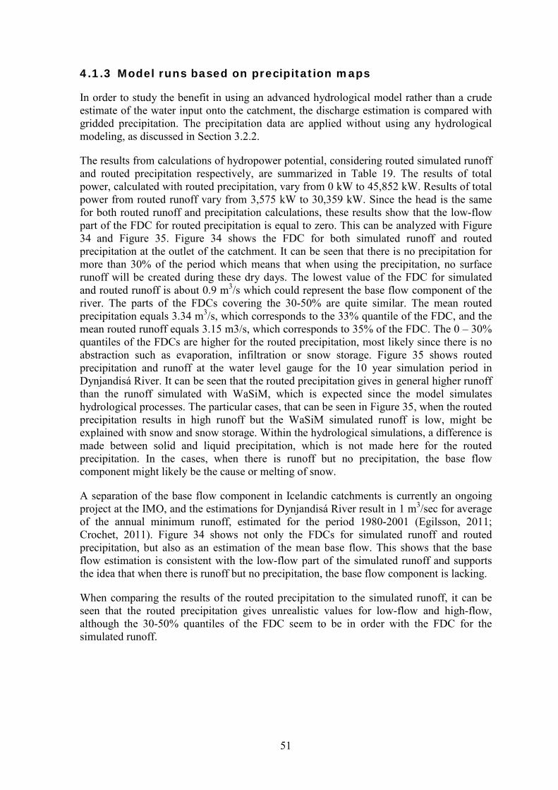
51
4.1.3 Model runs based on precipitation maps
In order to study the benefit in using an advanced hydrological model rather than a crude estimate of the water input onto the catchment, the discharge estimation is compared with gridded precipitation. The precipitation data are applied without using any hydrological modeling, as discussed in Section 3.2.2.
The results from calculations of hydropower potential, considering routed simulated runoff and routed precipitation respectively, are summarized in Table 19. The results of total power, calculated with routed precipitation, vary from 0 kW to 45,852 kW. Results of total power from routed runoff vary from 3,575 kW to 30,359 kW. Since the head is the same for both routed runoff and precipitation calculations, these results show that the low-flow part of the FDC for routed precipitation is equal to zero. This can be analyzed with Figure 34 and Figure 35. Figure 34 shows the FDC for both simulated runoff and routed precipitation at the outlet of the catchment. It can be seen that there is no precipitation for more than 30% of the period which means that when using the precipitation, no surface runoff will be created during these dry days. The lowest value of the FDC for simulated and routed runoff is about 0.9 m3/s which could represent the base flow component of the river. The parts of the FDCs covering the 30-50% are quite similar. The mean routed precipitation equals 3.34 m3/s, which corresponds to the 33% quantile of the FDC, and the mean routed runoff equals 3.15 m3/s, which corresponds to 35% of the FDC. The 0 – 30% quantiles of the FDCs are higher for the routed precipitation, most likely since there is no abstraction such as evaporation, infiltration or snow storage. Figure 35 shows routed precipitation and runoff at the water level gauge for the 10 year simulation period in Dynjandisá River. It can be seen that the routed precipitation gives in general higher runoff than the runoff simulated with WaSiM, which is expected since the model simulates hydrological processes. The particular cases, that can be seen in Figure 35, when the routed precipitation results in high runoff but the WaSiM simulated runoff is low, might be explained with snow and snow storage. Within the hydrological simulations, a difference is made between solid and liquid precipitation, which is not made here for the routed precipitation. In the cases, when there is runoff but no precipitation, the base flow component might likely be the cause or melting of snow.
A separation of the base flow component in Icelandic catchments is currently an ongoing project at the IMO, and the estimations for Dynjandisá River result in 1 m3/sec for average of the annual minimum runoff, estimated for the period 1980-2001 (Egilsson, 2011; Crochet, 2011). Figure 34 shows not only the FDCs for simulated runoff and routed precipitation, but also as an estimation of the mean base flow. This shows that the base flow estimation is consistent with the low-flow part of the simulated runoff and supports the idea that when there is runoff but no precipitation, the base flow component is lacking.
When comparing the results of the routed precipitation to the simulated runoff, it can be seen that the routed precipitation gives unrealistic values for low-flow and high-flow, although the 30-50% quantiles of the FDC seem to be in order with the FDC for the simulated runoff.
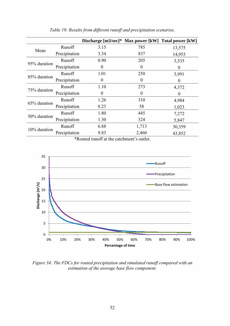
52
Table 19: Results from different runoff and precipitation scenarios.
Discharge [m3/sec]* Max power [kW] Total power [kW]
Mean Runoff 3.15 785 13,575
Precipitation 3.34 837 14,953
95% duration Runoff 0.90 205 3,535
Precipitation 0 0 0
85% duration Runoff 1.01 250 3,991
Precipitation 0 0 0
75% duration Runoff 1.10 273 4,372
Precipitation 0 0 0
65% duration Runoff 1.26 310 4,984
Precipitation 0.23 58 1,023
50% duration Runoff 1.80 445 7,272
Precipitation 1.30 324 5,847
10% duration Runoff 6.88 1,713 30,359
Precipitation 9.83 2,460 43,852 *Routed runoff at the catchment’s outlet.
Figure 34: The FDCs for routed precipitation and simulated runoff compared with an estimation of the average base flow component.
0
5
10
15
20
25
30
35
0% 10% 20% 30% 40% 50% 60% 70% 80% 90% 100%
Disc
harg
e (m
ᶟ/s)
Percentage of time
Runoff
Precipitation
Base flow estimation

53
Figure 35: Routed precipitation and runoff at the water level gauge in Dynjandisá River.
0
5
10
15
20
25
30
0 5 10 15 20 25 30
Rout
ed to
tal r
unof
f (mᶟ/
sec)
Routed precipitation (mᶟ/sec)

54
4.2 Sandá River in Þistilfjörður Sandá River in Þistilfjörður is located in the northeast of Iceland and has an area of 268 km2 (Icelandic Meteorological Office, 2011b). The location of the catchment can be seen in Figure 36. The Sandá River is a direct runoff river with a considerable springfed contribution (Icelandic Meteorological Office, 2011b). Discharge rating curves, corresponding to the water-level gauge in Sandá River are available from the beginning of continuous measurements in 1965 but also from some earlier measurements from 1944 when a potential hydropower plant was planned.
Figure 36: Location of the catchment of Sandá River.
Table 20 shows a comparison of observed and simulated discharge at the water level gauge for the simulation period 1992-2001. The table also shows observed discharge for a longer discharge serie from 1966 to 2004. It can be seen that the observed discharge serie for the simulation period should give a sufficient estimation of the long-run mean discharge for Sandá River. The maximum daily discharge is the same for both periods and the minimum similar. For the simulated discharge, the table shows that the mean discharge is too low compared to the observed discharge. The minimum and maximum daily simulated discharge is also lower than the observed ones. Since the simulation period seems to give sufficient estimation of the longer discharge serie, this difference could be due to the fact that the WaSiM simulations for this catchment were performed without using newest improvements and data in high resolution.
Figure 37 shows the flow duration curve (FDC) for Sandá River, according to simulated discharge at the outlet of the catchment. The FDC is similar to the FDC for Dynjandisá River (Figure 9) which is normal since they are both direct runoff rivers. The mean simulated discharge corresponds to the 25% quantile of the FDC for the same period, which means that for 25% of the simulation period, 11.3 m3/s are equaled or exceeded.

55
Table 20: Comparison of observed and simulated discharge at the water level gauge in Sandá River.
Mean daily discharge (mᶟ/s)
Observations Simulations
1966-2004 1992-2001 1992-2001 mean 13.2 13.5 11.3 min 2.6 2.7 2.3 max 121 121 108.3
Figure 37: A FDC for Sandá River (vhm 26), the discharge is simulated at the water level gauge, close to the catchment’s outlet, over the simulation period.
0
20
40
60
80
100
120
0% 20% 40% 60% 80% 100%
Disc
harg
e (m
ᶟ/s)
Percentage of time

56
4.2.1 Head
The head grid shows elevation difference between river cells along the channel. For Sandá River, the maximum elevation difference between two consecutive river cells are 17 m and the cumulated head along the river network is 5328 m. Difference between the lowest and the highest point is 986 m according to the digital elevation map but since the cumulated head accumulates elevation difference between cells along the total river network covering all tributaries, the cumulated head is much higher. Figure 38 shows the elevation difference between two consecutive river cells along the river network of Sandá River. The head values are divided into three ranges; 1-3 m head is illustrated with green dots, 4-10 m with yellow dots and 11-17 m with red dots. The figure illustrates that the head cumulates steadily, as the majority of the river network has some elevation difference between two consecutive river cells, in most cases 1-3 m. This shows that most of the river network will have some hydropower potential as long as the discharge is available.

57
Figure 38: The head grid for Sandá River presented on a map.

58
4.2.2 Hydropower potential
The results for Sandá River are presented on two different maps. The first one representing the mean runoff which can be used to estimate the hydropower potential assuming storage projects, using reservoir to regulate the water. The second one represents low flow where the 75% quantile is used in order to estimate the potential assuming run-of-river projects. One extra Section is made, Hydropower potential given different quantiles of the FDC, to analyze results of hydropower calculations assuming other quantiles of the FDC, as discussed in Section 3.3. The runoff data used in calculations for the catchment is provided without recent improvements in WaSiM, as discussed in the beginning of Chapter 4.
Hydropower potential given mean runoff The mean runoff for the 10 year simulation period is 11.3 m3/s, simulated at the water level gauge, close to the outlet of the catchment. The hydropower calculations assuming mean runoff result in a total hydropower of 44,714 kW where the maximum power value is calculated 1,283 kW per single cell. Table 21 shows the total resulting power, cumulated along the river network. The last two columns give the results of total cumulated power where river cells resulting in less than 10 kW and 30 kW are excluded. If all river cells resulting in hydropower potential less than 10 kW are excluded, the result will show about 7% less than the total cumulated power for all the river cells. If river cells resulting in less than 30 kW are excluded, the result will about 13% less than the original value of cumulated power. This illustrates that up to 13% of the total cumulated power, estimated assuming mean runoff, originates from river cells with such low power that it may in some cases be difficult to utilize.
Table 22 presents the number of river cells resulting in specific range of power, assuming mean runoff. Most of the river cells have potential hydropower in the range of 1-10 kW and only one river cell has more than 1000 kW as potential hydropower. This is also presented in Figure 39, where the location of power per cell, the location of the water-level gauge and the outlines of the catchment are presented on a map. It can be seen that the bulkier part of the river network results in some hydropower potential. The tributaries are largely covered with green and light green dots which represent 10-50 kW hydropower potential for every river cell, while the main channel, downstream of the main tributaries, has mostly yellow and orange dots which represent hydropower potential from 50 kW to 1000 kW.
Table 21: The total resulting hydropower potential in Sandá River, assuming mean runoff.
All cells < 10 kW excluded < 30 kW excluded
Total power [kW] 44,714 41,672 38,730
Table 22: The number of cells within the range of defined values of hydropower potential calculated with mean runoff.
Power (kW) 0-10 10-30 30-50 50-100 100-1000 1000-5000
Cell (number) 2008 167 47 151 117 1
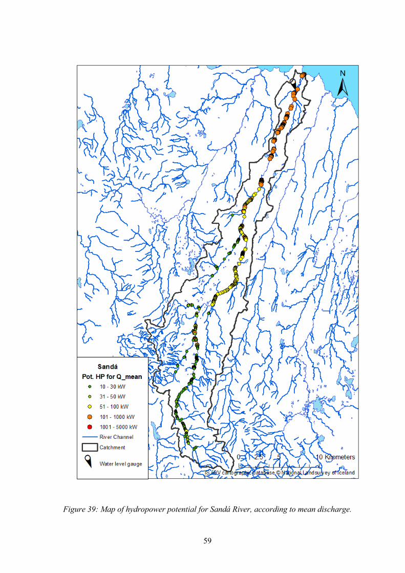
59
Figure 39: Map of hydropower potential for Sandá River, according to mean discharge.

60
Hydropower potential given 75% FDC The 75% quantile of the FDC is chosen to represent the low flow which is used for the estimation of hydropower potential assuming run-of-river projects. The 75% quantile for the 10 year simulation period is 5.27 m3/sec simulated at the water level gauge, close to the outlet of the catchment. This hydropower calculations assuming the 75% quantile result in total hydropower of 20,226 kW where the maximum power value is calculated 593 kW per single cell. Table 23 shows the total resulting power, cumulated along the river network. The last two columns give the results of total cumulated power where river cells resulting in less than 10 kW and 30 kW are excluded. If all river cells resulting in hydropower potential less than 10 kW are excluded, the result will show about 7% less than the total cumulated power for all the river cells. When river cells resulting in less than 30 kW are excluded, the result will be about 16% less than the original value of cumulated power. This illustrates that up to 16% of the total cumulated power, estimated assuming mean runoff, originates from river cells with such low power that it may in some cases be difficult to utilize.
Table 24 presents the number of river cells resulting in specific range of power, assuming the 75% quantile of the FDC. Most of the river cells have potential hydropower in the range of 1-10 kW and since the maximum power value is calculated 593 kW, no cell has more than 1000 kW as potential hydropower. This is also presented in Figure 40, where the location of power per cell, the location of the water-level gauge and the outlines of the catchment are presented on a map. It can be seen that the bulkier part of the river network still results in some hydropower potential as for the potential hydropower given mean runoff. The figure shows that a large part of the main channel has now green and light green dots which represent 10-50 kW.
Table 23: The total resulting hydropower potential in Sandá River, assuming the 75% quantile of the FDC.
All cells < 10 kW excluded < 30 kW excluded
Total power [kW] 20,226 18,808 16,976
Table 24: The number of cells within the range of defined values of hydropower potential calculated with 75% FDC.
Power (kW) 0-10 10-30 30-50 50-100 100-1000 1000-5000
Cell (number) 2,110 110 189 37 34 0

61
Figure 40: Map of hydropower potential for Sandá River, according to 75% FDC.

62
Hydropower potential given different quantiles of the FDC Results of the calculations for Sandá River are only mapped assuming mean discharge and the 75% quantile of the FDC, but Table 25 gives comparison of the results assuming the different quantiles as discussed in Section 3.3. The table summarizes the resulting number of cells within specified range of hydropower values as well as the total cumulated hydropower potential. The upper values in the table show number of cells within the range of defined values of hydropower potential, given different quantiles of the FDC for simulated runoff. The lower values show the proportion of the upper value to the total number of river cells. It is noted that the 10% quantile of the FDC gives the highest discharge estimation and therefore the highest value of total hydropower potential. The mean runoff corresponds to the 25% quantile of the FDC and gives therefore the second highest hydropower potential, then the 50% and so on. The 95% quantile of the FDC gives an estimation of the extreme low flow and the lowest estimation of hydropower potential is therefore assuming the 95% quantile of the FDC.
The results of total power, calculated with the routed runoff, vary from 15,945 kW given 95% FDC to 96,787 kW given 10% FDC. This wide range in results can be expected since these calculations are based on extreme high-flows and low-flows over a 10 year period. Assuming that the mean runoff would be used in a storage hydropower project, the total available power would be 44,714 kW. For a run-of-river hydropower project, using 75% FDC, the total available hydropower would be 20,226 kW.
Table 25: Comparison of the amount of river cells within specified range of hydropower values and the total cumulated hydropower potential, given different quantiles of the FDC.
Power (kW) 0-10 10-30 30-50 50-100 100-1000 1000-5000 Total
Mean runoff 2008 28.1%
167 2.3%
47 0.7%
151 2.1%
117 1.6%
1 0.0% 44,714
95% FDC 2051 28.7%
170 2.4%
120 1.7%
27 0.4%
30 0.4%
0 0.0% 15,945
85% FDC 2110 29.5%
123 1.7%
182 2.5%
26 0.4%
31 0.4%
0 0.0% 18,853
75% FDC 2110 29.5%
110 1.5%
189 2.6%
37 0.5%
34 0.5%
0 0.0% 20,226
65% FDC 2103 29.5%
115 1.6%
145 2.0%
75 1.1%
43 0.6%
0 0.0% 21,791
50% FDC 2096 29.4%
126 1.7%
107 1.5%
110 1.5%
48 0.7%
0 0.0% 24,662
10% FDC 2008 28.1%
226 3.2%
83 1.2%
66 0.9%
265 3.7%
8 0.1% 96,787

63
4.2.3 Model runs based on precipitation maps
In order to study the benefit in using an advanced hydrological model rather than a crude estimate of the water input onto the catchment, the discharge estimation is compared with gridded precipitation. The precipitation data are applied without using any hydrological modeling, as discussed in Section 3.2.2.
The results from calculations of hydropower potential, considering routed simulated runoff and routed precipitation respectively, are summarized in Table 26. The results of total hydropower, calculated with routed precipitation, vary from 0 kW to 152,700 kW. Results of total hydropower from routed runoff vary from 15,945 kW to 96,787 kW. These results indicate that the low-flow part of the FDC for routed precipitation is equal to zero. This can be analysed with Figure 41, which shows the FDC at the water level gauge, for both simulated runoff and routed precipitation. It can be seen that there is no precipitation for 40% of the period which means that when using the precipitation, no surface runoff will be created during these dry days. The lowest value of the FDC for routed runoff is about 3.8 m3/s which could represent the base flow component of the river. The parts of the FDCs covering the 30-50% are quite similar. The mean routed precipitation equals 13.66 m3/s, which corresponds to the 31% quantile of the FDC for routed precipitation.The mean simulated and routed runoff equals 11.34 m3/s, which corresponds to 25% of the FDC. The 0-40% quantiles of the FDCs are higher for the routed precipitation, most likely since there is no abstraction such as evaporation, infiltration or snow storage.
Figure 41 shows not only the FDCs for routed precipitation and runoff, but also an estimation of the mean base flow. The base flow component for Sandá River, results in ca. 5.7 m3/sec for average of the annual minimum runoff, estimated for the period 1965-2003 (Egilsson, 2011; Crochet, 2011). Figure 41 shows that the base flow estimation is consistent with the low-flow part of the simulated runoff. This supports the idea that when there is runoff but no precipitation, the base flow component is lacking. This could though also be due to snowmelt. When comparing the results of the routed precipitation to the simulated runoff, it can be seen that the results are the same as for Dynjandisá River; routed precipitation gives unrealistic values for low-flow and high-flow, although the 30-50% quantiles of the FDC seem to be in order with the FDC for the simulated runoff.

64
Table 26: Results from different runoff and precipitation scenarios.
Discharge [m3/sec]* Max power [kW] Total power [kW]
Mean Runoff 11.34 1283 44,714
Precipitation 13.66 1538 55,425
95% duration Runoff 3.86 445 15,945
Precipitation 0 0 0
85% duration Runoff 4.90 551 18,853
Precipitation 0 0 0
75% duration Runoff 5.27 593 20,226
Precipitation 0 0 0
65% duration Runoff 5.71 640 21,791
Precipitation 0.37 34 810
50% duration Runoff 6.52 724 24,662
Precipitation 5.06 573 21,414
10% duration Runoff 25.42 2869 96,787
Precipitation 37.52 4237 152,700 *Routed runoff at the catchment’s outlet.
Figure 41: The FDCs for routed precipitation and runoff and an estimation of the average base flow component.
0
20
40
60
80
100
120
140
160
180
200
0% 20% 40% 60% 80% 100%
Disc
harg
e (m
ᶟ/s)
Percentage of time
Runoff
Precipitation
Baseflow estimation

65
4.3 Austari-Jökulsá River The catchment of Austari-Jökulsá River is situated in the central highland and has an area of 1200 km2 (Rist, 1990). The location of the catchment can be seen in Figure 42. The catchment is highly elevated for an Icelandic catchment and has 10% glacier coverage (Rist, 1990). The Austari-Jökulsá River is mainly spring-fed but has also characteristics of a direct run-off river and of a glacier river (Icelandic Meteorological Office, 2011c). Discharge rating curves, corresponding to a water-level gauge in Austari-Jökulsá River are available from 1971.
Figure 42: Location of the catchment of Austari-Jökulsá River.
Table 27 shows a comparison of observed and simulated discharge at the water level gauge as well as a comparison of observed discharge for the simulation period 1992-2001 and for a longer discharge serie from 1972 to 2004. The table shows that although the observed maximum and minimum daily discharge is the same for both the simulation period and for the longer discharge serie, the mean discharge is not the same. It is therefore possible that the observed discharge serie for the simulation period does not give a sufficient estimation of the long-run mean discharge for Sandá River. For the simulated discharge, the table shows that the mean discharge is too low compared to the observed discharge. The minimum and maximum daily simulated discharge is also lower than the observed ones. This difference could be due to the chosen simulation period, or due to the fact that the WaSiM simulations for this catchment were performed without using newest improvements and data in high resolution. This will not be changed at this point since the same simulation period was chosen for all three catchments at the beginning of the study.
Figure 43 shows the flow duration curve (FDC) for the river, according to simulated discharge at the water level gauge, close to the outlet of the catchment. The mean simulated discharge corresponds to the 33% quantile of the FDC for the same period, which means that for 33% of the simulation period, 31.7 m3/s are equaled or exceeded.
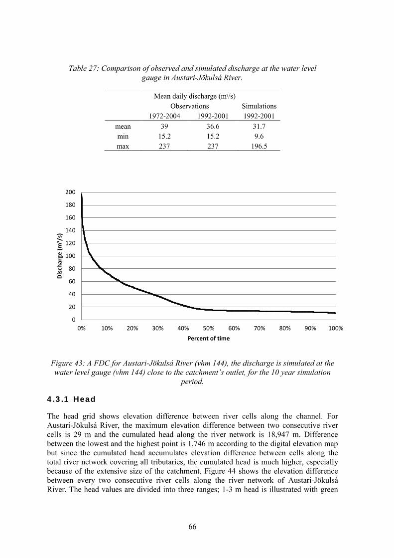
66
Table 27: Comparison of observed and simulated discharge at the water level gauge in Austari-Jökulsá River.
Mean daily discharge (mᶟ/s)
Observations Simulations
1972-2004 1992-2001 1992-2001 mean 39 36.6 31.7 min 15.2 15.2 9.6 max 237 237 196.5
Figure 43: A FDC for Austari-Jökulsá River (vhm 144), the discharge is simulated at the water level gauge (vhm 144) close to the catchment’s outlet, for the 10 year simulation
period.
4.3.1 Head
The head grid shows elevation difference between river cells along the channel. For Austari-Jökulsá River, the maximum elevation difference between two consecutive river cells is 29 m and the cumulated head along the river network is 18,947 m. Difference between the lowest and the highest point is 1,746 m according to the digital elevation map but since the cumulated head accumulates elevation difference between cells along the total river network covering all tributaries, the cumulated head is much higher, especially because of the extensive size of the catchment. Figure 44 shows the elevation difference between every two consecutive river cells along the river network of Austari-Jökulsá River. The head values are divided into three ranges; 1-3 m head is illustrated with green
0
20
40
60
80
100
120
140
160
180
200
0% 10% 20% 30% 40% 50% 60% 70% 80% 90% 100%
Disc
harg
e (m
ᶟ/s)
Percent of time

67
dots, 4-10 m with yellow dots and 11-29 m with red dots. Figure 44 illustrates that the head cumulates steadily, as the majority of the river network has some elevation difference between two consecutive river cells, in most cases 1-3 m. This shows that most of the river network will have some hydropower potential as long as the discharge is available. The tributaries of the river could have high hydropower potential since most of the red dots are located in the tributaries.

68
Figure 44: The head grid for Austari-Jökulsá River presented on a map.

69
4.3.2 Hydropower potential
The results for Austari-Jökulsá River are presented on two different maps as for the results of Sandá River. The first one represents hydropower potential assuming mean runoff, which can be used to estimate and locate the hydropower potential for storage projects using reservoir to regulate the water. The second one represents hydropower potential assuming low flow, where the 75% quantile of the FDC is used in order to estimate the potential for run-of-river projects. One extra Section is made, Hydropower potential given different quantiles of the FDC, to analyze results of hydropower calculations assuming other quantiles of the FDC, as discussed in Section 3.3. The runoff data used in calculations for the catchment are provided without recent improvements in WaSiM, as discussed in the beginning of Chapter 4.
Hydropower potential given mean runoff The mean runoff for the 10 year simulation period is 31,7 m3/sec, simulated at the water level gauge, close to the outlet of the catchment. The hydropower calculations for Austari-Jökulsá River, assuming mean runoff, result in a total hydropower of 281,270 kW. The maximum hydropower potential is calculated 5,592 kW per single cell.
Table 28 shows the total resulting power, cumulated along the river network. The last two columns give the results of total cumulated power where river cells resulting in less than 10 kW and 30 kW are excluded. If all river cells resulting in hydropower potential less than 10 kW are excluded, the result will show about 4% less than the total cumulated power for all the river cells. When river cells resulting in less than 30 kW are excluded, the result will show about 10% less than the original value of cumulated power. This implies that up to 10% of the total cumulated power, estimated assuming mean runoff, originates from river cells with such low power that it may in some cases be difficult to utilize.
Table 29 presents the number of river cells resulting in specific range of power, assuming mean runoff. Most of the river cells have potential hydropower in the range of 1-10 kW and only one river cell has more than 5000 kW as potential hydropower. This is also presented in Figure 45, where the location of power per cell, the location of the water-level gauge and the outlines of the catchment are presented on a map. It can be seen that the bulkier part of the river network results in some hydropower potential. The tributaries are largely covered with green and light green dots which represent 10-50 kW hydropower potential for every river cell, while the main stream is mostly covered with yellow and orange cells representing 51-1000 kW hydropower potential.
70
Table 28: The total resulting hydropower potential in Austari-Jökulsá River, assuming mean runoff.
All cells < 10 kW excluded < 30 kW excluded
Total power [kW] 281,270 270,870 255,170
Table 29: The number of cells within the range of defined values of hydropower potential calculated with mean runoff.
Power (kW) 0-10 10-30 30-50 50-100 100-1000 1000-5000 > 5000
Cell (number) 5,871 954 275 90 587 27 1

71
Figure 45: Map of hydropower potential for Austari-Jökulsá River, according to mean discharge.

72
Hydropower potential given 75% FDC The 75% quantile of the FDC is chosen to represent the low flow which is used for the estimation of hydropower potential for run-of-river projects. The 75% quantile for the 10 year simulation period is 13.3 m3/sec simulated at a water level gauge, close to the outlet of the catchment. This quantile results in total power of 103,020 kW where the maximum hydropower potential is calculated 2,344 kW per single cell.
Table 30 shows the total resulting power, cumulated along the river network. The last two columns give the results of total cumulated power where river cells resulting in less than 10 kW and 30 kW are excluded. If all river cells resulting in hydropower potential less than 10 kW are excluded, the result will show about 6% less than the total cumulated power for all the river cells. When river cells resulting in less than 30 kW are excluded, the result will show about 12% less than the original value of cumulated power. This illustrates that up to 12% of the total cumulated power, estimated assuming mean runoff, originates from low power river cells which may in some cases be difficult to utilize.
Table 31 presents the number of river cells resulting in specific range of power, assuming the 75% quantile of the FDC. Most of the river cells have potential hydropower in the range of 1-10 kW and since the maximum power value is calculated 2,344 kW, no cell has more than 5000 kW as potential hydropower. These results are also presented in Figure 46, where the location of power per cell, the location of the water-level gauge and the outlines of the catchment are presented on a map. It can be seen that the bulkier part of the river network still results in some hydropower potential as for the potential hydropower given mean runoff. The tributaries do not have hydropower potential as far upstream as for the hydropower potential given mean runoff, but the river cells that do result in hydropower potential are mostly representing 10-50 kW (green and light green). The main stream goes from yellow to orange colored river cells upstream to downstream, representing 51-2,344 kW which is the maximum power value per single cell.
Table 30: The total resulting hydropower potential in Austari-Jökulsá River, assuming the 75% quantile of the FDC.
All cells < 10 kW excluded < 30 kW excluded
Total power [kW] 103,020 96,474 90,646
Table 31: The number of cells within the range of defined values of hydropower potential calculated with 75% FDC.
Power (kW) 0-10 10-30 30-50 50-100 100-1000 1000-5000 > 5000
Cell (number) 5731 382 34 188 345 9 0

73
Figure 46: Map of hydropower potential for Austari-Jökulsá River, according to 75% quantile of the FDC.
74
Hydropower potential given different quantiles of the FDC Results of the calculations for Austari-Jökulsá River are only mapped assuming mean discharge and the 75% quantile of the FDC as for the results of Sandá river.Table 32 gives comparison of the different quantiles discussed in Section 3.3. The table summarizes the resulting number of cells within specified range of hydropower values as well as the total cumulated hydropower potential. The upper values in the table show number of cells within the range of defined values of hydropower potential, given different quantiles of the FDC for simulated runoff. The lower values show the proportion of the upper value to the total number of river cells. It is noted that the 10% quantile of the FDC gives the highest discharge estimation and therefore the highest value of total hydropower potential. The mean runoff corresponds to the 33% quantile of the FDC and gives therefore the second highest hydropower potential, then the 50% and so on. The 95% quantile of the FDC gives an estimation of the extreme low flow and the lowest estimation of hydropower potential is therefore assuming the 95% quantile of the FDC.
The results of total power, calculated with the routed runoff, vary from 87,918 kW given 95% FDC to 680,700 kW given 10% FDC. Assuming that the mean runoff would be used in a storage hydropower project, the total available power would be 281,270 kW. For a run-of-river hydropower project, using 75% FDC, the total available hydropower would be 103,020 kW.
Table 32: Comparison of the amount of river cells within specified range of hydropower values and the total cumulated hydropower potential, given different quantiles of the FDC.
Power (kW) 0-10 10-30 30-50 50-100 100-1000 1000-5000 > 5000 Total
Mean runoff
5871 13.4%
954 2.2%
275 0.6%
90 0.2%
587 1.3%
27 0.1%
1 0.0% 281,270
95% FDC 3394 7.8%
296 0.7%
22 0.1%
349 0.8%
184 0.4%
7 0.0%
0 0.0% 87,918
85% FDC 4765 84.1%
335 7.7%
26 0.1%
253 0.6%
282 0.6%
7 0.0%
0 0.0% 96,322
75% FDC 5731 10.9%
382 0.8%
34 0.1%
188 0.4%
345 0.8%
9 0.0%
0 0.0% 103,020
65% FDC 5997 13.7%
403 5.8%
40 0.1%
172 0.4%
361 0.8%
9 0.0%
0 0.0% 107,500
50% FDC 6175 14.1%
443 0.9%
44 0.1%
57 0.1%
473 1.1%
13 0.0%
0 0.0% 119,300
10% FDC 5054 11.6%
1194 2.7%
371 0.8%
325 0.7%
757 1.7%
94 0.2%
10 0.0% 680,700
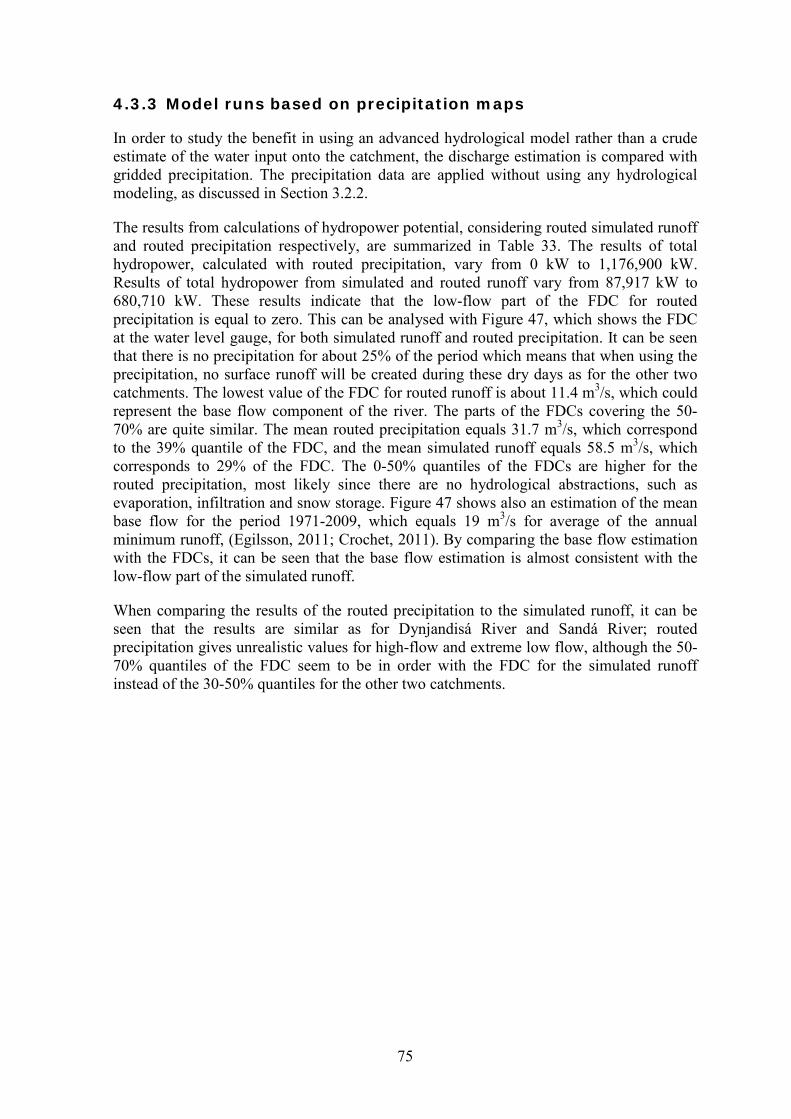
75
4.3.3 Model runs based on precipitation maps
In order to study the benefit in using an advanced hydrological model rather than a crude estimate of the water input onto the catchment, the discharge estimation is compared with gridded precipitation. The precipitation data are applied without using any hydrological modeling, as discussed in Section 3.2.2.
The results from calculations of hydropower potential, considering routed simulated runoff and routed precipitation respectively, are summarized in Table 33. The results of total hydropower, calculated with routed precipitation, vary from 0 kW to 1,176,900 kW. Results of total hydropower from simulated and routed runoff vary from 87,917 kW to 680,710 kW. These results indicate that the low-flow part of the FDC for routed precipitation is equal to zero. This can be analysed with Figure 47, which shows the FDC at the water level gauge, for both simulated runoff and routed precipitation. It can be seen that there is no precipitation for about 25% of the period which means that when using the precipitation, no surface runoff will be created during these dry days as for the other two catchments. The lowest value of the FDC for routed runoff is about 11.4 m3/s, which could represent the base flow component of the river. The parts of the FDCs covering the 50-70% are quite similar. The mean routed precipitation equals 31.7 m3/s, which correspond to the 39% quantile of the FDC, and the mean simulated runoff equals 58.5 m3/s, which corresponds to 29% of the FDC. The 0-50% quantiles of the FDCs are higher for the routed precipitation, most likely since there are no hydrological abstractions, such as evaporation, infiltration and snow storage. Figure 47 shows also an estimation of the mean base flow for the period 1971-2009, which equals 19 m3/s for average of the annual minimum runoff, (Egilsson, 2011; Crochet, 2011). By comparing the base flow estimation with the FDCs, it can be seen that the base flow estimation is almost consistent with the low-flow part of the simulated runoff.
When comparing the results of the routed precipitation to the simulated runoff, it can be seen that the results are similar as for Dynjandisá River and Sandá River; routed precipitation gives unrealistic values for high-flow and extreme low flow, although the 50-70% quantiles of the FDC seem to be in order with the FDC for the simulated runoff instead of the 30-50% quantiles for the other two catchments.

76
Table 33: Results from different runoff and precipitation scenarios.
Discharge [m3/sec]* Max power [kW] Total power [kW]
Mean Runoff 31.7
5,592 281,270 Precipitation 58.5 10,320 523,400
95% duration Runoff 11.4 2,017 87,917
Precipitation 0 0 0
85% duration Runoff 12.5 2,204 96,322
Precipitation 0 0 0
75% duration Runoff 13.3 2,344 103,020
Precipitation 1.2 211 5,499
65% duration Runoff 13.7 2,420 107,500
Precipitation 7.9 1,400 55,803
50% duration Runoff 15.4 2,721 119,300
Precipitation 24.8 4,378 213,110
10% duration Runoff 72.8 12,849 680,710
Precipitation 129.7 22,899 1,176,900 *Routed runoff at the catchment’s outlet.
Figure 47: The FDCs for routed precipitation and runoff and an estimation of the average base flow component in Austari-Jökulsá River.
0
50
100
150
200
250
300
350
400
0% 20% 40% 60% 80% 100%
Disc
harg
e (m
ᶟ/s)
Percentage of time
Runoff
Precipitation
Baseflow estimation
77
4.4 Summary and comparison The method described in Chapter 3 was applied to three catchments; Dynjandisá River, Sandá River and Austari-Jökulsá River. The catchments are different in both size and location, but the discharge characteristics are partly similar. Dynjandisá River and Sandá River are both direct-runoff rivers (Rist, 1990) although the discharge in Dynjandisá River is mitigated by small lakes and Sandá River has a substantial spring-fed contribution. Austari-Jökulsá River is mainly spring-fed but has also some characteristics of a direct-runoff river and of a glacier river (Rist, 1990). Figure 48 shows the ratio of simulated daily runoff and the mean runoff over the 10 year simulation period for each river. It can be seen that the rivers have similar discharge characteristics in terms of the FDCs. Figure 49 shows that the discharge characteristics in terms of quantity or volume of discharge is quite different between rivers. The difference is mainly due to the different size of the catchments.
The distribution of available head along the three river networks differs. Most of the elevation difference is in the downstream part of the Dynjandisá River, close to the water level gauge, while the upstream part of the Sandá River has more elevation difference than the downstream one. The catchment of Austari-Jökulsá River has almost constant elevation difference from source to river outlet.
The results show that all of the catchments have possibilities regarding technical hydropower potential. The magnitude of potential hydropower is though not comparable because of the different catchment size and therefore different volume of discharge as shown in Figure 49. The location of the hydropower potential is connected to the distribution of available head where most of the potential hydropower in Dynjandisá River is located downstream in the catchment, upstream in Sandá River and almost evenly distributed in Austari-Jökulsá River, according to the maps in Sections 4.1-4.3. This connection between the location of available head and potential hydropower shows that mapping of results assuming numerous different quantiles of the FDC are unnecessary. The 75% quantile and the mean flow, used for mapping the potential hydropower in Sandá River and Austari-Jökulsá River, should therefore be sufficient. The portion of river cells with technical hydropower potential is also different between catchments where 16-18% of the river cells in Dynjandisá River and Austari-Jökulsá River have hydropower potential, but more than 33% of the river cells in Sandá River.
It is interesting to see the different portion of the base flow component between the catchments The base flow component in Dynjandisá River corresponds to the 85% quantile of the FDC while base flow in Sandá River corresponds to the 65% quantile and in Austari-Jökulsá River to the 50% quantile of the FDC. Since the base flow is often used to represent the minimal volume of water required for the river to maintain ecological balance, e.g. in terms of habitats (Department of the Environment, Climate change, Energy and Water, 2009), this high proportion of base flow in Sandá River and Austari-Jökulsá River could have profound effect on the exploitable hydropower potential. It is though noted that estimating the quantile of the FDC corresponding to the base flow component for Austari-Jökulsá River is difficult since the mean simulated discharge differs quite from the mean observed one, as discussed in Section 4.3. This means that the base flow component, especially in Austari-Jökulsá River, could possibly correspond to a higher quantile of the FDC (lower discharge).

78
The mean simulated discharge is consistent with the mean observed discharge for Dynjandisá River. This is not the case for Sandá River and Austari-Jökulsá River. This could be partly due to the chosen simulation period, which does not give an unbiased estimate of the long-run mean discharge for Austari-Jökulsá River. Another reason could be that the WaSiM simulations for these two catchments were performed without using newest improvements and data in higher resolution. This could therefore possibly be improved by preparing new discharge simulations using input data in higher resolution and the recent improvements in the use of the hydrological model WaSiM. It is noted that if the discharge is underestimated the hydropower potential will also be underestimated.
Regarding use of routed precipitation, results show unrealistic low-flow and high-flow values for all catchments which means that this crude runoff estimation is not sufficient to use in calculations of technical hydropower potential. The routed precipitation differs most from the simulated discharge in Austari-Jökulsá River. This could be due to the fact that the catchment is highly elevated for an Icelandic catchment and has 10% glacier coverage. This means that a considerable part of precipitations falling onto the catchment is stored as snow, which is accounted for in the hydrological modeling using WaSiM, but not by using only the routed precipitation.
Figure 48: The ratio of simulated daily runoff and the mean runoff for the 10 year simulation period.
0
1
2
3
4
5
6
7
8
9
10
0% 20% 40% 60% 80% 100%
Q/Q
mea
n
Percentage of time
Dynjandisá River
Sandá River
Austari-Jökulsá River

79
Figure 49: FDCs for the three different rivers where the discharge is simulated close to the catchments outlets, for the 10 year simulation period.
0
20
40
60
80
100
120
140
160
180
200
0% 20% 40% 60% 80% 100%
Disc
harg
e (m
³/s)
Percentage of time
Dynjandisá River
Sandá River
Austari-Jökulsá River

81
5 Discussion This chapter describes the use and limitations of this study. Comparison is given of both the methodology and data used with earlier potential hydropower estimations in Iceland and the Norwegian hydropower project. Quality of the data used is discussed as well as the effects that the climate changes can have on the results.
5.1 Interpretation of results This study presents results of an improved methodology of estimating hydropower potential. The methodology is applied to three different catchments in Iceland, and hydropower potential estimated assuming both storage- and run-of-river hydropower projects. This is done by using mean discharge and different quantiles of the FDC for discharge in eq. (1). These results present total technical hydropower potential which can be misleading if not interpreted in a right manner. The methodology used assumes calculations of hydropower potential for every river cell along the river network independently and cumulates the resulting power as total technical hydropower potential. It is important to realize that if storage projects are assumed, the FDC would change with regulated discharge downstream of each project. Storage projects would also cause an increased head elevation due to the reservoir height. This is not examined in this study. Another fact that has to be realized is that the technical hydropower potential represents all potential hydropower without assuming any limitations. In practice, only a part of the technical hydropower potential can be harvested. The location of a catchment and a hydropower plant can limit the efficiency of a hydropower project e.g. regarding road construction, distance to the energy purchaser and accessibility of building materials. Some natural processes as sediment transport can also have a considerable impact, especially in small run-of-river projects that can be fragile in terms of economic cost analysis (Mannvit, 2010). Hydropower projects with capacity of 10 MW or more will go through an environmental impact assessment (EIA) and The National Planning Agency will decide whether a project with 200 kW – 10 MW capacity, is subject to an EIA (Lög um mat á umhverfisáhrifum nr. 106/2000). Many sites with a technical hydropower potential will therefore never be exploited in terms of hydropower, but an estimation of technical hydropower potential is nevertheless an important step in the hydropower planning.
It is important to understand that although the results described in Chapter 4 show the highest technical hydropower potential assuming low quantiles of the FDC, this hydropower is only available for a short period of time without regulating the discharge. If the capacity of a hydropower plant is based on low flow, the energy production should be stable but if the capacity is based on higher flows, then the energy production will be relative to the discharge at each time with unpredictable output. It is difficult for the purchaser of the energy not to know when to expect energy in the power system, which makes this unpredictable energy less valuable and in some cases not paid for at all. The results of technical hydropower potential assuming different quantiles of the FDC are therefore not so easily comparable.

82
The use of a FDC to estimate flow available for both storage- and run-of-river projects can be arbitrary since no universal quantile of the FDC can be used for all catchments. The calculated quantiles in this study should though be sufficient for estimating the technical hydropower potential, but for estimating exploitable potential, a site specific analysis of the FDC would be necessary as well as an estimation of the system efficiency and the turbine type. All turbines have a specified technical operating capacity, which means that they may not be able to use the highest or the lowest discharge.
This means that the results should be useful for the planning of the hydropower resource as long as they will only be used as estimation for technical hydropower potential and as the first step in the hydropower planning. In the end it all depends on an integrated approach in managing the water resources in order to assess the benefits and impacts of hydropower projects.
5.2 Comparison of other hydropower potential estimations
When the potential hydropower was estimated for Iceland in 1981, the country was divided into cells with average size of 130 km2 and the potential hydropower roughly estimated for each cell. For the bulkier part of the river system, the potential was calculated in 5 km steps along the channel and the hydropower potential summed up as long as calculated power per step exceeded 1 MW with minimum head equal to 5 m (Tómasson, 1981). The results of the estimated hydropower potential in this study cannot be compared to this former hydropower estimation in terms of kW, since the equations used are not the same (see eq. (1) for this study and eq. (6) for the former study). When analyzing the methodology used in this study and the earlier hydropower estimations, it can be seen that the base methods and equations have hardly changed at all. The main improvements in results from last estimation of hydropower potential to this one are therefore regarding input data and the possibility to detect sites with hydropower potential in higher resolution, allowing also an estimation of micro hydropower (< 100 kW). This largest improvement regarding input data is the high resolution of both the digital elevation map (25x25 m2) and the cells for runoff calculations (1 km2) as well as available input climate data spanning several decades with high resolution and longer discharge series. It may also be mentioned that working with gridded results that can be imported into the Icelandic hydrological database can be very useful, not only for mapping but also for further analyses of the data, for example in terms of estimating exploitable hydropower potential. The gridded files make it easy to exclude locations that do not fulfill certain conditions, for example conservation areas.
When comparing the data used for the Norwegian hydropower estimation project, the resolution of both elevation data and discharge data seems to be consistent with data used in the Norwegian project. The vertical accuracy of the elevation data is though better in Norway, +/- 5 – 6 m (Voksø, et al., 2004) instead of 10-50 m in Iceland as discussed in Section 3.1.1. The discharge data in these two projects differ when it comes to hydrological models, as the HBV model is used in Norway instead of WaSiM. WaSiM-ETH was originally chosen for hydrological simulations in Iceland as it could better describe groundwater flow in aquifers than the HBV model (Beldring, et al., 2006). The HBV model is a conceptual model while WaSiM is to a large part physically based, but

83
both have been used at a daily temporal resolution (Pers, 2009), although WaSiM can run at higher time resolution if data are available. Although the models differ in some components, the base routines are simulating the same hydrological processes.
The methodologies used in these two projects are similar though the Norwegian project has detailed information about location of possible hydropower plants, location of power lines and cost analysis. When the discharge data has been extracted from the different hydrological models, the routing of the discharge is in both cases done with the flow accumulation tool in ArcGIS 9.3. The elevation data differ in terms of methodology since the Norwegian method does not calculate elevation difference between every two consecutive river cells, but traces the channels to find the location of intake which gives the largest capacity. The potential hydropower estimation in this study is defined for each river cell, but further analysis of locating possible hydropower plants are not examined at this point.
5.3 Quality of data It is vital to account for uncertainty in the results of this study. The results reflect the uncertainties of the input data so the quality of the input should be thoroughly analyzed. The quality of the simulated runoff data depends on the hydrological model, the input climate data and the quality of the calibration which also depends on the quality of the measured discharge series, which in turns depends on the rating curves. Since the runoff for each catchment is calculated with 1 km2 resolution, there can be difference in catchment size because of incongruity in definition of the catchment. This can lead to a small error in the discharge simulations. As discussed in Section 4.4 it can be difficult to simulate discharge precisely. When the discharge series used in this study were produced and analyzed, the discharge in Dynjandisá River was slightly overestimated but the winter flood peaks underestimated (Atladóttir, Crochet, Jónsson, & Hróðmarsson, 2011), the winter flow in Sandá River was overestimated and for Austari-Jökulsá River, timing and magnitude of spring floods was too late and underestimated on the average (Einarsson & Jónsson, 2010a).
The quality of the elevation data is different between catchments. The horizontal accuracy is around 25 m and the vertical 10-50 m. The areas with the poorest elevation data are located near glaciers or areas with extensive flatland (Björnsson, 2011). For the three catchments analysed, this could be the case for Austari-Jökulsá River in the vicinity of Hofsjökull. Routing of the water depends on the elevation data according to the methodology used, but could be done with surface routing model within WaSiM (Schulla & Jasper, 2007). The routing within WaSiM would account for recession of the water which is not accounted for in the methodology used. This could give better results, but since the input data in WaSiM has 1 km2 resolution the routing would depend on the slope of the 1 km2 cells instead of 25x25 m2 cells which could lead to inaccuracies.
The time period of the discharge series, used to produce the discharge data (1992-2001) and the FDC, also affects the quality of the results. It is noted that all observed data should be used to actuate reliable results but in order to keep the processing time limited, some data restrictions are made. The chosen period from 1992-2001 is considered to be long enough to give sufficient amount of data to give reliable results without inhibiting the processing time. The newest discharge series have not been implemented into WaSiM so
84
the newest available data are close to the chosen period. By comparing mean observed discharge for the simulation period to the mean observed discharge for a longer discharge serie, it can be seen that the simulation period could have been chosen differently in some cases to present better long term discharge estimation.
All these factors of inaccuracy or uncertainty in the data and methodology have an impact on the quality of the results of the potential hydropower estimation. It is though difficult to estimate accurately the percentage value of inaccuracy of the results as it depends on site specific quality of the data used. It can though be stated that all results are presented using the best available data and technique known by the author.
5.4 Effects of climate changes Global warming during the coming decades is expected to have pronounced effects on the hydrology of the earth. Because of the large proportion of hydropower in the energy system of Iceland, the hydrological changes are particularly important for the country (Jóhannesson, et al., 2007). The most extensive effects will be changes in the seasonality of river flow due to changes in timing and amount of snow accumulation and melt. Glaciers, which cover about 11% of the area of Iceland, play a vital role in this context as they modify river flow in quantity, variability and timing. Glacial runoff is an important source for the hydropower sector as the hydropower plants utilize runoff from highland areas which often have glacier coverage (Bergström, et al., 2007).
The effects of global warming have been investigated by an analysis of climate records as well as by modeling of the climate, hydrology and glaciers. Projections were made using the CE/VO climate scenarios that imply a mean warming of 2.5-3°C between 1961-1990 and 2071-2100. Based on analysis of these effects, runoff is projected to increase by 25%, mainly due to increased melting of glaciers. Other changes are in terms of projected runoff seasonality and flood characteristics, which will result in more autumn and winter runoff, and spring floods will be earlier and most likely smaller in amplitude (Jóhannesson, et al., 2007). The effect of climate change on runoff from both Sandá River (vhm 26) and Austari-Jökulsá River (vhm 144) have particularly been studied, using projections for the period 2021-2050. The results for Sandá River showed that the spring/summer discharge peak, generated by snowmelt, largely disappears and subsequently the discharge becomes more evened with increased winter discharge. The results for Austari-Jökulsá River showed that the runoff will increase substantially because of 75-150% increased melting of glaciers. The glacier originated proportion of the total runoff is predicted to increase from 20% to 25-30% (Einarsson & Jónsson, 2010a). These results could indicate a need for special process, accounting for changes in runoff, when estimating potential hydropower in glacial rivers.

85
6 Conclusions and future work The aim of this project was to formulate a methodology that could be used for estimating and mapping of technical hydropower potential in Iceland using current technology and data available at the Icelandic Meteorological Office (IMO). This was done using recently available data from the national hydrological database as well as with runoff data simulated with the hydrological model WaSiM. The methodology accounts for discharge regulation by calculating hydropower potential assuming mean discharge as well as different quantiles of the flow duration curve (FDC). The technical hydropower potential represents all potential hydropower without assuming any limitations, such as environmental protection.
The discharge estimation used was compared with gridded precipitation data which were directly routed and used as a proxy for runoff. The precipitation data were obtained without using hydrological simulations, such as the processes implemented in the WaSiM model. Results showed unrealistic low-flow and high-flow values for the routed precipitation, which means that this crude runoff estimation is not sufficient to use in calculations of technical hydropower potential.
The methodology of estimating hydropower potential was applied to three different catchments in Iceland, Dynjandisá River in Vestfirðir, Sandá River in Þistilfjörður and Austari-Jökulsá River in the central highland. Information about available head, different runoff scenarios and hydropower potential were summarized and presented on maps for each catchment. The results of the Dynjandisá River were thoroughly analyzed and maps presented with results of hydropower potential assuming mean discharge and six different quantiles of the FDC. Results showed that mapping of results assuming numerous different quantiles of the FDC are unnecessary. The calculations for Sandá River and Austari-Jökulsá River were also performed assuming mean discharge and for the six different quantiles of the FDC, but the results were only mapped assuming mean runoff and the 75% quantile. The mean runoff was used for estimating the hydropower potential assuming storage projects and the 75% quantile for estimating the potential for run-of-river projects
It is necessary to apply the methodology to all catchments in the future, in order to estimate the technical hydropower potential for the whole country, using best available data as well as all possible improvements within WaSiM. Using longer discharge series would be optimal in future model runs, in order to use the best available discharge simulations. Changes in terms of calculations along the river network could give interesting results, e.g. calculating hydropower by cumulating head along the channel, deciding calculation steps in terms of DEM for different parts of each catchment. A method such as this one, could identify locations of intake that give the largest capacity. Possibilities of using the methodology for bigger time steps in order to accelerate the processing time, would also be interesting. The results could be compared to the results acquired from daily time steps. Changing the routing of the water by using the surface routing model within WaSiM could as well accelerate the processing time, but the results have to be thoroughly analyzed in terms of effects of using coarser resolution of data, as discussed in Section 5.3. This could though be necessary in catchments with groundwater based discharge, since the National

86
Hydrological Database is only based on surface flow. Future work can also involve using the methodology with different kind of datasets, e.g. regarding hydrological simulations, such as water available for runoff, directly estimated from precipitation and temperature (Crochet, 2010). This could give preliminary results regarding estimation of hydropower potential for the whole country since these hydrological simulations are not as time consuming as simulations within WaSiM. Regarding use of routed precipitation, results showed unrealistic low-flow values as well as high-flow values, although the high-flow values are not as much of interest for the hydropower potential as the low-flow. The low-flow values may possibly be better estimated as mentioned above.
Another area of future work would be to apply the methodology with future runoff scenarios (Einarsson & Jónsson, 2010a) and analyze the results in terms of difference in quantiles of the FDC and therefore difference in hydropower potential compared to the results of this thesis. This could give an estimation of hydropower potential with the effects of climate changes taken into account (Bergström, et al., 2007). This would be particularly interesting for glacial rivers as they are expected to have increased runoff due to increased melting of glaciers (Jóhannesson, et al., 2007). Further analyses of potential hydropower where environmental conservation and protection are taken into account are a logical part of future work. An example of a simple operation regarding this would be to subtract a representative low-flow or the base flow component which could maintain ecological health of a river, from the total discharge and re-estimate the hydropower potential.
The developed methodology may be used to estimate hydropower potential for every catchment in Iceland, in high resolution, when hydrological simulations have been applied to the whole country. Results of applying the methodology can be used by the power industry for large scale hydropower planning (> 1,000 kW) as well as by farmers and land owners for detecting sites with micro hydropower potential (< 100 kW). The results can be imported into the Icelandic hydrological database and used for further processing and estimation of exploitable hydropower potential. The gridded results make it easy to exclude conservation areas or other locations that do not fulfill certain conditions for further processing. The results of this study provide a strong foundation for future work in estimation of hydropower potential in Iceland and will hopefully be a stepping stone to better estimation of both technical and exploitable hydropower potential for Iceland.
87
References Atladóttir, A., Crochet, P., Jónsson, S., & Hróðmarsson, H. B. (2011). Mat á
flóðagreiningu með rennslisröðum reiknuðum með vatnafræðilíkaninu WaSiM. Frumniðurstöður fyrir vatnasvið á sunnanverðum Vestfjörðum. Reykjavík: Icelandic Meteorological Office.
Ballance, A., Chapman, R., Muller, J., & Stephenson, D. (2000). A geographic information systems analysis of hydro power potential in South Africa. Journal of Hydroinformatics, 247-254.
Baruah, D., Bordoloi, P., Kusre, B., & Patra, S. (2010). Assessment of hydrpower potential using GIS and hydrological modeling technique in Kopilii river basin in Assam (India). Applied Energy, 87(1), 298-309.
Beldring, S., Andréasson, J., Berström, S., Graham, L., Jónsdóttir, J. F., Rogozova, S., et al. (2006). Mapping Water Resources in the Nordic Region Under a Changing Climate. Reykjavík: Hydrological Service, National Energy Authority.
Beldring, S., Engeland, K., Roald, L. A., Sælthun, N. R., & Voksø, A. (2003). Estimation of parameters in a distributed precipitation-runoff model for Norway. Hydrology & Earth System Sciences, 304-316.
Bergström, S. (1976). Development and application of a conceptual runoff model for Scandinavian catchments. Norrköping: SMHI.
Bergström, S., Jóhannesson, T., Aðalgeirsdóttir, G., Ahlstrøm, A., Andreassen, L. M., Andréasson, J., et al. (2007). Impacts of climate change on river runoff, glaciers and hydropower in the Nordic area. Reykjavík: Hydrological Service - National Energy Authority.
Björnsson, B. B. Personal Communication, October 3, 2011.
Björnsson, B. B., & Jensen, E. H. (2010). Vatnagrunnur Veðurstofu Íslands. Reykjavík: Icelandic Meteorological Office.
Björnsson, B. B., Jensen, E. H., Karlsdóttir, I. D., & Harðardóttir, J. (2008). On the Road to a National Hydrological Database for Iceland. Northern Hydrology and its Global Role, 1, pp. 302-307. Reykjavík.
Bohlen, C., & Lewis, L. Y. (2009). Examining the economic impacts of hydropower dams on property values using GIS. Journal of Environmental Management, 90(Sp. Iss. SI Suppl. 3), S258-S269.
Carroll, G. R., Cherry, S. J., Hall, D. G., Lee, R. D., Reeves, K. S., Sommers, G. L., et al. (2004). Water energy Resources of the United States with Emphasis on Low Head/Low Power Resources. Idaho National Engineering and Environmental Laboratory, Prepared for the US Department of Energy.
Castellarin, A., Galeati, G., Brandimarte, L., Montanari, A., & Brath, A. (2004). Regional flow-duration curves, reliability for ungauged basins. Advances in Water Resources, 953-965.

88
Chen, J., Chen, X., Geng, X., & Ju, W. (2005). Distributed hydrological model for mapping evapotranspiration using remote sensing inputs. Journal of Hydrology, 305(1-4), 15-39.
Collischonn, W., & Paz, A. R. (2007). River reach length and slope estimates for large-scale hydrological models based on relatively hill high-resolution digital elevation model. Journal of Hydrology, 343(3-4), 137-139.
Connolly, D., Leahy, M., & Maclaughlin, S. (2010). Development of a computer program to locate potential sites for pumped hydroelectric energy storage. Energy, 35(1), 375-381.
Crochet, P. Personal Communication, October 28, 2011.
Crochet, P. (2010). Impact of historic climate variations on streamflow characteristics in Icelandic rivers. Future climate and renewable energy: impacts, risks and adaptation, (pp. 12-13). Oslo.
Crochet, P., & Jóhannesson, T. (2011). A data set of gridded daily temperature in Iceland for the period 1949-2010. Jökull, 61.
Crochet, P., Jóhannesson, T., Jónsson, T., Sigurðsson, O., Björnsson, H., Pálsson, F., et al. (2007). Estimating the Spatial Distribution of Precipitation in Iceland Using a Linear Model of Orographic Precipitation. Journal of Hydrometeorology, 8, 1285-1306.
Crowe, C. T., Elger, D. F., & Roberson, J. A. (2005). Engineering Fluid Mechanics (8th Edition útg.). United States of America: Wiley.
Cyr, J.-F., Landry, M., & Gagnon, Y. (2011). Methodology for the large-scale assessment of small hydroelectric potential: Application to the Province of New Brunswick (Canada). Renewable Energy, 2940-2950.
Daly, C., Neilson, R. P., & Phillips, D. L. (1993). A Statistical-Topographic Model for Mapping Climatological Precipitation over Mountainous Terrain. Journal of Applied Meteorology, 33, 140-158.
Department of the Environment, Climate change, Energy and Water. (2009). Water: ACT Water Reports: Environmental Flows. Retrieved June 10, 2011, from Department of the Environment, Climate change, Energy and Water: www.environment.act.gov.au/water/act_water_resources/environmental_flows
Eggertsson, H., Thorsteinsson, Í., Ketilsson, J. & Loftsdóttir, Á. (2010). Energy Statistics in Iceland 2010. Retrieved January 11, 2011, from National Energy Authority: http://www.os.is/gogn/os-onnur-rit/orkutolur_2010-enska.pdf
Egilsson, D. Personal Communication, October 18, 2011.
Einarsson, B., & Jónsson, S. (2010a). The effect of climate change on runoff from two watersheds in Iceland. Reykjavík: Icelandic Meteorological Office.
Einarsson, B., & Jónsson, S. (2010b). Improving groundwater representation and the parameterization of glacial melting and evapotranspiration in applications of the WaSiM hydrological model within Iceland. Reykjavík: Icelandic Meteorological Office.
89
Einarsson, K. (1999). Verklýsingar fyrir nýtt mat á vatnsafli Íslands. National Energy Authority, Hydrological Service.
Environment Agency. (2010). Mapping Hydropower Opportunities and Sensitivities in England and Wales. Bristol: Environment Agency.
Garen, D. C., & Moore, D. S. (2005). Curve number hydrology in water quality modeling: Uses, abuses, and future directions. JAWRA Journal of the American Water Resources Association, 41(2), 377-388.
Grimes, D. I., Jensen, K. H., Sandholt, I., & Stisen, S. (2008). A remote sensing driven distributed hydrological model of the Senegal river basin. Journal of Hydrology, 354(1-4), 131-148.
Icelandic Meteorological Office (2011c). Rennslisskýrsla vatnsárið 2009-2010, Austari-Jökulsá, Skatastaðir. Reykjavík: Icelandic Meteorological Office.
Icelandic Meteorological Office (2011a). Rennslisskýrsla vatnsárið 2009-2010, Dynjandisá Arnarfirði, Sjóarfoss. Reykjavík: Icelandic Meteorological Office.
Icelandic Meteorological Office (2011b). Rennslisskýrsla vatnsárið 2009-2010, Sandá, Flögrubrú II. Reykjavík: Icelandic Meteorological Office.
Jackson, T., Kustas, W., Rango, A., Ritchie, J., & Schmugge, T. (2002). Remote sensing in hydrology. Oxford: ELSEVIER SCI LTD.
Jónsdóttir, J. F. (2008). A runoff map based on numerically simulated precipitation and a projection of a future runoff in Iceland. Hydrological Sciences Journal, 100-111.
Jóhannesson, T., Aðalgeirsdóttir, G., Björnsson, H., Crochet, P., Elíasson, E. B., Guðmundsson, S., et al. (2007). Effect of climate change on hydrology and hydro-resources in Iceland. Reykjavík: National Energy Authority, Hydrological Service.
Jónsdóttir, J. F. (2004). Nýtt mat á afrennsli landsins, 1. áfangaskýrsla. National Energy Authority, Hydrological Service.
Lög um mat á umhverfisáhrifum nr. 106/2000. Maidment, D. R. (2002). Arc Hydro - GIS for Water Resources. Redlands, California:
ESRI Press.
Mannvit. (2010). Litlar Vatnsaflsvirkjanir. Reykjavík: Iðnaðar-og viðskiptaráðuneytið.
National Energy Authority and Iceland Geosurvey (n.d.). Retrieved November 9, 2011, from Gagnavefsjá: www.gagnavefsja.is
Niadas, I. A., & Mentzelopoulos, P. G. (2007). Probabilistic Flow Duration Curves for Small Hydro Plant Design and Performance Evaluation. Water Resource Management, 509-523.
NVE. (2009). Energy in Norway. Retrieved January 11, 2011, from Norwegian water resources and energy directorate (NVE): http://nve.no/Global/Energi/Analyser/Energi%20i%20Norge%20folder/Energy%20in%20Norway%202009%20edition.pdf
OECD/IEA. (2010). Hydropower Essentials. Retrieved September 20, 2011, from International Energy Agency: iea.org/papers/2010/Hydropower_Essentials.pdf

90
OECD/IEA. (2011). Greenhouse Gases. Retrieved October 5, 2011, from International Energy Agency: www.iea.org/subjectqueries/keyresult.asp?KEYWORD_ID=4100
Pers, C. (2009). HBV: Hydrologi: Forskningsområden: Forskning: SMHI. Retreived 8. April 2011 from SMHI: www.smhi.se/forskning/forskningsomraden/hydrologi/hbv-1.1566
Reed, S. (2003). Deriving flow directions for a coarse-resolution (1-4 km) gridded hydrological modeling. Water resources research.
Renewables First Ltd. (2011). Hydro Services: Renewables First, Hydro & Wind Consultancy, Design & Installation. Retrieved September 26, 2011, from Hydropower and Hydro Electric Consultants in the UK Providing Hydro Systems - Renewables First: http://www.renewablesfirst.co.uk/introduction-to-micro-and_small-scale-hydro-power.html
Rist, S. (1956). Íslenzk vötn. Reykjavík: Raforkumálastjóri - Vatnamælingar.
Rist, S. (1990). Vatns er þörf. Reykjavík: Bókaútgáfa Menningarsjóðs.
Rögnvaldsson, Ó., Jónsdóttir, J. F., & Ólafsson, H. (2007). Numerical simulations of precipitation in the complex terrain of Iceland - Comparison with glaciological and hydrological data. Meteorologische Zeitschrift, 71-85.
Schulla, J. (1997). Hydrologische Modellierung von Flussgebieten zur Abschätzung der Folgen von Klimaänderungen. Zürich: ETH Zürich.
Schulla, J., & Jasper, K. (2007). Model Description WaSiM-ETH. Retrieved July 15, 2011, from WaSiM-ETH: http://www.wasim.ch/downloads/doku/wasim/wasim_2007_en.pdf
Smakhtin, V. (2001). Low flow hydrology: a review. Journal of Hydrology, 240(3-4), 147-186.
Tómasson, H. (1981). Vatnsafl Íslands - Mat á stærð orkulindar. Orkuþing. National Energy Authority, Department of Hydropower.
Viessman, W. J., & Lewis, G. L. (2003). Introduction to hydrology. Pearson Education, Inc.
Voksø, A., Stensby, H., Mølmann, K., Tovås, C., Skau, S., & Kavli, O. (2004). Beregning av potensial for små kraftverk i Norge. Oslo: Norges vassdrags- og energidirektorat.
Yates, D. N. (1997). Approaches to continental scale runoff for integrated assessment models. Journal of Hydrology, 201(1-4), 289-310.
WaSiM-ETH (2007). Allgemeine Modellstruktur. Retrieved March 15, 2011, from WaSiM-ETH: http://www.wasim.ch/the_model/structure.htm

91
Appendix I – WaSiM Modules Following is a description of the main components of the modular structure of WaSiM that is currently used at the IMO. These main components can be seen in Figure 3. The modular structure starts with input of meteorological data, which is calculated on a 1x1 km2 grid and further interpolated within WaSiM using the inverse distance weighting (IDW) method. �̂�(𝑢) = ∑ (𝑤𝑗 ∙ 𝑧�𝑢𝑗�)𝑗 (7)
1 1
( , )j pj
wd u u C
= ⋅ (8)
1( , ) p
j j
Cd u u
=∑ (9)
where �̂�(u) = Interpolated value at location u wj = Weight of the observed value at the station j z(uj) = Observed value at the station j d(u,uj) = Distance to the station j p = Weighting power of the inverse distance
The interpolation is done because the data are treated as scattered observations and not as gridded data. The possibility to read gridded data exists but has not been explored so far. The gridded data can be further interpolated at a higher grid resolution. For shadowing and exposition dependent adjustment for radiation and temperature, the scheme after OKE is used (Schulla & Jasper, Model Description WaSiM-ETH, 2007).
Potential evapotranspiration is calculated according to the Penman-Monteith equation.
λE = 3,6 ⋅ △γp
∙ (RN − G) +ρ ∙ cpγ ∙ ra
(es − e) ∙ ti△γp
+ 1 + rs/ra (10)
where
𝜆 = Latent vaporization heat λ = (2500.8 - 2.372⋅T) KJ⋅Kg-1, T: temperature in °C E = Latent heat flux in mm⋅m-2 ≡ kg⋅m-2 (→ [λ E] = KJ⋅m-2) △ = Tangent of the saturated vapor pressure curve [hPa⋅K-1] (see eq. (18)) RN = Net radiation, conversion from Wh⋅m-2 to KJ⋅m-2 by a factor 3.6 [Wh⋅m-2] G = Soil heat flux (here: 0.1⋅RN) [Wh⋅m-2]

92
𝜌 = Density of dry air = p/(RL⋅T) (at 0 °C and 1013,25 hPa: ρ = 1.29 [Kg⋅m-3] cp = Specific heat capacity of dry air at constant pressure; cp = 1.005 [KJ⋅(Kg⋅K)-1] es = Saturation vapor pressure at the temperature T [hPa] e = Actual vapor pressure (observed) [hPa] ti = Number of seconds within a time step 𝛾𝑝 = Psychometric constant [hPa⋅K-1] rs = Bulk-surface resistance [s⋅m-1] ra = Bulk-aerodynamic resistance [s⋅m-1]
To get the real evapotransration, ETR, the potential evaporation is then reduced according to the actual soil moisture. This is done by applying the relation between suction and soil water content Θ using Van Genuchten’s parameters of actual soil. Impacts of both dry and wet soils are acknowledged. 𝐸𝑇𝑅𝑖 = 0 Θ(ψ) < Θ𝑤𝑝 (11)
𝐸𝑇𝑅𝑖 = 𝐸𝑇𝑃𝑖 ∙ �Θ(𝜓)𝑖 − Θ𝑤𝑝�/(Θ𝜓𝑔 − Θ𝑤𝑝) Θ𝑤𝑝 ≤ Θ(𝜓) ≤ Θ𝜓𝑔
𝐸𝑇𝑅𝑖 = 𝐸𝑇𝑃𝑖 Θ𝜓𝑔 ≤ 𝜂 ∙ Θ𝑠𝑎𝑡
𝐸𝑇𝑅𝑖 = 𝐸𝑇𝑃𝑖 ∙ (Θ𝑠𝑎𝑡 − Θ(𝜓)𝑖) / (Θ𝑠𝑎𝑡 − 𝜂 ∙ Θ𝑠𝑎𝑡) 𝜂 ∙ Θ𝑠𝑎𝑡 < Θ(𝜓) < Θ𝑠𝑎𝑡 where
i = Index of the soil layer ETR = Real evaporation [mm] ETP = Potential evaporation [mm] Θ(Ψ) = Actual relative soil water content at suction Ψ [-] 𝛹 = Actual suction (capillary pressure) [m] 𝜂 = Maximum relative water content without partly or total anaerobe conditions (≈ 0.9…0.95) 𝛩𝑠𝑎𝑡 = Saturation water content of the soil [-] 𝛩𝜓𝑔= Soil water content at a given suction 𝜓𝑔 𝛩𝑤𝑝= Water content of the soil at permanent wilting point (𝜓 = 1.5 MPa ≈ 150 m)
The snow accumulation is calculated by estimating the solid part of precipitation.
𝑝𝑠𝑛𝑜𝑤 = 𝑇𝑅𝑆+𝑇𝑡𝑟𝑎𝑛𝑠−𝑇
2∙𝑇𝑡𝑟𝑎𝑛𝑠 (12)
for �𝑇𝑅/𝑆 − 𝑇𝑡𝑟𝑎𝑛𝑠� < 𝑇 < �𝑇𝑅𝑆
+ 𝑇𝑡𝑟𝑎𝑛𝑠�
where
psnow = Fraction of snow of the total precipitation T = Air temperature [°C] TR/S = Temperature, at which 50% of precipitation are falling as snow [°C] Ttrans = ½ of the temperature-transition range from snow to rain [C°]

93
For calculation of snow melt, a temperature-wind-index-approach is used.
𝑀 = (𝑐1 + 𝑐2 ∙ 𝑢) ∙ (𝑇 − 𝑇0,𝑚) ∙ ∆𝑡
24 (13)
for T > T0,m else M = 0 where
M = Melt rate [mm/time step] c1 = Temperature dependent melt factor [mm·°C-1·d-1] c2 = Wind dependent melt factor [mm·(°C·m·s-1·d)-1] u = Wind speed [m·s-1] T = Air temperature [°C], using modifications, see equations (14) and (15) T0,m = Temperature at beginning of snowmelt [°C] Δt = Time step [h]
Air temperature modifications are following
𝑇𝑑𝑎𝑦 = 𝑇24ℎ + 𝑐𝑇,𝑑𝑎𝑦 · 𝛥𝑇 (14) 𝑇𝑛𝑖𝑔ℎ𝑡 = 𝑇24ℎ − 𝑐𝑇,𝑛𝑖𝑔ℎ𝑡 · 𝛥𝑇 (15) and calculations of cT,day and cT,night are 𝑐𝑇,𝑑𝑎𝑦 = 𝑐𝑇 + ∆𝑐𝑇 ∙ cos ((𝑡𝑗 + 10)/365 ∙ 2 ∙ 𝜋) (16) 𝑐𝑇,𝑛𝑖𝑔ℎ𝑡 = 1 − 𝑐𝑇,𝑑𝑎𝑦 (17) where
cT,day = Fraction of ΔT, which is added to the daily average T to get Tday cT,night = Fraction of ΔT, which is subtracted to the daily average T to get Tnight cT = Mean fraction of ΔT for Tday ΔcT = Range of the fraction cT during a year (0.1 … 0.15)
The temperature fluctuation rate ΔT from equations (14) and (15) is ∆𝑇 = 𝑓�𝑡𝐽, ℎ𝑀, 𝑆𝑆𝐷� = ∆𝑇𝑀𝑒𝑒𝑟,𝑡𝐽 ∙ 𝑒
−ℎ𝑀/𝑘𝑇 ∙ 𝑆𝑆𝐷 (18) where
ΔTMeer,tJ = Temperature range valid for sea level and for Julian day tJ (1 … 365) kT = Recession constant valid for all days of a year [m] SSD = Relative sunshine duration as daily value [-] hM
= Altitude above sea level [m] For glacier melt, an extended melt approach is used which accounts for radiation effects on the melting.

94
𝑀 = ��1𝑛𝑀𝐹 + 𝛼𝑠𝑛𝑜𝑤|𝑓𝑖𝑟𝑛|𝑖𝑐𝑒 ∙ 𝐼0 ∙
𝐺𝑆𝐼𝑆� ∙ (𝑇 − 𝑇0) ∶ 𝑇 > 𝑇0
0 ∶ 𝑇 ≤ 𝑇0 (19)
where
M = Melt [mm/time step] n = Number of time steps per day [day-1] MF = Melt factor with identical values for snow, firn and ice [mm/(°C·day] α = Empirical coefficients for snow, firn and ice [mm·Wh-1·m2·°C-1·day-1] I0 = Potential direct incoming shortwave radiation for each grid cell [Wh·m-2] IS = Like I0, but for the well defined location of a meteorological station [Wh·m-2] GS = Observed radiation at the same station [Wh·m-2] T = Air temperature in a standard elevation of 2 m [°C] T0 = Threshold temperature for melt [°C] Maximum interception storage is calculated in mm and holds the rain water as well as melted water. 𝑆𝐼𝑚𝑎𝑥 = 𝑣 ∙ 𝐿𝐴𝐼 ∙ ℎ𝑆𝐼 + (1 − 𝑣) ∙ ℎ𝑆𝐼 (20) where
SImax = Maximum interception storage capacity [mm] v = Degree of vegetation covering (crop specific annual course) [m2/m2] LAI = Leaf area index (crop specific annual course) [m2/m2] hIS = Maximum height of water at the leaf surfaces [mm] The total amount of potential evaporation is taken from the interception storage if possible, but if the storage content does not exceed the potential evaporation rate, the remaining rate is obtained from the soil.
𝐸𝐼 = 𝐸𝑇𝑃 (𝑓𝑜𝑟 𝑆𝐼 ≥ 𝐸𝑇𝑃 𝑖𝑛 𝑚𝑚), 𝐸𝑇𝑅 = 0 (21) 𝐸𝐼 = 𝑆𝐼 (𝑓𝑜𝑟 𝑆𝐼 < 𝐸𝑇𝑃 𝑖𝑛 𝑚𝑚), 𝐸𝑇𝑅 = 𝐸𝑇𝑃 − 𝑆𝐼 (22)
where
EI = Interception evaporation [mm] ETP = Potential evaporation [mm]
ETR = Remaining evaporation from soil and vegetation, a reduction after eq. (11) SI = Content of the interception storage [mm]
If the interception storage is exceeded, then the exceeding amount will be an input for the infiltration and soil model. The infiltration is a part of the soil model and uses an approach after Peschke based on the approach of Green and Ampt. The assumptions are made that the soil is homogeneous and the precipitation intensity is constant during a time step. The infiltration approach consists of calculations of time of saturation and cumulated infiltration. Time of saturation is calculated with following equation.
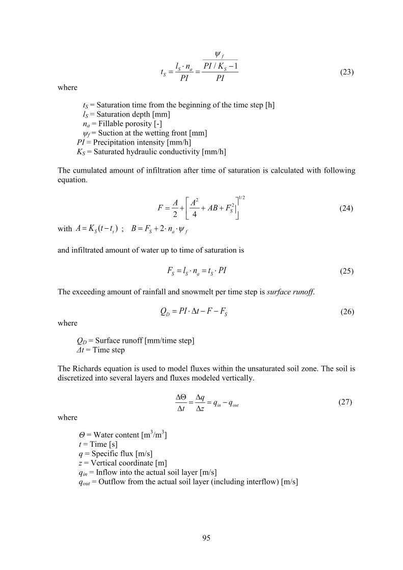
95
/ 1
f
S a SS
l n PI KtPI PI
ψ⋅ −
= = (23)
where
tS = Saturation time from the beginning of the time step [h] lS = Saturation depth [mm] na = Fillable porosity [-] ψf = Suction at the wetting front [mm] PI = Precipitation intensity [mm/h] KS = Saturated hydraulic conductivity [mm/h] The cumulated amount of infiltration after time of saturation is calculated with following equation.
1/22
2
2 4 SA AF AB F
= + + +
(24)
with ( )S sA K t t= − ; 2S a fB F n ψ= + ⋅ ⋅ and infiltrated amount of water up to time of saturation is
S S a SF l n t PI= ⋅ = ⋅ (25) The exceeding amount of rainfall and snowmelt per time step is surface runoff.
D SQ PI t F F= ⋅∆ − − (26) where
QD = Surface runoff [mm/time step] Δt = Time step The Richards equation is used to model fluxes within the unsaturated soil zone. The soil is discretized into several layers and fluxes modeled vertically.
in outq q q
t z∆Θ ∆
= = −∆ ∆
(27)
where
Θ = Water content [m3/m3] t = Time [s] q = Specific flux [m/s] z = Vertical coordinate [m] qin = Inflow into the actual soil layer [m/s] qout = Outflow from the actual soil layer (including interflow) [m/s]

96
Calculations of interflow are performed if suction in a particular layer holds less than 3.45 m. Two values for interflow are calculated from different equations (equations (28) and (29)) and the smaller one gives the result.
( ),max 3.45( )iflzqtψψ =
∆= Θ −Θ ⋅
∆ (28)
where
Θ(ψ) = Water content at actual suction (ψ) [-] Θψ=3.45 = Water content at suction ψ=3.45 m [-] Δz = Layer thickness [-]
Δt = Time step [s] ( ) tanifl s m rq k z d β= Θ ⋅∆ ⋅ ⋅ (29) where
ks = Saturated hydraulic conductivity [m/s] Θs = Water content in the actual layer m [-] dr = Scaling parameter to consider e.g. river density [m-1] β = Local slope angle (if β > 45°, β = 45°) [°] The recession constant krec has to be specified for each soil type to describe the change in recession of the saturated conductivity with depth.
,z
s z s reck k k= ⋅ (30) where
ks,z = Saturated hydraulic conductivity within depth z [m/s] ks = Saturated hydraulic conductivity at the soil surface [m/s] krec = Recession constant [-] z = Depth [m] The baseflow in WaSiM is calculated as exfiltration from groundwater into the river system and is only generated at the grid cells which are marked as river cells. The exfiltration is calculated in two steps, first by using the hydraulic gradient and the colmation at the river bed and then by calculating exfiltration until the suction of 3.45 m is reached. , /exf pot k rbq l H b cs= ⋅∆ ⋅ (31) where
qexf,pot = Maximum possible exfiltration (base flow) [m/s] lk = Leakage factor (colmation resistance) [s-1] ΔH = Positive difference between groundwater table and river bed brb = Width of the river bed [m] cs = Grid cell size [m]
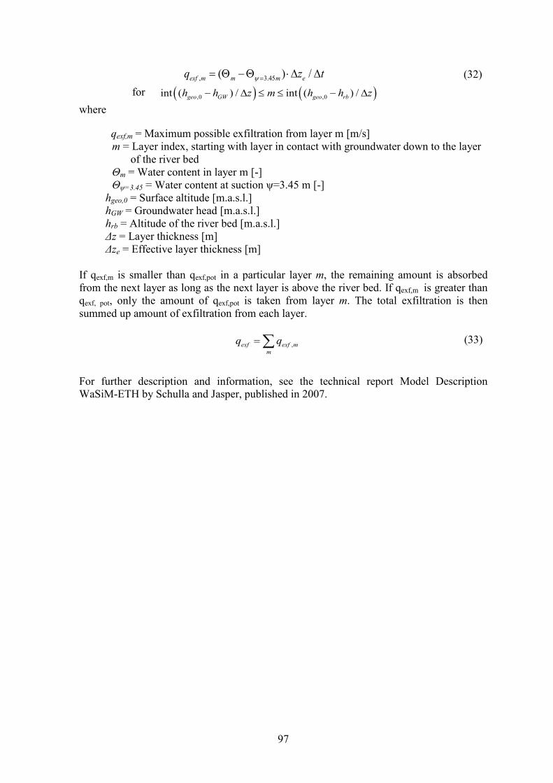
97
, 3.45( ) /exf m m m eq z tψ == Θ −Θ ⋅∆ ∆ (32) for ( ) ( ),0 ,0int ( ) / int ( ) /geo GW geo rbh h z m h h z− ∆ ≤ ≤ − ∆ where
qexf,m = Maximum possible exfiltration from layer m [m/s] m = Layer index, starting with layer in contact with groundwater down to the layer
of the river bed Θm = Water content in layer m [-] Θψ=3.45 = Water content at suction ψ=3.45 m [-]
hgeo,0 = Surface altitude [m.a.s.l.] hGW = Groundwater head [m.a.s.l.] hrb = Altitude of the river bed [m.a.s.l.] Δz = Layer thickness [m] Δze = Effective layer thickness [m]
If qexf,m is smaller than qexf,pot in a particular layer m, the remaining amount is absorbed from the next layer as long as the next layer is above the river bed. If qexf,m is greater than qexf, pot, only the amount of qexf,pot is taken from layer m. The total exfiltration is then summed up amount of exfiltration from each layer. ,exf exf m
mq q=∑ (33)
For further description and information, see the technical report Model Description WaSiM-ETH by Schulla and Jasper, published in 2007.


99
Appendix II -Maps of Dynjandisá River
Following are maps of the Dynjandi catchment, where the hydropower potential is shown in more details. The hydropower results are shown with two maps for each runoff scenario, corresponding to the two domains that are marked with the numbers 1 and 2 on the maps in Chapter 4.
Figure 50: Detailed map of hydropower potential in Dynjandisá River according to mean discharge, map no. 1.
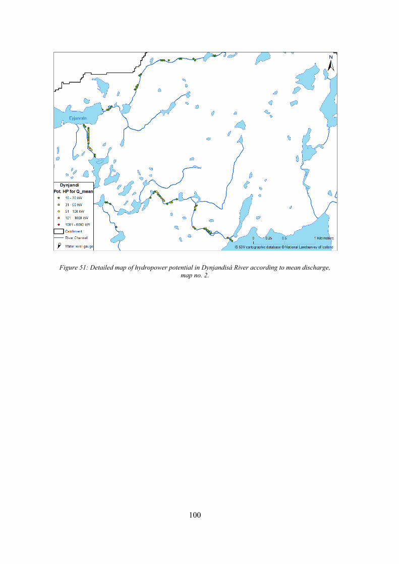
100
Figure 51: Detailed map of hydropower potential in Dynjandisá River according to mean discharge, map no. 2.
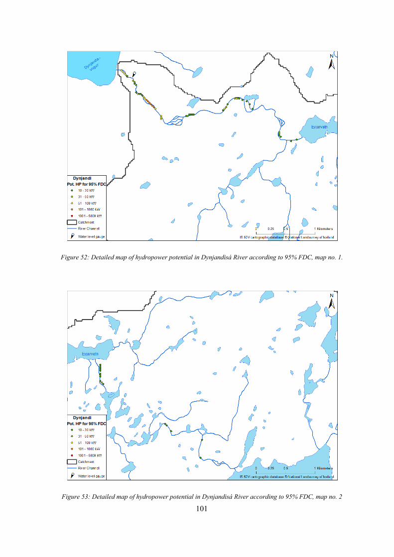
101
Figure 52: Detailed map of hydropower potential in Dynjandisá River according to 95% FDC, map no. 1.
Figure 53: Detailed map of hydropower potential in Dynjandisá River according to 95% FDC, map no. 2

102
Figure 54: Detailed map of hydropower potential in Dynjandisá River according to 85% FDC, map no. 1.
Figure 55: Detailed map of hydropower potential in Dynjandisá River according to 85% FDC, map no. 2.

103
Figure 56: Detailed map of hydropower potential in Dynjandisá River according to 75% FDC, map no. 1.
Figure 57: Detailed map of hydropower potential in Dynjandisá River according to 75% FDC, map no. 2.

104
Figure 58: Detailed map of hydropower potential in Dynjandisá River according to 65% FDC, map no. 1.
Figure 59: Detailed map of hydropower potential in Dynjandisá River according to 65% FDC, map no. 2.
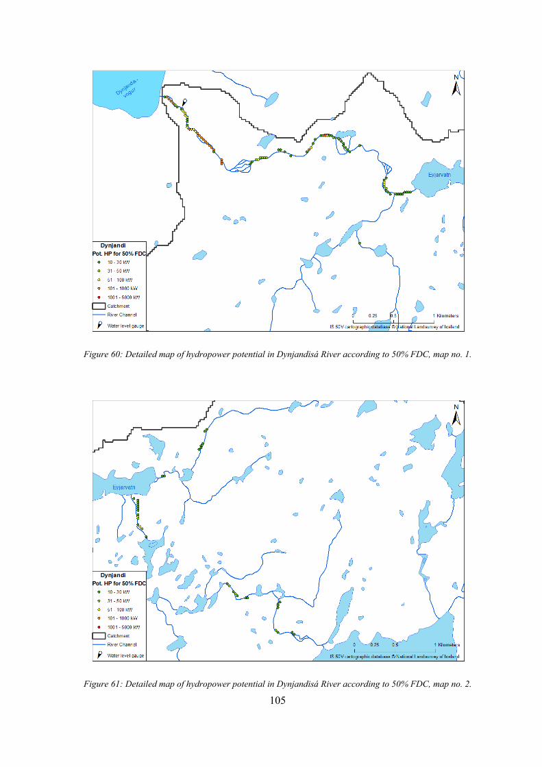
105
Figure 60: Detailed map of hydropower potential in Dynjandisá River according to 50% FDC, map no. 1.
Figure 61: Detailed map of hydropower potential in Dynjandisá River according to 50% FDC, map no. 2.

106
Figure 62: Detailed map of hydropower potential in Dynjandisá River according to 10% FDC, map no. 1.
Figure 63: Detailed map of hydropower potential in Dynjandisá River according to 10% FDC, map no. 2