Development Economics Research Group

Development Economics Research Group Working Paper Series 04-2020

Does Scarcity Reduce Cooperation? Experimental Evidence from Rural Tanzania

Gustav Agneman Paolo Falco Exaud Joel Onesmo Selejio

October 2020 ISSN 2597-1018

https://www.econ.ku.dk/derg/

Does Scarcity Reduce Cooperation?Experimental Evidence from Rural Tanzania∗

Gustav Agneman1, Paolo Falco1, Exaud Joel2, and Onesmo Selejio2

1Department of Economics, University of Copenhagen2Department of Economics, University of Dar Es Salaam

October 21, 2020

Abstract

Cooperation is essential to reap efficiency gains from specialization, not least in poor com-munities where economic transactions often are informal. Yet, cooperation might be moredifficult to sustain under scarcity, since defecting from a cooperative equilibrium can yieldsafe, short-run benefits. In this study, we investigate how scarcity affects cooperation byleveraging exogenous variation in economic conditions induced by the Msimu harvest in ru-ral Tanzania. We document significant changes in food consumption between the pre- andpost-harvest period, and show that lean season scarcity reduces socially efficient but per-sonally risky investments in a framed Investment Game. This can contribute to what iscommonly referred to as a behavioral poverty trap.

Keywords: scarcity, cooperation, field experimentJEL Codes: C71, C93, D91

∗This study was made possible by financial support from the Danish Embassy in Dar es Salaam(Tanzania), as part of the GDRP Phase II Project. We are grateful to the team of researchassistants from the Singida region for their excellent work. We are also thankful to the DevelopmentEconomics Research Group at the University of Copenhagen for their invaluable support, and to theTRIBE group at the University of Copenhagen for great feedback. The research was approved by theTanzania Commission for Science and Technology (COSTECH) and pre-registered in the AmericanEconomic Association registry for randomized controlled trials (ID: AEARCTR-0005794).

1 Introduction

Many economic transactions rest on mutual trust and cooperation, and self-enforced compli-

ance is thus essential for the functioning of markets. Countries, organisations, and communi-

ties with higher levels of trust have recurrently been shown to attain better economic results

(e.g., Algan and Cahuc 2010; Bohnet, Herrmann, and Zeckhauser 2010; Knack and Keefer

1997; La Porta et al. 1997). However, cooperative equilibria are inherently unstable, since

defection can yield safe and short-run private benefits (Dal Bó and Fréchette 2011). This

is particularly a problem in developing countries where contracts are hard to enforce and

informality is widespread. In order to better understand obstacles to economic development,

we therefore ought to map factors that underpin or undermine economic cooperation.

In this paper, we ask whether adverse economic conditions, and in particular the

experience of food scarcity, can lead to a breakdown in cooperation. We hypothesize that

people invest less in cooperative solutions when resources are scarce, since scarcity increases

the relative cost of defection by others. As a consequence, agents may forego investment

opportunities that are both individually profitable and socially efficient.

Our study takes place in the poverty-stricken region Singida, Tanzania, where we

document significant variation in food scarcity between the pre-harvest (early May) and the

post-harvest (mid-July) period. We exploit this exogenous variation in food supply to study

how scarcity impacts farmers’ willingness to engage in cooperative behaviour, by measuring

cooperation both before and after the harvest through a lab-in-the-field experiment. Invest-

ing is socially efficient and potentially profitable from the investor’s perspective, but the

outcome is uncertain as it rests on reciprocation from another agent.

We find that scarcity depresses cooperation. Before the harvest, when farmers face

greater food shortages, they invest significantly less compared to after the harvest. The

reduced form impact is significant both in a between-subject design (different participants

before and after the harvest) and a within-subject design (the same subjects participating

twice). Intuitively, the effects are substantially larger for relatively poorer farmers, who ex-

perience greater scarcity in the pre-harvest period. We further corroborate the interpretation

of the effect as one driven by food scarcity by means of an instrumental variable approach.

1

Our study extends a growing literature on the relationship between poverty and eco-

nomic behavior, which encompasses studies on e.g. self-control (Banerjee and Mullainathan

2010), risk-aversion (Yesuf and Bluffstone 2009 and Blalock, Just, and Simon 2007), and

borrowing choices (Shah, Mullainathan, and Shafir 2012 and Agarwal, Skiba, and Tobac-

man 2009). In particular, we contribute to the emergent literature concerned with the causal

effect of scarcity on economic behaviors (e.g., Miguel 2005; Shah, Mullainathan, and Shafir

2012; Haushofer, Schunk, and Fehr 2013; Prediger, Vollan, and Herrmann 2014; Shah, Shafir,

and Mullainathan 2015; Carvalho, Meier, and Wang 2016; Lichand et al. 2020). Our identi-

fication strategy builds on the seminal study by Mani et al. (2013), who exploit the timing

of sugar cane harvests in India to investigate how scarcity influences cognitive abilities.

A few studies have previously investigated links between seasonal scarcity and ad-

verse behavior in the context of Tanzania (most notably the study by Miguel (2005) on

witch-hunts)). Closely related with the present study, Hadley, Mulder, and Fitzherbert

(2007) find that “instrumental social support” – meaning economic support in case of need

– associates negatively and strongly with incidences of food scarcity in South-western Tan-

zania. They draw the conclusion that social support determines food scarcity. While a lack

of cooperation could aggravate food scarcity, our findings suggest that the impact also runs

in the opposite direction: scarcity depresses cooperation.

We differ from previous studies on scarcity and economic behavior in a number of

important respects. First, by investigating the influence of scarcity on potentially self-serving

cooperation, our conceptualization of cooperation contrasts with studies measuring behavior

in, e.g., one-shot prisoner’s dilemmas (Boonmanunt and Meier 2020) and joy-of-destruction

games (Prediger, Vollan, and Herrmann 2014). Cooperating in a one-shot prisoner’s dilem-

mas can be interpreted as an act of altruism, since defecting is invariably personally prof-

itable. In the real world, decisions on whether to cooperate or not depend crucially on

potential personal gains from successful cooperation. The sequential way in which senders

and receivers interact in the Investment Game allows us to capture cooperation motivated

also by personal interest; cooperation in our study is a risky but potentially profitable op-

tion.1

1. Indeed, altruistic motives are not a dominant predictor of behavior in the Investment Game (Brülhart

2

Second, we distinguish our work from previous research by focusing on food scarcity

as opposed to scarcity of financial resources (Mani et al. 2013; Aksoy and Palma 2019;

Boonmanunt and Meier 2020). In e.g. Mani et al. (2013), the sampled farmers are able to

smooth food consumption and are not eating less prior to the harvest. In our context, a

substantial proportion of the farmers do not accumulate any savings, and are forced to reduce

food consumption in the lean period. While food and financial scarcity are correlated, food

scarcity is a more severe form of deprivation and can be expected to trigger larger behavioral

changes (Schofield 2014). Our results confirm this hypothesis. To the best of our knowledge,

we are the first to document how food scarcity depresses socially efficient investment.

Third, by instrumenting scarcity using the post-harvest shock in food supply as an

instrument, we go further than studies focusing exclusively on the reduced form impact of

the harvest (Mani et al. 2013; Bartos 2016; Aksoy and Palma 2019; Boonmanunt and Meier

2020). Using a two-stage least squares approach, we are able to document that scarcity is

indeed the mediating channel depressing cooperation in the lean period.

The paper is structured as follows. In Section 2, we discuss relevant features of the

Singida region, the empirical context of the present study. Section 3 outlines our experimental

design and in Section 4 we present the main findings. We discuss the implications of the

findings in Section 5.

2 Empirical setting: the region of Singida

The study was conducted in Singida, a poverty-stricken region in central Tanzania with a

diverse population. In our sample, the Nyaturu (36%), Sukuma (25%), and Gogo (23%)

constitute the main ethnic groups, 63% adhere to Christianity, whereas 26% are Muslims.

The region is semi-arid and the economy heavily centered around agricultural production.

Food crops are the dominant products: 9 out of 10 participants in our sample grow maize,

1 in 5 grows sorghum, and 1 in 5 grows millet. Sweet potatoes and sunflower seeds, which

are sometimes used for food consumption and sometimes as cash crops, are cultivated by

15% and 40% of the farmers, respectively. While the timing of the harvest varies somewhat

and Usunier 2012).

3

between crops, the main harvesting period is between May and June.

The harvest constitutes the main source of income and food for the farmers of

Singida; in our sample, 88.1% of the respondents report that (at least) some of their income

comes from farming. Hence, consumption can vary significantly between the lean pre-harvest

period and the abundant post-harvest period (as we later show in Section 4.1). The variation

is accentuated by major obstacles to consumption smoothing, such as credit constraints and

limited access to saving mechanisms. Poor farmers – like the participants in our study

– tend to lack reliable storage opportunities, both in terms of food (Parfitt, Barthel, and

Macnaughton 2010) and in terms of cash (Aryeetey 1997). Saving is risky due to a weak

justice system (Bates 1987). Lastly, present bias may further enhance seasonal fluctuations

in food availability (Laajaj 2017), as a preference for immediate consumption may contribute

to depleting surpluses, especially among people who can barely satisfy their basic needs.

3 Experimental design

Our analysis is centered around an Investment Game (Berg, Dickhaut, and McCabe 1995),

which we conduct before and after the yearly harvest, with participants from two distinct sets

of randomly selected villages in the region of Singida. In this section, we outline the Invest-

ment Game, introduce two experimental manipulations, and discuss our sampling strategy.

3.1 The Investment Game

We conduct an Investment Game à la Berg, Dickhaut, and McCabe (1995). The game has

two players (A and B) who are anonymous to each other (they never meet and their decisions

are only reported to the other player after the game is concluded). Player A begins the game

with a certain endowment and chooses how much to invest in a common project with Player

B. The amount s/he invests is then tripled and Player B gets to split the income from the

investment between the two players. For simplicity, Player A could choose to invest all, half,

or none of the initial endowment.

To facilitate understanding, the game was framed as a situation familiar to farmers:

Player A had to decide how much to invest in seeds that would result in a harvest worth

4

three times the investment. The initial endowment Player A was given amounted to 4,000

Tanzanian Shillings, roughly corresponding to a day’s worth of the minimum wage in the

agricultural sector in Tanzania (De Blasis 2020). S/he was informed that Player B would

decide how the income from the harvest would be split between the two players. The payoffs

were paid in cash at the end of the day, after the game and an accompanying survey were

completed. The rules of the game were explained carefully by means of examples and visual

aids. The full script and the visual aids are shown in Appendix B. In Figure 1 we depict the

sequencing of the game.

Figure 1: Decision tree

Player A {4,000}

(4, 000)

0

Player B

(2, 000 + (2, 000 × 3 − X1))

X1

2, 000

Player B

(4, 000 × 3 − X2)

X2

4, 000

Figure 1 displays the decision tree and thereby the information set of Player A when making the initialinvestment (or not). The amount in curly brackets refer to the initial endowment of Player A. The amountsin parentheses indicate the potential payoffs of Player A. X1 and X2 denote the sum that Player B decides tokeep for herself, respectively in the scenarios when 2,000 and 4,000 was invested by Player A. X1 is boundedbetween 0 and 6,000, whereas X2 is bounded between 0 and 12,000.

Based on these rules, Player A was asked to indicate how much s/he wanted to

invest. Player B, on the other hand, was asked to indicate how much s/he would give back

to Player A for each level of investment Player A could have made (the actual choice made

by Player A was not revealed until after the game and the ensuing interview was concluded).

In order to minimize experimenter demand effects that might be caused by the presence of

interviewers, participants were asked to make their choice in a private space by indicating

their decision on a sheet. They were then asked to fold the answer sheet and hand it back

to the enumerator (who did not look at their answer until later).

5

3.2 Manipulations

The primary focus of this study is how cooperation depends on participants’ current food

situation. We hypothesize that food scarcity hampers respondents’ ability to choose the

socially efficient option of investing, by leading them to prefer a safe option (not investing).

We rely on the seasonal variation in food scarcity induced by the harvest to identify the causal

effect of food scarcity on investment. In addition, we embed two experimental treatments

in the Investment Game: (a) a prime that makes scarcity particularly salient prior to the

game; (b) an ingroup/outgroup manipulation.

3.2.1 Scarcity prime

A growing literature has documented the psychological impacts of poverty on decision-

making (Shah, Shafir, and Mullainathan 2015; Lichand et al. 2020). At least to some extent,

it is the awareness of trade-offs (e.g. between risk and reward) – what Mullainathan and

Shafir (2013) label a scarcity mindset – which influences behavior. In our context, this means

that in addition to scarcity influencing behavior directly, when a current state of scarcity is

made salient it should depress investment further. To trigger this mechanism, we asked re-

spondents a series of questions about their current food consumption (we detail the questions

in Figure A2 in the Appendix). Half of our respondents (primed) are asked those questions

before they play the Investment Game. The other half (control) answers those questions

after they play the game.

3.2.2 Ingroup vs Outgroup

Our second experimental manipulation is employed to test whether scarcity is more dam-

aging for cooperation with people who are more socially distant. This may be the case, for

instance, if social proximity makes reciprocity easier to sustain. We test this proposition by

randomly varying the counterpart that respondents face in the Investment Game (i.e., Player

B) between an ingroup and an outgroup member. Specifically, while half of the participants

are told that Player B is another (anonymous) person from their own village, the rest are

told that Player B is from another part of Tanzania. The ingroup/outgroup manipulation

6

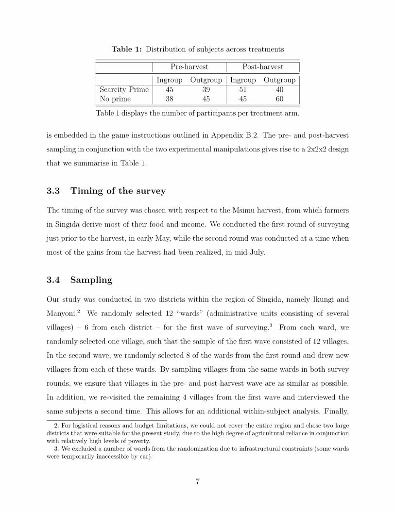
Table 1: Distribution of subjects across treatments

Pre-harvest Post-harvestIngroup Outgroup Ingroup Outgroup

Scarcity Prime 45 39 51 40No prime 38 45 45 60

Table 1 displays the number of participants per treatment arm.

is embedded in the game instructions outlined in Appendix B.2. The pre- and post-harvest

sampling in conjunction with the two experimental manipulations gives rise to a 2x2x2 design

that we summarise in Table 1.

3.3 Timing of the survey

The timing of the survey was chosen with respect to the Msimu harvest, from which farmers

in Singida derive most of their food and income. We conducted the first round of surveying

just prior to the harvest, in early May, while the second round was conducted at a time when

most of the gains from the harvest had been realized, in mid-July.

3.4 Sampling

Our study was conducted in two districts within the region of Singida, namely Ikungi and

Manyoni.2 We randomly selected 12 “wards” (administrative units consisting of several

villages) – 6 from each district – for the first wave of surveying.3 From each ward, we

randomly selected one village, such that the sample of the first wave consisted of 12 villages.

In the second wave, we randomly selected 8 of the wards from the first round and drew new

villages from each of these wards. By sampling villages from the same wards in both survey

rounds, we ensure that villages in the pre- and post-harvest wave are as similar as possible.

In addition, we re-visited the remaining 4 villages from the first wave and interviewed the

same subjects a second time. This allows for an additional within-subject analysis. Finally,

2. For logistical reasons and budget limitations, we could not cover the entire region and chose two largedistricts that were suitable for the present study, due to the high degree of agricultural reliance in conjunctionwith relatively high levels of poverty.

3. We excluded a number of wards from the randomization due to infrastructural constraints (some wardswere temporarily inaccessible by car).

7

to increase statistical power, in the second wave we also included two new villages from

randomly selected wards that were not part of the first round.

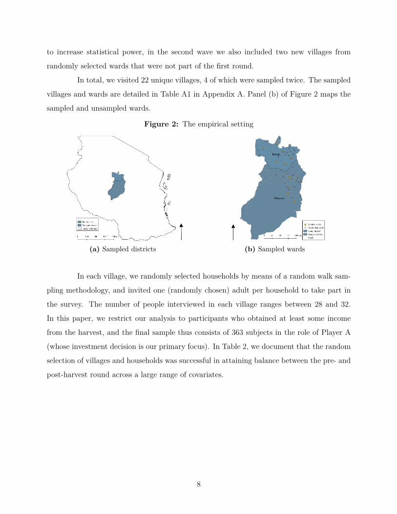
In total, we visited 22 unique villages, 4 of which were sampled twice. The sampled

villages and wards are detailed in Table A1 in Appendix A. Panel (b) of Figure 2 maps the

sampled and unsampled wards.

Figure 2: The empirical setting

(a) Sampled districts (b) Sampled wards

In each village, we randomly selected households by means of a random walk sam-

pling methodology, and invited one (randomly chosen) adult per household to take part in

the survey. The number of people interviewed in each village ranges between 28 and 32.

In this paper, we restrict our analysis to participants who obtained at least some income

from the harvest, and the final sample thus consists of 363 subjects in the role of Player A

(whose investment decision is our primary focus). In Table 2, we document that the random

selection of villages and households was successful in attaining balance between the pre- and

post-harvest round across a large range of covariates.

8

Table 2: Covariates balance between the pre- and the post-harvest sample

Pre-harvest Post-harvestN Mean S.d. N Mean S.d. Difference

Woman 167 0.44 0.50 196 0.46 0.50 0.021Age 167 42.92 14.72 196 41.65 13.76 -1.274Years in village 167 23.13 15.97 196 26.06 18.02 2.924Non-farm earnings 167 0.10 0.30 196 0.13 0.33 0.026Post-primary education 167 0.11 0.31 196 0.14 0.35 0.030Literacy 167 0.84 0.36 196 0.87 0.34 0.023Muslim 167 0.30 0.46 196 0.22 0.42 -0.075Christian 167 0.58 0.49 196 0.66 0.47 0.082Nyaturu 167 0.37 0.48 196 0.36 0.48 -0.008Sukuma 167 0.25 0.44 196 0.25 0.43 -0.001Gogo 167 0.21 0.41 196 0.24 0.43 0.035Head of household 167 0.71 0.45 196 0.64 0.48 -0.075Married 167 0.83 0.37 196 0.82 0.38 -0.011Owns cattle 167 0.53 0.50 196 0.51 0.50 -0.028Owns chickens 167 0.77 0.42 196 0.74 0.44 -0.033Owns goats 167 0.46 0.50 196 0.42 0.50 -0.032Maize cropping 167 0.90 0.30 196 0.86 0.35 -0.047Sunflower seed cropping 167 0.38 0.49 196 0.44 0.50 0.067Sorghum cropping 167 0.20 0.40 196 0.22 0.42 0.021Millet cropping 167 0.18 0.39 196 0.19 0.39 0.009Owns tractor 167 0.01 0.11 196 0.00 0.00 -0.012Owns plough 167 0.47 0.50 196 0.44 0.50 -0.028Using fertilizer 167 0.10 0.30 196 0.12 0.33 0.021Rain irrigation 167 0.99 0.08 196 0.99 0.07 0.001Recent family death 167 0.02 0.13 196 0.02 0.14 0.002Recent property theft 167 0.05 0.23 196 0.07 0.26 0.018Receives financial/food support 167 0.13 0.33 196 0.08 0.27 -0.044Has outstanding loan 167 0.24 0.43 196 0.21 0.41 -0.025

Table 2 shows descriptive statistics on a range of relevant covariates for the pre- and post-harvestsample. The Difference column displays coefficients and corresponding significance levels from simplea regression with post-harvest treatment as the sole regressor and robust standard errors. * p < 0.10,** p < 0.05, *** p < 0.01.

4 Results

In this section, we present the results of our analysis. First, we document large variation

in food scarcity between the pre- and post-harvest period. Second, we present evidence of

a significant change in cooperative behavior between the two periods. Third, we estimate a

causal impact of food scarcity on cooperative behavior by instrumenting the level of scarcity

with an dummy variable indicating whether the Investment Game was played in the lean- or

9

abundant period. Fourth, we show that the results are robust to accounting for a broad set of

potential confounders. Fifth, we document the impact of the two experimental manipulations

embedded in the Investment Game. Finally, we show that cooperation on average paid off.

4.1 The harvest changes scarcity levels

The first step in our analysis is to investigate whether reliance on a yearly harvest leads

to fluctuations in food scarcity among the farmers in our sample. We find a substantial

effect of the harvest on levels of food scarcity. Figure 3 plots histograms of how frequently

people did not have sufficient food in the month prior to the survey. It shows a clear shift in

the distribution with the share of people declaring food shortages falling significantly after

the harvest. While 7 out of 10 households reported some degree of food scarcity before the

harvest, only 3 out of 10 did so after the harvest.

Figure 3: Effect of harvest on scarcity

Figure 3 displays the change in food scarcity from round 1 to round 2. Food scarcity is measured as theresponse to the following question: “Over the past month, how often, if ever, have you or anyone in yourfamily gone without enough food to eat?”.

10

In Table A3 in Appendix C.3, we show that the shift is both statistically significant

and economically meaningful. Scarcity decreased in the post-harvest period by more than

four fifths of a standard deviation. The results are robust to using alternative measures of

food scarcity, namely the number of days with fewer meals than normal over the past month

(see Figure A4 in the Appendix C.1).

4.2 Cooperation is lower before the harvest

Having established a link between the harvest and food scarcity, we can now investigate

how this exogenous source of variation affects investment behavior. We estimate the impact

for four different samples. The Full sample, which includes all farmers in our sample; the

Limited sample, from which we exclude the post-harvest observations on participants that

also took part in the first round4; the Within sample, where we focus on individuals who

participated twice (and can therefore include individual-level fixed effects); and finally the

Village sample, which reports the effect of the harvest on average village-level investment.

In Table 3 we report the results.

Table 3: Effect of the harvest on investment

Dep. Var.: Investment in the Investment Game

Sample: Full Limited Within Village

(1) (2) (3) (4)Post-harvest Treatment 258.8∗∗ 218.6∗ 583.3∗∗ 259.7∗∗

(120.8) (122.2) (265.2) (122.1)Constant 2802.4∗∗∗ 2802.4∗∗∗ 3708.3∗∗∗ 2799.7∗∗∗

(105.1) (105.3) (336.9) (104.0)Observations 363 310 106 26R-squared 0.0112 0.00762 0.550 0.167Dep. Var. Mean 2942.1 2903.2 2849.1 2939.6Individual F.E. NO NO YES NO

Cluster-robust standard errors in parentheses*** p<0.01, ** p<0.05, * p<0.1

Table 3 displays OLS regression estimates of the effect of the harvest on investment inthe Investment Game. Individual F.E. indicates Individual Fixed Effects. All specifica-tions report cluster-robust standard errors at the village-round level.

Regardless of the specification, the results show that cooperation is significantly4. The rationale for this specification is to ensure that learning effects – which may affect behavior of

participants that participated twice – do not influence the findings.

11

lower in the lean period that precedes the harvest. For the full sample presented in column 1,

we document an increase in investment amounting to almost 10% of the baseline investment

level after the harvest. The effect is somewhat smaller and less precisely estimated when we

restrict the analysis to the limited sample, but the effect remains significant at the 10% level.

In column 3, we zoom in on farmers who participated twice and estimate a diff-in-diff model

with individual fixed effects. Once again, the results show a large and positive impact of the

harvest on investment decisions. Lastly, in column 4 we report the impact of the harvest on

average investment at the village level. By studying the effect at this level of aggregation, we

ensure that the results are not sensitive to intra-group correlations in investment behavior

(Angrist and Pischke 2008).5 The positive impact of the harvest is statistically significant

also in this sample.

Finally, we show that the harvest induced a more significant reduction in food

scarcity – and a larger increase in investment – among relatively poorer participants (as

measured by a self-reported evaluation6). In Figure 4, we show that while relatively poor

participants are much more likely to experience scarcity before the harvest, these differences

are largely levelled out by the harvest. Correspondingly, relatively poor farmers increase their

investment levels substantially more compared to the relatively well-off in the post-harvest

period.

5. The main regressions report clustered standard errors at the village-round level for this reason, butgroup averages are somewhat more reliable when the number of clusters is relatively small (Angrist andPischke 2008).

6. The survey item read “How rich or poor is your household in comparison with other households in thevillage? ” (Much poorer; A little poorer; Same; A little richer; Much richer).

12

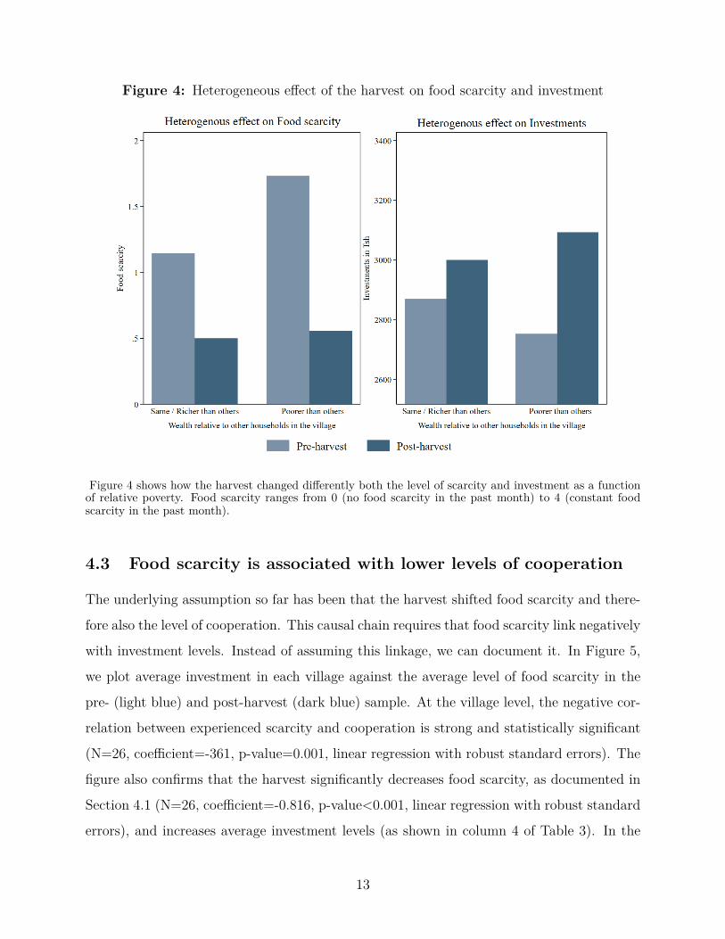
Figure 4: Heterogeneous effect of the harvest on food scarcity and investment

Figure 4 shows how the harvest changed differently both the level of scarcity and investment as a functionof relative poverty. Food scarcity ranges from 0 (no food scarcity in the past month) to 4 (constant foodscarcity in the past month).

4.3 Food scarcity is associated with lower levels of cooperation

The underlying assumption so far has been that the harvest shifted food scarcity and there-

fore also the level of cooperation. This causal chain requires that food scarcity link negatively

with investment levels. Instead of assuming this linkage, we can document it. In Figure 5,

we plot average investment in each village against the average level of food scarcity in the

pre- (light blue) and post-harvest (dark blue) sample. At the village level, the negative cor-

relation between experienced scarcity and cooperation is strong and statistically significant

(N=26, coefficient=-361, p-value=0.001, linear regression with robust standard errors). The

figure also confirms that the harvest significantly decreases food scarcity, as documented in

Section 4.1 (N=26, coefficient=-0.816, p-value<0.001, linear regression with robust standard

errors), and increases average investment levels (as shown in column 4 of Table 3). In the

13

Appendix Section C.2 (Table A2), we also document the negative association between food

scarcity and investment levels at the individual level.

Figure 5: Village-level food scarcity and investment (pre- vs post-harvest sample)

Figure 5 shows the correlation between village level food scarcity and investment. Moreover, the figuredisplays how both the level of scarcity and investment levels changed with the harvest. Food scarcity rangesfrom 0 (no food scarcity in the past month) to 4 (constant food scarcity in the past month).

A mere correlation between food scarcity and investment does not, however, prove

that a lack of food causes lower investment levels. Next, we complete the analysis by inves-

tigating the causal impact of food scarcity on cooperation.

4.4 The causal impact of scarcity on cooperation

We estimate the direct impact of food scarcity on cooperation by means of a standard two-

stage least squares approach, exploiting the harvest as an instrument for food scarcity. For

this strategy to be valid, we need the harvest to have had substantial influence on the levels

of food scarcity. This was demonstrated in Section 4.1. Moreover, we need our pre- and

post-harvest samples to be similar in all respects that matter for cooperation except for

14

food scarcity. Though we cannot be certain that such a restriction is fulfilled, we can use

the information contained in the survey to alleviate concerns that either sampling error or

unaccounted seasonal shocks might threaten the causal interpretation of our results. First,

we showed in Table 2 that the two samples are strongly balanced across a large set of

covariates. In addition, we show in Section 4.5 that while we observe seasonality in other

domains besides food scarcity (e.g., festive events and weather shocks), these factors do not

confound our analysis.

The results from the two-stage least squares regressions are reported in Table 4.

We display estimates for the Full-, Limited-, Within-, and Village-sample. In Panel A, we

show that the harvest is a first-order predictor of food scarcity. The associated F-values

range between 26 and 35, which is evidence of a strong first stage. In Panel B, we outline

the second stage estimates. The results show that scarcity significantly reduces cooperative

behavior. The economic significance is substantial. Since scarcity is measured on a scale from

0 to 4, the linear estimates imply that going from no to constant scarcity would decrease

investment levels from 3209 Tsh to 2105 Tsh, on average. Just like in the reduced form

results in Table 3, the effect is even larger for the difference-in-difference estimation on the

within-subject sample presented in column 3.

15

Table 4: Effect of food scarcity on investment

Panel A: First StageDep. Var.: Food scarcitySample: Full Limited Within Village

(1) (2) (3) (4)Post-harvest Treatment -0.937∗∗∗ -0.907∗∗∗ -1.125∗∗∗ -0.920∗∗∗

(0.160) (0.163) (0.211) (0.157)Constant 1.473∗∗∗ 1.473∗∗∗ 1.063∗∗∗ 1.459∗∗∗

(0.156) (0.156) (0.125) (0.152)Observations 363 310 106 26R-squared 0.169 0.152 0.687 0.621Dep. Var. Mean 0.967 1.055 1.038 0.964F-value 34.86 33.27 28.34 26.85Individual F.E. NO NO YES NO

Panel B: Second StageDep. Var.: Investment in the Investment GameSample: Full Limited Within Village

(1) (2) (3) (4)Food scarcity -276.1∗∗ -241.1∗∗ -518.5∗∗∗ -318.3∗∗∗

(124.0) (114.9) (161.0) (122.8)Constant 3209.2∗∗∗ 3157.5∗∗∗ 4259.3∗∗∗ 3233.2∗∗∗

(114.3) (109.1) (200.2) (111.7)Observations 363 310 106 26Dep. Var. Mean 2942.1 2903.2 2849.1 2939.6Individual F.E. NO NO YES NO


Table 4 displays instrumental variable regression estimates of the effect of food scarcityon investment in the Investment Game. Food scarcity is operated as a continuous vari-able ranging from 0 (no food scarcity in the past month) to 4 (constant food scarcityin the past month) and is instrumented by a dummy for participating in the Invest-ment Game after the harvest. Individual F.E. indicates Individual Fixed Effects. Allspecifications report standard errors clustered at the level of wards.

4.5 Addressing potential confounders

In this subsection we address concerns that time-varying factors other than food scarcity may

have influenced our findings. Based on the existing literature and on the specific context

of our study, we identified four key factors which varied between the pre- and post-harvest

season (see Figure A3 in Appendix C.1) and may have influenced changes in cooperative be-

havior. First, the harvest relaxes financial constraints as well as constraints on the availability

of food (Aksoy and Palma 2019). Many farmers grow cash crops and one may hypothesize

that it is the greater availability of money, rather than increased abundance of food, that

changes people’s decisions in the game. Second, more resources – and a lower workload –

16

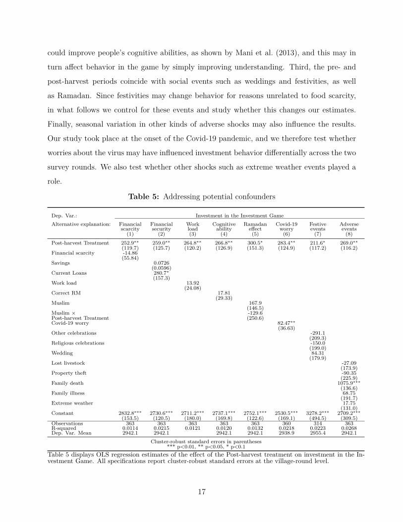
could improve people’s cognitive abilities, as shown by Mani et al. (2013), and this may in

turn affect behavior in the game by simply improving understanding. Third, the pre- and

post-harvest periods coincide with social events such as weddings and festivities, as well

as Ramadan. Since festivities may change behavior for reasons unrelated to food scarcity,

in what follows we control for these events and study whether this changes our estimates.

Finally, seasonal variation in other kinds of adverse shocks may also influence the results.

Our study took place at the onset of the Covid-19 pandemic, and we therefore test whether

worries about the virus may have influenced investment behavior differentially across the two

survey rounds. We also test whether other shocks such as extreme weather events played a

role.

Table 5: Addressing potential confounders

Dep. Var.: Investment in the Investment GameAlternative explanation: Financial Financial Work Cognitive Ramadan Covid-19 Festive Adverse

scarcity security load ability effect worry events events(1) (2) (3) (4) (5) (6) (7) (8)

Post-harvest Treatment 252.9∗∗ 259.0∗∗ 264.8∗∗ 266.8∗∗ 300.5∗ 283.4∗∗ 211.6∗ 269.0∗∗

(119.7) (125.7) (120.2) (126.9) (151.3) (124.9) (117.2) (116.2)Financial scarcity -14.86

(55.84)Savings 0.0726

(0.0596)Current Loans 280.7∗

(157.3)Work load 13.92

(24.08)Correct RM 17.81

(29.33)Muslim 167.9

(146.5)Muslim × -129.6Post-harvest Treatment (250.6)Covid-19 worry 82.47∗∗

(36.63)Other celebrations -291.1

(209.3)Religious celebrations -150.0

(199.0)Wedding 84.31

(179.9)Lost livestock -27.09

(173.9)Property theft -90.35

(225.9)Family death 1075.9∗∗∗

(136.6)Family illness 68.75

(191.7)Extreme weather 17.75

(131.0)Constant 2832.8∗∗∗ 2730.6∗∗∗ 2711.2∗∗∗ 2737.1∗∗∗ 2752.1∗∗∗ 2530.5∗∗∗ 3278.2∗∗∗ 2709.2∗∗∗

(153.5) (120.5) (180.0) (169.8) (122.6) (169.1) (494.5) (309.5)Observations 363 363 363 363 363 360 314 363R-squared 0.0114 0.0215 0.0121 0.0120 0.0132 0.0218 0.0223 0.0268Dep. Var. Mean 2942.1 2942.1 2942.1 2942.1 2938.9 2955.4 2942.1


Table 5 displays OLS regression estimates of the effect of the Post-harvest treatment on investment in the In-vestment Game. All specifications report cluster-robust standard errors at the village-round level.

17

Table 5 shows that the range of hypothesized confounders had little or no impact on

the baseline results. In Appendix C.5, we further corroborate these insights by adding a large

battery of controls (Table A5) and documenting the stability of the effect of the harvest, as

well as of food scarcity, on investment. Moreover, since assignment into the pre- and post-

harvest sample was random by nature, we can study the effect by means of randomization

inference. In Figure A6, we show that the effect of the post-harvest treatment does not

rely on the distributional assumptions invoked in OLS regressions; the effect is estimated

at the same level of statistical significance also when using randomization inference. While

it is impossible to ensure that all the potential confounders are accounted for, the stability

of the post-harvest effect across specifications is reassuring. In the following section, we

further strengthen the interpretation of the scarcity effect by presenting results from our

experimental manipulations.

4.6 Experimental manipulations

Next, we use our experimental manipulations to explore two channels that may play an

important role in aggravating the effect of food scarcity on cooperation. First, we study

whether the effect becomes stronger when scarcity is more salient in respondents’ minds.

Second, we investigate whether scarcity is more harmful for cooperation with people who

are not from the same village and hence typically fall outside the participant’s network of

support.

4.6.1 Perceived scarcity

According to the work by Shah, Mullainathan, and Shafir (2012) and Shah, Shafir, and

Mullainathan (2015), the psychology of scarcity is not only driven by the actual state of

scarcity; rather, a scarcity mind-set can be activated or deactivated dependent on the current

saliency of scarcity. As a consequence, we should expect that shifting attention towards

present scarcity should lower cooperation further. To test this proposition, we experimentally

exposed a subset of participants’ to a scarcity prime which intended to make the state of

scarcity more salient. The prime was a survey section asking respondents questions about

18

consumption, relative wealth, and food shortages they may have recently experienced. Half

of the respondents played the Investment Game after answering these questions, whereas

the other half played before being exposed to them.

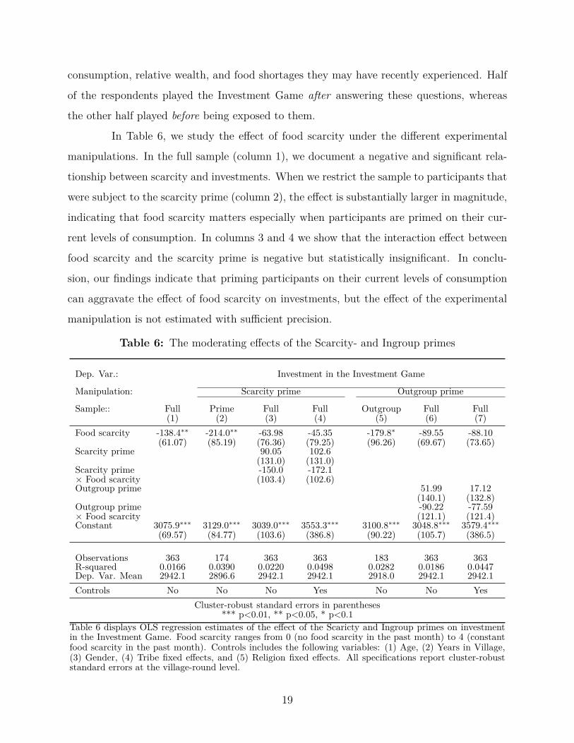
In Table 6, we study the effect of food scarcity under the different experimental

manipulations. In the full sample (column 1), we document a negative and significant rela-

tionship between scarcity and investments. When we restrict the sample to participants that

were subject to the scarcity prime (column 2), the effect is substantially larger in magnitude,

indicating that food scarcity matters especially when participants are primed on their cur-

rent levels of consumption. In columns 3 and 4 we show that the interaction effect between

food scarcity and the scarcity prime is negative but statistically insignificant. In conclu-

sion, our findings indicate that priming participants on their current levels of consumption

can aggravate the effect of food scarcity on investments, but the effect of the experimental

manipulation is not estimated with sufficient precision.

Table 6: The moderating effects of the Scarcity- and Ingroup primes


Manipulation: Scarcity prime Outgroup prime

Sample:: Full Prime Full Full Outgroup Full Full(1) (2) (3) (4) (5) (6) (7)

Food scarcity -138.4∗∗ -214.0∗∗ -63.98 -45.35 -179.8∗ -89.55 -88.10(61.07) (85.19) (76.36) (79.25) (96.26) (69.67) (73.65)

Scarcity prime 90.05 102.6(131.0) (131.0)

Scarcity prime -150.0 -172.1× Food scarcity (103.4) (102.6)Outgroup prime 51.99 17.12

(140.1) (132.8)Outgroup prime -90.22 -77.59× Food scarcity (121.1) (121.4)Constant 3075.9∗∗∗ 3129.0∗∗∗ 3039.0∗∗∗ 3553.3∗∗∗ 3100.8∗∗∗ 3048.8∗∗∗ 3579.4∗∗∗

(69.57) (84.77) (103.6) (386.8) (90.22) (105.7) (386.5)

Observations 363 174 363 363 183 363 363R-squared 0.0166 0.0390 0.0220 0.0498 0.0282 0.0186 0.0447Dep. Var. Mean 2942.1 2896.6 2942.1 2942.1 2918.0 2942.1 2942.1Controls No No No Yes No No Yes


Table 6 displays OLS regression estimates of the effect of the Scaricty and Ingroup primes on investmentin the Investment Game. Food scarcity ranges from 0 (no food scarcity in the past month) to 4 (constantfood scarcity in the past month). Controls includes the following variables: (1) Age, (2) Years in Village,(3) Gender, (4) Tribe fixed effects, and (5) Religion fixed effects. All specifications report cluster-robuststandard errors at the village-round level.

19

4.6.2 Ingroup differentiation

Finally, we study how the effect of scarcity on cooperation varies depending on the identity of

the second player. Previous research has suggested that resource scarcity can enhance group

differentiation and animosity (e.g. Krosch and Amodio 2014), and recent evidence points to

the conclusion that scarcity could exacerbate the negative effects of diversity on cooperation

(Schaub, Gereke, and Baldassarri 2020). In our context, such a mechanism would lead to

food scarcity having a stronger negative effect on cooperation when the second player is from

the outgroup compared to when the second player is part of the ingroup. To investigate this,

we experimentally varied the identity of the second player between someone from the local

village and from another part of Tanzania.7

We find only suggestive evidence that scarcity is more damaging for cooperation

towards outgroup members. In column 5 of Table 6, we show that food scarcity is associated

with lower investment levels when the second player is from the outgroup relative to the base-

line sample (column 1). Put simply, participants that experience scarcity send less money on

average, but the reduction is larger when they are matched with an outgroup member. To

investigate whether the difference is statistically significant, we re-run the analysis over the

entire sample and add an interaction term between the outgroup prime and being exposed

to scarcity (column 6 and 7 of Table 6). While the interaction term is negative (indicating

that people are less cooperative with outgroup members), it is imprecisely estimated and we

cannot conclude that scarcity is more damaging for cooperation towards outgroup members.

In Appendix C.4, we also investigate how trust in the ingroup and outgroup, respec-

tively, influences investment levels in the two experimental treatments. As expected, higher

self-reported trust in the ingroup is associated with higher investment when the subjects are

paired with an ingroup member. Similarly, higher outgroup trust increases investment when

subjects are paired with an outgroup member. We next consider a measure of parochial

trust, which we define as trust in the ingroup minus trust in the outgroup (see Figure A5),

and introduce it in an interaction term with the ingroup treatment. We find that respondents

who declare trusting ingroup members more than outgroup members are more cooperative

7. Since networks of support are often built within a village, this strategy captures a salient ingroup vsoutgroup distinction.

20

with ingroup members in the game, and vice versa.

4.7 Does cooperation pay off?

Throughout the analysis, we have considered higher investment in the game as a positive

result since it is the socially efficient option (the total payoff triples when invested). To

conclude the results section, we investigate whether cooperation is also privately profitable

for investors. Upon deciding how much to invest, Player A faces the risk that Player B

may send back less than the invested amount. The degree to which the investment pays off,

therefore, is conditional on reciprocation.

In Figure 6, we show the distribution of amounts returned by Player Bs when Player

A invests 2,000 and 4,000 Tsh, respectively. The choices of Player Bs were elicited by means

of the strategy method, meaning that participants did not know the actual sum invested but

made conditional choices for the different possible scenarios.

Figure 6: Return on investment

Figure 6 displays the distribution of money sent back by Player B for investments by Player A of 2,000 Tshand 4,000 Tsh, respectively.

Figure 6 confirms that investing did pay off in expectation. For Player A, the

decision to keep the money, e.g. not to invest, would result in a secure payoff of 4,000

21

Tsh. If half instead was invested, the expected payoff would be 4,922 Tsh (the 2,000 the

participant did not invest, plus an average expected return of 2,922 Tsh). If all 4,000 Tsh

were invested, the participant would in expectation receive a payoff of 5,931 Tsh. However,

investing entailed risks, since Player B in some cases decided to send back less than the

initial investment.

5 Discussion

The present study has shown that scarcity of food can depress socially efficient cooperation.

Prior to the harvest – in a state of scarcity – farmers were less likely to make an investment

that could benefit both themselves and another participant in the economic experiment. In

line with Mullainathan and Shafir (2013), we hypothesize that this pattern is due to safer but

low yielding options (not investing) becoming relatively more attractive in times of scarcity.

The effect was lower realized payoffs of both senders and receivers in the lean season relative

to the abundant season. The harvest served as a great (albeit temporary) leveler between

rich and poor, both in terms of food consumption and in terms of investment behavior. In

fact, after the harvest, the relatively poorer farmers were no less likely to invest.

Our findings bear important insights for both researchers and policy makers. Com-

munal cooperation is essential for the efficient functioning of local economies, not least in

rural developing contexts which lack strong formal institutions. Cooperation is conducive to

economic growth, but may also be a by-product of improved economic conditions, in that

economic slack enables people to afford the risks that cooperative behavior entails. This

study supports the latter channel and is the first one, to the best of our knowledge, that

documents a causal link between food scarcity and cooperation. If a shortage of food brakes

down local networks of cooperation, this means that scarcity, even if temporary, can induce

more scarcity in the future. By uncovering the detrimental impacts that deprivation can have

on agents’ willingness to invest, we make an important contribution to our understanding of

behavioral poverty traps.

22

Bibliography

Agarwal, Sumit, Paige Marta Skiba, and Jeremy Tobacman. 2009. “Payday Loans and Credit

Cards: New Liquidity and Credit Scoring Puzzles?” American Economic Review 99 (2):

412–17.

Aksoy, Billur, and Marco A. Palma. 2019. “The Effects of Scarcity on Cheating and In-Group

Favoritism.” Journal of Economic Behavior & Organization 165:100–117.

Algan, Yann, and Pierre Cahuc. 2010. “Inherited Trust and Growth.” American Economic

Review 100 (5): 2060–92.

Angrist, Joshua D, and Jörn-Steffen Pischke. 2008. Mostly harmless econometrics: An em-

piricist’s companion. Princeton university press.

Aryeetey, Ernest. 1997. “Rural Finance in Africa: Institutional Developments and Access for

the Poor.” In Proc. of the Annual World Bank Conference on Development Economics.

Washington DC, 149–154.

Banerjee, Abhijit, and Sendhil Mullainathan. 2010. The Shape of Temptation: Implications

for the Economic Lives of the Poor. Technical report. National Bureau of Economic

Research.

Bartos, Vojtech. 2016. “Seasonal scarcity and sharing norms.” CERGE-EI Working Paper

Series, no. 557.

Bates, Robert H. 1987. Essays on the Political Economy of Rural Africa. Vol. 38. Univ of

California Press.

Berg, Joyce, John Dickhaut, and Kevin McCabe. 1995. “Trust, reciprocity, and social his-

tory.” Games and economic behavior 10 (1): 122–142.

Blalock, Garrick, David R. Just, and Daniel H. Simon. 2007. “Hitting the Jackpot or Hitting

the Skids: Entertainment, Poverty, and the Demand for State Lotteries.” American

Journal of Economics and Sociology 66:545–570.

23

Bohnet, Iris, Benedikt Herrmann, and Richard Zeckhauser. 2010. “Trust and the Reference

Points for Trustworthiness in Gulf and Western Countries.” 125 (2): 811–828.

Boonmanunt, Suparee, and Stephan Meier. 2020. “The Effect of Financial Constraints on

In-Group Bias: Evidence from Rice Farmers in Thailand.”

Brülhart, Marius, and Jean-Claude Usunier. 2012. “Does the trust game measure trust?”

Economics Letters 115 (1): 20–23.

Carvalho, Leandro S., Stephan Meier, and Stephanie W. Wang. 2016. “Poverty and Economic

Decision-Making: Evidence from Changes in Financial Resources at Payday.” American

economic review 106 (2): 260–84.

Dal Bó, Pedro, and Guillaume R Fréchette. 2011. “The Evolution of Cooperation in Infinitely

Repeated Games: Experimental Evidence.” American Economic Review 101:411–429.

De Blasis, Fabio. 2020. “Global horticultural value chains, labour and poverty in Tanzania.”

World Development Perspectives: 100201.

Hadley, Craig, Monique Borgerhoff Mulder, and Emily Fitzherbert. 2007. “Seasonal food

insecurity and perceived social support in rural Tanzania.” Public health nutrition 10

(6): 544–551.

Haushofer, Johannes, Daniel Schunk, and Ernst Fehr. 2013. “Negative Income Shocks In-

crease Discount Rates.”

Knack, Stephen, and Philip Keefer. 1997. “Does Social Capital Have an Economic Payoff?

A Cross-Country Investigation.” The Quarterly Journal of Economics 112 (4): 1251–88.

Krosch, Amy R, and David M Amodio. 2014. “Economic scarcity alters the perception of

race.” Proceedings of the National Academy of Sciences 111 (25): 9079–9084.

La Porta, Rafael, Florencio Lopez de Silane, Andrei Shleifer, and Robert W. Vishny. 1997.

“Trust in Large Organizations.” American Economic Review 87 (2): 333–38.

Laajaj, Rachid. 2017. “Endogenous Time Horizon and Behavioral Poverty Trap: Theory and

Evidence from Mozambique.” Journal of Development Economics 127:187–208.

24

Lichand, Guilherme, Eric Bettinger, Nina Cunha, and Ricardo Madeira. 2020. “The Psycho-

logical Effects of Poverty on Investments in Children’s Human Capital.” University of

Zurich, Department of Economics, Working Paper, no. 349.

Mani, Anandi, Sendhil Mullainathan, Eldar Shafir, and Jiaying Zhao. 2013. “Poverty Impedes

Cognitive Function.” science 341 (6149): 976–980.

Miguel, Edward. 2005. “Poverty and witch killing.” The Review of Economic Studies 72 (4):

1153–1172.

Mullainathan, Sendhil, and Eldar Shafir. 2013. Scarcity: Why having too little means so

much. Macmillan.

Parfitt, Julian, Mark Barthel, and Sarah Macnaughton. 2010. “Food Waste within Food

Supply Chains: Quantification and Potential for Change to 2050.” Philosophical Trans-

actions of the Royal Society B: Biological Sciences 365:3065–3081.

Prediger, Sebastian, Björn Vollan, and Benedikt Herrmann. 2014. “Resource Scarcity and

Antisocial Behavior.” Journal of Public Economics 119:1–9.

Schaub, Max, Johanna Gereke, and Delia Baldassarri. 2020. “Does poverty undermine co-

operation in multiethnic settings? Evidence from a cooperative investment experiment.”

Journal of Experimental Political Science 7 (1): 27–40.

Schofield, Heather. 2014. “The Economic Costs of Low Caloric Intake: Evidence from India.”

Unpublished Manuscript.

Shah, Anuj K., Sendhil Mullainathan, and Eldar Shafir. 2012. “Some Consequences of Having

Too Little.” Science 338 (6107): 682–685.

Shah, Anuj K, Eldar Shafir, and Sendhil Mullainathan. 2015. “Scarcity frames value.” Psy-

chological Science 26 (4): 402–412.

Yesuf, Mahmud, and Randall A. Bluffstone. 2009. “Poverty, Risk Aversion, and Path De-

pendence in Low-Income Countries: Experimental Evidence from Ethiopia.” American

Journal of Agricultural Economics 91 (4): 1022–1037.

25

Appendix

A Sampling strategy

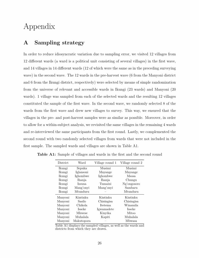
In order to reduce idiosyncratic variation due to sampling error, we visited 12 villages from

12 different wards (a ward is a political unit consisting of several villages) in the first wave,

and 14 villages in 14 different wards (12 of which were the same as in the preceding surveying

wave) in the second wave. The 12 wards in the pre-harvest wave (6 from the Manyoni district

and 6 from the Ikungi district, respectively) were selected by means of simple randomization

from the universe of relevant and accessible wards in Ikungi (23 wards) and Manyoni (20

wards). 1 village was sampled from each of the selected wards and the resulting 12 villages

constituted the sample of the first wave. In the second wave, we randomly selected 8 of the

wards from the first wave and drew new villages to survey. This way, we ensured that the

villages in the pre- and post-harvest samples were as similar as possible. Moreover, in order

to allow for a within-subject analysis, we revisited the same villages in the remaining 4 wards

and re-interviewed the same participants from the first round. Lastly, we complemented the

second round with two randomly selected villages from wards that were not included in the

first sample. The sampled wards and villages are shown in Table A1.

Table A1: Sample of villages and wards in the first and the second round

District Ward Village round 1 Village round 2Ikungi Sepuka Musimi MusimiIkungi Iglansoni Mnyange MnyangeIkungi Ighombwe Ighombwe MsosaIkungi Ihanja Ihanja ChunguIkungi Issuna Tumaini Ng’ongosoroIkungi Mang’onyi Mang’onyi SambaruIkungi Mtunduru – Mtunduru

Manyoni Kintinku Kintinku KintinkuManyoni Sasilo Chisingisa ChisingisaManyoni Chikola Itetema WinamilaManyoni Isseke Igwamadete IssekeManyoni Mkwese Kinyika MitooManyoni Muhalala Kapiti MuhalalaManyoni Makutopora – Mbwasa

Table A1 displays the sampled villages, as well as the wards anddistricts from which they are drawn.

26

B Experimental procedure

B.1 Location of the experiment and introduction

Enumerators visited participants in their homes, and found suitable locations for the inter-

views in the vicinity (a quiet place where the respondent could answer the questions without

being disturbed or influenced by other family members). The interviews were conducted on

tablets using KoBo, a survey software. Participants were informed that the survey was part

of an international research project, but not about the research focus. Moreover, they were

told that the survey included three games which would determine the payoffs they received.

In total, participants could earn a minimum of 1,000 Tsh (≈ 0.44 USD) and a maximum of

31,000 Tsh (≈ 13.5 USD). The analysis in this game is focused entirely on the Investment

Game.

B.2 Game instructions

The Investment Game was explained to respondents using the following script. The game

was played at the beginning of a questionnaire (after some basic questions on demographic

characteristics), except for the group that received our random prime. In that case, the

game instructions followed a module with questions aimed at capturing scarcity of food and

income.

27

Player A instructions: In this game, you are paired with another respondent from YOUR VILLAGE / ANOTHER

PART OF TANZANIA. You will not know who this player is, and he/she will not know who you are, except that you are

from the SAME VILLAGE / ANOTHER PART OF TANZANIA. We will simply call him or her Player B. You begin the

game with 4000 Tsh, which are yours. You own a farm together with player B, who begins the game with 0 Tsh.

You have to decide how much money to spend on seeds. The seeds you will buy will be planted and produce a harvest.

The harvest will be sold by Player B, who will decide how to divide the money between the two of you. You have the

following three options:

(1) You buy 4 000 Tsh worth of seeds. This investment yields 12 000 Tsh when the harvest is sold. Player B then decides

how these 12 000 are divided between the two of you. Player B can take as much from this sum as he/she wants, and

what is left will be yours.

(2) You keep 2 000 Tsh and buy 2 000 Tsh worth of seeds. This investment yields 6 000 Tsh when the harvest is sold.

Player B then decides how these 6 000 are divided between the two of you. Player B can take as much from this as he/she

wants, and what is left will be yours. You will at a minimum receive the 2 000 you kept.

(3) You keep all 4 000 Tsh and do not buy any seeds. With no investment, Player B doesn’t receive any money. You will

receive the 4 000 that you kept.

Let’s try to think of some examples:

• If you decide to buy 4,000 worth of seeds, how much does the investment yield?

• If you decide to buy 4,000 worth of seeds and Player B keeps 6 000 Tsh, how much do you get?

• If you decide to buy 4,000 worth of seeds and Player B keeps all the money obtained from selling the harvest, how

much do you get?

• If you decide to buy 2,000 worth of seeds, how much does the investment yield?

• If you decide to buy 2,000 worth of seeds and Player B keeps 2 000 Tsh, how much do you get?

• If you decide to buy 2,000 worth of seeds and Player B keeps all the money obtained from selling the harvest, how

much do you get?

• If you keep 4 000 Tsh and do not buy any seeds, how much do you get?

• If you keep 4 000 Tsh and do not buy any seeds, how much does Player B get?

Now - please make your decision. Would you like to invest 4 000 (Option 1), invest 2 000 and keep 2000 (Option 2), or

keep your 4 000 Tsh and not invest (Option 3)?

28

Player B instructions: In this game, you are paired with another respondent from YOUR VILLAGE / ANOTHER

PART OF TANZANIA. You will not know who this player is, and he/she will not know who you are, except that you are

from the SAME VILLAGE / ANOTHER PART OF TANZANIA. We will simply call him or her Player A. You begin the

game with 0 Tsh. You own a farm together with player A, who begins the game with 4 000 Tsh. Player A had to make a

decision on how much money to spend on seeds by picking one of the following options:

(1) Buy 4 000 Tsh worth of seeds. If Player A chose this option, the investment would yield 12 000 Tsh when the harvest

was sold. You decide how these 12 000 are divided between the two of you. Player A knew that you can decide to take

as much from this sum as you want, and what is left will belong to him/her.

(2) Keep 2 000 Tsh and buy 2 000 Tsh worth of seeds. If Player A chose this option, the investment would yield 6 000 Tsh

when the harvest was sold. You decide how these 6 000 are divided between the two of you. Player A knew that you can

decide to take as much from this sum as you want, and what is left will belong to him/her (on top of the 2 000 he/she

decided to keep).

(3) Keep all 4,000 Tsh for himself/herself, and not buy any seeds. If Player A chose this option, he/she knew that would

receive 4 000, and that you would not receive any money.

Let’s try to think of some examples:

• If Player A decided to buy 4 000 Tsh worth of seeds, how much did the investment yield?

• If Player A decided to buy 4 000 Tsh worth of seeds, and the harvest yielded 12 000, how much does Player A get

if you keep 4 000 Tsh?



• If Player A decided to buy 2 000 Tsh worth of seeds, how much did the investment yield?





• If Player A decided not to buy any seeds and keep all the 4,000 for himself/herself, how much do you get?

How would you divide the money from selling the harvest between the two of you, if Player A chose to buy 4 000 Tsh

worth of seeds, which yielded 12 000?

How would you divide the money from selling the harvest between the two of you, if Player A chose to buy 2 000 Tsh

worth of seeds, which yielded 6 000?

29

B.3 Visual aids

The game was explained by means of the visual aid shown in Figure A1. A copy of the

visual aid was handed to the respondent and it also served the purpose of an answer sheet.

Respondents were instructed to go to a private space and to make their decision by circling

their preferred option. When this was done, they were told to fold the paper before returning

it. The enumerator would then save the sheet, but not look at it in the presence of the

participant.

Figure A1: Visual Assistance Investment Game(a) Game Sheet Player A (b) Game Sheet Player B

The survey also contained a Dictator Game and a Dice Game (to measure honesty). This

paper focuses only on the Investment Game.

30

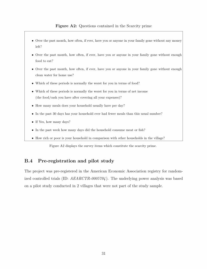
Figure A2: Questions contained in the Scarcity prime

• Over the past month, how often, if ever, have you or anyone in your family gone without any money

left?

• Over the past month, how often, if ever, have you or anyone in your family gone without enough

food to eat?

• Over the past month, how often, if ever, have you or anyone in your family gone without enough

clean water for home use?

• Which of these periods is normally the worst for you in terms of food?

• Which of these periods is normally the worst for you in terms of net income

(the food/cash you have after covering all your expenses)?

• How many meals does your household usually have per day?

• In the past 30 days has your household ever had fewer meals than this usual number?

• If Yes, how many days?

• In the past week how many days did the household consume meat or fish?

• How rich or poor is your household in comparison with other households in the village?

Figure A2 displays the survey items which constitute the scarcity prime.

B.4 Pre-registration and pilot study

The project was pre-registered in the American Economic Association registry for random-

ized controlled trials (ID: AEARCTR-0005794 ). The underlying power analysis was based

on a pilot study conducted in 2 villages that were not part of the study sample.

31

C Results

C.1 Seasonal variation

Figure A3: Seasonal variation

Figure A3 shows a number of potentially confounding factors that vary across the pre- and post-harvestsamples. The confidence intervals are computed based on standard errors clustered at the village-round level.

Figure A4: Farmers have fewer meals than normally before the harvest

Figure A4 shows the average number of days over the previous month when the respondent’s householdhad fewer meals than normal, before and after the harvest. The exact question was: “In the past 30 dayshas your household ever had fewer meals than this usual number? If Yes, how many days?”. The confidenceintervals are computed based on standard errors clustered at the village-round level.

32

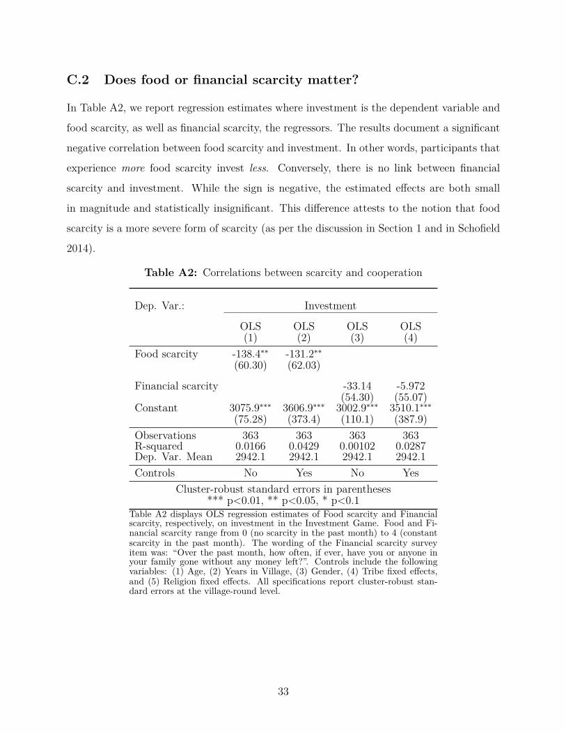
C.2 Does food or financial scarcity matter?

In Table A2, we report regression estimates where investment is the dependent variable and

food scarcity, as well as financial scarcity, the regressors. The results document a significant

negative correlation between food scarcity and investment. In other words, participants that

experience more food scarcity invest less. Conversely, there is no link between financial

scarcity and investment. While the sign is negative, the estimated effects are both small

in magnitude and statistically insignificant. This difference attests to the notion that food

scarcity is a more severe form of scarcity (as per the discussion in Section 1 and in Schofield

2014).

Table A2: Correlations between scarcity and cooperation

Dep. Var.: Investment

OLS OLS OLS OLS(1) (2) (3) (4)

Food scarcity -138.4∗∗ -131.2∗∗

(60.30) (62.03)

Financial scarcity -33.14 -5.972(54.30) (55.07)

Constant 3075.9∗∗∗ 3606.9∗∗∗ 3002.9∗∗∗ 3510.1∗∗∗

(75.28) (373.4) (110.1) (387.9)Observations 363 363 363 363R-squared 0.0166 0.0429 0.00102 0.0287Dep. Var. Mean 2942.1 2942.1 2942.1 2942.1Controls No Yes No Yes


Table A2 displays OLS regression estimates of Food scarcity and Financialscarcity, respectively, on investment in the Investment Game. Food and Fi-nancial scarcity range from 0 (no scarcity in the past month) to 4 (constantscarcity in the past month). The wording of the Financial scarcity surveyitem was: “Over the past month, how often, if ever, have you or anyone inyour family gone without any money left?”. Controls include the followingvariables: (1) Age, (2) Years in Village, (3) Gender, (4) Tribe fixed effects,and (5) Religion fixed effects. All specifications report cluster-robust stan-dard errors at the village-round level.

33

C.3 First stage results

Table A3: Effect of the Harvest on Scarcity

Dep. Var.: Food scarcity Financial scarcity

Ologit OLS OLS Ologit OLS OLS(1) (2) (3) (4) (5) (6)

Post-harvest Treatment -1.631∗∗∗ -0.920∗∗∗ -0.932∗∗∗ -0.606∗∗∗ -0.393∗∗∗ -0.394∗∗∗

(0.209) (0.111) (0.110) (0.189) (0.121) (0.118)Constant 1.456∗∗∗ 1.260∗∗∗ 2.041∗∗∗ 1.502∗∗∗

(0.0915) (0.333) (0.0849) (0.350)Observations 365 365 365 365 365 365R-squared – 0.164 0.217 – 0.0281 0.103Dep. Var. Mean 0.962 0.962 0.962 1.830 1.830 1.830Controls No No Yes No No Yes


Table A3 displays Ologit and OLS regression estimates of the effect of the harvest on a measure of food andfinancial scarcity. Food and Financial scarcity range from 0 (no scarcity in the past month) to 4 (constantscarcity in the past month). The wording of the Financial scarcity survey item was: “Over the past month,how often, if ever, have you or anyone in your family gone without any money left?”. Controls include the fol-lowing variables: (1) Age, (2) Years in Village, (3) Gender, (4) Tribe fixed effects, and (5) Religion fixed effects.All specifications report cluster-robust standard errors at the village-round level.

C.4 Additional results

Figure A5: Parochial trust

Figure A5 shows the distribution of parochial trust. Parochial trust is defined as trust in people from thevillage (a scale from 1 to 5) minus trust in people from other parts of Tanzania (also a scale from 1 to 5).In other words, positive parochial trust means that participants trust the ingroup more than the outgroup,and a negative number indicates the reverse.

34

Table A4: The association between trust and investment

Dep. Var.: Investment in the Investment GameSample: Ingroup Outgroup Full Full

prime prime(1) (2) (3) (4)

Ingroup trust 174.5∗∗∗

(39.45)Outgroup trust 137.7∗∗

(64.62)Ingroup prime -75.50 -48.42

(139.5) (131.2)Parochial trust -147.7∗∗ -137.7∗∗

(59.14) (63.54)Ingroup prime 246.0∗∗∗ 245.0∗∗∗

× Parochial trust (71.50) (75.84)Constant 2375.2∗∗∗ 2535.7∗∗∗ 2979.4∗∗∗ 3533.4∗∗∗

(135.5) (231.2) (100.8) (375.3)Observations 180 183 363 363R-squared 0.0390 0.0191 0.0221 0.0499Dep. Var. Mean 2966.7 2918.0 2942.1 2942.1Controls No No No Yes


Table A4 displays OLS regression estimates of the association between trustand investment. Ingroup trust is defined as trust in people from the village (ascale from 1 to 5), whereas outgroup trust as trust in people from other partsof Tanzania (also a scale from 1 to 5). Controls include the following variables:(1) Age, (2) Years in Village, (3) Gender, (4) Tribe fixed effects, and (5) Re-ligion fixed effects. All specifications report cluster-robust standard errors atthe village-round level.

35

C.5 Robustness checks

Table A5: Effect of scarcity on cooperation: additional controls table


OLS OLS OLS OLS OLS OLS(1) (2) (3) (4) (5) (6)

Post-harvest 234.6∗∗ 244.4∗∗ 240.5∗∗

Treatment (102.3) (90.36) (99.31)Food scarcity -121.3∗ -118.6∗ -133.0∗∗

(64.56) (61.75) (57.90)Constant 3112.3∗∗∗ 3634.5∗∗∗ 4932.9∗∗∗ 3355.0∗∗∗ 3865.2∗∗∗ 5237.2∗∗∗

(115.4) (332.2) (789.5) (88.99) (324.2) (796.2)Observations 363 363 363 363 363 363R-squared 0.0317 0.0637 0.117 0.0351 0.0658 0.121Dep. Var. Mean 2942.1 2942.1 2942.1 2942.1 2942.1 2942.1Ward F.E. Yes Yes Yes Yes Yes YesReligion F.E. No Yes Yes No Yes YesEthnic group F.E. No Yes Yes No Yes YesAge, Woman, Years in village No Yes Yes No Yes YesEducation F.E. No No Yes No No YesEmployment F.E. No No Yes No No YesHH head, HH adults, HH children No No Yes No No Yes


Columns 1-3 of Table A5 display OLS regression estimates of the effect of the harvest on investment whensubsequently adding a large battery of control variables. Similarly, columns 4-6 show the robustness of therelationship between food scarcity and investment levels. Food scarcity ranges from 0 (no scarcity in the pastmonth) to 4 (constant scarcity in the past month). All specifications report cluster-robust standard errors atthe village-round level.

Figure A6: Randomization inference

Figure A6 displays a kernel density from Randomization Inference estimations. The kernel is a distributionof post-harvest-betas obtained from 10,000 permutations of fictional treatment status. The vertical lineshows the estimated effect of the actual treatment assignment, and the corresponding p-value indicates theprobability that such an extreme value would be estimated by chance.

36

Development Economics Research Group

Documents

Transcript of Development Economics Research Group