Development and Implementation of Nagata Patches ...
94
DEPARTAMENTO DE ENGENHARIA MECÂNICA Development and Implementation of Nagata Patches Interpolation Algorithms Dissertação apresentada para a obtenção do grau de Mestre em Engenharia Mecânica na Especialidade de Sistemas de Produção Autor Diogo Mariano Simões Neto Orientadores Marta Cristina Cardoso de Oliveira Luís Filipe Martins Menezes Júri Presidente Professora Doutora Maria Augusta Neto Professora Auxiliar da Universidade de Coimbra Vogais Professor Doutor Luís Filipe Martins Menezes Professor Associado da Universidade de Coimbra Professor Doutor José Luís de Carvalho Martins Alves Professor Auxiliar da Universidade do Minho Professora Doutora Marta Cristina Cardoso de Oliveira Professora Auxiliar da Universidade de Coimbra Coimbra, Julho, 2010
Transcript of Development and Implementation of Nagata Patches ...

DEPARTAMENTO DE
ENGENHARIA MECÂNICA
DDeevveellooppmmeenntt aanndd IImmpplleemmeennttaattiioonn ooff NNaaggaattaa
PPaattcchheess IInntteerrppoollaattiioonn AAllggoorriitthhmmss Dissertação apresentada para a obtenção do grau de Mestre em Engenharia
Mecânica na Especialidade de Sistemas de Produção
Autor
Diogo Mariano Simões Neto
Orientadores
Marta Cristina Cardoso de Oliveira
Luís Filipe Martins Menezes
Júri
Presidente Professora Doutora Maria Augusta Neto
Professora Auxiliar da Universidade de Coimbra
Vogais
Professor Doutor Luís Filipe Martins Menezes
Professor Associado da Universidade de Coimbra
Professor Doutor José Luís de Carvalho Martins Alves
Professor Auxiliar da Universidade do Minho
Professora Doutora Marta Cristina Cardoso de Oliveira
Professora Auxiliar da Universidade de Coimbra
Coimbra, Julho, 2010


Development and Implementation of
Nagata Patches Interpolation Algorithms Acknowledgements
Diogo Mariano Simões Neto i
Acknowledgements
My work on this thesis has benefitted from the support and guidance of several
people in the Experimental and Computer Aided Technology Group whom I wish to
acknowledge. First and foremost, I would like to express my deepest gratitude to my
excellent advisor Professor Marta Cristina Cardoso de Oliveira, for her guidance, support
and endless patience during the course of my M.Sc. degree at the Department of
Mechanical Engineering, University of Coimbra.
I am also grateful to my co-supervisor, Professor Luís Filipe Martins Menezes, for
his insightful comments on my thesis and research, and also for the opportunity that was
given to me to develop my research work at the Center of Mechanical Engineering of the
University of Coimbra (CEMUC). His drive for scientific rigor and excellence in all
aspects of research has been a great source of inspiration for me.
I also wish to thank my former and current colleagues for creating such an easy-
going atmosphere over the years, for a great many coffee breaks and laughs in our
everyday strive to become “better human beings”, and for keeping up that special work
atmosphere. Thank you all for being the persons you are!
Finally, I would like to thank my family and friends for their encouragement and
understanding through all the years.
“Genius is one percent inspiration and ninety nine percent perspiration.”
Thomas A. Edison, Harper's Monthly, 1932.

Development and Implementation of
Resumo Nagata Patches Interpolation Algorithms
ii Diogo Mariano Simões Neto
Resumo
O principal objectivo deste trabalho é o desenvolvimento e implementação de
algoritmos de interpolação com superfícies Nagata para aplicar na descrição de
ferramentas de simulação numérica do processo de estampagem.
A descrição da superfície tem uma importância fundamental na modelação de
problemas de contacto. No entanto, a maioria dos investigadores continua a recorrer a
modelos poliédricos no MEF, que contribuem para uma simplificação excessiva do
modelo, desprezando a curvatura, o que pode introduzir erros significativos de análise.
Recentemente, Nagata (2005) propôs um algoritmo simples para proceder à interpolação
de superfícies e recuperar a sua geometria inicial. A ideia central desta descrição por
superfícies paramétricas consiste na interpolação quadrática de segmentos curvos, com
base nas posições e nos vectores normais nos pontos da fronteira.
Neste trabalho, aplicam-se os algoritmos de interpolação com superfícies Nagata a
modelos poliédricos. Numa primeira etapa, os algoritmos são aplicados à descrição de
superfícies simples (cilindro, esfera e toróide), para os quais é possível determinar a
normal em cada nó com base na função analítica. Procede-se à comparação entre as
superfícies Nagata triangulares e quadrangulares, em termos de eficiência e robustez dos
algoritmos de interpolação local. Na fase seguinte, aplicam-se os algoritmos de
interpolação com superfícies Nagata utilizando diferentes algoritmos de cálculo do vector
normal, em cada ponto, de modo a analisar a influência da precisão deste parâmetro na
qualidade da interpolação Nagata. São propostos diferentes métodos de cálculo do vector
normal, em cada ponto, com base apenas na interpolação disponível no modelo poliédrico,
e a sua eficiência é analisada recorrendo às mesmas geometrias simples. Por último, é
proposto um algoritmo de interpolação com superfícies Nagata que utiliza a informação
disponível no CAD para estimar o vector normal em cada ponto. Este algoritmo permite
aproximar os modelos CAD e CAE, uma vez que possibilita recuperar a geometria original
na interpolação de superfícies discretizadas.
São apresentadas as ferramentas desenvolvidas para a visualização e análise,
qualitativa e quantitativa, das superfícies Nagata. Finalmente, são propostas algumas

Development and Implementation of
Nagata Patches Interpolation Algorithms Resumo
Diogo Mariano Simões Neto iii
orientações para a geração dos modelos poliédricos, de modo a garantir a precisão da
interpolação com superfícies Nagata.
Palavras-chave: Superfícies Nagata, Interpolação local, Aproximação
de vectores normais, Modelação de ferramentas,
Visualização.

Development and Implementation of
Abstratct Nagata Patches Interpolation Algorithms
iv Diogo Mariano Simões Neto
Abstract
The main objective of this work is the development and implementation of Nagata
patches interpolation algorithms to be used in the description of tools for the numerical
simulation of sheet metal forming.
Surface description accuracy is of paramount importance when modelling contact
problems. However, most FEM researchers still resort to polyhedral models to describe
contact surfaces, which can oversimplify the original system by neglecting the curvature. A
simple algorithm for interpolating discretized surfaces and recover the original geometry
was recently proposed by Nagata (2005). The main idea behind this parametric surface
description is the quadratic interpolation of a curved segment, from the position and
normal vectors at the end points.
In this work, Nagata patches algorithms are first applied to interpolate polyhedral
meshes of simple geometries (cylinder, sphere and torus) where the normal vectors in each
node are provided by analytical functions. The use of triangular or quadrilateral Nagata
patches is compared, both in terms of efficiency and robustness of the local interpolation
algorithm. Afterwards, the interpolation algorithms are applied using different normal
vectors approximations, to analyse the influence of the normal vector accuracy in the
Nagata interpolation accuracy. Several methods for estimating the normal vector from
polyhedral models are analyzed and their efficiency is studied, using the same simple
geometries. Finally, the Nagata patch algorithms are applied to interpolate polyhedral
meshes, using the interpolation available in the original CAD geometry to estimate the
normal vectors. This algorithm allows bridging the gap between CAD and CAE models,
since it allows the interpolation of discretized surfaces recovering the original CAD
geometry.
Tools for Nagata patch visualization and qualitative and quantitative analysis were
also developed and presented. Finally, some guidelines for polyhedral mesh generation, in
order to guarantee accurate Nagata patch interpolation, are proposed.
Keywords: Nagata patches, Local interpolation, Normal vector
approximation, Tools modeling, Visualization.

Development and Implementation of
Nagata Patches Interpolation Algorithms Contents
Diogo Mariano Simões Neto v
Contents
List of Figures ...................................................................................................................... vii
List of Tables ......................................................................................................................... x
Symbology and Acronyms ................................................................................................... xi
Symbology ........................................................................................................................ xi
Acronyms ........................................................................................................................ xii
1. Introduction .................................................................................................................. 1
1.1. Background ............................................................................................................. 1
1.2. Present Status of Tool Descriptions ........................................................................ 3
1.3. Aims of the Work ................................................................................................... 5
1.4. Thesis Structure ...................................................................................................... 6
2. Nagata Patch Formulation ............................................................................................ 7
2.1. Interpolation of an Edge ......................................................................................... 8
2.2. Interpolation of a Triangular Patch ......................................................................... 9
2.3. Interpolation of a Quadrilateral Patch ................................................................... 11
3. Nagata Patches Applied to Simple Geometries ......................................................... 13
3.1. Geometries in 2D Space ....................................................................................... 13
3.1.1. Arc of a Circle Described by Nagata ............................................................. 14
3.2. Geometries in 3D Space ....................................................................................... 18
3.2.1. Interpolation Applied to a Plane .................................................................... 19
3.2.2. Interpolation Applied to a Cylinder ............................................................... 21
3.2.3. Interpolation Applied to a Sphere .................................................................. 26
3.2.4. Interpolation Applied to a Torus ................................................................... 32
4. Vertex Normal Vector Estimative .............................................................................. 38
4.1. Vertex Normal Algorithms ................................................................................... 38
4.1.1. Mean Weighted Equally ................................................................................ 39
4.1.2. Mean Weighted by Angle .............................................................................. 39
4.1.3. Mean Weighted by Sine and Edge Length Reciprocals ................................ 39
4.1.4. Mean Weighted by Areas of Adjacent Triangles .......................................... 40
4.1.5. Mean Weighted by Edge Length Reciprocals ............................................... 40
4.1.6. Mean Weighted by Square Root of Edge Length Reciprocals ...................... 40
4.2. Algorithms Applied to Simple Geometries .......................................................... 41
4.2.1. Algorithms Applied to the Cylinder .............................................................. 41
4.2.2. Algorithms Applied to the Sphere ................................................................. 43
4.2.3. Algorithms Applied to the Torus ................................................................... 45
4.3. Influence of the Normal Vector Estimative in the Nagata Patch Description ...... 47
4.3.1. Cylinder Approximated with Normal Vectors Estimative ............................ 47
4.3.2. Sphere Approximated with Normal Vectors Estimative ............................... 48
4.3.3. Torus Approximated with Normal Vectors Estimative ................................. 50
5. Normal Vector Evaluated from CAD Geometry ....................................................... 53
5.1. Vertex Normal Algorithm Evaluated using NURBS ............................................ 53
5.1.1. Definition and Properties of NURBS Surfaces ............................................. 53
5.1.2. Algorithm Description ................................................................................... 55
Development and Implementation of
Contents Nagata Patches Interpolation Algorithms
vi Diogo Mariano Simões Neto
5.2. Algorithm Applied to the U-shape Tool ............................................................... 56
6. Guidelines to Mesh Generation and Patch Visualization .......................................... 59
6.1. Nagata Patch Visualization ................................................................................... 59
6.1.1. Visualization with Excel® ............................................................................ 59
6.1.2. Visualization with GID® Software ............................................................... 60
6.2. Guidelines to Mesh Generation ............................................................................ 61
6.2.1. Structured and Unstructured Meshes ............................................................ 61
6.2.2. Geometry with Inflection Points ................................................................... 64
6.3. Output Files Description ....................................................................................... 67
7. Conclusions ................................................................................................................ 68
8. References .................................................................................................................. 72
9. Appendix A – IGES Format File ............................................................................... 75
10. Appendix B – Projection of a Point on a NURBS Surface ........................................ 76
11. Appendix C – Derivatives of a NURBS Surface ....................................................... 78
12. Appendix D – Output Files ........................................................................................ 80

Development and Implementation of
Nagata Patches Interpolation Algorithms List of Figures
Diogo Mariano Simões Neto vii
List of Figures
Figure 1. Schematic representation of the deep drawing process.......................................... 1
Figure 2. Surface descriptions used in FEA: (a) parametric description; (b) finite element
mesh description; (c) point data description. ......................................................................... 3
Figure 3. Edge interpolation. ................................................................................................. 9
Figure 4. Triangular patch interpolation: (a) sketch; (b) parameters domain. ..................... 10
Figure 5. Quadrilateral patch interpolation: (a) sketch; (b) parameters domain. ................ 11
Figure 6. Interpolation of a unitary arc of a circle: (a) discretized by 1 element; (b)
discretized by 2 elements. .................................................................................................... 15
Figure 7. Errors in polyhedral models of a unitary arc of a circle: (a) radial error; (b)
normal vector error. ............................................................................................................. 16
Figure 8. Radial error: (a) distribution at the arc of a circle for 1 and 2 elements; (b)
maximum as a function of the edge length. ......................................................................... 16
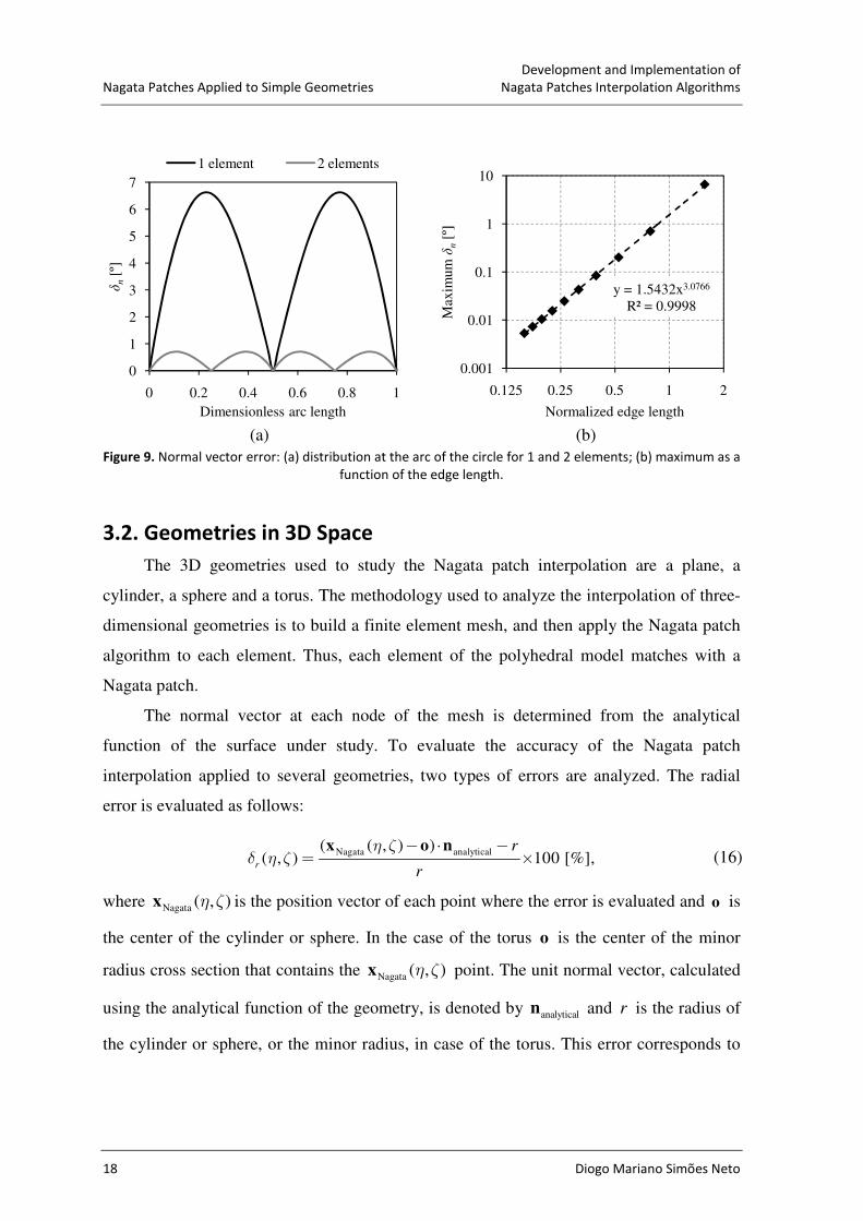
Figure 9. Normal vector error: (a) distribution at the arc of the circle for 1 and 2 elements;
(b) maximum as a function of the edge length. ................................................................... 18
Figure 10. Plane described by: (a) triangular elements; (b) quadrilateral elements. ........... 20
Figure 11. Geometrical error on the plane. .......................................................................... 20
Figure 12. Cylinder described by: (a) triangular elements; (b) quadrilateral elements. ...... 21
Figure 13. Radial and normal vector errors on the triangular patches for the cylindrical
surface. ................................................................................................................................. 22
Figure 14. Errors in the cylindrical surface described by triangular patches: (a) localization
of the cross section A-A; (b) radial and normal vector errors in the cross section A-A. .... 23
Figure 15. Errors in the cylindrical surface described by 2 elements in axial direction: (a)
localization of the cross section A-A; (b) radial and normal vector errors in the cross
section A-A. ......................................................................................................................... 24
Figure 16. Radial and normal vector error on the quadrilateral patches for the cylindrical
surface. ................................................................................................................................. 25
Figure 17. Comparison between triangular and quadrilateral patches for the mesh 1 of the
cylinder: (a) radial error; (b) normal vector error. ............................................................... 26
Figure 18. Sphere described by: (a) triangular elements; (b) quadrilateral elements. ......... 27
Figure 19. Nagata patch error distributions for the sphere described by triangular elements.
............................................................................................................................................. 28
Figure 20. Error distribution in the sphere described by triangular elements: (a) radial error;
(b) normal vector error. ....................................................................................................... 28
Figure 21. Nagata patch error distributions on the triangular patch for the sphere
discretized by quadrilateral elements. ................................................................................. 29
Figure 22. Radial and normal vector errors on the quadrilateral patches when the sphere is
described by quadrilateral elements. ................................................................................... 30
Figure 23. Radial error distribution for the spherical surface discretized with quadrilateral
elements: (a) mesh 1; (b) mesh 2. ........................................................................................ 31
Figure 24. Normal vector error distribution for the spherical surface discretized with
quadrilateral elements: (a) mesh 1; (b) mesh 2.................................................................... 32
Figure 25. Torus described by: (a) triangular elements; (b) quadrilateral elements. ........... 33
Development and Implementation of
List of Figures Nagata Patches Interpolation Algorithms
viii Diogo Mariano Simões Neto
Figure 26. Radial and normal vector errors on the triangular patches used to describe the
torus. .................................................................................................................................... 34
Figure 27. Radial and normal vector errors on the quadrilateral patches used to describe the
torus. .................................................................................................................................... 35
Figure 28. Radial error distribution on the Nagata patches used to describe the torus
surface. ................................................................................................................................ 36
Figure 29. Normal vector error distribution on the Nagata patches used to describe the
torus surface. ....................................................................................................................... 37
Figure 30. Notation used to calculate the normal vector at vertex j . ................................. 38
Figure 31. Normal vector approximation error attained for each algorithm applied to mesh
2 of the cylinder. .................................................................................................................. 42
Figure 32. Maximum normal vector approximation error for the various algorithms applied
to the cylinder described with triangular elements. ............................................................. 42
Figure 33. Normal vector approximation error attained for each algorithm applied to
triangular mesh 2 of the sphere. .......................................................................................... 44
Figure 34. Normal vector approximation error attained for each algorithm applied to
quadrilateral mesh 2 of the sphere. ...................................................................................... 44
Figure 35. Maximum normal vector approximation error for the various algorithms applied
to the sphere. ....................................................................................................................... 45
Figure 36. Normal vector approximation error attained for each algorithm applied to
triangular mesh of the torus (mesh 1). ................................................................................. 45
Figure 37. Normal vector approximation error attained for each algorithm applied to
quadrilateral mesh of the torus (mesh 1). ............................................................................ 46
Figure 38. Maximum normal vector approximation error for the various algorithms applied
to the torus: (a) triangular mesh; (b) quadrilateral mesh. .................................................... 46
Figure 39. Radial and normal vector errors on the triangular patches used to describe the
cylinder (mesh 2) when the MWE algorithm is used to estimate the normal vectors. ........ 48
Figure 40. Radial and normal vector errors on the triangular patches used to describe the
sphere (mesh 2) when the MWA algorithm is used to estimate the normal vectors. .......... 48
Figure 41. Nagata patch radial error in the sphere description (mesh 2) using different
algorithms to estimate the normal vector: (a) maximum; (b) minimum. ............................ 49
Figure 42. Maximum normal vector error at the Nagata patches of the sphere using
different algorithms to estimate the normal vector in each node (mesh 2). ........................ 50
Figure 43. Radial and normal vector errors on the triangular patches used to describe the
torus (mesh 1) when the MWSELR algorithm is used to estimate the normal vectors. ..... 50
Figure 44. Nagata patch radial error in the torus description (mesh 1) using different
algorithms to estimate the normal vector: (a) maximum; (b) minimum. ............................ 51
Figure 45. Maximum normal vector error at the Nagata patches of the torus using different
algorithms to estimate the normal vector in each node (mesh 1). ....................................... 52
Figure 46. Example of a NURBS surface and its bidirectional control net. ....................... 55
Figure 47. Algorithm used to evaluate the normal vector from CAD geometry. ............... 55
Figure 48. Discretized die model in mm: (a) without planes; (b) with planes. ................... 56
Figure 49. Radial error along the cross section A-A, using several methods to calculate the
normal vectors. .................................................................................................................... 57
Figure 50. Visualization of Nagata patches using MS Excel®. .......................................... 60
Figure 51. Visualization of Nagata patches using the GID® software. .............................. 61
Figure 52. Unstructured mesh of a sphere composed by: (a) triangular elements; (b)
quadrilateral elements. ........................................................................................................ 62

Development and Implementation of
Nagata Patches Interpolation Algorithms List of Figures
Diogo Mariano Simões Neto ix
Figure 53. Radial and normal vector errors on the triangular patches used to describe the
sphere. .................................................................................................................................. 62
Figure 54. Radial and normal vector errors on the quadrilateral patches used to describe the
sphere. .................................................................................................................................. 63
Figure 55. Elements with different sizes to describe a 2D geometry with curvature
variation. .............................................................................................................................. 63
Figure 56. Localization for the node near of inflection point. ............................................. 64
Figure 57. Geometry used to analyze the presence of inflection points: (a) NURBS surface;
(b) quadrilateral mesh. ......................................................................................................... 65
Figure 58. Representation of the interpolation using: (a) GID® software; (b) the Excel®
for the xOy plane. ................................................................................................................ 66
Figure 59. Strategy to identify inflection points on a NURBS curve. ................................. 66
Figure 60. Projection of a point on a NURBS surface. ....................................................... 76
Figure 61. First order derivatives in a point of a NURBS surface. ..................................... 78

Development and Implementation of
List of Tables Nagata Patches Interpolation Algorithms
x Diogo Mariano Simões Neto
List of Tables
Table 1. Main characteristics of the meshes used to describe the cylinder. ........................ 21
Table 2. Main characteristics of the meshes used to describe the sphere. .......................... 27
Table 3. Main characteristics of the meshes used to describe the torus. ............................. 33

Development and Implementation of
Nagata Patches Interpolation Algorithms Symbology and Acronyms
Diogo Mariano Simões Neto xi
SYMBOLOGY AND ACRONYMS
Symbology
Cn – n -order continuity
Gn – n -order geometric continuity
( )ξx – Nagata curve
ξ – Nagata curve parametric coordinate
ξx – Nagata curve derivative
c – Vector adding curvature to the Nagata curve
( , )η ζx – Nagata patch
and η ζ – Nagata patch parametric coordinates
and η ζx x – Nagata patch first order partial derivatives
rδ – Radial error
nδ – Normal vector error
analyticaln – Unit normal vector evaluated using the analytical function
Nagatan – Unit normal vector of the Nagata curve or patch
in – Unit normal vector of the thi plane (element)
ie – Edge vector
iα – Angle between the two edge vectors ie and
1i+e
� – Two parallel vectors
⊗ – Cross product of two vectors
θ – Normal vector approximation error
( )uC – NURBS curve
and u v – Parametric coordinates of a NURBS curve or surface
and p q – B-Spline basic function degree in the u and v directions
, ( )i pR u – Rational basic functions of degree p
Development and Implementation of
Symbology and Acronyms Nagata Patches Interpolation Algorithms
xii Diogo Mariano Simões Neto
, ( )i pN u – Normalized B-Spline basic functions of degree p
iP – NURBS curve control points
iw – Weight of each control point iP
and U V – Knot vectors
( , )u vS – NURBS surface
, ( , )i jR u v – NURBS surface rational basic functions
,i jP – NURBS surface control points
,i jw – Weight of each control point ,i jP
and u vS S – NURBS surface first order partial derivatives
, and uu vv uvS S S – NURBS surface second order partial derivatives
Acronyms
2D – Two Dimensional
3D – Three Dimensional
CAD – Computer Aided Design
CAE – Computer Aided Engineering
FEA – Finite Element Analysis
FEM – Finite Element Method
IGES – Initial Graphics Exchange Specification
MWA – Mean Weighted by Angle
MWAAT – Mean Weighted by Areas of Adjacent Triangles
MWE – Mean Weighted Equal
MWELR – Mean Weighted by Edge Length Reciprocals
MWRELR – Mean Weighted by Square Root of Edge Length Reciprocals
MWSELR – Mean Weighted by Sine and Edge Length Reciprocals
NURBS – Non Uniform Rational B-Spline
Development and Implementation of
Nagata Patches Interpolation Algorithms Introduction
Diogo Mariano Simões Neto 1
1. INTRODUCTION
1.1. Background
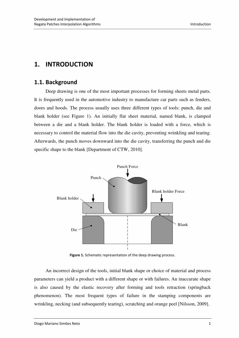
Deep drawing is one of the most important processes for forming sheets metal parts.
It is frequently used in the automotive industry to manufacture car parts such as fenders,
doors and hoods. The process usually uses three different types of tools: punch, die and
blank holder (see Figure 1). An initially flat sheet material, named blank, is clamped
between a die and a blank holder. The blank holder is loaded with a force, which is
necessary to control the material flow into the die cavity, preventing wrinkling and tearing.
Afterwards, the punch moves downward into the die cavity, transferring the punch and die
specific shape to the blank [Department of CTW, 2010].
Figure 1. Schematic representation of the deep drawing process.
An incorrect design of the tools, initial blank shape or choice of material and process
parameters can yield a product with a different shape or with failures. An inaccurate shape
is also caused by the elastic recovery after forming and tools retraction (springback
phenomenon). The most frequent types of failure in the stamping components are
wrinkling, necking (and subsequently tearing), scratching and orange peel [Nilsson, 2009].
Die
Blank holder
Blank
Punch
Punch Force
Blank holder Force
Development and Implementation of
Introduction Nagata Patches Interpolation Algorithms
2 Diogo Mariano Simões Neto
Without the proper knowledge about the influence of process and material variables
on the deep drawing process, it is hardly possible to design the tools adequately and make
a correct choice concerning the blank material and lubrication conditions, to manufacture a
product with the desired shape and performance. As a result, after the first tool design and
choice of blank material and lubricant, an extensive and time consuming trial and error
process is started, to determine the proper tool design and all other variables, which can
lead to the desired product. However, this trial and error process can yield an unnecessary
and expensive number of experimental tests, or may even require the redesign of the
expensive tools. To reduce this waste of time and cost, computer simulation process
modeling can be used to replace the experimental trial and error process by a virtual trial
and error one [Nilsson, 2009].
Nowadays, the Finite Element Method (FEM) is used worldwide to simulate deep
drawing processes. Nevertheless, it is important to mention that, in order to correctly
simulate the physical deep drawing process, it is necessary to accurately describe the tools
geometry, the material behavior, the contact with friction behavior, as well as the other
process variables.
The numerical simulation of sheet metal forming processes is still a complex task.
One of the main reasons for this complexity is the fact that this type of processes is highly
non-linear due to three main reasons. The first is the non-linear kinematic behavior
resulting from large displacements, large rotations and large strains. The second is the non-
linear constitutive behavior of the material, due to the inelastic characteristic of
deformations. The third is the non-linear characteristic of boundary conditions, due to the
interaction between bodies (sheet and tools) along a contact surface that is constantly
changing during the process. All these difficulties make the numerical simulation of sheet
metal forming processes a complex task [Santos, 1993]. The finite element method allows
reproducing reasonably well sheet metal forming process. However, for detailed complex
models the computational cost is high [Skordos et al., 2005].
Presently, the numerical simulation accuracy and consistency does not always satisfy
the industrial necessities, which are always more demanding in terms of time and
complexity of the products. Therefore, an extensive research in this field is still necessary
to decrease the existing gap between the real deep drawing process and the numerical
predictions. The geometric description of the tools surface is one of the fundamental

Development and Implementation of
Nagata Patches Interpolation Algorithms Introduction
Diogo Mariano Simões Neto 3
aspects for treating the non-linear contact with friction problem, always present in the
numerical simulation of deep drawing processes.
1.2. Present Status of Tool Descriptions
Different strategies for tools description in Finite Element Analysis (FEA) were
surveyed and compared by Santos and Makinouchi (1995):
� Analytical functions, in which the surface is modeled using an assembly of
simple geometries (planes, cylinders, spheres and tori);
� Parametric patches, in which the surface is described by an assembly of patches,
e.g., by Bézier, NURBS or B-Spline parametric functions (Figure 2 (a));
� Mesh, in which the surface is descritized by finite element meshes (Figure 2 (b));
� Point data, in which the surface is defined by a collection of points regularly
distributed in xy plane (Figure 2 (c)).
(a) (b) (c)
Figure 2. Surface descriptions used in FEA: (a) parametric description; (b) finite element mesh description;
(c) point data description.
Each of the previously mentioned methods has its own advantages (☺) and
disadvantages (�) [Santos and Makinouchi, 1995].
� Analytical functions:
☺ Fast contact search algorithms;
� Does not allow describing tools with complex geometry.
x
yz
x
yz
x
yz
z
x
y
x
z
x
y
x
z
x
y
x

Development and Implementation of
Introduction Nagata Patches Interpolation Algorithms
4 Diogo Mariano Simões Neto
� Parametric patches:
☺ Direct and efficient data transfer between Computer Aided Design (CAD) and
FEA;
☺ Efficient contact search algorithms;
� Geometry not free of gaps or C0 discontinuity;
� Existence of several kinds of surface entities like Bézier, NURBS and B-Spline. It
is important to define a standard in order to assure easy tool data compatibility.
� Mesh:
☺ Capable of describing any complex tool without limitations;
� Although ensuring the C0 continuity of the surface, C
1 continuity is impossible to
reach.
� Point data:
☺ High speed of contact analysis;
☺ Easy data generation for complex geometries;
� Impossibility or difficulty in describing vertical surfaces, because points are
generated in the xy plane in regular distribution;
� Complex formulation to obtain tool-curvature terms.
Tool surfaces described with C0 and C
1 continuities are desirable and essential
conditions for guaranteeing the efficiency of the contact algorithms, numerical stability and
convergence speed of the simulations [Alves, 2003]. However, most FEM researchers still
resort to polyhedral models, particularly with low order finite elements, to describe contact
surfaces. Sometimes this can lead to large errors in curvature definition, which in turn
affect the accuracy of the numerical simulations results. Thus, over the last years much
research has focused on smooth local interpolations. In 1992, S. Mann et al. concluded that
none of the triangular interpolators’ methods available at that time were satisfactory. After
that, Loop (1994) proposed a sextic triangular Bézier patch to define a G1 spline surface.
The scheme has free parameters which can be used to enforce the surface to interpolate
given mesh vertices, but this often gives rise to undulations of the result. The degenerate
polynomial patches by Neamtu and Pfluger (1994) attain completely local smooth
interpolation from a triangular mesh with normal vectors given at its vertices. The
algorithm involves free parameters also. The triangular G1 interpolation suggested by

Development and Implementation of
Nagata Patches Interpolation Algorithms Introduction
Diogo Mariano Simões Neto 5
Hahmann and Bonneau (2000) is valid for meshes of arbitrary topological type. Their
algorithm was modified to allow completely free tangent directions of the mesh boundary
curves (Hahmann and Bonneau, 2003). The use of polyhedral models also contributes with
difficulties for developing efficient algorithms to solve contact problems, since they need
to accommodate sudden changes in the surface normal field.
The use of parametric surfaces seems the best solution to avoid problems in
curvature definition. However, their use requires solving the information problems related
with the communications between CAD and FEM programs [Alves, 2003]. A simple
algorithm for interpolating discretized surfaces and recover the original geometry was
recently proposed by Nagata (2005, 2010). This new type of surface, subsequently named
Nagata patch, was originally developed to bridge the technical gap between CAD and
numerical simulation.
1.3. Aims of the Work
The main objective of this thesis is the development and implementation of Nagata
patches interpolation algorithms for the representation of surface geometry, either
described by CAD or polyhedral models. In order to evaluate the Nagata interpolation it is
also necessary to develop algorithms for error evaluation.
Two strategies for surface interpolation will be explored:
(1) Based only on the information available from a general polyhedral mesh
description. This implies the exploitation of different approaches to determine
the average normal of each vertex;
(2) Adding to the general polyhedral mesh description the normal of each vertex,
evaluated from CAD geometry.
The comparison of both strategies will help to identify the best approach to determine the
average normal of each vertex, when using only information regarding the nodes position.
Also, strategies for evaluated the error associated to the Nagata patch interpolated
geometry must be developed, considering the two more important errors: the shape and
normal vector errors. Moreover, it is important to develop a procedure for Nagata patch
visualization, allowing a qualitative error analysis.
Development and Implementation of
Introduction Nagata Patches Interpolation Algorithms
6 Diogo Mariano Simões Neto
1.4. Thesis Structure
In order help the reader through the consultation of this dissertation, this section
presents the structure of the work, as well as a brief summary of the topics covered in each
chapter.
Chapter 1 – Discusses the present status of the numerical simulation of sheet metal
forming processes, with particular emphasis for the tool descriptions. Defines and
justifies the objectives for the present work.
Chapter 2 – Describes the distinctive features of the Nagata patch formulation as well as
the formulations for both triangular and quadrilateral patches.
Chapter 3 – The Nagata patch algorithms are applied to interpolate polyhedral meshes,
used to discretize models defined by analytical functions. Thus, this section validates
and evaluates the efficiency of the implemented algorithms.
Chapter 4 – Presents various algorithms to approximate the normal vector at each node of
the polyhedral mesh. These algorithms are applied to geometries with known normal
vectors, in order to evaluate its efficiency. Afterwards, the Nagata interpolation is
applied to the same geometries, to evaluate the influence of the accuracy of the
normal vector in the overall Nagata patch interpolation performance.
Chapter 5 – Describes a method to calculate the normal vector from CAD geometry. The
CAD format file used in this work is the IGES Standard format, which allows
retrieving the interpolation concerning NURBS surfaces. The algorithm is applied to
deep drawing tool geometry and its efficiency is analyzed.
Chapter 6 – Presents the proposed strategies to perform the Nagata patch visualization and
qualitative and quantitative analysis of the interpolation. Some details concerning the
polyhedral models generation are discussed. Base on this analysis, the chapter
presents some guidelines for polyhedral mesh generation in order to improve the
Nagata patch interpolation.
Chapter 7 – Presents the summary of the main conclusions withdrawn from the work
presented in the previous chapters.

Development and Implementation of
Nagata Patches Interpolation Algorithms Nagata Patch Formulation
Diogo Mariano Simões Neto 7
2. NAGATA PATCH FORMULATION
Nagata patch is a simple algorithm for surface interpolation recently proposed by
Nagata (2005), using as central idea the quadratic interpolation of a curved segment, from
the position and normal vectors at the end points. The methodology has the following
distinctive features:
(1) Uses the minimum degree (two) of interpolation, necessary for the surface
curvature representation.
(2) The approach is simple, computationally inexpensive, and hence amenable to
various physical evaluations. The low degree is desirable especially for implicit
contact algorithms, since closed-form solutions may be obtained.
(3) Since the formulation accounts for discontinuity (multiplicity) of normals, sharp
edges and singular points, as well as non-manifolds, can be treated quite easily.
(4) The C0 continuity is always attained, and converges to the original surface
rapidly with the increase in the number of patches. Hence error in the normals
can be sufficiently small using rather few patches.
(5) The algorithm is completely local, requiring only the position vectors and
normals given at the vertices of each patch, hence it is suitable for parallel
processing.
The algorithm may be applied to either smooth or surfaces with discontinuous
normals. However, this work will focus on its application to smooth surfaces, since
surfaces with discontinuous normals are uncommon in tool design.
The Nagata patch interpolation method has already been applied successfully to
engineering problems, including: (i) high-precision machining data generation for an
aspherical lens; and (ii) simulation of elastoplastic 3D continuum dynamics. For both types
of problems the usage of traditional sophisticated surface descriptions is prohibited, due to
severe tolerance as well as geometrical and physical complexity of the systems [Nagata,
2005].

Development and Implementation of
Nagata Patch Formulation Nagata Patches Interpolation Algorithms
8 Diogo Mariano Simões Neto
The following sections describe the Nagata patch interpolation method for both
triangular and quadrilateral patches.
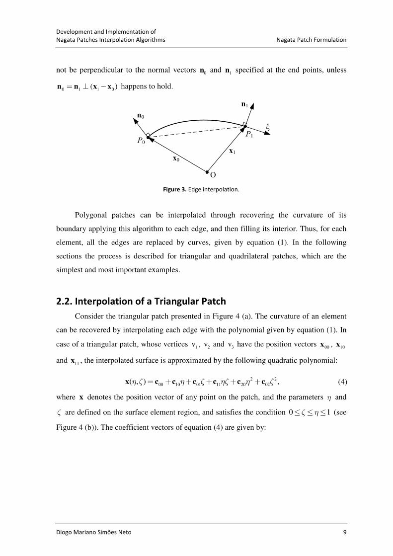
2.1. Interpolation of an Edge
Consider a curve on a surface, as shown in Figure 3, defined by its end points 0P and
1P , with position vectors 0x ,
1x and unit normal vectors 0n ,
1n , respectively, given as input
data. The interpolation of the 0P ,
1P edge is replaced by a curve in the form:
2
0 1 0( ) ( ) ,ξ ξ ξ= + − − +x x x x c c (1)
where ξ is a parameter satisfying the condition 0 1ξ≤ ≤ . The derivative of the Nagata
curve given in equation (1) is:
1 0
d( ) (2 1) ,
d
xx x x cξ ξ
ξ≡ = − + − (2)
which should be orthogonal to the normal vectors 0n and
1n at the end points 0 ( 0)P ξ =
and 1 ( 1)P ξ= , i.e. satisfies the boundary conditions. The derivative of the curve gives the
tangential direction, necessary to calculate the normal direction at each point on the Nagata
curve.
The coefficient c , present in equations (1) and (2), adds the curvature to the edge.
Assuming that the curve given by equation (1) is orthogonal to the unit normal vectors 0n
and 1n , the vector c can be determined, minimizing its norm, as follows:
0 1 00 1
2
1 1 0
0 1 0 1
0 1 00 0
0 1 0
( )1[ , ]( 1)
( )11( , , , ) ,
( )[ , ]( 1)
( )2
aa
aa
a
n x xn n
n x xc x x n n
n x xn n0
n x x
⋅ − − ≠± − ⋅ −−− = ⋅ − ± = =± ⋅ − ∓
(3)
where 0 1a n n= ⋅ , is the cosine of the angle between the normal vectors and [ , ]a b
represents a matrix with the first column equal to vector a and the second equal to vector
b . The above solution rigorously satisfies the boundary conditions for 1a ≠± . All the
other situations are treated as singular cases ( 1)a =± . For a linear edge the interpolation is
exact, since c is the null vector. For the other singular cases, the interpolated curve may
Development and Implementation of
Nagata Patches Interpolation Algorithms Nagata Patch Formulation
Diogo Mariano Simões Neto 9
not be perpendicular to the normal vectors 0n and
1n specified at the end points, unless
0 1 1 0( )= ⊥ −n n x x happens to hold.
Figure 3. Edge interpolation.
Polygonal patches can be interpolated through recovering the curvature of its
boundary applying this algorithm to each edge, and then filling its interior. Thus, for each
element, all the edges are replaced by curves, given by equation (1). In the following
sections the process is described for triangular and quadrilateral patches, which are the
simplest and most important examples.
2.2. Interpolation of a Triangular Patch
Consider the triangular patch presented in Figure 4 (a). The curvature of an element
can be recovered by interpolating each edge with the polynomial given by equation (1). In
case of a triangular patch, whose vertices 1v ,
2v and 3v have the position vectors
00x , 10x
and 11x , the interpolated surface is approximated by the following quadratic polynomial:
2 2
00 10 01 11 20 02( , ) ,η ζ η ζ ηζ η ζ= + + + + +x c c c c c c (4)
where x denotes the position vector of any point on the patch, and the parameters η and
ζ are defined on the surface element region, and satisfies the condition 0 1ζ η≤ ≤ ≤ (see
Figure 4 (b)). The coefficient vectors of equation (4) are given by:
x0
x1
O
n0
n1
P0
P1
ξ

Development and Implementation of
Nagata Patch Formulation Nagata Patches Interpolation Algorithms
10 Diogo Mariano Simões Neto
00 00
10 10 00 1
01 11 10 1 3
11 3 1 2
20 1
02 2
,
,
,
,
,
,
=
= − −
= − + −
= − −
=
=
c x
c x x c
c x x c c
c c c c
c c
c c
(5)
where 1c , 2c and 3c are the vectors defined by equation (3) for edges 00 10( , )x x , 10 11( , )x x
and 00 11( , )x x , respectively. Thus, each one of these vectors can be determined by applying
equation (3) considering:
1 00 10 00 10
2 10 11 10 11
3 00 11 00 11
( , , , ),
( , , , ),
( , , , ).
≡
≡
≡
c c x x n n
c c x x n n
c c x x n n
(6)
It should be mentioned that replacing 1c , 2c and 3c in equation (5) by zero vectors leads to
a linear interpolation.
Partial differentiation of equation (4) is given by the following expressions:
10 11 202 ,η ζ η
η
∂≡ = + +
∂
xx c c c (7)
01 11 022 ,ζ η ζ
ζ
∂≡ = + +
∂
xx c c c (8)
which are required for evaluating the normal vector at any arbitrary location on the patch.
x00
x11
x10
n11
n10
n00
O
v1
v3
v2
v3
v1
1
1
ζ
η
v2
0
(a) (b)
Figure 4. Triangular patch interpolation: (a) sketch; (b) parameters domain.

Development and Implementation of
Nagata Patches Interpolation Algorithms Nagata Patch Formulation
Diogo Mariano Simões Neto 11
2.3. Interpolation of a Quadrilateral Patch
The quadrilateral patch represented in Figure 5 (a) is interpolated in a similar way as
for the triangular patch. The necessary input data for the vertices 1v , 2v , 3v and 4v are the
position vectors 00x , 10x , 11x and 01x , and the unit normal vectors 00n , 10n , 11n and 01n ,
respectively. The vertices do not need to be coplanar. The surface equation for
quadrilateral patches is given by:
2 2 2 2
00 10 01 11 20 02 21 12( , ) ,η ζ η ζ ηζ η ζ η ζ ηζ= + + + + + + +x c c c c c c c c (9)
where the domain of the parameters η and ζ is defined as 0 , 1η ζ≤ ≤ (see Figure 5 (b)).
x00
x11
x10
n11
n10
n00
O
v1
v3
v2x01
n01
v4
v3
v1
1
1
ζ
η
v2
0
v4
(a) (b)
Figure 5. Quadrilateral patch interpolation: (a) sketch; (b) parameters domain.
The coefficient vectors in equation (9) are given by:
00 00
10 10 00 1
01 01 00 4
11 11 10 01 00 1 2 3 4
20 1
02 4
21 3 1
12 2 4
,
,
,
,
,
,
,
,
=
= − −
= − −
= − − + + − − +
=
=
= −
= −
c x
c x x c
c x x c
c x x x x c c c c
c c
c c
c c c
c c c
(10)
where 1c , 2c , 3c and 4c are the vectors defined by equation (3) for edges 00 10( , )x x ,
10 11( , )x x , 01 11( , )x x and 00 01( , )x x , respectively, such as:

Development and Implementation of
Nagata Patch Formulation Nagata Patches Interpolation Algorithms
12 Diogo Mariano Simões Neto
1 00 10 00 10
2 10 11 10 11
3 01 11 01 11
4 00 01 00 01
( , , , ),
( , , , ),
( , , , ),
( , , , ).
≡
≡
≡
≡
c c x x n n
c c x x n n
c c x x n n
c c x x n n
(11)
Partial differentiation of equation (9) is given by the following expressions:
2
10 11 20 21 122 2 ,η ζ η ηζ ζη
∂≡ = + + + +
∂
xx c c c c c (12)
2
01 11 02 21 122 2 .ζ η ζ η ηζζ
∂≡ = + + + +
∂
xx c c c c c (13)
It should be mentioned that the above formulation can also be extended to general
polygonal patches. However, it is know that triangular models are the easiest to use since
they avoid the constraints related to quadrilateral models. Also, the representation of a
triangular patch is simpler, presenting less terms than the quadrilateral patch
representation. Therefore, the triangular patch, with quadratic description according to
equation (4), is regarded as the best choice to take advantage of simple interpolation
[Nagata, 2005].
Development and Implementation of
Nagata Patches Interpolation Algorithms Nagata Patches Applied to Simple Geometries
Diogo Mariano Simões Neto 13
3. NAGATA PATCHES APPLIED TO SIMPLE GEOMETRIES
The algorithms for the Nagata interpolation described in the previous chapter were
implemented in Fortran 90/95. In order to validate and analyze the developed algorithms,
the program was tested using simple geometries with known analytical definition.
The information required for the Nagata patch interpolation algorithm is only the
position vector and the normal vector of each vertex. The position vectors can be
determined creating a polyhedral model of the geometry under study, which can be
composed by triangular or quadrilateral elements. The information needed to define the
nodes belonging to each patch is given by the coordinates of each node and the
connectivity of each element. It is important to mention that the surface orientation dictates
the elements connectivity and, consequently, the normal vector orientation. In this work all
polyhedral models were generated using GID®
(version 9.0.4) pre and post processor. The
polyhedral models used in this chapter were always generated considering structured mesh
description of the surfaces.
In this section only geometries defined with analytical functions will be analyzed,
since the normal vector in each node of the polyhedral model can be calculated, by
manipulating the analytical functions defining the geometry. This allows the validation of
the Nagata patch algorithms implemented. First, the Nagata interpolation algorithm is
applied to describe an arc of a circle, in order to examine the error distributions in the
approximated curve. After analyzing this geometry, in a two-dimensional space, the
Nagata interpolation algorithm is applied to geometries in the three-dimensional space,
namely a plane, a cylinder, a sphere and a torus.
3.1. Geometries in 2D Space
The only 2D geometry analyzed is the arc of a circle because, although it is a simple
geometry, it is widely used. This type of curve is always present in the 3D surfaces that
define the most common tools for deep drawing processes.
The accuracy of the Nagata interpolation is evaluated based on the radial and normal
vector errors. The Cartesian coordinates of the Nagata interpolation for the quarter-circle

Development and Implementation of
Nagata Patches Applied to Simple Geometries Nagata Patches Interpolation Algorithms
14 Diogo Mariano Simões Neto
with radius R are given by the position vector ( )ξx , obtained applying equations (1) and
(3) to the selected discretization. The Nagata curve approximates the quarter-circle with a
radial error defined by:
analytical( ( ) )( ) 100 [%],
r
R
R
ξδ ξ
− ⋅ −= ×
x o n (14)
where ξ satisfies the condition 0 1ξ≤ ≤ , o is the position vector of the circle center and
analyticaln is the unit normal vector to the quarter-circle, evaluated using the analytical
function. This error corresponds to the dimensionless distance between the Nagata curve
and the arc of the circle defined by the analytical function, in the radial direction.
The Nagata curve approximates the arc of the circle with a normal vector error
defined by:
1
Nagata analytical( ) cos ( ( ) ) [º ],nδ ξ ξ−= ⋅n n (15)
where ξ satisfies the condition 0 1ξ≤ ≤ and Nagata ( )ξn is the unit normal vector to the
Nagata interpolation, perpendicular to the direction calculated using equation (2). This
error corresponds to the angular difference between the analytical and the approximated
normal vector (Nagata), expressed in degrees.
Both errors can be evaluated for any ξ value of the Nagata interpolation. Thus, in
order to evaluate the error distribution, the domain of validity of the ξ parameter is
divided in 100 equal parts and the error values are evaluated in each of these points.
3.1.1. Arc of a Circle Described by Nagata
An arc of a unitary circle is used to analyze the error associated with the use of the
Nagata interpolation for its description. To perform this analysis the quarter of the unitary
circle is discretized with 1 and 2 elements. Figure 6 (a) and (b) compares the Nagata
interpolation with the analytical function, for the case of 1 and 2 elements, respectively.
The radial and normal vector errors distributions were also determined for the
polynomial models. The equations used in this analysis are omitted here due to the fact that
polyhedral models present a simple well known geometry, i.e. linear between nodes.

Development and Implementation of
Nagata Patches Interpolation Algorithms Nagata Patches Applied to Simple Geometries
Diogo Mariano Simões Neto 15
(a) (b)
Figure 6. Interpolation of a unitary arc of a circle: (a) discretized by 1 element; (b) discretized by 2 elements.
Figure 7 (a) compares the distribution of the radial error in polyhedral models
describing a quarter of a unitary circle, with 1 and 2 elements, as shown in Figure 6. The
evolution is presented as a function of the normalized arc length, where this parameter is
the division of the element size by the radius of the arc of the circle. For both models, the
maximum (negative) radial error occurs in the middle of the elements and the geometry is
always inside the arc of a circle. The normal vector error distribution is also analyzed along
the dimensionless arc length. Figure 7 (b) compares the distribution of the normal vector
error obtained with the quarter of a unitary circle described by 1 and 2 elements.
Comparing the distributions presented in Figure 7 (a) and (b) it seems that the normal
vector error is zero at points where the radial error attains its maximum value (negative)
and maximum at the nodes. Both errors decrease with the increasing of the number of
elements used to describe the quarter of a unitary circle, i.e., with the decrease of the
element size.
Besides the nodes coordinates, it is necessary to know the normal vector in each node
in order to apply the Nagata interpolation algorithm. The exact normal vector at each node
can be obtained from the analytical function, as schematically shown in Figure 6. As the
Nagata curve cannot represent accurately the arc of a circle, it is interesting to evaluate the
interpolation error.
0
1
0 1
y-co
od
inat
e
x-coordinate
Nagata curve
Arc of a circle
1 element
0
1
0 1
y-co
od
inat
e
x-coordinate
Nagata curve
Arc of a circle
2 elements

Development and Implementation of
Nagata Patches Applied to Simple Geometries Nagata Patches Interpolation Algorithms
16 Diogo Mariano Simões Neto
(a) (b)
Figure 7. Errors in polyhedral models of a unitary arc of a circle: (a) radial error; (b) normal vector error.
(a) (b)
Figure 8. Radial error: (a) distribution at the arc of a circle for 1 and 2 elements; (b) maximum as a function
of the edge length.
The radial error for the Nagata interpolation is also studied in terms of its distribution
along the dimensionless arc length. Figure 8 (a) compares the distribution of the radial
error in Nagata curves for the approximation obtained with 1 and 2 elements. For both
models, the maximum radial error occurs in the middle of the element ( 0.5ξ= ) and the
resulting curve is always outside the circle. The maximum error attained for the model
with 2 elements is an order of magnitude lower than the one obtained with only 1 element.
Comparing the distributions presented in Figure 7 (a) and Figure 8 (a), for the polyhedral
and Nagata models, respectively, it is possible to observe that the maximum error of the
-30
-25
-20
-15
-10
-5
0
0 0.2 0.4 0.6 0.8 1
δr[%
]
Dimensionless arc length
1 element
2 elements
0
10
20
30
40
50
0 0.2 0.4 0.6 0.8 1
δn
[º]
Dimensionless arc length
1 element
2 elements
0
1
2
3
4
5
6
0 0.2 0.4 0.6 0.8 1
δr[%
]
Dimensionless arc length
1 element 2 elements
y = 0.8864x4.0854
R² = 0.9998
0.0001
0.001
0.01
0.1
1
10
0.125 0.25 0.5 1 2
Max
imum
δr
[%]
Normalized edge length

Development and Implementation of
Nagata Patches Interpolation Algorithms Nagata Patches Applied to Simple Geometries
Diogo Mariano Simões Neto 17
Nagata interpolation with 1 element is similar to the one obtained with 2 elements in the
polyhedral model.
Figure 8 (b) shows the evolution of maximum radial error of the Nagata interpolation
as a function of normalized edge length. It is possible to observe that the radial error
decreases with the decrease of the normalized edge length, thus converging to the original
geometry. This shows that the maximum radial error attained along the arc length
decreases with the increase of the number of elements used to describe the arc, i.e., with
the decrease of element size. Figure 8 (b) also presents the trend line between the
maximum radial error and the normalized edge length, which shows that the order of
convergence of the radial error for the Nagata algorithm is quartic.
As for the radial error, the normal vector error distribution is also analyzed along the
dimensionless arc length, according with the number of elements used to describe the
quarter-circle. Figure 9 (a) compares the distribution of the normal vector error by the
Nagata approximations of a quarter of a unitary circle, described by 1 and 2 elements.
Comparing the distributions presented in Figure 8 (a) and Figure 9 (a) it seems that the
normal vector error is zero at points where the radial error attains its maximum value, and
of course, also at the nodes. This is related to the fact that the derivative is null for ξ
values where the function attains a maximum (or minimum). The comparison between
normal vector error obtained with the Nagata interpolation and the polyhedral, presented in
Figure 7 (b) and Figure 9 (a), indicates that the maximum value for this error is always
much smaller for the Nagata interpolation. Notice that this error is 22.5º for 2 polyhedral
elements and 6.6º for 1 element with Nagata interpolation.
Figure 9 (b) shows the evolution of the maximum error in the normal vector of the
Nagata interpolation as a function of normalized edge length. The maximum error in the
normal vector decreases with the decrease of the element size, similarly to the radial error.
By analyzing the figure, it is possible to observe that the order of convergence of the
normal vector error with the normalized edge length is cubic.
The fact that each Nagata interpolation was divided in a fixed number of parts, to
evaluate the radial and normal vector error, may explain why the correlation coefficient of
the trend lines presented in Figure 8 (b) and Figure 9 (b) is not equal one.
Development and Implementation of
Nagata Patches Applied to Simple Geometries Nagata Patches Interpolation Algorithms
18 Diogo Mariano Simões Neto
(a) (b)
Figure 9. Normal vector error: (a) distribution at the arc of the circle for 1 and 2 elements; (b) maximum as a
function of the edge length.
3.2. Geometries in 3D Space
The 3D geometries used to study the Nagata patch interpolation are a plane, a
cylinder, a sphere and a torus. The methodology used to analyze the interpolation of three-
dimensional geometries is to build a finite element mesh, and then apply the Nagata patch
algorithm to each element. Thus, each element of the polyhedral model matches with a
Nagata patch.
The normal vector at each node of the mesh is determined from the analytical
function of the surface under study. To evaluate the accuracy of the Nagata patch
interpolation applied to several geometries, two types of errors are analyzed. The radial
error is evaluated as follows:
Nagata analytical( ( , ) )( , ) 100 [%],
r
r
r
η ζδ η ζ
− ⋅ −= ×
x o n (16)
where Nagata ( , )η ζx is the position vector of each point where the error is evaluated and o is
the center of the cylinder or sphere. In the case of the torus o is the center of the minor
radius cross section that contains the Nagata ( , )η ζx point. The unit normal vector, calculated
using the analytical function of the geometry, is denoted by analyticaln and r is the radius of
the cylinder or sphere, or the minor radius, in case of the torus. This error corresponds to
0
1
2
3
4
5
6
7
0 0.2 0.4 0.6 0.8 1
δn
[º]
Dimensionless arc length
1 element 2 elements
y = 1.5432x3.0766
R² = 0.9998
0.001
0.01
0.1
1
10
0.125 0.25 0.5 1 2
Max
imum
δn
[º]
Normalized edge length

Development and Implementation of
Nagata Patches Interpolation Algorithms Nagata Patches Applied to Simple Geometries
Diogo Mariano Simões Neto 19
the dimensionless distance between a point of the Nagata patch and the analytical surface,
in radial direction. The other type of error considered is the normal vector error, given by:
1
Nagata analytical( , ) cos ( ( , ) ) [º ],nδ η ζ η ζ−= ⋅n n (17)
where Nagata ( , )η ζn is the unit normal vector of the Nagata patch, for each point of the
patch where the error is evaluated. This error corresponds to the angle between the exact
normal, obtained from the analytical function, and the normal vector of the Nagata patch,
expressed in degrees. In the next subsections, these errors are analyzed for the selected 3D
geometries, described by either triangular or quadrilateral patches.
In order to aid the analysis of the results, error distributions are plotted on the
surfaces defined by analytical functions. This analysis is done by building a very fine mesh
on the analytical surface under study and assigning the Nagata patch errors determined, to
each node. The Nagata patch errors are determined for a very fine grid of points, which is
build over the patch considering a uniform distribution in the parametric space. At each
grid point the radial and normal vector errors are calculated using the equations (16) and
(17), respectively. The correspondence between the grid points and the nodes of the
polyhedral fine mesh defined for the analytical surface is made through the minimum
distance between the point and the node. Although, this strategy may not lead to a one to
one correspondence, between the Nagata grid points and the mesh, it allows visualizing the
errors distributions.
3.2.1. Interpolation Applied to a Plane
The first geometry studied in the three-dimensional space is the plane, since this is
simplest geometry. The study was performed for both triangular and quadrilateral patches.
The plane considered for the analysis has a unitary length and width, i.e. it is a unit square.
3.2.1.1. Triangular and Quadrilateral Patches
Figure 10 presents the triangular and quadrilateral polyhedral models used to
describe the plane. The quadrilateral mesh considers a uniform division of the each side of
the square in three elements, while the triangular mesh is obtained from the quadrilateral
mesh by replacing each quadrilateral element with four triangular elements.

Development and Implementation of
Nagata Patches Applied to Simple Geometries Nagata Patches Interpolation Algorithms
20 Diogo Mariano Simões Neto
(a) (b)
Figure 10. Plane described by: (a) triangular elements; (b) quadrilateral elements.
The normal vectors at each node are determined using the analytical function of the
plane. For this geometry, all normal vectors have the same direction, which leads to the
singular case ( 1a = ± ) for vector c in equation (3). Thus, coefficients 20c and 02c in
equations (5) and (10), as well as, 11c in equation (5), 21c and 12c in equation (10) are null.
This means that the equations for the case of triangular and quadrilateral patches applied to
the plane, obtained from the equations (4) and (9), simplify to:
00 10 00 11 10( , ) ( ) ( ) ,η ζ η ζ= + − + −x x x x x x (18)
00 10 00 01 00 11 10 01 00( , ) ( ) ( ) ( ) ,η ζ η ζ ηζ= + − + − + − − +x x x x x x x x x x (19)
where it is visible that the application of Nagata patch algorithms leads to a linear
interpolation, which for this geometry leads to the exact geometry. Therefore, the Nagata
patches describes the plane accurately, regardless of the type and number of elements used
in the approach.
The implemented Nagata patch algorithms were applied to the polyhedral models
present in Figure 10 and the geometrical error distribution is shown in Figure 11. As
expected, the distance between the Nagata patch interpolation and the plane (geometrical
error) is always zero.
Geometrical error
Triangular patches Quadrilateral patches
Figure 11. Geometrical error on the plane.
Development and Implementation of
Nagata Patches Interpolation Algorithms Nagata Patches Applied to Simple Geometries
Diogo Mariano Simões Neto 21
3.2.2. Interpolation Applied to a Cylinder
A cylindrical geometry corresponds to a circle extruded along the normal direction to
the circle plane. Thus, it presents curvature only in one direction. The cylinder used to
evaluate the accuracy of the Nagata patch algorithm has a unitary base radius and a height
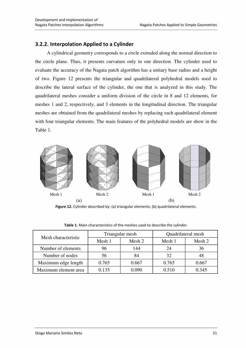
of two. Figure 12 presents the triangular and quadrilateral polyhedral models used to
describe the lateral surface of the cylinder, the one that is analyzed in this study. The
quadrilateral meshes consider a uniform division of the circle in 8 and 12 elements, for
meshes 1 and 2, respectively, and 3 elements in the longitudinal direction. The triangular
meshes are obtained from the quadrilateral meshes by replacing each quadrilateral element
with four triangular elements. The main features of the polyhedral models are show in the
Table 1.
Mesh 1 Mesh 2 Mesh 1 Mesh 2
(a) (b)
Figure 12. Cylinder described by: (a) triangular elements; (b) quadrilateral elements.
Table 1. Main characteristics of the meshes used to describe the cylinder.
Mesh characteristic Triangular mesh Quadrilateral mesh
Mesh 1 Mesh 2 Mesh 1 Mesh 2
Number of elements 96 144 24 36
Number of nodes 56 84 32 48
Maximum edge length 0.765 0.667 0.765 0.667
Maximum element area 0.135 0.090 0.510 0.345

Development and Implementation of
Nagata Patches Applied to Simple Geometries Nagata Patches Interpolation Algorithms
22 Diogo Mariano Simões Neto
3.2.2.1. Triangular Patches
In this section the analysis is perform for the polyhedral models of Figure 12 (a).
Meshes 1 and 2 are compared in terms of radial and normal vector errors, in order to study
the influence of the mesh size in the interpolation error. Figure 13 presents the error
distributions obtained for both Nagata patch interpolations.
Radial error (δr) [%]
Mesh 1 Mesh 2
Normal vector error (δn) [º]
Mesh 1 Mesh 2
Figure 13. Radial and normal vector errors on the triangular patches for the cylindrical surface.
One of the characteristics observed for both models is that the radial error is always
positive, i.e. Nagata patches are always outside the cylindrical analytical surface. This was
also observed in the Nagata interpolation of the quarter-circle. The maximum radial error
always occurs in the middle of the edges perpendicular to the axial direction of the
cylinder, thus showing the same trend as the case of the circle interpolation. The maximum
error for mesh 1 is 0.314% while for the mesh 2 is only 0.060% (see Figure 13). The radial
error decreases with mesh refinement, i.e. by increasing the number of elements in the
curve direction of the cylinder. Note that the maximum radial error is independent of the
number of elements in the axial direction, since it occurs at the edges perpendicular to the
axial direction of the cylinder.
Development and Implementation of
Nagata Patches Interpolation Algorithms Nagata Patches Applied to Simple Geometries
Diogo Mariano Simões Neto 23
Figure 13 also presents the normal vector error distribution for both discretizations.
Here also the normal vector error attains its maximum at the element edges, perpendicular
to the axial direction of the cylinder, showing a similar trend to the circle interpolation,
with two maximum values for each patch (see Figure 9 (a)). The maximum error for the
mesh 1 is 1.10º while for the mesh 2 is 70% lower (0.25º) (see Figure 13).
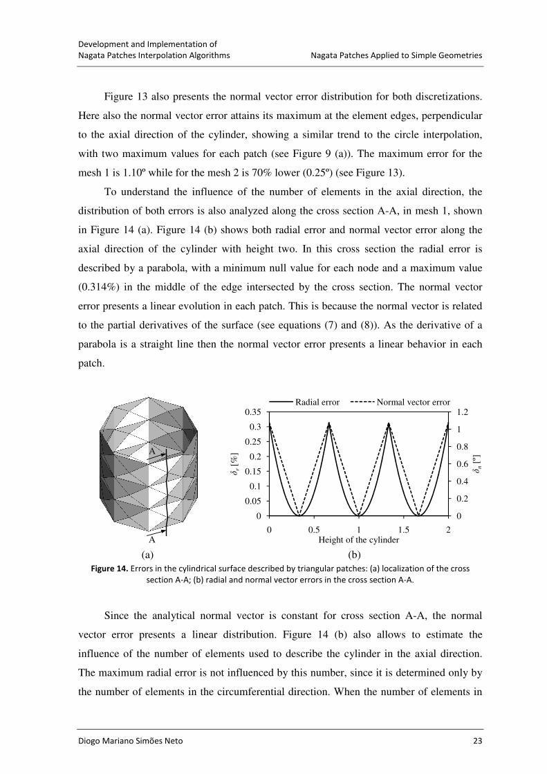
To understand the influence of the number of elements in the axial direction, the
distribution of both errors is also analyzed along the cross section A-A, in mesh 1, shown
in Figure 14 (a). Figure 14 (b) shows both radial error and normal vector error along the
axial direction of the cylinder with height two. In this cross section the radial error is
described by a parabola, with a minimum null value for each node and a maximum value
(0.314%) in the middle of the edge intersected by the cross section. The normal vector
error presents a linear evolution in each patch. This is because the normal vector is related
to the partial derivatives of the surface (see equations (7) and (8)). As the derivative of a
parabola is a straight line then the normal vector error presents a linear behavior in each
patch.
(a) (b)
Figure 14. Errors in the cylindrical surface described by triangular patches: (a) localization of the cross
section A-A; (b) radial and normal vector errors in the cross section A-A.
Since the analytical normal vector is constant for cross section A-A, the normal
vector error presents a linear distribution. Figure 14 (b) also allows to estimate the
influence of the number of elements used to describe the cylinder in the axial direction.
The maximum radial error is not influenced by this number, since it is determined only by
the number of elements in the circumferential direction. When the number of elements in
A
A
0
0.2
0.4
0.6
0.8
1
1.2
0
0.05
0.1
0.15
0.2
0.25
0.3
0.35
0 0.5 1 1.5 2
δn
[º]
δr[%
]
Height of the cylinder
Radial error Normal vector error

Development and Implementation of
Nagata Patches Applied to Simple Geometries Nagata Patches Interpolation Algorithms
24 Diogo Mariano Simões Neto
the axial direction decreases, the parabolic function describing the radial error widens
along the height of the cylinder (maintaining the maximum and minimum values). Since
the parabola widens, the maximum derivative decreases and, therefore, the maximum
normal vector error also decreases. This is shown in Figure 15, where the results for the
cross section A-A, with only 2 elements in the axial direction, are shown. These are the
reasons why, in this case, it was conclude that with the decrease in the number of elements
in the axial direction, the normal vector error decreases.
(a) (b)
Figure 15. Errors in the cylindrical surface described by 2 elements in axial direction: (a) localization of the
cross section A-A; (b) radial and normal vector errors in the cross section A-A.
3.2.2.2. Quadrilateral Patches
In this section, the error of the Nagata patch interpolation with quadrilateral elements
is analyzed. Both quadrilateral element meshes shown in Figure 12 (b) are studied. Figure
17 presents the error distributions obtained for both Nagata patch interpolations. Due to the
mesh symmetry in the axial direction, both the radial and the normal vector error present
the same distribution in any cross section to the cylinder axis. Therefore, only a cross
section is analyzed, since all other cross sections present the same behavior. This cross
section corresponds to the arc of circle, already analyzed in section 3.1.1. Notice that mesh
1 corresponds to the division of the arc of the circle studied in section 3.1.1 with 2
elements (normalized edge length of 0.78) and mesh 2 with 3 (normalized edge length of
0.52).
For the lateral cylindrical surface described by quadrilateral patches, the maximum
radial error in the mesh 1 and 2 is 0.314% and 0.060%, respectively, as show in Figure 16.
The maximum normal vector error is 0.703º and 0.202º for the meshes 1 and 2,
0
0.2
0.4
0.6
0.8
1
1.2
0
0.05
0.1
0.15
0.2
0.25
0.3
0.35
0 0.5 1 1.5 2
δn
[º]
δr[%
]
Height of the cylinder
Radial error Normal vector error

Development and Implementation of
Nagata Patches Interpolation Algorithms Nagata Patches Applied to Simple Geometries
Diogo Mariano Simões Neto 25
respectively. Figure 8 and Figure 9 with Figure 16 indicates that the radial error and the
normal vector error distributions are the same in the arc of a circle and any cross section to
the cylinder axis, when this is described by quadrilateral elements. Thus, as expected,
when using quadrilateral patches to describe the cylinder the number of elements along the
axial direction presents no influence in the approximation. The order of convergence to the
analytical cylindrical surface is dictated only by the mesh description in the circumferential
direction and is the same of the arc of a circle. As shown in Nagata (2005, 2010) the order
of convergence is quartic.
Radial error (δr) [%]
Mesh 1 Mesh 2
Normal vector error (δn) [º]
Mesh 1 Mesh 2
Figure 16. Radial and normal vector error on the quadrilateral patches for the cylindrical surface.
3.2.2.3. Comparison between Triangular and Quadrilateral Patches
In order to compare the triangular and quadrilateral Nagata patch interpolation, error
histograms were calculated for mesh 1, using the error values determined at each grid
point. The radial error histogram obtained for the triangular and quadrilateral patches is
presented in Figure 17 (a). It is clear that, although the maximum radial error is the same,
the distribution is different for the two types of patches. While the cylinder described by
triangular patches has about 80% of their points with a radial error of less than 0.01%, the
model described by quadrilateral patches has only 34% of their points with this range of

Development and Implementation of
Nagata Patches Applied to Simple Geometries Nagata Patches Interpolation Algorithms
26 Diogo Mariano Simões Neto
error. This difference is due to the higher number of nodes present in the triangular mesh
compared with the quadrilateral mesh (see Table 1), which leads to more information for
the Nagata patch algorithm. Thus, it seems that a parameter like the maximum element
area would be more appropriate for comparing the discretizations.
The normal vector error presents a different behavior. Although the maximum value
of the normal vector error is higher for the triangular patches, the average value is lower.
While the cylinder described by triangular patches has about 50% of its points with a
normal vector error less than 0.1º, the model described by quadrilateral patches has only
9% of its points within this error range (see Figure 17 (b)).
(a) (b)
Figure 17. Comparison between triangular and quadrilateral patches for the mesh 1 of the cylinder: (a)
radial error; (b) normal vector error.
3.2.3. Interpolation Applied to a Sphere
The first closed surface analyzed is the spherical geometry, where the sphere used to
evaluate the accuracy of the Nagata patch algorithm has unit radius. The construction of
structured quadrilateral meshes on the sphere geometry requires the division of the
triangular surfaces, which define each eighth, in three surfaces, each one with four sides.
This adds additional constrains to the mesh generation. Thus, mesh 1 is characterized, in
both polyhedral models, by presenting 2 elements along each quarter arc circle. Mesh 2
presents 3 elements along this arc, when using triangular elements. However, when using
quadrilateral elements an even number is mandatory. Thus, in that case, mesh 2 presents 4
elements. Although, these results in different maximum edge length, for mesh 1 and 2, the
maximum element area is similar for triangular and quadrilateral models.
0
10
20
30
40
50
60
70
80
90
100
0
0.0
3
0.0
6
0.0
9
0.1
2
0.1
5
0.1
8
0.2
1
0.2
4
0.2
7
0.3
Cum
ula
tive
num
ber
of
gri
d
po
ints
[%
]
δr [%]
Triangular patches
Quadrilateral patches
0
10
20
30
40
50
60
70
80
90
100
0
0.1
0.2
0.3
0.4
0.5
0.6
0.7
0.8
0.9 1
1.1
Cum
ula
tive
num
ber
of
gri
d
po
ints
[%
]
δn [º]
Triangular patches
Quadrilateral patches

Development and Implementation of
Nagata Patches Interpolation Algorithms Nagata Patches Applied to Simple Geometries
Diogo Mariano Simões Neto 27
Figure 18 presents the triangular and quadrilateral polyhedral models used to
describe the spherical surface. Both meshes are symmetrical relatively to the three
orthogonal cross sections of the sphere. The main features of the polyhedral models are
show in the Table 2.
Mesh 1 Mesh 2 Mesh 1 Mesh 2
(a) (b)
Figure 18. Sphere described by: (a) triangular elements; (b) quadrilateral elements.
Table 2. Main characteristics of the meshes used to describe the sphere.
Mesh characteristic Triangular mesh Quadrilateral mesh
Mesh 1 Mesh 2 Mesh 1 Mesh 2
Number of elements 32 72 24 96
Number of nodes 18 38 26 98
Maximum edge length 1.00 0.707 0.765 0.390
Maximum element area 0.433 0.194 0.461 0.145
3.2.3.1. Triangular Patches
To study the influence of the mesh size in the Nagata patch algorithm, the radial and
normal vector errors distributions, obtained for the models presented in Figure 18 (a) are
shown in Figure 19.
The maximum value of both errors (radial and normal vector) always occurs in the
middle of the edge with highest length, regardless of its orientation, since the sphere
presents the same curvature in all points. The analysis of Figure 19 indicates that the
normal vector error presents the same distribution as the radial error, reaching the
maximum value in the same locations.
Mesh 1 has a maximum radial error of 1.03% and a minimum of -0.21%, while the
range of the radial error for mesh 2 is only from -0.01% to 0.22%. These radial error
ranges can be observed in Figure 20 (a), which presents the error histogram, calculated

Development and Implementation of
Nagata Patches Applied to Simple Geometries Nagata Patches Interpolation Algorithms
28 Diogo Mariano Simões Neto
using the error values determined for each grid point. It is possible to observe that,
although the error range diminishes, both meshes present a similar distribution. Figure 20
(b) presents the normal vector error histogram, where it is possible to observe that the
maximum error value obtained for the mesh 1 and 2 are 5.1º and 1.5º, respectively. Both
the radial and normal vector errors decrease with the increase of the number of elements,
i.e. with the decrease of the maximum edge length.
Radial error (δr) [%]
Mesh 1 Mesh 2
Normal vector error (δn) [º]
Mesh 1 Mesh 2
Figure 19. Nagata patch error distributions for the sphere described by triangular elements.
(a) (b)
Figure 20. Error distribution in the sphere described by triangular elements: (a) radial error; (b) normal
vector error.
0
10
20
30
40
50
60
70
80
90
100
-0.2
-0.1 0
0.1
0.2
0.3
0.4
0.5
0.6
0.7
0.8
0.9 1
Cum
ula
tive
num
ber
of
gri
d
po
ints
[%
]
δr [%]
Mesh 1
Mesh 2
0
10
20
30
40
50
60
70
80
90
100
0
0.4
0.8
1.2
1.6 2
2.4
2.8
3.2
3.6 4
4.4
4.8
Mo
re
Cum
ula
tive
num
ber
of
gri
d
po
ints
[%
]
δn [º]
Mesh 1
Mesh 2

Development and Implementation of
Nagata Patches Interpolation Algorithms Nagata Patches Applied to Simple Geometries
Diogo Mariano Simões Neto 29
Triangular Nagata patches can also be applied to describe the quadrilateral meshes
presented in Figure 18 (b), applying two patches to describe each quadrilateral element of
the mesh. The division of the quadrilateral element into two triangular elements was
performed always with the goal of minimizing the maximum edge length. Thus, the
division was made using the smallest diagonal of the quadrilateral element. Applying this
strategy to the quadrilateral models, mesh 1 is represented by 48 triangular patches and
mesh 2 by 192, which corresponds to the double of the quadrilateral elements indicated in
Table 2. The maximum edge length increases when compared with the one of the
quadrilateral model. However, the maximum element area is half the value indicated in
Table 2 for the quadrilateral models.
The errors distributions are shown in Figure 21, for mesh 1 and 2, respectively. The
maximum value of both errors always occurs on the “virtual” edge, which is the one with
higher length and the radial error is mostly positive. These results are consistent with the
ones obtained using triangular patches to describe triangular polynomial models. The
results indicate that the order of convergence to the analytical surface is dictated by the
maximum edge length, whatever the type of polynomial model used to interpolate
triangular Nagata patches.
[%] Radial error (δr) [%]
Mesh 1 Mesh 2
[º] Normal vector error (δn) [º]
Mesh 1 Mesh 2
Figure 21. Nagata patch error distributions on the triangular patch for the sphere discretized by
quadrilateral elements.

Development and Implementation of
Nagata Patches Applied to Simple Geometries Nagata Patches Interpolation Algorithms
30 Diogo Mariano Simões Neto
3.2.3.2. Quadrilateral Patches
In this section the analysis is performed for the polyhedral models of Figure 18 (b),
using quadrilateral Nagata patches to make the surface interpolation. The error
distributions obtained for the quadrilateral patches are shown in Figure 22, for the mesh 1
and 2.
[%] Radial error (δr) [%]
Mesh 1 Mesh 2
[º] Normal vector error (δn) [º]
Mesh 1 Mesh 2
Figure 22. Radial and normal vector errors on the quadrilateral patches when the sphere is described by
quadrilateral elements.
The analysis of Figure 22 indicates that the radial error, when applying quadrilateral
patches, always presents higher negative values than positive. The areas with negative
error are located in the central area of the patches, as shown in the same figure. In the same
figure it is observed that the positive radial error is located near the edges of the elements,
taking the maximum value in the middle of the edge with highest length. The normal
vector error has its maximum value in the region where the maximum radial error is
positive, showing the same type of distribution as the sphere described with triangular
elements. In fact, the normal vector error distribution presents a similar range for the
models described with triangular or quadrilateral patches. This seems to indicate that this
error is mainly dictated by the maximum edge length, or the number of nodes. However,

Development and Implementation of
Nagata Patches Interpolation Algorithms Nagata Patches Applied to Simple Geometries
Diogo Mariano Simões Neto 31
unlike triangular patches, quadrilateral patches present a zone with a greater negative radial
error.
In order to better understand the difference between the two types of patches, the
following section presents a direct comparison between triangular and quadrilateral Nagata
patches.
3.2.3.3. Comparison between Triangular and Quadrilateral Patches
A direct comparison between triangular and quadrilateral patches was perform using
the quadrilateral models, mesh 1 and mesh 2, presented in Figure 18 (b). Figure 23 presents
the radial error distribution for mesh 1 (Figure 23 (a)) and mesh 2 (Figure 23 (b)). For both
polyhedral models, the modulus of the maximum radial error tends to be slightly higher for
the triangular interpolation. For quadrilateral interpolations the radial error tends to be
negative, while for triangular interpolations this error tends to be positive. This means that
triangular interpolations tend to describe a surface exterior to the sphere while quadrilateral
interpolations describe a more interior surface. For both polyhedral models, the radial error
distribution is narrower for triangular interpolations than for quadrilateral interpolations,
since for quadrilateral interpolations the radial error distribution is more uniform over the
Nagata patches [Neto et al., 2010a].
(a) (b)
Figure 23. Radial error distribution for the spherical surface discretized with quadrilateral elements: (a)
mesh 1; (b) mesh 2.
The comparison of Figure 21 and Figure 22 indicates that the normal vector error
distributions are different for both approaches. To analyze these differences, Figure 24
presents the normal vector error distribution for mesh 1 (Figure 24 (a)) and mesh 2 (Figure
0
5
10
15
20
25
30
35
40
45
-0.6
-0.5
-0.4
-0.3
-0.2
-0.1 0
0.1
0.2
0.3
0.4
0.5
0.6
Mo
re
Num
ber
of
gri
d p
oin
ts [
%]
δr [%]
Quadrilateral
patches
Triangular
patches
0
10
20
30
40
50
60
70
-0.0
6
-0.0
5
-0.0
4
-0.0
3
-0.0
2
-0.0
1 0
0.0
1
0.0
2
0.0
3
0.0
4
0.0
5
0.0
6
Mo
re
Num
ber
of
gri
d p
oin
s [%
]
δr [%]
Quadrilateral
patches
Triangular
patches

Development and Implementation of
Nagata Patches Applied to Simple Geometries Nagata Patches Interpolation Algorithms
32 Diogo Mariano Simões Neto
24 (b)). For both polyhedral models, the distribution presents a lower average value for
triangular interpolations. Thus, the normal vector error distribution is more uniform over
the quadrilateral Nagata patches.
This comparison seems to indicate that the normal vector error is mainly dictated by
the number of nodes, whatever the type of Nagata patches used. The geometrical error,
evaluated using the radial error, depends on the type of Nagata patch used. In case of this
closed surface with constant curvature, quadrilateral patches interpolation is closer to the
polynomial model, presenting a radial error that tends to be negative, while triangular
patches interpolations presents a more positive trend.
(a) (b)
Figure 24. Normal vector error distribution for the spherical surface discretized with quadrilateral elements:
(a) mesh 1; (b) mesh 2.
3.2.4. Interpolation Applied to a Torus
The second closed surface used to evaluate the accuracy of the Nagata patch
algorithm is a torus, with major and minor radii of 2R = and 1r = , respectively. The ring
torus ( R r> ) is characterized by having regions of elliptic, parabolic, and hyperbolic
points, which make it more complex than the sphere. Figure 25 presents the triangular and
quadrilateral polyhedral models used to describe the torus surface. Both quadrilateral
meshes consider a uniform division of the circle entered in the minor and major radius
cross section of the torus in 8 and 12 elements, for the meshes 1 and 2, respectively. The
triangular meshes are obtained from the quadrilateral meshes by replacing each
quadrilateral element with four triangular elements. The main features of the polyhedral
models are show in Table 3.
0
5
10
15
20
25
30
0
0.3
0.6
0.9
1.2
1.5
1.8
2.1
2.4
2.7 3
Mo
re
Num
ber
of
gri
d p
oin
ts [
%]
δn [º]
Quadrilateral
patches
Triangular
patches
0
5
10
15
20
25
30
35
0
0.0
6
0.1
2
0.1
8
0.2
4
0.3
0.3
6
0.4
2
0.4
8
0.5
4
Mo
re
Num
ber
of
gri
d p
oin
ts [
%]
δn [º]
Quadrilateral
patches
Triangular
patches
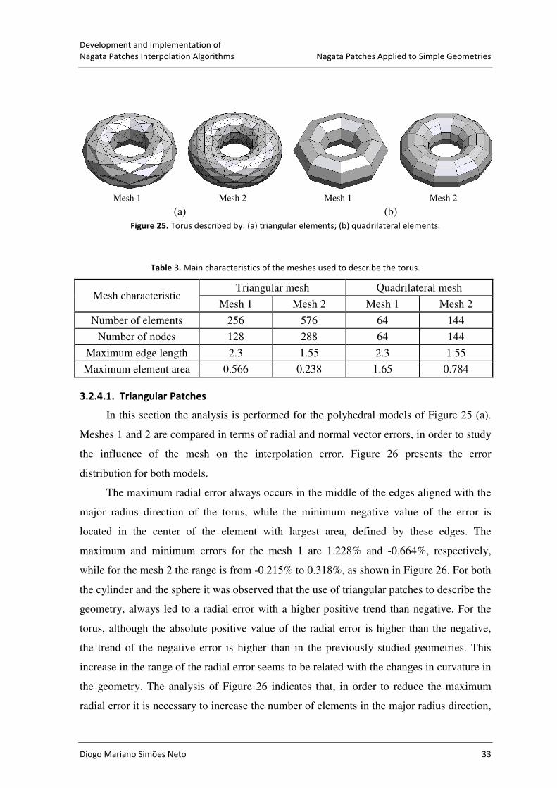
Development and Implementation of
Nagata Patches Interpolation Algorithms Nagata Patches Applied to Simple Geometries
Diogo Mariano Simões Neto 33
Mesh 1 Mesh 2 Mesh 1 Mesh 2
(a) (b)
Figure 25. Torus described by: (a) triangular elements; (b) quadrilateral elements.
Table 3. Main characteristics of the meshes used to describe the torus.
Mesh characteristic Triangular mesh Quadrilateral mesh
Mesh 1 Mesh 2 Mesh 1 Mesh 2
Number of elements 256 576 64 144
Number of nodes 128 288 64 144
Maximum edge length 2.3 1.55 2.3 1.55
Maximum element area 0.566 0.238 1.65 0.784
3.2.4.1. Triangular Patches
In this section the analysis is performed for the polyhedral models of Figure 25 (a).
Meshes 1 and 2 are compared in terms of radial and normal vector errors, in order to study
the influence of the mesh on the interpolation error. Figure 26 presents the error
distribution for both models.
The maximum radial error always occurs in the middle of the edges aligned with the
major radius direction of the torus, while the minimum negative value of the error is
located in the center of the element with largest area, defined by these edges. The
maximum and minimum errors for the mesh 1 are 1.228% and -0.664%, respectively,
while for the mesh 2 the range is from -0.215% to 0.318%, as shown in Figure 26. For both
the cylinder and the sphere it was observed that the use of triangular patches to describe the
geometry, always led to a radial error with a higher positive trend than negative. For the
torus, although the absolute positive value of the radial error is higher than the negative,
the trend of the negative error is higher than in the previously studied geometries. This
increase in the range of the radial error seems to be related with the changes in curvature in
the geometry. The analysis of Figure 26 indicates that, in order to reduce the maximum
radial error it is necessary to increase the number of elements in the major radius direction,

Development and Implementation of
Nagata Patches Applied to Simple Geometries Nagata Patches Interpolation Algorithms
34 Diogo Mariano Simões Neto
i.e. larger number of divisions of the circle corresponding to the major radius cross section
of the torus.
Also, the normal vector error attains its maximum in the elements that contain edges
aligned with the major radius direction, as shown in Figure 26. The maximum error for
mesh 1 is 9.6º while for mesh 2 is 3.9º. However, it is important to mention that 50% of the
elements have an error below 1º and 0.3º for mesh 1 and 2, respectively. The analysis of
the radial and normal vector error distributions indicates that, in order to reduce the
extreme values of error, the mesh must have more elements in the major radius direction.
This will distribute the error more uniformly over the Nagata patches.
[%] Radial error (δr) [%]
Mesh 1 Mesh 2
[º] Normal vector error (δn) [º]
Mesh 1 Mesh 2
Figure 26. Radial and normal vector errors on the triangular patches used to describe the torus.
3.2.4.2. Quadrilateral Patches
In this section, the error associated to Nagata patch interpolation of the torus
discretized with quadrilateral elements is analyzed. Both quadrilateral element meshes,
shown in Figure 25 (b), are studied. Figure 27 shows the radial and normal vector error
distributions on the quadrilateral patches, for mesh 1 and 2, respectively.
For mesh 1 the radial error range is from -2.42% to 2.36% while for the mesh 2 the
range is only from -0.547% to 0.522%, as shown in Figure 27. For both meshes, the
patches with negative error are located in the region far from the axis of the torus, where

Development and Implementation of
Nagata Patches Interpolation Algorithms Nagata Patches Applied to Simple Geometries
Diogo Mariano Simões Neto 35
the geometry is concave in all directions. These results are consistent with the ones
obtained for the sphere, which is also concave in all directions. The maximum (positive)
radial error is located in the region where the principal curvatures have opposite signs, i.e.
at hyperbolic points.
The normal vector error reaches its maximum value at the edges with higher length,
of elements with negative radial error, as observed in Figure 27. The maximum value is
9.1º and 3.1º for meshes 1 and 2, respectively. Mesh 1 presents an error less than 4.55º and
mesh 2 of 1.55º, in all hyperbolic points of the torus surface, i.e. half the maximum value.
The analysis of the figure indicates that the normal vector error attains its maximum value
in the region where the radial error alters from positive to negative, where the surface is
elliptic and the edge length is higher. It is interesting to notice that, for the torus, the
normal vector error range for triangular and quadrilateral patches is similar, being slightly
higher for the triangular patches. However, its distribution is quite different. Thus, in order
to analyze the distributions, in the following section a comparison between all meshes,
used to represent the torus surface with Nagata patches, is performed.
[%] Radial error (δr) [%]
Mesh 1 Mesh 2
[º] Normal vector error (δn) [º]
Mesh 1 Mesh 2
Figure 27. Radial and normal vector errors on the quadrilateral patches used to describe the torus.

Development and Implementation of
Nagata Patches Applied to Simple Geometries Nagata Patches Interpolation Algorithms
36 Diogo Mariano Simões Neto
3.2.4.3. Comparison between Triangular and Quadrilateral Patches
All the polyhedral models shown in Figure 25, applied to describe the torus, were
used to perform a comparison between triangular and quadrilateral patches. Figure 28
presents the radial error distribution in all meshes used to describe the torus surface,
calculated using the error values determined at each grid point. It is observed that mesh 1,
with the application of quadrilateral Nagata patches, is clearly the worst approximation due
to the smaller number of nodes used in the discretization of the model (cf. Table 3), and
therefore less information is available for the Nagata interpolation algorithm. Except for
this model, the remaining interpolations present more than 90% of their grid points with an
error range of less than 1%.
Figure 28. Radial error distribution on the Nagata patches used to describe the torus surface.
The maximum normal vector error tends to be slightly higher for triangular meshes
in comparison with quadrilateral meshes, as observed in Figure 27. In order to highlight the
differences, Figure 29 presents the normal vector error, cumulative distribution, for all
meshes used to describe the torus surface. It is observed that, although the triangular
meshes have two times more nodes than the quadrilateral meshes, the maximum error is
approximately the same. The worst approximations are always obtained with mesh 1, for
which the quadrilateral Nagata patches present a more uniform error distribution. The
increase in the number of nodes clearly increases the amount of grid points with a lower
normal vector error. Both mesh 2 models, present more than 90% of their grid points with
an error less than 1%. However, for triangular patches, approximately 50% of the grid
0
10
20
30
40
50
60
70
80
90
100
-2.4
-2.2
-2.0
-1.8
-1.6
-1.4
-1.2
-1.0
-0.8
-0.6
-0.4
-0.2
0.0
0.2
0.4
0.6
0.8
1.0
1.2
1.4
1.6
1.8
2.0
2.2
Mo
re
Cum
ula
tive
num
ber
of
gri
d
po
ints
[%
]
δr [%]
Triangular patches - Mesh 1
Triangular patches - Mesh 2
Quadrilateral patches - Mesh 1
Quadrilateral patches - Mesh 2

Development and Implementation of
Nagata Patches Interpolation Algorithms Nagata Patches Applied to Simple Geometries
Diogo Mariano Simões Neto 37
points have an error inferior to 0.2% while, for quadrilateral patches, only 7.5% of the grid
points present that error range.
Figure 29. Normal vector error distribution on the Nagata patches used to describe the torus surface.
0
10
20
30
40
50
60
70
80
90
100
0
0.4
0.8
1.2
1.6 2
2.4
2.8
3.2
3.6 4
4.4
4.8
5.2
5.6 6
6.4
6.8
7.2
7.6 8
8.4
8.8
9.2
Cum
ula
tive
num
ber
of
gri
d
po
ints
[%
]
δn [º]
Triangular patches - Mesh 1
Triangular patches - Mesh 2
Quadrilateral patches - Mesh 1
Quadrilateral patches - Mesh 2

Development and Implementation of
Vertex Normal Vector Estimative Nagata Patches Interpolation Algorithms
38 Diogo Mariano Simões Neto
4. VERTEX NORMAL VECTOR ESTIMATIVE
Typically, when a surface is approximated by a polyhedral mesh, only the vertex
positions are known. However, the Nagata interpolation algorithm requires the knowledge
of the normal vector for each vertex (node), as highlighted in equation (3). Thus, it is
important to develop a strategy that allows for vertex normal vector estimative, based on
the information available in the polyhedral model. In this section some algorithms for
approximation of vertex normal vector are presented and analyzed.
4.1. Vertex Normal Algorithms
The vertex normal vector is typically taken as a weighted sum of the normal vectors
of the planes defined by the reciprocal edges of the vertex. If n edges of the polyhedral
mesh are defined with vertex j , the estimative of the normal vector of vertex j involves
the determination of the normal vector, n , for each of the n planes. Figure 30 presents the
notation used to define the reciprocal edges as well as the normal vectors of each plane,
when evaluating the normal vector of vertex j .
The methods presented in this section differ substantially from each other, but they
all share the notion of weighting adjacent elements normal vectors [Jin et al., 2005].
Figure 30. Notation used to calculate the normal vector at vertex j .
1n
2
n–1
...
j
k
k+1
k+2
k+n–1
k+n–2
nn
n1
n2
nn–1
n...

Development and Implementation of
Nagata Patches Interpolation Algorithms Vertex Normal Vector Estimative
Diogo Mariano Simões Neto 39
4.1.1. Mean Weighted Equally
The algorithm to estimate the vertex normal vector presented in this subsection was
introduced by H. Gouraud, in 1971. This algorithm will be referred to as the mean
weighted equally (MWE) algorithm, since the normal vector is determined as [Gouraud,
1971]:
MWE
1
,n
i
i=
∑n n� (20)
where in is the normal vector of the plane (element) i and the summation is over all the n
planes (elements) defined by vertex j (cf. Figure 30). The symbol � indicates that the
calculated vector is parallel to the vertex normal vector, since the normal vector is always
unitary.
4.1.2. Mean Weighted by Angle
While Gouraud (1971) suggested equal weights, in 1998 G. Thürmer and C.
Wüthrich proposed as weights the planes (elements) angles at the vertex. Defining as iα
the angle between the two edge vectors ie and 1i+e of plane (element) i sharing the vertex
(see Figure 30), the normal vector of the vertex is determined as [Thürmer and Wüthrich,
1998]:
MWA
1
.n
i i
i
α=
∑n n� (21)
This will be referred as the mean weighted by angle (MWA) algorithm.
4.1.3. Mean Weighted by Sine and Edge Length Reciprocals
The next four algorithms were introduced by N. Max, in 1999. The first algorithm,
referred as the mean weighted by sine and edge length reciprocals (MWSELR), takes into
account the differences in size of the adjacent edges to the vertex, assigning larger weights
to smaller edges and higher angles between the two edge vectors. The normal vector to the
vertex is determined as [Max, 1999]:
MWSELR
1 1
sin( ),
n
i i
i i i
α
= +
∑n
ne e
� (22)

Development and Implementation of
Vertex Normal Vector Estimative Nagata Patches Interpolation Algorithms
40 Diogo Mariano Simões Neto
where in ,
ie , 1i+e and iα as defined in the previous section.
4.1.4. Mean Weighted by Areas of Adjacent Triangles
The second algorithm, proposed by Max (1999), incorporates the area of the triangle
formed by the two edges of each plane (whether the element is triangular or not) incident
on the vertex. Thus, this algorithm assigns larger weights to elements with larger area. The
vertex normal vector is estimated using the following expression:
MWAAT 1 1
1 1
sin( ) ,n n
i i i i i i i
i i
α+ += =
= ⊗∑ ∑n n e e n e e� (23)
where in ,
ie , 1i+e and iα were defined in section 4.1.2 and ⊗ represents the cross product
of two vectors. This algorithm will be referred as the mean weighted by areas of adjacent
triangles (MWAAT).
4.1.5. Mean Weighted by Edge Length Reciprocals
Max (1999) also proposes to remove the sine factor in equation (22), which leads to
an estimate of the vertex normal vector given as:
MWELR
1 1
,n
i
i i i= +
∑n
ne e
� (24)
where in ,
ie , 1i+e are defined as in equation (21). This algorithm will be referred as the
mean weighted by edge length reciprocals (MWELR) and assigns larger weights to smaller
edges.
4.1.6. Mean Weighted by Square Root of Edge Length Reciprocals
The last algorithm proposed by Max (1999) is similar to the MWELR, with the
addition of a square root:
MWRELR
1 1
,n
i
ii i
= +
∑n
ne e
� (25)
where in ,
ie , 1i+e are defined as in equation (21). This will be referred as the mean
weighted by square root of edge length reciprocals (MWRELR) algorithm.

Development and Implementation of
Nagata Patches Interpolation Algorithms Vertex Normal Vector Estimative
Diogo Mariano Simões Neto 41
4.2. Algorithms Applied to Simple Geometries
In order to evaluate the efficiency of the vertex normal vector estimate algorithms
presented in the previous section, they were applied to the simple geometries used in the
previous chapter. The geometries chosen are the cylinder, as an open surface, and the
sphere and the torus, as closed surfaces. Both triangular and quadrilateral polyhedral
descriptions are used and compared in this analysis. For both models, the normal vector
approximation algorithms are applied for each node, and the error in the normal vector
approximation is evaluated. This error is determined, for each node of the mesh, using the
following definition:
1
analytical algorithmiccos ( ) [º ],θ −= ⋅n n (26)
where algorithmicn is the unit normal vector, evaluated using the different algorithms
previously presented, and analyticaln is the unit normal vector to the surface, evaluated using
the analytical function. Thus, this error calculated only in the nodes of the mesh,
corresponds to the angular difference between the analytical and the approximated normal
vectors, expressed in degrees.
4.2.1. Algorithms Applied to the Cylinder
Both polyhedral models shown in Figure 12 are used to evaluate the efficiency of the
algorithms. The models with quadrilateral elements, shown in Figure 12 (b), present the
same characteristic of having elements that share the same node arranged symmetrically
and all of them with the same dimensions and shape. Therefore, all the algorithms will lead
to the same normal vector estimative, at each node, which is equal to the analytical normal
vector value. For these reasons this results are not presented here.
The triangular meshes presented in Figure 12 (a) have elements with different shapes
and areas. The nodes are shared by a different number of elements, depending on their
position in the mesh. The error in the normal vector approximation, obtained using the
various algorithms applied to mesh 2, is shown in Figure 31. For all approaches, the
maximum error is always located on the boundaries of the cylinder geometry, where the
nodes are shared by fewer elements. Except for the boundary nodes, the normal vector
approximation error is less that 0.6º.

Development and Implementation of
Vertex Normal Vector Estimative Nagata Patches Interpolation Algorithms
42 Diogo Mariano Simões Neto
θ [º]
MWE MWA MWSELR
MWAAT MWELR MWRELR
Figure 31. Normal vector approximation error attained for each algorithm applied to mesh 2 of the cylinder.
Figure 32 presents the maximum normal vector approximation error for both
triangular meshes (mesh 1 and mesh 2) of the cylinder. In both meshes the maximum error
occurs in the boundary nodes such as show in Figure 31.
Figure 32. Maximum normal vector approximation error for the various algorithms applied to the cylinder
described with triangular elements.
The analysis of Figure 32 indicates that all algorithms give, approximately, the same
maximum normal vector error in the nodes of the boundary and that the error is higher
when compared with the one obtained for the interior nodes. Thus, the use of this open
0
1
2
3
4
5
6
7
MWE MWA MWSELR MWAAT MWELR MWRELR
Max
imum
θ[º
]
Mesh 1
Mesh 2

Development and Implementation of
Nagata Patches Interpolation Algorithms Vertex Normal Vector Estimative
Diogo Mariano Simões Neto 43
surface (lateral surface of the cylinder) highlights the difficulty to obtain good
approximations for nodes located on the boundaries.
4.2.2. Algorithms Applied to the Sphere
All polyhedral models of the sphere, shown in Figure 18, are used to compare the
normal vector approximation algorithms. For both triangular and quadrilateral polyhedral
models, mesh 1 presents complete symmetry of elements arrangement, as shown in Figure
18. Each node of these meshes is shared by a set of elements symmetrically distributed
and, consequently, all the algorithms give a normal vector approximation equal to the
analytical normal vector value. Therefore, these two meshes correspond to a particular
case, and their results are not shown here.
The normal vector algorithms were applied to mesh 2 polyhedral models and the
normal vector approximation error was determined, for each node. The results are shown
in Figure 33 and Figure 34, for triangular and quadrilateral meshes, respectively.
Figure 33 shows that, for the triangular mesh, the maximum error always occurs on
the same nodes, regardless of the algorithm used. Except for the MWA algorithm, the
quadrilateral mesh has the maximum error located always in the same nodes of the mesh,
as shown in Figure 34. The different results obtained with the MWA for triangular and
quadrilateral meshes can be related to the fact that, for the quadrilateral mesh the iα angle
is higher than for the triangular mesh and can be higher or lower than 90º. Therefore this
method seems to be more suitable for polyhedral descriptions with smaller angles (always
less than 90º). In both polyhedral models there are nodes with zero or very low error
values, corresponding to nodes that are shared by elements that have a symmetrical
distribution.
Figure 35 shows the maximum angular error between the analytical and the
approximated normal vector, attained for each algorithm. Globally, the triangular mesh
description leads to higher error values, except for the MWA. The MWSELR algorithm
leads a zero error for both types of polyhedral descriptions, which is probably due to the
fact that the edges size and angle present inverse weights in equation (22) [Neto et al.,
2010b]. In fact, since both models were built using a structured mesh generation algorithm
the MWAAT, MWELR and MWRELR present similar results to the MWE.
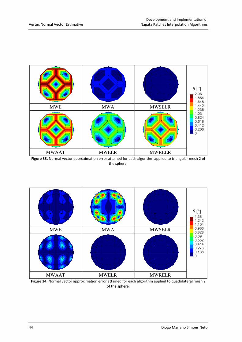
Development and Implementation of
Vertex Normal Vector Estimative Nagata Patches Interpolation Algorithms
44 Diogo Mariano Simões Neto
θ [º]
MWE MWA MWSELR
MWAAT MWELR MWRELR
Figure 33. Normal vector approximation error attained for each algorithm applied to triangular mesh 2 of
the sphere.
θ [º]
MWE MWA MWSELR
MWAAT MWELR MWRELR
Figure 34. Normal vector approximation error attained for each algorithm applied to quadrilateral mesh 2
of the sphere.

Development and Implementation of
Nagata Patches Interpolation Algorithms Vertex Normal Vector Estimative
Diogo Mariano Simões Neto 45
Figure 35. Maximum normal vector approximation error for the various algorithms applied to the sphere.
4.2.3. Algorithms Applied to the Torus
All the polyhedral models of the torus, presented in Figure 25, are used to analyze
the normal vector approximation algorithms. The normal vector approximation error
distributions, obtained with each algorithm are shown in Figure 36 and Figure 37, for mesh
1 of triangular and quadrilateral polyhedral models, respectively.
For the triangular mesh, all algorithms present a similar normal vector error
distribution, except the MWA and MWSELR. The maximum error values are located near
the place where the change of concave to convex curvature occurs, as shown in Figure 36.
When the MWSELR algorithm is applied, the maximum error value occurs for a small
number of nodes located inside the torus. Also, it rapidly decreases for the remainder
nodes.
θ [º]
MWE MWA MWSELR
MWAAT MWELR MWRELR
Figure 36. Normal vector approximation error attained for each algorithm applied to triangular mesh of the
torus (mesh 1).
0
0.5
1
1.5
2
2.5
MWE MWA MWSELR MWAAT MWELR MWRELR
Max
imum
θ[º
]
Triangular Patches
Quadrilateral Patches

Development and Implementation of
Vertex Normal Vector Estimative Nagata Patches Interpolation Algorithms
46 Diogo Mariano Simões Neto
θ [º]
MWE MWA MWSELR
MWAAT MWELR MWRELR
Figure 37. Normal vector approximation error attained for each algorithm applied to quadrilateral mesh of
the torus (mesh 1).
For quadrilateral elements all algorithms give a small value of error (less that 0.7º),
except the MWA algorithm, which attains a maximum of about 5.5º, as shown in Figure
37. As already mentioned, this algorithm is not adequate for meshes that contain elements
with angles both higher and lower that 90º (quadrilateral elements). This result is more
perceptible for nodes shared by elements with a higher difference in their angle values.
(a) (b)
Figure 38. Maximum normal vector approximation error for the various algorithms applied to the torus: (a)
triangular mesh; (b) quadrilateral mesh.
Figure 38 presents the maximum normal vector approximation error, for the different
algorithms, applied to the polyhedral descriptions presented in Figure 25. Although, the
triangular mesh has more nodes than the quadrilateral, and therefore more information, the
0
2
4
6
8
10
12
Max
imum
θ[º
]
Mesh 1
Mesh 2
0
2
4
6
8
10
12
Max
imum
θ[º
]
Mesh 1
Mesh 2
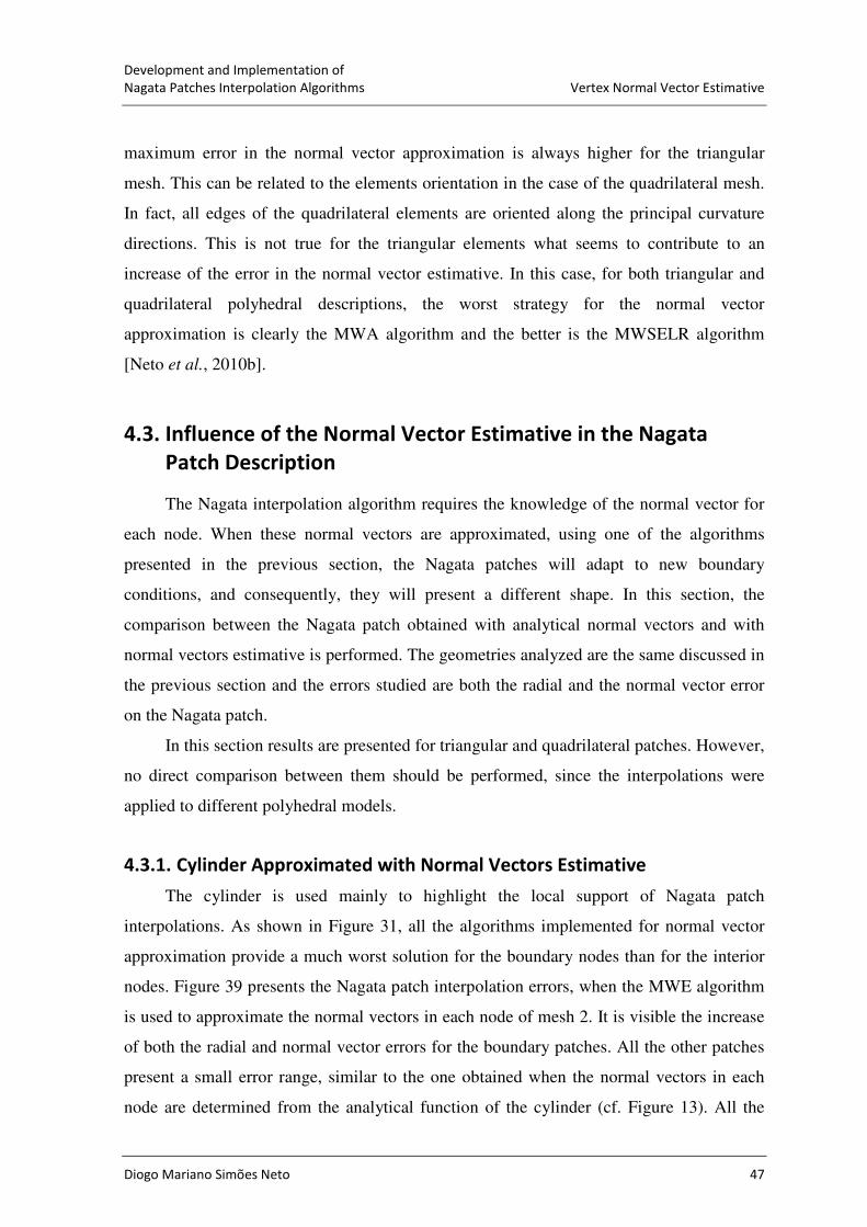
Development and Implementation of
Nagata Patches Interpolation Algorithms Vertex Normal Vector Estimative
Diogo Mariano Simões Neto 47
maximum error in the normal vector approximation is always higher for the triangular
mesh. This can be related to the elements orientation in the case of the quadrilateral mesh.
In fact, all edges of the quadrilateral elements are oriented along the principal curvature
directions. This is not true for the triangular elements what seems to contribute to an
increase of the error in the normal vector estimative. In this case, for both triangular and
quadrilateral polyhedral descriptions, the worst strategy for the normal vector
approximation is clearly the MWA algorithm and the better is the MWSELR algorithm
[Neto et al., 2010b].
4.3. Influence of the Normal Vector Estimative in the Nagata
Patch Description
The Nagata interpolation algorithm requires the knowledge of the normal vector for
each node. When these normal vectors are approximated, using one of the algorithms
presented in the previous section, the Nagata patches will adapt to new boundary
conditions, and consequently, they will present a different shape. In this section, the
comparison between the Nagata patch obtained with analytical normal vectors and with
normal vectors estimative is performed. The geometries analyzed are the same discussed in
the previous section and the errors studied are both the radial and the normal vector error
on the Nagata patch.
In this section results are presented for triangular and quadrilateral patches. However,
no direct comparison between them should be performed, since the interpolations were
applied to different polyhedral models.
4.3.1. Cylinder Approximated with Normal Vectors Estimative
The cylinder is used mainly to highlight the local support of Nagata patch
interpolations. As shown in Figure 31, all the algorithms implemented for normal vector
approximation provide a much worst solution for the boundary nodes than for the interior
nodes. Figure 39 presents the Nagata patch interpolation errors, when the MWE algorithm
is used to approximate the normal vectors in each node of mesh 2. It is visible the increase
of both the radial and normal vector errors for the boundary patches. All the other patches
present a small error range, similar to the one obtained when the normal vectors in each
node are determined from the analytical function of the cylinder (cf. Figure 13). All the

Development and Implementation of
Vertex Normal Vector Estimative Nagata Patches Interpolation Algorithms
48 Diogo Mariano Simões Neto
other implemented algorithms for normal vector estimative produce a similar distribution
for the other Nagata interpolation error values. Thus, the Nagata patches follow the same
behavior as the normal vector approximation, i.e. a good approximation at the interior
patches and a solution not so good at the boundary patches.
[%] Radial error (δr) Normal vector error (δn) [º]
Figure 39. Radial and normal vector errors on the triangular patches used to describe the cylinder (mesh 2)
when the MWE algorithm is used to estimate the normal vectors.
4.3.2. Sphere Approximated with Normal Vectors Estimative
In this section, only mesh 2 for both triangular and quadrilateral polyhedral
descriptions (see Figure 18) will be used to analyze the influence of the normal vectors in
the Nagata interpolation algorithm, since the other correspond to a particular case. The
Nagata patch interpolation was applied using the normal vectors estimative, obtained with
the different algorithms, and the results are compared with the ones obtained for the
Nagata patch interpolation using the analytically determined normal vectors (labeled
EXACT). Figure 40 presents both the radial and normal vector errors in the Nagata patch
interpolation, obtained when applying the MWA algorithm to approximate the normal
vectors in each node of the triangular mesh. The error distributions are similar to the ones
obtained with the analytical normal vector, previously presented in Figure 19.
[%] Radial error (δr) Normal vector error (δn) [º]
Figure 40. Radial and normal vector errors on the triangular patches used to describe the sphere (mesh 2)
when the MWA algorithm is used to estimate the normal vectors.
Development and Implementation of
Nagata Patches Interpolation Algorithms Vertex Normal Vector Estimative
Diogo Mariano Simões Neto 49
Figure 41 (a) and (b) shows the maximum and minimum radial error of the Nagata
patches interpolation, respectively, for both types of patches using analytical and
approximated normal vectors. The comparison of Figure 35 and Figure 41 indicates that
there is a direct relationship between both errors. However, the relationship between the
normal vector estimative error and the radial error is no linear.
Nonetheless, usually the increase in the normal vector approximation error implies
an increase in the radial error range. Only when the MWA algorithm is applied to estimate
the normal vectors, the Nagata triangular patch algorithm presents a smaller radial error
range than with the normal vectors provided by the analytical function, as shown in Figure
41. However, this corresponds to a particular case of interpolation, for which the radial
error diminishes due to the error introduced in the normal vector boundary conditions. It is
important to mention that all algorithms lead to a radial error range always inferior to 0.9%
in the triangular patches and 0.25% in the quadrilateral patches, although the polyhedral
meshes description used can be considered coarse.
(a) (b)
Figure 41. Nagata patch radial error in the sphere description (mesh 2) using different algorithms to
estimate the normal vector: (a) maximum; (b) minimum.
Figure 42 presents the maximum normal vector error at the Nagata patches using
different algorithms to estimate the normal vector in each node. The analysis of the figure
indicates that, when the normal vectors at the nodes of the mesh are approximate, the
normal vector error in the Nagata patch increases, presenting the same behavior of the
radial error. Thus, the increase in the normal vector approximation error (at the nodes)
implies an increase in the range of normal vector error. It is important to mention that,
0
0.1
0.2
0.3
0.4
0.5
0.6
Max
imum
δr
[%]
Triangular Patches Quadrilateral Patches-0.6
-0.5
-0.4
-0.3
-0.2
-0.1
0
Min
imum
δr [%
]
Triangular Patches Quadrilateral Patches
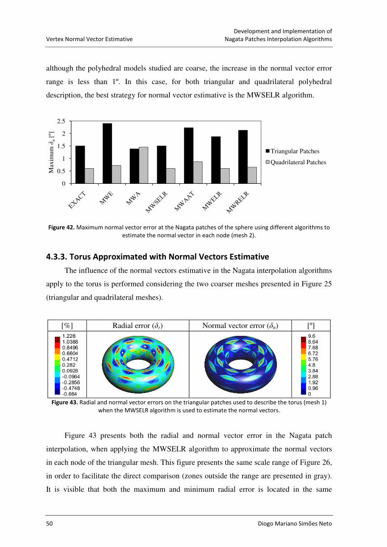
Development and Implementation of
Vertex Normal Vector Estimative Nagata Patches Interpolation Algorithms
50 Diogo Mariano Simões Neto
although the polyhedral models studied are coarse, the increase in the normal vector error
range is less than 1º. In this case, for both triangular and quadrilateral polyhedral
description, the best strategy for normal vector estimative is the MWSELR algorithm.
Figure 42. Maximum normal vector error at the Nagata patches of the sphere using different algorithms to
estimate the normal vector in each node (mesh 2).
4.3.3. Torus Approximated with Normal Vectors Estimative
The influence of the normal vectors estimative in the Nagata interpolation algorithms
apply to the torus is performed considering the two coarser meshes presented in Figure 25
(triangular and quadrilateral meshes).
[%] Radial error (δr) Normal vector error (δn) [º]
Figure 43. Radial and normal vector errors on the triangular patches used to describe the torus (mesh 1)
when the MWSELR algorithm is used to estimate the normal vectors.
Figure 43 presents both the radial and normal vector error in the Nagata patch
interpolation, when applying the MWSELR algorithm to approximate the normal vectors
in each node of the triangular mesh. This figure presents the same scale range of Figure 26,
in order to facilitate the direct comparison (zones outside the range are presented in gray).
It is visible that both the maximum and minimum radial error is located in the same
0
0.5
1
1.5
2
2.5
Max
imum
δn
[º]
Triangular Patches
Quadrilateral Patches

Development and Implementation of
Nagata Patches Interpolation Algorithms Vertex Normal Vector Estimative
Diogo Mariano Simões Neto 51
regions, when using the MWSELR algorithm and when the normal vectors are determined
using the analytical function. It is important to notice that, when the MWSELR algorithm
is used, the extreme values of radial error are located near the nodes where the error in the
normal vectors approximation is higher (see Figure 36). The normal vector error presents
also a similar distribution when using the analytical normal vector or the estimative
calculated with the MWSELR algorithm.
Figure 44 shows the maximum and minimum radial errors obtained for the Nagata
patches interpolation of the polyhedral description of the torus, for both triangular and
quadrilateral patches, using analytical (labeled EXACT) and approximated normal vectors.
The analysis of Figure 38 and Figure 44 indicates the increase of the normal vector
approximation error does not necessarily result in an increase of the radial error range, on
the contrary it may even decrease (see Figure 44). This effect is clear in case of the
MWELR and MWRELR algorithms, applied to triangular elements. In both cases, the
normal vector approximation error introduces changes in the boundary conditions, which
lead to a distribution of the radial error by several neighboring patches.
(a) (b)
Figure 44. Nagata patch radial error in the torus description (mesh 1) using different algorithms to estimate
the normal vector: (a) maximum; (b) minimum.
Figure 45 presents the maximum normal vector error at the Nagata patches
interpolation of the torus, for both triangular and quadrilateral patches, using different
algorithms to estimate the normal vector in each node. For triangular patches, the MWA
algorithm leads to the worst interpolation, due to the large error values in the normal
0
0.5
1
1.5
2
2.5
3
3.5
Max
imum
δr
[%]
Triangular Patches Quadrilateral Patches-3.5
-3
-2.5
-2
-1.5
-1
-0.5
0
Min
imum
δr [%
]
Triangular Patches Quadrilateral Patches

Development and Implementation of
Vertex Normal Vector Estimative Nagata Patches Interpolation Algorithms
52 Diogo Mariano Simões Neto
vectors and also to the fact that this error is highly concentrated in specific nodes (see
Figure 36).
Figure 45. Maximum normal vector error at the Nagata patches of the torus using different algorithms to
estimate the normal vector in each node (mesh 1).
For the torus geometry, the MWA algorithm leads to the worst Nagata patch
interpolation results, for both triangular and quadrilateral polyhedral descriptions, due to
the large error in the normal vectors approximation. All others algorithms give
approximately the same radial error range, for the case of quadrilateral patches. For
triangular patches this also occurs, exception made for the MWAAT.
The results presented in this section highlight the importance of analyzing the overall
distribution of the geometrical error of the Nagata patch interpolation. In fact, the analysis
of the normal vector error approximation is not sufficient to select the best approximation
algorithm. This selection is dictated also by the surface geometry and the polyhedral model
adopted.
0
5
10
15
20
25
30
35
40
Max
imum
δn
[º]
Triangular Patches
Quadrilateral Patches

Development and Implementation of
Nagata Patches Interpolation Algorithms Normal Vector Evaluated from CAD Geometry
Diogo Mariano Simões Neto 53
5. NORMAL VECTOR EVALUATED FROM CAD GEOMETRY
When a surface is approximated by a polyhedral mesh, only the vertex positions are
known. However, the Nagata interpolation algorithm requires the knowledge of the normal
vector for each node. Typically, tools models are provided to Computer Aided Engineering
(CAE) in CAD formats. Thus, the information available in CAD can be used to determine
the normal vector in each node of the polyhedral mesh. The strategy proposed consists on
obtaining the nodes positions and connectivity from the polyhedral mesh and the normal
vectors, at each node, from the information available in the CAD file. The algorithm
developed to evaluate the normal vector from CAD geometry is described in detail below.
Afterwards, it is applied to a real tool geometry, in order to validate the algorithm.
5.1. Vertex Normal Algorithm Evaluated using NURBS
The algorithm proposed to evaluate the normal vectors, uses as inputs an IGES
(Initial Graphics Exchange Specification) and a polyhedral mesh file. The algorithm is
based on the tools definition using NURBS (Non Uniform Rational B-Spline), which is
another type of parametric surfaces, commonly used by CAD programs. The parametric
definition of the NURBS surface can be extracted from the standard IGES format.
To better understand the proposed algorithm it is necessary to understand the main
properties and characteristics of these surfaces. Thus, in the following section this type of
parametric surfaces is briefly described.
5.1.1. Definition and Properties of NURBS Surfaces
The general form of a parametric curve ( )uC in three-dimensional (3D) space can be
expressed, in terms of a free parameter 0 1u≤ ≤ , as:
ˆˆ ˆ( ) ( ) ( ) ( ) .u x u i y u j z u k= + +C (27)
A NURBS curve is a vector-valued piecewise rational polynomial function of the
form, represented parametrically by [Piegl, 1991]:

Development and Implementation of
Normal Vector Evaluated from CAD Geometry Nagata Patches Interpolation Algorithms
54 Diogo Mariano Simões Neto
,
0,
0,
0
( )
( ) ( ) ,
( )
n
i p i i n
ii p in
i
i p i
i
N u w
u R u
N u w
=
=
=
= =∑
∑∑
P
C P (28)
with
,
,
,
0
( )( ) ,
( )
i p i
i p n
k p i
k
N u wR u
N u w=
=
∑
(29)
which are called the rational basis functions, iP represents the ( 1)n+ 3D control points,
iw are the corresponding weights and , ( )i pN u are the normalized B-Spline basic functions
of degree p .
Recursive formulas for computing , ( )i pN u can be found in Cox-deBoor algorithm as
[Cox, 1972 and deBoor, 1972]:
1
,0
1
, , 1 1, 1
1 1
1( ) ,
0 otherwise
( ) ( ) ( ),
i i
i
i pii p i p i p
i p i i p i
u u uN u
u uu uN u N u N u
u u u u
+
+ +
− + −
+ + + +
≤ ≤=
−−= +
− −
(30)
where { }0,..., mu u=U represents the knot vector and u is the interpolation parameter. If a
knot is repeated r times it is said to be of multiplicity r . The relationship 1m n p= + +
must hold between the number of elements ( 1)m+ of the knot vector, the number of
control points ( 1)n+ and the mathematical degree of the curve p .
A NURBS surface is the rational generalization of the tensor-product non-rational B-
Spline surface and is defined as follows [Piegl, 1991]:
, ,
0 0
, , ,
,
, , ,
0 0
( , ) ( , ) ,
( ) ( )( , ) ,
( ) ( )
n m
i j i j
i j
i p j q i j
i j n m
k p l q k l
k l
u v R u v
N u N v wR u v
N u N v w
= =
= =
=
=
∑ ∑
∑ ∑
S P
(31)
where ,i jw are the weights, ,i j
P form a control net, and , ( )i p
N u and , ( )j q
N v are the
normalized B-Splines of degree p and q in the u and v directions, respectively. For each

Development and Implementation of
Nagata Patches Interpolation Algorithms Normal Vector Evaluated from CAD Geometry
Diogo Mariano Simões Neto 55
parametric direction a knot vector { }0 ,...,um
u u=U for u direction and { }0 ,...,vm
u u=V for
v direction are defined. Figure 46 show an example of a NURBS surface and an example
of an IGES file is presented in Appendix A.
Figure 46. Example of a NURBS surface and its bidirectional control net.
5.1.2. Algorithm Description
Figure 47 presents schematically the proposed algorithm to evaluate the normal
vector, based on NURBS, which can be divided in three steps. In order to determine the
vertex normal vector, it is necessary to know the parametric coordinates ( , )u v of each
node of the polyhedral mesh on the NURBS surface. Since the tools can be described with
a large number of NURBS surfaces, as show in Figure 47, a first global search of the
NURBS surfaces associated to each node is performed, in order to improve the projection
of the node on the correct surface. The method used to perform the global search is based
in the global contact search algorithm proposed by Oliveira (2005). Once the candidate
surfaces are preselected, the parametric coordinates ( , )u v , of each node, are evaluated by
node projection on the surfaces.
Figure 47. Algorithm used to evaluate the normal vector from CAD geometry.
ALGORITHM
NURBS
Surfaces
Nodes
PositionNORMAL VECTORS
Identify the
NURBS surface
associated to each
node
Projection of the
node on the surface
Calculate the
normal vector
S3S2
S1
S4

Development and Implementation of
Normal Vector Evaluated from CAD Geometry Nagata Patches Interpolation Algorithms
56 Diogo Mariano Simões Neto
The mathematical formulation of the projection algorithm adopted is shown in
Appendix B. Once the parametric coordinates of the node in the surface, ( , )u v are know,
the first-order partial derivatives of the NURBS surface are calculated using the
expressions presents in Appendix C. The normal vector, in each node of the polyhedral
mesh, is calculated by the cross product of the two derivatives.
5.2. Algorithm Applied to the U-shape Tool
The geometry selected to validate the proposed algorithm is the tool of the U-shape
benchmark problem of NUMISHEET’93 [Numisheet, 1993]. Since both the punch and the
die present the same corner radius, only the die tool is represented by Nagata patches the
polyhedral model adopted considers only half width, i.e. 20.5 mm of width, due to
geometrical and material symmetry conditions. The tool is discretized with quadrilateral
elements, considering a uniform division of the radius in three elements and one element in
the longitudinal direction. Figure 48 present the dimensions of the polyhedral model used
in Nagata interpolation.
(a) (b)
Figure 48. Discretized die model in mm: (a) without planes; (b) with planes.
The Nagata patch interpolation algorithm that uses de information available from
CAD geometry is compared with based only in the polyhedral model, previously presented
in Chapter 4. Using those methods the normal vector estimative can be determined using
two distinct strategies. The first uses only the information associated to the elements used

Development and Implementation of
Nagata Patches Interpolation Algorithms Normal Vector Evaluated from CAD Geometry
Diogo Mariano Simões Neto 57
to describe the corner radius, since the plane Nagata patch can be easily determined (see
Figure 48 (a)). The other considers the complete polyhedral model, including the planes, as
shown in Figure 48 (b). The results obtained following the first approach are labeled
without planes and the second with planes.
The normal vector estimative algorithms selected for this comparison are
representative of the global behavior of the all the implemented algorithms, presented in
Chapter 4. In order to evaluate the shape error associated to the Nagata patch
interpolations, the radial error is analyzed along the cross section A-A (see Figure 48).
Figure 49 presents the radial error distribution along the selected cross section, obtained
with the normal vector evaluated from CAD or by one of the three methods selected to
approximate the normal vectors. It is possible to observe that the algorithm with normal
vectors determined using the CAD geometry, presents the same radial error distribution
along the cross section, attaining a maximum value of 0.06% (compare with Figure 8, for a
normalized edge length of 0.52). This means that the error is the same for the three
elements and leads to the best results. However, for some of the other algorithms studied,
based only in the polyhedral mesh, the radial error strongly increases along the cross
section. This strong increase in the radial error occurs only in the arc length corresponding
to the transition elements. Thus, it is related with higher normal vector estimative errors for
open surfaces (see section 4.2.1).
Figure 49. Radial error along the cross section A-A, using several methods to calculate the normal vectors.
Both the MWAAT and MWELR algorithms are only applied in the model with
planes (Figure 48 (b)), while the MWE algorithm is applied for both polyhedral models
-3.5
-3
-2.5
-2
-1.5
-1
-0.5
0
0.5
0 0.2 0.4 0.6 0.8 1
δr[%
]
Dimensionless arc length
CAD
MWAAT with planes
MWE with planes
MWELR with planes
MWE without planes

Development and Implementation of
Normal Vector Evaluated from CAD Geometry Nagata Patches Interpolation Algorithms
58 Diogo Mariano Simões Neto
shown in Figure 48. The nodes with the larger normal vector approximation error are
located in the transition between flat and curved zones. The MWAAT algorithm applied to
the model with planes results in a small error in the normal vectors approximation and,
consequently, leads to a small radial error in the Nagata interpolation along the cross
section. This algorithm incorporates the area of the elements, thus the larger the area of the
plane in relation to the curve zone, the lower will be the error in the normal vectors
approximation. This is the reason why the MWAAT algorithm is the best of the normal
vector estimative based on polyhedral information algorithms, for the model with the
planes (Figure 48 (b)). The worst result, are obtained with the MWELR algorithm due to
the fact that it uses the inverse of the edges length for the weighted mean (see equation
(24)). Thus, the larger the area of the plane in relation to the curve zone, the large will be
error in the normal vectors approximation.
The MWE algorithm is applied for both polyhedral models of Figure 48. As
previously noted, this algorithm gives equal weights to all elements (see equation (20)).
Therefore, as it can be observed in Figure 49, this algorithm presents a significant
difference in the radial error range when the normal vectors are approximate with or
without the support planes. In the model without the support planes, the two extreme
elements present an interpolation with a radial error distribution equal to the one obtained
with the polyhedral mesh, i.e. these elements have a linear interpolation. This happens not
only with the MWE algorithm, but with all normal vector estimative based on polyhedral
information algorithms, due to the poor approximation of the normal vectors at the
boundary nodes.
When the information available from CAD is used to calculate the normal vectors,
Nagata patch interpolation is not sensitive to boundary elements in the polyhedral mesh,
and results in an accurate interpolation. If the approximation of normal vectors is based
only on the information available from a general polyhedral mesh, the support elements are
important to achieve an accurate interpolation. Some of the implemented algorithms are
also sensitive to the support elements dimensions. For the arc length corresponding to the
interior element, the radial error is the same for all methods proposed. These results
highlight the local support of Nagata patch interpolations [Neto et al., 2010a].
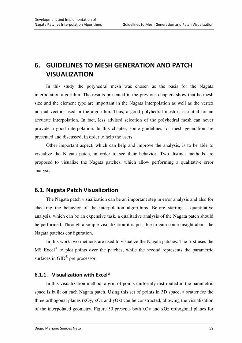
Development and Implementation of
Nagata Patches Interpolation Algorithms Guidelines to Mesh Generation and Patch Visualization
Diogo Mariano Simões Neto 59
6. GUIDELINES TO MESH GENERATION AND PATCH
VISUALIZATION
In this study the polyhedral mesh was chosen as the basis for the Nagata
interpolation algorithm. The results presented in the previous chapters show that he mesh
size and the element type are important in the Nagata interpolation as well as the vertex
normal vectors used in the algorithm. Thus, a good polyhedral mesh is essential for an
accurate interpolation. In fact, less advised selection of the polyhedral mesh can never
provide a good interpolation. In this chapter, some guidelines for mesh generation are
presented and discussed, in order to help the users.
Other important aspect, which can help and improve the analysis, is to be able to
visualize the Nagata patch, in order to see their behavior. Two distinct methods are
proposed to visualize the Nagata patches, which allow performing a qualitative error
analysis.
6.1. Nagata Patch Visualization
The Nagata patch visualization can be an important step in error analysis and also for
checking the behavior of the interpolation algorithms. Before starting a quantitative
analysis, which can be an expensive task, a qualitative analysis of the Nagata patch should
be performed. Through a simple visualization it is possible to gain some insight about the
Nagata patches configuration.
In this work two methods are used to visualize the Nagata patches. The first uses the
MS Excel®
to plot points over the patches, while the second represents the parametric
surfaces in GID®
pre processor.
6.1.1. Visualization with Excel®
In this visualization method, a grid of points uniformly distributed in the parametric
space is built on each Nagata patch. Using this set of points in 3D space, a scatter for the
three orthogonal planes (xOy, xOz and yOz) can be constructed, allowing the visualization
of the interpolated geometry. Figure 50 presents both xOy and xOz orthogonal planes for

Development and Implementation of
Guidelines to Mesh Generation and Patch Visualization Nagata Patches Interpolation Algorithms
60 Diogo Mariano Simões Neto
three geometries (cylinder, sphere and torus) as represented using Excel®
visualization
strategy. This methodology can be applied for both triangular and quadrilateral Nagata
patches, as shown in this figure. Note that the results shown in figure were obtained when
the normal vectors are provided by the analytical functions.
xOy plane xOz plane
Cy
lin
der
Sp
her
e
To
rus
Figure 50. Visualization of Nagata patches using MS Excel®.
6.1.2. Visualization with GID® Software
The second method uses GID®
pre processor to visualize the Nagata patches. As seen
previously in Chapter 2, concerning the Nagata patch formulation, both the triangular and
the quadrilateral patches are parametric surfaces. GID®
allows to create and represent
parametric surfaces using its mathematical formulas. The surface created is a NURBS that
approximates the real geometry. Figure 51 shows the same geometries presented in Figure
50, using GID®
to perform the Nagata patch visualization.
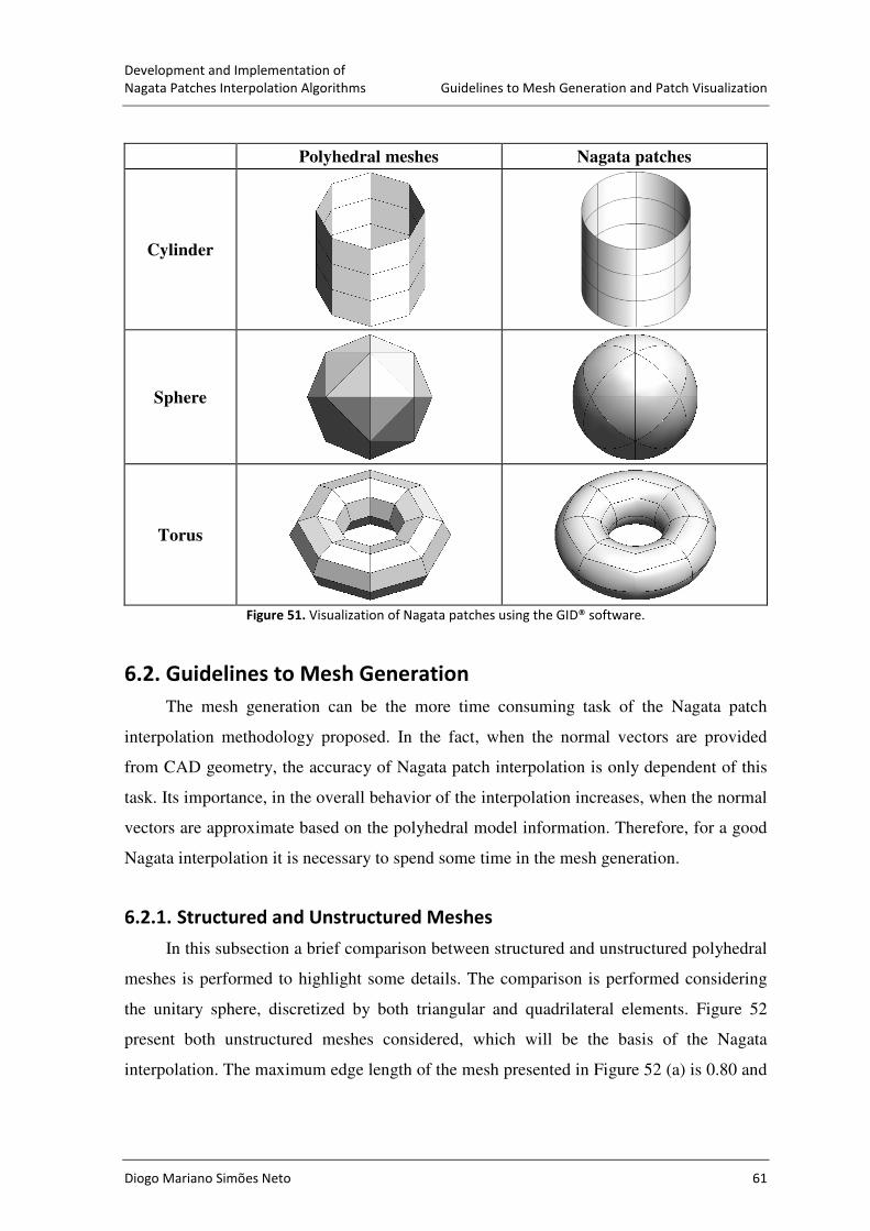
Development and Implementation of
Nagata Patches Interpolation Algorithms Guidelines to Mesh Generation and Patch Visualization
Diogo Mariano Simões Neto 61
Polyhedral meshes Nagata patches
Cylinder
Sphere
Torus
Figure 51. Visualization of Nagata patches using the GID® software.
6.2. Guidelines to Mesh Generation
The mesh generation can be the more time consuming task of the Nagata patch
interpolation methodology proposed. In the fact, when the normal vectors are provided
from CAD geometry, the accuracy of Nagata patch interpolation is only dependent of this
task. Its importance, in the overall behavior of the interpolation increases, when the normal
vectors are approximate based on the polyhedral model information. Therefore, for a good
Nagata interpolation it is necessary to spend some time in the mesh generation.
6.2.1. Structured and Unstructured Meshes
In this subsection a brief comparison between structured and unstructured polyhedral
meshes is performed to highlight some details. The comparison is performed considering
the unitary sphere, discretized by both triangular and quadrilateral elements. Figure 52
present both unstructured meshes considered, which will be the basis of the Nagata
interpolation. The maximum edge length of the mesh presented in Figure 52 (a) is 0.80 and

Development and Implementation of
Guidelines to Mesh Generation and Patch Visualization Nagata Patches Interpolation Algorithms
62 Diogo Mariano Simões Neto
of the mesh in Figure 52 (b) is 0.53. The normal vectors in each node of the polyhedral
meshes were determined using the analytical function.
(a) (b)
Figure 52. Unstructured mesh of a sphere composed by: (a) triangular elements; (b) quadrilateral elements.
Figure 53 present both radial and normal vector error distributions in the Nagata
patches interpolation for the polyhedral model presented in Figure 52 (a). It can be
observed that both maximum error values are localized near the edge with highest length,
as for structured meshes (see, for instance Figure 19 ). However, for unstructured meshes
the length edge dispersion is greater, leading to higher and more localized errors. Ideally,
the triangular elements should all have the same shape to produce an interpolation error
with a distribution as uniform as possible. The ideal form of the triangular element is to
have equal sides and angles.
The second model used, shown in Figure 52 (b), is composed by quadrilateral
elements. The error distributions in the quadrilateral Nagata patches interpolation are
shown in Figure 54. It can be observed that the patches present distinct radial error ranges,
due to the presence of distorted elements. To create a mesh interpolation with a uniform
error distribution, the quadrilateral elements must be rectangular or square, with all four
right angles.
[%] Radial error (δr) Normal vector error (δn) [º]
Figure 53. Radial and normal vector errors on the triangular patches used to describe the sphere.

Development and Implementation of
Nagata Patches Interpolation Algorithms Guidelines to Mesh Generation and Patch Visualization
Diogo Mariano Simões Neto 63
[%] Radial error (δr) Normal vector error (δn) [º]
Figure 54. Radial and normal vector errors on the quadrilateral patches used to describe the sphere.
6.2.1.1. Mesh Size
Besides the mesh typology and topology, the mesh size directly influences the
accuracy of the Nagata interpolation, as already highlighted in the previous chapters. These
previous results shows that more refined mesh result in lower error distributions for the
Nagata patch interpolations. However, those results also show that the element size must
be sensitive to the surface geometry. Thus, the element size must change in order to obtain
smaller error dispersion. Figure 55 presents an example using three different element sizes
to describe three arcs of circle with different radii. The use of different sizes leads to an
interpolation of all edges (6 elements) with the same error distribution, where the radial
error attains the maximum value (0.32%) in the middle of the edges (see Figure 8).
Figure 55. Elements with different sizes to describe a 2D geometry with curvature variation.
The nodes location dictates the Nagata patch position, which should be such that the
interpolation error is minimized. The central idea is to generate a higher density of nodes in
the zones with higher curvature change, in order to improve the surface description with
Nagata patches. If possible, all flat surfaces (zero mean curvature) must be discretized with

Development and Implementation of
Guidelines to Mesh Generation and Patch Visualization Nagata Patches Interpolation Algorithms
64 Diogo Mariano Simões Neto
only one element. This allows improving the error distribution and also reduces the total
number of elements needed to describe the geometry. When the surface has null curvature
in one direction, such as the cylinder, is recommended to use only one element in that
direction for the same reasons.
6.2.2. Geometry with Inflection Points
A single Nagata patch has no ability to describe a curve or surface with inflection
points due to its quadratic formulation. Therefore, ideally all inflection points should
correspond to a node, in order to define a boundary for the Nagata patches. The search for
inflection points on a surface is not an easy task, as well as the generation of a mesh with
nodes in all inflection points.
According with the study performed, there is an area near an inflection where the
nodes can be located without compromising too much the approximation error. The size of
this zone depends on the curvature value of the surface and the position of the nodes with
connectivity with it. If a node is located on this area, the inflection point of the geometry
described by the Nagata patches will be located on the node, which may have a different
location from the inflection point of the original geometry.
Figure 56. Localization for the node near of inflection point.
Figure 56 present an example of the admissible area for the node corresponding to
the inflection point. The admissible region for the node is divided in two sets, one on each
side of the inflection point, where the limits of each set is denoted by hollow symbols
(square and triangle). These limits are dependent on the position of the neighboring nodes,
denoted by solid symbols, and also by the curve curvature. When the node corresponding
to an inflection point is positioned in a limit of the admissible region, the result is a linear
interpolation between the opposite nodes, as shown in Figure 56 by the dashed lines. If the

Development and Implementation of
Nagata Patches Interpolation Algorithms Guidelines to Mesh Generation and Patch Visualization
Diogo Mariano Simões Neto 65
node corresponding to the inflection point is outside the region, the Nagata curve presents
a very sharp bend near the node, because the algorithm will always try to ensure the
boundary conditions.
To better understand the importance of inflection points in the Nagata interpolation
an example in which the nodes corresponding to the inflection points are poorly located is
shown. The aim is analyze a Nagata patch interpolation using a mesh that causes problems,
due to the points of inflection. The geometry chosen to make the interpolation is shown in
Figure 57 (a), where the inflection zone is visible. Figure 57 (b) presents the quadrilateral
mesh produced from NURBS surface, considering a uniform division into three elements
in one direction and five elements in the other direction.
(a) (b)
Figure 57. Geometry used to analyze the presence of inflection points: (a) NURBS surface; (b) quadrilateral
mesh.
The Nagata interpolation algorithm was applied to the polyhedral mesh using the
normal vectors provided by CAD geometry. Figure 58 (a) presents the interpolation
qualitative analysis, using the GID®
to visualize the Nagata patch, while Figure 58 (b) plots
the grid of points in the xOy plane. It can be observed, that the three patches in the centre
of the geometry have an irregular behavior, due to the fact that the nodes of the mesh
associated to inflection points are outside the admissible region. Thus, this leads to patches
with strange behavior, which can be observed and detected using both visualization
methods. In GID®
a dark zone in the patch identifies this behavior, while in Excel®
there is
a concentration of points.

Development and Implementation of
Guidelines to Mesh Generation and Patch Visualization Nagata Patches Interpolation Algorithms
66 Diogo Mariano Simões Neto
(a) (b)
Figure 58. Representation of the interpolation using: (a) GID® software; (b) the Excel® for the xOy plane.
Having identified the problem, it is necessary to develop a methodology to overcome
it, i.e. a method to indentify the inflection points. One possible method for determining the
inflection point is by calculating the surface curvatures, since the inflection point
corresponds to a point of discontinuity in the curvature (minor and major signed
curvature). However, the inflection point calculation through curvature is a difficult task to
perform numerically. Another way to identify these points on the NURBS surfaces is
through the position of control points. This method has not been well explored but seems
like a reasonable approach to solve the problem. Figure 59 presents an example of a
NURBS curve with an inflection point indicate by a hollow circle. This point can be
calculated determining the intersection of the straight line joining the two control points
and the NURBS curve, since by definition, the interpolated curve is always located in the
interior of the grid defined by the control points (see Figure 59). To validate this idea,
further testing for curves with various degrees and number of control points should be
performed.
Figure 59. Strategy to identify inflection points on a NURBS curve.
Development and Implementation of
Nagata Patches Interpolation Algorithms Guidelines to Mesh Generation and Patch Visualization
Diogo Mariano Simões Neto 67
6.3. Output Files Description
Output files are important to visualize, analyze and apply the Nagata patch
interpolations. In fact, once the Nagata patch interpolations are checked, it will be used as
input files to describe contact surfaces in FEA.
In the adopted strategy, three types of files are generated:
1 - File for analysis with MS Excel®
: This file is produced considering a grid of
points uniformly distributed over the Nagata patches. For each Nagata patch,
the number of grid point, its coordinates, normal vector components,
geometrical and normal vector error, are presented. Thus, these file allows
plotting points of the patches, as shown in Figure 50, or performing
quantitative analysis of error distributions, as shown, for instance, in Figure 20.
Appendix D shows an example of this file.
2 - File for analysis in GID®
post processor: In order to visualize the error
distributions over the Nagata patches, the information presented in previous
file can be combined with a very fine mesh built on the CAD surface, using the
same strategy already described in section 3.2. This strategy allows to produce
a file of results (*.res), which can be associated to the very fine polyhedral
model (*.msh). This allows the qualitative and quantitative analysis of the
results with GID®
post processor, as shown, for instance, in Figure 13.
3 - File for analysis in GID®
pre processor: This file contains the information
concerning the interpolation coefficients of equations (4) and (9). Thus, for
triangular Nagata patch six coefficients are presented, while for quadrilateral
patch eight coefficients are necessary. All these coefficients are vectors with
three components. Appendix D shows an example of this type of file, which
can be used as input for subsequent applications.

Development and Implementation of
Conclusions Nagata Patches Interpolation Algorithms
68 Diogo Mariano Simões Neto
7. CONCLUSIONS
The work presented had as starting point the algorithm for interpolating discretized
surfaces proposed by Nagata (2005). Both the triangular and quadrilateral Nagata patches
interpolation algorithms were implemented, in Fortran 90/95.
The first step of the work was the validation of the implemented algorithms using
simple geometries, with known normal vector, in each vertex. The validation was
performed considering one geometry in the 2D space (arc of a unitary circle) and four
geometries in the 3D space (plane, cylinder, sphere and torus). The error analysis
performed with the 2D geometry indicates that both the radial and the normal vector error
decrease with the decrease of the normalized edge length. Thus, the geometry converges to
the original geometry. The same occurs with the polyhedral model, which presents a
quadratic order of convergence for the radial error and linear for the normal vector error.
For the Nagata algorithm, the order of convergence of the radial error is quartic while it is
cubic for the normal vector error. These results highlight the enormous advantage of using
the Nagata interpolation, since it allows to recover the curve geometry and curvature with a
fewer number of elements. The error analysis performed with the 3D geometries indicates
that:
� In case of the cylindrical geometry, the maximum radial error is independent of the
number of elements in the axial direction and it is only dictated by the number of
elements in the circumferential direction. The order of convergence to the
analytical cylindrical surface is dictated only by the mesh description in the
circumferential direction and is the same of the arc of a circle, with quartic order of
convergence. These results are in agreement with the one presented in Nagata
(2005). For quadrilateral patches, also the normal vector error is independent of the
number of elements along the axial direction. However, for triangular Nagata
patches, the normal vector error decreases with the decrease of the number of
elements in the axial direction. Thus, triangular and quadrilateral Nagata patches
interpolations of polyhedral models, with the same normalized edge length along
the circumferential direction and only one element in the axial direction, will

Development and Implementation of
Nagata Patches Interpolation Algorithms Conclusions
Diogo Mariano Simões Neto 69
present the same radial error range. However, the distributions will be more
favorable for the triangular interpolations, since they always present more nodes
and, consequently, more information for the Nagata patch interpolation algorithm.
� In the case of the sphere it is shown that the interpolations performed with
triangular interpolations tend to describe a surface exterior to the sphere while
quadrilateral interpolations describe a more interior surface. The maximum positive
value of radial error and the maximum normal vector error always occurs in the
middle of the edge with highest length, regardless of its orientation, since the
sphere presents the same curvature in all points. When applying the two types of
Nagata interpolations to the same polyhedral model of the sphere, the radial error
average value is lower and the distribution is narrower for triangular interpolations
than for quadrilateral interpolations and also the normal vector error distributions
presents a lower average value for triangular interpolations. Thus, the error
distribution is more favorable for triangular Nagata patch interpolations.
� In the case of the torus, triangular and quadrilateral Nagata patch interpolations
lead to different error distributions. For triangular patches, both errors attain their
maximum values in the middle of the edges aligned with the major radius direction
of the torus. For quadrilateral patches the maximum (positive) radial error is
located at hyperbolic points and patches with negative error are located in the
region far from the axis of the torus, where the geometry is concave in all
directions. The normal vector error attains its maximum value in the region where
the radial error alters from positive to negative. Although the error distributions are
different, in order to reduce the maximum radial error it is necessary to increase the
number of elements in the major radius direction, for both triangular and
quadrilateral Nagata patches. It is observed that, although the triangular meshes
have two times more nodes than the quadrilateral meshes, the maximum error is
approximately the same. However, also for this geometry, both errors distributions
are more favorable for the triangular Nagata patch interpolation.
In brief, to improve Nagata patch interpolations it is necessary to decrease the
maximum edge length for non linear directions. These results are consistent with the ones
obtained with the 2D geometry, which can be used as guidelines for maximum edge
selection. The comparison between triangular and quadrilateral patches indicates that the

Development and Implementation of
Conclusions Nagata Patches Interpolation Algorithms
70 Diogo Mariano Simões Neto
first can lead to more favorable error distributions, even when applied to the same
quadrilateral model. This conclusion is also in agreement with the one presented in Nagata,
(2005).
The second step of the work involved the selection of algorithms for normal vector
approximation, for each vertex of the polyhedral model. Six different algorithms were
implemented and tested with the three simple geometries, cylinder, sphere and torus. Their
performance was compared taking into account the error in the normal error approximation
as well as the radial and normal vector error of the Nagata patches interpolation, generated
with the approximated normal vector. The analysis of the cylinder open surface shows that
all algorithms are sensitive to boundaries, which results in much larger normal vector
approximation errors for nodes located in these areas. The polyhedral models of the sphere,
considered in this analysis, are characterized by a larger number of nodes for the
quadrilateral. Thus, the results obtained indicate that the normal vector approximation error
is always higher for triangular models, except with the MWA algorithm. In fact, the
analysis of the MWA algorithm indicates that this method seems to be more suitable for
polyhedral descriptions with smaller angles (always less than 90º). The MWSELR
algorithm leads a zero error for both types of polyhedral descriptions, applied to the sphere.
These results obtained for the MWA algorithm are confirmed in the analysis of the torus
geometry. In this case, the maximum error in the normal vector approximation is always
higher for the triangular mesh. This is related to the fact that all edges of the quadrilateral
elements are oriented along the principal curvature directions. Unfortunately, the analysis
of the normal vector approximation errors is important but not sufficient to evaluate the
Nagata patches interpolation. In fact, the analysis of the sphere indicates that there is a
direct (non linear) relationship between the normal vector approximation error and the
radial error. However, in case of torus geometry the increase of the normal vector
approximation error does not necessarily result in an increase of the radial error range, on
the contrary it may even decrease. This results from the fact that the normal vector
approximation error introduces changes in the boundary conditions, which can lead to
different Nagata patch interpolation errors. Thus, although the MWSELR algorithm seems
to present the best behavior, the selection of the algorithm is always dependent of the
surface geometry and the polyhedral model adopted. For a complex geometry, for which
the normal vector is unknown, it is always possible to compare the normal vector

Development and Implementation of
Nagata Patches Interpolation Algorithms Conclusions
Diogo Mariano Simões Neto 71
approximation between the different algorithms, in order to help in the selection of the
algorithm.
Finally, the Nagata patches interpolation algorithm using normal vector determined
from CAD geometry was developed, implemented and validated using a real deep drawing
tool example. The results show that the normal vector estimative is accurate, which leads
to accurate interpolations in the entire domain of the polyhedral model, since the algorithm
is not sensitive to boundary elements. Thus, this algorithm allows bridging the gap
between CAD and CAE models, since it allows the interpolation of discretized surfaces
recovering the original CAD geometry.
Based on the results presented in this work and in Neto et al., (2010a) and Neto et
al., (2010b) some guidelines for polyhedral mesh generation, in order to guarantee accurate
Nagata patches interpolations, were detailed. In order to support the developments
presented in this work and further applications of Nagata patches interpolations, tools for
visualization and analysis (qualitative and quantitative) were developed and were also
presented. The combination of the implemented numerical tools with the GID®
pre
processor allows generating Nagata patches interpolations for any simple or complex
surface geometry.

Development and Implementation of
References Nagata Patches Interpolation Algorithms
72 Diogo Mariano Simões Neto
8. REFERENCES
Alves, J.L. (2003), “Simulação Numérica do Processo de Estampagem de Chapas
Metálicas - Modelação Mecânica e Métodos Numéricos”. PhD Thesis,
Department of Mechanical Engineering, University of Minho, Guimarães,
Portugal.
Baptista, A.J. (2006), “Modelação Mecânica e Simulação Numérica do Processo de
Estampagem Multi-Etapas - Aplicação ao Processo de Estampagem de Chapas
Soldadas”. PhD Thesis, Department of Mechanical Engineering, University of
Coimbra, Coimbra, Portugal.
Cox, M. (1972), “The numerical evaluation of B-splines”, Journal of the Institute of
Mathematics and its Applications, 10, 134-149.
deBoor, C. (1972), “On calculating with B-splines”, Journal of Approximation Theory,
6, 50-62.
Department of CTW (2010), “Mechanics of forming processes: Deep drawing”. Faculty
of Science and Technology of the University of Twente, accessed July 11, 2010,
in: http://www2.tm.ctw.utwente.nl/deepdrawing/.
Gouraud, H. (1971), “Continuous Shading of Curved Surfaces”, IEEE Transactions on
Computers, C-20(6), 623–629.
Hahmann, S. and Bonneau, G.-P. (2003), “Polynomial surfaces interpolating arbitrary
triangulations”, IEEE Transactions on Visualization and Computer Graphics, 9
(1), 99–109.
Hahmann, S., Bonneau, G.-P. and Taleb, R. (2000), “Smooth Irregular Mesh
Interpolation” In: Cohen, A., Rabut, C., Schumaker, L.L. (Eds.), Curve and
Surface Fitting: Saint-Malo 1999, Vanderbilt University Press, Nashville, pp.
237–246.
Iglesias A. (2001), “Industrial Formats”, Department of Applied Mathematics and
Computational Sciences, University of Cantabria.
Jin, S., Lewis, R.R. and West, D. (2005), “A Comparison of Algorithms for Vertex
Normal Computation”, The Visual Computer, 21, 71–82.
Loop, C. (1994), “A G1 triangular spline surface of arbitrary topological type”,
Computer Aided Geometric Design, 11, 303–330.
Mann, S., Loop, C., Lounsbery, M., Meyers, D., Painter, J., DeRose, T. and Sloan, K.
(1992), “A Survey of Parametric Scattered Data Fitting Using Triangular
Interpolants”, In: Hagen, H. (Ed.) Curve and Surface Design. SIAM,
Philadelphia, pp. 145–172.
Max, N. (1999), “Weights for Computing Vertex Normals from Facet Normals”, Journal
of Graphics Tools, 4(2), 1–6.

Development and Implementation of
Nagata Patches Interpolation Algorithms References
Diogo Mariano Simões Neto 73
Nagata, T. (2005), “Simple Local Interpolation of Surfaces Using Normal Vectors”,
Computer Aided Geometric Design, 22, 327-347.
Nagata, T. (in press), “Smooth Local Interpolation of Surfaces Using Normal Vectors”,
Journal of Applied Mathematics.
Neamtu, M. and Pfluger, P.R. (1994), “Degenerate Polynomial Patches of Degree 4 and
5 Used for Geometrically Smooth Interpolation in � 3”, Computer Aided
Geometric Design, 11, 451–474.
Neto, D.M., Oliveira, M.C., Alves, J.L. and Menezes, L.F. (2010a), “Local Interpolation
for Tools Surface Description”, 10th
International Conference on Numerical
Methods in Industrial Forming Processes, Pohang, Republic of Korea, June 13-
17, 2010.
Neto, D.M., Oliveira, M.C., Alves, J.L. and Menezes, L.F. (2010b), “Smoothing the
Polyhedral Mesh Surface with Nagata Interpolations”, accepted to be
presentation in the 3rd
International Conference in Mathematical Methods in
Engineering, Coimbra, Portugal, October 21-24, 2010.
Nilsson, B. (2009), “Finite Element Procedures for Virtual Tribology”. PhD Thesis,
Department of Mathematical Sciences, Chalmers University of Technology and
University of Gothenburg, Gothenburg, Sweden.
Numisheet’93 (1993), Proceedings of the 2nd
International Conference and Workshop on
“Numerical Simulation of 3-D Sheet metal Forming Processes – Verification of
Simulation with Experiments”, Eds. A. Makinouchi, E. Nakamachi, E. Oñate, R.
H. Wagoner, Isehara, Japan, August 31-September 2 .
Oliveira, M.C. (2005), “Algoritmos e Estratégias de Gestão do Problema de Contacto
com Atrito em Grandes Deformações. Aplicação à Estampagem de Chapas
Metálicas”. PhD Thesis, Department of Mechanical Engineering, University of
Coimbra, Coimbra, Portugal.
Piegl, L. (1991), “On NURBS: A Survey”, IEEE Computer Graphics & Applications,
11, 55-71.
Santos, A. (1993), “Tool Descriptions and Contact Strategies Used in Static Explicit
FEM Code ITAS3D for Simulation of 3-D Sheet Metal Forming Processes”. PhD
Thesis, University of Tokyo, Japan.
Santos, A. and Makinouchi, A. (1995), “Contact Strategies to Deal with Different Tool
Descriptions in Static Explicit FEM of 3-D Sheet-Metal Forming Simulation”,
Journal of Materials Processing Technology, 50, 277-291.
Skordos, A.A., Monroy Aceves, C. and Sutcliffe, M.P.F. (2005), “Drape Optimisation in
Woven Composite Manufacturing”, 5th
International Conference on Inverse
Problems in Engineering, Cambridge, UK, 11-15 July 2005.
Stadler, M., Holzapfel, G.A. e Korelc, J. (2003), “Cn continuous modelling of smooth
contact surfaces using NURBS and application to 2D problems”, International
Journal for Numerical Methods in Engineering, 57, 2177-2203.
Thürmer, G. and Wüthrich, C. (1998), “Computing Vertex Normals from Polygonal
Facets”, Journal of Graphics Tools, 3(1), 43–46.

Development and Implementation of
References Nagata Patches Interpolation Algorithms
74 Diogo Mariano Simões Neto
Tsai, M.-C., Cheng, C.-W. and Cheng, M.-Y. (2003), “A real-time NURBS surface
interpolator for precision three-axis CNC machining”, International Journal of
Machine Tools & Manufacturing, 43, 1217-1227.
Wang, C.C.L., Wang Y., Yuen M.M.F. (2004), “On increasing the developability of a
trimmed NURBS surface”, Engineering with Computers, 20, 54-64.

Development and Implementation of
Nagata Patches Interpolation Algorithms Appendix A – IGES Format File
Diogo Mariano Simões Neto 75
9. APPENDIX A – IGES FORMAT FILE
IGES (Initial Graphics Exchange Specification) was developed in the early 80s, as a
part of a project with the National Bureau of Standards [Iglesias, 2001].
Translator GID - IGES S0000001
1H,,1H;,3HGID,33H C:/CEMUC/FA/60s.igs,,,26,,,,,,0,,0,,0,,1, G0000001
0,,5HCIMNE,9,,; G0000002
128 1 1 D0000001
128 9 NURBSURF 1D0000002
128,7,1,3,1,0,0,1,0,0,0,0,0,0,0.2696129,0.50025292,0.69102833, 1P0000001
0.81038681,1,1,1,1,0,0,1,1,1,1,1,1,1,1,1,1,1,1,1,1,1,1,1,1, 1P0000002
-2.804053,-5.16892,0,-3.0315653,-4.0968669,0,-3.0830998, 1P0000003
-2.6158131,0,-2.450814,-0.24658376,0,-1.5993302,1.3546726,0, 1P0000004
-1.2423752,3.0707054,0,-1.1892867,3.9613801,0,-1.250001, 1P0000005
4.729729,0,-2.804053,-5.16892,10,-3.0315653,-4.0968669,10, 1P0000006
-3.0830998,-2.6158131,10,-2.450814,-0.24658376,10,-1.5993302, 1P0000007
1.3546726,10,-1.2423752,3.0707054,10,-1.1892867,3.9613801,10, 1P0000008
-1.250001,4.729729,10,0,1,0,1; 1P0000009
S0000001G0000002D0000002P0000009 T0000001

Development and Implementation of
Appendix B – Projection of a Point on a NURBS Surface Nagata Patches Interpolation Algorithms
76 Diogo Mariano Simões Neto
10. APPENDIX B – PROJECTION OF A POINT ON A NURBS
SURFACE
Consider a generic point P in the Euclidean space, which is orthogonally projected
on the surface ( , )u vS , in order to determine point P' (see Figure 60) [Baptista, 2006 and
Stadler et al., 2003].
Figure 60. Projection of a point on a NURBS surface.
The distance vector ( , )u vr , which connects the point P to an arbitrary point ( , )u vS
of the surface, is defined as:
( , ) ( , ) .u v u v= −r S P (32)
Thus, the position of point P' can be obtained by two orthogonality conditions,
through dot product ( , ) ( , )u u v u v⋅S r and ( , ) ( , )v u v u v⋅S r , such that:
( , ) ( , ) ( , ) 0( ) ( ) ,
( , ) ( , ) ( , ) 0
u
u v
v
f u v u v u v
g u v u v u v
= ⋅ =⊥ ∧ ⊥ ⇒ = ⋅ =
S rS r S r
S r (33)
where uS and
vS are the first order partial derivatives of the NURBS surface. Thus, the
problem reduces to determining the solutions of the system of nonlinear equation in the
( , )u v variables, presented in equation (33), which can be performed using, for example,
the Newton–Raphson method, which for the thi iteration can be presented as:
( )1
( ) ( 1) ( 1) ( 1),
i i i i−− − − = − X X J F X (34)

Development and Implementation of
Nagata Patches Interpolation Algorithms Appendix B – Projection of a Point on a NURBS Surface
Diogo Mariano Simões Neto 77
with:
( )( )
( )
( 1)( 1)
( 1) ( 1)
( 1)( 1),
ii
i i
ii
f u
vg
− −− −
−−
= =
XF X X
X (35)
and ( 1)i−J , the Jacobian of ( )F X calculated at ( 1)i−X , given by:
( 1)
( 1)2
( 1)
2.
i
i
u uu u v uvi
u v uv v vv
f f
u v
g g
u v
−
−
−
∂ ∂ + ⋅ ⋅ + ⋅ ∂ ∂ = = ∂ ∂ ⋅ + ⋅ + ⋅ ∂ ∂
S r S S S r SJ
S S r S S r S (36)
The partial derivatives of the NURBS surface ( , )u vS can be found in Appendix C. It
is know that the Newton-Raphson algorithm presents quadratic convergence order only in
the vicinity of the solution. In fact, a good initial value is important to guarantee
convergence. In the implemented algorithm, the distance between point P and a set of
points of the surface, equally spaced in the parametric domain is evaluated. The initial
solution (0) (0) (0)( , )u v=X is the value that yields the closest surface point to P .

Development and Implementation of
Appendix C – Derivatives of a NURBS Surface Nagata Patches Interpolation Algorithms
78 Diogo Mariano Simões Neto
11. APPENDIX C – DERIVATIVES OF A NURBS SURFACE
In this appendix, the necessary expressions to evaluate the first- and second-order
derivatives in a point ( , )u vP of a NURBS surface ( , )u vS (see Figure 61) are described.
The formulation presented is based in [Baptista, 2006; Tsai et al., 2003 and Wang et al.,
2004].
S(u,v)
u
v
P
Su
Sv
Figure 61. First order derivatives in a point of a NURBS surface.
For the u parametric direction, the first and second order partial derivatives are
given by:
,
,
0 0
( , )( , )( , ) ,
n mi j
u i j
i j
R u vu vu v
u u= =
∂∂ = = ∂ ∂ ∑ ∑
SS P (37)
22
,
,2 20 0
( , )( , )( , ) .
n mi j
uu i j
i j
R u vu vu v
u u= =
∂∂ = = ∂ ∂ ∑ ∑
SS P (38)
The derivates ( , )v u vS and ( , )vv u vS are analog to the u direction thus, there are
omitted. The derivate ( , )uv u vS is given by:
22
,
,
0 0
( , )( , )( , ) .
n mi j
uv i j
i j
R u vu vu v
v u v u= =
∂∂ = = ∂ ∂ ∂ ∂ ∑ ∑
SS P (39)
Assuming that ( , )A u v represent the numerator and ( , )B u v the denominator of the
, ( , )i p
R u v functions, such as:

Development and Implementation of
Nagata Patches Interpolation Algorithms Appendix C – Derivatives of a NURBS Surface
Diogo Mariano Simões Neto 79
, , ,( , ) ( ) ( ) ,
i p j q i jA u v N u N v w= (40)
, , ,
0 0
( , ) ( ) ( ) .n m
k p l q k l
k l
B u v N u N v w= =
=∑ ∑ (41)
One can obtain more compact expressions, applying the rules for functions
derivatives and after some simplification, one obtains:
2
( , ) ( , ) ( , )( , )( , ) ,
( , ) ( , )
u uu
A u v B u v A u vR u vR u v
u B u v B u v
∂= = −
∂ (42)
2
2 2
2
3
( , ) ( , ) ( , ) 2 ( , ) ( , )( , )( , )
( , ) ( , )
2 ( , ) ( , ),
( , )
uu uu u uuu
u
A u v A u v B u v B u v A u vR u vR u v
u B u v B u v
A u v B u v
B u v
+∂= = −
∂
+
(43)
2
2
3
( , ) ( , ) ( , ) ( , ) ( , )( , )( , )
( , ) ( , )
2 ( , ) ( , ) ( , ) ( , ) ( , ) ( , ),
( , )
uv v u v uuv
v u uv
A u v B u v A u v A u v B u vR u vR u v
v u B u v B u v
A u v B u v B u v A u v B u v B u v
B u v
+∂= = −
∂ ∂
−+
(44)
where,
(1)
, , ,
0 0(1)
, , ,
(2) (2)
, , , , , ,
0 0(1) (1)
, , ,
(1)
,
( , ) ( ) ( )
( , ) ( ) ( )
( , ) ( ) ( ) and ( , ) ( ) ( )
( , ) ( ) ( )
( , ) ( )
n m
u k p l q k l
k l
u i p j q i j n m
uu i p j q i j uu k p l q k l
k l
uv i p j q i j
uv k p
B u v N u N v w
A u v N u N v w
A u v N u N v w B u v N u N v w
A u v N u N v w
B u v N u
= =
= =
=
=
= =
=
=
∑ ∑
∑ ∑
(1)
, ,
0 0
.
( )n m
l q k l
k l
N v w= =
∑ ∑
(45)
In the above equations, ( )
, ( )k
i pN u denotes the thk order derivative of , ( )i p
N u . The
functions ( )
, ( )k
i pN u can be calculated by:
( 1) ( 1)
, 1 1, 1( )
,
1 1
( ) ( )( ) .
k k
i p i pk
i p
i p i i p i
N u N uN u p
u u u u
− −− + −
+ + + +
= − − −
(46)

Development and Implementation of
Appendix D – Output Files Nagata Patches Interpolation Algorithms
80 Diogo Mariano Simões Neto
12. APPENDIX D – OUTPUT FILES
� File with the coordinates and normal vectors of the grid points for each patch.
Patch Point Coord_x Coord_y Coord_z Normal_x Normal_y Normal_z
1 1 0.1442E+01 0.6899E+01 0.0000E+00 0.5998E+00 -0.8001E+00 -0.8856E-16
1 2 0.1192E+01 0.6699E+01 -0.9742E-08 0.6503E+00 -0.7596E+00 0.1625E-02
1 3 0.9440E+00 0.6473E+01 -0.1732E-07 0.6940E+00 -0.7200E+00 0.2896E-02
1 4 0.6976E+00 0.6222E+01 -0.2273E-07 0.7316E+00 -0.6817E+00 0.3828E-02
1 5 0.4528E+00 0.5946E+01 -0.2598E-07 0.7640E+00 -0.6452E+00 0.4430E-02
1 6 0.2096E+00 0.5644E+01 -0.2706E-07 0.7918E+00 -0.6108E+00 0.4704E-02
1 7 -0.3189E-01 0.5317E+01 -0.2598E-07 0.8157E+00 -0.5785E+00 0.4641E-02
1 8 -0.2718E+00 0.4965E+01 -0.2273E-07 0.8363E+00 -0.5483E+00 0.4214E-02
� File with the interpolation coefficients of equation (4) for each triangular patch, to use
in GID®
.
-TRIANGULAR NAGATA PATCHES-
c00 c10 c01 c11 c20 c02
Patch: 1
-0.100E+01 -0.117E-07 0.234E-07 -0.471E+00 0.293E+00 0.471E+00
-0.612E-16 -0.828E+00 0.828E+00 -0.357E+00 0.121E+00 0.236E+00
0.000E+00 0.250E-08 0.828E+00 0.114E+00 -0.250E-08 -0.236E+00
Patch: 2
-0.707E+00 0.471E+00 0.114E+00 -0.114E+00 0.236E+00 0.262E-08
-0.156E-08 -0.943E+00 0.943E+00 -0.357E+00 0.236E+00 0.121E+00
0.707E+00 0.471E+00 0.114E+00 0.471E+00 -0.471E+00 -0.293E+00
Patch: 3
-0.707E+00 -0.471E+00 0.943E+00 -0.471E+00 0.471E+00 0.236E+00
-0.156E-08 -0.943E+00 -0.279E-08 -0.471E+00 0.236E+00 0.471E+00
0.707E+00 -0.471E+00 0.943E+00 -0.367E-08 -0.236E+00 -0.236E+00
� File with the interpolation coefficients of equation (9) for each quadrilateral patch, to
use in GID®
.
-QUADRILATERAL NAGATA PATCHES-
c00 c10 c01 c11 c20 c02 c21 c12
Patch: 1
0.144E+01 -0.463E+00 -0.250E+01 0.252E+00 0.463E+00 0.814E-01 -0.252E+00 -0.722E-06
0.690E+01 -0.347E+00 -0.188E+01 -0.220E+00 -0.577E+00 -0.126E+01 0.472E+00 0.169E+00
0.000E+00 0.360E+01 -0.108E-06 -0.107E+01 -0.155E+00 0.108E-06 0.126E+00 -0.632E+00
Patch: 2
0.515E+01 0.416E+00 -0.431E+01 -0.880E+00 -0.416E+00 0.602E+00 0.880E+00 -0.151E-05
0.682E+01 -0.240E+00 0.248E+01 -0.430E+00 -0.675E+00 -0.241E+01 0.977E-01 0.322E+00
0.000E+00 0.359E+01 0.000E+00 0.122E+01 -0.181E+00 0.000E+00 0.262E-01 -0.120E+01
Patch: 3
0.856E+01 0.252E+00 0.184E+01 0.164E+00 -0.252E+00 -0.525E+01 -0.164E+00 -0.113E-04
0.474E+01 -0.114E+00 -0.833E+00 0.264E+00 -0.522E+00 0.291E+01 -0.153E+00 -0.390E+00
0.000E+00 0.251E+01 0.000E+00 -0.375E+00 -0.140E+00 0.000E+00 -0.409E-01 0.146E+01


![arXiv · arXiv:0910.5008v2 [math.AG] 25 Oct 2010 NAGATA COMPACTIFICATION FOR ALGEBRAIC SPACES BRIAN CONRAD, MAX LIEBLICH, AND MARTIN OLSSON Abstract. We prove the Nagata compactification](https://static.fdocuments.in/doc/165x107/60500a9bd30ea723bc25434f/arxiv-arxiv09105008v2-mathag-25-oct-2010-nagata-compactification-for-algebraic.jpg)