DEVELOPMENT AND ANALYSIS OF GRASSHOPPER-LIKE …etd.lib.metu.edu.tr/upload/12608733/index.pdf ·...
145
DEVELOPMENT AND ANALYSIS OF GRASSHOPPER-LIKE JUMPING MECHANISM IN BIOMIMETIC APPROACH A THESIS SUBMITTED TO THE GRADUATE SCHOOL OF NATURAL AND APPLIED SCIENCES OF MIDDLE EAST TECHNICAL UNIVERSITY BY AYLĐN KONEZ EROĞLU IN PARTIAL FULFILLMENT OF THE REQUIREMENTS FOR THE DEGREE OF MASTER OF SCIENCE IN MECHANICAL ENGINEERING SEPTEMBER 2007
Transcript of DEVELOPMENT AND ANALYSIS OF GRASSHOPPER-LIKE …etd.lib.metu.edu.tr/upload/12608733/index.pdf ·...

DEVELOPMENT AND ANALYSIS OF GRASSHOPPER-LIKE JUMPING MECHANISM IN BIOMIMETIC APPROACH
A THESIS SUBMITTED TO THE GRADUATE SCHOOL OF NATURAL AND APPLIED
SCIENCES OF
MIDDLE EAST TECHNICAL UNIVERSITY
BY
AYL ĐN KONEZ EROĞLU
IN PARTIAL FULFILLMENT OF THE REQUIREMENTS FOR
THE DEGREE OF MASTER OF SCIENCE IN
MECHANICAL ENGINEERING
SEPTEMBER 2007
DEVELOPMENT AND ANALYSIS OF GRASSHOPPER-LIKE JUMPING
MECHANISM IN BIOMIMETIC APPROACH
submitted by AYL ĐN KONEZ EROĞLU in partial fulfillment of the requirements for the degree of Master of Science in Mechanical Engineering, Middle East Technical University by, Prof. Dr. Canan ÖZGEN Dean, Graduate School of Natural and Applied Sciences Prof. Dr. S. Kemal ĐDER Head of Department, Mechanical Engineering
Prof. Dr. Metin Akkök Supervisor, Mechanical Engineering Dept., METU
Examining Committee Members: Prof. Dr. Suat Kadıoğlu Mechanical Engineering Dept., METU Prof. Dr. Metin Akkök Mechanical Engineering Dept., METU Prof. Dr Abdulkadir Erden Mechatronics Engineering Dept., Atılım University Assoc. Prof. Dr. Đlhan Konukseven Mechanical Engineering Dept., METU Prof. Dr. Müfit Gülgeç Mechanical Engineering Dept., Gazi University
Date: 05.09.2007

iii
I hereby declare that all information in this document has been obtained and presented in accordance with academic rules and ethical conduct. I also declare that, as required by these rules and conduct, I have fully cited and referenced all material and results that are not original to this work.
Name, Last Name:
Signature:

iv
ABSTRACT
DEVELOPMENT AND ANALYSIS OF GRASSHOPPER-LIKE JUMPING
MECHANISM IN BIOMIMETIC APPROACH
Konez Eroğlu, Aylin
M.S., Department of Mechanical Engineering
Supervisor: Prof. Dr. Metin Akkök
September 2007, 125 pages
Highly effective and power efficient biological mechanisms are common in nature.
The use of biological design principles in engineering domain requires adequate
training in both engineering and biological domains. This requires cooperation
between biologists and engineers that leads to a new discipline of biomimetic science
and engineering. Biomimetic is the abstraction of good design from nature. Because
of the fact that biomimetic design has an important place in mechatronic
applications, this study is directed towards biomimetic design of grasshopper-like
jumping mechanism.
A biomimetic design procedure is developed and steps of the procedure have
followed through all the study. A literature survey on jumping mechanisms of
grasshoppers and jumping robots and bio-robots are done and specifically apteral
types of grasshoppers are observed. After the inspections, 2D and 3D mathematical
models are developed representing the kinematics and dynamics of the hind leg
movements. Body-femur, femur-tibia and tibia-ground angles until take-off are
obtained from the mathematical leg models. The force analysis of the leg models
with artificial muscles and biological muscles are derived from the torque analysis. A

v
simulation program is used with a simple model for verification. The horizontal
displacement of jumping is compared with the data obtained from the simulation
program and equation of motion solutions with and without air resistance.
Actuators are the muscles of robots that lead robots to move and have an important
place in robotics. In this scope, artificial muscles are studied as a fourth step of
biomimetic design. A few ready-made artificial muscles were selected as an actuator
of the grasshopper-like jumping mechanism at the beginning of the study. Because of
their disadvantages, a new artificial muscle is designed and manufactured for mini
bio-robot applications. An artificial muscle is designed to be driven by an explosion
obtained due to the voltage applied in a piston and cylinder system filled with
dielectric fluid. A 3.78-mm diameter Teflon piston is fitted with a clearance into a
Teflon cylinder filled with a 25.7- mm fluid height and maximum 225 V is applied to
the electrodes by using an electrical discharge machine (EDM) circuit. The force on
the piston is measured by using a set-up of Kistler piezoelectric low level force
sensor. The data obtained from the sensor is captured by using an oscilloscope, a
charge meter, and a GPIB connecting card with software, Agilent. From the
experiments, the new artificial muscle force is about 300 mN giving a 38:1 force to
weight ratio and percentage elongation is expected to be higher than that of the
natural muscles and the other artificial muscles. From the force analysis of the leg
model, it is shown that the measured force is not enough alone for jumping of an
about 500 mgr body. An additional artificial muscle or a single muscle designed with
the same operating principle giving higher force to weight ratio is recommended as a
future study.
Keywords: biomimetic design, jumping mechanism, grasshoppers, artificial
muscles, bio-robots

vi
ÖZ
ÇEKĐRGE BENZERĐ SIÇRAMA MEKANĐZMASININ BĐYOBENZETĐM
YAKLA ŞIMLA GEL ĐŞTĐRĐLMESĐ VE ANAL ĐZĐ
Konez Eroğlu, Aylin
Yüksek Lisans, Makina Mühendisliği Bölümü
Tez Yöneticisi: Prof. Dr. Metin Akkök
Eylül 2007, 125 sayfa
Yüksek seviyede etkin ve güç kullanımında verimli biyolojik mekanizmalar doğada
yer almaktadır. Biyolojik tasarım prensiplerinin mühendislik alanında kullanabilmesi
biyoloji ve mühendislik alanlarında yetenek gerektirir. Biyologların ve mühendislerin
bu ortaklaşa çalışma gereksinimi yeni bir disiplin olan biyobenzetim bilim ve
mühendisliğinin gelişimine yol açmıştır. Biyobenzetim, doğada var olan iyi
tasarımların taklit edilmesidir. Biyobenzetim mekatronik uygulamalarda önemli bir
yere sahiptir, bu nedenle bu çalışma çekirge benzeri sıçrama mekanizmasının
biyobenzetim tasarımını yönetmektedir.
Biyobenzetimle tasarım yöntemi geliştirilmi ş ve bu yöntemin basamakları bütün
çalışma boyunca takip edilmiştir. Çekirge sıçrama mekanizmalarının, sıçramalı
robotların ve biyo-robotların kaynak araştırması yapılmış ve özellikle çekirgelerin
kanatsız türleri gözlemlenmiştir. Bu çalışmadan sonra, arka bacak kinematik ve
dinamik hareketlerini veren 2 boyutlu ve 3 boyutlu matematik modeller
geliştirilmi ştir. Sıçramaya kadar olan vücut-femur, femur-tibia ve tibia-yer açıları bu
modellerden elde edilmiştir. Suni kaslı ve biyolojik kaslı bacak modellerinin kuvvet
analizi tork analizinden çıkartılmıştır. Doğrulama için simülasyon programı basit bir

vii
model ile kullanılmıştır. Sıçramanın yatay mesafesi bu simülasyon programı ile hava
dirençli ve dirençsiz hareket denklemlerinin sonuçları ile karşılaştırılmıştır.
Robotikte önemli bir yere sahip olan eyleyiciler robotları hareket ettiren kaslardır. Bu
nedenle, suni kaslar biyobenzetimle tasarımın dördüncü basamağı olarak
çalışılmıştır. Bu çalışmanın başında, çekirgemsi sıçrama mekanizmasının eyleyicisi
olarak birkaç hazır suni kas seçilmiştir. Bu kasların dezavantajları nedeniyle mini
biyo-robot uygulamaları için yeni bir kas tasarlanmış ve üretilmiştir. Dielektrik sıvı
ile dolu piston-silindir sistemine uygulanan voltajdan kaynaklanan patlama ile
sürülen bir suni kas tasarlanmıştır. 3.78 mm çaplı bir teflon pistonun boşluklu
yerleştirildi ği plastik silindirdeki 25.7 mm sıvı yüksekliğine elektrotlara eletro-
erozyon makina (EDM) devresinden maksimum 225 V uygulanmıştır. Kistler
piezoelektrik düşük seviye kuvvet algılayıcısı ile pistondaki kuvvet ölçülmüştür.
Algılayıcıdan gelen veriler, bir osiloskop, bir yük büyütücüsü ve GPIB iletişim kartı
ile bir yazılım, Agilent, kullanılarak toplanmıştır. Deneylere göre, yeni suni kasın
kuvveti yaklaşık 300 mN, kuvvetin ağırlığa oranı 38:1 ve boydaki uzama yüzdesinin
biyolojik kaslara ve diğer suni kaslara göre daha yüksek olması beklenmektedir.
Bacak modelindeki kuvvet analizine göre bu kuvvetin yaklaşık 500 mgr’lık bir
gövdeyi sıçratmak için yeterli olmadığı görülmüştür. Daha sonra çalışılmak üzere
ilave suni kaslı ya da kuvvetin ağırlığa olan oranı daha yüksek olan tek kaslı bir
tasarım önerilmektedir.
Anahtar Kelimeler: Biyobenzetimle tasarım, sıçrama mekanizması, çekirgeler, suni
kaslar, biyo-robotlar

viii
To My Parents, My Dear Husband and M. Kemal ATATÜRK

ix
ACKNOWLEDGEMENTS
The author would like to express her appreciation and thankfulness to Prof. Dr.
Abdulkadir Erden for his encouragements, advice, guidance, and support that created
this study. The author wishes to express her thanks to Prof. Dr. Metin Akkök for his
supports and advice.
The author also wishes to thank Assoc. Prof. Dr. Atef Qasrawi, Assoc. Prof. Dr. Fuad
Aliew, Asst. Prof. Dr. Bülent Đrfanoğlu, and Instructor Kutluk Bilge Arıkan for their
suggestions and comments. Also the author would like to thank Emrah Demirci,
Alper Güner, Dilek Özgör and Gözde Eminoğlu for their support and friendship. The
author wants to thanks Tahsin Tecelli Öpöz for his great effort on my experimental
studies.
The author would like to thank Hacettepe University, Department of Biology for
their contributions to capturing a special genius of grasshoppers, Pholidoptera, an
apteral type in Ankara. Special thanks to Atılım University, Department of
Mechatronics Engineering for material and laboratory support. The technical
assistance of Mehmet Çakmak is gratefully acknowledged.
Authors acknowledge the State Planning Organization of Turkey (DPT) for their
funding via the research project entitled “Development and implementation of micro
machining (especially Micro-EDM) methods to produce (design and manufacture) of
mini/micro machines/robots”.
The author thanks to Mustafa Kemal Atatürk for his gift, Türkiye. We would be
nothing without him. Finally many thanks to my parents and my husband, Barış
Eroğlu, for their invaluable and endless support in all my life. This thesis is dedicated
to my all family.

x
TABLE OF CONTENTS
ABSTRACT........................................................................................................... iv
ÖZ .......................................................................................................................... vi
DEDICATION..................................................................................................... viii
ACKNOWLEDGEMENT ..................................................................................... ix
TABLE OF CONTENTS.........................................................................................x
LIST OF TABLES ............................................................................................... xiv
LIST OF FIGURES ...............................................................................................xv
CHAPTER
1. INTRODUCTION ..............................................................................................1
1.1 Biomimetics and Biomimetic Design ............................................................2
1.2 Scope of the Thesis ........................................................................................5
2. LITERATURE SURVEY ON THE ANATOMY OF GRASSHOPPER............6
2.1 Anatomy of Grasshopper Legs......................................................................6
2.1.1 Anatomy of Grasshopper Muscles ...................................................9
2.1.2 Working Mechanism of Hind Leg Joints.......................................11
2.2 Grasshopper Jumping Mechanism ..............................................................13
3. JUMPING AND/OR HOPPING MECHANISMS AND INSECT-LIKE
ROBOTS............................................................................................................17
3.1 Hopping Machine ........................................................................................17

xi
3.2 Monopod Hopping Robots ..........................................................................17
3.3 Omni-Pede (Serpentine Robot) ..................................................................18
3.4 A Small, Insect-Inspired Robot ...................................................................19
3.5 Biomimetic Hexapod Robot........................................................................20
3.6 Cricket Micro-Robot ...................................................................................21
3.7 Quadruped Jumping Robot..........................................................................23
3.8 Lobster Robot ..............................................................................................24
4. MODELING AND ANALYSIS OF GRASSHOPPER-LIKE JUMPING
MECHANISM ...................................................................................................25
4.1 3D Leg Model..............................................................................................25
4.1.1 Mathematical Model Description for 3D Leg Model ....................25
4.1.2 Kinematic Analysis for 3D Leg Model..........................................26
4.1.3 Kinematic and Dynamic Analyses According to Experimental
Data ................................................................................................29
4.2 2D Leg Model..............................................................................................31
4.2.1 Mathematical Model for 2D Leg Model ........................................31
4.2.2 Kinematic Analysis ........................................................................32
4.2.3 Dynamic Analysis ..........................................................................33
4.3 Results of the 2D and 3D Leg Model .........................................................35
4.4 Results of the Torques of the 2D Leg Model ..............................................38
4.5 Kinematic Analysis of the 3D Leg Model with MSC. Adams
Simulation ...................................................................................................39
5. ARTIFICIAL MUSCLES AND DEVELOPMENT OF A NEW
ARTIFICIAL MUSCLE ....................................................................................42
5.1 Literature Survey on Artificial Muscles......................................................42
5.1.1 Braided Pneumatic Actuators (BPA); McKibben Artificial
Muscles; Air Muscles.....................................................................45
5.1.2 Shape Memory Alloys (SMA) .......................................................48
5.1.3 Electroactive Ceramics (EAC).......................................................50

xii
5.1.4 Electromagnetic..............................................................................51
5.1.5 Piezoelectric ...................................................................................51
5.1.6 Electroactive Polymer Artificial Muscle (EAP or EPAM)............52
5.1.7 Antagonistically-Driven Linear Actuator (ANTLA) .....................60
5.1.8 Baughman and Colleagues’ Artificial Muscles..............................60
5.1.9 A Comparison of Artificial Muscles..............................................61
5.2 Studies on Artificial Muscles ......................................................................64
5.2.1 A New Artificial Muscle Design and Manufacture .......................67
5.2.2 Characteristics of Force Sensor Set-up Used in the New
Artificial Muscle ............................................................................72
6. PRELIMINARY DESIGN OF JUMPING MECHANISM OF
GRASSHOPPER-LIKE ROBOT ..................................................................... 79
6.1 Design of Jumping Mechanism of Grasshopper-like Robot Model............79
6.2 Discussion of the Artificial Muscle Force...................................................82
7. CONCLUSIONS AND FURTHER RECOMMENDATIONS ........................ 84
7.1 Discussion and Conclusions........................................................................84
7.2 Suggestions for Future Work ......................................................................86
REFERENCES...................................................................................................... 88
APPENDICES .......................................................................................................98
APPENDIX
A. ANALYTICAL SOLUTION OF BODY HEIGHT AND BODY-FEMUR
ANGLE ............................................................................................................99
A.1 Calculation of Body-Height ......................................................................99
A.1.1 Polynomial Solution....................................................................100
A.1.2 Lagrange Interpolating Polynomials Solution ............................101
A.1.3 Least Square Regression, Polynomial Regression Solution .......101

xiii
A.1.4 Result of the Body Height Analysis............................................103
A.2 Calculation of Femur-Tibia (Knee) Angle ..............................................104
A.2.1 Polynomial Solution....................................................................106
A.2.2 Lagrange Interpolating Polynomials Solution ............................106
A.2.3 Least Square Regression, Polynomial Regression Solution .......106
A.2.4 Result of the Femur-Tibia Angle Analysis .................................108
B. CALCULATION OF BODY-FEMUR ANGLE ............................................110
C. 2D LEG MODEL RESULTS..........................................................................112
D. CALCULATION OF MASSES AND VOLUMES OF FEMUR-TIBIA.......113
E. DYNAMIC MODEL OF THE GRASSHOPPER LEG ..................................115
F. TORQUE RESULTS OF 2D LEG MODEL...................................................123
G. ARTIFICIAL MUSCLES ...............................................................................124
xiv
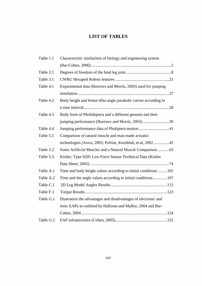
LIST OF TABLES
Table 1.1 Characteristic similarities of biology and engineering system
(Bar-Cohen, 2006) ..............................................................................2
Table 2.1 Degrees of freedom of the hind leg joint ............................................8
Table 3.1 CWRU Hexapod Robots features .....................................................21
Table 4.1 Experimental data (Burrows and Morris, 2003) used for jumping
simulation..........................................................................................27
Table 4.2 Body height and femur tibia angle parabolic curves according to
a time interval....................................................................................28
Table 4.3 Body form of Pholidoptera and a different genuise and their
jumping performance (Burrows and Morris, 2003) ..........................30
Table 4.4 Jumping performance data of Pholiptera motion..............................41
Table 5.1 Comparison of natural muscle and man-made actuator
technologies (Arora, 2005; Pelrine, Kornbluh, et.al, 2002 ...............45
Table 5.2 Some Artificial Muscles and a Natural Muscle Comparison............63
Table 5.3 Kistler, Type 9205 Low Force Sensor Technical Data (Kistler
Data Sheet, 2005) ..............................................................................74
Table A.1 Time and body height values according to initial conditions .........102
Table A.2 Time and the angle values according to initial conditions..............107
Table C.1 2D Leg Model Angles Results .......................................................112
Table F.1 Torque Results.................................................................................123
Table G.1 Illustration the advantages and disadvantages of electronic and
ionic EAPs as outlined by Halloran and Malley, 2004 and Bar-
Cohen, 2004 ....................................................................................124
Table G.2 EAP infrastructure (Cohen, 2005)...................................................125

xv
LIST OF FIGURES
Figure 1.1 The main topics of Biomimetic design procedure...............................3
Figure 1.2 Pictures of grasshoppers of Isophya Nervosa captured in Ankara ......4
Figure 2.1 Anatomy of a Grasshopper (Konez, Erden and Akkök, 2006)............7
Figure 2.2 Hind leg with segments identified (Fauske, 2002;
Laksanacharoen, Pollack, et al., 2005; Laksanacharoen, Quinn and
Ritzmann, 2003)...................................................................................7
Figure 2.3 Hinge Joint Model ...............................................................................8
Figure 2.4 Extensor muscle (top of the femur) and flexor muscle (bottom of
the femur) (Heitler, 2005) ...................................................................9
Figure 2.5 The structure of the lump a. the lump from the outside looks like
a pit, b. the lump sticks into the joint (Heitler, 2005) .........................9
Figure 2.6 Working strategy of the lump............................................................10
Figure 2.7 Muscles working mechanism (Heitler, 2005)....................................11
Figure 2.8 The joint region of a hind and middle legs a. hind leg knee joint,
b. middle leg knee joint (Heitler, 2005) ............................................12
Figure 2.9 Anatomy of the femur-tibia joint of a left hind leg of a mature
locust (Burrows and Morris, 2001) ...................................................12
Figure 2.10 The scanning electron micrograph of the a. spring cuticle (semi-
lunar process), b. normal cuticle (tibial cuticle, (Heitler, 2005))......13
Figure 2.11 The trajectory of a female Pholidoptera during a jump. The
numbers give the time before and after take-off at 0 ms (Burrows
and Morris, 2003)...............................................................................15
Figure 2.12 Selected frames from the same jump, a. Viewed from the side, b.
Viewed head-on (Burrows and Morris, 2003). .................................15
Figure 2.13 A routine program of grasshopper jumping (Heitler, 2005)..............16
Figure 3.1 a. 5 cm Monopod Hopping Robot, b. The simulated 2-D robot has
five degrees of freedom. Forces were modeled with springs and
dampers (Wei, Nelson, Quinn, Verma and Garverick, 2005)...............18

xvi
Figure 3.2 A view of OmniPede prototype (Granosik and Borenstein, 2004)......18
Figure 3.3 a. The jumping mechanism of Mini-Whegs in retracted (top) and
released (bottom) positions, b. Composite of video frames
showing Mini-Whegs jumping high over a 9 cm barrier
(Lambrecht, Horchler, et.al, 2005)....................................................19
Figure 3.4 a. An American Cockroach, b. Biobot (Delcomyn and Nelson,
2000) .................................................................................................20
Figure 3.5 Working process of the pneumatic muscle (Delcomyn and
Nelson, 2000) ....................................................................................20
Figure 3.6 Anatomy of the cricket micro-robot (Birch, Quinn, et al., 2005)......21
Figure 3.7 A view of the Cricket Cart Robot (Birch, Quinn, Hahm, Phillips,
et al., 2005)........................................................................................22
Figure 3.8 a. A Hybrid robot, b.One leg of the hybrid robot (Birch, Quinn,
et.al, 2005).........................................................................................22
Figure 3.9 Locomotion Concept of Jumping Quadruped (Kikuchi, Ota and
Hirose, 2003).....................................................................................23
Figure 3.10 A view of Quadruped Jumping Robot (Titech, 2006) ......................23
Figure 3.11 A view of Lobster robot (Safak and Adams, 2002)..........................24
Figure 4.1 The grasshopper (Pholidoptera) leg model (CM: Centre of Mass) ...26
Figure 4.2 The changes in the Femur-Tibia angle, body height and velocity
of body movement during a jump by a Pholidoptera male
(Burrows and Morris, 2003). ..............................................................27
Figure 4.3 a. Body height (z(t)), b. Femur-Tibia angle ( )(tα ) of body
movement of a Pholidoptera male before take-off for positive
time definite ......................................................................................28
Figure 4.4 2D Leg Model....................................................................................32
Figure 4.5 Position of a grasshopper leg until take-off.......................................33
Figure 4.6 Mass distribution of the leg model ....................................................33
Figure 4.7 Variations of Femur-Tibia, Body-Femur, and Ground-Tibia
angles until take-off...........................................................................36
xvii
Figure 4.8 Variations of position of centre of mass coordinates
until take-off.....................................................................................36
Figure 4.9 A plot of velocity until take-off ........................................................37
Figure 4.10 A body height variation along horizontal distance until take-off .....37
Figure 4.11 A graph of time-torque results of 2D leg model where T is the
total torque; T1 is the hip actuator torque; T2 is the knee actuator
torque.................................................................................................38
Figure 4.12 Total torque of 2D leg model ............................................................38
Figure 4.13 A grasshopper is modeled by using MSC. Adams Simulation
Program.............................................................................................39
Figure 4.14 Displacement analysis of grasshopper-Like by using MSC.
Adams 2005 ......................................................................................40
Figure 4.15 Like-grasshopper jumping analysis by using MSC. Adams 2005
R2 b. Velocity analysis, b. Kinetic energy analysis..........................40
Figure 5.1 A Swimming Robot Actuated by Living Muscle Tissue (Huge
Herr, Robert, 2004) ...........................................................................43
Figure 5.2 The force-length relationship of Braided Pneumatic Actuator’s
compared to that of muscle (Kingsley, 2005; Colbrunn, 2000)........46
Figure 5.3 A view of BPA a. A braided pneumatic actuator (Kingsley,
2005), b. An inflated (bottom) and uninflated (top) actuator
(Colbrunn, 2000) ...............................................................................46
Figure 5.4 Working Mechanism of a pneumatic muscle (Biorobotic, 2006)......47
Figure 5.5 Case Western University Hybrid Robot with rear leg, its actuator
is a McKibben Artificial muscle (Birch, et al., 2005).......................47
Figure 5.6 a. The hardware system of a leg design model, b. The leg model
(Colbrunn, 2000) ...............................................................................48
Figure 5.7 Basic Principles of SMA (Kapps, 2007)...........................................49
Figure 5.8 Polarization is a result of the alignment of piezoelectric domains
a. disk after polarization, b. applied voltage same polarity as
poling voltage: disk lengthens, c. applied voltage opposite

xviii
polarity as poling voltage: disk contracts (O’Halloran and
O’Malley, 2004)................................................................................51
Figure 5.9 A view of EAP, EPAM Roll Actuator from Artificial Muscle
(Lowe, 2006 ......................................................................................52
Figure 5.10 EAP actuators-energy density/frequency characteristics
(Ducheon, 2005)................................................................................52
Figure 5.11 Principle of operation EAP actuated devices (Bar-Cohen, 2000) .....53
Figure 5.12 A view of Ionic EAPs, a. Ionic gel at reference state, b. activated
state (O’Halloran and O’Malley, 2004; Bar-Cohen, 2004)...............54
Figure 5.13 a. An illustration of the IPMC gripper concept, b. A four-finger
gripper (Shahinpoor and Kim, 2004). ...............................................54
Figure 5.14 Electronic EAPs a. Ferroelectric polymer in the reference state
(left) and in its actuated state (right), b. circular strain test of a
dielectric elastomer with carbon grease electrodes c.
electrostrictive graft elastomer (O’Halloran and O’Malley, 2004)...55
Figure 5.15 Working mechanism of Dielectric EAP (Ashley, 2003) ...................56
Figure 5.16 Comparison of artificial muscle properties (Ashley, 2003) ..............57
Figure 5.17 A variety of actuator configurations for dielectric elastomers,
where the arrows the direction of actuation (O’Halloran and
O’Malley, 2004)................................................................................58
Figure 5.18 Spring Roll a. EAP roll actuator (Ducheon, 2005), b. Push-pull
actuators, c. Bending rolls (Ashley, 2003)........................................58
Figure 5.19 a. FLEX 2, b. Skitter (Pelrine, Kornbluh, Pei, Stanford, et.al,
2002) .................................................................................................59
Figure 5.20 An example of the Longitudinal EAP actuator
(Bar-Cohen, 1997).............................................................................59
Figure 5.21 Mechanical structure of ANTLA (Choi, Jung, Ryew, et.al, 2005)....60
Figure 5.22 Chronological order of invention of a few actuators/artificial
muscles..............................................................................................61
Figure 5.23 Max. Stress-Strain Graph for Actuator Materials (Bonser,
Harwin, Hayes, et.al, 2004)...............................................................62

xix
Figure 5.24 Actuator Max. Strain-Power Density Graph (Kapps, 2007)..............62
Figure 5.25 Pneumatic artificial muscle model (Festo, 2006) ..............................64
Figure 5.26 A view of set-up with Festo Pneumatic (McKibben) Artificial
Muscle (Atılım University, Biomimetic Design Laboratory) ...........65
Figure 5.27 A characteristic curve of Festo MAS 10 pneumatic muscles
(Festo, 2006) .....................................................................................66
Figure 5.28 Working mechanism of grasshopper-like leg set-up of Festo
pneumatic artificial muscle a. flexor artificial muscle is inflated,
b. extensor muscle is inflated............................................................66
Figure 5.29 A schematic view of the artificial muscle working mechanism........67
Figure 5.30 Piston and cylinder systems...............................................................68
Figure 5.31 A view of explosion due to electric discharge in piston-cylinder
artificial muscle (Atılım University, Machine Shop)........................69
Figure 5.32 A view of a vertical piston position set-up whose circuit is
detached from the EDM (Atılım University, Machine Shop)...........70
Figure 5.33 RC circuit set-ups a. with conventional micrometer and
insulation for electrical wire, b. with digital micrometer and
electrical isolation (Atılım University, Biomimetic Design
Laboratory)........................................................................................71
Figure 5.34 A plastic cylider- teflon piston system and its apparatus for using
EDM (Atılım University, Machine Shop).........................................71
Figure 5.35 The general construction of a. Kistler 9205 type force sensor, b.
coupling element where SW 5.5 is a fork wrench (Kistler data
sheet, 2005) .......................................................................................73
Figure 5.36 A view of Kistler force sensor set-up (Atılım University,
Machine Shop) ..................................................................................73
Figure 5.37 The artificial muscle mechanism.......................................................75
Figure 5.38 The artificial muscle mechanism with a coupling element and a
force sensor, Catia P3V5R10 ............................................................76
Figure 5.39 The construct of artificial muscle mechanism, coupling element
and force sensor and the force analysis set-up ..................................76

xx
Figure 5.40 A top view of the artificial muscle and the force sensor technical
drawing with dimensions, Catia P3V5R10 .......................................77
Figure 5.41 An output screen showing force sensor and applied voltage using
Agilent software for the experiments................................................77
Figure 6.1 A view of grasshopper-like bio-robot, Catia P3V5R10 drawing ......80
Figure 6.2 a. A protoype of design of leg model, Catia P3V5R10, b. The
working mechanism of new artificial muscle prototype in a
jumping leg model (Atılım University, Biomimetic Design
Laboratory)........................................................................................81
Figure 6.3 Position of centre of mass prototype in a jumping leg model until
take-off (Atılım University, Biomimetic Design Laboratory) ..........81
Figure 6.4 A view of leg model with extensor and flexor biological muscles....82
Figure 6.5 A view of leg model using single artificial muscle ...........................83
Figure A.1 Body height (z(t)) of body movement of a Pholidoptera male
before take-off for positive time definite ..........................................99
Figure A.2 Mathcad 2000 body height solutions, polynomial, Lagrange and
least square methods solutions........................................................104
Figure A.3 Femur-Tibia angle (α(t)) of body movement of a Pholidoptera
male before take-off for positive time definite ...............................105
Figure A.4 Mathcad 2000 femur-tibia angle solutions, polynomial, Lagrange
and least square methods solutions .................................................109
Figure D.1 Mathematical models of the femur and tibia ...................................113

1
CHAPTER 1
INTRODUCTION
Nature has highly effective and power efficient mechanisms. One of the recent
challenges in Mechatronics Engineering is to mimic biological systems in robot
design in engineering domain to make use of the efficient mechanisms in biological
domain. This approach is known as biomimetic design and may have significant
improvements in future engineering technology. The main aim of this work is to
develop a typical case study for biomimetic design. “Grasshopper jumping” is
selected as the topic of the case study. There is no particular reasoning in this
selection.
Legged locomotion has been used by biological systems since the beginning of the
biological life on earth. Although wheeled vehicles are so familiar and ubiquitous in
our modern way of life, legged vehicles, especially jumping locomotion, are
preference because of their better mobility in rough terrain (Savant, 2003) but they
need extra effort to control their locomotion (Delcomyn and Nelson, 2000). Actually,
surfaces for transportation like roadways and railways are not needed for the bio-
robot transportation.
Insects in particular are well known not only for their speed and agility but also for
their ability to traverse some of the most difficult terrains. Insects can be found
navigating sparse or rocky ground, climbing vertical surfaces, or even walking
upside down (Kingsley, 2005). In addition to walking, many insects jump to escape
from predators, to increase their speed across land, or to launch into flight. Some
insects, like bush crickets or grasshoppers, have long hind (rear) legs, so they can
leap longer distances than insects of comparable mass with shorter legs (Lambrecht,
Horchler and Quinn, 2005). Because of the challenge of these mechanisms jumping

2
mechanisms of the ensifera insects (e.g. crickets or grasshoppers) have been studied
as a good source for bio-robotics by many researchers. A grasshopper-like jumping
mechanism design is selected for biomimetic design in this thesis.
1.1 BIOMIMETICS AND BIOMIMETIC DESIGN
“The term biomimetics, which was coined by Otto H. Schmitt, represents the studies
and imitation of nature’s methods, mechanisms and processes”, Bar-Cohen, 2006.
Biomimetics (Biologically Inspired Technologies) is the abstraction of good design
from nature (University of Reading, 1992) and its aim is to mimic biological life or
systems (Leeuwen and Vreeken, 2004).
Biomimetic robots borrow their structure, senses and behavior from animals, such as
humans or insects, (Stanford, 2005) and plants. Biomimetic design is design of a
machine, a robot or a system in engineering domain that mimics operational and/or
behavioral model of a biological system in nature. One can take biologically
identified characteristics and seek an analogy in terms of engineering as shown in the
Table 1.1.
Table 1.1 Characteristic similarities of biology and engineering system (Bar-Cohen, 2006)
Biology Engineering BIO- engineering/ mimetics/ nics/ mechanics
Body System System with multifunctional materials and structures are developed emulating the capability of biological systems.
Skeleton and bones Structure and support struts
Support structures are part of every man-made system
Brain Computer Advances in computers are being made emulating the operation of the human brain
Intelligence Artificial intelligence
There are numerous aspects of artificial intelligence that have been inspired by biology including augmented reality, autonomous systems, computational intelligence, expert systems, fuzzy logic, etc
Senses Sensors Computer vision, artificial vision, radar, and other proximity detectors all have direct biological analogies.
Muscles Actuators Artificial muscles Electrochemical power generation
Rechargeable batteries
The use of biological materials to produce power will offer mechanical systems enormous advantages.

3
In this thesis the procedure given in Figure 1.1 is followed. The titles include a few
subtitles but they cannot be described clearly step by step. All of them are
mentioned in the related parts.
Biomimetic Design
Understanding Anatomy NO of Animal Basic Principles
of Biology YES
Understanding NO Robotic Studies in Biomimetic YES
Completing Mathematical NO Model Principles of Dynamic YES Mechanisms
NO Actuator Design
YES
Preliminary Design
Figure 1.1 The main topics of Biomimetic design procedure

4
Before starting any biomimetic design, an extensive survey and analysis of jumping
mechanism of the grasshopper in biology domain is necessary. There are many
geniuses of grasshoppers in and around the Ankara region. Apteral types are selected
to observe their behavior of the jumping locomotion. The species of the Isophya
nervosa are seen frequently in this region. Many of these are observed in their natural
environment and many others are captured and their bodies are studied (e.g. bodies’
weight, length of their real legs). A picture of the captured grasshoppers is given in
the Figure 1.2. Some useful data are collected, sorted, and analyzed for Isophya
nervosa. However, mechanical structure of the insect-like robot is modeled from the
Pholidoptera. This insect is selected as a model because its structure and physiology
are reasonably well known. A mathematical model is developed for the genius of
Pholidoptera. The data from the experimental results of the Pholidoptera is used to
evaluate the mathematical model. A new artificial muscle is developed to be used in
the mechanism.
Figure 1.2 Pictures of grasshoppers of Isophya Nervosa captured in Ankara
5
1.2 SCOPE OF THE THESIS
This work is intended to develop a jumping mechanism for a “grasshopper-like”
robot. Biomimetic design of an animal for robot technology can be classified by lots
of titles and subtitles. Organization of this thesis can be summarized according to this
classification. In Chapter 2, literature survey about grasshoppers is presented.
Anatomy of grasshoppers jumping mechanism, a biological force system of
grasshoppers, and jumping strategy of them are summarized in this chapter.
Jumping and hopping robots are discussed in Chapter 3. Biomimetic studies on robot
technology are examined briefly in this part. In Chapter 4, a mathematical model is
developed and its analysis is completed for the jumping mechanism. 2 DOF and 3
DOF models are studied and the position of a grasshopper’s hind legs is determined
from these models. Moreover, joints torque is analyzed.
In addition to these chapters, in Chapter 5, artificial muscles are considered as
actuators of biomimetic design. The technical features of some important artificial
muscles are tabulated. A challenge point of this thesis is the artificial muscle study.
An artificial muscle is not only developed but also added in the literature as a new
technological actuator. Force analysis of the actuator is completed with Kistler, Low
Level Force Piezoelectric Sensor. After design of the actuator, preliminary design of
grasshopper-like jumping mechanism is mentioned briefly in Chapter 6. All of
chapters are concluded and further recommendations are given in Chapter 7.

6
CHAPTER 2
LITERATURE SURVEY ON THE ANATOMY OF
GRASSHOPPER
As mentioned in the previous chapter, Biomimetic term comes from mimicking
nature. If nature systems are to be mimicked in engineering, anatomy of them should
be studied as a first step of biomimetic design. In this study, not only walking
mechanism of grasshoppers jumping system is presented but also two jumping styles
of grasshoppers are summarized briefly.
2.1 ANATOMY OF GRASSHOPPER LEGS
Grasshoppers have six legs, like most of the other insects, match in pairs across their
thorax. Anatomy of a grasshopper is illustrated in Figure 2.1 which was generated by
Enchanted Learning (1999) and Konez, Erden and Akkök (2006) to show the details
of the legs on the body. Figure 2.2 shows all of the six legs inherited from the same
animal- a locust of the species Schistocerca gregaria. Bigger rear (hind or
metathoracic, (Fauske, 2002)) leg is advantageous for jumping (Pfadt, 2002), because
it increases the length over which the jumper can exert a pushing force on the
ground.
Each of three pairs of legs, though very different in size and function, has five
distinct segments; coxa, trochanter, femur, tibia and tarsus as shown in Figure 2.2.
These segmental constructions are highly efficient for actuation, so grasshoppers
optimize their specialized locomotors’ behaviors (Birch, Quinn, et al., 2005). The
hind tibia has two rows of spines and enlarged movable spurs (calcaria or calcar,
(Fauske, 2002)) at its apex. The number of spines and the length of calcars vary

7
among species. There are two claws at the end of the tarsus, which give the
grasshopper a good gripping ability and prevent sliding when it pushes on the ground
as it jumps (Heitler, 2005). A pad between these claws is called arolium (Pfadt,
2002) and it has an important function to create friction with the ground surface.
Figure 2.1 Anatomy of a Grasshopper (Konez, Erden and Akkök, 2006)
Figure 2.2 Hind leg with segments identified (Fauske, 2002; Laksanacharoen,
Pollack, et al., 2005; Laksanacharoen, Quinn and Ritzmann, 2003).

8
Segment joints can have a single or multiple degrees of freedom (DOF) for a hind
leg. Those are given in Table 2.1. The significant feature of the coxa is the existence of
a soft tissue, 3 DOF joint that connects it to the body of the animal, enabling complex
positioning of the entire leg. Since the coxa segment is very small in all legs of the
grasshopper, it is ignored in robotics.
The trochanter is an even smaller segment, connecting the coxa and femur through two 1
DOF joints (Laksanacharoen, Pollack, et.al, 2005). The joint between the trochanter
and femur has very little movement; trochanter is considered to be negligible in the
biomimetic robot design approach, so reducing high level DOF is secured. Insect
legs also have a foot-like tarsus, but in order to keep the legs relatively simple, it is
modeled as a flexible plate. The femur-tibia (FT) and tibia-tarsus (TT) joints are also
1 DOF. With the exception of the mostly immobile trochanter-femur joint, all of the 1
DOF joints (a simple hinge joint, Figure 2.3) act in the same plane (Laksanacharoen,
Pollack, et.al, 2005).
Table.2.1 Degrees of freedom of the hind leg joint
Joint Degrees of Freedom (DOF)
Total DOF
Body-Coxa 3 DOF
Coxa-Femur 1 DOF
Coxa-Trochanter 1 DOF
Trochanter-Femur Very small movement
Coxa-Trochanter-Femur (CTF) joint is 1DOF
Body-Femur joint is 3DOF
Femur-Tibia (FT) 1 DOF
Tibia-Tarsus (TT) 1 DOF
Figure 2.3 Hinge Joint Model

9
2.1.1 Anatomy of Grasshopper Muscles
The hind femur is the enlarged jumping spring of the hind legs; it includes flexor and
extensor muscles inside the exoskeleton (hard shell). These muscles can be seen in
Figure 2.4. Because of its size and pennate anatomy, the extensor muscle is stronger
than the flexor. In a pennate muscle, the fascicles form a common angle with the
tendon. Because the muscle cells pull at an angle, contracting pennate muscles do not
move their tendons.
Figure 2.4 Extensor muscle (top of the femur) and flexor muscle (bottom of the
femur) (Heitler, 2005)
Although the flexor muscle’s size is smaller than extensor muscle’s, it can work as
nearly stronger as extensor muscle due to lump structure. In the knee of the hind leg
there is a structure which looks like a small black pit. This pit is in fact a lump that
sticks into the cavity of the femur (Figure 2.5).
a. b.
Figure 2.5 The structure of the lump a. the lump from the outside looks like a pit, b. the lump sticks into the joint (Heitler, 2005)

10
“The lump is absolutely crucial for the jump, because it enables the weak flexor
muscle to hold the tibia flexed against the strong extensor muscle during the energy
build-up”, Heitler, 2005. Working mechanism’s animation is given Figure 2.6. Two
features account for this:
• The lever system
The lump changes the angle with which the flexor tendon pulls on the tibia.
When the tibia is fully flexed, the flexor muscle has a very direct line of pull
on the tibia, while the extensor has a very indirect line of pull. The flexor thus
has a large mechanical advantage over the extensor muscle.
• The tendon pocket
An additional feature comes into play in the fully flexed position. There is a
small pocket in the middle of the flexor tendon, close to where it joins onto
the tibia. As the tibia comes into the fully flexed position, this pocket arrives
over the lump, and slides down onto it. This further increase the ability of the
flexor muscle to hold the tibia flexed against the strong extensor muscle.
Figure 2.6 Working strategy of the lump

11
2.1.2 Working Mechanism of Hind Leg Joints
Muscles working mechanism is given in Figure 2.7. When one of the muscle
contracts, it pulls on its tendon and moves the tibia one way, when the other muscle
contracts, it moves the tibia the other way (Heitler, 2005).
Figure 2.7 Muscles working mechanism (Heitler, 2005)
Grasshoppers have a like-catapult (semi-lunar process), the black half-moon shaped
region, in the hind legs made from special cuticle (Figure 2.4). This process is only
found on the hind legs–it is completely missing from the front and middle legs
(Figure 2.8). This structure has a similar function of a torsion spring and store energy
(Burrows and Morris, 2002; Heitler, 2005). About half of the jumping energy is
stored in these processes (Bennet-Clark, 1975; Burrows and Morris, 2002; Heitler,
2005) at femur-tibia joint (Figure 2.9) while the remainder is stored in extensor
tendon and cuticle of the femur (Bennet and Clark, 1975).

12
a. b.
Figure 2.8 The joint region of a hind and middle legs a. hind leg knee joint, b. middle leg knee joint (Heitler, 2005)
Figure 2.9 Anatomy of the femur-tibia joint of a left hind leg of a mature locust
(Burrows and Morris, 2001)
13
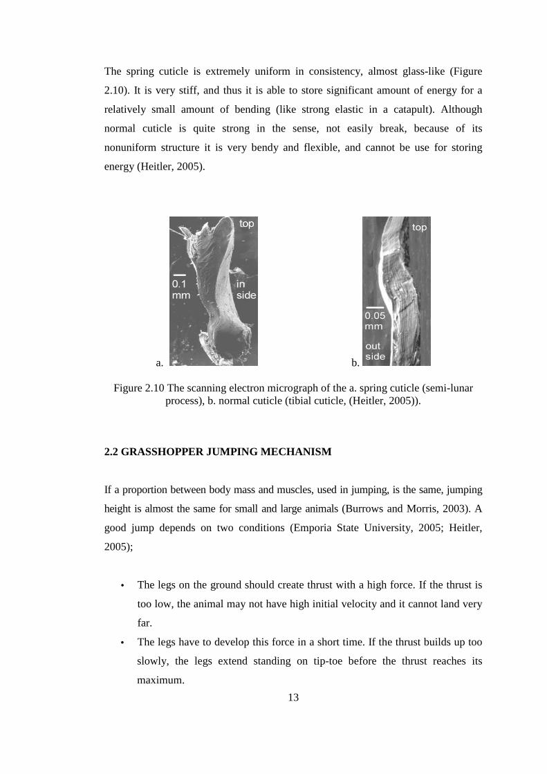
The spring cuticle is extremely uniform in consistency, almost glass-like (Figure
2.10). It is very stiff, and thus it is able to store significant amount of energy for a
relatively small amount of bending (like strong elastic in a catapult). Although
normal cuticle is quite strong in the sense, not easily break, because of its
nonuniform structure it is very bendy and flexible, and cannot be use for storing
energy (Heitler, 2005).
a. b.
Figure 2.10 The scanning electron micrograph of the a. spring cuticle (semi-lunar process), b. normal cuticle (tibial cuticle, (Heitler, 2005)).
2.2 GRASSHOPPER JUMPING MECHANISM
If a proportion between body mass and muscles, used in jumping, is the same, jumping
height is almost the same for small and large animals (Burrows and Morris, 2003). A
good jump depends on two conditions (Emporia State University, 2005; Heitler,
2005);
• The legs on the ground should create thrust with a high force. If the thrust is
too low, the animal may not have high initial velocity and it cannot land very
far.
• The legs have to develop this force in a short time. If the thrust builds up too
slowly, the legs extend standing on tip-toe before the thrust reaches its
maximum.
14
Two different jumping styles are proposed;
I. According to Burrows and Morris (2003), similar as Pholidoptera’s jumping
(Figure 2.11 and 2.12);
1. A jump begins with a forward rotation of the hind legs at their body-coxa
joints and a flexion of the tibia about the femur as shown in Figure 2.11. The
flexion of the tibia is not always complete so that one or both hind legs could
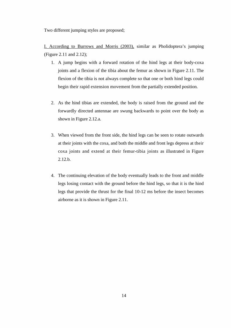
begin their rapid extension movement from the partially extended position.
2. As the hind tibias are extended, the body is raised from the ground and the
forwardly directed antennae are swung backwards to point over the body as
shown in Figure 2.12.a.
3. When viewed from the front side, the hind legs can be seen to rotate outwards
at their joints with the coxa, and both the middle and front legs depress at their
coxa joints and extend at their femur-tibia joints as illustrated in Figure
2.12.b.
4. The continuing elevation of the body eventually leads to the front and middle
legs losing contact with the ground before the hind legs, so that it is the hind
legs that provide the thrust for the final 10-12 ms before the insect becomes
airborne as it is shown in Figure 2.11.

15
Figure 2.11 The trajectory of a female Pholidoptera during a jump. The numbers give
the time before and after take-off at 0 ms (Burrows and Morris, 2003).
a. b.
Figure 2.12 Selected frames from the same jump a. Viewed from the side, b. Viewed head-on (Burrows and Morris, 2003).
II. According to Heitler (2005), grasshopper jumping goes through a set of routine
activity (a motor program) before it actually takes off as shown in Figure 2.7 and
2.13. The main difference between these two jumping styles is that Heitler’s motor
program has a co-activation in which flexor and extensor muscles contract together
which is fit with Hill’s muscle model. The contraction of the flexor muscle keeps the
tibia in the fully flexed position, so that the simultaneous contraction of the extensor

16
muscle bends the springs in the joint, rather than extending the leg. The extensor
muscle contraction is quite slow (about half a second), and this means that the
muscle can contract with maximum force. The energy of the contraction is stored in
the semi-lunar shaped region. The other difference is that knee (femur-tibia joint) is
closer to the surface when starting to the jumping instead of maintaining the initial
position, i.e. knee is movable.
Figure 2.13 A routine program of grasshopper jumping (Heitler, 2005)
In this chapter the anatomy of grasshoppers’ hind leg is summarized and compared
with mid and front legs. Extensor and flexor muscles and semi-lunar process of
grasshoppers are described briefly and working mechanism of legs and muscles’
significance are emphasized. Since the Pholidoptera structure and physiology are
reasonably well-known, and empirical data of this type are observed in the literature,
the studies of Burrows and Morris (2003) will be considered in proceeding chapters.
17
CHAPTER 3
JUMPING AND/OR HOPPING MECHANISMS AND INSECT-
LIKE ROBOTS
After the survey on the grasshoppers jumping mechanism in the literature, some
hopping and jumping machines and robots that utilizes of jumping mechanisms are
investigated as a second step of the biomimetic design.
3.1 HOPPING MACHINE
In 1983, a hopping machine, with only one leg, was built by Raibert at Carnegie-
Mellon University (Wei, Nelson, et al., 2005). The leg has three degrees of freedom.
The vertical motion was provided by a pneumatic cylinder, which is mounted on the
body frame via a gimbal joint.
3.2 MONOPOD HOPPING ROBOTS
Raibert (1986; 1993) developed several monopod robots that hop. Although they
were not statically stable, their controllers achieved active dynamic stabilization. He
showed that the control theory that governs the performance of monopod robots could
be used to control multi-legged ones. In contrast, Ringrose (1997) developed several
monopod robots that are not only statically stable, but are also passively dynamically
stable. The special shape of its foot creates this stability. The foot's curvature
causes a restoring torque to be imparted to the robot if it begins to tip over. Kingsley
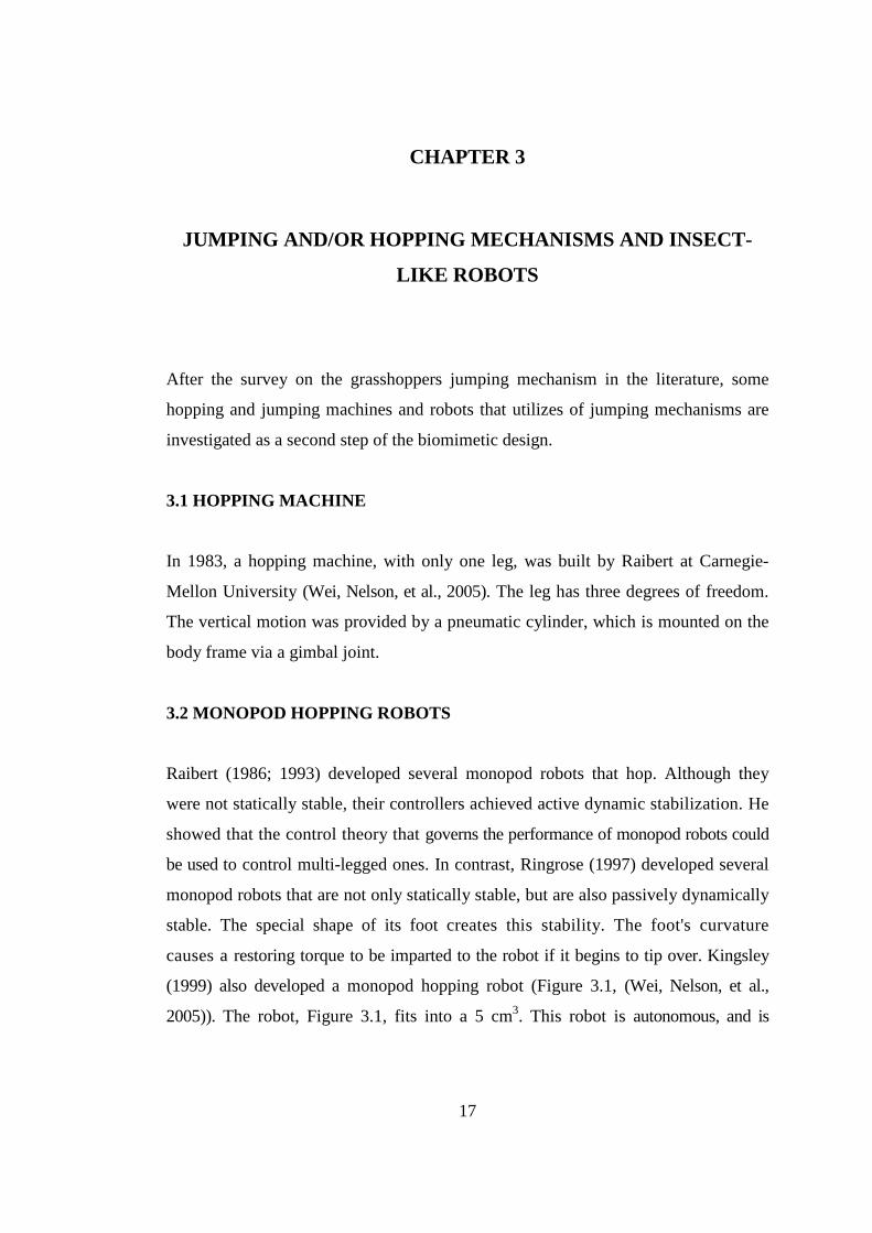
(1999) also developed a monopod hopping robot (Figure 3.1, (Wei, Nelson, et al.,
2005)). The robot, Figure 3.1, fits into a 5 cm3. This robot is autonomous, and is
18
designed to be statically and passively dynamically stable. Hopping is achieved through
the excitation of a spring-mass system at its resonant frequency.
a. b.
Figure 3.1 a. 5 cm Monopod Hopping Robot, b. The simulated 2-D robot has five degrees of freedom. Forces were modeled with springs and dampers (Wei, Nelson,
Quinn, Verma and Garverick, 2005).
3.3 OMNIPEDE (SERPENTINE ROBOT)
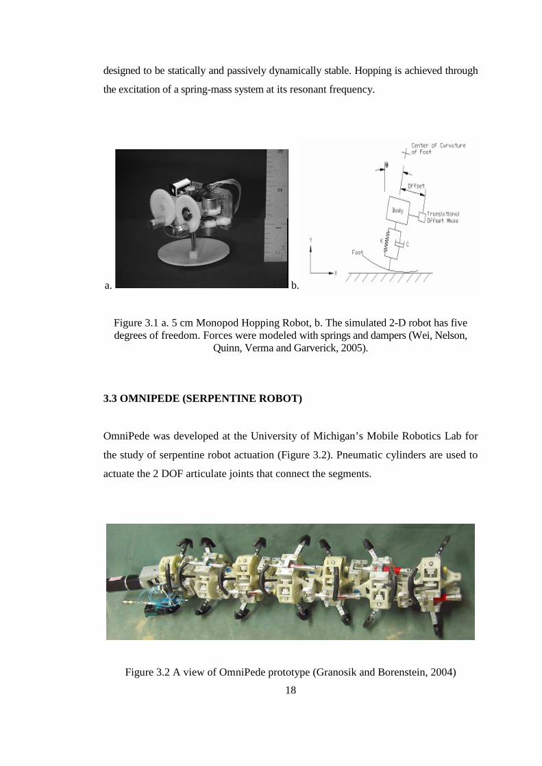
OmniPede was developed at the University of Michigan’s Mobile Robotics Lab for
the study of serpentine robot actuation (Figure 3.2). Pneumatic cylinders are used to
actuate the 2 DOF articulate joints that connect the segments.
Figure 3.2 A view of OmniPede prototype (Granosik and Borenstein, 2004)

19
3.4 A SMALL, INSECT-INSPIRED ROBOT
Mini-Whegs weights less than 90 g, but can run at over three body-lengths per
second and surmount 3.8 cm high obstacles. It incorporates fully independent
running and jumping modes of locomotion using mechanic power (Morrey, et.al,
2003). The controllable jumping mechanism allows it to leap as high as 18 cm
(Figure 3.3, (Lambrecht, Horchler, and Quinn, 2005)).
a.
b.
Figure 3.3 a. The jumping mechanism of Mini-Whegs in retracted (top) and released
(bottom) positions, b. Composite of video frames showing Mini-Whegs jumping high over a 9 cm barrier (Lambrecht, Horchler, and Quinn, 2005).

20
3.5 BIOMIMETIC HEXAPOD ROBOT
Based on the features of an agile insect, the American cockroach is worked on a six
legged robot with 58 cm length, 14 cm width, and 23 cm height (Figure 3.4). The
legs of the robot were designed with three segments; coxa, femur and tibia. Tarsus
and trochanter were ignored in this design. Each of joints between body-coxa, coxa-
femur and femur tibia is a simple hinge joint. The robot, biobot, is powered by
pneumatic actuators. Functional use of a single dual action cylinder provides
movement in two directions as shown in Figure 3.5. The cylinder generates either
flexion or extension of the next limb segment depending on which chamber is filled
with pressurized air. The robot is considerably heavy, 11 kg, in relation to its size
due to the weight of the valve (Delcomyn and Nelson, 2000).
a. b.
Figure 3.4 a. An American Cockroach, b. Biobot (Delcomyn and Nelson, 2000)
Figure 3.5 Working process of the pneumatic muscle (Delcomyn and Nelson, 2000)

21
3.6 CRICKET MICRO-ROBOTS
CWR University Cricket Micro-robot: Researchers at Case Western Reserve
University (CWRU) have developed three hexapod robots based on insects (Figure 3.6,
(Birch, Quinn, Hahm, et al., 2005; Birch, Quinn, Hahm, et al., 2000; Espenscheid,
Quinn, Beer and Chiel, 1993; Webb and Harrison, 2005)). Important features of these
robots are tabulated in Table 3.1 (Espenscheid, Quinn, Beer and Chiel, 1993).
Figure 3.6 Anatomy of the cricket micro-robot (Birch, Quinn, et al., 2005)
Table 3.1 CWRU Hexapod Robots features
Robots Based on DOF Controllers Size RI Stick insects 2 DOF in each leg
Neural Network Controller
Much larger than their animal models
RII Stick insects 3 DOF in each leg
Controllers were developed to enable insect-like gait movement
RIII Cockroach (Blaberus Discoidalis)
Hind legs; 3 DOF Middle legs; 4 DOF Front legs; 5 DOF
Complex Postural Controller
Much larger than their animal models

22
Cricket Cart Robot: Actuators, sensors and controllers were tested on this simple
legged platform, “Cricket Cart Robot”. It was constructed by mounting a pair of the
cricket robot’s rear legs on a wheeled cart as shown in Figure 3.7.
Figure 3.7 A view of the Cricket Cart Robot (Birch, Quinn, Hahm, Phillips, et al., 2005).
A Miniature Hybrid Robot Propelled by Legs: The autonomous hybrid micro-robot
uses its rear legs for propulsion and its front wheel help to support the body weight
(Figure 3.8). As a result, hybrid means that it uses both wheels and legs.
a. b.
Figure 3.8 a. A Hybrid robot, b. One leg of the hybrid robot (Birch, Quinn, et.al, 2005)

23
3.7 QUADRUPED JUMPING ROBOT
The robot was designed by legs which widely spread like spiders (Figure 3.9). The
legs are consisted of 4-bar linkages (Kikuchi, Ota et.al, 2003). Legs are controlled by
a pair of pneumatic cylinders as shown in Figure 3.10. It can jump only at the same
position; it protects its lateral position which is different from the first idea of
concept (Titech, 2006).
Figure 3.9 Locomotion Concept of Jumping Quadruped (Kikuchi, Ota et.al, 2003)
Figure 3.10 A view of Quadruped Jumping Robot (Titech, 2006)
24
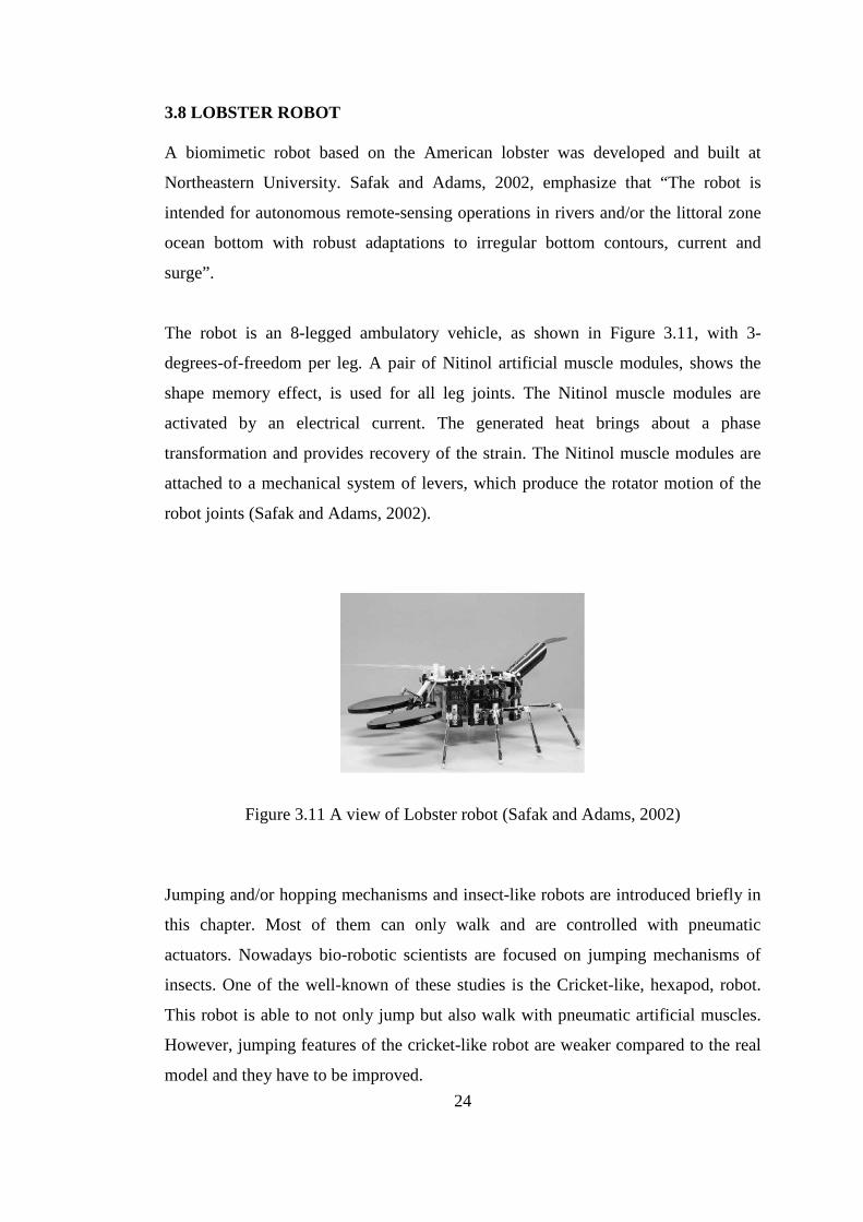
3.8 LOBSTER ROBOT A biomimetic robot based on the American lobster was developed and built at
Northeastern University. Safak and Adams, 2002, emphasize that “The robot is
intended for autonomous remote-sensing operations in rivers and/or the littoral zone
ocean bottom with robust adaptations to irregular bottom contours, current and
surge”.
The robot is an 8-legged ambulatory vehicle, as shown in Figure 3.11, with 3-
degrees-of-freedom per leg. A pair of Nitinol artificial muscle modules, shows the
shape memory effect, is used for all leg joints. The Nitinol muscle modules are
activated by an electrical current. The generated heat brings about a phase
transformation and provides recovery of the strain. The Nitinol muscle modules are
attached to a mechanical system of levers, which produce the rotator motion of the
robot joints (Safak and Adams, 2002).
Figure 3.11 A view of Lobster robot (Safak and Adams, 2002)
Jumping and/or hopping mechanisms and insect-like robots are introduced briefly in
this chapter. Most of them can only walk and are controlled with pneumatic
actuators. Nowadays bio-robotic scientists are focused on jumping mechanisms of
insects. One of the well-known of these studies is the Cricket-like, hexapod, robot.
This robot is able to not only jump but also walk with pneumatic artificial muscles.
However, jumping features of the cricket-like robot are weaker compared to the real
model and they have to be improved.

25
CHAPTER 4
MODELING AND ANALYSIS OF GRASSHOPPER-LIKE
JUMPING MECHANISM
Developing a biomimetic design requires careful focusing and modeling on the
biological domain to mimic the biological functions in engineering domain. Third
step of the biomimetic design is to develop a mathematical model and analyzing it on
the way of the biomimetic design tree. Equations of the leg models are developed by
the following steps;
a. A mathematical model description for the leg,
b. Kinematic analysis of the leg,
c. Dynamic analysis of the leg.
Two leg models, 2D and 3D, are developed in this chapter. Three structures, coxa,
trochanter, and tarsus, are ignored to reduce complexity of the models.
4.1 3D LEG MODEL
4.1.1 Mathematical Model Description for 3D Leg Model
Insects usually have many degrees of freedom. If bio-robots have degrees of freedom
as many as the real one has, they would be complicated mechanisms to analyze and
control. Although a robot may have many moving parts, these are all connected
together and execute a fixed cycle, which can be specified by a few parameters.
Consequently, reducing the number of degrees of freedom to a manageable level is
necessary to analyze leg structures easily.

26
Ways of managing complexity may be summarized as follows;
1. Reducing the number of DOF; analytically, by finding approximations,
constraints and by designing machines with the minimum number of joints.
2. Splitting a complex problem into several simpler ones by, for example,
separating the control of quantities which do not interact significantly.
A leg model is developed with 2 segments instead of 5 segments in the actual model
and the model has 3 degrees of freedom (DOF). Trochanter, coxa and tarsus
structures are ignored for not only 2D of leg model but also 3D of leg model.
4.1.2 Kinematic Analysis for 3D Leg Model
There are two joints in the 3D model; body-femur and femur-tibia, and there are also
three angles; femur- tibia angle, )(tα , and body-femur angles, β(t) and γ(t) as shown
in Figure 4.1. The position of centre of mass is represented as x, y, and z and can be
expressed in terms of the femur length, L1, and the tibia length, L2, as;
27.0))()(sin()).(cos(.))(sin()).(cos(.)( 21 +−−= tttLttLtx αβγβγ (4.1)
42.2))(sin()).()(cos(.))(sin()).(cos(.)( 21 +−−= tttLttLty γαβγβ (4.2)
))()(cos()).(cos(.))(cos()).(cos(.)( 21 tttLttLtz αβγβγ −+−= (4.3)
Figure 4.1 The grasshopper (Pholidoptera) leg model (CM: Centre of Mass)

27
According to the published experimental data L1=17.1 mm, L2= 15.6 mm (Table 4.1,
(Burrows and Morris, 2003)). To prevent complexity of the robot and reducing the
number of degrees of freedom to a manageable level the rear legs also froze the
active )(tγ joint at 30°. )(tα and z(t) are taken from the experimental data of Burrow
and Morris, given in Figure 4.2.
Table 4.1 Experimental data (Burrows and Morris, 2003) used for jumping simulation
Total body mass (M) 415 mg Hind leg tibia length (Ltibia) 15.6 mm Hind leg femur length (Lfemur) 17.1 mm Hind leg femur max.-min. diameter (D1- D2) 3.2-0.8 mm Tibia tubular construction diameter (D3) 0.6 mm Extensor muscle occupying a cross-sectional area 4.4 mm2 Flexor muscle occupying a cross-sectional area 1.08 mm2 Angle of rotation of tibia 165°
Body Structure
Lump Thickness 130 µm Horizontal distance (d) 302 mm Take-off angle (α) 33.8 deg Potential Energy (Ep) 20µJ
Jumping Performance
Co-contraction time (ms) 50-250 Density coefficient of leg material (ρ) 1.025 kg/m3
Figure 4.2 The changes in the Femur-Tibia angle, body height and velocity of body movement during a jump by a Pholidoptera male (Burrows and Morris, 2003).

28
Body height and femur-tibia angle changes are assumed to be zero in the interval
between -80 ms to -20 ms, so the changes can be ignored. Hence, the body height
(z(t)) and Femur-Tibia angle ( )(tα ) can be represented analytically by using the
empirical data obtained from the Figure 4.3 where -20 ms are shifted to origin for
using positive time in equations. The formulae are tabulated in the Table 4.2 for a
positive time interval to be used in the kinematical analysis.
a. b.
Figure 4.3 a. Body height (z(t)), b. Femur-Tibia angle ( )(tα ) of real body movement of a Pholidoptera male before take-off for positive time definite.
Table 4.2 Body height and femur tibia angle parabolic curves according to a time interval.
Time (t (ms)) 200 ≤≤ t
body height (z(t) (mm)) 50501833.0018305.000332333.0 23 +++− ttt
femur-tibia angle(α (deg)) 2026666675.0026.000133333.0 23 +++ ttt
29
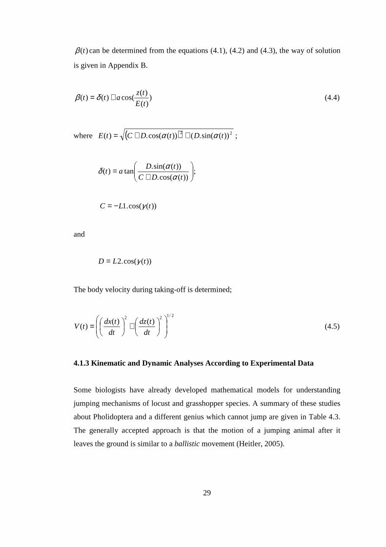
)(tβ can be determined from the equations (4.1), (4.2) and (4.3), the way of solution
is given in Appendix B.
))(
)(cos()()(
tE
tzatt += δβ (4.4)
where ( ) 22 ))(sin(.())(cos(.)( tDtDCtE αα ++= ;
+=
))(cos(.
))(sin(.tan)(
tDC
tDat
ααδ ;
))(cos(.1 tLC γ−=
and
))(cos(.2 tLD γ=
The body velocity during taking-off is determined;
2/122)()(
)(
+
=dt
tdz
dt
tdxtV (4.5)
4.1.3 Kinematic and Dynamic Analyses According to Experimental Data
Some biologists have already developed mathematical models for understanding
jumping mechanisms of locust and grasshopper species. A summary of these studies
about Pholidoptera and a different genius which cannot jump are given in Table 4.3.
The generally accepted approach is that the motion of a jumping animal after it
leaves the ground is similar to a ballistic movement (Heitler, 2005).
30
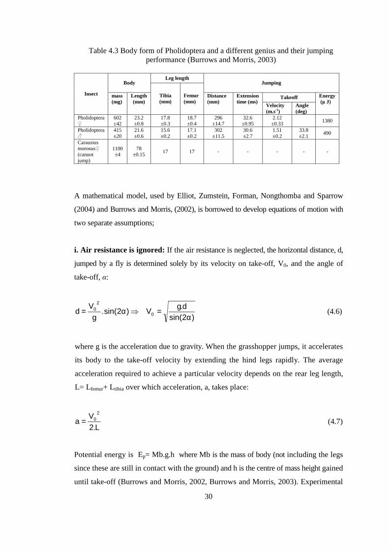
Table 4.3 Body form of Pholidoptera and a different genius and their jumping performance (Burrows and Morris, 2003)
Leg length
Body Jumping
Takeoff Insect mass
(mg) Length (mm)
Tibia (mm)
Femur (mm)
Distance (mm)
Extension time (ms)
Velocity (m.s-1)
Angle (deg)
Energy (µ J)
Pholidoptera♀
602 ±42
23.2 ±0.8
17.8 ±0.3
18.7 ±0.4
296 ±14.7
32.6 ±0.95
2.12 ±0.33
1380
Pholidoptera ♂
415 ±20
21.6 ±0.6
15.6 ±0.2
17.1 ±0.2
302 ±11.5
30.6 ±2.7
1.51 ±0.2
33.8 ±2.1
490
Carausius morosus♀ (cannot jump)
1100 ±4
78 ±0.15
17 17 - - - - -
A mathematical model, used by Elliot, Zumstein, Forman, Nongthomba and Sparrow
(2004) and Burrows and Morris, (2002), is borrowed to develop equations of motion with
two separate assumptions;
i. Air resistance is ignored: If the air resistance is neglected, the horizontal distance, d,
jumped by a fly is determined solely by its velocity on take-off, V0, and the angle of
take-off, α:
⇒α= )2sin(.g
Vd
20
)2sin(d.g
V0 α= (4.6)
where g is the acceleration due to gravity. When the grasshopper jumps, it accelerates
its body to the take-off velocity by extending the hind legs rapidly. The average
acceleration required to achieve a particular velocity depends on the rear leg length,
L= Lfemur+ Ltibia over which acceleration, a, takes place:
L.2V
a2
0= (4.7)
Potential energy is Ep= Mb.g.h where Mb is the mass of body (not including the legs
since these are still in contact with the ground) and h is the centre of mass height gained
until take-off (Burrows and Morris, 2002, Burrows and Morris, 2003). Experimental

31
data of Burrows and Morris, 2002, given in Table 4.1, are considered in the
computation. Thus, the height gained until take-off can be calculated after determining
the mass of the body without legs. The mass of the femur can be calculated as two
cylinders with diameters 3.2 mm and 0.8 mm and lengths 10.26 mm and 6.84 mm,
respectively. Tibia is also taken as a cylinder with 0.6 mm in diameter. Therefore, the
mass of the body and initial height of body can be found easily by using these
assumptions.
ii. Air resistance is not ignored: Air resistance is an important energy loss for small
insects so that the actual kinetic energy at take-off is larger than the kinetic energy
without air resistance. In order to estimate the actual kinetic energy at take-off,
Elliott, et al, (2004) observed Drosophila (from which the wings had been removed)
moving vertically upwards in air and in vacuum. 20% of the energy was reported to
be lost to air resistance for flies projected upwards 100 mm. If the assumption is that
the same loss occurs in the experiments, the kinetic energy at take-off, allowing for
air resistance ( airkE , ), will be 1.25 times higher than the energy required without air
resistance. This would require the take-off velocity to be increased by 25.1 (Elliott, et
al, 2004).
4.2 2D LEG MODEL
4.2.1 Mathematical Model for 2D Leg Model
A two-actuator model having 2 DOF is considered in the analysis. Model consists of
three links and two actuators, one at hip joint and another at knee joint as seen in the
Figure 4.4. Although the model is a very simplified one, it will help in determining
optimum parameters for a higher degree of freedom system.

32
Figure 4.4 2D Leg Model
4.2.2 Kinematic Analysis
The position of centre of mass is given for hip-knee joint actuators model;
27.0))(sin(..866.0))(sin(..866.0)( 21 +−= tLtLtx θβ (4.8)
))(cos(..866.0))(cos(..866.0)( 21 tLtLtz θβ +−= (4.9)
where )()()( ttt αβθ −=
Similar results for the femur-tibia angle with 3-D Leg Model are achieved. Way of
the 2-D solutions is given in the Appendix C. The leg motion according to these
results is given in the Figure 4.5.

33
Figure 4.5 Position of a grasshopper leg until take-off
4.2.3 Dynamic Analysis
The very first step in dynamic analysis is to develop a dynamic model. Mass
distribution is given in the Figure 4.6.
Figure 4.6 Mass distribution of the leg model

34
M1 and M2, limb masses, are concentrated at the mid points of the limbs. Mk
represents the mass of the knee actuator and Mh is hip actuator mass. Mb is the body
mass and it is concentrated at the centre of mass of the body. I1, I2 and Ib are the
moments of inertia of the limbs about their centroids;
12
1.11
2LMI = and
12
2.22
2LMI = (4.10)
To find the limb mass, models of the femur and tibia are given in the Appendix D.
mgmmkgVM femur 0881.0)()10.(958.85)./(025.1.1 3333 ≅== −ρ (4.11)
mgmmkgVM tibia 00452.0)()10.(41.4)./(025.1.2 3333 ≅== −ρ (4.12)
Consequently, bM the mass of body (not including the legs) becomes
mgmMMMM legsb 65.414.4)21.(2 =−+−= (4.13)
where legsm is front legs weight and it is assumed that legsm =0.04 mg according to
experiments and total mass, M , is about 415 mg. Note that the grasshoppers have
six legs; two of them are hind legs. A Lagrange’s method is used for arriving at
equations between joint power and foot coordinates. Elaboration solution is given in
the Appendix E.
i. Using Lagrange’s Method, the Torque for Knee Actuator is;
542
3212 ))(()()(. GgGtGtGtGT ++++= ββθ &&&&& (4.14)
where

35
22
211 ).)(75.0( ILMMMMG kbh ++++= (4.15)
))()(cos())(75.0375.0( 2112 ttLLMMMG bh θβ −++−= (4.16)
))()(sin())(75.0375.0( 2113 ttLLMMMG bh θβ −++= (4.17)
))(sin()5.0( 2124 tLMMMMMG bhk θ++++= (4.18)
))()((5 ttkG βθ −= (4.19)
ii. Using Lagrange’s Method, the Torque for Hip Actuator is;
572
33621 ))(()()(2)()(. GgGtGttGtGtGT −+−++= θθββθ &&&&&&& (4.20)
where
12
116 ).)(75.0188.0( ILMMMMG kbh ++++= (4.21)
))(sin()5.0( 117 tLMMMG bh β++−= (4.22)
4.3 RESULTS OF THE 2D AND 3D LEG MODEL
Variations of angles )(tα , )(tγ , )(tθ ( )(tθ =β(t) - )(tα ), and β(t) (rad) are given in
the Figure 4.7, the position of centre of mass during take off is given in the Figure
4.8, and the body velocity is plotted in the Figure 4.9. The body height variations
according to horizontal distance are plotted in Figure 4.10 to see the path of the
centre of mass. All body height and femur-tibia angle values are compared with the
numerical solutions via Mathcad 2000 program. The solution is given in Appendix
A. Consequently, it is obtained that the found values are similar of the empirical data
of Burrows and Morris, (2003).

36
Figure 4.7 Variations of Femur-Tibia, Body-Femur, and Ground-Tibia angles until take-off
Figure 4.8 Variations of position of centre of mass coordinates until take-off

37
Figure 4.9 A plot of velocity until take-off
Figure 4.10 A body height variation along horizontal distance until take-off

38
4.4 RESULTS OF THE TORQUE ANALYSIS OF THE 2D LEG MO DEL
The torque values based on 2D leg model are tabulated in Appendix F. The data given
in Table F.1 are graphically shown in Figure 4.11 and Figure 4.12. The variation of
torque is very small because knee actuator and hip actuator cancel each other due to
their signs and magnitudes.
Figure 4.11 A graph of time-torque variation of 2D leg model where T is the total torque; T1 is the hip actuator torque; T2 is the knee actuator torque
Figure 4.12 Total torque of 2D leg model

39
4.5 KINEMATIC ANALYSIS OF 3D LEG MODEL WITH MSC. AD AMS
SIMULATION
MSC. Adams simulation software is used to obtain results of the jumping based on
the presented mathematical model. In this simulation, the grasshopper given in the
Figure 4.13 is assumed to be a sphere which has the same weight and parameters
with the actual model.
The horizontal and vertical distances, kinetic energy and velocities are calculated by
MSC. Adams analyses and the results are given in Figure 4.14 and Figure 4.15.
When the results in Table 4.4 are compared to each other, it is apparent that they are
close for different cases. The similarity of the results shows the validity of the
simplifying assumptions.
Figure 4.13 A grasshopper is modeled by using MSC. Adams Simulation Program

40
Figure 4.14 Displacement analysis of grasshopper-like by using MSC. Adams 2005
a.
b.
Figure 4.15 Like-grasshopper jumping analysis by using MSC. Adams 2005 r2 a. Velocity Analysis, b. Kinetic energy analysis.

41
The results for the cases considering air resistance and without air resistance are used to
obtain the numerical data tabulated in Table 4.4. The results are compared with
experimental data of Burrows and Morris, (2003) for understanding the difference
between the assumptions to get hold of jumping performance of Pholiptera.
Table 4.4 Jumping performance data of Pholiptera motion
Experiment (Burrows and Morris, 2002)
Air resistance is
ignored
Force is constant with air resistance
Adams Solution
Take-off velocity (m/s) 1.51 1.79 2 Input data
(1.79) Take-off time (s) - - - 0.203 Take-off acceleration (m/s2) - 48.99 61.2 -
Peak acceleration (m/s2) 83.4 97.98 122.32 -
Take-off force (Mn) - 20.3 25.6 -
Extension time (ms) 30.6 36.5 30 -
Horizontal distance (mm) Input data (302)
Input data (302)
Input data (302) 301.861
Height gained until take-off(mm)
- 4.92 4.92 -
Kinetic Energy (µJ) 470 614.74 768.43 664.1
Min. Energy requirement (µJ)
490 634.74 788.43 684.1
Power (µW) 16 36.3 51.2 -
In this chapter, mathematical models are studied according to the biomimetic design
tree. 2D and 3D models are developed and take-off angles are estimated. Although
there are two different models, the angles are close to each other and that of
biological model. Hind leg position until take-off is evaluated with the take-off
angles. Artificial muscle stroke can be obtained with this data.
Several assumptions are made for reducing the complexity. A femur-body
angle, )(tγ , is assumed to be 30°. This angle variation can be added to the model as a
future work. Moreover, torque analysis, using Lagrange’s method, is developed.
Force analysis of leg models of artificial muscles and biological muscles will be
observed according to torque analysis of the hind leg. In addition to these analyses, a
packet simulation program, MSC. Adams, is applied basically to concluding the
jumping features of real model. All of results are used for evaluation of artificial
model and preliminary design.

42
CHAPTER 5
ARTIFICIAL MUSCLES AND
DEVELOPMENT OF A NEW ARTIFICIAL MUSCLE
The main scope of this thesis is to create a basic system that mimics aspects of the
jumping mechanism of a grasshopper instead of creating models with complex
structures. Better actuation and sensing technology effects the development of basic
biomimetic robot structures critically (Biomimetic, 2006).
Natural muscle is a contractile organ and a simply transducer. They change the
chemo-electric signal from nerves to mechanical energy. Fibers, consisted by
muscles, actuate force and motion in response to nervous stimulation (Brabham,
Marr, Smith and Lee, 2004).
Fourth step of the biomimetic design is an abstraction of good actuator system from
biological muscles. Since the natural muscles are non-fabricated structures and they
cannot be copied completely, the study of artificial muscles is the most difficult part
of this study. After the literature survey on artificial muscles, a new artificial muscle
is developed.
5.1 LITERATURE SURVEY ON ARTIFICIAL MUSCLES
O’Halloran and O’Malley, (2004) described that “Mammalian skeletal muscle is an
incredibly elegant mechanism. Muscle is a three dimensional nanofabricated system
with integrated sensors, energy delivery, waste/heat removal, local energy supplies,
actuator, and repair mechanisms”. Although natural muscle has a non-fabricated
character, actuators and actuator systems are essential features of all robots,

43
providing the forces, torques and mechanical motions needed to move the joints,
limbs or body (Caldwell, Medrano-Cerda, and Goodwin, 1994). Thus, research
projects with huge budgets are funded for mimicking natural muscles.
There is an example of using real muscle tissue frog-like robot (Figure 5.1). In this
design, using very simple control and interface design, muscles can act as a practical,
controllable actuator, but this muscle tissue requires a special medium to be alive. To
use such a biological muscle tissue is technologically not practical and moreover it is
not sufficient for robotic applications, so an artificial muscle is necessary.
Figure 5.1 A Swimming Robot Actuated by Living Muscle Tissue (H: rigid Delrin head piece; D: rigid Delrin backbone; M: muscle; B: lithium batteries; C:
encapsulated microcontroller, infra-red sensor, and stimulator unit; T: cast silicone tail; F: Styrofoam float; w: electrode wires; s: suture attachments; k: compliant hinge
segment; a: cylindrical tail mounting boss) (Huge Herr, Robert, 2004)
44
Industrial robots usually use three primary power sources;
- Electric motors
- Hydraulic cylinders
- Pneumatic cylinders (Caldwell, Medrano-Cerda, and Goodwin, 1994).
Though electric motors have a very important and common place in robotic
application areas because they are very easy to control, for example Honda's
humanoid Asimo (Brown, 2004), they have some disadvantages. Firstly, motors are
heavy for robotic applications. The other disadvantage is that their force-to-weight
ratio is lower than that of pneumatic and hydraulic devices (Kapps, 2007). Moreover,
this actuator type is not sufficient for biomimetic design approach.
Pneumatic (Kerscher, Albiez, and Berns, 2002) and hydraulic cylinder systems
eliminate some of the problems associated with electric motors. These actuators also
produce linear motion, which makes them more suitable to serving a role equivalent
to muscle (Kingsley, 2005). However, these actuators have standard size which is too
big and heavy for micro-robots.
Entire soft body is one of the essentials for robots (Lee, Shimoyama, 2002). Thus,
the actuator problem is seemed to solve by soft artificial muscles (Kerscher, Albiez,
and Berns, 2002). Their performance is characterized by (Caldwell, et. al, 1994);
- Power (in particular the power/weight and power/volume ratios)
- Strength
- Response rate
- Physical size
- Speed of motion
- Reliability
- Controllability
- Compliance
- Cost
- etc…

45
Although soft actuators have been considered recently, a number of new different
type of technologies have been developed (Caldwell, Medrano-Cerda and Goodwin,
1994) and most of them are compared in Table 5.1 (Arora, 2005).
Table 5.1 Comparison of natural muscle and man-made actuator technologies (Arora, 2005; Pelrine, Kornbluh, Pei, et. al, 2002)
5.1.1 Braided Pneumatic Actuators (BPA); McKibben Artificial Muscles; Air
Muscles
“One of the earliest attempts at artificial muscle modeling was undertaken by an
American physician, McKibben in the 1950’s Pneumatic actuators were one of the
first approaches to artificial muscle modeling”, O’Halloran and O’Malley, (2004).
Air muscles are soft pneumatic devices, ideally suited for robotics and bio-robotics.
In addition to this their positive characters, they have similar features with rear
muscles (Figure 5.2).

46
Figure 5.2 The force-length relationship of Braided Pneumatic Actuator’s compared to that of muscle (Fm: Muscle force; Fm,o: Initial muscle force; Lm: Muscle length,
Lm,o: Initial muscle length, (Kingsley, 2005; Colbrunn, 2000))
Braided Pneumatic Actuator (BPA), which have applications in robotics, bio-
robotics, biomechanics, artificial limbs replacement and industry, consists of a rubber
bladder encompassed by a tubular braided mesh (Figure 5.3.a). When the bladder is
inflated, the actuator expands radial and undergoes a lengthwise contraction (Figure
5.3b and Figure 5.4). Typically air muscles can contact up to twenty five percentage
of their elongated length (Biorobotic, 2006). Pneumatic actuators success is depend
on compressors because the simple system uses a small air pump or compressor,
which are driven by electric motors.
a. b.
Figure 5.3 A view of BPA a. a braided pneumatic actuator (Kingsley, 2005) b. An inflated (bottom) and uninflated (top) actuator (Colbrunn, 2000)

47
Figure 5.4 Working mechanism of a pneumatic muscle (Biorobotic, 2006).
Pneumatic cylinders (Granosik and Borenstein, 2004);
� are clean and lightweight,
� have large power output,
� have relatively low cost.
The hybrid micro robot uses braided pneumatic actuators, McKibben artificial
muscles, to extend the leg segments (Figure 5.5). This robot features are given in the
literature survey of bio-robots, Chapter 3.
Figure 5.5 Case Western University Hybrid Robot with rear leg, its actuator is a McKibben Artificial muscle (Birch, et al., 2005)

48
A robotic leg, which has four degrees of freedom, was used to conclude control
mechanism of braided pneumatic actuators. This leg can swing, stance and walk
across a table. The hardware system and leg design are given in Figure 5.6.
a. b.
Figure 5.6 a. The hardware system of a leg design model, b. the leg model (Colbrunn, 2000)
5.1.2 Shape Memory Alloys (SMA)
Shape memory was discovered in 1932 and Nickel-Titanium alloys were found to
exhibit shape memory significantly at Naval Ordinance Labs in 1962 (Virtualskies,
2007). SMA, a group of metallic materials, contracts with a thermal cycle (Lowe,
2006). SMAs contact up to ten percentage of their elongated length when heated and
they return to their original length when cooled off (O’Halloran and O’Malley, 2004
(Figure 5.7)). Shape-Memory alloys can tolerate strain 3 to 25 times higher than
piezoelectric can.

49
Figure 5.7 Basic Principles of SMA (Kapps, 2007)
Some Shape-Memory alloys:
• nickel-titanium (Nitinol),
• gold-cadmium,
• gold-cadmium,
• brass,
• ferromagnetic (a thin film, low bandwidth alloy).
They are sometimes inadequate although SMAs have advantages (Kapps, 2007);
- can recover from large amounts of bending and torsion,
- possess an extremely high force to weight ratio,
- are incredibly compact and simple,
- are pseudo-elasticity material (or sometimes called super elasticity, a
pseudoelastic material may return to its previous shape after the removal of
even relatively high applied strains.)
50
Disadvantages of SMAs;
- are unable to produce significant size displacement (only about 4-10%),
- are inefficient ( only about 10% due to heating),
- are difficult to model (due to non-linear qualities in actuations),
- are somewhat expensive to manufacture,
- have relatively slow reaction time.
As a result of the fact that SMAs requires small space, have various forms; wires,
tubes, sheets, etc. for using different application areas, and they have less weight than
a conventional actuator, they are highly useful in situations where conventional
actuators are too large, bulky, or inadaptable (Kapps, 2007). Six-legged robot, based
on a spider insect, is an example of a bio-robot which is controlled with shape
memory alloys to yield a walking motion. Legs contract when heat energy is
increased and the legs expand when the material cools. Other examples of bio-robots
which are used Shape Memory Alloys are a winged robot whose wings expand and
contract to produce a flight motion, a fish robot that swims, and a snake robot that
slithers (Virtualskies, 2007).
5.1.3 Electroactive Ceramics (EAC)
Polycrystalline ceramics are an example of Electroactive ceramics. Application of a
high electric field at an elevated temperature is used as part of the poling process to
align the microscopically small piezoelectric domains (Figure 5.8, (O’Halloran and
O’Malley, 2004)).

51
a. b. c.
Figure 5.8 Polarisation is a result of the alignment of piezoelectric domains a. disk after polarization, b. applied voltage same polarity as poling voltage: disk lengthens, c. applied voltage opposite polarity as poling voltage: disk contracts (O’Halloran and
O’Malley, 2004).
5.1.4 Electromagnetic
Lowe, (2006) represents that “Electromagnetic solutions typically consist of a motor
that rotates an output shaft; it connects to a drive train, gear reducer transmission or
other mechanical device that has several touching and moving parts, which create an
indirect displacement”.
5.1.5 Piezoelectric
Piezoelectric (piezo means pressure in Greek) effect was discovered by the Curic
brothers in the 1880’s (Stilson, 1996). If piezoelectric materials are hit with electric
current, they deform; they generate electricity if they are deformed. Namely,
mechanical stress causes crystals to electrically polarize and vice versa (Ashley,
2003). Piezoelectric technologies expand and contract with voltage at high
frequencies (Lowe, 2006). In contrast, piezoelectric materials can generate large
stress of about 10-40 MPa, but this force gives only a few nanometers. Piezoelectric
actuators (Kapps, 2007);
- are very fast,
- require high voltages,
- are very accurate,
- have high repeatability,
- return to their resting state when the electric stimulus is removed,
- can withstand very broad temperature ranges.

52
5.1.6 Electroactive Polymer Artificial Muscle (EAP or EPAM)
Since the early 70’s a new Electroactive polymer materials has grown, but the most
progress was made after 1990. Drive robots with more efficient, higher power
density actuation was discovered due to a new technology muscle, called
Electroactive Polymer Artificial Muscle (EPAM or EAP), in the early 1990's (Figure
5.9). An EAP actuator is not only completely different from conventional electro-
mechanical devices, but also separates itself from other high-tech approaches that are
based on piezoelectric materials or shape-memory alloys by providing a significantly
more power-dense package (Lowe, 2006; Ducheon, 2005). Energy density of
actuators is given in Figure 5.10 where EM represents electro-mechanical devices.
Figure 5.9 A view of EAP, EPAM Roll Actuator from Artificial Muscle (Lowe, 2006).
Figure 5.10 EAP actuators-energy density/frequency characteristics (Ducheon, 2005)

53
Electroactive polymers are resembled human muscles because EAPs expand and
contract silently, based on variable voltage input levels (Prnewswire, 2006; Bar-
Cohen, 2005) and they have high fracture toughness, large actuation strain and
inherent vibration damping (O’Halloran and O’Malley, 2004). In contrast EAPs have
a much smaller and lower weight form factor than Electromagnetic (EM) motor
devices, much like the human muscle, but they provide the same level of power as
EM devices (Ducheon, 2005). Elements of EAP actuated devices and principle of
operation is given basically in Figure 5.11. EAPs (Kapps, 2007),
- can induce strains (at least twice greater in magnitude than EACs),
- have higher response speeds, lower densities and improved resilience than
SMAs,
- have low mechanical energy density,
- have low actuation forces.
Figure 5.11 Principle of operation EAP actuated devices (Bar-Cohen, 2000).
Types of EAPs
EAPs can be sorted into two groups: ionic EAPs and electronic EAPs are given in
Appendix G, Table G.1. Each of them is compared with advantages and
disadvantages. Applications areas and devices of these EAPS are tabulated in
Appendix G, Table G.2.

54
1. Ionic EAP;
Ionic polymer gels (Figure 5.12), ionomeric polymer-metal composites (IPMC,
(Figure 5.13)), conductive polymers carbon nanotubes and electrorheological fluids,
work on the basis of electrochemistry- the mobility or diffusion of charged ions are
examples of Ionic EAPs (IEAP). They need not only a current to hold position but
also wet media or flexible coating (Lowe, 2006; Ashley, 2003). IEAP materials are
generally used in robotics, biotechnology and industrial applications (Shahinpoor,
Kim, 2004). Multifinger grippers, an example of IPMC (Figure 5.13.b), have a great
mass carrying capability (Bar-Cohen, Xue, Joffe, Lif, Shahinpoor, Simpson, Smith,
and Willis, 1997). Properties of all variety of ionic EAP are tabulated according to
Bar-Cohen, 2005 in Appendix G, Table G.1.
a. b.
Figure 5.12 A view of Ionic EAPs, a. Ionic gel at reference state, b. activated state (O’Halloran and O’Malley, 2004; Bar-Cohen, 2004).
a. b.
Figure 5.13 a. An illustration of the IPMC gripper concept, b. a four-finger gripper (Shahinpoor, Kim, 2004)

55
2. Electronic EAPs;
Electronic EAPs, such as ferroelectric polymers (Figure 5.14.a), electrets, dielectric
elastomers (Figure 5.14.b) and electrostrictive graft elastomers (Figure 5.14.c), are
driven by electric fields. Although electronic EAPs do not need a protective coating
and required almost no current to hold position, and electronic EAPs can react
quickly and deliver strong mechanical forces, they require relatively high voltages,
which can cause uncomfortable electric shocks (Lowe, 2006; Ashley, 2003).
Properties of all variety of electronic EAP are tabulated according to Bar-Cohen,
2005 in Appendix G.
a.
b.
c.
Figure 5.14 Electronic EAPs a. Ferroelectric polymer in the reference state (left) and in its actuated state (right), b. circular strain test of a dielectric elastomer with carbon
grease electrodes, c. electrostrictive graft elastomer (O’Halloran and O’Malley, 2004).

56
Dielectric EAP, an Electronic EAPs Type,
An important type of Electronic EAPs is dielectric EAP whose basic architecture is
made up of a film of an elastomer dielectric material that is coated on both sides with
another expandable film of a conducting electrode. When voltage is applied to the
two electrodes a Maxwell Pressure (Ducheon, 2005) is created upon the dielectric
layer. Electrode pressure causes the dielectric film to become thinner; it expands in
the planar directions. Thus, electrical force is converted to mechanical actuation and
motion (Figure 5.15, (Ashley, 2003; Ducheon, 2005; Lowe, 2006)).
Figure 5.15 Working mechanism of Dielectric EAP (Ashley, 2003)
Dielectric elastomers can generate more strain and force than many of the competing
technologies (Ashley, 2003) and they are sensitive their position, so Dielectric EAPs
do not require a dedicated position sensor (Kapps, 2007). Their properties in this
regard are similar to those of natural animal muscle (Figure 5.16). Another advantage
of this type is that dielectric elastomer actuators require relatively high voltages (1-5
kV) to active, so devices can operate at a very low current. They also use thinner,
less expensive wiring and keep fairly cool (Ashley, 2003).
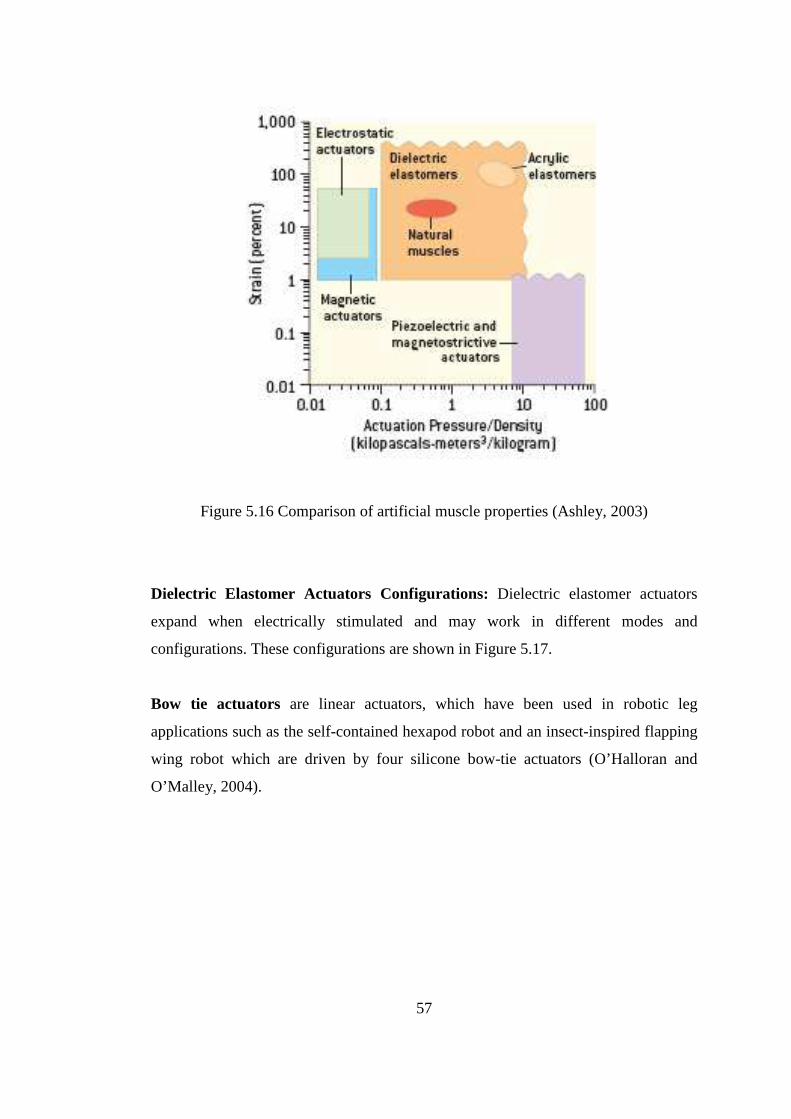
57
Figure 5.16 Comparison of artificial muscle properties (Ashley, 2003)
Dielectric Elastomer Actuators Configurations: Dielectric elastomer actuators
expand when electrically stimulated and may work in different modes and
configurations. These configurations are shown in Figure 5.17.
Bow tie actuators are linear actuators, which have been used in robotic leg
applications such as the self-contained hexapod robot and an insect-inspired flapping
wing robot which are driven by four silicone bow-tie actuators (O’Halloran and
O’Malley, 2004).
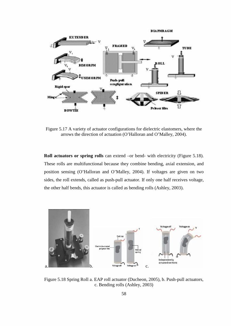
58
Figure 5.17 A variety of actuator configurations for dielectric elastomers, where the arrows the direction of actuation (O’Halloran and O’Malley, 2004).
Roll actuators or spring rolls can extend –or bend- with electricity (Figure 5.18).
These rolls are multifunctional because they combine bending, axial extension, and
position sensing (O’Halloran and O’Malley, 2004). If voltages are given on two
sides, the roll extends, called as push-pull actuator. If only one half receives voltage,
the other half bends, this actuator is called as bending rolls (Ashley, 2003).
a. b. c.
Figure 5.18 Spring Roll a. EAP roll actuator (Ducheon, 2005), b. Push-pull actuators,
c. Bending rolls (Ashley, 2003)
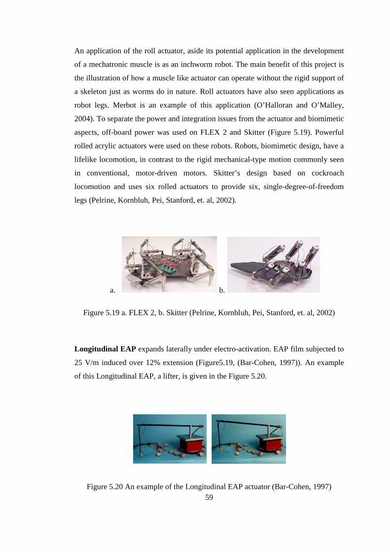
59
An application of the roll actuator, aside its potential application in the development
of a mechatronic muscle is as an inchworm robot. The main benefit of this project is
the illustration of how a muscle like actuator can operate without the rigid support of
a skeleton just as worms do in nature. Roll actuators have also seen applications as
robot legs. Merbot is an example of this application (O’Halloran and O’Malley,
2004). To separate the power and integration issues from the actuator and biomimetic
aspects, off-board power was used on FLEX 2 and Skitter (Figure 5.19). Powerful
rolled acrylic actuators were used on these robots. Robots, biomimetic design, have a
lifelike locomotion, in contrast to the rigid mechanical-type motion commonly seen
in conventional, motor-driven motors. Skitter’s design based on cockroach
locomotion and uses six rolled actuators to provide six, single-degree-of-freedom
legs (Pelrine, Kornbluh, Pei, Stanford, et. al, 2002).
a. b.
Figure 5.19 a. FLEX 2, b. Skitter (Pelrine, Kornbluh, Pei, Stanford, et. al, 2002)
Longitudinal EAP expands laterally under electro-activation. EAP film subjected to
25 V/m induced over 12% extension (Figure5.19, (Bar-Cohen, 1997)). An example
of this Longitudinal EAP, a lifter, is given in the Figure 5.20.
Figure 5.20 An example of the Longitudinal EAP actuator (Bar-Cohen, 1997)

60
5.1.7 Antagonistically-Driven Linear Actuator (ANTL A)
ANTLA, based on dielectric elastomer, has bidirectional actuation, “push-pull” type
operation (Figure 5.21). ANTLA is a cost effective muscle because its fabrication
process is very simple. The advantages of this actuator are high force-to-weight ratio,
cost effectiveness, ease of fabrication, intrinsic softness, and disposability. Their
properties in this regard are similar to those of natural animal muscle (Choi, Jung,
Ryew, Nam Jeon, Koo, and Tanie, 2005)
Figure 5.21 Mechanical structure of ANTLA (Choi, Jung, Ryew, et.al, 2005)
5.1.8 Baughman and Colleagues’ Artificial Muscles
Methanol-powered artificial muscles have been created aiming to create battery-free
robotic limbs and prosthetics. Baughman and colleagues have designed two types of
artificial muscle that also act as fuel cells– converting chemical energy to mechanical
movement (Merali, 2006).
- A nickel-titanium shape-memory wire coated in a platinum catalyst.
- Sheets of carbon nanotubes, coated in a catalyst.

61
5.1.9 A Comparison of Artificial Muscles
Some important artificial muscles are considered in this part. The chronological
order of invention of an actuator and a few artificial muscles is given in Figure 5.22.
EAPs and pneumatic artificial muscles are the most efficient artificial muscles for
biomimetic design and their properties are much like natural muscles. In this scope,
EAPs, a new artificial muscle technology, and pneumatic artificial muscles are
studied particularly. The maximum stress-strain and maximum strain-power
characteristics of the actuators are given in Figure 5.23 and Figure 5.24.
Past 1831 1880 1950 1962 1990 Future
Ele
ctro
mec
han
ical
m
otor
P
iezo
elec
tric
Pne
umat
ic
S
MA
s
EA
Ps
Figure 5.22 Chronological order of invention of a few actuators/artificial muscles
“Current actuation technologies are based either on high modulus – low strain
materials, such as piezoceramics and magnetostrictors, or on multi-component
systems, such as hydraulic, pneumatic or electromagnetic devices”, Huber et.al,
(1997). Piezoelectric materials can generate large stress of about 10-40 MPa, but this
force gives only a few nanometers. It makes piezoelectric be a weak material as an
artificial muscle. Although shape memory alloys (SMAs) deliver both high forces
and large displacements, the response times and longevity of these materials require
optimization. EAPs systems are in the middle of the performance indices of
mechanical actuators, between the high stress-low strain and the low stress–high
strain groups. It is clear that dielectric elastomer has a higher strain-power ratio than
that of others and natural muscles have. Some important artificial muscles and a
natural muscle are compared with empirical data in Table 5.2 from different sources.

62
Figure 5.23 Max. Stress-Strain Graph for Actuator Materials. The sloping lines from left to right give an indication of the energy storage capacity per unit volume of the
various actuators (Bonser, Harwin, Hayes, et.al, 2004)
Figure 5.24 Actuator Max. Strain-Power Density Graph (Kapps, 2007)

63

64
5.2 STUDIES ON ARTIFICIAL MUSCLES
After literature survey on actuators and artificial muscles, the fourth step of the
biomimetic design, is considered, two ready-made artificial muscles are selected as a
grasshopper-like jumping mechanism actuator. The first alternative is an EAP muscle
whose properties are much like animal muscles. EAP muscles are soft actuators and
have high strain-stress ratios and high response speeds. Although it is seen that EAPs
is sufficient for the jumping mechanisms, this type is not used as an actuator for the
system because EAPs are new artificial muscles and their behavior is not known
properly for such a study. Because of the fact that EAPs require time for progress,
this type is not preferred for the mechanism as an actuator.
Another alternative is a pneumatic artificial muscle. The pneumatic artificial muscle
has a lot of advantages. Firstly, its physical characters are known exactly. The
muscle behaves like a spring with a changing external force: the displacement is in
direction of the applied force (Figure 5.25).
Figure 5.25 Pneumatic artificial muscle model (Festo, 2006)
Secondly, the contraction properties have similar features with biological muscles.
Other important features of the pneumatic artificial muscle are; light weight and
large power output, and low cost. In addition to these positive features, there is a
huge negative character; the ready-made pneumatic muscles size is too large. A
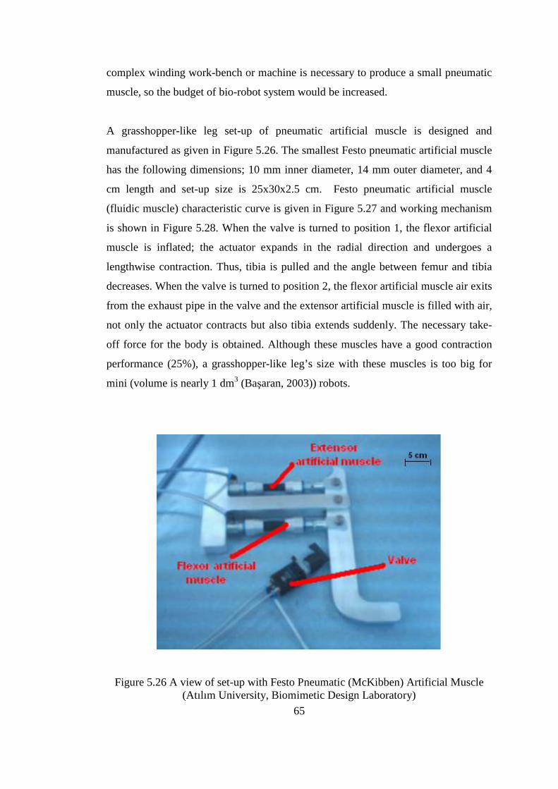
65
complex winding work-bench or machine is necessary to produce a small pneumatic
muscle, so the budget of bio-robot system would be increased.
A grasshopper-like leg set-up of pneumatic artificial muscle is designed and
manufactured as given in Figure 5.26. The smallest Festo pneumatic artificial muscle
has the following dimensions; 10 mm inner diameter, 14 mm outer diameter, and 4
cm length and set-up size is 25x30x2.5 cm. Festo pneumatic artificial muscle
(fluidic muscle) characteristic curve is given in Figure 5.27 and working mechanism
is shown in Figure 5.28. When the valve is turned to position 1, the flexor artificial
muscle is inflated; the actuator expands in the radial direction and undergoes a
lengthwise contraction. Thus, tibia is pulled and the angle between femur and tibia
decreases. When the valve is turned to position 2, the flexor artificial muscle air exits
from the exhaust pipe in the valve and the extensor artificial muscle is filled with air,
not only the actuator contracts but also tibia extends suddenly. The necessary take-
off force for the body is obtained. Although these muscles have a good contraction
performance (25%), a grasshopper-like leg’s size with these muscles is too big for
mini (volume is nearly 1 dm3 (Başaran, 2003)) robots.
Figure 5.26 A view of set-up with Festo Pneumatic (McKibben) Artificial Muscle (Atılım University, Biomimetic Design Laboratory)

66
Figure 5.27 A characteristic curve of Festo MAS 10 pneumatic muscles where 1. Force compensation, 2. Max. operating pressure, 3. Max. Deformation,
4. Max. Pretensioning (Festo, 2006)
a. b.
Figure 5.28 Working mechanism of grasshopper-like leg set-up of Festo pneumatic artificial muscle a. flexor artificial muscle is inflated, b. extensor artificial muscle is
inflated (Atılım University, Biomimetic Design Laboratory)

67
5.2.1 A New Artificial Muscle Design and Manufacture
Because of the fact that the size of pneumatic artificial muscles not appropriate for
mini bio-robots and a smaller one cannot be produced, a new artificial muscle design
and manufacture is considered. An explosion due to electric discharge between the
electrodes is constructed in a piston-cylinder system as an actuator for jumping
mechanism of mini grasshopper-like robot. The system consists of a piston, a
cylinder, and wire electrodes as given in Figure 5.29.a. The cylinder is filled with
dielectric liquid which provides the discharge between electrodes. This muscle is
activated by an electrical current with the discharge between electrodes (Figure
5.29.b and 5.29.c). The discharge is generated in a small electrode gap in the cylinder
with use of charge circuit of an Electro-Discharge Machine (EDM) as a power
supply. Thus, the dielectric liquid is exploded and the piston is pushed outwards of
the cylinder as given in Figure 5.29.d. This working mechanism is different from the
other artificial muscles; the muscle does not contract but it extends only.
a. b.
c. d.
Figure 5.29 A schematic view of the artificial muscle working mechanism

68
Three type piston and cylinder systems are designed and manufactured at the
beginning of this study; these systems are given in Figure 5.30. First of all, a metal
cylinder/piston part was worked on. The cylinder has two small (nearly 1 mm)
electrode holes and since the electrical isolation cannot be provided this system does
not work. Secondly, delrin (a plastic nonconductor material) cylinder and metal
piston were produced. Although the delrin-metal system was able to produce
necessary force for pushing the piston, the working system was assembled on an
EDM (Figure 5.31) and this cause reduction of mobility of the mechanism. The
voltage given by EDM electrical circuit is transferred with cables from the machine;
a view of the set-up is given in Figure 5.32. A feed motion of electrode is not given
in this set-up. The gap between electrodes in the cylinder is fixed at nearly 50 µm. As
a result, since the discharge power is weak, the necessary force to push the piston
cannot be obtained.
Figure 5.30 Piston and cylinder systems

69
Figure 5.31 A view of explosion due to electric discharge in the piston-cylinder artificial muscle (Atılım University, Machine Shop)

70
Figure 5.32 A view of a vertical piston position set-up whose circuit is detached from the EDM (Atılım University, Machine Shop)
Thirdly, teflon piston and cylinder were worked on. While these piston and cylinder
systems materials were tested, the artificial muscle system was tried to detach from
EDM. A simple RC circuit is used on some experimental set-ups (Figure 5.33). First
set-up includes a conventional micrometer to adjust the discharge gap distance and to
feed electrode wire with a horizontal sliding motion (Figure 5.33.a). There are some
disadvantages of this set-up; electrical isolation is a main problem, micrometer is not
sensitive for gap adjustment, and discharge is occurred at different electrode gaps
when the other parameters are kept fixed.
Because of the disadvantages of the first set-up, a second set-up is designed and
constructed (Figure 5.33.b). Although this set-up has a high sensitivity, RC circuit
does not give powerful discharge for the necessary movement of the piston because
of the lacking of high voltage power supply. The maximum output voltage of the
power supply is 50 V and different resistance and capacitance values are used for the
set-ups. A smaller plastic cylinder, the outer and inner diameters are 4.78-3.78 mm
and the length of the cylinder is 33.08 and teflon piston, the diameters are 3.78 and 3
mm and the length of the piston is 30 mm, are prepared to use on EDM (Figure
5.34). This system gives better results than others.

71
a.
b.
Figure 5.33 RC circuit set-ups a. with conventional micrometer and without isolation
for electrical wire, b. with digital micrometer and electrical isolation (Atılım University, Biomimetic Design Laboratory)
Figure 5.34 A plastic cylinder-teflon piston system and its apparatus for using on EDM (Atılım University, Machine Shop)

72
5.2.2 Characteristics of Force Sensor Set-up Used in the New Artificial Muscle
A biosensor piezoelectric force sensor is selected. “A biosensor is an analytical tool
consisting of biologically active material used in close conjunction with a device that
will convert a biochemical signal into a quantifiable electrical signal”, Kumar,
(2000). Piezoelectric crystals can also be used in measuring an instantaneous change
in the force (dynamic forces). “A piezoelectric effect states that when asymmetrical,
elastic crystals are deformed by a force, an electrical potential will be developed
within the distorted crystal lattice. This effect is reversible. That is, if a potential is
applied between the surfaces of the crystal, it will change its physical dimensions”,
Lynch, Peshkin, Eren, et.al, (2002).
The advantages of piezoelectric sensors compared with other types of sensors
(Kuratle and Signer, 2007) are:
• Long life without aging
• High sensitivity
• Low threshold
• Large measuring range
• Practically displacement-free measurement
• High natural frequency
• Wide temperature range
A force sensor set-up; a Kistler piezoelectric low level force sensor, Type 9205
(Figure 5.35.a), a coupling element, Type 9405 (Figure 5.35.b), a charge meter and a
software program is selected for measuring the actuation force of the new artificial
muscle as given in Figure 5.36. The coupling element is used to reduce the effect of
transverse forces and bending moments acting on the sensor. Low Level Force
Sensors in the range of less than 1 mN up to 50 N are universally applicable, highly
sensitive force sensors for measurement of quasistatic and dynamic tensile and
compressive forces. The sensor element consists of a package of three piezoelectric
crystal rods between two pressure distributions parts (Kistler data sheet, 2005)
Technical data of this sensor is given in Table 5.3

73
a. b.
Figure 5.35 The general construction of a. Kistler 9205 type force sensor, b. coupling element where SW 5.5 is a fork wrench (Kistler data sheet, 2005)
Figure 5.36 A view of Kistler force sensor set-up (Atılım University, Machine Shop)
It is a highly sensitive sensor intended mainly for the laboratory and research with
the following characteristics:
- For tensile and compressive forces
- Very high sensitivity and resolution
- Very low temperature sensitivity

74
Table 5.3 Kistler, Type 9205 Low Force Sensor Technical Data (Kistler data sheet, 2005)

75
Basic Principle of the Experimental Procedure:
When the tensile/compressive force changes, the sensor produces an electric charge.
The charge signal is converted by the charge meter into a proportional output
voltage, which can be picked off with evaluation electronics and recorded. Although
the force sensor can measure dynamic small force, the set-up software program does
not work in real time because of its connection cable. A real time GPIB connecting
card system, an oscilloscope, and a basic free Agilent program leads the capture data,
measured from the artificial muscle. The artificial muscle mechanism (Figure 5.37)
with a coupling element, a force sensor and the force analysis set-up constructions
are given in Figure 5.38 and Figure 5.39 and their dimensions are shown in a
technical drawing, Figure 5.40 where all dimensions in mm. An output screen for the
experiment is given Figure 5.41 where time is limited by 200 ms. The voltage input
is supplied from the EDM and force is observed in mV from the artificial muscle.
During the experiment, the EDM is programmed with some level on the panel of the
EDM that power level is 1, arc time is 5, arc interim is 6 and withdraw is 1. From the
empirical data, the new artificial muscle gives nearly 600 mV (≈300 mN) when the
height of dielectric liquid is 25.7 mm and voltage output scaling is 0.5 N/V which is
set by the charge meter.
Figure 5.37 The artificial muscle mechanism

76
Figure 5.38 The artificial muscle mechanism with a coupling element and a force sensor, Catia P3V5R10
Figure 5.39 The construct of artificial muscle mechanism, coupling element and force sensor and the force analysis set-up

77
Figure 5.40 A top view of the artificial muscle and the force sensor technical drawing with dimensions, Catia P3V5R10
Figure 5.41 An output screen showing force sensor and applied voltage using Agilent software for the experiments

78
The disadvantage of muscle is that the muscle is not a soft actuator unlike the natural
muscle. Advantages of this artificial muscle;
- Lighter weights of loads will reduce cost,
- easier manufacturing will also decrease cost,
- using water as an explosive will protect environment,
- using electric as an trigger mechanism will reduce cost,
- linear motion is obtained.
Although there is a limited number of artificial muscles in literature, a few of them
are selected for grasshopper-like jumping mechanism because of the fact that most of
them either have large size or are not sufficient for biomimetic design. A new
artificial muscle is developed and a nearly 300 mN linear force is evaluated.

79
CHAPTER 6
PRELIMINARY DESIGN OF JUMPING MECHANISM OF
GRASSHOPPER-LIKE ROBOT
Although grasshoppers have an exactly non-mimic jumping mechanism, the jumping
mechanism is imitated basically by using artificial muscle technology and
mechatronic components. For this purpose, anatomy of jumping mechanism is
studied and an artificial muscle is developed. In addition, a preliminary design is
developed and a prototype mechanism is manufactured according to the biomimetic
design in this chapter. A grasshopper-like bio-robot model is developed and both the
force of the new artificial muscle and the force of its leg model are compared with
the force derived from the mathematical model.
6.1 DESIGN OF JUMPING MECHANISM OF GRASSHOPPER-LIKE
ROBOT MODEL
According to mathematical 2D and 3D models and based on same experimental data
obtained from literature survey, a preliminary design of a grasshopper-like bio-robot
is developed using Catia P3V5R10. The design is given in Figure 6.1. In this figure,
yellow part represents the bio-robot body, red parts and blue limbs show femur and
tibia of jumping leg mechanisms respectively. The femur-tibia joint is a pin
connected hinge joint like in the biological structure. Green small parts at the end of
the tibia represent spurs, and finally black parts shows tarsus; they are designed as
metallic curved plates for energy storage until take-off. Both front and middle legs of
the body are designed as passive elements. Artificial muscles can be emplaced on
femur and electronic circuit is placed on the body.
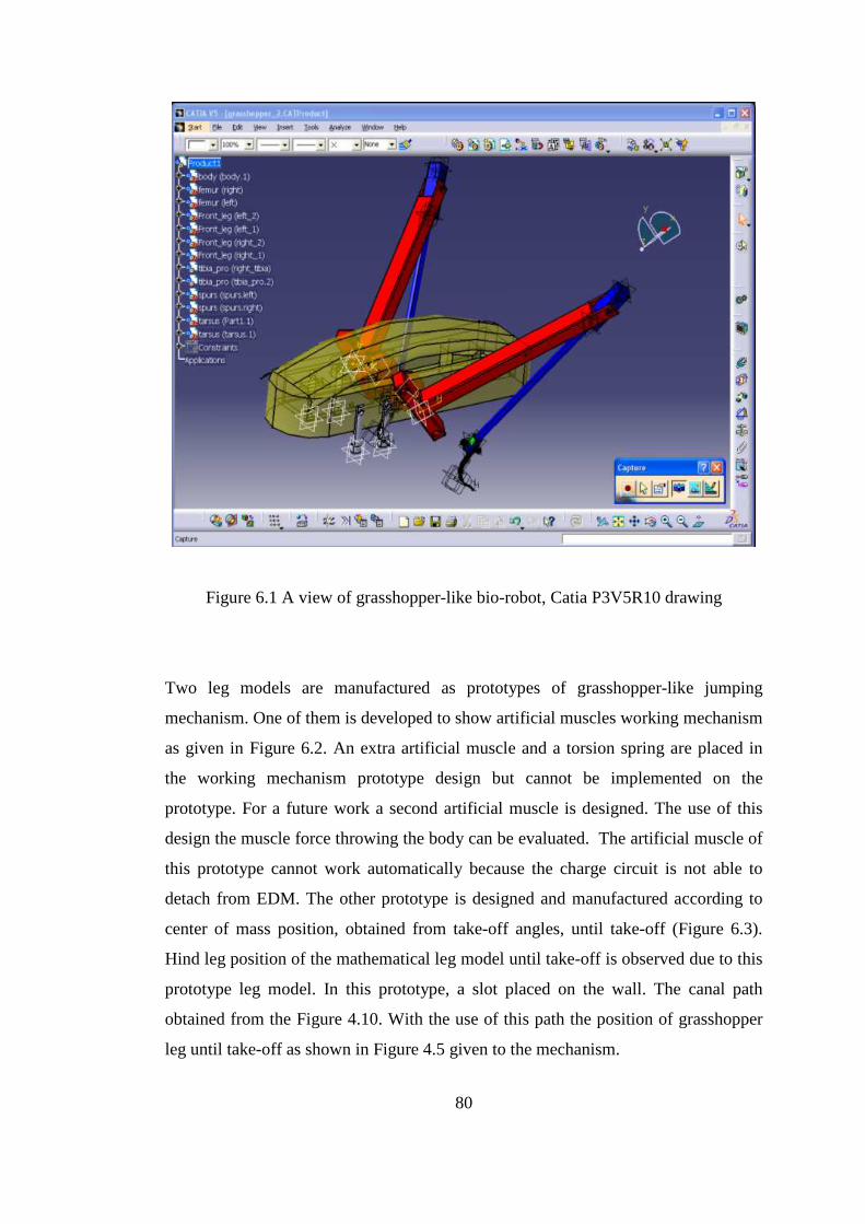
80
Figure 6.1 A view of grasshopper-like bio-robot, Catia P3V5R10 drawing
Two leg models are manufactured as prototypes of grasshopper-like jumping
mechanism. One of them is developed to show artificial muscles working mechanism
as given in Figure 6.2. An extra artificial muscle and a torsion spring are placed in
the working mechanism prototype design but cannot be implemented on the
prototype. For a future work a second artificial muscle is designed. The use of this
design the muscle force throwing the body can be evaluated. The artificial muscle of
this prototype cannot work automatically because the charge circuit is not able to
detach from EDM. The other prototype is designed and manufactured according to
center of mass position, obtained from take-off angles, until take-off (Figure 6.3).
Hind leg position of the mathematical leg model until take-off is observed due to this
prototype leg model. In this prototype, a slot placed on the wall. The canal path
obtained from the Figure 4.10. With the use of this path the position of grasshopper
leg until take-off as shown in Figure 4.5 given to the mechanism.

81
a. b.
Figure 6.2 a. A view of prototype design of leg model, Catia P3V5R10, b. The working mechanism of new artificial muscle prototype in a jumping leg model
(Atılım University, Biomimetic Design Laboratory)
Figure 6.3 Position of center of mass prototype in a jumping leg model until take-off (Atılım University, Biomimetic Design Laboratory)
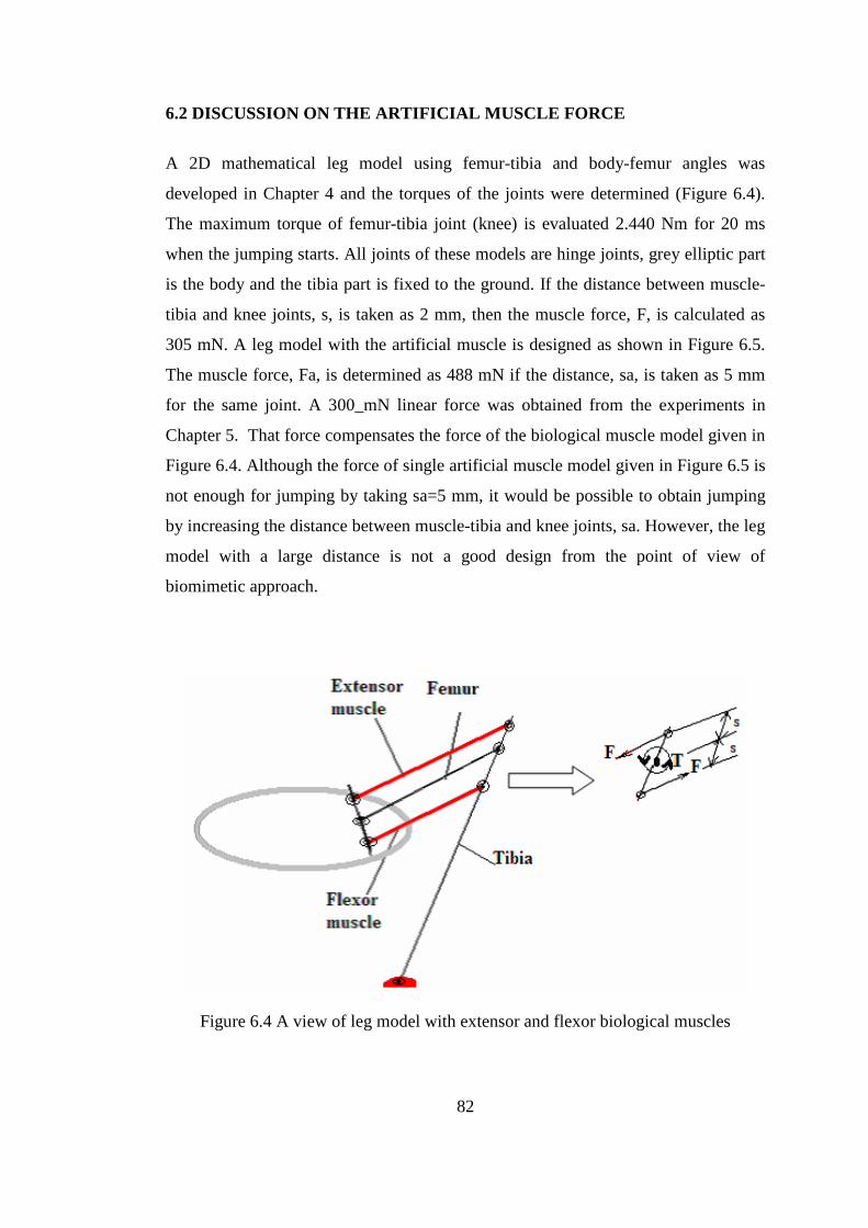
82
6.2 DISCUSSION ON THE ARTIFICIAL MUSCLE FORCE
A 2D mathematical leg model using femur-tibia and body-femur angles was
developed in Chapter 4 and the torques of the joints were determined (Figure 6.4).
The maximum torque of femur-tibia joint (knee) is evaluated 2.440 Nm for 20 ms
when the jumping starts. All joints of these models are hinge joints, grey elliptic part
is the body and the tibia part is fixed to the ground. If the distance between muscle-
tibia and knee joints, s, is taken as 2 mm, then the muscle force, F, is calculated as
305 mN. A leg model with the artificial muscle is designed as shown in Figure 6.5.
The muscle force, Fa, is determined as 488 mN if the distance, sa, is taken as 5 mm
for the same joint. A 300_mN linear force was obtained from the experiments in
Chapter 5. That force compensates the force of the biological muscle model given in
Figure 6.4. Although the force of single artificial muscle model given in Figure 6.5 is
not enough for jumping by taking sa=5 mm, it would be possible to obtain jumping
by increasing the distance between muscle-tibia and knee joints, sa. However, the leg
model with a large distance is not a good design from the point of view of
biomimetic approach.
Figure 6.4 A view of leg model with extensor and flexor biological muscles

83
Figure 6.5 A view of leg model using single artificial muscle
In this chapter, a pre-design of grasshopper-like bio-robot is evaluated using both
mathematical model and literature survey on grasshoppers. Although artificial
muscles designed to be placed on the femur in this model, the muscles are not
implemented. This design may be simulated and dynamic analysis can be evaluated
in MSC. Adams program to obtain torque and force data, these data would be
utilized to compare with mathematical and biological models.
Two prototypes for leg models are also manufactured to observe working mechanism
of the artificial muscle and position of centre of mass. Three segments, femur, tibia
and tarsus, are included in the prototypes. One of prototypes represents the position
of centre of mass and hind leg using a canal on the wall (Figure 6.3). The other one is
produced to show the artificial muscle working mechanism. However, the muscle
cannot work automatically, because the lack of charge circuit apart from the EDM.

84
CHAPTER 7
CONCLUSIONS AND FURTHER RECOMMENDATIONS
As the conclusion of this thesis, discussion of the whole work is presented and the
suggestions for future work are given.
7.1 DISCUSSION AND CONCLUSIONS
The aim of this thesis is to design a grasshopper-like jumping mechanism using
biomimetic design approach. Constraints on the design of grasshopper-like jumping
mechanism are specified in this study. A literature survey is conducted on the
anatomy of jumping mechanism of grasshoppers. In addition, an apteral type of
grasshoppers, Isophya nervosa, is studied as a biological observation part of the
biomimetic design. Because of the lack of special set-ups to observe the motion of
insects, the study on the anatomy is limited with the literature survey.
Since biomimetic study has become widespread, more universities worked on bio-
robots which are mimicked insects or other animals intensively. Literature survey on
bio-robots is evaluated while the mathematical model of the jumping leg mechanism
is studied. All mathematical solution is compared with different methods. The
position of the centre of mass of the body and the torque of hip and knee joints are
developed using 2D and 3D leg models. The constructed mathematical model is used
for production of prototypes and design of a new artificial muscle.
An electrical discharge system is used to have a light and small actuator. An
explosion due to electric discharge between two electrodes constructed in a piston-
cylinder system is used as an actuator. The cylinder is filled with dielectric liquid as
a fuel because of the low cost and environmental aspects. With this system, a new

85
artificial muscle is developed as an actuator for jumping mechanism of grasshopper-
like bio-robot in the thesis though there are several alternative artificial muscles
which have constraints with their size and application areas.
A piston-cylinder system with 4.78 mm outer and 3.78 mm inner diameter filled with
25.7 mm dielectric liquid height can give 300 mN on the average. The weight of the
designed piston-cylinder system is about 0.8 gr giving a force to weight ratio of the
artificial muscle developed about 38:1. That ratio is smaller than the ratio for
pneumatic artificial muscles but it is larger than the ratio for electrical motors and
pneumatic cylinders. The artificial muscle percentage elongation is expected to be
higher compared to that of natural muscles and the other artificial muscles due to
explosion in the cylinder and that percentage gives higher than SMAs and
piezoelectric artificial muscles, but that is not close to natural muscles. The muscle
reaction speed is fast giving reaction in msec, which would be comparable with that
of natural muscles and the other artificial muscles.
The measured force of the new artificial muscle is compared with the force obtained
from the mathematical leg model. The average experimental force of the artificial
muscle is close to that of mathematical leg model. However, the force obtained from
the leg design which is driven by an artificial muscle, cannot give necessary jumping
force. An extra artificial muscle implementation to the system is necessary to supply
jumping mechanism as a future study.
Two prototypes are developed to verify the mathematical and artificial muscle
models while a grasshopper-like bio-robot is designed. One of the prototypes is used
to represent the working mechanism of artificial muscle and the other shows the path
of the body centre of mass of grasshopper until take-off. Legs positions and body-
femur, femur-tibia and tibia-ground angles can be observed by using the prototype. If
the production of an electrical circuit separates from EDM, the prototypes can be
worked with artificial muscles.

86
As conclusion;
- By applying electric voltage to the electrodes with a small gap in a piston-
cylinder arrangement filled with a dielectric fluid, it is shown that it is
possible to get an explosion which gives force for the actuation of leg
mechanism for jumping.
- For a 3.78-mm piston-cylinder diameter and a 25.7-mm fluid height, for 235
V applied, a 300 mN force on the average can be obtained.
- For the designed muscle, a force to weight ratio of 38:1 can be obtained
- An extra artificial muscle or more powerful muscle implementation to the
system is necessary to supply jumping mechanism of the grasshopper with
500 mgr weight.
- If the production of an electrical circuit is separated from EDM, the leg
model of the prototypes can be worked with the artificial muscles.
7.2 SUGGESTIONS FOR FUTURE WORK
- In the mathematical model, one of the femur-tibia angles, )(tγ , is set constant
at 30°. Although the angle has a small change during lift-off and the effect of
that angle may be added in mathematical model as a future study.
- MSC. Adams program is used with a simple spherical model for determining
the horizontal distance, kinetic energy, etc. This simulation program can be
utilized for analyzing kinematics of the grasshopper-like bio-robot design,
given in Chapter 5.
The linear motion of artificial muscle has been accomplished but further
development of its performance can be improved. Those can be listed as follows:
- The piston-cylinder mechanism must be a closed system. If this closed
system can be constructed, the discharge and vaporization effects will
increase. The feed motion gap of the movable electrode on the cylinder
causes vapor to escape which must push the piston. However, the closed

87
system prevents the feed motion of electrodes because the feed motion gap is
closed; discharge features in a closed system may be obstructed.
- Because of the fact that EDM has still driven the discharge process, the force
capacity of the developed muscle is limited. A more powerful power supply
is to be used and RC circuit should be improved by a large size capacitor.
- The artificial muscle is not a soft actuator; this system may be moved in a soft
tube as a future work, so it becomes softer tissue like the natural muscle.

88
REFERENCES
1. Arora, S., 2005, “Development of dielectric elastomer based prototype fiber
actuators”, Thesis, North Carolina State University
http://www.lib.ncsu.edu/theses/available/etd-07282005-
145223/unrestricted/etd.pdf
(Download Date: 26.12.2006)
2. Ashley, 2003, “Artificial Muscles”, Scientific American, www.sciam.com
(Download Date: 04.07.2006)
3. Bar-Cohen, Y., 1997, “Low Mass Muscle Actuators (LoMMAs)”,
http://ndeaa.jpl.nasa.gov/nasa-nde/lommas/lommas97.pdf
(Download date: 30.06.2006)
4. Bar-Cohen, Y., Xue, T., Joffe, B., Lif, S. S., Shahinpoor, M., Simpson, J., Smith,
J., and Willis, P., 1997, “Electroactive Polymers (EAP) Low Mass Muscle
Actuators”, Proceedings of SPIE--Volume 3041, Smart Structures and Materials
1997: Smart Structures and Integrated Systems, Mark E. Regelbrugge, Editor,
June 1997, pp. 697-701
5. Bar-Cohen, Y., Leary, S., Yavrouian, A., Oguro, K., Tadokoro, S., Harrison, J.,
Smith, J., and Su, J., 1999, “Challenges to the Transition of IPMC Artificial
Muscle Actuators to Practical Application”, MRS Symposium: FF: Electroactive
Polymers, Nov. 29 to Dec. 1, 1999 at Boston, MS Document ID: 31295.
6. Bar-Cohen, Y., 2000, “Electroactıve polymers as artificial muscles -capabilities,
potentials and challenges”, Handbook on Biomimetics, Yoshihito Osada (Chief
Ed.), Section 11, in Chapter 8, “Motion” paper #134, publisher: NTS Inc., Aug.
2000

89
7. Bar-Cohen, Y., 2004, “Electroactive Polymers (EAP) as actuators for potential
future planetary mechanisms”, Proceedings of the 2004 NASA/DoD Conference
on Evolution Hardware (EH’04).
8. Bar-Cohen, Y., 2005, “Electroactive Polymers as Artificial Muscles Reality,
Potential and Challenges”, SPIE EAPAD-Short Course, March 6, San Diego,
California.
9. Bar-Cohen, Y., 2006, “Biomimetics-using nature to inspire human innovation”,
Bioinsp. Biomim. 1, P1-P12.
10. Başaran, D., 2003, “Design, Production and development of mini/micro robots to
form a cooperative colony”, Middle east Technical University, Department of
Mechanical Engineering Master Thesis, pg 98
11. Bennet-Clark, H.C., 1975, “The energetics of the jump of the locust Schistocerca
gregaria”, J. Exp. Biol., 63, 53-83
12. Biomimetic, 2006, “Abstract”
http://www-cdr.stanford.edu/biomimetics/pdf/biomimetics.pdf
(Download Date: 27.06.2006)
13. Biorobotics, 2006, “Biorobotics - Build Your Own Robotic Air Muscle Actuator”
http://www.imagesco.com/articles/airmuscle/AirMuscleDescription01.html
(Download date: 27.06.2006)
14. Birch, M.C., Quinn, R.D., Hahm, G., Phillips, S.M., Drennan, B., Fife, A., Beer,
R.D. and Hiten, V., 2000, “Design of a Cricket Microrobot”, Proceedings of the
2000 IEEE International Conference on Robotics and Automation (ICRA’00),
San Francisco, CA

90
15. Birch, M.C., Quinn, R.D., Hahm, G., Phillips, S.M., Drennan, B., Fife, A., Beer,
R.D.,Yu, X., Garverick, S:L., Laksanacharoen, S., Pollack, A.J. and Ritzmann,
R.E., 2005, “A Miniature Hybrid Robot Propelled by Legs”, Case Western
University,
16. Bonser,R.H.C., Harwin, W.S., Hayes, W., Jeronimidis, G., Mitchell, G.R., and
Santulli, C., 2004, “EAP-based artificial muscles as an alternative to space
mechanisms”
http://ndeaa.jpl.nasa.gov/ndeaa-pub/Japan/biomimetic-polymers-handbook.pdf
(Download Date: 25.07.2006)
17. Brabham, K., Marr, M., Smith, A., and Lee, P., 2004, “Artificial Muscle”,
http://web.cecs.pdx.edu/~mperkows/CLASS_ROBOTICS/FEBR26-
2004/ArtificialMusclePresentation.ppt#1
(Download date: 18.10.2006)
18. Brown,C., 2004, “Getting a grip on artificial muscles”,
http://www.eetimes.com/showArticle.jhtml?articleID=49400133
(Download date: 04.07.2006)
19. Burrows, M. and Morris, G., 2001, “The Kinematics and Neural Control of high
speed kicking movements in the locust”, J. Exp. Biol., 204:3471-3481.
20. Burrows, M. and Morris, O., 2002, “Jumping in a winged stick insect”, J. Exp.
Biol., 206:1035-49.
21. Burrows, M. and Morris, O., 2003, “Jumping and kicking in bush crickets”, J.
Exp. Biol, 205:2399-412.

91
22. Caldwell, D.G., Medrano-Cerda, G.A., and Goodwin, M., 1994, “Characteristics
and Adaptive Control of Pneumatic Muscle Actuators for a Robotic Elbow”,
IEEE
23. Choi, H. R., Jung, K., Ryew, S., Nam, J., Jeon, J., Koo, J. C., and Tanie, K.,
2005, “Biomimetic soft actuator: design, modeling, control, and applications”,
IEEE/ASME Transactions on Mechatronics, vol. 10, no. 5, October 2005
24. Colbrunn, R.W., 2000, “Design and control of a robotic leg with braided
pneumatic actuators”, Case Western Reverse University, Department of
Mechanical and Aerospace Engineering Master Thesis
25. Delcomyn, F., and Nelson, M.E., 2000, “Architectures for a biomimetic hexapod
robot”, Robotics and Autonomous Systems 30 (2000) 5–15
26. Ducheon, C., 2005, “Robots will be of service with muscles, not motors”,
Industrial Robot: An International Journal 32/6 452-455
27. Elliott,C. J. H., Zumstein, N., Forman, O., Nongthomba, U. and Sparrow, J.C.,
2004, “Distance and force production during jumping in wild-type and mutant
Drosophila melanogaster”, J. Exp.Biol., 207: 3515-3522
28. Emporia State University, 2005,” A grasshopper jumping”,
http://www.emporia.edu/egps/tales/grasshoppers2.htm
(Download Date: 27.07.2005)
29. Enchanted Learning, 1999, Enchanted Learning, (1999), “Grasshopper”,
http://www.enchantedlearning.com/subjects/insects/orthoptera/Grasshopperprintout.
html
(Download Date: 13.07.2005)

92
30. Espenscheid, K.S., Quinn, R.D., Beer, R.D. and Chiel, H.J., 1993 “Leg
coordination mechanisms in the stick insect applied to hexapod robot
locomotion”, The Massachusetts Institute of Technology, Adaptive
Behavior, Vol.1,No.4:455-468
31. Fauske, G. M., 2002, “Anatomy of a Grasshopper”,
http://www.ndsu.nodak.edu/entomology/hopper/anatomy.htm
(Download Date: 13.07.2005)
32. Festo, 2006, “Fluidic Muscles; DMSP-../ MAS-..”, Operating instructions.
33. Granosik, G., and Borenstein, J., 2004, “Minimizing Air Consumption of
Pneumatic Actuators in Mobile Robots”, IEEE International Conference on
Robotics and Automation, New Orleans, LA., April 26-May 1, pp. 3634-3639.
34. Halloran, A.O., and Malley, F.O., 2004, “Materials and technologies for artificial
muscle: a review for the mechatronic muscle project”, P.J. Prendergast and P.E.
McHugh (Eds.), Topics in Bio-Mechanical Engineering, pp. 184-215.
35. Heitler, W.J., 2005, “How grasshoppers jump”,
http://www.st-andrews.ac.uk/~wjh/jumping/index.html
(Download Date: 01.07.2005)
36. Huge Herr, D. Robert G., 2004, “A Swimming Robot Actuated by Living Muscle
Tissue”, Journal of NeuroEngineering and Rehabilitation, October 28
37. Kapps, M., 2007, “Smart-Material Mechanisms as Actuation Alternatives for
Aerospace Robotics and Automation”,
http://isdc2.xisp.net/~kmiller/isdc_archive/fileDownload.php/?link=fileSelect&file
_id=295
(Download date: 25.07.2006)

93
38. Kerscher, T., Albiez, J., and Berns, K., 2002, “Joint control of the Six-Legged
Robot AirBug Driven by Fluidic Muscles”, Third International Workshop on
Robot Motion and Control, November 9-11.
39. Kikuchi, F., Ota, Y., and Hirose, S., 2003, “Basic Performance Experiments for
Jumping Quadruped”, Pmceedings of the 2003 IEEERSJ InU Conference on
Intelligent Robots and Systems Las Vegas. Nevada October
40. Kinglesley, D.A., 2005, “A Cockroach Inspired Robot with Artificial Muscles”,
Case Western Reserve University, Department of Mechanical and Aerospace
Engineering Thesis
41. Kistler data sheet, 2005, “Low Level Force Sensor”, Instruction Manual.
42. Konez, A., Erden, A., and Akkök, M., 2006, “Preliminary Design Analysis of
Like-grasshopper Jumping Mechanism”, The 12th International Conference on
Machine Design and Production, Volume II, pg. 829, September, Kuşadası,
Turkey
43. Kornbluh, R., Pelrine, R., Eckerle, J., Joseph J., 1998, “Electrostrictive polymer
artificial muscle actuators”, Proceedings of the 1998 IEEE International
Conference on Robotics & Automation Leuven, Belgium, May
44. Kumar, A., 2000, “Biosensors Based on Piezoelectric Crystal Detectors: Theory
and Application”, The Minerals, Metals & Materials Society,
http://www.tms.org/pubs/journals/JOM/0010/Kumar/Kumar-0010.html
(Download date: 25.07.2007)

94
45. Kuratle R. H. and Signer, A., “The Basic of Piezoelectric Measurement
Technology”,
http://www.kistler.com/medias/izS408kP5EZxP85D8YwBEd-30.pdf
(Download date: 25.07.2007)
46. Lambrecht, B.G. A., Horchler, A.D., and Quinn R.D., 2005, “A Small, Insect-
Inspired Robot that Runs and Jumps”, Proceedings of the 2005 IEEE
International Conference on Robotics and Automation Barcelona, Spain, April
2005
47. Laksanacharoen, S., Pollack, A. J., Nelson, G. M., Quinn, R. D. and Ritzmann, R. E.,
2005, “Biomechanics and simulation of cricket for Microrobot design”, Case Western
Reverse University
48. Lee, Y.K., Shimoyama, I., 2002, “A Multi-Channel Micro Valve for Micro
Pneumatic Artificial Muscle”, IEEE.
49. Leeuwen, M.V. and Vreeken, J., 2004, “A philosophy of minimalist biomimetic
robotics”,
http://www.karlaspelund.com/biomimes/biomime_links.htm
(Download Date: 22.07.2005)
50. Lowe, M., 2006, “Elastomers: Powerful Polymer”,
http://www.appliancedesign.com/CDA/Articles/Feature_Article/4adb4f336188b0
10VgnVCM100000f932a8c0____
(Download date: 27.10.2006)
51. Lynch, K. M., Peshkin, M. A., Eren, H., Elbestawi, M. A., Garshelis, I. J., Thorn,
R., Norris, P. M., Hosticka, B., Figueroa, J. F., Everett, H. R. (Bart), Ipson, S.S.,
and Liu, C., 2002, “Mechatronics Handbook”, Chapter 19, Sensors, CRC Press
LLC

95
52. Merali, Z., 2006, “Methanol-powered artificial muscles start to flex”,
http://www.newscientist.com/article.ns?id=dn8859
(Download date: 30.06.2006)
53. Morrey, J.M., Lambrecht, B., Horchler, A.D., Ritzmann, R.E., and Quinn, R.D.,
2003, “Highly Mobile and Robust Small Quadruped Robots”, Proceedings of the
2003 IEEURSJ Intl. Conference on Intelligent Robots and Systems Las Vegas,
Nevada October 2003
54. O’Halloran, A. and O’Malley, F., 2004, “Materials and Technologies For
Artificial Muscle: A Review For The Mechatronic Muscle Project”, P.J:
Prendergast and P.E. McHugh (Eds.), Topics in Bio-Mechanical Engineering, pp.
184-215
55. Pelrine, R., Kornbluh, R., Pei, Q., Stanford, S., Oh, S., Eckerle, J., Full, R.,
Rosenthal, M., and Meijer, K., 2002, “Dielectric Elastomer Artificial Muscle
Actuators: Toward Biomimetic Motion”, Smart Structures and Materials 2002:
Electroactive Polymer Actuators and Devices (EAPAD), 126 Yoseph Bar-Cohen,
Editor, Proceedings of SPIE Vol. 4695
56. Pfadt, R. E., 2002, “Field Guide to Common Western Grasshoppers”, Wyoming
Agricultural Experiment Station, Bulletin 912, Third Edition
57. Prnewswire, 2006, “Artificial Muscle Introduces World's First Line of Standard
Electroactive Polymer (EAP) Linear Actuators”,
http://www.prnewswire.com/cgi-bin/stories.pl?ACCT=104&STORY
=/www/story/01-25-2006/0004267359&EDATE=
(Download date: 27.06.2006)
58. Raibert, M.H., 1986 “Legged Robots That Balance”, MIT Press: Cambridge,
Massachusetts.

96
59. Raibert, M.H., 1993, “Legged Robots”, Biological Neural Networks in
Invertebrate Neuroethology and Robotics. Academic Press, Inc: New York.
60. Ringrose, R., 1997, “Self Stabilizing Running”, Proceedings of the 1997 IEEE
International Conference on Robotics and Automation, Albeuquerque, NM.
61. Safak, K.K., Adams G.G., 2002, “Modeling and simulation of an artificial muscle
and its application to biomimetic robot posture control”, Robotics and
Autonomous Systems 41 (2002) 225–243
62. Savant, A., 2003, “Leg design of walking robots”, Fr. C. Rodrigues Mstitute of
Technology, Mumbai University, Mechanical Engineering Department, Bs
Report
63. Shahinpoor, M., and Kim, K. J., 2004, “Ionic polymer–metal composites: IV.
Industrial and medical applications”, Smart Mater. Struct. 14, 197–214
64. Stanford, 2005, “Biomimetic Robots“, http://www-cdr.stanford.edu/biomimetics/
(Download date: 13.06.2006)
65. Stilson T., 1996, “Piezoelectric Sensors”,
http://soundlab.cs.princeton.edu/learning/tutorials/sensors/node7.html
(Download date: 25.07.2007)
66. Titech, 2006, “Jumping Quadruped driven by pneumatic power "AirHopper"”
http://www-robot.mes.titech.ac.jp/robot/walking/airhopper/airhopper_e.html
(Download date: 20.04.2007)
67. University of Reading, 1992, “The Centre for Biomimetics Brochure”
http://www.rdg.ac.uk/Biomim/home.htm
(Download date: 10.06.2006)
97
68. Virtualskies, 2007, “Shape-Memory Alloys”,
http://virtualskies.arc.nasa.gov/research/youDecide/shapeMemAlloys.html
(Download date: 27.06.2007)
69. Webb,B. and Harrison,R.R., 2005, “Integrating sensorimotor systems in a robot
model of cricket behavior”,
http://www.stir.ac.uk/staff/psychology/bhw1/phonotaxis/spie.pdf
(Download Date: 26.07.2005)
70. Wei, T.E., Nelson, G.M., Quinn, R.D., Verma, H. and Garverick, S.L., 2005,
“Design of a 5-cm Monopod Hopping Robot”, Case Western Reverse University

98
APPENDICES

99
APPENDIX A
ANALYTICAL SOLUTION OF BODY HEIGHT AND BODY-
FEMUR ANGLE
A. 1. Calculation of Body Height
If the body height and femur-tibia angle changes are assumed to be zero between the
time -80 ms and -20 ms in the Figure 4.2 in Chapter 4, the body height (according to
body centre of mass position) (z(t)) can be represented analytically by using the
empirical data obtained from the Figure A.1. Moreover, -20ms is shifted to origin for
positive time interval. It is assumed that body height (z(t)) polynomial is third
degree.
Figure A.1 Body height (z(t)) of body movement of a Pholidoptera male before take-off for positive time definite

100
According to this figure initial conditions are;
t=0 ms z(t)=5 mm (A.1)
t=5 ms z(t)=5.667 mm (A.2)
t=10 ms z(t)=7mm (A.3)
t=20 ms z(t)=10.667 mm (A.4)
A.1.1 Polynomial Solution
If body height (z(t)) polynomial is assumed to be third degree, it is represented with
dctbtattz +++= 23)( (A.5)
If the first initial condition is substituting into the equation of A.5, it is gotten,
t=0 ms z(t)=5 mm d=5 (A.6)
Substituting (A.6) into the (A.2)
bac 25125667.05 −−= (A.7)
Similarly, substituting (A.6) and (A.7) into the conditions (A.3) and (A.4), it is
gotten,
ba 50750666.0 += (A.8)
ba 3007500999.2 += (A.9)

101
Consequently, body height becomes
505018333.0018305.000332333.0)( 23 +++−= ttttz (A.10)
A.1.2 Lagrange Interpolating Polynomials Solution
∑=
=n
iiin xfxLxf
0
)().()( (A.11)
ijxx
xxxL
ji
jn
ji ≠
−−
∏==
,)(
)()(
0 (A.12)
For third order polynomial and interval of time, the formulation is
)().()().()().()().()().()( 33221100
3
03 tztLtztLtztLtztLtftLtz
iii +++==∑
=
(A.13)
Thus, body height is
667.5*)205)(105)(05(
)20)(10)(0(5*
)200)(100)(50(
)20)(10)(5()(3 −−−
−−−+−−−
−−−= tttttttz
7*)2010)(510)(010(
)20)(5)(0(
−−−−−−+ ttt
667.10*)1020)(520)(020(
)10)(5)(0(
−−−−−−+ ttt (A.14)
From the equation (A.14), body height becomes
50501833.001830501.000332334.0)( 23 +++−= ttttz (A.15)
A.1.3 Least Square Regression, Polynomial Regression Solution
012
23
3)( atatatatz +++= (A.16)
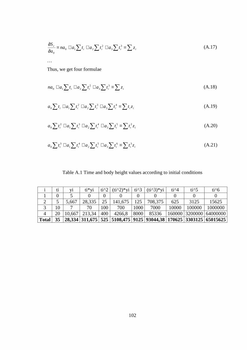
102
∑ ∑ ∑∑ =+++=∂∂
iiiir ztatatana
a
S 33
2210
0
(A.17)
…
Thus, we get four formulae
∑ ∑ ∑∑ =+++ iiii ztatatana 33
2210 (A.18)
∑ ∑ ∑∑∑ =+++ iiiiii zttatatata 43
32
210 (A.19)
∑ ∑ ∑∑∑ =+++ iiiiii zttatatata 253
42
31
20 (A.20)
∑ ∑ ∑ ∑ ∑=+++ iiiiii zttatatata 363
52
41
30 (A.21)
Table A.1 Time and body height values according to initial conditions
i ti yi ti*yi ti^2 (ti^2)*yi ti^3 (ti^3)*yi ti^4 ti^5 ti^6 1 0 5 0 0 0 0 0 0 0 0 2 5 5,667 28,335 25 141,675 125 708,375 625 3125 15625 3 10 7 70 100 700 1000 7000 10000 100000 1000000 4 20 10,667 213,34 400 4266,8 8000 85336 160000 3200000 64000000
Total 35 28,334 311,675 525 5108,475 9125 93044,38 170625 3303125 65015625

103
Mathcad 2000 Solution is given.
%Least square Regression, polynomial regression
V
28.334
311.675
5108.475
93044.38
:=M
4
35
525
9125
35
525
9125
170625
525
9125
170625
3303125
9125
170625
3303125
65015625
:=
soln lsolve M V,( ):=
soln
4.999995
0.0501942222
0.01830325
0.0003322722−
=
Body height becomes
z3 t( ) 0.0003322722−( ) t3⋅ 0.01830325( ) t2⋅+ 0.0501942222( ) t⋅+ 4.999995( )+:= (A.22)
A.1.4 Result of the Body Height Analysis
The graph of the body height according to difference analytical and numerical
solutions is given in the given Figure 4.11.
i. Polynomial Solution;
5)0501833.0()01830501.0()000332334.0()( 231 +++−= ttttz (4.23)

104
ii. Lagrange Interpolating Polynomilas Solution;
5)05018333.0()018305.0()000332333.0()( 232 +++−= ttttz (4.24)
iii. Least Square Regression Solution;
)999995.4()0501942222.0()01830325.0()0003322722.0()( 233 +++−= ttttz (4.25)
Figure A.2 Mathcad 2000 body height solutions, polynomial, Lagrange and least
square methods solutions
A. 2. Calculation of Femur-Tibia (Knee) Angle
If the body height and femur-tibia angle changes are assumed to be zero between the
time -80 ms and -20 ms in the Figure 4.2 in Chapter 4, the Femur-Tibia angle ( )(tα )
can be represented analytically by using the empirical data obtained from the Figure

105
A.2. Moreover, -20ms is shifted to origin for positive time interval. It is assumed that
the Femur-Tibia angle ( )(tα ) polynomial is third degree like body height
polynomial.
Figure A.3 Femur-Tibia angle ( )(tα ) of body movement of a Pholidoptera male before take-off for positive time definite
According to this figure initial conditions are;
t=0 ms )(tα =20 deg (A.23)
t=5 ms )(tα =28 deg (A.24)
t=10 ms )(tα =50 deg (A.25)
t=20 ms )(tα =140 deg (A.26)

106
A.2.1 Polynomial Solution
If Femur-Tibia angle ( )(tα ) polynomial is third degree, it is represented with
hgtftett +++= 23)(α (A.27)
If similar way with body height is used, femur-tibia angle becomes
2026666675.026.000133333.0)( 23 +++= ttttα (A.28)
A.2.2 Lagrange Interpolating Polynomials
For third order polynomial and interval of time, the formulation of Femur-tibia angle
is
)().()().()().()().()().()( 33221100
3
03 ttLttLttLttLttLt
iii αααααα +++==∑
=
(A.29)
Thus, femur-tibia angle is
28*)205)(105)(05(
)20)(10)(0(20*
)200)(100)(50(
)20)(10)(5()(3 −−−
−−−+−−−
−−−= tttttttα
50*)2010)(510)(010(
)20)(5)(0(
−−−−−− ttt
140*)1020)(520)(020(
)10)(5)(0(
−−−−−−+ ttt (A.30)
From the equation (8), angle polynomial becomes
202666669.025999994.0001333337.0)( 23 +++= ttttα (A.31)
A.2.3 Least Square Regression, Polynomial Regression
012
23
3)( atatatat +++=α (A.32)

107
Thus, we get four formulae
∑ ∑ ∑∑ =+++ iiii tatatana α33
2210 (A.33)
∑ ∑ ∑∑∑ =+++ iiiiii ttatatata α43
32
210 (A.34)
∑ ∑ ∑∑∑ =+++ iiiiii ttatatata α253
42
31
20 (A.35)
∑ ∑ ∑ ∑ ∑=+++ iiiiii ttatatata α363
52
41
30 (A.36)
Table A.2 Time and the angle values according to initial conditions
i ti αi ti* αi ti^2 (ti^2)*αi ti^3 (ti^3)*αi ti^4 ti^5 ti^6 1 0 20 0 0 0 0 0 0 0 0 2 5 28 140 25 700 125 3500 625 3125 15625 3 10 50 500 100 5000 1000 50000 10000 100000 1000000 4 20 140 2800 400 56000 8000 1120000 160000 3200000 64000000
Total 35 238 3440 525 61700 9125 1173500 170625 3303125 65015625
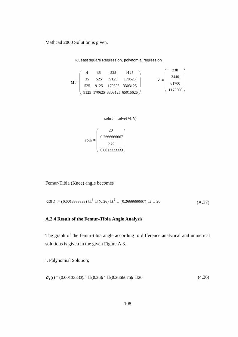
108
Mathcad 2000 Solution is given.
%Least square Regression, polynomial regression
V
238
3440
61700
1173500
:=M
4
35
525
9125
35
525
9125
170625
525
9125
170625
3303125
9125
170625
3303125
65015625
:=
soln lsolve M V,( ):=
soln
20
0.2666666667
0.26
0.0013333333
=
Femur-Tibia (Knee) angle becomes
α3 t( ) 0.0013333333( ) t3⋅ 0.26( ) t2⋅+ 0.2666666667( ) t⋅+ 20+:= (A.37)
A.2.4 Result of the Femur-Tibia Angle Analysis
The graph of the femur-tibia angle according to difference analytical and numerical
solutions is given in the given Figure A.3.
i. Polynomial Solution;
20)2666675.0()26.0()00133333.0()( 231 +++= ttttα (4.26)

109
ii. Lagrange Interpolating Polynomilas Solution;
20)2666669.0()25999994.0()001333337.0()( 232 +++= ttttα (4.27)
iii. Least Square Regression Solution;
20)2666666667.0()26.0()0013333333.0()( 233 +++= ttttα (4.28)
Figure A.4 Mathcad 2000 femur-tibia angle solutions, polynomial, Lagrange and
least square methods solutions
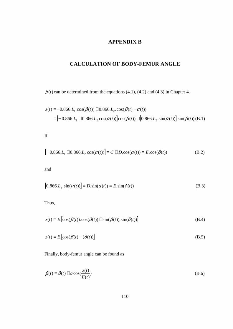
110
APPENDIX B
CALCULATION OF BODY-FEMUR ANGLE
)(tβ can be determined from the equations (4.1), (4.2) and (4.3) in Chapter 4.
))()(cos(..866.0))(cos(..866.0)( 21 ttLtLtz αββ −+−=
[ ] [ ] ))(sin(.))(sin(..866.0))(cos())(cos(.866.0.866.0 221 ttLttLL βαβα ++−= (B.1)
If
[ ] ))(cos(.))(cos(.))(cos(.866.0.866.0 21 tEtDCtLL δαα =+=+− (B.2)
and
[ ] ))(sin(.))(sin(.))(sin(..866.0 2 tEtDtL δαα == (B.3)
Thus,
[ ]))(sin()).(sin())(cos()).(cos(.)( ttttEtz δβδβ += (B.4)
[ ]))(()(cos(.)( ttEtz δβ −= (B.5)
Finally, body-femur angle can be found as
))(
)(cos()()(
tE
tzatt += δβ (B.6)

111
where ( ) 22 ))(sin(.())(cos(.)( tDtDCtE αα ++= ;
+=
))(cos(.
))(sin(.tan)(
tDC
tDat
ααδ ;
))(cos(.1 tLC γ−=
and
))(cos(.2 tLD γ=

112
APPENDIX C
2D LEG MODEL RESULTS
Table C.1 2D Leg Model Angles Results
time Alfa (deg)
Beta (deg)
Teta= Beta-alfa
(deg)
x(t) (mm)
z(t) (mm)
Velocity (mm/ms^2)
0.000 20,0 -55,2 -75,2 1.175 5.000 0.562 0.500 20,1 -57,6 -77,7 0.968 5.051 0.258 1.000 20,3 -57,7 -78 0.970 5.104 0.269 1.500 20,7 -55,5 -76,2 1.183 5.160 0.579 2.000 21,2 -52,3 -73,5 1.508 5.219 0.723 2.500 21,9 -48,7 -70,6 1.884 5.281 0.797 3.000 22,7 -45,1 -67,8 2.290 5.348 0.847 3.500 23,7 -41,5 -65,2 2.718 5.420 0.888 4.000 24,8 -38,0 -62,8 3.165 5.496 0.927 4.500 26,1 -34,7 -60,8 3.631 5.579 0.965 5.000 27,5 -31,5 -59 4.115 5.667 1.005 5.500 29,0 -28,4 -57,4 4.618 5.762 1.045 6.000 30,8 -25,4 -56,2 5.141 5.864 1.087 6.500 32,7 -22,6 -55,3 5.685 5.974 1.130 7.000 34,7 -19,8 -54,5 6.248 6.093 1.173 7.500 36,9 -17,2 -54,1 6.832 6.219 1.217 8.000 39,2 -14,6 -53,8 7.436 6.355 1.261 8.500 41,6 -12,1 -53,7 8.060 6.501 1.304 9.000 44,3 -9,7 -54 8.704 6.657 1.346 9.500 47,1 -7,3 -54,4 9.367 6.823 1.387 10.000 50,0 -5,0 -55 10.048 7.001 1.427 10.500 53,0 -2,7 -55,7 10.745 7.190 1.464 11.000 56,3 -0,4 -56,7 11.458 7.392 1.498 11.500 59,7 1,9 -57,8 12.184 7.606 1.529 12.000 63,2 4,1 -59,1 12.921 7.833 1.556 12.500 66,9 6,4 -60,5 13.667 8.074 1.579 13.000 70,7 8,6 -62,1 14.419 8.329 1.597 13.500 74,6 10,8 -63,8 15.174 8.599 1.609 14.000 78,8 13,1 -65,7 15.928 8.884 1.615 14.500 83,1 15,3 -67,8 16.678 9.185 1.615 15.000 87,5 17,5 -70 17.419 9.502 1.608 15.500 92,1 19,8 -72,3 18.147 9.835 1.593 16.000 96,8 22,0 -74,8 18.857 10.186 1.571 16.500 101,7 24,3 -77,4 19.542 10.554 1.541 17.000 106,7 26,6 -80,1 20.198 10.940 1.503 17.500 111,9 28,8 -83,1 20.817 11.345 1.457 18.000 117,2 31,1 -86,1 21.394 11.770 1.405 18.500 122,7 33,3 -89,4 21.919 12.213 1.347 19.000 128,3 35,6 -92,7 22.386 12.677 1.286 19.500 134,1 37,9 -96,2 22.785 13.162 1.227 20.000 140,0 40,1 -99,9 23.107 13.668 1.176

113
APPENDIX D
CALCULATION OF MASSES AND VOLUMES OF
FEMUR-TIBIA
To find the limb mass, models of the femur and tibia are given in the Figure D.1.
Masses of the femur and tibia:
Femur Tibia
D1 D2 D3
l1 l2 l3
Figure D.1 Mathematical models of the femur and tibia.
Where
l1= 10.26 mm; D1= 3.2 mm
l2= 6.84 mm; D2= 0.8 mm
l3= 15.6 mm; D3= 0.6 mm

114
Volume of the femur and tibia:
32
22
1
21 958.85.
4
..
4
.mml
Dl
DV femur =+= ππ
(D.1)
33
23 41.4.
4
.mml
DVtibia == π
(D.2)
)(10.107.88)()10.(958.85)./(025.1.1 93333 kgmmkgVM femur−− === ρ (D.3)
)(10.52.4)()10.(41.4)./(025.1.2 93333 kgmmkgVM tibia−− === ρ (D.4)

115
APPENDIX E
DYNAMIC MODEL OF THE GRASSHOPPER LEG
A Lagrange’s method is used for arriving at equations between joint power and foot
coordinates. For assumed mass distribution;
a. Kinetic Energy;
Kinetic Energy of M1 is;
)(2
1 21
2111 zxMK && += (E.1)
where
))(sin(..866.0))(sin(.2
.866.0 21
1 tLtL
x θβ −= (E.2)
))(cos(..866.0))(cos(.2
.866.0 21
1 tLtL
z θβ +−= (E.3)
and
)()).(cos(..866.0)()).(cos(..433.0 211 ttLttLx θθββ &&& −= (E.4)
)()).(sin(..866.0)()).(sin(..433.0 211 ttLttLz θθββ &&& −= (E.5)

116
Substituting these equations into the equation;
[ ])().()).()(cos(75.0)(75.0)(.188.02
121
222
22111 ttttLLtLtLMK θβθβθβ &&&& −−+= (E.6)
Kinetic Energy of M2 is;
2222
22
222 ...125.0))(90(.
2.
2
1 θθ &LMtdt
dLMK =
+
= (E.7)
Kinetic Energy of Mh is;
)(2
1 22hhhh zxMK && += (E.8)
where
))(sin(..866.0))(sin(..866.0 21 tLtLxh θβ −= (E.9)
))(cos(..866.0))(cos(..866.0 21 tLtLzh θβ +−= (E.10)
and
)()).(cos(..866.0)()).(cos(..866.0 21 ttLttLxh θθββ &&& −= (E.11)
)()).(sin(..866.0)()).(sin(..866.0 21 ttLttLzh θθββ &&& −= (E.12)
Substituting these equations into the equation;
[ ])().()).()(cos(5.1)(75.0)(.75.02
121
222
221 ttttLLtLtLMK hh θβθβθβ &&&& −−+= (E.13)
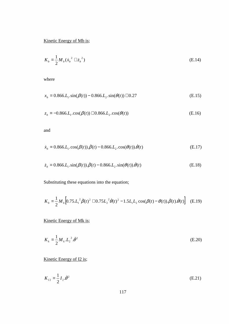
117
Kinetic Energy of Mb is;
)(2
1 22bbbb zxMK && += (E.14)
where
27.0))(sin(..866.0))(sin(..866.0 21 +−= tLtLxb θβ (E.15)
))(cos(..866.0))(cos(..866.0 21 tLtLzb θβ +−= (E.16)
and
)()).(cos(..866.0)()).(cos(..866.0 21 ttLttLxb θθββ &&& −= (E.17)
)()).(sin(..866.0)()).(sin(..866.0 21 ttLttLzb θθββ &&& −= (E.18)
Substituting these equations into the equation;
[ ])().()).()(cos(5.1)(75.0)(.75.02
121
222
221 ttttLLtLtLMK bb θβθβθβ &&&& −−+= (E.19)
Kinetic Energy of Mk is;
222 ..
2
1 θ&LMK kk = (E.20)
Kinetic Energy of I2 is;
222 .
2
1 θ&IK I = (E.21)

118
Kinetic Energy of I1 is;
211 .
2
1 β&IK I = (E.22)
Kinetic Energy of Ib is;
0=IbK (E.23)
b. Potential Energy;
−−−−= ))(cos(2
))(cos())(cos())(cos(2
1212
22 t
LtLgMtgLMt
LgMP k βθθθ
[ ] 212 ))()((
2
1))(cos())(cos()( ttktLtLgMM bh θββθ −+−+− (E.24)
Thus,
gtLMMMMMP bhk ))(cos()5.0( 212 θ++++−=
211 ))()((
2
1))(cos()5.0( ttkgtLMMM bh θββ −++++ (E.25)
c. Using Lagrange’s Method for Knee Actuator (Mk);
θθ ∂∂
−
∂∂
= aa LL
dt
dT
&2 (E.26)
θθθθθθθθθθ ∂∂−
∂∂+
∂∂+
∂∂
+∂
∂+
∂∂
+∂
∂+∂∂=−
∂∂=
∂∂ PKKKKKKK
PKL IIkbha 1221)( (E.27)
)().()).()(sin(375.0 2111 ttttLLM
K θβθβθ
&&−−=∂∂
(E.28)

119
0122 =∂
∂=∂
∂=∂
∂=
∂∂
θθθθIIk KKKK
(E.29)
)().()).()(sin(75.0 21 ttttLLMK
hh θβθβ
θ&&−−=
∂∂
(E.30)
)().()).()(sin(75.0 21 ttttLLMK
bb θβθβ
θ&&−−=
∂∂
(E.31)
))()(())(sin()5.0( 212 ttkgtLMMMMMP
bhk βθθθ
−+++++=∂∂
(E.32)
)().()).()(sin())(75.0375.0( 211 ttttLLMMML
bha θβθβ
θ&&−++−=
∂∂
))()(())(sin()5.0( 212 ttkgtLMMMMM bhk βθθ −+++++− (E.33)
θθθθθθθθθθ &&&&&&&&&& ∂∂−
∂∂+
∂∂+
∂∂
+∂
∂+
∂∂
+∂
∂+∂∂=−
∂∂=
∂∂ PKKKKKKK
PKL IIkbha 1221)( (E.34)
)())()(cos(375.0)(.75.0 2112
211 tttLLMtLM
K βθβθθ
&&&
−−=∂∂
(E.35)
)(.25.0 222
2 tLMK θθ
&&
=∂
∂ (E.36)
)())()(cos(75.0)(.75.0 212
2 tttLLMtLMK
hhh βθβθ
θ&&
&−−=
∂∂
(E.37)
)())()(cos(75.0)(.75.0 212
2 tttLLMtLMK
bbb βθβθ
θ&&
&−−=
∂∂
(E.38)
)(.22 tLM
Kk
k θθ
&&
=∂
∂ (E.39)

120
)(.22 tI
K I θθ
&&
=∂
∂ (E.40)
01 =∂∂=
∂∂
θθ &&
PK I (E.41)
)(.)(75.0 221 tLMMM
Lbh
a θθ
&&
++=∂∂
[ ] θβθβ && )()())()(cos()(75.0375.0 22
2211 ILMtttLLMMM kbh ++−++− (E.42)
[ ] )(.))(75.0( 22
21 tILMMMML
dt
dkbh
a θθ
&&&
++++=
∂∂
[ ] [ ])()).()(cos()())()())(()(sin()(75.0375.0 211 ttttttttLLMMM bh βθββθβθβ &&&&& −+−−−++−
(E.43)
Thus, torque becomes,
542
3212 ))(()()(. GgGtGtGtGT ++++= ββθ &&&&& (E.44)
where
22
211 ).)(75.0( ILMMMMG kbh ++++= (E.45)
))()(cos())(75.0375.0( 2112 ttLLMMMG bh θβ −++−= (E.46)
))()(sin())(75.0375.0( 2113 ttLLMMMG bh θβ −++= (E.47)
))(sin()5.0( 2124 tLMMMMMG bhk θ++++= (E.48)
))()((5 ttkG βθ −= (E.49)

121
d. Using Lagrange’s Method for Hip Actuator (Mh);
ββ ∂∂
−
∂∂
= aa LL
dt
dT
&1 (E.50)
ββββββββββ ∂∂−
∂∂
+∂
∂+
∂∂
+∂
∂+
∂∂
+∂
∂+
∂∂
=−∂∂=
∂∂ PKKKKKKK
PKL IIkbha 1221)( (E.51)
)().()).()(sin(375.0 2111 ttttLLM
K θβθββ
&&−−=∂∂
(E.52)
0122 =∂
∂=∂
∂=∂
∂=
∂∂
θθθθIIk KKKK
(E.53)
)().()).()(sin(75.0 21 ttttLLMK
hh θβθβ
θ&&−−=
∂∂
(E.54)
)().()).()(sin(75.0 21 ttttLLMK
bb θβθβ
θ&&−−=
∂∂
(E.55)
))()(())(sin()5.0( 11 ttkgtLMMMP
bh θββθ
−+++−=∂∂
(E.56)
)().()).()(sin())(75.0375.0( 211 ttttLLMMML
bha θβθβ
θ&&−++−=
∂∂
))()(())(sin()5.0( 11 ttkgtLMMM bh θββ −−+++ (E.57)
ββββββββββ &&&&&&&&&& ∂∂−
∂∂
+∂
∂+
∂∂
+∂
∂+
∂∂
+∂
∂+
∂∂
=−∂∂=
∂∂ PKKKKKKK
PKL IIkbha 1221)( (E.58)
)())()(cos(375.0)(.188.0 2112
111 tttLLMtLM
K θθββθ
&&&
−−=∂∂
(E.59)

122
022 =∂∂=
∂∂
=∂
∂=
∂∂
ββββ &&&&
PKKK Ik (E.60)
)())()(cos(75.0)(.75.0 212
1 tttLLMtLMK
hhh θθββ
β&&
&−−=
∂∂
(E.61)
)())()(cos(75.0)(.75.0 212
1 tttLLMtLMK
bbb θθββ
β&&
&−−=
∂∂
(E.62)
)(11 tI
K I ββ
&&
=∂
∂ (E.63)
)().))(75.0188.0( 12
11 tILMMML
bha β
β&
&+++=
∂∂
[ ] )())()(cos()(75.0375.0 211 tttLLMMM bh θθβ &−++− (E.64)
[ ] )(.))(75.0188.0( 12
11 tILMMML
dt
dbh
a ββ
&&&
+++=
∂∂
[ ] ( )[ ])()).()(cos())()()())(()(sin()(75.0375.02
211 ttttttttLLMMM bh θθβθθβθβ &&&&& −−−−+++(E.65)
Thus, torque becomes,
572
33621 ))(()()(2)()(. GgGtGttGtGtGT −+−++= θθββθ &&&&&&& (E.66)
where
12
116 ).)(75.0188.0( ILMMMMG kbh ++++= (E.67)
))(sin()5.0( 117 tLMMMG bh β++−= (E.68)
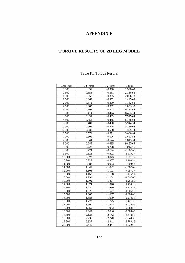
123
APPENDIX F
TORQUE RESULTS OF 2D LEG MODEL
Table F.1 Torque Results
Time (ms) T1 (Nm) T2 (Nm) T (Nm) 0.000 0.351 -0.350 1.590e-3 0.500 0.354 -0.351 2.130e-3 1.000 0.357 -0.355 2.086e-3 1.500 0.363 -0.362 1.445e-3 2.000 0.372 -0.370 1.152e-3 2.500 0.383 -0.382 1.021e-3 3.000 0.397 -0.397 9.282e-4 3.500 0.414 -0.414 8.432e-4 4.000 0.434 -0.433 7.597e-4 4.500 0.456 -0.455 6.768e-4 5.000 0.481 -0.480 5.944e-4 5.500 0.508 -0.508 5.126e-4 6.000 0.538 -0.538 4.309e-4 6.500 0.571 -0.571 3.490e-4 7.000 0.606 -0.606 2.662e-4 7.500 0.644 -0.644 1.817e-4 8.000 0.685 -0.685 9.457e-5 8.500 0.728 -0.728 4.012e-6 9.000 0.774 -0.774 -9.087e-5 9.500 0.822 -0.822 -1.910e-4 10.000 0.873 -0.873 -2.971e-4 10.500 0.926 -0.927 -4.100e-4 11.000 0.983 -0.983 -5.303e-4 11.500 1.041 -1.042 -6.587e-4 12.000 1.103 -1.103 -7.957e-4 12.500 1.167 -1.168 -9.416e-4 13.000 1.233 -1.234 -1.097e-3 13.500 1.302 -1.304 -1.261e-3 14.000 1.374 -1.376 -1.434e-3 14.500 1.449 -1.450 -1.616e-3 15.000 1.526 -1.527 -1.806e-3 15.500 1.605 -1.607 -2.005e-3 16.000 1.688 -1.690 -2.210e-3 16.500 1.772 -1.775 -2.421e-3 17.000 1.860 -1.863 -2.638e-3 17.500 1.950 -1.953 -2.860e-3 18.000 2.043 -2.046 -3.085e-3 18.500 2.138 -2.142 -3.313e-3 19.000 2.236 -2.240 -3.544e-3 19.500 2.337 -2.341 -3.780e-3 20.000 2.440 -2.444 -4.022e-3

124
APPENDIX G
ARTIFICIAL MUSCLES
Table G.1 Illustration the advantages and disadvantages of electronic and ionic EAPs as outlined by Halloran and Malley, 2004 and Bar-Cohen, 2004
EAP type Advantages Disadvantages
Electronic
- can operate in room conditions for a long time
- rapid response (msec levels) - can hold strain under dc
activation - induces relatively large
actuation forces
- requires high voltages (~150MV/m)
- requires compromise between strain and stress
- glass transition temperature is inadequate for low temperature actuation tasks and in the case of Ferroelectric EAP, high temperature applications are limited by the Curie temperature
- Mostly, producing a monopolar actuation independent of the voltage polarity due to associated electrostriction effect.
Ionic
- produces large bending displacements
- requires low voltage - natural bi-directional
actuation that depends on the voltage polarity
- except for CPs and NTs, ionic EAPs do not hold strain under dc voltage
- slow response (fraction of a second)
- bending EAPs induce a relatively low actuation force
- except for CPs, it is diffucult to produce a consistent material (particularly IPMC)
- In aqueous systems the material sustains electrolysis at voltages >1.23V
- To operate in air requires attention to the electrolyte
- Low electromechanical coupling efficiency

125
Table G.2 EAP infrastructure (Cohen, 2005)