DEVELOPING THE INDUCTIVE INDUCED POLARIZATION METHOD …

DEVELOPING THE INDUCTIVE INDUCED POLARIZATION

METHOD FOR THE DISCOVERY OF DISSEMINATED ORE

A proposal for the discovery of a new class of ore deposit with MultiLoop III

Spring 2011

Lamontagne Geophysics Ltd., 115 Grant Timmins Drive, Kingston, ON K7M 8N3 ◦ T: 613.531.9950 ◦ F: 613.531.8987# 1

DEVELOPING THE IIP METHOD

Justification

We seek to develop the interpretative capability to allow a new class of ore deposits to be more easily discovered - namely disseminated mineralization located in resistive crystalline rock. This class of mineralization has not been adequately targeted by conventional EM and IP exploration methods, as discussed below, and so provides the opportunity for new dis-coveries. Such deposits should be detectable with the Inductive Induced Polarization (IIP) method.

Deposits of disseminated mineralization situated in crystalline host rock could represent a major undiscovered resource. Such disseminated mineralization would appear as a weak conductor, and so could easily be overlooked by traditional EM exploration systems that are designed and optimized to target massive mineralization. Furthermore, because traditional induced polarization/ resistivity surveys rely on grounded sources, they would have difficulty energizing such mineralization: currents would likely to be channeled through fractures and conductive inhomogeneities and would be unlikely to energize the disseminated mineraliza-tion. Arguably, disseminated mineralization in crystalline rock is a resource waiting to be detected.

Inductive source energization is the better alternative for detecting disseminated minerali-zation in crystalline rock, but our knowledge of the method lacks the sophistication re-quired to target the mineralization and to reliably interpret the resulting IIP data. Accord-ingly, polarizable mineralization situated in resistive rock (for example brecchiated or dis-seminated sulphides, alteration minerals, conductive oxides such as cuprite, or mineraliza-tion associated with a polarizable accessory mineral such as hematite) could represent a new, under-explored category of mineral resource or mineral resource indicator.

Additionally, IIP responses, generally opposite in sign, may partially mask the response of a more-conductive core zone at late time. And IIP responses from surficial sources, such as lake-bottom sediments, can complicate or mask the response of late-time good conductors at depth. Understanding IIP can be of use in the search for highly-conductive, deep ore in which IIP could be a source of unwanted noise.

To better understand what the IIP method is capable of, and how to recognize IIP phe-nomena in EM data, we propose to develop modelling software to simulate IIP phenomena.


A simple model

To contrast the Inductive IP (IIP) method from the Galvanic (grounded source) IP (GIP) method, in which grounded current electrodes are used, consider the simple circuit dia-grams that represent each measurement. Each circuit contains a Drake model frequency

dependent impedance, Zd(ω), used to represent polarization phenomena with the frequency dependence pa-rameter B and static impedance Z. The series and parallel resistors, Rs and Rp, represent the ground resis-tance in series and in parallel with the polarization. The inductance of the circulating current in the ground ener-gized by the inductive source is repre-

sented by L.

As a simple illustration of IIP phenomena, consider the case of a polarizable thin plate energized by a step source of current shown in the inset figure. As the cur-rent is switched on, current is induced to flow in the plate so as to oppose the change in the magnetic field (red vortex in the diagram to the left). If the plate is in a resistive background, Rp→ ∞, so the current will flow through the Drake element, Zd. The flow of current will charge the capacitative Drake element, and as the

series resistance dissipates the current, the inductively driven EMF will decay. Eventually the capacitative EMF will overcome the inductive EMF, and the current vortex will reverse direction. In such a case, one would also expect a coincident reversal of the anomalous magnetic and electric fields. Such a model could be of use in exploring for disseminated or brecciated sulphides in a resistive host matrix. While this is a useful simple model for think-ing about IIP responses, in practise IIP phenomena are expected to be more complex.


A simple field example

An example of an IIP response that coincides with a pyritic horizon is illustrated in the fig-ure below. The data were acquired with the UTEM system in the Joutel area of Quebec, on

a property where drilling confirmed the pres-ence of pyrite. The IIP anomaly is coinci-dent with the approximate location of the pyritic horizons, which were covered by some 30 meters of overburden. The early time channel response of the basement conductors is masked by the overburden, but an in-creased response and the late time reversal can be seen in the late channels (Ch4-Ch1), and is consistent with the behavior a of polar-izable source. The location of the Ch4-Ch1 response is highlighted with the olive shaded area in the figure, with the IIP response seen in channel 1.

A second field example

A second example that illustrates a possible IIP response is provided courtesy of Darnley Bay Resources, and is taken from a moving-loop UTEM-3 survey done in March 1999 over the Thrasher zone of the Darnley Bay prospect, located near Paulatuk, NWT. The survey geometry used consisted of a 1000-m square transmitter loop moved in steps of 250 meters, with data acquired at each loop posi-tion at 3 different offsets. The survey geome-try is illustrated to the left and an example of


the data acquired illustrated in the figures above. The profiles show continuously normal-ized Hz data collected at a base frequency of 4 Hz. The upper panel (left) shows channels 10 through 7 inclusive (early times). The late time channel 1 response is plotted in the lower panel, and the negatives in the channel 1 response are inferred to be due to polarization. The locations of these negatives are indicated on the plan map to the right with brown cir-cles. It is quite possible the polarization extends across the base of the lake, but is only strong enough to produce negatives in the channel 1 response at two locations. The pres-ence of such polarization adds geological noise to the late-time channels and so diminishes the odds of finding a deep, long time-constant constant conductor situated below the lake.

Furthermore, Jansen and Witherly1 presented a case showing EM (AeroTEM) negatives over the Tli Wi Cho kimberlite, illustrated in the figure to the right as anomaly D018. The extent of the anomalous IP re-sponses (500 m) seen in Thrasher UTEM data, to-gether with their location under a lake, is not inconsis-tent with the character of some kimberlites found in the NWT.


1 The Tli Kwi Cho kimberlite complex, Northwest Territories, Canada: A geophysical case study SEG Expanded Abstracts 23, 1147 (2004)

' ' ' ' ' ' Above: Plan map of the survey showing ## # # # # # the locations of the inferred polariza# ## # # # # # tion interpreted $om the profiles (le&).

Implementation of the numerical modelling

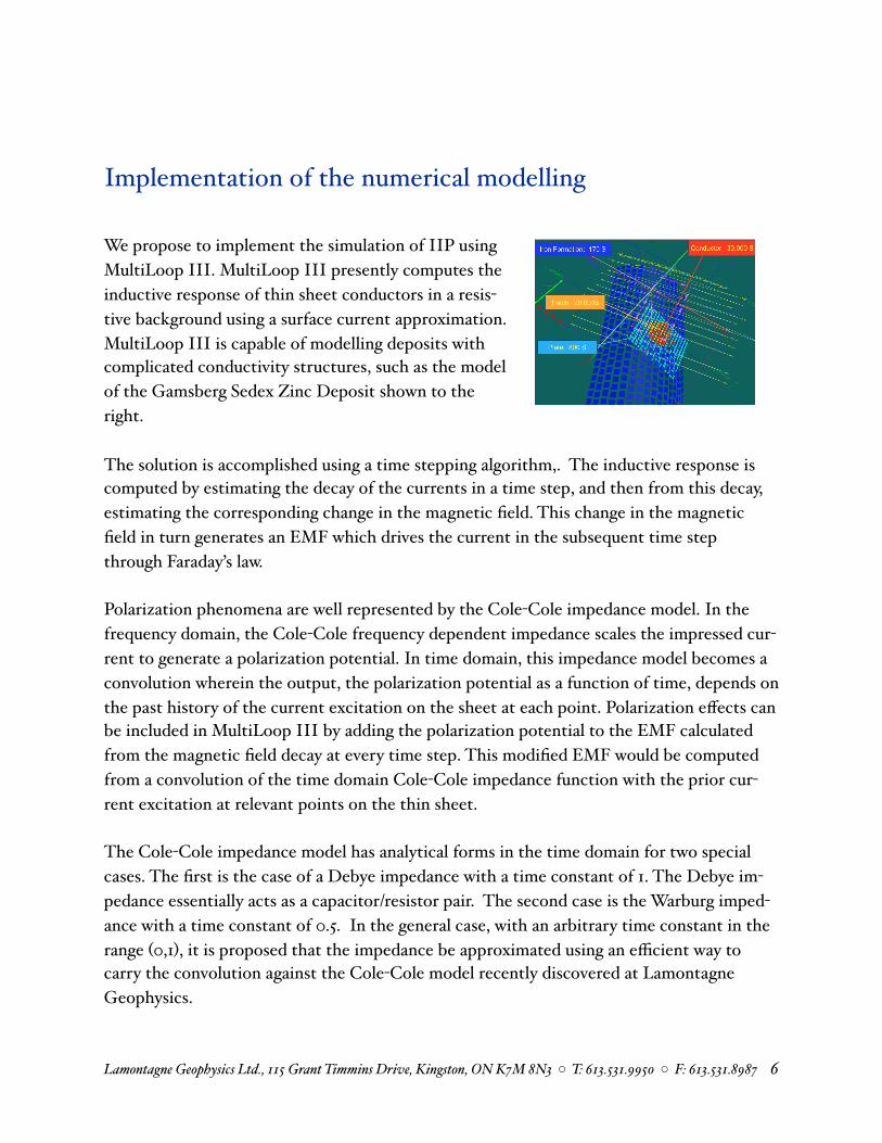
We propose to implement the simulation of IIP using MultiLoop III. MultiLoop III presently computes the inductive response of thin sheet conductors in a resis-tive background using a surface current approximation. MultiLoop III is capable of modelling deposits with complicated conductivity structures, such as the model of the Gamsberg Sedex Zinc Deposit shown to the right.

The solution is accomplished using a time stepping algorithm,. The inductive response is computed by estimating the decay of the currents in a time step, and then from this decay, estimating the corresponding change in the magnetic field. This change in the magnetic field in turn generates an EMF which drives the current in the subsequent time step through Faraday’s law.

Polarization phenomena are well represented by the Cole-Cole impedance model. In the frequency domain, the Cole-Cole frequency dependent impedance scales the impressed cur-rent to generate a polarization potential. In time domain, this impedance model becomes a convolution wherein the output, the polarization potential as a function of time, depends on the past history of the current excitation on the sheet at each point. Polarization effects can be included in MultiLoop III by adding the polarization potential to the EMF calculated from the magnetic field decay at every time step. This modified EMF would be computed from a convolution of the time domain Cole-Cole impedance function with the prior cur-rent excitation at relevant points on the thin sheet.

The Cole-Cole impedance model has analytical forms in the time domain for two special cases. The first is the case of a Debye impedance with a time constant of 1. The Debye im-pedance essentially acts as a capacitor/resistor pair. The second case is the Warburg imped-ance with a time constant of 0.5. In the general case, with an arbitrary time constant in the range (0,1), it is proposed that the impedance be approximated using an efficient way to carry the convolution against the Cole-Cole model recently discovered at Lamontagne Geophysics.


Starting with the Debye case, it is a simple matter to replace the Debye impedance formula with the Warburg impedance formula. With additional development, first a slow, and then a faster, version of the efficient convolution to represent the Cole-Cole model will be imple-mented.

We have to hope that the polarization EMF does not adversely affect the convergence of the solver currently employed in MultiLoop III. There is no way of predicting this until numerical experiments are attempted with simple Debye impedances, which are likely to represent the worst of the encountered cases.

Cost & Development

The total cost of the project is projected to be $60,000 two be divided among the sponsors. Approximately 4-6 sponsors are sought in addition to Lamontagne Geophysics.

Development is to be split into two phases. The first phase will consist of developing the computational algorithm, while the second phase will consist of the implementation of a user interface and testing. Each sponsor will be invoiced 50% for the first phase, and if phase 1 is successful, then for the remaining 50% to develop a user interface and some test cases.

Total project time is estimated to take 4-6 months.

Deliverables

Each sponsor will receive a license to use the IIP software which will be limited to their use for a period of 1 year following delivery of the completed product.


DEVELOPING THE INDUCTIVE INDUCED POLARIZATION METHOD …

Documents

Transcript of DEVELOPING THE INDUCTIVE INDUCED POLARIZATION METHOD …