Developing the Astronomy of Black HoleMergers with Gravitational Waves

Dustin Leininger

August 11, 2014

Contents

1 Introduction 21.1 Future Astronomy . . . . . . . . . . . . . . . . . . . . . . . . 21.2 Data Analysis . . . . . . . . . . . . . . . . . . . . . . . . . . . 3

2 Methods 52.1 NR-Simulation Catalogs . . . . . . . . . . . . . . . . . . . . . 52.2 Principle Component Analysis [1] . . . . . . . . . . . . . . . . 62.3 Bayesian Model Selection and Parameter Estimation [1] [2] . . 92.4 Sky Localization . . . . . . . . . . . . . . . . . . . . . . . . . 12

3 Results 163.1 Sky Localization . . . . . . . . . . . . . . . . . . . . . . . . . 163.2 Bayes Factors . . . . . . . . . . . . . . . . . . . . . . . . . . . 19

4 Conclusions 21

5 Acknowledgements 22

1

Chapter 1

Introduction

1.1 Future AstronomyAs physicists continues to probe further back into the history of the uni-

verse and deeper into the mechanisms of stellar events, there also growsa demand for more observational data. Thus far, the fields of astronomyand observational astrophysics have been dominated primarily by work fo-cusing on physics deductible from observations of the electromagnetic spec-trum. However, there are many instances in which these methods simply failto shed light on phenomenon of interest. Some such examples include thephysics within the core of an exploding star, the evolution of black holes,as well as the mechanics of certain binary stellar systems and their mergers.Fortunately, there are other means of deducing physics concerning these andother cosmic events for which traditional methods fall short.

The detection of gravitational waves would not only provide one of thefinal verifications of Einstein’s theory of general relativity, but also a newobservational resource for astronomy capable of probing phenomenon previ-ously inaccessible by electromagnetic observations. Gravitational waves arepropagating perturbations in spacetime generated by quadrapole momentsin matter. These are normally simply accelerating asymmetric masses in-cluding such things as orbiting binaries or spinning bodies with significantmountains and valleys. The larger the acceleration or the asymmetry, themore significant the perturbation. For these reasons binary black hole sys-tems are likely candidates for gravitational wave observation particularly

2

while in their rapidly orbiting late stage inspirall, merger, and ring downphases.

Since gravitational waves are generated by the motion and distribution ofmass, they can encode and carry physically significant data about the evolv-ing states of their progenitors regardless of their emission of electromagneticradiation. Therefore, gravitational waves offer an alternative method of ob-serving the cosmos allowing for the possibility of achieving unprecedentedinsights into physical processes.

1.2 Data AnalysisIn order to develop a new astronomy, a complete data analysis machinery

must be developed and set in place which can deduce physics from obser-vations. Like observations of electromagnetic radiation, certain informationabout the progenitors of the gravitational waves can be inferred from variousproperties of the waves themselves. Among the properties to be determined,the sky location of progenitor events is of central importance. However, asurprising number of insights might be gained from the analysis of detectedwaves.

Briefly, there are two broad classifications of gravitational waves; contin-uous waves and bursts. The former are generated by events which occuron long time scales which continuously emit gravitational waves throughouttheir evolution. Inspiralling binaries are one such example which can emitgravitational waves for many years. The latter classification refers to progen-itor events which occur on a much shorter time scale. These include eventssuch as supernova which emit gravitational waves with durations on the or-der of seconds or less. Some events may transition from one type to the otherduring their evolution. In the late stage inspirall, merger, and ringdown ofa binary system gravitational waves are produced that are distinct from theearlier stages of the inspirall. Firstly, the amplitude of the waves greatlyincreases during these stages. This means that for binaries with continuouswaves of small amplitude, these late stage events may be all that can bedetected. Lastly, the merger and ringdown occur very quickly and thereforefall into the domain of burst gravitational waves. It is with these kinds of

3

burst waves that the current report is primarily concerned, and more specif-ically the determination of the sky location of their sources. In Fig. 1.1, anexample waveform of this kind can be seen.

Figure 1.1: This is a plot of a simulated gravitational wave signal generatedby a binary black hole system in which the black holes were of equal massand zero spin. As can been seen, the early segment of this wave is veryregular in frequency and amplitude. The time during and before this stageof the systems evolution are a source of continuous gravitational waves. Therecan also been seen a remarkable and rapid increase in both amplitude andfrequency towards the later stages of the systems evolution during which thebinary system merges and rings-down. This region falls under the perviewof burst gravitational wave analysis. For very distant or small systems thismay be the only detectable stage of the entire evolution of the system.

4

Chapter 2

Methods

2.1 NR-Simulation CatalogsGiven the complexity and nature of Einstein’s field equations, many sys-

tems are analytically intractable. Therefore, much work has been done tosolve these systems numerically. The development of data analysis toolsis heavily dependent on these simulations provided by numerical relativ-ity. First, they act as the predictions against which observations must becompared in order to test theory. Second, during the development of thetechniques and tools of data analysis, they act as test data on which an al-gorithm and/or code maybe be tested to check for validity. However, thesesimulations are difficult to construct and can be computationally expensive.Therefore, the available simulations can be limited in variety.

For analysis purposes, the simulated waveforms are usually grouped to-gether into sets called catalogs. These are matrices each column of whichis a different simulated waveform. All of the waveforms in a catalog usuallyshare a certain set of fixed parameters while other parameters are varied soas to created an approximate representative sample of the given set of fixedparameters. In the analysis reported here, three catalogs were implemented.The waveforms from each catalog all came from simulations of binary blackhole systems. All of the waveforms in the first catalog, referred to as theQ-series, came from simulations in which neither of the black holes werespinning. There were 33 waveforms in the Q-series over which the mass ratioof the black holes was varied. The 81 waveforms in the second catalog, called

5

the HR-series, were generated in simulations in which both black holes werespinning at the same rate and for which their spin angular momenta wereparallel to the orbital angular momentum of the system. In this catalog, themass ratio was again varied as was the magnitude of the spins. Lastly, thethird catalog, referred to as the RO3-series, contained 19 waveforms in whichthe spin angular momenta of the black holes were allowed to freely precessduring inspiral. The mass ratio, spin magnitude, and initial angular displace-ment between the spin angular momenta of the black holes were varied ineach waveform (one spin initially parallel to the orbital angular momentumand the other initially askew varied angles).

Work has already been done to successfully enable the identification ofunknown waveforms as belonging to one of these catalogs. This effectivelyallows for the identification of the type of source of the gravitational wave aswell as some of its other parameters. The focus of the work reported here wasto broaden the capabilities of the analysis to include the ability to identifythe sky location of the progenitor allowing for a more complete astronomyof gravitational waves.

2.2 Principle Component Analysis [1]The first step of the analysis used here is Principle Component Analysis

(PCA) which implements a matrix decomposition technique from linear al-gebra called Singular Value Decomposition (SVD) to factor the catalog intomore computationally useful matrices.

Singular Value DecompositionA(mxn) = U(mxm)Σ(mxn)V

T(nxn)

(2.1)

SVD decomposes a matrix A into three factor matrices. The first is oftendenoted by U . It’s columns form what are called the left singular vectorswhich obey the equation c1A = c1σ1 where c1 is the first column of U andσ1 is its corresponding singular value. The third matrix is denoted by V T .The columns of V form the right singular vectors of A and obey the same

6

equations as the the columns of U with the exception that the columns of Voperate on the right of A as indicated by its name. The middle matrix (Σ)is a diagonal matrix whose elements correspond to the singular values of thecolumns of U and V .

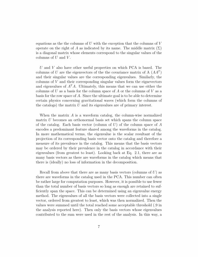
U and V also have other useful properties on which PCA is based. Thecolumns of U are the eigenvectors of the the covariance matrix of A (AAT )and their singular values are the corresponding eigenvalues. Similarly, thecolumns of V and their corresponding singular values form the eignevectorsand eigenvalues of ATA. Ultimately, this means that we can use either thecolumns of U as a basis for the column space of A or the columns of V as abasis for the row space of A. Since the ultimate goal is to be able to determinecertain physics concerning gravitational waves (which form the columns ofthe catalogs) the matrix U and its eigenvalues are of primary interest.

When the matrix A is a waveform catalog, the column-wise normalizedmatrix U becomes an orthonormal basis set which spans the column spaceof the catalog. Each basis vector (column of U) of the column space of Aencodes a predominant feature shared among the waveforms in the catalog.In more mathematical terms, the eigenvalue is the scalar resultant of theprojection of its corresponding basis vector onto the catalog and therefore ameasure of its prevalence in the catalog. This means that the basis vectorsmay be ordered by their prevalence in the catalog in accordance with theireigenvalues (from greatest to least). Looking back at Eq. 2.1, there are asmany basis vectors as there are waveforms in the catalog which means thatthere is (ideally) no loss of information in the decomposition.

Recall from above that there are as many basis vectors (columns of U) asthere are waveforms in the catalog used in the PCA. This number can oftenbe rather large for computation purposes. However, it is possible to use fewerthan the total number of basis vectors so long as enough are retained to suf-ficiently span the space. This can be determined using an eigenvalue energymethod. The eigenvalues of all the basis vectors were collected into a singlevector, ordered from greatest to least, which was then normalized. Then thevalues were summed until the total reached some acceptable threshold (.9 inthe analysis reported here). Then only the basis vectors whose eigenvaluescontributed to the sum were used in the rest of the analysis. In this way, a

7

much smaller computationally tractable approximate basis was constructedwhich still sufficiently spanned the catalogs. The basis vectors used in thefinal analysis are called the Principle Components (PCs). As can be seenin Fig. 2.1, remarkably few PCs (compared to the size of the catalogs) arerequired to span each catalog. In the analysis reported here, 2 PCs wereused on the Q-series analysis, 5 for the RO3-series analysis, and 8 for the HRseries.

If the original catalog is large enough, then U can be considered to be thebasis for all waveforms sharing the same parameters as those in the catalog.As an example, the columns of the normalized U matrix which results fromthe application of PCA to the Q-series catalog may be used as an approximatebasis for all waveforms generated by non-spinning binary black hole systemsand not just those simulations used in the Q-series catalog. In this way, thisalgorithm gains the ability to effectively analyze unsimulated waveforms. Theamazing ability to generalize the available simulations and accurately handleunsimulated waveforms is part of what makes analysis so powerful.

2 4 6 8 10Number of PCs

0.20.30.40.50.60.70.80.91.0

E(k

)

QHRRO3

Figure 2.1: In this figure, the eigen-energy is plotted as a function of thenumber of PCs. Impressively few of the PCs are needed in order to sufficientlyspan the catalogs. Only 2 PCs are required for the Q-series, 5 for the RO3-series, and 8 for the HR series.

8

2.3 Bayesian Model Selection and ParameterEstimation [1] [2]

The second crucial element of analysis reported here is based on BayesianStatistics in which Bayes Theorem pays a central role. Bayes Theorem relatesthe probability the that a hypothesis is true given the data set {Dk} ( calledthe posterior and denoted P (H|{Dk}, I) ) to the probability that the datawould have been observed given that the hypothesis were true ( called thelikelihood and denoted P ({Dk}|H, I) ). This is extremely useful as it isusually much easier to compute the likelihood than the quantity of primaryinterest, the posterior. In Bayes Thm., the posterior is also related to theprobability that the hypothesis is true without support from the data (calledthe prior and denoted P (H|I) ) and the probability that the data wouldhave been observed given no hypothesis (called the evidence and denotedP ({Dk}|I) ). However, the evidence is often ignored as a scale factor tobe computed during normalization after the fact. Another important noteis that at large samples the likelihood almost always dominates the prior.However, both quantities can be of essential importance depending on theproblem at hand.

Bayes TheoremP (H|{Dk}, I) = P ({Dk}|H, I)× P (H|I)

P ({Dk}|I)(2.2)

Bayes Thm. is primarily used as a parameter estimation tool in which theresulting posterior is the probability distribution function of some quantityof interest. In the current analysis the sky locations (right ascension anddeclination) of the source were of primary concern. To ensure an unbiasedposterior, a prior is normally chosen which exhibits maximal ignorance. Thisoften results in the assignment of a flat prior distribution in which eachpossibility is given equal weight. In the analysis reported here, flat priorswere implemented for both the right ascension and declination. Although,it is important to note that a flat prior is not the most unbiased assignmentfor the declination as it will favor the poles. Since the likelihood function so

9

strongly dominates the analysis, this was not seen as a serious error but willbe revisited and revised in future work (for a full length discussion of the skylocalization analysis, see 2.4).

Since the likelihood is meant to be the probability of measuring the datagiven the hypothesis to be true, it is often modeled after the expected noiseof the observed data. For an uncorrelated data set with Gaussian noise, thelikelihood is simply the product over the Gaussian noise on each data pointin the set. The addition of each data point in the set alters the posteriordistribution until it reflects the estimate preferred by the data. The Like-lihood function used in this analysis is Eq. 2.3. The "model" term in Eq.2.3 is a reconstruction from the PCs using parameters which are at first ran-domly chosen but then begin to converge to higher likelihood values using theNested Sampling Algorithm described in [2]. For computational purposes,the logarithm of the likelihood was computed which simply and convenientlychanges the product to a sum.

Likelihood Functionlog(L) = −2 ∆F ×

∑i

(wave(i)−model(i))2

noise(i)(2.3)

In earlier work, which preceded this report but with which this report isstill concerned, the focus was to determine which among the catalogs aninjected signal most likely belongs thereby determining the most likely typeof source (among other parameters). This can be done by evaluating the ratioof two posteriors, the first in which the "model" in Eq. 2.3 was generatedby the PCs of one catalog, and the second in which the "model" in Eq. 2.3was generated using the PCs of a second catalog. By assuming a priorithat the waveform has an equal probability of being from either catalog, thepriors for the posteriors of the two catalogs become equal and cancel out inthe ratio. Furthermore, the evidence in the denominator of each posteriorcan be ignored at this stage as a scale factor. This leaves only the ratio ofthe likelihoods which is often referred to as the Bayes Factor. Also, in theliterature, the proposition "that the waveform belongs to the first catalog" is

10

referred to as Hypothesis 1 and is usually denoted H1. A similar conventionis adopted for the proposition "that the waveform belongs to the secondcatalog". Again, it is common to compute the logarithm of the Bayes Factorsuch that a positive BH1H2 in Eq. 2.4 is consistent with a preference in thedata for H1 and a negative BH1H2 with a preference for H2.

Bayes FactorBH1H2 = P ({Dk}|H1, I)

P ({Dk}|H2, I))(2.4)

The probability that a waveform belongs to a given catalog i ( P ({Dk}|Hi, I)) is determined by the fit and coefficients of the linear combination of the PCsbelonging to that catalog used in the likelihood function. This means thatP ({Dk}|Hi, I) is a multi-parameter probability. Therefore, what is needed isa method of reducing the multiple posteriors (one for each coefficient in thelinear combination) into a single posterior for the entire hypothesis. This isdone in two steps. The first is to use Eq. 2.5 known as the Product Rulewhich states that the probability, given only that the hypothesis is true, ofobserving data {Dk} corresponding to a fixed set of parameters (in this casecoefficients) {θi} is equal to the product of the probability that the datawould have been observed, given the parameters and the hypothesis, and theprobability that given that the hypothesis were true given that the set ofparameters.

Product RuleP ({Dk}, {θi}|H) = P ({Dk}|{θi}, H)× P ({θi}|H)

(2.5)

The second step to computing ( P ({Dk}|Hi) ) is Eq. 2.6 and is called theMarginalization Rule. It allows for the elimination the dependence on {θi} inP ({Dk}, {θi}|Hi) by summing over all possible values of the elements of {θi}.Since the values of the coefficients vary continuously, the summation becomes

11

an integral. The limits of integration are determined by the upper and lowerbounds on the prior for the parameter estimation on the coefficients.

Marginalization RuleP ({Dk}|Hi) =

∫...

∫iP ({Dk}|{θi}, Hi)× P ({θi}|Hi) d{θi}

(2.6)

By sampling the likelihood and prior, it is ultimately this integral whichis computed by the Nested Sampling Algorithm. As a final note, the BayesFactor computed in actual analyses is always the ratio of Hi to noise whichis simply checking to see if there is any signal present at all. To discernthe overall Bayes Factor between two hypotheses, simply take the differencebetween their respective Bayes Factors.

2.4 Sky LocalizationAs mentioned earlier, the primary focus of the work done this summer was

to broaden the capabilities of the existing analysis to include estimates ofthe sky locations (including right ascension and declination) of the sourcesof gravitational waves generated by binary black hole systems. In order todetermine the sky location, multiple detectors must be used in the analysis.This introduces new complications to the analysis including the time delaybetween various detectors and the different antenna response patterns of thedetectors which were the primary focus in this report.

First, the time shift between the different detectors physically originatesin their different locations on the surface of the earth. A single wave whichpasses through multiple detectors will reach each detector at a slightly differ-ent time. The detected signals therefore need to be time shifted and alignedsuch that they are able to compared. In the analysis, the center of the earthwas taken to be the origin. Since each detector remains stationary on thesurface of the earth with respect to the Earth’s center, the time shift fromthe center to a given detector remains constant. Once the simulated signalis injected at each detector, a short segment of code simply applies the cal-

12

culated time shifts of each detector to their respective injections effectivelytime shifting them all to the center of the earth.

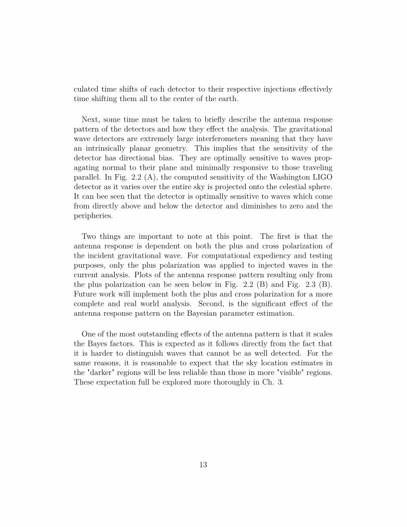
Next, some time must be taken to briefly describe the antenna responsepattern of the detectors and how they effect the analysis. The gravitationalwave detectors are extremely large interferometers meaning that they havean intrinsically planar geometry. This implies that the sensitivity of thedetector has directional bias. They are optimally sensitive to waves prop-agating normal to their plane and minimally responsive to those travelingparallel. In Fig. 2.2 (A), the computed sensitivity of the Washington LIGOdetector as it varies over the entire sky is projected onto the celestial sphere.It can bee seen that the detector is optimally sensitive to waves which comefrom directly above and below the detector and diminishes to zero and theperipheries.

Two things are important to note at this point. The first is that theantenna response is dependent on both the plus and cross polarization ofthe incident gravitational wave. For computational expediency and testingpurposes, only the plus polarization was applied to injected waves in thecurrent analysis. Plots of the antenna response pattern resulting only fromthe plus polarization can be seen below in Fig. 2.2 (B) and Fig. 2.3 (B).Future work will implement both the plus and cross polarization for a morecomplete and real world analysis. Second, is the significant effect of theantenna response pattern on the Bayesian parameter estimation.

One of the most outstanding effects of the antenna pattern is that it scalesthe Bayes factors. This is expected as it follows directly from the fact thatit is harder to distinguish waves that cannot be as well detected. For thesame reasons, it is reasonable to expect that the sky location estimates inthe "darker" regions will be less reliable than those in more "visible" regions.These expectation full be explored more thoroughly in Ch. 3.

13

Figure 2.2: In (A) the total response pattern of the Hanford LIGO detectorincluding both plus and cross polarization contributions as projected ontothe celestial sphere. It is clear that detector is most sensitive to the areason the sphere which lie directly above and beneath it and attenuates tozero along it periphery. In (B) the antenna response pattern of the HanfordLIGO detector resulting from only the plus polarization contribution. Thisis a much less physical result as it depicts only the detector’s response tothe plus polarization components of prospective gravitational waves as theirsources vary over the sky.

14

Figure 2.3: In (A) the combined total response pattern of the HanfordLIGO detector, Livingston LIGO detector, and the Virgo detector includingboth plus and cross polarization contributions is projected onto the celestialsphere. The combination of three detectors has significantly increased thevisibility. Particularly, there is no longer a connected bind of blind spacewhich wraps around he entire sphere. In (B) the antenna response pattern ofthe aforementioned trio of detectors resulting from only the plus polarizationcontribution is projected onto the celestial sphere. Again, this is a much lessphysical result as it depicts only the detectors’ response to the plus polar-ization components of prospective gravitational waves as their sources varyover the sky. However, this is the only component used in the analysis pre-sented later in this report and this is therefore the antenna response patternimplemented in the analysis.

15

Chapter 3

Results

In this analysis, 48 sky locations were selected for injection sites using theprogram MEALPix (more information about MEALPix can be found athttp://www.gwastro.org/for20scientists/mealpix-matlab-healpix-interface-1).Each waveform from each catalog was injected at each of the 48 sky loca-tions and then compared against each of the three catalogs in the analysis.This ultimately resulted in 6500+ jobs which are currently running on thecomputing clusters at Caltech. As of the time of writing of this report, onlyroughly one sixth of the jobs had finished. Fortunately, the analysis outputdata as it progressed. At least partial data was produced concerning all skylocations of all waveforms of the RO3 catalog. Since the rest of the data wassimply too incomplete, all of the preliminary results presented here will arerestricted to the analysis of the RO3 catalog.

3.1 Sky LocalizationAs mentioned earlier the aim of this project was to implement sky location

estimates into the analysis. In Ch. 2.4 above, the method for constructingthe estimates for the right ascension and declination is described. Each it-eration of the nested sampling generates an estimate of the sky location. Ahistogram of the estimates generates a distribution of likely values examplesof which can be seen below in Fig. 3.1 and Fig. 3.2. The waveforms wereinjected with an SNR of 50 which is particularly high for real world simula-tions but appropriate to the early stage testing reported here which simplydemonstrates the ability to determine sky location.

16

Figure 3.1: Above is plotted a histogram of all the estimates of the declinationof the 10th waveform in the RO3 catalog on its entire range of possible valuesfrom -π2 to π

2 . The flat red line in the diagram is the prior distribution. Ascan been seen, the distribution is sharply peaked about the best estimate of.3611 which is remarkably close to the true value for the injection which was.3398

These preliminary results seem to indicate that the analysis is able todetermine the sky location. The impressive accuracy of the estimates is ofcourse influenced by the high SNR used in the injections. However, it wasonly the scope of this report to demonstrate the ability to deduce sky locationat all.

While the variation in the sky location estimates do seem to correlateas expected with the antenna pattern, the precision of the estimates andthe sparse sampling of the sky made it difficult to graphically represent.However, the difference in the actual and estimated sky locations can be

17

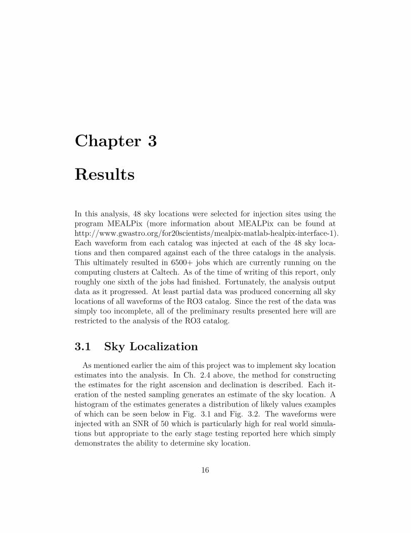
Figure 3.2: Above is plotted a histogram of all the estimates of the declinationof the 10th waveform in the RO3 catalog on its entire range of possible valuesfrom 0 to 2π. Although not depicted here, the prior distribution for thisestimate was similarly flat and very small in amplitude compared to thehistogram. Similar to Fig. 3.1, the distribution is sharply peaked about thebest estimate of 3.1385 which is again very close to the true value for theinjection which was 3.1415

seen as projected onto the celestial sphere in Fig. 3.3 alongside the antennaresponse pattern used in the analysis and described above in Ch. 2.4.

While these early results seem to bode well for the success of the imple-mentation of sky localization to the analysis much work remains to be doneto fully verify the success or failure. When the data is complete, a morethorough and rigorous analysis of the data will be done. Afterwords, thenumber of sky locations on the analysis will be increased to verify the suc-cessful implementation of the antenna response pattern once both plus andcross polarizations are implemented.

18

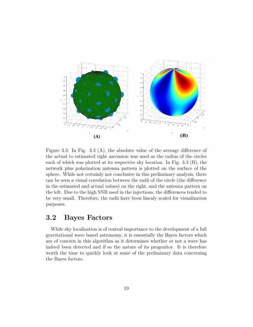
Figure 3.3: In Fig. 3.3 (A), the absolute value of the average difference ofthe actual to estimated right ascension was used as the radius of the circleseach of which was plotted at its respective sky location. In Fig. 3.3 (B), thenetwork plus polarization antenna pattern is plotted on the surface of thesphere. While not certainly not conclusive in this preliminary analysis, therecan be seen a visual correlation between the radii of the circle (the differencein the estimated and actual values) on the right, and the antenna pattern onthe left. Due to the high SNR used in the injections, the differences tended tobe very small. Therefore, the radii have been linealy scaled for visualizationpurposes.

3.2 Bayes FactorsWhile sky localization is of central importance to the development of a full

gravitational wave based astronomy, it is essentially the Bayes factors whichare of concern in this algorithm as it determines whether or not a wave hasindeed been detected and if so the nature of its progenitor. It is thereforeworth the time to quickly look at some of the preliminary data concerningthe Bayes factors.

19

Below can be seen a similar plot to that in Fig. 3.3. However, in thisplot, the Bayes factors of signal to noise have been averaged and used as theradii of circles which are again plotted at their respective sky locations onthe sphere.

Figure 3.4: I this plot, the average Bayes factor across all wave forms andcatalogs has been used as the radii of the circles plotted at the respective skylocations. The size of the circle is therefore a rough indicator of the analsis’ability to distinguish signal from noise at the given sky location. Again, thisanalysis is influenced by the high SNR. However, the purpose of this plot isagain to show the effect of the antenna response pattern on the analysis.

20

Chapter 4

Conclusions

Given the limited nature of the data presented here, it would be inappro-priate to try and draw any hard conclusions. However, It does appear ingeneral that the analysis is capable of deducing sky locations and correctlyimplementing the combined antenna response patterns as well as other tech-nical problems inherent in the implementation of multiple detectors in theanalysis.

21

Chapter 5

Acknowledgements

I would like to thank Dr. Ik Siong Heng how oversaw my work at GlasgowUniversity as well as James Clark and Nick Mangini at the University ofMassachusetts as Amherst for their help and guidance during this assignment.

22

References

[1] I.S. Heng P. Kalmus J. Louge, C.D. Ott and J.H.C Scargill. InferringCore-Collapse Supernova Physics with Gravitational Waves. PHYSICALREVIEW D, 86.

[2] D.S. Sivia. Data Analysis: A Baysian Tutorial. Oxford University Press,second edition, 2006.

23