DEVELOPING FRAGILITY FUNCTIONS FOR … within the city of Banda Aceh, using high-resolution...

August 13, 2009 14:8 WSPC/101-CEJ 00200

Coastal Engineering Journal, Vol. 51, No. 3 (2009) 243–273c© World Scientific Publishing Company and Japan Society of Civil Engineers

DEVELOPING FRAGILITY FUNCTIONS FOR TSUNAMI

DAMAGE ESTIMATION USING NUMERICAL MODEL AND

POST-TSUNAMI DATA FROM BANDA ACEH, INDONESIA

SHUNICHI KOSHIMURA

Disaster Control Research Center, Graduate School of Engineering,Tohoku University, Aoba 6–6–11–1104, Aramaki,

Aoba–Ku, Sendai 980–8579, [email protected]://www.tsunami.civil.tohoku.ac.jp

TAKAYUKI OIE

Pacific Consultants Co., LtD., Shintera 1–4–5,Wakabayashi–Ku, Sendai 984–0051, Japan

[email protected]://www.pacific.co.jp/

HIDEAKI YANAGISAWA∗ and FUMIHIKO IMAMURA†

Disaster Control Research Center, Graduate School of Engineering,Tohoku University, Aoba 6–6–11–1104, Aramaki,

Aoba–Ku, Sendai 980–8579, Japan∗[email protected]

†[email protected]

Received 19 September 2008Revised 21 February 2009

Fragility functions, as new measures for estimating structural damage and casualties dueto tsunami attack, are developed by an integrated approach using numerical modeling oftsunami inundation and GIS analysis of post-tsunami survey data of the 2004 Sumatra–Andaman earthquake tsunami disaster, obtained from Banda Aceh, Indonesia. The fragilityfunctions are expressed as the damage probabilities of structures or death ratio with regardto the hydrodynamic features of tsunami inundation flow, such as inundation depth, currentvelocity and hydrodynamic force. They lead to the new understandings of the relationshipbetween local vulnerability and tsunami hazard in a quantitative manner.

Keywords: Fragility function; vulnerability; tsunami inundation; The 2004 Sumatra–Andaman earthquake; Banda Aceh.

243

August 13, 2009 14:8 WSPC/101-CEJ 00200

244 S. Koshimura et al.

1. Introduction

The tsunami generated by the 26 December 2004 Sumatra–Andaman earthquake

(Mw = 9.0–9.3) caused extensive damage to coastal areas along the Indian Ocean.

Since the event occurred, various efforts to investigate the impact of tsunami have

been made. The post-tsunami survey teams (ITST: International Tsunami Survey

Team) were widely deployed and reported the tsunami heights, extent of inunda-

tion zone and damage, e.g. [Borrero, 2005], [Matsutomi et al., 2006], [Tsuji et al.,

2006], [Fujima et al., 2006] and [Satake et al., 2006]. These efforts also have led to

the new understandings of local aspects of tsunami inundation flow and damage

mechanisms. Matsutomi et al. [2006], Tomita et al. [2006] and Yamamoto et al.

[2006] discussed some mechanisms of tsunami damage on structures during their

post-tsunami surveys. For instance, it was found that the tsunami with more than

2 m of its inundation depth potentially destroys houses made of mortar and bricks

[Yamamoto et al., 2006]. However, their findings are based on the inspection of lo-

cal aspects of tsunami damage and have difficulties to identify the “vulnerability”

in a quantitative manner. Vulnerability information is associated with multitude

of uncertain sources, such as hydrodynamic features of tsunami inundation flow,

countermeasures, structural characteristics, population, land use, and any other site

conditions. And it should be led through some statistical approach considering the

uncertainties. In that sense, Shuto [1993] discussed the damage possibility of houses

with regard to the tsunami intensity scale or local tsunami height collected from

the documents of historical tsunamis in Japan. Shuto’s tsunami intensity scale and

damage possibility have been widely used as a measure of tsunami damage. However,

as he concluded, degree of damage may change according to the uncertainties sug-

gested above. Also, developing a vulnerability information requires great amount of

damage data, and post-tsunami survey hardly provides satisfactory amount of them

because of the limitation of time and human resources during the survey.

Recent advances of remote sensing technologies expand capabilities of detecting

spatial extent of tsunami affected areas and damage on structures. The highest

spatial resolution of optical imageries from commercial satellites is up to 60–70

centimeters (QuickBird owned by DigitalGlobe, Inc.) or 1 meter (IKONOS operated

by GeoEye). Since the 2004 event, these satellites have captured the images of

tsunami–affected areas and were used for disaster management activities including

emergency response and recovery. Vu et al. [2007] developed a framework to integrate

optical satellite imageries and digital elevation data in mapping tsunami affected

areas. Miura et al. [2006] visually interpreted the structural damage using IKONOS

imageries of pre and post-tsunami in Sri Lanka. Throughout the visual inspection,

they classified the damage of 20,000 buildings into three categories — collapsed,

partially-collapsed and negligible to slight damage. The most significant advantage

of using high-resolution satellite imagery is the capability of detecting structural

damage individually, and enables us to comprehend the structural damage and its

extent in regional scale where post-tsunami field survey cannot get through.

August 13, 2009 14:8 WSPC/101-CEJ 00200

Developing Fragility Functions for Tsunami Damage Estimation 245

The primary objective of this study is to identify a regional vulnerability against

tsunami disaster, by developing fragility functions expressed as the relationship be-

tween damage probability on structures of human lives and hydrodynamic features

of tsunami inundation. To develop the fragility functions, we focus on Banda Aceh

city of northern Sumatra, Indonesia, which was caused more than 70,000 casualties

and 12,000 of house damages during the 2004 event, e.g. [JICA, 2005]. Traditionally,

fragility functions (or fragility curves) have been developed in performing seismic

risk analysis of structural system to identify structural vulnerability against strong

ground motion by utilizing damage data associated with past earthquakes and spa-

tial distribution of observed or simulated seismic responses [Murao and Yamazaki,

2000]. And it has been implemented to estimate structural damage against seismic

risks in which various uncertain sources such as seismic hazard, structural charach-

teristics, soil-structure interaction are involved [Shinozuka et al., 2000].

In principle, the development of fragility functions for tsunami damage estima-

tion requires synergistic use of tsunami hazard information and damage data. To

obtain tsunami hazard information such as inundation depth and current veloc-

ity, we perform a numerical modeling of the 2004 Sumatra–Andaman earthquake

tsunami within the city of Banda Aceh, using high-resolution bathymetry and to-

pography data. The model results, including the tsunami source model (initial sea

surface displacement), extent of inundation zone, inundation depth and current ve-

locity, are validated by measured or field data, and are confirmed to be adequate

for the purpose of fragility function development. In terms of the damage data

including structural damage and casualties, we use the result of visual detection

from the high-resolution satellite imageries and reported number of casualties. In-

tegrating these results, we develop the fragility functions for structural damage and

casualties throughout the statistical analysis under the assumption that they can

be represented by normal or lognormal distribution functions with two statistical

parameters (median and standard deviation of the samples).

2. Developing Tsunami Source Model

2.1. Tectonic background

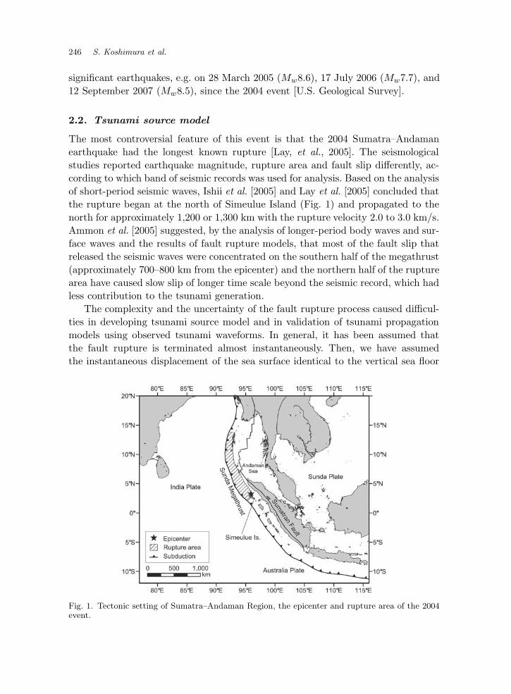
The 2004 Sumatra–Andaman earthquake occurred along the Sunda megathrust. The

Sunda megathrust runs southward from Bagladesh, along Sunda and Java trench

and all the way to Australia, and is the plate interface between the Indian/Australian

oceanic plate subducting beneath the Sunda plate (Fig. 1). The subducting plate

is moving north–northeast at a rate of approximately 50 to 57 mm/year [Sieh,

2007] and the strain accumulation over hundreds of years were suddenly relieved as

a series of great fault ruptures. Although the rupture length is still controversial,

more than 1,000 km of the megathrust caused the great earthquake of magnitude 9.0

to 9.3 and made this event the largest in the past 40 years. The strain release along

the Sunda megathrust is believed to be still highly active and have caused several

August 13, 2009 14:8 WSPC/101-CEJ 00200


significant earthquakes, e.g. on 28 March 2005 (Mw8.6), 17 July 2006 (Mw7.7), and

12 September 2007 (Mw8.5), since the 2004 event [U.S. Geological Survey].

2.2. Tsunami source model

The most controversial feature of this event is that the 2004 Sumatra–Andaman

earthquake had the longest known rupture [Lay, et al., 2005]. The seismological

studies reported earthquake magnitude, rupture area and fault slip differently, ac-

cording to which band of seismic records was used for analysis. Based on the analysis

of short-period seismic waves, Ishii et al. [2005] and Lay et al. [2005] concluded that

the rupture began at the north of Simeulue Island (Fig. 1) and propagated to the

north for approximately 1,200 or 1,300 km with the rupture velocity 2.0 to 3.0 km/s.

Ammon et al. [2005] suggested, by the analysis of longer-period body waves and sur-

face waves and the results of fault rupture models, that most of the fault slip that

released the seismic waves were concentrated on the southern half of the megathrust

(approximately 700–800 km from the epicenter) and the northern half of the rupture

area have caused slow slip of longer time scale beyond the seismic record, which had

less contribution to the tsunami generation.

The complexity and the uncertainty of the fault rupture process caused difficul-

ties in developing tsunami source model and in validation of tsunami propagation

models using observed tsunami waveforms. In general, it has been assumed that

the fault rupture is terminated almost instantaneously. Then, we have assumed

the instantaneous displacement of the sea surface identical to the vertical sea floor

Fig. 1. Tectonic setting of Sumatra–Andaman Region, the epicenter and rupture area of the 2004event.

August 13, 2009 14:8 WSPC/101-CEJ 00200


displacement. Because of the long extent of fault rupture and long duration of rup-

ture process during the 2004 event, this assumption may not be applicable when

developing tsunami source models. Considering the dynamic effects of fault rupture

has been one of the major issues for developing tsunami source model of the 2004

Sumatra–Andaman earthquake.

Fujii and Satake [2007] used the tsunami waveforms observed by twelve distant

tide gauges in Indian Ocean and sea surface heights measured by three satellite

altimetries [Gower, 2007], and determined the tsunami source model by the inver-

sion analysis with different rupture velocities from 0.5 to 3.0 km/s. Their results

suggest that the computed tsunami waveforms at distant locations are influenced

by changing rupture velocity especially at the tide gauge stations in Sri Lanka and

along the east coast of India, and their best proposal is 1.0 km/s as uniform rupture

velocity within the entire rupture area. Since most of the observed tsunami data

used through their inversion analysis are associated with the northern part of fault

rupture, which seismological research implies slow slip, their estimation is consistent

with the observed features of tsunami waveforms at the tide gauges. However, at

the same time, the result of Fujii and Satake [2007] also suggests no significant dif-

ference of modeled tsunamis account for the satellite altimetry data, when changing

the rupture velocity. This is because the sea surface heights measured by the satellite

altimetries were associated with the tsunami from the southern part of the source

area, and implies that the dynamic process of the southern part of fault rupture

might not strongly affect tsunami waveforms. Other previous studies on tsunami

source focusing on dynamic process of fault rupture suggest variety of rupture ve-

locities, e.g. [Tanioka et al., 2006] (rupture velocity v = 1.7 km/sec), [Hirata et al.,

2006] (v = 0.7 km/sec) and [Piatanesi and Lorito, 2007] (v = 2.0 km/sec), while

seismological studies suggest higher, e.g. [Ammon et al., 2005] (v = 2.5 km/sec) and

[Ishii et al., 2005] (v = 2.8 km/sec). Therefore, the dynamic effects on fault rupture

is still under controversy and may not be well resolved only from tsunami data.

Our major concern is not to develop the tsunami source model which accounts for

all the observed tsunami that features in the Indian Ocean, but for the local tsunami

inundation in the city of Banda Aceh. Thus, the unknown feature of dynamic effects

of fault rupture, such as rupture velocity and rise time, are not considered. Fig-

ure 2 indicates the fault geometries inferred from the tectonic setting, e.g. [Chlieh

et al., 2007], [Dasgupta et al., 2003] and [Sieh, 2007], and aftershock area during

one month since the main shock occurred. We divide the entire rupture area into

6 fault segments dipping eastward resulting a total rupture area of 1,155 km by

150 km. The inferred fault geometry is similar to our previous model [Oie et al.,

2006], but the present study discusses more precisely. As shown in the figure, Banda

Aceh is located at the northern end of Sumatra Island and is likely to be affected

by the tsunami from southern three sub-fault segments. For model constraints, we

mainly use two kinds of data to determine the fault dislocations; Jason-1 altimetry

data [Gower, 2007] for the southern three sub-faults (fault 1–3), and the vertical

August 13, 2009 14:8 WSPC/101-CEJ 00200


Fig. 2. Inferred fault geometries of the 2004 Sumatra–Andaman earthquake.

displacement field revealed by satellite radar imagery [Tobita et al., 2006] and field

measurement [Rajendran et al., 2007] for the entire displacement field (fault 1–6).

Table 1 indicates the resultant fault parameters of 6 sub-faults, determined with the

constraints described above.

Jason-1 is a mission satellite launched by National Aeronautics and Space Ad-

ministration (NASA, United States) and Centre National d’Etudes Spatiales (CNES,

France) and have captured the sea surface of traveling tsunami along the track ap-

proximately two hours after the earthquake. As Gower [2007] reported, this became

the first example for satellite remote sensing to detect the traveling tsunamis in mid-

ocean. Figure 3 shows the track of Jason-1 (track 109) on 26 December 2004 and the

tsunami height along the track which was extracted by Hayashi [2007] to remove the

effect of tide and wind waves. Also, in the figure, the snapshot of modeled tsunami

August 13, 2009 14:8 WSPC/101-CEJ 00200


Table 1. Dimensions of the faults and tsunami source parameters for the 2004 Suma-tra–Andaman earthquake tsunami. n indicates the number of fault segment, which increasesfrom south to north along the strike direction and corresponds to the fault number shown inFig. 2. H is the depth of the upper edge of each fault segment. L is the strike length, W isthe downdip width, and D is the fault displacement.

Segment n H (km) L (km) W (km) Strike (◦) Dip (◦) Slip (◦) D (m)

1 10 200 150 323 15 90 14.02 10 125 150 335 15 90 12.63 10 180 150 340 15 90 15.14 10 145 150 340 15 90 7.05 10 125 150 345 15 90 7.06 10 380 150 7 15 90 7.0

Fig. 3. (a) The track of Jason-1 on 26 December 2004. The modeled tsunami at 2 hours after theearthquake is also shown in the figure. Note that Jason-1 spent approximately 8.3 minutes to flyover the track from 5◦S to 20◦N. (b) The measured sea surface height along the track. The seasurface value in the plot is after the extraction by Hayashi [2007].

2 hours after the earthquake is shown for the explanation of how Jason-1 captured

the sea surface profile of traveling tsunami. We can see, from the figure, Jason-1

clearly detected the sea surface of tsunami front propagating southward from 3◦S to

5◦S in latitude, which is critical to determine the southern part of tsunami source

model.

August 13, 2009 14:8 WSPC/101-CEJ 00200


98 E

98 E

96 E

96 E

94 E

94 E

92 E

92 E

90 E

90 E

8 N 8 N

6 N 6 N

4 N 4 N

2 N 2 N0 100 200 300 400 500km

Fault 1

Fault 2

Fault 3

Plate boundary

Fig. 4. Vertical sea surface displacement field by each sub-fault’s rupture with unit dislocation(1 m). The contour interval is 0.1 m. The solid lines for uplift and the dashed lines for subsidence.

In order to develop the tsunami source model that accounts for captured tsunami

front by Jason-1, we focus on the southern three sub-faults and calculate the tsunami

propagation initiated at each sub-fault with unit dislocation of 1 m. Then, the dis-

location of each sub-fault is determined by adjusting each sub-fault’s dislocation

to be consistent with Jason-1 data. Figure 4 indicates the vertical sea surface dis-

placement field of each sub-fault’s rupture with unit dislocation, calculated by the

theory of Mansinha and Smylie [1971]. For tsunami modeling, we apply the finite

difference method of the linear shallow-water wave theory with Coriolis force in

a spherical co-ordinate system, which was primarily developed by Nagano et al.

[1991], and we use the 1-arc-minute (approximately 1,800 m) digital bathymetry

grid (GEBCO) distributed by British Oceanographic Data Centre [1997] with the

time step of 3 seconds to satisfy the stability condition. The total reflection condi-

tion at the boundary between land and sea, and the free radiation condition at the

open-ocean boundary are applied respectively.

Figure 5 indicates the plot of modeled tsunami heights along Jason-1 track,

initiated by each sub-fault (southern three sub-faults) with unit dislocation (1 m),

and synthetic sea level (solid line). Also in the figure, Jason-1 data is plotted for

the comparison. By this figure, the contribution of each sub-fault in forming mid-

ocean sea surface can be clearly understood. For instance, the first peak (peak 1)

propagating to the south is mostly associated with the tsunami initiated by the

southern two faults (fault 1 and 2). Also, the second peak is formed as the result of

interaction of tsunamis from the second and third faults (fault 2 and 3).

August 13, 2009 14:8 WSPC/101-CEJ 00200


��

��

��

��

��

� � ! � " � # $

%'&)('* +�,%'&)('* + -.'/)0'1 23465'798;:=<>8@? A

B9C'DFE)GIH�J

KMLINOQPSR O>T=OUR9V@WYX

Z=[>\@] \;^=_'`ba_'`'c)d`>`Ue

f�gih

j�kml nIo'p)qsr nIo'p)qut

Fig. 5. (a) Modeled tsunami heights along Jason-1 track, initiated by each sub-fault with unitdislocation (1 m), and synthetic sea level (solid line). (b) Measured sea surface height by Jason-1.

On the other hand, dislocations of northern three sub-faults (fault 4–6) are deter-

mined only by considering total seismic moment and uplift and subsidence patterns

of island arcs which Tobita et al. [2006] reported through the analysis of satellite

radar imageries of pre and post-tsunami along the subduction zone. Figure 6 il-

lustrates the computed vertical displacement field of sea bottom/land surface and

the detected land deformation patterns by Tobita et al. [2006], and it represents

that the present tsunami source model is consistent with the observed deformation

pattern along the island arcs. However, note that the northern extent of tsunami

source and the amount of vertical deformation is still unknown. Thus, the present

tsunami source model may not be appropriate to discuss the overall tsunami fea-

tures in the entire Indian Ocean. The resulting seismic moment is calculated to be

M0 = 5.24 × 1022 Nm (the moment magnitude Mw = 9.08), assuming a uniform

shear modulus of the crust as µ = 3.0 × 1010 N/m2. The maximum uplift and

subsidence are calculated to be 6.66 and 3.09 m respectively.

Figure 7 shows the comparison of modeled and measured sea levels along Jason-

1 track. The modeled and measured sea levels are fairly in good agreement. Es-

pecially in terms of the tsunami front propagating southward, the model result

perfectly matches with the observed tsunami (5 to 6◦S). However, a small discrep-

ancy is recognized for the second peak. Because of the absence of the second peak’s

measurement, there is a limitation to determine where the exact peak is, and the

modeled tsunami looks a little overestimated around the second peak. Also, the

phase difference between the modeled and measured tsunami is apparent around

the second peak. This may be resolved when considering the dynamic process of

fault rupture, i.e. the second and third fault ruptures might be initiated with the

August 13, 2009 14:8 WSPC/101-CEJ 00200


Fig. 6. (a) Computed coseismic displacement of sea bottom and land surface as the present tsunamisource model. Contour interval is 0.5 m. The solid lines for uplift and the dashed lines for subsidence.(b) Detected land deformation by the analysis of satellite radar imageries after Tobita et al. [2006].The area trimmed by black solid line is subsided and gray solid line is uplifted.

� ��

� ��

��

��

��

��

�� "!$#

%'&�(") ("*'+-,/.�+0,-1�23,�,54

687090:�; :09<'=0>@?�A�B�C

Fig. 7. Comparison of measured and modeled tsunami heights along Jason-1 track.

August 13, 2009 14:8 WSPC/101-CEJ 00200


time delay behind the rupture of the southern most fault. In addition, note that the

present model results are based on the linear shallow-water wave theory and may

not be appropriate for the discussion of the tsunami waveforms at later phase, as

addressed by Shigihara and Fujima [2006].

3. Numerical Modeling of Tsunami Inundation

3.1. Numerical model set-up

We perform the numerical modeling of tsunami inundation in the city of Banda Aceh

by assuming the source model presented above. A set of non-linear shallow water

Eqs. (1) to (3) are discretized by the Staggered Leap-frog finite difference scheme

[Imamura, 1995] with bottom friction in the form of Manning’s formula according

to the land use condition (Table 2).

∂η

∂t+

∂M

∂x+

∂N

∂y= 0 (1)

∂M

∂t+

∂

∂x

(

M2

D

)

+∂

∂y

(

MN

D

)

= −gD∂η

∂x−

gn2

D7/3M

√

M2 + N2 (2)

∂N

∂t+

∂

∂x

(

MN

D

)

+∂

∂y

(

N2

D

)

= −gD∂η

∂y−

gn2

D7/3N

√

M2 + N2 (3)

where

M =

∫ η

−hudz (4)

N =

∫ η

−hvdz (5)

D = η + h (6)

M and N are the discharge flux of x and y direction respectively, η is the water

level and h is the water depth above the mean sea level.

The merged bathymetry and topography grids for regional tsunami propagation

and inundation models are created by compilation of GEBCO data, the local bathy-

metric charts of northern Sumatra (1:500,000 and 1:125,000), the land elevation

Table 2. Values of Manning’s roughness coefficient n(after Kotani et al. [1998]).

Smooth ground 0.020Shallow water area or natural beach 0.025Vegetated area 0.030Populated area 0.045Densely populated area Equation (7)

August 13, 2009 14:8 WSPC/101-CEJ 00200


Fig. 8. The computational domain for the model of tsunami propagation and inundation to thecity of Banda Aceh. The grid size varies 1860, 620, 207, 69 and 23 m, from (a) to (e), constructinga nested grid system. The water depth in the regions (a) to (d) and the land elevation in (e) areindicated by gray scale. And only in (e), the water depth is shown by the contours with every 10 m.

data obtained by SRTM [Rabus et al., 2003] (Shuttle Radar Topography Mission)

and the digital photogrammetric mapping [JICA, 2005]. The grid size varies from

1,860 to 23 m from the source region to the coast/land of Banda Aceh, constructing

a nested grid system as shown in Fig. 8.

Especially for modeling tsunami inundation in densely populated region, we ap-

ply the resistance low with the composite equivalent roughness coefficient according

to land use and building conditions, e.g. [Kotani et al., 1998], [Aburaya and Ima-

mura, 2002], and [Dutta et al., 2007],

n =

√

n20+

CD

2gd×

θ

100 − θ× D4/3 (7)

where n0 is the Manning’s roughness coefficient (n0 = 0.025), θ is the building/house

occupancy ratio in the computational grid (23 m), CD is the drag coefficient (CD =

1.5, e.g. [FEMA, 2003]), d is the horizontal scale of houses measured by using GIS

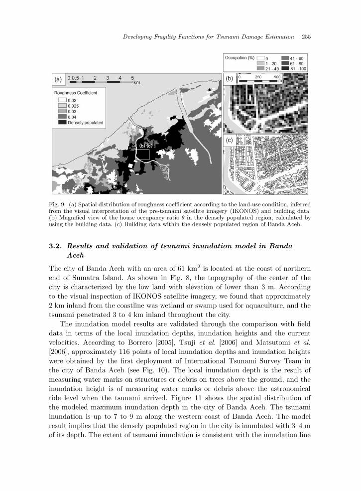
data, and D is the modeled flow depth. Figure 9 shows the spatial distribution of

n0 and θ in the computational domain of tsunami inundation model. n0 is obtained

through the visual interpretation of high-resolution satellite imagery (IKONOS)

acquired on 18 June 2004, and θ is obtained by calculating the building area using

GIS data.

August 13, 2009 14:8 WSPC/101-CEJ 00200


Fig. 9. (a) Spatial distribution of roughness coefficient according to the land-use condition, inferredfrom the visual interpretation of the pre-tsunami satellite imagery (IKONOS) and building data.(b) Magnified view of the house occupancy ratio θ in the densely populated region, calculated byusing the building data. (c) Building data within the densely populated region of Banda Aceh.

3.2. Results and validation of tsunami inundation model in Banda

Aceh

The city of Banda Aceh with an area of 61 km2 is located at the coast of northern

end of Sumatra Island. As shown in Fig. 8, the topography of the center of the

city is characterized by the low land with elevation of lower than 3 m. According

to the visual inspection of IKONOS satellite imagery, we found that approximately

2 km inland from the coastline was wetland or swamp used for aquaculture, and the

tsunami penetrated 3 to 4 km inland throughout the city.

The inundation model results are validated through the comparison with field

data in terms of the local inundation depths, inundation heights and the current

velocities. According to Borrero [2005], Tsuji et al. [2006] and Matsutomi et al.

[2006], approximately 116 points of local inundation depths and inundation heights

were obtained by the first deployment of International Tsunami Survey Team in

the city of Banda Aceh (see Fig. 10). The local inundation depth is the result of

measuring water marks on structures or debris on trees above the ground, and the

inundation height is of measuring water marks or debris above the astronomical

tide level when the tsunami arrived. Figure 11 shows the spatial distribution of

the modeled maximum inundation depth in the city of Banda Aceh. The tsunami

inundation is up to 7 to 9 m along the western coast of Banda Aceh. The model

result implies that the densely populated region in the city is inundated with 3–4 m

of its depth. The extent of tsunami inundation is consistent with the inundation line

August 13, 2009 14:8 WSPC/101-CEJ 00200


Fig. 10. Measured points of the tsunami survey teams; (a) The local inundation depth by Borrero[2005], (b) the inundation height above the astronomical tide level when the tsunami arrived,by Tsuji et al. [2005] and Matsutomi et al. [2006], (c) the definition of field measurements. Themeasured points are indicated by the numbers enumerated by the authors. The solid line is theinundation line interpreted from the post-tsunami satellite imagery (IKONOS) and the field surveyby JICA [2005]. The background gray scale color indicates the land elevation getting higher as thegray scale is darker.

obtained by the visual interpretation of the post-tsunami satellite imagery and field

survey by JICA [2005], approximately 4 km inland from the shore line. The point

to point comparison is shown in Fig. 12, both for the local inundation depth and

inundation height. The model results are, in general, consistent with the measured

August 13, 2009 14:8 WSPC/101-CEJ 00200


Fig. 11. Spatial distribution of modeled inundation depth. The solid line indicates the inundationline.

10

8

6

4

2

0

Modele

d (

m)

1086420

Measured (m)

1

234

5 6

7

89

101112

13

1415

16

17

18

19

20

21

2223

24

2526

2728

29

30

31

32

33

34

35

36

37

3839 40

4142

43

44

45

46

(a) Inundation depth 12

10

8

6

4

2

0

Modele

d (

m)

121086420

Measured (m)

1

3

45

6

78910111213

1415161718192021222324 252627 28293031 3233 343536

37

383940 414243 44

45464748 495051

5253

5455

56

57

585960

61

62 6364

65

66

67

686970

(b) Water level

Fig. 12. Comparison of the model results and the field data, in terms of (a) the local inundationdepths and (b) the inundation heights. The numbers in the plot indicate the measured points inFig. 10.

August 13, 2009 14:8 WSPC/101-CEJ 00200


data, except for several points along the south-western coast. In that area, the model

is underestimated to the measured data, which implies the limitation of the tsunami

inundation model with the shallow water approximation, the possibility that the field

data represents the extreme feature of tsunami shoaling, or lack of local bathymetric

features in the model.

The validation of the model is performed by K and κ proposed by Aida [1978].

Aida’s K and κ are defined as;

log K =1

n

n∑

i=1

log Ki (8)

log κ =

√

√

√

√

1

n

n∑

i=1

(log Ki)2 − (log K)2 (9)

Ki =Ri

Hi(10)

where Ri and Hi are the measured and modeled values of inundation height/depth

at point i. Thus K is defined as the geometrical mean of Ki and κ as deviation or

variance from K, and those indices are used as the criteria to validate the model

through the comparison between the modeled and measured tsunamis.

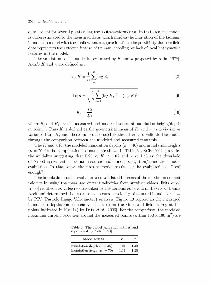
The K and κ for the modeled inundation depths (n = 46) and inundation heights

(n = 70) in the computational domain are shown in Table 3. JSCE [2002] provides

the guideline suggesting that 0.95 < K < 1.05 and κ < 1.45 as the threshold

of “Good agreement” in tsunami source model and propagation/inundation model

evaluation. In that sense, the present model results can be evaluated as “Good

enough”.

The inundation model results are also validated in terms of the maximum current

velocity by using the measured current velocities from survivor videos. Fritz et al.

[2006] rectified two video records taken by the tsunami survivors in the city of Banda

Aceh and determined the instantaneous current velocity of tsunami inundation flow

by PIV (Particle Image Velocimetry) analysis. Figure 13 represents the measured

inundation depths and current velocities (from the video and field survey at the

points indicated in Fig. 14) by Fritz et al. [2006]. For the comparison, the modeled

maximum current velocities around the measured points (within 100 × 100 m2) are

Table 3. The model validation with K andκ proposed by Aida [1978].

Model results K κ

Inundation depth (n = 46) 1.01 1.40

Inundation height (n = 70) 1.11 1.20

August 13, 2009 14:8 WSPC/101-CEJ 00200


5

4

3

2

1

0

Curr

ent velo

city (

m/s

)

543210

Inundation depth (m)

Point A

Point B

Mean value

Maximum and minimum values

Modeled maximum velocity

Fig. 13. Measured flow depths and current velocities from survivor videos, by Fritz et al. [2006],and the modeled current velocities (bars of black solid line). The video was taken at two points;point A is at the grand mosque in the middle of the city and point B at the 2nd-story balcony ofresidential home at the south-west of the city. These two points are indicated in Fig. 14.

shown in the figure. The current velocities of tsunami inundation flow vary from

2 to 4 m/s at point A (Froude number Fr = 0.95 to 1.04 in average), and 3.3 to

4.5 m/s at point B (Fr = 0.61 in average), according to Fritz et al. [2006]. The model

shows slightly underestimated both at point A and B. The spatial distribution of

modeled maximum current velocities are shown in Fig. 14 with the points at which

the velocities were measured. The modeled maximum velocities are obtained as 2 to

3 m/s at point A and 3 to 4 m/s at point B, while the measurements indicate 2 to

4 m/s and 3.3 to 4.5 m/s respectively. We can see that the model result looks good

for calculating local inundation flow except for that in the densely populated region,

although it is not enough to discuss the general validation of the model with only two

measurements. In particular, the observed feature of tsunami inundation at point A

reflects the flow acceleration along the narrow street, which cannot be considered in

the present inundation model using the composite equivalent roughness coefficient.

For the discussion of this sort of significant local features of inundation flow, the

spatial resolution of the model should be increased to at least the same scale of the

houses or streets (several meters) and the higher approximation of the model may be

required (not the 2-dimensional shallow water approximation). On the other hand,

the present model sufficiently provides the accuracy for calculating the inundation

at not-densely populated region as shown in point B.

August 13, 2009 14:8 WSPC/101-CEJ 00200


Fig. 14. Spatial distribution of modeled current velocities and the points at which the velocitieswere measured (see Fig. 13) by the analysis of survivor videos.

August 13, 2009 14:8 WSPC/101-CEJ 00200


4. Developing Fragility Functions

4.1. Methods

Developing the fragility functions for house/structural damage consists of the inte-

gration of three analyses, i.e. numerical analysis, GIS analysis and statistical analy-

sis, as shown in Fig. 15. Also as described in the introduction, the fragility functions

are expressed by the damage probabilities of houses/structures, as the functions

of hydrodynamic features of tsunami inundation flow, such as inundation depths,

current velocities and hydrodynamic forces. To develop the fragility functions, we

take a statistical approach with synergistic use of the numerical model results and

post-tsunami data, as itemized below.

(1) Damage data collection: To obtain the damage data for individual

houses/structures and to develop the inventory of each structure with its ID

number and damage interpretation (destroyed or survived).

(2) Data correlation between the structural damage and tsunami hazard: To corre-

late a table of structure ID, the damage interpretation, and the hydrodynamic

features of tsunami inundation, through the GIS analysis.

Damage data collection Building

damage data set and developing

house inventory, e.g. JICA [2005]

Hazard information Modeling the

hydrodynamic features of tsunami inun-

dation flow.

Calculating the damage probability :

Counting the number of the houses within the

corresponding range of hydrodynamic features

Sample determination : Exploring the range

of hydrodynamic features of tsunami for the

determined sample number and checking the

data distribution

Data correlation between the damage

data and hydrodynamic features of tsunami

Regression analysis : Least-square fitting to

the discrete set of damage probabilities and

hydrodynamic features

GIS Analysis

Statistical Analysis

Numerical Analysis

Fig. 15. The process of developing fragility functions.

August 13, 2009 14:8 WSPC/101-CEJ 00200


(3) Sample determination: Sample sorting by the level of hydrodynamic features, to

explore an arbitrary range of them so that each range includes the determined

number of samples and to check the data distribution.

(4) Calculating damage probability: To calculate the damage probabilities by count-

ing the number of destroyed or survived structures, for each range of hydrody-

namic features described above.

(5) Regression analysis: To develop the fragility function by the regression analysis

of the discrete set of the damage probabilities and hydrodynamic features of

tsunami.

4.2. Post-tsunami survey data

We acquired the post-tsunami survey data from JICA [2005], which was based on

the visual interpretation of the pre and post-tsunami satellite imageries (IKONOS)

with some random field check, focusing on the existence of individual structures’

roofs. Figure 16 indicates the post-tsunami survey result in terms of structural

damage in the city, by JICA [2005]. As shown in the right panels of the figure,

using of high-resolution optical satellite imageries have the capabilities to detect

individual damage and have been utilized as one of the promising technologies for

post-disaster damage investigation. Throughout the visual inspection of two satellite

imageries, the remained roofs were interpreted as “survived” and the disappeared

as “destroyed”.

4.3. Fragility function for structural damage

GIS analysis to integrate both hazard information (Figs. 11 or 14) and damage

interpretation (Fig. 16) leads to an aggregate as shown in the histogram of Fig. 17.

And as a result of calculating the number of destroyed and survived structures

within each inundation depth range, we obtain a relationship between the damage

probability and inundation depth, as shown in Fig. 18. The inundation depth in

the plot of Fig. 18 is determined by taking the median value within a range which

includes approximately 1,000 structures in it.

We can see that the plot shown in Fig. 18 is a discrete set of damage probabilities

of structures and tsunami inundation depths. Then, we explore this relationship

with the form of “fragility function” by performing a linear regression analysis.

From an analogy of earthquake engineering studies, e.g. [Murao and Yamazaki,

2000], [Shinozuka et al., 2002] and [Karim and Yamazaki, 2003], we assume that the

cumulative probability P of occurrence of the damage is given as either Eqs. (11)

or (12).

P (x) = Φ

[

x − µ

σ

]

(11)

August 13, 2009 14:8 WSPC/101-CEJ 00200


Fig. 16. (a) Spatial distribution of structural damage interpreted from the post-tsunami satelliteimagery (IKONOS) by JICA [2005]. Black dots indicate the interpreted structures as “destroyed”,and the gray dots as “survived”. The arrow points the expanded region shown in the right panelsof (b) pre-tsunami, (c) post-tsunami satellite imageries and (d) interpreted damage.

P (x) = Φ

[

lnx − µ′

σ′

]

(12)

where Φ is the standardized normal (lognormal) distribution function, x is the hy-

drodynamic feature of tsunami (e.g. inundation depth, current velocity and hydro-

dynamic force), µ and σ (µ′ and σ′) are the mean and standard deviation of x (ln x)

respectively.

Two statistical parameters of fragility function, i.e. µ and σ (µ′ and σ′), are ob-

tained by plotting x (lnx) and the inverse of Φ−1 on normal or lognormal probability

papers, and performing the least-squares fitting of this plot, as shown in Fig. 19.

Hence, two parameters are obtained by taking the intercept (= µ or µ′) and the

angular coefficient (= σ or σ′) in Eqs. (13) or (14);

x = σΦ−1 + µ (13)

lnx = σ′Φ−1 + µ′ (14)

Throughout the regression analysis, the parameters are determined as shown in

Table 4, to obtain the best fit of fragility functions with respect to the inundation

August 13, 2009 14:8 WSPC/101-CEJ 00200


0

200

400

600

800

1000

1200

0.2

0.4

0.6

0.8

1.0

1.2

1.3

1.5

1.7

1.9

2.1

2.2

2.4

2.6

2.8

2.9

3.1

3.3

3.5

3.7

3.9

4.0

4.2

4.3

4.5

4.7

4.8

5.0

5.1

5.3

5.6

6.7

8.2

Inundation depth (< x m)

Destroyed

Survived

Number of

Fig. 17. Histogram of the numbers of destroyed and survived structures in terms of inundationdepth range, within the tsunami inundation zone. Each inundation depth range is determined byexploring a range which includes approximately 1,000 structures.

1.0

0.8

0.6

0.4

0.2

Da

ma

ge

pro

ba

bili

ty

86420


Fig. 18. The plot of damage probabilities and the median values of inundation depths that werecompiled from sample data.

August 13, 2009 14:8 WSPC/101-CEJ 00200


6

5

4

3

2

1

0

Inu

nd

atio

n d

ep

th (

m)

-3 -2 -1 0 1 2 3

Φ−1

Least-squares fit

Fig. 19. An example of the plot on normal probability paper.

Table 4. Parameters for fragility functions obtained through the regression analy-sis. R2 is the coefficient of determination obtained through the least-squares fitting.

x for fragility functions P (x) µ σ µ′ σ′ R2

Inundation depth (m) 2.99 1.12 N/A N/A 0.99

Current velocity (m/s) N/A N/A 0.80 0.28 0.97

Hydrodynamic force per width (kN/m) N/A N/A 1.47 0.75 0.99

depth (m), the maximum current velocity (m/s) and the hydrodynamic force on

structures per unit width (kN/m). Here the hydrodynamic force acting on a structure

is defined as the drag force per unit width of it;

F =1

2CDρu2D (15)

where CD is the drag coefficient (CD = 1.0 for simplicity), ρ is the density of water

(= 1,000 kg/m3), u is the current velocity (m/s), and D is the inundation depth (m).

Note that the fragility function with respect to the inundation depth is given by the

standardized normal distribution function with µ and σ, while those with respect

to the current velocity and hydrodynamic force are by the standardized lognormal

distribution functions with µ′ and σ′.

As a result, the fragility functions (fragility curves) are obtained as Fig. 20, indi-

cating the damage probabilities according to the hydrodynamic features of tsunami

inundation flow in Banda Aceh. For instance, we can see that the structures were

significantly vulnerable when the local inundation depth exceeds 2 or 3 m, the cur-

rent velocity exceeds 2.5 m/s or hydrodynamic load on a structure exceeds 5 kN/m.

However, note that the observed structural damage in the site might consist of both

August 13, 2009 14:8 WSPC/101-CEJ 00200


��

��

��

��

��

��

��

��! #"!�%$ &�')( *,+.-0/21)3

465 7

7#5 8

7#5 9

7#5 :

7#5 ;

7#5 7

< =>=?@ABCD =DEFE G H

89:;7I J#K�J!L�M�N�O P�JQL�R�STN�U,V.WYX

Z6[ \

\#[ ]

\#[ ^

\#[ _

\#[ `

\#[ \

a bcbdefghi bijkj l m

_!\no\`!\Zp\\qsr)tvu�w�t�r#x)y�zY{ |~}2w�u�|T��.�T�s�.z,�

Fig. 20. Fragility functions (fragility curves) for building damage, in terms of the inundation depth,the current velocity and the hydrodynamic force obtained from the numerical model. The solidlines are the best-fitted curves of the plot (◦: the distribution of damage probabilities) with theparameters in Table 4.

damage by tsunami and strong ground motion. In fact, the major structure types in

the tsunami-affected area were low-rise wooden house, timber construction, and non-

engineered RC construction which is lightly reinforced, and it was reported that the

large number of the houses and structures survived the strong ground motion with

minor damage on walls then destroyed by the tsunami, e.g. [Saatcioglu et al., 2006].

Since the damage interpretation using the pre and post-tsunami satellite imageries

focuses on if the houses’ roofs were remained or not, we supposed that the structural

damage was caused by the tsunami inundation. Also, note that the tsunami damage

on structures were caused by both hydrodynamic force/impact and the impact of

floating debris, i.e. these facts are reflected on the damage probabilities but not on

the numerical model results (the estimated hydrodynamic features). In that sense,

the present fragility functions might indicate overestimation in terms of the damage

probabilities to the hydrodynamic features of tsunami inundation flow.

August 13, 2009 14:8 WSPC/101-CEJ 00200


In the practical issues, the fragility functions can be used for structural damage

estimation, combined with the tsunami inundation models. In that use, the authors

recommend to apply the fragility function with regard to the inundation depth. The

reason for this is that the estimation of current velocity is significantly affected by

the grid resolution and its accuracy of topography data used, the resistance low

applied, and also the approximation of the model itself. Even if the state-of-the-art

technologies in the computational fluid dynamics (CFD) models are performed, the

estimation of local tsunami current velocity, especially of the inundation flow among

the densely populated area, is one of the significant problems.

4.4. Fragility function for tsunami casualty

Also, the fragility function for tsunami casualty is determined by using the post-

tsunami data in terms of the number of dead and survived residents. Figure 21 is the

spatial distribution of the ratio of dead, missing and survived people in each Desa

(village) of Banda Aceh city, normalized by the pre-tsunami population in each Desa

(The data was compiled by JICA [2005]).

GIS analysis of the casualty information and the numerical model results shown

in Fig. 14 leads to the fragility function for tsunami casualties described as the re-

lationship between the death ratio (both dead and missing) and the hydrodynamic

features of tsunami. According to the data of tsunami casualties in Fig. 21, the

representative value of local hydrodynamic feature of tsunami inundation is calcu-

lated by taking the median value of modeled inundation depths within each Desa.

Figure 22 shows the variation and standard deviation of the local inundation depths

within each Desa, obtained by GIS analysis using the numerical model results. We

can see, from the figure, that the inundation depths within each Desa are highly

dispersed.

Figure 23 shows the fragility function expressed as the death ratio with regard to

the representative value of inundation depth calculated by taking the median value

of the numerical model results within each Desa (see Fig. 22). The fragility function

is determined by assuming the standardized normal distribution function, as shown

in Eq. (16) with the parameters µ = 3.75, σ = 1.35, and R2 = 0.80 obtained through

the least-squares fitting;

P (x) = Φ

[

x − 3.75

1.35

]

(16)

where x is the median value of the inundation depth (m) in each Desa, calculated

by using the numerical model results.

Note that the death ratio distribution of Fig. 21 is the result of the post-tsunami

investigation based on the pre-tsunami registration data. It is highly unknown ex-

actly where the residents were affected by the tsunami inundation flow, because it is

easily guessed that the residents who were aware of tsunami arrival have evacuated

August 13, 2009 14:8 WSPC/101-CEJ 00200


Desa boundary

Population ratio

Saved

Missing

Dead

0.5

0 1 2 3 4 50.5km

0 10 205km

Inundation limit

0

43

2

1

8

5

976

10

20

11

14

33

12

48

23

81

31

15

85

29

51

82

17

30

6664

60

16

75 76

79

13 1819

8083

39

59

50

35

71

4753

69 68

78

5242

72

62

26

41

37

67

86

4540

88

6155

2236

25

34

5456

65

77

49

57

32

70

84

44

87

63

28

74

43

21

73

38

46

27

58

24

(b)

( )

Desa boundaryx

Desa index

Fig. 21. (a) Death/Surviving ratio for each Desa (Village), compiled by JICA [2005], and (b) Desaindex for Fig. 22.

August 13, 2009 14:8 WSPC/101-CEJ 00200


8

6

4

2

0

Inundation d

epth

(m

)

806040200

Median

Mean

1.5

1.0

0.5

0.0

Sta

ndard

devia

tion

806040200

(a)

(b)

Maximum

Minimum

5000

4000

3000

2000

1000

0

Num

ber

of sam

ple

s

806040200

Desa index

(c)

Fig. 22. (a) Variation and (b) standard deviation of the local inundation depths within each Desa,calculated by GIS analysis using the numerical model results. (c) Number of samples (computationalgrids) included in each Desa. The horizontal axis (Desa index) corresponds to Fig. 21(b).

and tried to survive. In other words, the fragility curve of Fig. 23 does not indi-

cate the human’s survival possibility according to the local hydrodynamic features

of tsunami inundation flow, e.g. [Koshimura et al., 2006]. Also, taking the median

value to obtain the representative of tsunami inundation depth according to each

Desa reflects the higher dispersion of the plot compared with that of Fig. 20. For the

above reasons, this fragility function should be interpreted as a macroscopic mea-

sure of tsunami impact, i.e. the potential tsunami casualties increase when tsunami

inundation depth exceeds 2 m and almost no survivor is expected when it is 8 m.

5. Concluding Remarks

Using the high-resolution bathymetry and topography data, we performed a tsunami

inundation modeling for the 2004 Sumatra–Andaman earthquake tsunami that

August 13, 2009 14:8 WSPC/101-CEJ 00200


1.0

0.8

0.6

0.4

0.2

0.0

Death

ratio

86420


Fig. 23. Fragility function for tsunami casualty in terms of the inundation depth. The solid line isthe best-fitted curve of the plot (◦: the distribution of death rate) with Eq. (16).

attacked the city of Banda Aceh. The model results in terms of the local inundation

depth: the extent of inundation zone where the current velocity are consistent with

the actually measured and interpreted data from satellite imagery.

Combined use of the numerical model results and GIS analysis, using the post-

tsunami survey data in terms of the damage on structures and casualties, thus

developing the fragility functions to assess Banda Aceh’s vulnerability against the

2004 tsunami. The fragility functions are expressed by the damage probabilities of

houses/structures and death rate in terms of the hydrodynamic features of tsunami

inundation flow such as local inundation depth, current velocity and hydrodynamic

force. As a consequence of developing fragility functions, they lead to the new un-

derstandings of the local tsunami impact in a quantitative manner, the relationship

between local vulnerability and tsunami hazard.

Also, the fragility functions that we proposed can be used as a measure to assess

the damage due to the potential tsunami. The potential damage on structures or

casualties due to the variety of tsunami scenarios can be estimated by multiply-

ing the number of tsunami exposure (e.g. houses and populations) by the fragility

functions (damage probabilities) according to the local features of tsunami obtained

by tsunami inundation models such as [Borrero et al., 2006]. However, note that

the fragility functions in the present study are from the event which occurred in

Banda Aceh, and they do not imply the universal measure of tsunami impact or

damage. As described above, vulnerabilities should include the multitude of uncer-

tain sources, such as hydrodynamic features of tsunami inundation flow, structural

August 13, 2009 14:8 WSPC/101-CEJ 00200


characteristics and site conditions. In other words, they may not be applicable for

considering tsunami vulnerabilities in other areas or tsunami scenarios. Thus, care-

ful use is required when users apply the present fragility functions on their tsunami

damage estimation studies in the other areas or countries.

Acknowledgments

The authors sincerely thank Japan International Cooperation Agency (JICA) and all

the researchers, especially of Syiah Kuala University, working on the 2004 Sumatra–

Andaman earthquake tsunami for providing the post-tsunami survey data. This

research was supported by the Industrial Technology Research Grant Program in

2008 (Project ID: 08E52010a) from New Energy and Industrial Technology Develop-

ment Organization (NEDO), and the Grant-in-Aid for Scientific Research (Project

Number: 19681019 and 18201033) from the Ministry of Education, Culture, Sports,

Science and Technology (MEXT).

References

Aburaya, T. & Imamura, F. [2002] “The proposal of a tsunami run-up simulation using com-bined equivalent roughness,” Annual Journal of Coastal Engineering, JSCE 49, 276–280 (inJapanese).

Aida, I. [1978] “Reliability of a tsunami source model derived from fault parameters,” Journal ofPhysics of the Earth 26, 57–73.

Ammon, C. J., Ji, C., Thio, H. K., Robinson, D., Ni, S., Hjorleifsdottir, V., Kanamori, H., Lay, T.,Das, S., Helmberger, D., Ichinose, G., Polet, J. & Wald, D. [2005] “Rupture process of the2004 Sumatra–Andaman earthquake,” Science 308, 1133–1139.

Borrero, J. [2005] “Field survey of northern Sumatra and Banda Aceh, Indonesia after the tsunamiand earthquake of 26 December 2004,” Seismological Research Letters 76(3), 309–318.

Borrero, J., Sieh, K., Chlieh, M. & Synolakis, C. E. [2006] “Tsunami inundation modeling forwestern Sumatra,” Proc. National Academy of Science, 103(52), 19673–19677.

British Oceanographic Data Centre [1997] “The Centenary Edition of the GEBCO Digital Atlas(CD-ROM).”

Chlieh, M., Avouac, J., Hjorleifsdottir, V., Song, T. A., Ji, C., Sieh, K., Sladen, A., Herbert, H.,Prawirodirdjo, L., Bock, Y. & Galetzka, J. [2007] “Coseismic slip and afterslip of the greatMw 9.15 Sumatra–Andaman earthquake of 2004,” Bulletin of the Seismological Society ofAmerica 97(1A), S152–S173.

Dasgupta, S., Mukhopadhyay, M., Bhattacharya, A. & Jana, T. K. [2003] “The geometry of theBurmese–Andaman subducting lithosphere,” Journal of Seismology 7, 155–174.

Dutta, D., Alam, J., Umeda, K., Hayashi, M. & Hironaka, S. [2007] “A two-dimensional hydrody-namic model for flood inundation simulation: A case study in the lower Mekong river basin,”Hydrological Processes 21, 1223–1237.

Federal Emergency Management Agency (FEMA) [2003] Coastal Construction Manual (CCM), 3rdedn. (fema 55), 296p.

Fritz, H. M., Borrero, J. C., Synolakis, C. E. & Yoo, J. [2006] “2004 Indian Ocean tsunami flowvelocity measurements from survivor videos,” Geophysical Research Letters 33, L24605.

Fujii, Y. & Satake, K. [2007] “Tsunami source of the 2004 Sumatra–Andaman earthquake inferredfrom tide gauge and satellite data,” Bulletin of the Seismological Society of America 97(1A),S192–S207.

August 13, 2009 14:8 WSPC/101-CEJ 00200


Fujima, K., Shigihara, Y., Tomita, T., Honda, K., Nobuoka, H., Hanzawa, M., Fujii, H., Otani,H., Orishimo, S., Tatsumi, M. & Koshimura, S. [2006] “Survey results of the Indian Oceantsunami in the Maldives,” Coastal Engineering Journal 48(2), 91–97.

Gower, J. [2007] “The 26 December 2004 tsunami measured by satellite altimetry,” InternationalJournal of Remote Sensing 28(13–14), 2897–2913.

Hayashi, Y. [2007] “Extracting the 2004 Indian Ocean tsunami signals from sea surface heightdata observed by satellite altimetry,” Journal of Geophysical Research 113, C01001,doi:10.1029/2007JC004177.

Hirata, K., Satake, K., Tanioka, Y., Kuragano, T., Hasegawa, Y., Hayashi, Y. & Hamada, N.[2006] “The 2004 Indian Ocean tsunami: Tsunami source model from satellite altimetry,Earth Planets Space 58, 195–201.

Imamura, F. [1995] “Review of tsunami simulation with a finite difference method,” Long-WaveRunup Models (World Scientific), pp. 25–42.

Ishii, M., Shearer, P. M., Houston, H. & Vidale, J. E. [2005] “Extent, duration and speed of the2004 Sumatra–Andaman earthquake imaged by Hi–Net array,” Nature 435, 933–936.

Japan International cooperation Agency (JICA) [2005] “The study on the urgent rehabilitationand reconstruction support program for Aceh province and affected areas in north Sumatra,”Final Report (1), Vol. IV: Data book.

Japan Society of Civil Engineers [2002] “Tsunami assessment method for nuclear power plants inJapan,” 72p.

Karim, K. R. & Yamazaki, F. [2003] “A simplified method of constructing fragility curves forhighway bridges,” Earthquake Engineering and Structural Dynamics 32, 1603–1626.

Koshimura, S., Katada, T., Mofjeld, H. O. & Kawata, Y. [2006] “A method for estimating casualtiesdue to the tsunami inundation flow,” Natural Hazards 39, 265–274.

Kotani, M., Imamura, F. & Shuto, N. [1998] “Tsunami run-up simulation and damage estimationby using geographical information system,” Proc. Coastal Engineering, JSCE 45, 356–360 (inJapanese).

Lay, T., Kanamori, H., Ammon, C. J., Nettles, M., Ward, S. N., Aster, R. C., Beck, S. L., Bilek,S. L., Brudzinski, M. R., Butler, R., DeShon, H. R., Ekstrom, G., Satake, K. & Sipkin, S.A. [2005] “The great Sumatra–Andaman earthquake of 26 December 2004,” Science 308,1127–1133.

Mansinha, L. & Smylie, D. E. [1971] “The displacement fields of inclined faults,” Bulletin of theSeismological Society of America 61(5), 1433–1440.

Matsutomi, H., Sakakiyama, T., Nugroho, S. & Matsuyama, M. [2006] “Aspects of inundated flowdue to the 2004 Indian Ocean tsunami,” Coastal Engineering Journal 48(2), 167–195.

Miura, H., Wijeyewickrema, A. & Inoue, S. [2006] “Evaluation of tsunami damage in the easternpart of Sri Lanka due to the 2004 Sumatra earthquake using remote sensing technique,” inProc. 8th National Conference on Earthquake Engineering, Paper No. 8, NCEE-856.

Murao, O. & Yamazaki, F. [2000] “Development of fragility curves for buildings based on damagesurvey data of a local government after the 1995 Hyogoken–Nanbu earthquake, Journal ofStructural and Construction Engineering 527, 189–196 (in Japanese).

Nagano, O., Imamura, F. & Shuto, N. [1991] “A numerical model for far-field tsunamis and itsapplication to predict damages done to aquaculture,” Natural Hazards 4, 235–255.

Oie, T., Koshimura, S., Yanagisawa, H. & Imamura, F. “Numerical modeling of the 2004 IndianOcean tsunami and damage assessment in Banda Aceh, Indonesia,” Annual Journal of CoastalEngineering, JSCE 53, 221–225 (in Japanese).

Piatanesi, A. & Lorito, S. [2007] “Rupture process of the 2004 Sumatra–Andaman earthquakefrom tsunami waveform inversion,” Bulletin of the Seismological Society of America 97(1A),S223–S231.

Rabus, B., Eineder, M., Roth, A. & Bamler, R. [2003] “The shuttle radar topography mission —a new class of digital elevation models acquired by spaceborne radar,” Photogramm. Rem.Sens. 57, 241–262.

August 13, 2009 14:8 WSPC/101-CEJ 00200


Rajendran, C. P., Rajendran, K., Anu, R., Earnest, A., Machado, T., Mohan, P. M. & Freymueller,J. [2007] “Crustal deformation and seismic history associated with the 2004 Indian Oceanearthquake: A Perspective from the Andaman–Nicobar Islands,” Bulletin of the SeismologicalSociety of America 97(1A), S174–S191.

Saatcioglu, M., Ghobarah, A. & Nistor, I. [2006] “Performance of structures in Indonesia during theDecember 2004 great Sumatra earthquake and Indian Ocean tsunami,” Earthquake Spectra22(3), S295–S319.

Satake, K., Aung, T. T., Sawai, Y., Okamura, Y., Win, K. S., Swe, W., Swe, C., Swe, T. L.,Tun, S. T., Soe, M. M., Oo, T. Z. & Zaw, S. H. [2006] “Tsunami heights and damage alongthe Myanmar coast from the December 2004 Sumatra–Andaman earthquake,” Earth PlanetsSpace 58, 243–252.

Shigihara, Y. & Fujima, K. [2006] “Dispersion effects in the Indian Ocean tsunami,” Annual Journalof Coastal Engineering, JSCE 53, 266–270 (in Japanese).

Shinozuka, M., Feng, M. Q., Lee, J. & Naganuma, T. “Statistical analysis of fragility curves,”Journal of Engineering Mechanics 126(12), 1224–1231.

Shuto, N. [1993] “Tsunami intensity and disasters,” Tsunamis in the World (Kluwer AcademicPublishers), pp. 197–216.

Sieh, K. [2007] “The Sunda Megathrust — Past, present and future,” Journal of Earthquake andTsunami 1(1), 1–19.

Tanioka, Y., Yudhicara, Kusunose, T., Kathiroli, S., Nishimura, Y., Iwasaki, S. & Satake, K. [2006]“Rupture process of the 2004 great Sumatra–Andaman earthquake estimated from tsunamiwaveforms, Earth Planets Space 58, 203–209.

Tobita, M., Suito, H., Imaikire, T., Kato, M., Fujiwara, S. & Murakami, M. [2006] “Outline ofvertical displacement of the 2004 and 2005 Sumatra earthquakes revealed by satellite radarimagery,” Earth Planets Space 58, e1–e4.

Tomita, T., Imamura, F., Arikawa, T., Yasuda, T. & Kawata, Y. [2006] “Damage caused by the 2004Indian Ocean tsunami on the southwester coast of Sri Lanka,” Coastal Engineering Journal48(2), 99–116.

Tsuji, Y., Tanioka, Y., Matsutomi, H., Nishimura, Y., Kamataki, T., Murakami, Y., Sakakiyama, T.,Moore, A., Gelfenbaum, G., Nuguroho, S., Waluyo, B., Sukanta, I., Triyono, R. & Namegaya,Y. [2006] “Damage and height distribution of Sumatra earthquake–Tsunami of December 26,2004, in Banda Aceh city and its environs,” Journal of Disaster Research 1(1), 103–115.

U.S. Geological Survey (USGS), Earthquake Hazard Program, http://earthquake.usgs.gov/.Yamamoto, Y., Takanashi, H., Hettiarachchi, S. & Samarawickrama, S. [2006] “Verification of the

destruction mechanism of structures in Sri Lanka and Thailand due to the Indian Oceantsunami,” Coastal Engineering Journal 48(2), 117–145.

Vu, T. T., Matsuoka, M. & Yamazaki, F. [2007] “Dual–scale approach for detection of tsunami-affected areas using optical satellite images,” International Journal of Remote Sensing 28(13–14), 2995–3011.

DEVELOPING FRAGILITY FUNCTIONS FOR … within the city of Banda Aceh, using high-resolution...

Documents

Transcript of DEVELOPING FRAGILITY FUNCTIONS FOR … within the city of Banda Aceh, using high-resolution...