Judy Busby, Doug Sondak, Brent Staubach, and Roger DavisUnited Technologies Research Center,Pratt & Whitney, East Hartford, Connecticut

Deterministic Stress Modeling ofHot Gas Segregation in a Turbine

NASA/CR—1998-208666

October 1998

UTRC Report 98–07

https://ntrs.nasa.gov/search.jsp?R=19980237200 2018-06-05T19:45:27+00:00Z

The NASA STI Program Office . . . in Profile

Since its founding, NASA has been dedicated tothe advancement of aeronautics and spacescience. The NASA Scientific and TechnicalInformation (STI) Program Office plays a key partin helping NASA maintain this important role.

The NASA STI Program Office is operated byLangley Research Center, the Lead Center forNASA’s scientific and technical information. TheNASA STI Program Office provides access to theNASA STI Database, the largest collection ofaeronautical and space science STI in the world.The Program Office is also NASA’s institutionalmechanism for disseminating the results of itsresearch and development activities. These resultsare published by NASA in the NASA STI ReportSeries, which includes the following report types:

• TECHNICAL PUBLICATION. Reports ofcompleted research or a major significantphase of research that present the results ofNASA programs and include extensive dataor theoretical analysis. Includes compilationsof significant scientific and technical data andinformation deemed to be of continuingreference value. NASA’s counterpart of peer-reviewed formal professional papers buthas less stringent limitations on manuscriptlength and extent of graphic presentations.

• TECHNICAL MEMORANDUM. Scientificand technical findings that are preliminary orof specialized interest, e.g., quick releasereports, working papers, and bibliographiesthat contain minimal annotation. Does notcontain extensive analysis.

• CONTRACTOR REPORT. Scientific andtechnical findings by NASA-sponsoredcontractors and grantees.

• CONFERENCE PUBLICATION. Collectedpapers from scientific and technicalconferences, symposia, seminars, or othermeetings sponsored or cosponsored byNASA.

• SPECIAL PUBLICATION. Scientific,technical, or historical information fromNASA programs, projects, and missions,often concerned with subjects havingsubstantial public interest.

• TECHNICAL TRANSLATION. English-language translations of foreign scientificand technical material pertinent to NASA’smission.

Specialized services that complement the STIProgram Office’s diverse offerings includecreating custom thesauri, building customizeddata bases, organizing and publishing researchresults . . . even providing videos.

For more information about the NASA STIProgram Office, see the following:

• Access the NASA STI Program Home Pageat http://www.sti.nasa.gov

• E-mail your question via the Internet tohelp@sti.nasa.gov

• Fax your question to the NASA AccessHelp Desk at (301) 621-0134

• Telephone the NASA Access Help Desk at(301) 621-0390

• Write to: NASA Access Help Desk NASA Center for AeroSpace Information 7121 Standard Drive Hanover, MD 21076

Judy Busby, Doug Sondak, Brent Staubach, and Roger DavisUnited Technologies Research Center,Pratt & Whitney, East Hartford, Connecticut

Deterministic Stress Modeling ofHot Gas Segregation in a Turbine

NASA/CR—1998-208666

October 1998

National Aeronautics andSpace Administration

Lewis Research Center

Prepared under Contract NAS3–26618Task Order 28

UTRC Report 98–07

Acknowledgments

Available from

NASA Center for Aerospace Information7121 Standard DriveHanover, MD 21076Price Code: A03

National Technical Information Service5285 Port Royal RoadSpringfield, VA 22100

Price Code: A03

This work was performed with support from NASA Lewis Research Center and funded by theHigh Performance Computing and Communication Program (HPCCP). The authors appreciate the

guidance and support of the NASA Lewis technical monitor, Mr. Joseph Veres. In addition, the authors wouldlike to acknowledge the technical support of Dr. Om Sharma and Dr. Ron-Ho Ni of Pratt & Whitney.

Finally, the second author in this effort, Dr. Doug Sondak, is now located at Boston Universityin the Office of Information Technology.

NASA/CR—1998-208666 1

DETERMINISTIC STRESS MODELING OF HOT GASSEGREGATION IN A TURBINE

Judy Busby, Doug Sondak, Brent Staubach, and Roger DavisUnited Technologies Research Center

and Pratt and WhitneyEast Hartford, Connecticut 06108

AbstractSimulation of unsteady viscous turbomachinery flowfields is presently

impractical as a design tool due to the long run times required. Designers relypredominantly on steady-state simulations, but these simulations do not accountfor some of the important unsteady flow physics. Unsteady flow effects can bemodeled as source terms in the steady flow equations. These source terms,referred to as Lumped Deterministic Stresses (LDS), can be used to drive steadyflow solution procedures to reproduce the time-average of an unsteady flowsolution. The goal of this work is to investigate the feasibility of using inviscidlumped deterministic stresses to model unsteady combustion hot streakmigration effects on the turbine blade tip and outer air seal heat loads using asteady computational approach. The LDS model is obtained from an unsteadyinviscid calculation. The LDS model is then used with a steady viscouscomputation to simulate the time-averaged viscous solution.

Both two-dimensional and three-dimensional applications are examined.The inviscid LDS model produces good results for the two-dimensional case andrequires less than 10% of the CPU time of the unsteady viscous run. For thethree-dimensional case, the LDS model does a good job of reproducing the time-averaged viscous temperature migration and separation as well as heat load onthe outer air seal at a CPU cost that is 25% of that of an unsteady viscouscomputation.

IntroductionExperimental data taken from gas turbine combustors indicates that the flow

exiting the combustor has both circumferential and radial temperature gradients.These temperature gradients have significant impact on the wall temperature ofthe first stage rotor. A combustor hot streak, which can typically havetemperatures twice the free stream stagnation temperature, has a greaterstreamwise velocity and cross-flow vorticity than the surrounding fluid andtherefore a larger positive incidence angle to the rotor as compared to the freestream. Due to this rotor incidence variation through the hot streak and the slowconvection speed on the pressure side of the rotor, the hot streak typicallyaccumulates on the rotor pressure surface. As a result, the time-averaged rotor-relative stagnation temperature is larger on the pressure surface than on thesuction side. The secondary flow in the rotor passage also causes the hot fluid

NASA/CR—1998-208666 2

on the pressure side to spread from midspan towards the hub and tip endwalls,resulting in the heating of the outer air seal.

In the absence of total pressure non-uniformities, the temperature gradientsdue to the hot streak have minimal impact on the pressure distribution in therotor. Thus, steady-state computations are typically used to compute thepressure distribution through the first stage of the turbine. For a steady-statecomputation, the tangential components of the hot streak at the exit of the statorare flux-averaged and only the radial variation in the rotor frame is retained.Many authors have shown that the tangential variations in the hot streak are ofprime importance in establishing the hot streak migration path through the bladepassage [1,2,3,4]. By mixing out the tangential variation at the rotor inlet, thesteady-state computations do not model the temperature segregation in theblade passage or produce the correct temperature distributions on the bladesurface.

Previously, the only way to correctly model the hot streak migration throughthe rotor was with three-dimensional time-accurate viscous computations.However, three-dimensional unsteady viscous computations are toocomputationally intensive and time consuming to be integrated into the designprocess. A more desirable approach is to include the time-averaged unsteadyeffects into a steady computation via an unsteady model. For this work, thelumped deterministic stresses associated with an unsteady inviscid calculationare used to model the time-averaged unsteady effects in a steady viscouscalculation. Although unsteady inviscid calculations are more computationallyexpensive than steady inviscid or viscous computations, they require significantlyless computational resources than unsteady viscous computations. Since themigration and segregation of the hot streak in the rotor is predominantlyconvective in nature, the inviscid LDS field should provide a reasonable modelfor the time-averaged temperature distribution in the rotor passage. The inviscidLDS models may also provide insight into the development of an analyticalmodel for the unsteady effects.

Both two-dimensional and three-dimensional LDS models are examined inthis report. For the two-dimensional application, the LDS model is computedfrom a 1-1/2 stage turbine unsteady inviscid hot streak migration calculation.The corresponding LDS field is first applied to a steady inviscid computation as acheck of the overall procedure. Next, the inviscid LDS field is interpolated onto atwo-dimensional viscous grid and a steady viscous solution (with the LDS model)is computed. The inviscid LDS model with the steady viscous solution did agood job of reproducing the viscous time-averaged values of the temperaturesegregation in the passage and the surface temperature distribution on theblade.

Next, the two-dimensional LDS model is extended to three dimensions. Inphase II of this effort, numerous three-dimensional computations for inviscid andviscous steady and unsteady conditions were performed using a strip-blade-stripconfiguration. For the strip-blade-strip configuration, the first and second vaneswere replaced with a narrow (in the axial direction) grid strip. The freestreamboundary conditions on these strips were set with the corresponding first vane

NASA/CR—1998-208666 3

exit and second vane inlet conditions. Along with the strip models, various otherphysical models were used to simulate viscous effects, cooling effects and tipleakage effects. It was determined, however, that these additional physicalmodels produced unrealistic LDS fields and the interaction between the physicaland LDS models needs to be investigated further. Therefore, the additionalphysical models were removed to demonstrate the LDS model by itself and theflow through the stage was recomputed using a vane-blade configuration.

Computational ModelSince deterministic stresses are analogous to turbulent stresses,

decomposing velocities into mean and fluctuating components and applying thedecomposed velocities to the Navier-Stokes equations is a natural starting pointfor modeling the deterministic stresses. Consider the 2-D Navier-Stokesequations:

∂∂

∂∂

∂∂

∂∂

∂∂

Q

t

E

x

F

y

E

x

F

yv v+ + − +

=−Re 1 0 (1)

where Q is the vector of conserved variables, E and F are the convection fluxes,and the diffusion fluxes, Ev and Fv , are given by

E

e

F

f

v

xx

xy

u

v

xy

yy

v

=

=

0 0

5 5

ττ

ττ (2)

wheree u v qu

xx xy x5 = + +τ τ (3)

f u v qvxy yy y5 = + +τ τ (4)

In conventional Reynolds decompositions, velocities are decomposed intomean and fluctuating components, and the stresses τij in the above equations

represent the sum of molecular stresses and turbulent stresses. In the theory ofdeterministic stresses [5], the velocity fluctuations are considered to have arandom (turbulent) component and a deterministic component. Thedeterministic fluctuations occur on larger space and time scales than the randomfluctuations, and are a result of phenomena such as wake passing and rotor-stator potential interaction. In Ref. [5], the flowfield is further decomposed intoan “average passage” and deviations from the average passage, but theaverage-passage analysis is not employed in the present study.

NASA/CR—1998-208666 4

The velocity is first decomposed into a “deterministic” velocity u and astochastic fluctuation ′u ,

u u uj j j= + ′ (5)

The deterministic velocity is further decomposed into a mean value and adeterministic fluctuation,

u u uj j j= + ′′ (6)

This decomposition is illustrated in Fig. 1. The value of is constant, since it isaveraged over all time scales. The smooth curve represents temporal variationof the deterministic velocity , which has a relatively large time scale, and thejagged line represents the instantaneous velocity, u .

The decompositions in Eqns. (5) and (6) may be interpreted as using mass-weighted averaging (Favre averaging) or Reynolds averaging. Here, theNavier-Stokes equations are mass-averaged in the conventional manner usingEqn. (5). The velocity is then further decomposed according to Eqn. (6), and theresulting equation is Reynolds averaged. A combination of mass-weightedaveraging and Reynolds averaging is employed because this yields a moreconvenient form of the equations as compared with using either averagingtechnique alone. These averaging procedures yield two “additional” stressterms,

R u u u uij i j i j= ′ ′ + ′′ ′′ρ ρ (7)

where the first term on the right hand side is the conventional Reynolds stressand the second term on the right hand side is the deterministic stress. The totalstress, τij , therefore has three components: the molecular stress, the turbulent

stress and the deterministic stress.

τ τ τ τij ijm

ijt

ijd= + + (8)

Analogous decomposition is also applicable to the heat transfer rate, qi .Each diffusion flux in Eqn. (2) can be decomposed into three components in

accordance with Eqn. (8). Rewriting Eqn. (1) with this decomposition andexplicitly indicating the functional dependence of the fluxes on Q, yields

[ ] [ ]

∂∂

∂∂

∂∂

∂∂

∂∂

Q

t

E Q

x

F Q

y

xE Q E Q E Q

yF Q F Q F Qv

mvt

vd

vm

vt

vd

+ +

− + + + + +

=−

( ) ( )

Re ( ) ( ) ( ) ( ) ( ) ( )1 0

(9)

NASA/CR—1998-208666 5

Now, define an operator R Q( )

[ ] [ ]R QE Q

x

F Q

y xE Q E Q

yF Q F Qv

mvt

vm

vt( )

( ) ( )Re ( ) ( ) ( ) ( )≡ + − + + +

−∂∂

∂∂

∂∂

∂∂

1 (10)

Note that this operator does not include the time term or the deterministic stressterms. The sum of the deterministic stress terms in both coordinate directions,D , is defined as

D QE Q

x

F Q

yvd

vd

( ) Re( ) ( )

≡ − +

−1 ∂

∂∂

∂ (11)

Applying Eqns. (10) and (11) to Eqn. (9) yields

∂∂Q

tR Q D Q+ + =( ) ( ) 0 (12)

Let Qs represent a steady-state solution (without deterministic stresses), and letQta represent the time-average of an unsteady solution. Since the numericalapproximation of R Q( ) is driven toward zero for a steady-state solution,

R Qs( ) = 0

The time-average of an unsteady solution will not be identical (in general) to thesteady-state solution due to the existence of the deterministic stresses.Averaging a periodic flow over one period results in ∂ ∂Q tta = 0 and thedeterministic stress term, D , is given by

D Q R Qta ta( ) ( )= −

Since the “residual” of the Navier-Stokes solver is the numerical approximationof R Q( ) , one method of computing D Qta( ) is to initialize the flow solver with Qta

and to compute the residual. This, of course, is not a practical method fordeducing the deterministic stresses, since the goal is to solve for Qta withoutincurring the expense of an unsteady computation, but it is a convenient methodfor extracting the D field as an aid toward developing a useful model for D . IfD could be successfully modeled, it could be input to the solver as a sourceterm and convergence to a steady state would then result in the solution for Qta

without performing an unsteady simulation.Some unsteady effects are inviscid, such as vane-blade potential interaction,

and other unsteady effects are viscous, such as wake shedding. A method forcomputing the LDS model without performing an unsteady, viscous simulation is

NASA/CR—1998-208666 6

to use an unsteady, inviscid simulation instead. The resulting LDS field isinterpolated onto the viscous grid, and the viscous simulation is converged to asteady state. This will capture some of the unsteady effects, with the advantagethat the cost of the inviscid simulation is significantly less than that for a viscoussimulation. Also, the procedure used to compute the LDS model can be used inconjunction with any flow solution procedure.

Flow SolutionThe time-dependent, Reynolds-averaged Navier-Stokes equations are

solved with an implicit dual time-step approach coupled with a Lax-Wendroff/multiple-grid procedure [4,6,7,8,9]. For the steady computations, onlythe Lax-Wendroff/multiple-grid procedure is used. The scheme uses centraldifferences for the spatial derivatives with second- and fourth-order smoothingfor stability. The algorithm is second-order accurate in time and space. TheBaldwin-Lomax [10] turbulence model is used to compute the turbulent viscosity.

No-slip and adiabatic wall conditions are used on all solid boundaries. Giles’[11] two-dimensional, steady, non-reflecting, freestream boundary conditions areused at the downstream freestream boundary. At the inter-blade-rowboundaries where the computational grid sectors move relative to each other,the pseudo-time-rate change of the primary variables are interpolated from theadjacent blade row and added to the time-rate changes computed from the Lax-Wendroff treatment.

ResultsThe results obtained using the two- and three-dimensional inviscid LDS

models are presented in this section. For the two-dimensional case, the hotstreak migration through 1-1/2 turbine stages is examined. The LDS fieldresulting from the residual of the time-averaged unsteady inviscid solution is firstapplied to a steady inviscid solution (to verify that the LDS methodology isimplemented correctly). Next, the LDS field is interpolated onto a viscous gridand the subsequent steady viscous solution with the inviscid LDS model iscomputed.

For the three-dimensional application, the hot streak migration through asingle stage is examined. The inviscid LDS field is applied to a steady inviscidsolution first and then interpolated onto a viscous grid and applied to a steadyviscous solution. The temperature distribution on the blades, outer air seal andthrough the passage are presented to demonstrate the capabilities of the inviscidLDS model.

Two-Dimensional AnalysisFor this analysis, a 1-1/2 stage turbine is modeled with a 1-1-1 blade count.

The Euler and viscous grids for the turbine are shown in Fig. 2. Only the flowthrough the blade sector is examined in detail. To ensure that the LDS sourceterm and methodology are implemented correctly, the inviscid LDS model isadded to a steady inviscid computation. By definition of the LDS field (the

NASA/CR—1998-208666 7

residual, or source term, that drives the steady variables to those of the time-averaged solution), the time-averaged solution should be exactly reproduced.The relative temperature on the blade surface for the inviscid steady, time-averaged and LDS solutions is shown in Fig. 3. The LDS model exactlyreproduces the time-average temperature distribution on the blade, indicatingthat the method is implemented correctly.

Next, the LDS field for the inviscid solution is interpolated onto the viscousgrid. The energy LDS field through the blade is shown in Fig. 4 for the inviscidgrid and interpolated onto the viscous grid. For the hot streak simulations, theLDS field associated with the energy equation dominates the unsteady flow. Theeffect of the individual components (i.e., continuity, axial and tangentialmomentum and energy) of the LDS model are shown in Fig. 5. The steadyinviscid solution with all of the LDS components is shown on the left. Addition ofjust the component from the continuity equation produces a very slighttemperature segregation, while addition of the momentum terms does notchange the temperature distribution from the steady solution. The LDS termsfrom the energy equation produce nearly all of the temperature segregation inthe solution. However, other viscous simulations that did not contain hot streaks[12], showed that the LDS field associated with the other equations maydominate the flow. Thus, all of the LDS terms are used in the inviscid LDSmodel.

The relative total temperature distribution on the surface of the blade isshown in Fig. 6 for the time-averaged and steady viscous solutions as well asthe solution for the steady viscous flow with the inviscid LDS model. The EulerLDS model does a good job of reproducing the viscous time-averaged totaltemperature distribution on the blade. Figure 7 shows the relative totaltemperature contours in the passage for the steady and time-averaged viscoussolutions and the solution for the steady viscous flow with the inviscid LDSmodel. This figure shows how well the two-dimensional Euler LDS modelreproduces the time-averaged viscous temperature segregation in the passage.

The computational requirements for each case are listed in Table 1. Thetimings in Table 1 represent 1000 time-steps for the steady case and 10 cycles(where one cycle is the time for one blade to pass one vane) for the unsteadycase. The tremendous increase in CPU requirements for the viscous casestems from the need for more time steps per cycle (200 for viscous versus 100for inviscid) as well as an increase in the number of inner iterations required ateach time step to resolve the flow in the viscous region (60 for the viscousversus 25 for the inviscid). The data in Table 1 indicates that the LDS modelrequires only 3.4% of the CPU time of the unsteady viscous computation.

NASA/CR—1998-208666 8

Table 1. Two-dimensional CPU requirements.Total Grid Points

STEADY(CPU sec.)

UNSTEADY(CPU sec.)

TOTAL(CPU sec.)

Inviscid Grid 7,497 598 11,058 11,656Viscous Grid 72,345 5,773 512,202 517,975Viscous+Inviscid LDS 72,345 17,429* N/A 17,429*CPU=Steady Inviscid+Unsteady Inviscid + Steady Viscous

The results shown in Figs. 6 and 7 indicate that the two-dimensional inviscidLDS model does a good job of reproducing the time-averaged temperaturesegregation caused by the circumferential variation of the temperature at theinlet to the blade. However, as discussed in a previous section, both the radialand circumferential variations of the temperature affect the migration of the hotstreak through the blade sector. As such, it is necessary to examine the three-dimensional application of the LDS model to see if the inviscid LDS model canreproduce the hot streak migration predicted by viscous computations.

Three-Dimensional AnalysisFor the three-dimensional computations, an inviscid LDS model is used to

simulate the hot streak migration through a single vane-blade stage. Theinviscid and viscous grid distributions are shown in Fig. 8. The LDS field iscomputed from the time-averaged solution obtained with the inviscid grid. Theinviscid LDS model is then applied to the corresponding steady inviscid andviscous solutions.

To verify the implementation of the three-dimensional LDS algorithm, theinviscid LDS field from the inviscid grid is added to the corresponding steadyinviscid computation. The convergence history for the steady Euler computationwith the LDS field is shown in Fig. 9. The convergence history indicates that thesteady solver with the inviscid LDS source term is stable and converges in areasonable time. The relative total temperature distributions on the blade atthree spanwise locations for the steady, time-averaged and inviscid LDS modelare shown in Fig. 10. The inviscid LDS model exactly reproduces the time-averaged blade surface temperatures at all spanwise locations. Figure 11shows contours of relative total temperature at midspan in the blade passage.As with the surface temperatures, the inviscid LDS model exactly reproduces thetime-averaged temperature segregation in the blade passage. This application ofthe inviscid LDS model to a steady inviscid problem demonstrates that the LDSmethodology is implemented correctly in the three-dimensional solver.

Next, the results from the application of the inviscid LDS model to a steadyviscous simulation are presented. The LDS field from an inviscid grid is appliedto a steady viscous solution. Since the grid densities differ for the inviscid andviscous grids, the LDS model obtained from the inviscid solution does not mapdirectly onto the viscous grid. Therefore, a three-dimensional interpolation of theinviscid LDS field onto the viscous grid must be performed. The interpolationstrategy must be able to handle the difference between inviscid and viscous gridtechniques near the leading and trailing edges as well as in the tip clearance

NASA/CR—1998-208666 9

region. The energy LDS fields for the inviscid grid and the viscous grid ontowhich the LDS field has been interpolated are shown in Fig. 12. The contours ata constant radial plane at midspan are shown on the left, while those for aconstant axial plane at the rotor inlet are shown on the right. This figuredemonstrates that the three-dimensional interpolator is implemented correctly.

The convergence plot for the steady viscous calculation with inviscid LDSmodel is shown in Fig. 13, along with the convergence for the steady viscouscalculation. The steady solution with the inviscid LDS model requires moreiterations to converge, but converges to nearly the same level as the steadyviscous computation.

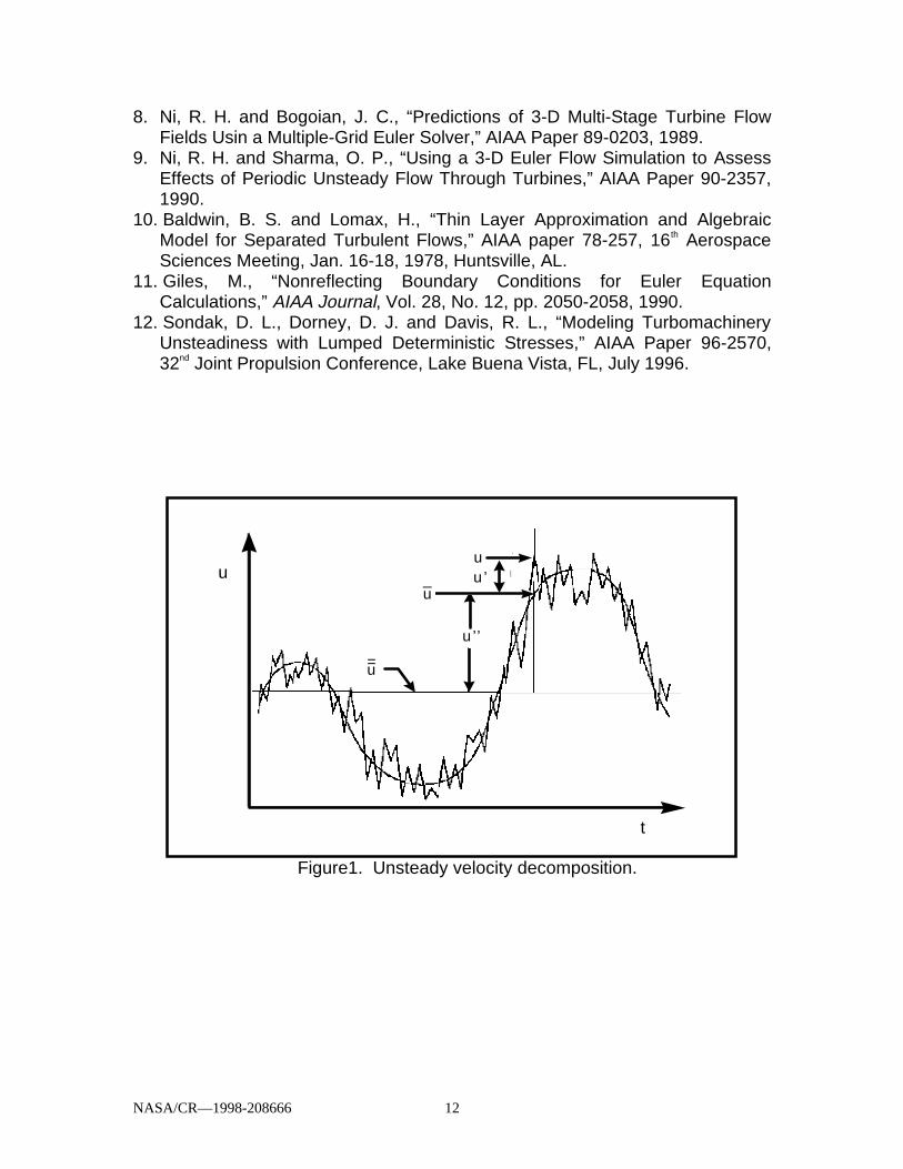
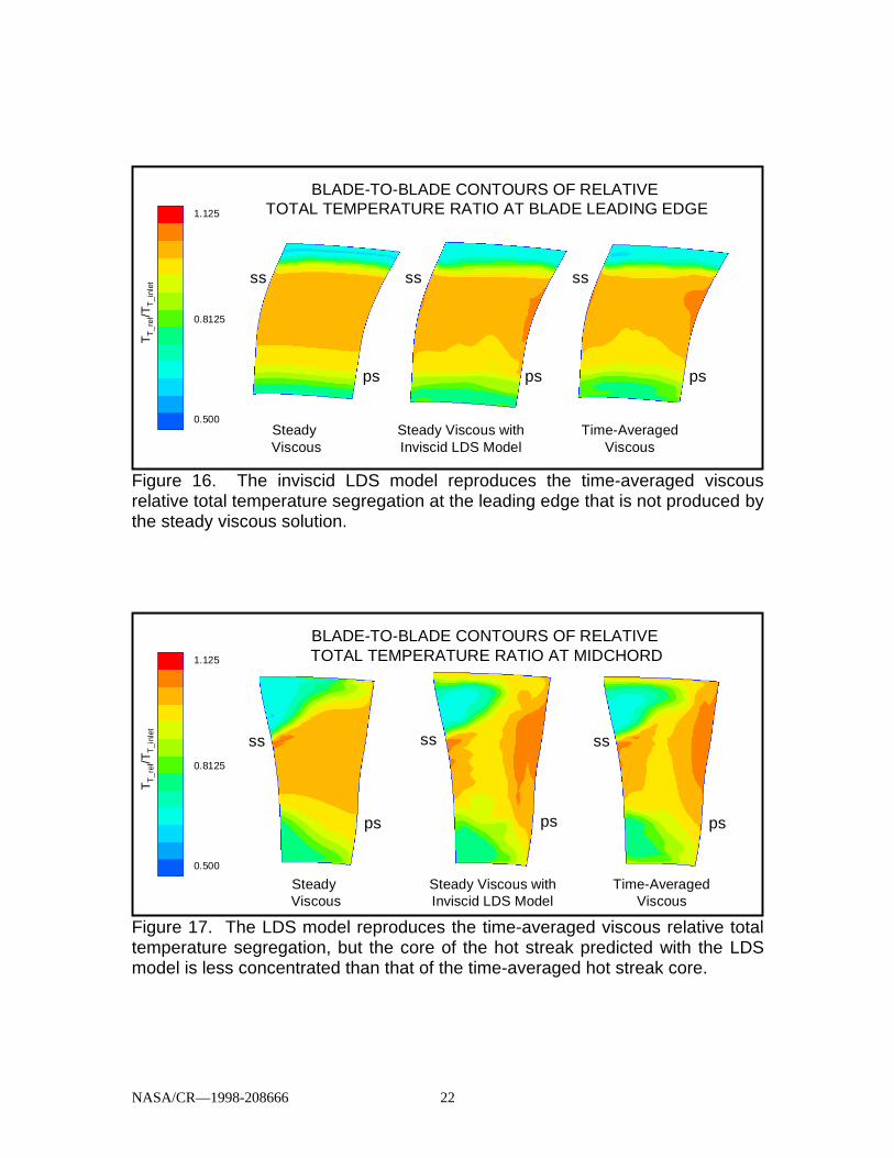
The relative total temperature distributions on the blade for the inviscid LDSmodel as well as the time-averaged and steady viscous solutions at threespanwise locations are shown in Fig. 14. The inviscid LDS model producessurface temperatures very close to the time-averaged viscous values. Near theendwalls, the inviscid LDS model predicts the same heat loads as the time-averaged viscous solution, but near midspan, the heat load predicted with theinviscid LDS model is less than that of the time-averaged viscous solution.Relative total temperature contours for the rotor pressure and suction surfacesare shown in Fig. 15. The contours indicate that the hot streak predicted withthe inviscid LDS model has less spreading of the core region on the pressuresurface than that of the time-averaged viscous solution, but matches the time-averaged viscous solution extremely well on the suction side of the blade. Blade-to-blade cuts of the relative total temperature contours at the leading edge of theblade (see Fig. 16) indicate that the inviscid LDS model reproduces the time-averaged viscous temperature segregation near the leading edge that is notproduced by the steady viscous solution. In Fig. 17, blade-to-blade cuts nearmidchord show that the core of the hot streak predicted with the LDS model issimilar to that predicted with the time-averaged viscous flow, while the steadycomputation does not produce a core flow at all. However, the core of the hotstreak predicted with the LDS model breaks apart near its lower edge with someof the core migrating to the pressure surface and some remaining just off of thepressure surface, resulting in a smaller section of the pressure side of the bladeheating up (see Fig. 15, also). The time-averaged viscous solution indicates thatthe core remains concentrated and all of it migrates to the pressure side of theblade, resulting in a larger area of the pressure side of the blade heating up.Near the trailing edge, (see Fig. 18), the behavior of the core hot streak is similarto that at midchord: The core produced with the LDS model is less concentratedthan that of the time-averaged viscous computation, resulting in a smaller areaof the blade surface heating up.

The ultimate goal of this work is to predict the effect of the hot streak on thetime-averaged temperature distribution on the outer air seal with a steadycomputation. The circumferentially averaged relative total temperatures on theouter air seal for the steady and time-averaged viscous solutions as well as thesteady viscous with the inviscid LDS model are shown in Fig. 19. The steadyviscous computation predicts cooler temperatures in the leading edge regionthan the time-averaged viscous computation. The inviscid LDS model does a

NASA/CR—1998-208666 10

good job of predicting the time-averaged viscous temperature level as well asthe location where the outer air seal begins to heat up.

As with the two-dimensional results, the steady viscous solution with the LDSmodel is significantly less expensive to compute than the unsteady viscoussolution. The computational costs for the inviscid, viscous and LDS solutions areshown in Table 2. The CPU times for the steady computations are based on6000 iterations, while those for the unsteady computations are based on 10cycles. For the unsteady inviscid and viscous solutions, 200 iterations per globalcycle and 10 (for inviscid) and 30 (viscous) inner iterations are used. The CPUrequirements for the steady viscous computations with inviscid LDS model areonly 25% of those for the unsteady viscous computations. This number is higherthan that for the two-dimensional case (3.6%), because a finer inviscid grid isrequired to resolve the three-dimensional effects.

The results presented in this section indicate that the inviscid LDS model is aviable option for predicting the time-averaged flow characteristics of a hot streakmigrating through a turbine stage and the temperature increase on the outer airseal caused by the hot streak. The inviscid LDS model does not exactlyreproduce the segregation and spreading of the hot streak core that is predictedby the time-averaged viscous flow. This deficiency may be due to the lack ofviscous effects in the inviscid LDS model. Further work is required toincorporate viscous effects into the inviscid LDS model and to examine in detailthe LDS field associated with the viscous regions. This could be achieved bycomparing the LDS field from a viscous solution with that from an inviscidsolution. Performing a parametric study of the application of the LDS models forvarious hot streak profiles may also indicate the driving mechanism behind thedifferences in the LDS solution and the time-averaged solution.

The success of the LDS model comes at the relatively low cost of theinviscid solutions. Another approach that may be even less costly is to developa new inter-blade-row boundary condition that includes the unsteady effects as asource term, similar to the implementation of the LDS model. An analyticaldescription of the source term may also be derived from the lumpeddeterministic stress terms.

Table 2. Three-dimensional CPU requirements.Total Grid Points

STEADY(CPU sec.)

UNSTEADY(CPU sec.)

TOTAL(CPU sec.)

Inviscid Grid 143,418 68,668 169,546 238,514Viscous Grid 430,122 205,942 1,525,449 1,731,391Viscous+Inviscid LDS 430,122 444,456* N/A 444,456

*CPU=Steady Inviscid+Unsteady Inviscid + Steady Viscous

NASA/CR—1998-208666 11

ConclusionsThis report has presented the results of a study into the feasibility of using

lumped deterministic stresses to model the time-averaged unsteady effects ofthe migration of a hot streak through a first stage rotor and the resulting heatload on the outer air seal. Time-averaged unsteady inviscid solutions are usedto compute the LDS model. This model is then used with a steady viscoussolution to simulate the time-averaged viscous solution. Both two-dimensionaland three-dimensional models are examined. The two-dimensional resultsindicate that the inviscid LDS model can simulate the time-averaged viscoussolutions at a significant reduction in CPU costs. The three-dimensional resultsshow that the inviscid LDS model does a good job of predicting the migrationand segregation of the hot streak as well as the increased heat load on the outerair seal. These three-dimensional results can also be obtained at a significantsavings in CPU.

The effect of the tip leakage flow was not included in these computationsand should be addressed. Other areas that need to be examined includeincorporating viscous effects into the LDS model and developing a new inter-blade-row boundary condition that includes the LDS model for the unsteadyeffects. Performing a parametric study of the application of the LDS models forvarious hot streaks would also provide insight into the development of ananalytical model. This work was scheduled to be performed in phase IV of thisprogram but has been discontinued due to a lack of funding.

References1. Saxer, A. P. and Felici, H. M., “Numerical Analysis of 3-D Unsteady Hot

Streak Migration and Shock Interaction in a Turbine Stage,” ASME Paper94-GT-76, International Gas Turbine and Aeroengine Congress andExposition, The Hague, Netherlands, June 1994.

2. Dorney, D. J., Davis, R. L. and Edwards, D. E., “Unsteady Analysis of HotStreak Migration in a Turbine Stage,” Journal of Propulsion and Power, Vol.8, No. 2, March-April 1992, pp. 520-529.

3. Rai, M. M. and Dring, R. P., “Navier-Stokes Analyses of the Redistribution ofInlet Temperature Distortions in a Turbine,” Journal of Propulsion and Power,Vol. 6, May-June 1990.

4. Takahashi, R. and Ni, R. H., “Unsteady Hot Streak Simulation Through 1-1/2Stage Turbine,” AIAA Paper 91-3382, 1991.

5. Adamczyk, J. J., “Model Equation for Simulating Flows in MultistageTurbomachinery,” ASME paper 85-GT-226, Gas Turbine Conference andExhibit, Houston, TX, March 18-21, 1985.

6. Davis, R. L., Shang, T., Buteau, J. and Ni, R. H., “Prediction of 3-D UnsteadyFlow in Multi-Stage Turbomachinery Using an Implicit Dual Time-StepApproach,” AIAA Paper 96-2565, 1996.

7. Ni, R. H., “A Multiple Grid Scheme for Solving the Euler Equations,” AIAAJournal, Vol. 20, No. 11, pp. 1565-1571, 1981.

NASA/CR—1998-208666 12

8. Ni, R. H. and Bogoian, J. C., “Predictions of 3-D Multi-Stage Turbine FlowFields Usin a Multiple-Grid Euler Solver,” AIAA Paper 89-0203, 1989.

9. Ni, R. H. and Sharma, O. P., “Using a 3-D Euler Flow Simulation to AssessEffects of Periodic Unsteady Flow Through Turbines,” AIAA Paper 90-2357,1990.

10. Baldwin, B. S. and Lomax, H., “Thin Layer Approximation and AlgebraicModel for Separated Turbulent Flows,” AIAA paper 78-257, 16th AerospaceSciences Meeting, Jan. 16-18, 1978, Huntsville, AL.

11. Giles, M., “Nonreflecting Boundary Conditions for Euler EquationCalculations,” AIAA Journal, Vol. 28, No. 12, pp. 2050-2058, 1990.

12. Sondak, D. L., Dorney, D. J. and Davis, R. L., “Modeling TurbomachineryUnsteadiness with Lumped Deterministic Stresses,” AIAA Paper 96-2570,32nd Joint Propulsion Conference, Lake Buena Vista, FL, July 1996.

u ’’

u=

u_ u ’

uu

t

u ’

Figure1. Unsteady velocity decomposition.

NASA/CR—1998-208666 13

Eu le r G rid1st Vane 49x17x3B lade 49x17x32nd V ane 49x17x3

N avie r-S tokes G rid1st Vane 121x65x3B lade 121x65x32nd V ane 129x65x3

Figure 2. Two dimensional inviscid and viscous grid distributions for a 1 ½ stageturbine.

3.0 3.5 4.0 4.5 5.0Axial Location

725

730

735

740

745

750

Rel

ativ

e To

tal T

empe

ratu

re [R

anki

ne]

Time−Averaged EulerSteady EulerSteady Euler with LDS Model

Figure 3. Two-dimensional LDS terms applied to inviscid steady simulationexactly reproduce the time-averaged relative total temperature distribution on theblade surface.

NASA/CR—1998-208666 14

EULER

NAVIER-STOKES

COMPUTATIONALMESH

ENERGY LUMPEDDETERMINISTIC STRESS

INTERPOLATEDONTO

Figure 4. Two-dimensional inviscid LDS field (energy field shown) areinterpolated from the inviscid to viscous mesh.

All LDS Terms Continuity LDSTerms

Axial MomentumLDS Terms

Tangential MomentumLDS Terms

EnergyLDS terms

Figure 5. The hot streak migration and segregation are dominated by the energyLDS terms.

NASA/CR—1998-208666 15

t im e a v e ra g e

L D S

s te a d y

1 .0 8

1 .0 4

1 .0 0

0 .9 62 .8 3 .6 4 .4 5 .2

X

T/T

t_re

lU n s te a d y V is c o u s(T im e -A v e r a g e d )

S te a d y V is c o u s w ithIn v is c id L D S

S te a d y V is c o u s

Figure 6. Inviscid LDS field applied to steady two-dimensional viscoussimulation reproduces the time-averaged relative total temperature distributionon the rotor blade.

STEADY TIME-AVERAGE STEADY with LUMPEDDETERMINISTIC STRESSES

680 780deg. R

Steady Viscous Unsteady Viscous(Time-Averaged)

Steady Viscous withInviscid LDS

0.92 1.05

T/Tt_rel

Figure 7. Inviscid LDS terms applied to a steady two-dimensional viscoussimulation reproduce the time-averaged segregation of the relative totaltemperature in the rotor blade.

NASA/CR—1998-208666 16

k-plane

i-plane

Inviscid GridVane 49x33x41Blade 57x33x41

Viscous GridVane 81x49x57Blade 73x49x57

Figure 8. Inviscid and viscous grid distributions for three-dimensionalapplication.

0 1000 2000 3000Iterations

10−6

10−5

10−4

10−3

10−2

10−1

Con

verg

ence

Figure 9. The convergence history for steady inviscid solution with inviscid LDSmodel indicates that the addition of the LDS source terms does not causeinstabilities in the solution.

NASA/CR—1998-208666 17

0.8 1.0 1.2 1.4 1.6 1.8Axial Distance

0.50

0.60

0.70

0.80

0.90

1.00

1.10

TO

rel/T

Oin

let

Time−Averaged InviscidSteady InviscidSteady Inviscid with Inviscid LDS

Pressure Surface of Blade

Suction Surface of Blade

10a.) 20% span

0.8 1.0 1.2 1.4 1.6 1.8Axial Distance

0.95

0.97

1.00

1.02

1.05

1.07

1.10

T Ore

l/TO

inle

t

Time−Averaged InviscidSteady InviscidSteady Inviscid with Inviscid LDS

Pressure Surface of Blade

Suction Surface of Blade

10b.) 50% span

NASA/CR—1998-208666 18

0.8 1.0 1.2 1.4 1.6 1.8Axial Distance

0.50

0.60

0.70

0.80

0.90

1.00

1.10

T Ore

l/TO

inle

t

Time−Averaged InviscidSteady InviscidSteady Inviscid with Inviscid LDS

Pressure Surface of Blade

Suction Surfaceof Blade

10c.) 80% spanFigure 10. Three-dimensional inviscid LDS model applied to an inviscid steadysimulation EXACTLY reproduces the time-averaged relative total temperaturedistribution on the rotor blade.

Steady Inviscid Time-AverageInviscid

Steady Invsicid with Inviscid LDS Model

Figure 11. Three-dimensional inviscid LDS field applied to an inviscid steadysimulation EXACTLY reproduces the time-averaged relative total temperaturesegregation in the passage at midspan.

NASA/CR—1998-208666 19

Interpolated Interpolated

Inviscid InviscidViscous Viscous

Figure 12. Three-dimensional energy deterministic stress field from inviscid gridinterpolated onto viscous grid.

0 1000 2000 3000 4000 5000 6000Iterations

10−5

10−4

10−3

10−2

10−1

100

Conv

erge

nce

Steady Viscous with Inviscid LDSSteady Viscous

Figure 13. The convergence history for the steady three-dimensional viscoussolution with inviscid LDS model shows that the additional source term does notcause instabilities in the solution.

NASA/CR—1998-208666 20

0.8 1.0 1.2 1.4 1.6 1.8Axial Distance

0.50

0.60

0.70

0.80

0.90

1.00

1.10

T Ore

l/TO

inle

t

Time−Averaged ViscousSteady ViscousSteady Viscous with Inviscid LDS

PS

SS

14a.) 20% span

0.8 1.0 1.2 1.4 1.6 1.8Axial Distance

0.90

0.95

1.00

1.05

1.10

T Ore

l/TO

inle

t

Time−Averaged ViscousSteady ViscousSteady Viscous with Inviscid LDS

PS

SS

PS

PSSS

14b.) 50% span

NASA/CR—1998-208666 21

0.8 1.0 1.2 1.4 1.6 1.8Axial Distance

0.40

0.50

0.60

0.70

0.80

0.90

1.00

1.10

T Ore

l/TO

inle

t

Time−Averaged ViscousSteady ViscousSteady Viscous with Inviscid LDS

PS

SS

14c.) 80% spanFigure 14. Three-dimensional steady viscous solution with inviscid LDS modeldoes a good job of reproducing the time-averaged relative total temperaturedistribution on the blade.

Pressure Side

Tim e-Averaged Viscous

Suction Side

Steady Viscous

Steady Viscous with Inviscid LDS M odel

T im e-Averaged Viscous

SteadyViscous

Steady Viscous with Inviscid LDS M odel

1.125

0.500

0.8125

TT

_re

l/TT

_in

let

Figure 15. The relative total temperature contours on the rotor surface indicatethat the inviscid LDS model predicts the time-averaged accumulation of the hotstreak on the pressure side, but under-predicts the spreading of the hot streak.

NASA/CR—1998-208666 22

1.125

0.500

0.8125

TT

_rel/T

T_i

nlet

Steady Viscous

Steady Viscous withInviscid LDS Model

BLADE-TO-BLADE CONTOURS OF RELATIVE TOTAL TEMPERATURE RATIO AT BLADE LEADING EDGE

ss

ps

ss

Time-AveragedViscous

ps ps

ssss

Figure 16. The inviscid LDS model reproduces the time-averaged viscousrelative total temperature segregation at the leading edge that is not produced bythe steady viscous solution.

1.125

0.500

0.8125

TT

_rel/T

T_i

nlet

Steady Viscous

Steady Viscous withInviscid LDS Model

BLADE-TO-BLADE CONTOURS OF RELATIVE TOTAL TEMPERATURE RATIO AT MIDCHORD

ss

ps

ss

Time-AveragedViscous

ps ps

ssss

Figure 17. The LDS model reproduces the time-averaged viscous relative totaltemperature segregation, but the core of the hot streak predicted with the LDSmodel is less concentrated than that of the time-averaged hot streak core.

NASA/CR—1998-208666 23

1.125

0.500

0.8125

TT

_rel/T

T_i

nlet

Steady Viscous

Steady Viscous withInviscid LDS Model

BLADE-TO-BLADE CONTOURS OF RELATIVE TOTAL TEMPERATURE RATIO AT BLADE TRAILING EDGE

ss

ps

ss

Time-AveragedViscous

ps ps

ssss

Figure 18. The inviscid LDS model indicates that that the hot streak completelysegregates by the time it reaches the trailing edge, while the time-averagedviscous flow shows some hot flow in the core region.

0.5 1.0 1.5 2.0 2.5Axial Distance

0.5

0.6

0.7

0.8

0.9

1.0

1.1

Circ

umfe

rent

ially

Ave

rage

d T O

rel/T

Oin

let

Time−Averaged ViscousSteady ViscousSteady Viscous with inviscid LDS

LeadingEdge

TrailingEdge

Figure 19. The inviscid LDS model shows the same relative total temperaturelevels and location of increased heating on the outer air seal as the time-averaged viscous relative total temperature distribution, while the steady viscoussolution under-predicts the temperature at all axial locations and delays the heatbuildup until almost mid-chord.

This publication is available from the NASA Center for AeroSpace Information, (301) 621–0390.

REPORT DOCUMENTATION PAGE

2. REPORT DATE

19. SECURITY CLASSIFICATION OF ABSTRACT

18. SECURITY CLASSIFICATION OF THIS PAGE

Public reporting burden for this collection of information is estimated to average 1 hour per response, including the time for reviewing instructions, searching existing data sources,gathering and maintaining the data needed, and completing and reviewing the collection of information. Send comments regarding this burden estimate or any other aspect of thiscollection of information, including suggestions for reducing this burden, to Washington Headquarters Services, Directorate for Information Operations and Reports, 1215 JeffersonDavis Highway, Suite 1204, Arlington, VA 22202-4302, and to the Office of Management and Budget, Paperwork Reduction Project (0704-0188), Washington, DC 20503.

NSN 7540-01-280-5500 Standard Form 298 (Rev. 2-89)Prescribed by ANSI Std. Z39-18298-102

Form Approved

OMB No. 0704-0188

12b. DISTRIBUTION CODE

8. PERFORMING ORGANIZATION REPORT NUMBER

5. FUNDING NUMBERS

3. REPORT TYPE AND DATES COVERED

4. TITLE AND SUBTITLE

6. AUTHOR(S)

7. PERFORMING ORGANIZATION NAME(S) AND ADDRESS(ES)

11. SUPPLEMENTARY NOTES

12a. DISTRIBUTION/AVAILABILITY STATEMENT

13. ABSTRACT (Maximum 200 words)

14. SUBJECT TERMS

17. SECURITY CLASSIFICATION OF REPORT

16. PRICE CODE

15. NUMBER OF PAGES

20. LIMITATION OF ABSTRACT

Unclassified Unclassified

Final Contractor Report

Unclassified

1. AGENCY USE ONLY (Leave blank)

10. SPONSORING/MONITORING AGENCY REPORT NUMBER

9. SPONSORING/MONITORING AGENCY NAME(S) AND ADDRESS(ES)

National Aeronautics and Space AdministrationLewis Research CenterCleveland, Ohio 44135–3191

October 1998

NASA CR—1998-208666UTRC Report 98–07

E–11377

29

A03

Deterministic Stress Modeling of Hot Gas Segregation in a Turbine

Judy Busby, Doug Sondak, Brent Staubach, and Roger Davis

Turbine; Computational fluid dynamics; CFD; Simulation

WU–509–10–11–00NAS3–26618 Task Order 28

United Technologies Research Center, Pratt & Whitney411 Silver LaneEast Hartford, Connecticut 06108

Unclassified -UnlimitedSubject Categories: 77 and 66 Distribution: Nonstandard

Simulation of unsteady viscous turbomachinery flowfields is presently impractical as a design tool due to the long runtimes required. Designers rely predominantly on steady-state simulations, but these simulations do not account for someof the important unsteady flow physics. Unsteady flow effects can be modeled as source terms in the steady flowequations. These source terms, referred to as Lumped Deterministic Stresses (LDS), can be used to drive steady flowsolution procedures to reproduce the time-average of an unsteady flow solution. The goal of this work is to investigatethe feasibility of using inviscid lumped deterministic stresses to model unsteady combustion hot streak migration effectson the turbine blade tip and outer air seal heat loads using a steady computational approach. The LDS model is obtainedfrom an unsteady inviscid calculation. The LDS model is then used with a steady viscous computation to simulate thetime-averaged viscous solution. Both two-dimensional and three-dimensional applications are examined. The inviscidLDS model produces good results for the two-dimensional case and requires less than 10% of the CPU time of theunsteady viscous run. For the three-dimensional case, the LDS model does a good job of reproducing the time-averagedviscous temperature migration and separation as well as heat load on the outer air seal at a CPU cost that is 25% of thatof an unsteady viscous computation.

Project Manager, Joseph P. Veres, Computing and Interdisciplinary Systems Office, NASA Lewis Research Center,organization code 2900, (216) 433–2436.