DETERMINISTIC POLYNOMIAL IDENTITY TESTS FOR …
82
DETERMINISTIC POLYNOMIAL IDENTITY TESTS FOR MULTILINEAR BOUNDED-READ FORMULAE Matthew Anderson, Dieter van Melkebeek, and Ilya Volkovich June 20, 2014 Abstract. We present a polynomial-time deterministic algorithm for testing whether constant-read multilinear arithmetic formulae are iden- tically zero. In such a formula each variable occurs only a constant num- ber of times and each subformula computes a multilinear polynomial. Our algorithm runs in time s O(1) · n k O(k) , where s denotes the size of the formula, n denotes the number of variables, and k bounds the number of occurrences of each variable. Before our work no subexponential-time deterministic algorithm was known for this class of formulae. We also present a deterministic algorithm that works in a blackbox fashion and runs in time n k O(k) +O(k log n) in general, and time n k O(k 2 ) +O(kD) for depth D. Finally, we extend our results and allow the inputs to be replaced with sparse polynomials. Our results encompass recent deterministic identity tests for sums of a constant number of read-once formulae, and for multilinear depth-four formulae. Keywords. Derandomization, Identity Testing, Arithmetic Circuits, Bounded-Depth Circuits Subject classification. 12Y05, 68Q25
Transcript of DETERMINISTIC POLYNOMIAL IDENTITY TESTS FOR …
DETERMINISTIC POLYNOMIAL
IDENTITY TESTS FOR
MULTILINEAR BOUNDED-READ
FORMULAE
Matthew Anderson, Dieter van Melkebeek,
and Ilya Volkovich
June 20, 2014
Abstract. We present a polynomial-time deterministic algorithm fortesting whether constant-read multilinear arithmetic formulae are iden-tically zero. In such a formula each variable occurs only a constant num-ber of times and each subformula computes a multilinear polynomial.Our algorithm runs in time sO(1) ·nkO(k)
, where s denotes the size of theformula, n denotes the number of variables, and k bounds the numberof occurrences of each variable. Before our work no subexponential-timedeterministic algorithm was known for this class of formulae. We alsopresent a deterministic algorithm that works in a blackbox fashion and
runs in time nkO(k)+O(k logn) in general, and time nk
O(k2)+O(kD) for depthD. Finally, we extend our results and allow the inputs to be replacedwith sparse polynomials. Our results encompass recent deterministicidentity tests for sums of a constant number of read-once formulae, andfor multilinear depth-four formulae.
Keywords. Derandomization, Identity Testing, Arithmetic Circuits,Bounded-Depth Circuits
Subject classification. 12Y05, 68Q25

2 Anderson, van Melkebeek & Volkovich
1. Introduction
Polynomial identity testing (PIT) denotes the fundamental prob-lem of deciding whether a given polynomial identity holds. Moreprecisely, we are given an arithmetic circuit or formula F on ninputs over a given field F, and we wish to know whether all thecoefficients of the formal polynomial P , computed by F , vanish.Due to its basic nature, PIT shows up in many constructions inthe theory of computing. Particular problems that reduce to PITinclude integer primality testing (Agrawal & Biswas 2003) and find-ing perfect matchings in graphs (Lovasz 1979).
PIT has a very natural randomized algorithm – pick valuesfor the variables uniformly at random from a small set S, andaccept iff P evaluates to zero on that input. If P ≡ 0 then thealgorithm never errs; if P 6≡ 0 then by Schwartz-Zippel (DeMillo& Lipton 1978; Schwartz 1980; Zippel 1979) the probability of anerror is at most d/|S|, where d denotes the total degree of P . Thisresults in an efficient randomized algorithm for PIT. The algorithmworks in a blackbox fashion in the sense that it does not access therepresentation of the polynomial P , rather it only examines thevalue of P at certain points (from F or an extension field of F).
Despite the simplicity of the above randomized algorithm andmuch work over the course of thirty years, no efficient deterministicalgorithm is known when the polynomial is given as an arithmeticformula.
Is there an efficient deterministic identity test forarithmetic formulae?
The question is central to the pursuit of circuit lower bounds.Efficiently derandomizing identity testing implies Boolean or arith-metic formula/circuit lower bounds that have been elusive for halfa century (Aaronson & van Melkebeek 2011; Kabanets & Impagli-azzo 2004; Kinne et al. 2012). In fact, an efficient deterministicblackbox identity test for arithmetic formulae of depth three orfour already implies such lower bounds (Agrawal & Vinay 2008;Gupta et al. 2013). Conversely, the well-known hardness vs ran-domness tradeoffs imply that sufficiently strong Boolean circuit

PIT for Multilinear Bounded-Read Formulae 3
lower bounds yield efficient deterministic polynomial identity tests,and there are a couple of similar results starting from arithmeticcircuit lower bounds as well (Dvir et al. 2009; Kabanets & Impagli-azzo 2004).
The powerful connections with circuit lower bounds have en-ergized much of the recent effort towards derandomizing iden-tity testing for restricted classes of arithmetic formulae, in par-ticular for constant-depth formulae. For depth-two formulae sev-eral deterministic polynomial-time blackbox algorithms are known(Agrawal 2003; Arvind & Mukhopadhyay 2010; Ben-Or & Tiwari1988; Blaser et al. 2009; Klivans & Spielman 2001). For depth threethe state of the art is a deterministic polynomial-time blackbox al-gorithm when the fanin of the top gate is fixed to any constant(Saxena & Seshadhri 2012). The same is known for depth fourwhen the formulae are multilinear, i.e., when every gate in the for-mula computes a polynomial of degree at most one in each variable(Saraf & Volkovich 2011). There are also a few incomparable re-sults for rather specialized classes of depth-four formulae (Arvind& Mukhopadhyay 2010; Saxena 2008; Shpilka & Volkovich 2009).We refer to the excellent survey papers (Saxena 2009; Shpilka &Yehudayoff 2010) for more information.
Another natural restriction is to bound the number of timeseach variable can occur in the formula. We call such a restrictedformula read-k, where k denotes the maximum number of timeseach variable may appear. Identity testing for read-once formulaeis trivial in the non-blackbox setting as there can be no cancel-lation of monomials. Shpilka and Volkovich considered a specialtype of bounded-read formulae, namely formulae that are the sumof k read-once formulae. For such formulae and constant k theyestablished a deterministic polynomial-time non-blackbox identitytest as well as a deterministic blackbox algorithm that runs inquasi-polynomial time, more precisely in time sO(log s), on formu-lae of size s (Shpilka & Volkovich 2008, 2009). These results havebeen extended to sums of k read-once algebraic branching pro-grams (Jansen et al. 2009). Algebraic branching programs are amodel of computation analogous to Boolean branching programsand lying between formulae and circuits in terms of power.

4 Anderson, van Melkebeek & Volkovich
1.1. Results. We present a deterministic polynomial-time iden-tity test for multilinear constant-read formulae, as well as a deter-ministic quasi-polynomial-time blackbox algorithm for these for-mulae.
Theorem 1.1 (Main Result). For each constant k ∈ N thereis a deterministic polynomial identity test for multilinear read-kformulae of size s that runs in time poly(s). In addition, there isa deterministic blackbox test that runs in time sO(log s).
Note that Theorem 1.1 extends the class of formulae that Shpilkaand Volkovich could handle since a sum of read-once formulae isalways multilinear. This is a strict extension; in Section 2.1.3 weexhibit an explicit multilinear read-twice formula with n variablesthat requires Ω(n) terms when written as a sum of read-once for-mulae. The separating example also shows that the efficiency of theidentity test in Theorem 1.1 cannot be obtained by first expressingthe given formula as a sum of read-once formulae and then apply-ing the known algorithms for sums of read-once formulae (Shpilka& Volkovich 2009) to it.
Shpilka and Volkovich actually proved their result for sums ofa somewhat more general type than read-once formulae, namelyread-once formulae in which each leaf variable is replaced by alow-degree univariate polynomial in that variable. We can handle afurther extension in which the leaf variables are replaced by sparsemultivariate polynomials. We use the term sparse-substituted for-mula for a formula along with substitutions for the leaf variablesby multivariate polynomials, where we assume that the substitutedpolynomials are each given as a list of terms (monomials). We calla sparse-substituted formula read-k if each variable appears in atmost k of those multivariate polynomials. The substituted polyno-mials need not be multilinear, as long as for every multiplicationgate of the original formula the different input branches of thegate are variable disjoint. We call such sparse-substituted formu-lae structurally-multilinear.
Theorem 1.2 (Extended Main Result). For each constant k ∈N there is a deterministic polynomial identity test for structurally-multilinear sparse-substituted read-k formulae that runs in time

PIT for Multilinear Bounded-Read Formulae 5
sO(log t), where s denotes the size of the formula, and t the maximumnumber of terms a substitution consists of. In addition, there is adeterministic blackbox test that runs in time sO(log st).
We observe that any multilinear depth-four alternating formulawith an addition gate of fanin k as the output can be writtenas the sum of k sparse-substituted read-once formulae, where theread-once formulae are single monomials and the substitutions cor-respond to multilinear depth-two formulae. This implies that ourblackbox algorithm also extends the work by Karnin et al. (2013),who established a deterministic quasi-polynomial-time blackbox al-gorithm for multilinear formulae of depth four. Thus, our resultscan be seen as unifying identity tests for sums of read-once formu-lae (Shpilka & Volkovich 2009) with identity tests for depth-fourmultilinear formulae (Karnin et al. 2013) while achieving compa-rable running times in each of those restricted settings. It remainsan open question whether our results can be extended to test mul-tilinear read-k algebraic branching programs in a way analogousto the extension from Shpilka & Volkovich (2009) to Jansen et al.(2009).
We can improve the running time of our blackbox algorithmin the case where the formulae have small depth. In particular,we obtain a polynomial-time blackbox algorithm for multilinearconstant-read constant-depth formulae and, for the special case offields with infinite characteristic, Agrawal et al. (2012) recentlyshowed that the multilinearity condition can be removed. We referto Section 6.3 for more details about those results, and to the restof Section 6 for more general versions and finer parameterizationsof our main result and its extensions.
1.2. Techniques. We now give an overview of our approachwith a focus on the deterministic polynomial identity tests for mul-tilinear read-k formulae given in Theorem 1.1. Both the blackboxand the non-blackbox algorithms are obtained by induction on k,using known algorithms in the base case of read-once formulae. Tolift the identity tests for read-once formulae we exhibit reductionsfrom testing multilinear read-(k+1) formulae to testing multilinearread-k formulae. Applying the transformation k times thus reduces

6 Anderson, van Melkebeek & Volkovich
identity testing multilinear read-(k+1) formulae to identity testingread-once formulae. At each stage the transformation consists ofthe following two steps, where the intermediate instances are sumsof two multilinear read-k formulae, which we refer to as multilinearΣ2-read-k formulae.
Step 1: Reduce multilinear read-(k+1) formulae PIT to multilinearΣ2-read-k formulae PIT.
Step 2: Reduce multilinear Σ2-read-k formulae PIT to multilinearread-k formulae PIT.
We first explain the blackbox reductions, then discuss the moreefficient but non-blackbox variant, and finally sketch the extensiongiven by Theorem 1.2.
1.2.1. Blackbox setting. A deterministic blackbox polynomialidentity test for a class F of formulae is known to be equivalent toa so-called hitting set generator for F (see, e.g., Shpilka & Yehu-dayoff (2010, Lemma 4.1)). The latter is a uniform collection ofpolynomial maps Gn : F`(n) → Fn, one for every positive integern, such that Gn hits all formulae from F on n variables, i.e., forevery non-zero formula F in F on n variables, F (Gn) is a non-zeropolynomial. We only need one direction of the equivalence, whichfollows from the Schwartz-Zippel lemma: Given a hitting set gen-erator Gn of total degree dGn for F , we can deterministically testwhether a formula F in F of total degree dF on n variables is iden-tically zero by picking an arbitrary subset S of size dF · dGn + 1from F (or an extension field of F) and checking that F (Gn(x)) = 0for every x ∈ S`(n). For a multilinear formula F , the total degreedF is at most n, and the running time of the resulting blackboxidentity test is nO(`(n)) as long as the generator is computable inthat amount of time, and has total degree dGn that is polynomiallybounded.
Base case and generalization. For read-once formulae, Shpilka &Volkovich (2009) defined a polynomial-time computable polyno-mial map Gn,w : F2w → Fn of total degree n over a field F, andshowed that Gn,dlogne+1 hits read-once formulae on n variables. Werefer to Gn,w as the SV-generator. By the above connection, the
PIT for Multilinear Bounded-Read Formulae 7
SV-generator yields a deterministic blackbox identity test for read-once formulae that runs in time nO(logn).
Using various additional properties of the SV-generator, weargue by induction on k that, for some function f : N → N,Gn,f(k)+kdlogne hits multilinear read-k formulae on n variables. Bythe same token, this yields a blackbox identity test for multilinearread-k formulae that runs in time nO(logn) for every fixed k. Wenow explain the two inductive steps in this setting.
Step 1. We show that if Gn,w hits multilinear Σ2-read-k formu-lae on n variables, then Gn,w+dlogne hits multilinear read-(k + 1)formulae on n variables. In order to do so, we exploit the prop-erty of the SV-generator that if Gn,w hits a non-zero first-orderpartial derivative of a formula, then Gn,w+1 hits the formula itself.We show that for every non-constant multilinear read-(k + 1) for-mula F , there exists a variable x such that the partial derivative∂xF of F with respect to x is non-zero and can be written as theproduct of (i) subformulae of F each depending on at most halfof the variables, and (ii) a multilinear Σ2-read-k formula which isthe partial derivative of a subformula of F . We call this process ofbreaking up a formula via a well-chosen partial derivative fragmen-tation (this generalizes a technique of Karnin et al. (2013)). Notethat the factors of type (i) are multilinear read-(k + 1) formulaethemselves. By recursively fragmenting those factors dlog ne times,they become constant and are hit by Gn,w for trivial reasons. Thefactors of type (ii) are hit by Gn,w by assumption. Since a hit-ting set generator for a class of formulae also hits all products offormulae from that class (because polynomial rings over fields areintegral domains), inductively applying the above property of theSV-generator shows that Gn,w+dlogne hits the original multilinearread-(k + 1) formula F .
Step 2. We show that, for some function h : N → N, if Gn,w hitsmultilinear read-k formulae on n variables, then Gn,w+h(k) hits mul-tilinear Σ2-read-k formulae on n variables. In order to do so, we ex-ploit another property of the SV-generator. By a zero-substitutionof a polynomial Q we mean the polynomial obtained from Q bysetting some (possibly all or none) of the variables to zero. TheSV-generator Gn,w′ has the property that it hits every non-zero

8 Anderson, van Melkebeek & Volkovich
polynomial Q on n variables that satisfies the following condition:no zero-substitution of Q equals a monomial of more than w′ vari-ables. The intuition for applying this property is that, no matterwhat the non-zero formula F looks like, for a random assignmentσ the shifted formula F (x+σ) satisfies the condition, and is there-fore hit by Gn,w′ . Moreover, the following key lemma shows thatin the case of a multilinear Σ2-read-k formula F , the only way thecondition can fail is if σ happens to be a zero of one of the non-zeropartial derivatives of small order of a nontrivial subformula of F .
Lemma 1.3 (Simplified Key Lemma). There is a function h :N → N such that for every multilinear Σ2-read-k formula F withvariables x, and variable assignment σ where none of the non-zeropartial derivatives of order h(k) of any nontrivial subformula of Fvanish, the zero-substitutions of F (x + σ) are not monomials ofmore than h(k) variables.
Observe that all nontrivial subformulae of a multilinear Σ2-read-k formula F are multilinear and read-k, as are their partialderivatives, because multilinear read-k formulae are closed underderivatives. Now, we assumed that Gn,w hits multilinear read-k for-mulae on n variables, and therefore also products of such formulae.Thus, a common non-zero of the non-zero partial derivatives of or-der h(k) of the nontrivial subformulae of F appears in the image ofGn,w. By Lemma 1.3 and the above property of the SV-generator,this means that for some σ in the image of Gn,w, the SV-generatorGn,w′ with w′ = h(k) hits the shifted formula F (x + σ). Thisimplies that F (Gn,w′ +Gn,w) 6≡ 0, where Gn,w′ +Gn,w denotes thecomponent-wise sum of the polynomial mapsGn,w′ andGn,w on dis-joint sets of variables. Yet another property of the SV-generator isits additivity: Gn,w′ + Gn,w = Gn,w′+w. We conclude that Gn,w′+w
with w′ = h(k) hits F .
By combining the two steps, we conclude that if Gn,w hits mul-tilinear read-k formulae on n variables, then Gn,w+h(k)+dlogne hitsmultilinear read-(k + 1) formulae on n variables. When we ap-ply this combination k − 1 times starting from the SV-generatorfor read-once formulae, and simplify using the additivity propertyof the SV-generator, we obtain that Gn,f(k)+kdlogne hits multilin-
PIT for Multilinear Bounded-Read Formulae 9
ear read-k formulae on n variables, where f(k) =∑k−1
i=0 h(i). Thisyields our hitting set generator for multilinear read-k formulae.
Proving the Key Lemma. Let us briefly sketch the proof ofLemma 1.3. Let F be a multilinear Σ2-read-k formula and letσ be an assignment for F of the type specified in the statementof the lemma. Ignoring zero substitutions for simplicity, supposeF (x + σ) is identical to a monomial MV
.=∏
i∈V xi. The identityF (x + σ) ≡ MV must hold with respect to partial derivatives ∂Pfor any set P ⊆ V . Moreover, (∂PF )(x + σ) ≡ ∂P (F (x + σ)) ≡∂PMV = MV \P . We argue that provided |V | is at least a suffi-ciently large function h(k), there exists a set P ⊆ V witnessingthat (∂PF )(x + σ) −MV \P is not identically zero. Similar to theapproach of Karnin et al. (2013), our witness for non-identity isa structural one: We show that ∂PF can be rewritten in such away that its structure alone indicates that (∂PF )(x + σ) is not amonomial. The selection of P and the rewriting of ∂PF are compo-nents of the most intricate technical transformation in our paper.We call it shattering as it is accomplished, in part, by repeatedlyfragmenting the summands of F . (Recall that fragmenting is ourprocess of breaking up a formula via a well-chosen partial deriva-tive.) We refer to Section 3.4 for more intuition about this keypart of our paper.
1.2.2. Non-Blackbox Setting. When we are given access tothe input formula itself, we can improve the running time forour deterministic identity test for multilinear read-k formulae fromquasi-polynomial to polynomial.
In the non-blackbox setting, the case of read-once formulae istrivial. Since every variable occurs at most once, there is no cancel-lation of monomials at addition gates, and the only way a monomialcan vanish is if it gets multiplied by a zero polynomial at a multi-plication gate. If we iterate over the subformulae in a bottom-upfashion, this allows us to determine for each subformula whetherit is zero. This yields a simple polynomial-time identity test forread-once formulae, which forms the base case for our inductiveconstruction. We now explain how the two inductive steps men-tioned above work in the non-blackbox setting.
10 Anderson, van Melkebeek & Volkovich
Step 1. This reduction follows from a generalization of the simplealgorithm for read-once formulae, based on the following intuition:Given a multilinear read-(k + 1) formula F , if an addition gatehas an input g that contains all k+ 1 occurrences of some variablex, and g depends on x, then g cannot be cancelled at this gate.This implies that g can be replaced by a fresh variable withoutchanging whether the overall polynomial is zero. For k ≥ 1 thisallows us to transform the formula in a bottom-up fashion intoone where each addition gate is a multilinear Σ2-read-k formulawithout affecting zeroness. During the process, we just need to beable to determine for each transformed addition gate whether it iszero, and if not, what variables it depends on. Both of these tasksreduce to PIT for multilinear Σ2-read-k formulae. This yields apolynomial-time reduction from PIT for multilinear read-(k + 1)formulae to PIT for multilinear Σ2-read-k formulae. This consti-tutes an improvement over the corresponding blackbox reductionwhich adds a logarithmic term to the seed length of the generator,and therefore a quasi-polynomial factor to the running time of theidentity test.
Step 2. The blackbox version of this step is already efficient as eachapplication adds only a constant amount to the seed length of thegenerator and therefore only a polynomial factor to the runningtime of the identity test. Thus, it suffices to simulate the behav-ior of the blackbox reduction on a multilinear Σ2-read-k formulaF with n variables. To this end we explicitly compute a com-mon non-zero σ of the at most nh(k) non-zero partial derivativesof the subformulae of F up to order h(k), using the assumed non-blackbox identity test for multilinear read-k formulae combinedwith the standard search-to-decision reduction for PIT. We con-clude by testing F on Gn,h(k) + σ over a domain of size polynomialin n. By the analysis of the blackbox case and Schwartz-Zippel,this is an identity test for F .
1.2.3. Extensions. To extend our results to multilinear sparse-substituted formulae, only a few modifications are needed. Themost substantial change occurs in the fragmentation process, wherewe additionally use zero-substitutions to break up the sparse inputsto the formulae.

PIT for Multilinear Bounded-Read Formulae 11
Our arguments hinge on multilinearity because (i) partialderivatives do not increase multilinear formula size, and (ii) thefactors of multilinear formulae are variable disjoint. The relax-ation to structurally-multilinear sparse-substituted formulae essen-tially maintains both of these properties. The effort in this exten-sion comes in showing that an analog of the Key Lemma holds;we achieve this by carefully transforming structurally-multilinearsparse-substituted formulae into multilinear sparse-substituted for-mulae and then applying the original Key Lemma.
1.3. Organization. In Section 2 we introduce our notation andformally define the classes of arithmetic formulae that we study.Section 2 also reviews some preliminaries in more detail, includ-ing the SV-generator and our structural witnesses for non-zeronessakin to Karnin et al. (2013). In Section 3 we develop the Frag-mentation Lemma in a step-wise fashion – for read-once for-mulae, read-k formulae, and sparse-substituted formulae – andthe Shattering Lemma that is based on it. We develop ourblackbox and non-blackbox identity tests in parallel. In Section4 we reduce PIT for structurally-multilinear sparse-substitutedread-(k + 1) formulae to PIT for structurally-multilinear sparse-substituted Σ2-read-k formulae. In Section 5 we reduce PIT forstructurally-multilinear sparse-substituted Σ2-read-k formulae toPIT for structurally-multilinear sparse-substituted read-k formu-lae. Section 6 establishes identity tests for structurally-multilinearsparse-substituted read-k formulae and proves Theorems 1.1 and1.2. We end with a specialization of our approach that gives adeterministic polynomial-time blackbox algorithm for multilinearconstant-read constant-depth formulae.
2. Notation and Preliminaries
Let F denote a field, finite or otherwise, and let F denote its al-gebraic closure. We assume that elements of F are representedin binary using some standard encoding. Moreover, we assumethat there is an algorithm that given an integer r outputs in timepoly(r) a set of r distinct elements in F (or an extension field of F)each of which is represented in this encoding using O(log r) bits.
12 Anderson, van Melkebeek & Volkovich
2.1. Polynomials and Arithmetic Formulae. A polynomialP ∈ F[x1, ..., xn] depends on a variable xi if there are two inputsα, β ∈ Fn differing only in the ith coordinate for which P (α) 6=P (β). We denote by var(P ) the set of variables that P dependson.
For a subset of the variables X ⊆ x1, ..., xn and an assign-ment α, P |X←α denotes the polynomial P with the variables inX substituted by the corresponding values in α. We often denotevariables interchangeably by their index or by their label: i versusxi, and [n]
.= 1, 2, . . . , n versus x1, ..., xn; we often drop the
index and refer to x ∈ X.An arithmetic formula is a tree where the leaves are labeled
with variables or field elements and internal nodes (or gates) la-beled with addition or multiplication. The singular gate with nooutgoing wires is the output gate of the formula. We interchange-ably use the notions of a gate and the polynomial computed bythat gate.
The size of an arithmetic formula is the number of wires inthe formula plus the total number of bits required to represent theconstants. We assume that the encoding of the constants is suchthat size-s formulae containing no variables can be evaluated intime poly(s). The depth of an arithmetic formula is the length of alongest path from the output gate to an input variable. Except forthe constant depth case we assume that the fanin of multiplicationand addition gates is two.
2.1.1. Restricted Types of Arithmetic Formulae. Anarithmetic formula is multilinear if every gate of the formula com-putes a polynomial that has degree at most one in every variable.This means that only one child of a multiplication gate may de-pend on a particular variable. However, more than one child maycontain occurrences of some variable. For example, the formula
(x1 − x2) · ((x1 + x3)− x1)
is multilinear, and although the second factor has occurrences ofx1 it does not depend on x1.
We also consider the restriction that each variable occurs onlya bounded number of times.

PIT for Multilinear Bounded-Read Formulae 13
Definition 2.1 (Read-k Formula). For k ∈ N, a read-k formulais an arithmetic formula that has at most k occurrences of eachvariable. For a subset V ⊆ [n], a readV -k formula is an arithmeticformula that has at most k occurrences of each variable in V (andan unrestricted number of occurrences of variables outside of V ).
Observe that for V = [n] the notion of readV -k coincides withread-k. One can build more complex formulae by adding severalformulae together.
Definition 2.2 (Σm-Read-k Formula). For k,m ∈ N, a Σm-read-k formula is the sum of m read-k formulae.
Note that any Σm-read-k formula is a read-(km) formula.Bounded-read formulae can be generalized by replacing vari-
ables with sparse polynomials. We call a polynomial t-sparse if itconsists of at most t terms.
Definition 2.3 (Sparse-Substituted Formula). Let B ∈F[y1, . . . , yr] be a read-once formula, and for 1 ≤ i ≤ r letρi ∈ F[x1, . . . , xn] be a multivariate polynomial given as a list ofterms. We call F = B(ρ1, . . . , ρr) a sparse-substituted formulawith backbone B. A subformula of F is a formula of the formf(ρ1, . . . , ρr) where f(y1, . . . , yr) is an input or internal gate of B,or a variable xj occurring in F . Further,
(i) for a subset V ⊆ [n] if every variable xj ∈ V occurs in atmost k of the ρi’s, we say that F is readV -k,and
(ii) if for every multiplication gate g in F and every variable xjthere is at most one multiplicand of g that depends on xj,we say that F is structurally multilinear.
Note that for the notion of a subformula of a sparse-substitutedformula F , we consider the sparse substitutions as atomic on theinputs xj; we do not consider the individual terms of the sparsesubstitutions as subformulae of F . The individual terms do matterfor the size of the sparse-substituted formula F , which is the sizeof the backbone formula B plus the size required to represent eachsparse polynomial as a sum of at most t terms.

14 Anderson, van Melkebeek & Volkovich
Note that a sparse-substituted formula F is multilinear if everygate, including the substituted input gates, computes a multilin-ear polynomial. This is equivalent to all multiplication gates inF having variable-disjoint children, and the sparse substitutionsbeing multilinear. The corresponding interpretation of structuralmultilinearity is that the multiplication gates in F have variable-disjoint children, but the substituted sparse polynomials may notbe multilinear. Thus, structural multilinearity is more general thanmultilinearity. For brevity we often drop the quantifier “sparse-substituted” when discussing structurally-multilinear formulae.
2.1.2. Partial Derivatives. Partial derivatives of multilinearpolynomials can be defined formally over any field F by stipulat-ing the partial derivative of monomials consistent with standardcalculus, and imposing linearity. The well-known sum, product,and chain rules then carry over. For a multilinear polynomialP ∈ F[x1, ..., xn] and a variable xi, we can write P uniquely asP = Q · xi + R, where Q,R ∈ F[x1, x2, . . . , xi−1, xi+1, . . . , xn]. Inthis case the partial derivative of P with respect to xi is ∂P
∂xi= Q.
We often shorten this notation to ∂xiP . Observe that R = P |xi←0.
For a multilinear read-k formula F , ∂xF is easily obtained fromF , and results in a formula with a structure no more complex thanF . Start from the output gate and recurse through the formula,applying at each gate the sum or product rule as appropriate. Inthe case of an addition gate g =
∑i gi, we have that ∂xg =
∑i ∂xgi.
Thus, we recursively replace each of the children by their partialderivative. The structure of the formula is maintained, exceptthat some children may disappear because they do not dependon x. In the case of a multiplication gate g =
∏i gi, we have
∂xg =∑
i ∂xgi ·∏
j 6=i gj. However, by the multilinearity conditionat most one of the terms in the sum is non-zero because at mostone gi can depend on x. Thus, we leave the branches gj for j 6= iuntouched, recursively replace gi by its partial derivative. Thestructure of the formula is again maintained or simplified. Overall,the resulting formula ∂xF is multilinear and read-k. See Figure 2.1for an example. Similarly, the partial derivatives of multilinear Σm-read-k formulae are multilinear Σm-read-k formulae. This leads tothe following proposition.

PIT for Multilinear Bounded-Read Formulae 15
Proposition 2.4. Let F be a multilinear read-k formula, let x bea variable, and f a gate of F containing all occurrences of x in F .Then ∂xF is a multilinear read-k formula that can be written as∂xF = ∂xf ·
∏g∈UF (f) g, where UF (f) denotes the unvisited children
of the multiplication gates along the path from the output of F tof , i.e., those children that are not on the path themselves.
Proof. That ∂xF is a multilinear read-k formula follows fromthe preceding discussion. To show that ∂xF can be written in thestated form, we proceed by induction on the length of the pathfrom the output of F to f . In the base case, f = F and the claimtrivially holds. We now argue the induction step.
Suppose that F =∑
i Fi and, without loss of generality, that fis a descendant of F1. By the sum rule and the fact that x 6∈ var(Fi)for i ≥ 2 we have that ∂xF = ∂xF1. The claim follows by theinduction hypothesis since
∂xF1 = ∂xf ·∏
g∈UF1(f)
g
and the fact that UF1(f) = UF (f).Now, suppose that F =
∏i Fi and, without loss of generality,
that f is a descendant of F1. By the product rule and the factthat x 6∈ var(Fi) for i ≥ 2 we have that ∂xF = ∂xF1 ·
∏i≥2 Fi.
By the induction hypothesis ∂xF1 = ∂xf ·∏
g∈UF1(f) g. Noting that
UF (f) = UF1(f) ∪ Fii≥2 completes the claim.
To handle the case of structurally-multilinear formulae we ex-tend the notion of partial derivative: ∂x,αF
.= F |x←α − F |x←0 for
some α ∈ F. Provided the size of F is more than the degree of xin the formula F , there exists some α ∈ F such that ∂x,αF 6≡ 0 iffF depends on x. For this more general definition the analogs ofthe sum and product rules follow for structurally-multilinear for-mulae. Given a structurally-multilinear formula F , ∂x,αF can becomputed by a structurally-multilinear formula with no larger sizeor read.
Partial derivatives have seen many applications in the study ofarithmetic circuits. For example, they have been used to exhibitlower bounds (Baur & Strassen 1983; Mignon & Ressayre 2004;

16 Anderson, van Melkebeek & Volkovich
x2
x3
+
+
×
× ×x1 x2 x1 x3
x4
×+
x4
+
×x4
x2 x3
∂x1
Figure 2.1: An example of taking the partial derivative of a multi-linear read-twice formula.
Nisan & Wigderson 1996; Shpilka & Wigderson 2001), learn arith-metic circuits (Klivans & Shpilka 2006), and produce polynomialidentity tests (Karnin et al. 2013; Shpilka & Volkovich 2008, 2009).In our setting, partial derivatives give us a handle on the structureof constant-read formulae, which we in turn exploit to develop ouridentity tests.
2.1.3. Linear Separation of Read-Twice and Σ-Read-OnceFormulae. In this section we use partial derivatives to show alinear separation between read-twice and Σ-read-once formulae.We exhibit an explicit multilinear read-twice formula with n vari-ables that requires Ω(n) terms when written as a sum of read-onceformulae. In order to do so we follow an approach similar to thatwhich Shpilka & Volkovich (2008, 2009) use to show “hardness ofrepresentation” results for sums of read-once formulae.
Consider some multilinear read-twice polynomial Hk which ispurportedly computable by the sum of less than k read-once formu-lae, i.e., Hk ≡
∑k−1i=1 Fi. We argue that for an appropriate choice
of Hk, some combination of partial derivatives and substitutionsis sufficient to zero at least one of the branches Fi while not de-grading the hardness of Hk by too much. Since H stays hard wecan complete the argument by induction. In the base case H1 isnon-zero, so it requires at least one read-once formula to compute.This intuition is formalized in the following lemma.
PIT for Multilinear Bounded-Read Formulae 17
Lemma 2.5. For any non-trivial field F and each k ∈ N define
Hk.=
2k−1∏i=1
(x1,ix2,ix3,i + x1,i + x2,i + x3,i).
Hk is a multilinear read-twice formula which depends on 6k − 3variables and is not computable by the sum of less than k read-once formulae.
Proof. Observe that for all i ∈ N, (x1,ix2,ix3,i+x1,i+x2,i+x3,i)is a multilinear read-twice formula. Therefore for all k ∈ N, Hk isa multilinear read-twice formula. We prove the second half of theclaim by induction. When k = 1, H1 is non-zero and hence theclaim holds trivially. Now consider the induction step. Supposethe contrary: There exists a sequence of at most k − 1 read-onceformulae Fi such that Hk =
∑k−1i=1 Fi.
Consider Fk−1. Suppose there exists a pair of variables y, z suchthat ∂y,zFk−1 ≡ 0. These operations modify at most two factorsof Hk but do not zero them. Therefore ∂y,zHk = H ′ · Hk−1 forsome non-zero multilinear read-twice formula H ′ that depends onfour variables and is variable disjoint from Hk−1 (abusing nota-tion to relabel the variables). Since H ′ 6≡ 0 and multilinear, thereexists β ∈ 0, 14 ⊆ F4 such that H ′(β) = c 6= 0. This meansthat ∂y,zHk|var(H′)←β = c · Hk−1. Hence Hk−1 can be written as∑k−2
i=1 c−1∂y,zFi|var(H′)←β, which contradicts the induction hypoth-
esis. Therefore we can assume that for all pairs of variables y andz, ∂y,zFk−1 6≡ 0.
This together with the read-once property of Fk−1 implies thethat least common ancestor of any pair of variables in Fk−1 mustexist and must be a multiplication gate. This also implies thatFk−1 depends on all variables in Hk. Consider some variable y.Now, since k > 1 there must exist a variable z such that the leastcommon ancestor of y and z in Fk−1 is the first multiplication gateabove y which depends on a variable other than y. Because Fk−1 isa read-once formula we can write ∂zFk−1 = (y − a) · F ′k−1 for somea ∈ F and a read-once formula F ′k−1 which is independent of y andz. Therefore (∂zFk−1)|y←a ≡ 0. By inspection we see that for allvariables y, z and a ∈ F, (∂zHk)|y←a = H ′ ·Hk−1 for some non-zero

18 Anderson, van Melkebeek & Volkovich
multilinear read-twice formula H ′ which is variable disjoint fromHk−1. By the argument in the previous paragraph we may againconclude by contradicting the induction hypothesis.
This implies the following corollary.
Corollary 2.6. There exists a multilinear read-twice formula inn variables such that all k sums of read-once formula computing itrequire k = Ω(n).
2.1.4. From Structurally-Multilinear to MultilinearSparse-Substituted. In this subsection we exhibit anefficiently-computable transformation L from folklore thattakes a structurally-multilinear formula and produces a multi-linear sparse-substituted formula while preserving non-zeroness.We will use it in Section 4, Section 5, and Section 6 to ex-tend our results for multilinear sparse-substituted formulae tostructurally-multilinear sparse-substituted formulae.
For set of variables X.= x1, . . . , xn we define X
.=
xdj | j, d ≥ 1
to be the set of all positive powers of the variablesin X. Consider a new set of variables Y
.= yj,d | j, d ≥ 1, and
observe that there is a bijection between X and Y . The trans-formation L maps elements of X into variables of Y in a naturalway.
Definition 2.7 (The transformation L). Let X.= x1, . . . , xn
and Y.= yj,d | j, d ≥ 1. Let f ∈ F[X] be a sparse-substituted
formula.
For j, d ≥ 1, let Lxdj(f) be the result of replacing every
occurrence of exactly xdj in each term of a sparse-substitutedinput of f by the variable yj,d.
Let A be a set of positive powers of variables in X. LetLA(f) be the result of applying Lxdj to f for all xdj ∈ A.
Furthermore, let L(f) denote the result of taking A to bethe set of all positive powers of every variable in X, e.g., theresult of replacing all positive powers of xj-variables by thecorresponding yj,d’s.

PIT for Multilinear Bounded-Read Formulae 19
For any set P ⊆ Y , let X(P ).=xdj | yj,d ∈ P
be the preim-
ages of the yj,d’s under L.
For concreteness we give a few examples of the transformationL being applied to structurally-multilinear formulae:
L(x21x3) = y1,2y3,1,
L((x2
1x3 + x1x63) · (x3
2x4 + 3))
= (y1,2y3,1 + y1,1y3,6) · (y2,3y4,1 + 3).
The following lemma demonstrates the connection betweena formula f and its transformation L(f). The lemma exploitsthe fact that in a structurally-multilinear formula variables arenever multiplied with themselves outside a sparse-substituted in-put. This implies that we can treat each degree of xj as if it werea distinct variable. Additionally, we observe that setting xj ← ain f , for some a ∈ F, is equivalent to setting
yj,d ← ad | d ≥ 1
in L(f).
Lemma 2.8. Let f ∈ F[X] be a structurally-multilinear sparse-substituted read-k formula. Let P,Z ⊆ Y be two disjoint subsetsof variables and let σ ∈ Fn be an assignment. Then the followingholds:
(i) L(f) is a multilinear sparse-substituted read-k formula.
(ii) f ≡ 0 if and only if L(f) ≡ 0.
(iii) ∂P (LX(P∪Z)(f))|Z←0 does not depend on any yj,d.
(iv) (∂P (L(f))|Z←0) |yj,d←σdj | j,d≥1
=(∂P (LX(P∪Z)(f))|Z←0
)|xj←σj | j≥1
Proof. We first demonstrate a useful property of L, and thenshow that it implies the properties stated in the lemma. Considera term T = c ·∏n
j=1 xdjj in the expansion of f . Each such term is
produced by the sum of various products of terms from the sparse-substituted inputs:
T ≡∑i
ci
n∏j=1
xdjj =
∑i
∏r
Tir,

20 Anderson, van Melkebeek & Volkovich
where each Tir is a term from a sparse-substituted input. We canassume that for each i, the terms Tir are all from different sparse-substituted inputs. Since f is structurally multilinear, for each i,the terms Tir are variable disjoint, and hence each variable mayoccur in at most one factor Tir.
Consider Lxdj (T ). If xdj | T , but xd+1j - T , then Lxdj (T ) =
yj,d · T/xdj . Otherwise Lxdj (T ) = T . This is a 1-1 mapping on
terms, and linearly extends to the sum of terms forming the ex-pansion of a structurally-multilinear sparse-substituted formula f .Moreover, for any set of variable powers A, LA maps the terms ofa structurally-multilinear sparse-substituted formula in a 1-1 way.
We now prove the properties claimed by the lemma.
Part 1. L(f) is multilinear, because for each term and variablepower in the expansion of f , the exact variable power xdj is replacedby a yj,d. L(f) is a multilinear sparse-substituted formula becausethe transformation is performed on each sparse-substituted inputindividually. L(f) is read-k because each yj,d occurs in no moresparse-substituted inputs of L(f) than xj does in f .
Part 2. We demonstrated that L induces a 1-1 correspondencebetween the terms of f and L(f). Moreover, non-zero terms aremapped to non-zero terms. Hence f ≡ 0 iff L(f) ≡ 0.
Part 3. By definition the y variables in LX(P∪Z)(f) are in P ∪ Z.The conclusion follows because partial derivatives and substitu-tions eliminate all dependence on the variables they act on.
Part 4. This property follows from two claims, which hold for anystructurally-multilinear sparse-substituted formula g:
(i) L(g)|yj,d←σdj | j,d≥1 = g|xj←σj | j≥1 , and
(ii) ∂PL(g)|Z←0 ≡ L(∂PLX(P∪Z)(g)|Z←0).
Claim (i) follows immediately from the 1-1 mapping between termsof g and L(g) established above. To see claim (ii) we argue thatfor all constants c:
(2.9) L(g)|yj,d←c ≡ L(Lxdj (g)|yj,d←c).
PIT for Multilinear Bounded-Read Formulae 21
This essentially says that substitutions for y variables can be movedahead of most of the transformation done by L. Consider a termT in the expansion of g. If xdj | T , but xd+1
j - T , then Lxdj (T ) =
yj,d · T/xdj and
L(T )|yj,d←c ≡ (yj,d · L(T
xdj))|yj,d←c ≡ c · L(
T
xdj) ≡ L(c · T
xdj)
≡ L((yj,d ·T
xdj)|yj,d←c) ≡ L(Lxdj (T )|yj,d←c).
Otherwise, L(T ) does not depend on yj,d, then L(T |yj,d←c) = L(T ),and therefore T contributes equally to both sides of Equation (2.9).By linearity we have Equation (2.9). Claim (ii) follows by perform-ing similar analysis for partial derivatives. This completes the proofof Part 4 and the lemma.
2.1.5. Polynomial Identity Testing and Hitting Set Gener-ators. Arithmetic formula identity testing denotes the problemof deciding whether a given arithmetic formula is identically zeroas a formal polynomial. More precisely, let F be an arithmetic for-mula on n variables over the field F. The formula F is identicallyzero iff all coefficients of the formal polynomial that F defines van-ish. For example, the formula (x−1)(x+1)−(x2−1) is identicallyzero but the formula x2 − x is non-zero (even over the field withtwo elements).
There are two general paradigms for identity testing algorithms:blackbox and non-blackbox. In the non-blackbox setting, the algo-rithm is given the description of the arithmetic formula as input.In the blackbox setting, the algorithm is allowed only to makequeries to an oracle that evaluates the formula on a given input.Observe that non-blackbox identity testing reduces to blackboxidentity testing because the description of a formula can be usedto efficiently evaluate the formula on each query the blackbox al-gorithm makes. There is one caveat – in the blackbox case thealgorithm should be allowed to query inputs from a sufficientlylarge field. This may be an extension field if the base field is toosmall. Otherwise, it is impossible to distinguish a polynomial thatis functionally zero over F but not zero as a formal polynomial,
22 Anderson, van Melkebeek & Volkovich
from the formal zero polynomial (e.g., x2 − x over the field withtwo elements).
Blackbox algorithms for a class P of polynomials naturally pro-duce a hitting set, i.e., a set H of points such that each non-zeropolynomial P ∈ P from the class does not vanish at some pointin H. In this case we say that H hits the class P , and each P inparticular. To see the connection, observe that when a blackboxalgorithm queries a point that is non-zero it can immediately stop.Conversely, when the result of every query is zero, the algorithmmust conclude that the polynomial is zero; otherwise, it fails tocorrectly decide the zero polynomial.
A related notion is that of a hitting set generator. For-mally, a polynomial map G = (G1,G2, . . . ,Gn) where each Gi ∈F[y1, y2, . . . , y`] is a hitting set generator (or generator for short)for a class P of polynomials on n variables, if for each non-zeropolynomial P ∈ P , G hits P , that is the composition of P with G(denoted P (G)) is non-zero. Suppose that G hits a class of polyno-mials P , then G can be used to construct a blackbox identity testfor P ∈ P by collecting all elements in the image of G when we letthe input variables to G range over some small set.
Proposition 2.10. Let P be a class of n-variate polynomials oftotal degree at most d. Let G ∈ (F[y1, ..., y`])
n be a generator forP such that the total degree of each polynomial in G is at most dGand G can be evaluated on elements of representation size q in timeT (q). There is a deterministic blackbox polynomial identity testfor P that runs in time (d · dG)O(`) · T (log(O(d · dG))) and queriespoints from an extension field of size O(d · dG).
Proof. Let P be a non-zero polynomial in P . Since G is agenerator for P , the polynomial P (G) ∈ F[y1, y2, . . . , y`] is non-zero.The total degree of P (G) is at most d · dG. By the Schwartz-ZippelLemma (DeMillo & Lipton 1978; Schwartz 1980; Zippel 1979) anyset V ` ⊆ E`, where |V | ≥ d · dG + 1, and E is an extension fieldof F, contains a point at which P (G) does not vanish. Note thatthe extension field E ⊇ F must be sufficiently large to support thesubset V of the required size. The algorithm tests P at all pointsin G(V `) and outputs zero iff all test points are zero.
PIT for Multilinear Bounded-Read Formulae 23
Note that this approach is only efficient when ` n, the degreesare not too large, and G can be efficiently evaluated.
Hitting set generators and hitting sets are closely related. ByProposition 2.10 a hitting set generator implies a hitting set. Itis also known that a hitting set generator can be efficiently con-structed from a hitting set using polynomial interpolation (Shpilka& Volkovich 2009).
2.2. SV-Generator. One example of such a generator is theone Shpilka and Volkovich obtained by interpolating (i.e., passinga low-degree curve through) the set of all points in 0, 1n withat most w non-zero components. The resulting generator Gn,w
is a polynomial map of total degree n on 2w variables. Shpilka& Volkovich (2009) showed that it hits Σk-read-once formulae forw ≥ 3k + log n. Karnin et al. (2013) also used it to constructa hitting set generator for multilinear depth-four formulae withbounded top fanin.
For completeness, we include the definition of the generatorGn,w.
Definition 2.11 (SV-Generator Shpilka & Volkovich 2009). Leta1, . . . , an denote n distinct elements from a field F, and for i ∈ [n]let Li(x)
.=∏
j 6=ix−ajai−aj denote the corresponding Lagrange inter-
polant. For every w ∈ N, define Gn,w(y1, . . . , yw, z1, . . . , zw) as(w∑j=1
L1(yj)zj,w∑j=1
L2(yj)zj, . . . ,w∑j=1
Ln(yj)zj
).
Let (Gn,w)i denote the ith component of Gn,w; we refer to ai as theLagrange constant associated with this ith component.
For intuition, when w = 1 we can view Gn,1(y1, z1) as hashing z1
into one of n buckets, where the bucket is determined by y1. Forgeneral w, Gn,w(y1, . . . , yw, z1, . . . , zw) can be regarded as hash-ing variables z1, . . . , zw into n buckets determined by y1, . . . , yw.The value assigned to a bucket is the sum of the variables thatare hashed into it. Note that this interpretation is only accuratewhen the values of the yj’s are all among the Lagrange constantsa1, . . . , an.

24 Anderson, van Melkebeek & Volkovich
For two polynomial maps G1 and G2 with the same outputlength, it is natural to consider their component-wise sum. We de-note this sum by G1 +G2, where we implicitly assume the variablesof G1 and G2 have been relabelled so as to be disjoint. In probabilis-tic terms this corresponds to taking independent samples from G1
and G2, and adding them component-wise. With this conventionin mind, the SV-generator has a number of useful properties thatfollow immediately from its definition.
Proposition 2.12 (Karnin et al. 2013, Observations 4.2, 4.3).Let w,w′ be positive integers.
(i) Every µ ∈ Fn with at most w non-zero components is in theimage of Gn,w.
(ii) Gn,w(y1, . . . , yw, z1, . . . , zw)|yw←ai= Gn,w−1(y1, . . . , yw−1, z1, . . . , zw−1) + zw · ei,where ei is the 0-1-vector with a single 1 in position i and aithe ith Lagrange constant.
(iii)Gn,w(y1, . . . , yw, z1, . . . , zw)
+ Gn,w′(yw+1, . . . , yw+w′ , zw+1, . . . , zw+w′)= Gn,w+w′(y1, . . . , yw, . . . , yw+w′ , z1, . . . , zw, . . . , zw+w′)
The first item formalizes the property that the SV-generator inter-polates the set of all points with at most w non-zero components.The second item shows how to make a single output component(and no others) depend on a particular zj. The final item showsthat sums of independent copies of the SV-generator are equiv-alent to a single copy of the SV-generator with the appropriateparameter w. Proposition 2.12 implies the following.
Proposition 2.13. Let P =∑
d Pdxdi , where each Pd ∈
F[x1, . . . , xi−1, xi+1, . . . , xn] is a polynomial independent of the vari-able xi. Suppose the polynomial map G hits Pd for some d > 0,then P (G +Gn,1) is non-constant.
Proof. Consider G +Gn,1. Without loss of generality, the vari-ables in Gn,1 are y1 and z1, and by convention are disjoint fromthe variables in G. Set the seed variable y1 to the Lagrange

PIT for Multilinear Bounded-Read Formulae 25
constant ai associated with xi. By Proposition 2.12, Part (ii),Gn,1(y1, z1)|y1←ai = z1 · ei.
Now, consider P composed with G +Gn,1(ai, z1) and write:
P (G +Gn,1)|y1←ai = P (G +Gn,1(ai, z1)) =∑d
Pd(G)((G)i + z1)d.
By hypothesis Pd(G) 6≡ 0 for some d > 0, fix j to be the maximumsuch index. Since G is independent of z1, Pj(G) 6≡ 0, and j ismaximal: P (G + Gn,1(ai, z1)) has a monomial which depends onzj1 that cannot be canceled. Therefore P (G + Gn,1(ai, z1)) is non-constant and hence P (G +Gn,1) is as well.
This proposition implies the following connection between theSV-generator and partial derivatives.
Lemma 2.14. Let P be a polynomial, x be a variable, and α ∈ F.If G hits a non-zero ∂x,αP , then P (G +Gn,1) is non-constant.
Proof. Write P as a univariate polynomial in x:
P =d∑i=0
Pixi,
where the polynomials Pi do not depend on x. By definition
∂x,αP = P |x←α − P |x←0 =d∑i=1
Piαi.
Our hypothesis (∂x,αP )(G) 6≡ 0 then implies that there is a j > 0such that Pj(G) 6≡ 0. Applying Proposition 2.13 completes theproof.
We now use this lemma to argue that the SV-generator hitssparse polynomials. Consider a sparse polynomial F . For anyvariable x that does not divide F , either at least half of the termsof the sparse polynomial depend on x, or at least half of the termsdo not. In the former situation setting x to zero eliminates at leasthalf of the terms in F ; in the latter situation taking the partialderivative with respect to x has the same effect. Combining thiswith Lemma 2.14 and the properties of the SV-generator completesthe argument.
26 Anderson, van Melkebeek & Volkovich
Lemma 2.15. Let F be a non-constant sparse polynomial on nvariables with t terms. F (Gn,dlog te+1) is non-constant.
Proof. Assume, without loss of generality, that there are noduplicate monomials present in F . We proceed by induction on t.Suppose t = 1. By hypothesis F consists of a single non-constantmonomial. Because the components of Gn,1 are non-constant wecan conclude that F (Gn,1) is non-constant. Now consider the in-duction step for t > 1. Let w
.= dlog t
2e+ 1.
Case 1: Suppose there exists a variable xi ∈ var(F ) such that atmost half of the terms depend on xi. Then there is an α ∈ Fsuch that ∂xi,αF 6≡ 0 and has at most t
2terms. By induction
(∂xi,αF )(Gn,w) 6≡ 0. By Lemma 2.14, F (Gn,w + Gn,1) is non-constant. Applying Proposition 2.12, Part (iii), completes thecase.
Case 2: Otherwise, for each variable xi ∈ var(F ) more than halfthe terms in F depend on xi. There are two cases.
A. Suppose there exists a variable xi ∈ var(F ) such thatF |xi←0 is non-constant. We argue that F (Gn,w+1) =F (Gn,w(y1, . . . , yw, z1, . . . , zw) + Gn,1(yw+1, zw+1)) is non-constant. To see this, consider setting yw+1 to the ith La-grange constant ai and zw+1 = −(Gn,1)i. Because F is asparse polynomial it may be written as F = Fxi ·xi +F |xi←0,for some sparse polynomial Fxi which may depend on xi. ByProposition 2.12, Part (ii):
F (Gn,w+1)|yw+1←ai, zw+1←−(Gn,w)i
= F (Gn,w +Gn,1(ai,−(Gn,w)i))
= F |xi←0(Gn,w)
+Fxi(Gn,w +Gn,1(ai,−(Gn,w)i)) · ((Gn,w)i − (Gn,w)i)︸ ︷︷ ︸≡0
= F |xi←0(Gn,w).
By induction, the RHS of the above equation is non-constant,and hence F (Gn,w+1) is non-constant.

PIT for Multilinear Bounded-Read Formulae 27
B. Otherwise, for all xi ∈ var(F ), F |xi←0 is a constant. We canassume without loss of generality that F is not divisible byany variable because such a variable can be factored out andindependently hit by Gn,w+1. Therefore, for each xi ∈ var(F )at least one term of F does not depend on xi. Combiningthis fact with the hypothesis of the case implies, without lossof generality, that F has a non-zero constant term c. We canwrite F = F ′ + c for a non-constant sparse polynomial F ′
with t − 1 terms. By induction F ′(Gn,w+1) is non-constant.Hence F (Gn,w+1) is non-constant.
This completes the proof.
Before arguing the last necessary property of the SV-generator,we state one additional definition.
Definition 2.16. For ` ∈ N, let D` denote the class of non-zeropolynomials that are divisible by a multilinear monomial on ` vari-ables, i.e., the product of ` distinct variables. We use M` to denotethe monomial
∏`i=1 xi.
We require a property of the SV-generator that is implicit inShpilka & Volkovich (2008, 2009). Informally it states: If a classof polynomials is disjoint from D`, and is closed under zero substi-tution, then the SV-generator hits this class of polynomials.
Lemma 2.17 (Implicit in Shpilka & Volkovich 2009, Theorem6.2). Let P be a class of polynomials on n variables that is closedunder zero-substitutions. If P is disjoint from D` for every ` > w,the map Gn,w is a hitting set generator for P .
Proof. Fix P in P , and let d denote the maximum degree ofindividual variables in P . Let S ⊆ F with |S| = d + 1 and 0 ∈ S.Define the set Hn
w to be the set of vectors in Sn with at most wnon-zero components. By Proposition 2.12, Part (i) the set Hn
w isin the image of Gn,w.
Since the image of Gn,w contains Hnw, it is sufficient to prove
that P |Hnw≡ 0 implies P ≡ 0. For the given value of d, we prove
the latter statement by induction on n. If n ≤ w, then Hnw is all
28 Anderson, van Melkebeek & Volkovich
of Sn. Since P has individual degree at most d, there is point inSn which witnesses the non-zeroness of P . Therefore, P |Hn
w≡ 0
implies P ≡ 0, completing the base case.Now, consider n > w and suppose that P |Hn
w≡ 0. For some
i ∈ [n], let P ′.= P |xi←0. By the closure under zero-substitutions
of P , P ′ ∈ P . Since Hn−1w is a projection of Hn
w ∩ µ ∈ Sn|µi =0, we have that P ′|Hn−1
w≡ 0. The individual degree of P ′ is
at most d, and P ′ depends on at most n − 1 variables. By theinduction hypothesis P |xi←0 = P ′ ≡ 0 and therefore xi|P . Theabove argument works for any i ∈ [n], so xi|P for all i ∈ [n]. Hence,(∏n
i=1 xi)|P . We have that P = Q ·∏ni=1 xi for some polynomial Q.
Since P ∈ P and P ∩ Dn = ∅ for n > w, we conclude that Q ≡ 0.Thus P ≡ 0, completing the proof.
2.3. Structural Witnesses. Derandomizing polynomial iden-tity testing means coming up with deterministic procedures thatexhibit witnesses for non-zero circuits. The most obvious type ofwitness consists of a point where the polynomial assumes a non-zero value; such witnesses are used in blackbox tests. For restrictedclasses of circuits one may hope to exploit their structure and comeup with other types of witnesses. The prior deterministic identitytests we mentioned (Karnin et al. 2013; Karnin & Shpilka 2008;Kayal & Saraf 2009; Saraf & Volkovich 2011; Saxena & Seshadhri2009; Shpilka & Volkovich 2008, 2009) follow the latter generaloutline. More specifically, they exhibit a measure for the com-plexity of the restricted circuit that can be efficiently computedwhen given the circuit as input, and prove that (i) restricted cir-cuits that are zero have low complexity, and (ii) restricted circuitsof low complexity are easy to test. This framework immediatelyyields a non-blackbox identity test for the restricted class of cir-cuits, and in several cases also forms the basis for a blackbox al-gorithm. Complexity measures that have been successfully usedwithin this framework are the rank of depth-three circuits (Dvir& Shpilka 2007; Karnin et al. 2013; Karnin & Shpilka 2008) andthe sparsity of multilinear depth-four circuits (Saraf & Volkovich2011).
For their application to multilinear depth-four formulae Karninet al. (2013) consider multilinear formulae of the form F =
∑mi=1 Fi
PIT for Multilinear Bounded-Read Formulae 29
where the Fi’s factor into subformulae each depending only on afraction α of the variables. In such a case we call the formula Fα-split 1. For technical reasons we present a more general defi-nition that requires “splitness” with respect to a restricted set ofvariables.
Definition 2.18 (α-Split). Let F =∑m
i=1 Fi ∈ F[x1, . . . , xn],α ∈ [0, 1], and V ⊆ [n]. We say that F is α-split if each Fi is ofthe form
∏j Fi,j where |var(Fi,j)| ≤ αn. F is α-split with respect
to V (in shorthand, α-splitV ) if |var(Fi,j) ∩ V | ≤ α|V | for all i, j.
For V = [n], the two definitions coincide. Note that in the defini-tion of split we do not require that var(F ) = [n].
To state the structural result Karnin et al. use, we also needthe following terminology. An additive top-fanin-m formula F =∑m
i=1 Fi is said to be simple if the greatest common divisor (gcd)of the Fi’s is in F. F is said to be minimal if for all non-trivialsubsets S ( [m],
∑i∈S Fi 6≡ 0.
Lemma 2.19 (Structural Witness for Split Multilinear Formulae).ForR(m) = (m−1)2 the following holds for any multilinear formulaF =
∑mi=1 Fi on n ≥ 1 variables with ∪i∈[m]var(Fi) = [n]. If F is
simple, minimal, and α-split for α = (R(m))−1, then F 6≡ 0.
Although not critical for our results, we point out that Lemma 2.19shaves off a logarithmic factor in the bound for R(m) obtained byKarnin et al. They show how to transform a split, simple and min-imal, multilinear formula F =
∑mi=1 Fi into a simple and minimal
depth-three formula F ′ =∑m
i=1 F′i , and then apply the so-called
rank bound (Dvir & Shpilka 2007; Saxena & Seshadhri 2009, 2010)to F ′ in order to show that F 6≡ 0. We follow the same outline,but use a new structural witness for the special type of multilineardepth-three formulae F ′ that arise in the proof, rather than therank bound.
The special type of multilinear depth-three formulae we con-sider are of the form F =
∑mi=1 Fi where each Fi is the product of
univariate linear polynomials. Along the lines of Saraf & Volkovich
1Karnin et al. (2013) refer to “split” formulae as “compressed”.

30 Anderson, van Melkebeek & Volkovich
(2011), we show that such formulae that are simple, minimal, andhave a branch that depends on more than m− 2 variables, cannotbe zero. More generally we show that if the greatest common di-visor of a non-trivial subset H of the branches depends on morethan m−|H|−1 variables, then F 6≡ 0 (this reduces to the simplerinstantiation we use when |H| = 1).
Lemma 2.20 (Structural Witness for Univariate MultilinearDepth-Three Formulae). Let m ≥ 2 and F =
∑mi=1 Fi =∑m
i=1
∏dij=1 Lij be a multilinear depth-three formula where each Lij
is a univariate polynomial. If F is simple, minimal, and there is anonempty H ( F1, . . . , Fm with |var(gcd(H))| > m − |H| − 1,then F 6≡ 0.
We defer the proof of Lemma 2.20 to Section 2.3.1, and now showhow it implies Lemma 2.19.
Proof (of Lemma 2.19). Without loss of generality write F =∑mi=1 Fi =
∑mi=1
∏dij=1 Pij, where the Pij are irreducible. We can
construct a set U ⊆ [n] such that for all i, j, |U ∩var(Pij)| ≤ 1 andthere exists ` ∈ [m] for which |U ∩ var(F`)| ≥ 1
α·m > m− 2.Construct U greedily as follows. Begin with U empty. While
there is a variable x such that all the Pij’s that depend on x dependon no variables currently in U , add x to U . Each added variablex excludes at most (αn) · bx variables from consideration, where bxis the number of branches of F that depend on x. This procedurecan continue as long as
∑x∈U αnbx < n. This implies that we
can achieve b.=∑
x∈U bx ≥ 1α
. Observe that we may also writeb =
∑mi=1 |U ∩ var(Fi)|. By averaging we see that there exists an
` ∈ [m] such that |U ∩ var(F`)| ≥ 1α·m > m− 2, as claimed.
Fixing all variables outside of U linearizes each Pij – in fact,each Pij becomes a univariate linear function – and turns F intoa depth-three formula F ′ with an addition gate on top of faninm. Moreover, as we will argue, a typical assignment β from Fto the variables outside of U keeps F ′ (1) simple, (2) minimal,and (3) ensures that |var(F ′`)| > m − 2. The structural witnessfor univariate multilinear depth-three formulae (Lemma 2.20) withH = F ′` implies that F ′ 6≡ 0, and therefore that F 6≡ 0.

PIT for Multilinear Bounded-Read Formulae 31
All that remains is to establish the above claims about a typicalassignment β to the variables in [n] \ U :
1. To argue simplicity, we make use of the following propertyof multilinear polynomials P and Q: If P is irreducible anddepends on a variable x, then P |Q iff P |x←0 ·Q−P ·Q|x←0 ≡0. The property holds because if P |Q, then Q = P · Q′where Q′ does not depend on x by multilinearity and henceP |x←0·Q−P ·Q|x←0 ≡ P |x←0·(P ·Q′)−P ·(P |x←0·Q′) ≡ 0. If Pdoes not divide Q, then since P is irreducible and depends onx, P does not divide P |x←0 ·Q, and we conclude the requiredidentity cannot hold.
Since F is simple, for every irreducible subformula Pij thatdepends on some u ∈ U , there is branch, say Fi′ , suchthat Pij does not divide Fi′ . Thus, by the above property,Pij|U←0 · Fi′ − Pij · Fi′|U←0 6≡ 0. Let P ′ij be the result of ap-plying β to Pij, and define F ′i′ and F ′ similarly. A typicalassignment β keeps Pij|U←0 · Fi′ − Pij · Fi′|U←0 non-zero andP ′ij dependent on u. Since P ′ij remains irreducible as a uni-variate polynomial, the above property implies that P ′ij doesnot divide F ′i′ . Therefore, F ′ is simple.
2. Minimality is maintained by a typical assignment since if∑i∈S Fi is a non-zero polynomial for all ∅ ( S ( [m], then
the same holds after a typical partial assignment β.
3. Finally, for any u ∈ U there exists at least one Pij for whichu ∈ var(Pij). Since a typical assignment to the variables inPij other than u turns Pij into a non-constant linear functionof u and |U ∩ var(F`)| > m− 2, we conclude that F ′` dependson more than m− 2 variables under a typical assignment β.
2.3.1. Proof of the Structural Witness Lemma for SplitMultilinear Formulae. We now return to the proof ofLemma 2.20, whose outline we briefly sketch. We argue by in-duction on m. In the base case m = 2 we only need to considersingletons H. If F is zero, then the simplicity of F implies that

32 Anderson, van Melkebeek & Volkovich
both branches are constants, and thus gcd(H) does not depend onmore than m− |H| − 1 = 0 variables. Thus, F has to be zero.
For m ≥ 3, first assume h.= |H| > 1. We argue that a typical
assignment to the variables outside of var(gcd(H)) reduces the topfanin of F while maintaining simplicity and minimality (as in theproof of Lemma 2.19) and hence the induction hypothesis impliesthe required bound on |var(gcd(H))|. For h = 1, we argue bycontradiction. Suppose that some branch, say Fm, depends onmore than m− 2 variables but that F is zero. Using the inductionhypothesis and the case for h > 1 we argue that the branches otherthan Fm depend on at most m−2 variables. Thus, there exists a setof variables V ⊆ var(Fm) that is not contained in any other branch.The partial derivative of F with respect to V zeroes all branchesexcept Fm. This means that ∂V F ≡ ∂V Fm 6≡ 0, contradicting thefact that F is zero, and completing the proof.
Proof (of Lemma 2.20). Consider the base case of m = 2. HereH must be a singleton set. If F is simple and zero, since the ringof polynomials over a field is a unique factorization domain, weobserve that F1 and F2 are constants. Hence each branch dependson at most m−|H|−1 = 2−1−1 = 0 variables, which contradictsour assumption. Thus F is non-zero.
Consider the induction step for m ≥ 3. We first assumethat h
.= |H| > 1 and without loss of generality let H
.=
F1, F2, . . . , Fh. Factor Fi = gcd(H) · fi for i ∈ [h]. We canwrite
F = gcd(H) · (f1 + f2 + . . .+ fh) + Fh+1 + . . .+ Fm.
As F is multilinear var(gcd(H)) ∩ var(fi) = ∅ for all i ∈ [h].As in the proof of Lemma 2.19, we can fix the variables out-side var(gcd(H)) to a typical assignment such that the result-ing formula F ′ = gcd(H) · α + F ′h+1 + . . . + F ′m remains sim-ple, minimal, and zero, and has α 6= 0. Since F ′ has top faninm′ = m − h + 1 ≤ m − 1, the induction hypothesis (with h = 1)implies that |var(gcd(H))| ≤ m′− 2 = m− h− 1. Thus the induc-tion step goes through for h > 1.
Now assume that h = 1. Suppose without loss of generalitythat Fm depends on more than m− 2 variables. Assume by way of

PIT for Multilinear Bounded-Read Formulae 33
contradiction that F is zero. We first show that for all i ∈ [m− 1],|var(Fi)| ≤ m− 2. Without loss of generality consider F1.
Since the induction step holds for sets containing at least twobranches, |var(gcd(F1, Fm))| ≤ m − 3. Thus there is a univariatefactor (x − α) of Fm, for some variable x and constant α ∈ F,which does not divide F1. Since F ≡ 0, F |x←α ≡ 0. Observethat Fm|x←α ≡ 0, but F1|x←α 6≡ 0. Hence there exists a minimalzero subformula F ′ of F |x←α that contains the summand F1|x←α.Without loss of generality we write
F ′.=
h′∑i=1
F ′i =h′∑i=1
Fi|x←α,
for some 2 ≤ h′ ≤ m− 1. Multilinearity implies that
|var(F1)| = 1 + |var(F ′1)| = 1 +
∣∣∣∣var
(F ′1
gcd(F ′)
)∣∣∣∣+ |var(gcd(F ′))| .
We bound the latter two terms. For the first term, observe that theformula F ′
gcd(F ′)is simple by construction; in addition, it is minimal
because F ′ is minimal. Consequently, by the induction hypothesis
on F ′
gcd(F ′)we get that
∣∣∣var(
F ′1gcd(F ′)
)∣∣∣ ≤ h′ − 2.
Now consider the second term. We have that
|var(gcd(F ′))| ≤ |var (gcd(F1, F2, . . . , Fh′))| ≤ m− h′ − 1,
where the former inequality follows because the Fi are products ofunivariate polynomials, and the latter inequality follows becauseh′ > 1 and the induction step holds for sets containing more thanone branch (but not all branches).
By putting everything together we conclude that
|var(F1)| ≤ 1 + (h′ − 2) + (m− h′ − 1) = m− 2,
and hence that |var(Fi)| ≤ m− 2 for all i ∈ [m− 1].Let V
.= ∪i∈[m−1]var(Fm)\var(Fi). Because Fm is a multilinear
product of linear univariate polynomials, ∂V Fm 6≡ 0. However,∂V Fi ≡ 0 for all i ∈ [m− 1], because var(Fm)\var(Fi) 6= ∅. Hence∂V F ≡ ∂V Fm 6≡ 0, contradicting our hypothesis that F ≡ 0. Thiscompletes the case for h = 1 and the proof.
34 Anderson, van Melkebeek & Volkovich
3. Fragmenting and Shattering Formulae
In this section we describe a means of splitting up or fragment-ing multilinear sparse-substituted formulae. We build up towardsthis goal by first fragmenting read-once formulae, and then mul-tilinear read-k formulae. We conclude by extending our fragmen-tation technique to work for sparse-substituted formulae, provingour Fragmentation Lemma (Lemma 3.4).
We view the Fragmentation Lemma as an atomic operationthat breaks a read-k formula into a product of easier formulae.It does so via a set of carefully chosen partial derivatives andzero-substitutions of the formula; the more such operations areperformed the longer the seed length of the eventual generatorwill be. By greedily applying the Fragmentation Lemma and us-ing some other ideas we are able to shatter multilinear sparse-substituted Σm-read-k formulae, that is, simultaneously split allthe top-level branches so that they are the product of factors thateach only depend on a fraction of the variables. The ShatteringLemma (Lemma 3.7) is the main result of this section.
3.1. Fragmenting Read-Once Formulae. We begin by show-ing that for a non-constant read-once formula F there is a variablex ∈ var(F ) such that ∂xF is the product of subformulae of F whicheach depend on at most half of the variables. Since F is read-once,all gates of F have variable disjoint children, and it suffices to pickx such that the path from the output of F to x bisects F . Fortechnical reasons, we state a more general version of the lemma,namely with respect to a restricted variable set with weights.
Lemma 3.1 (Fragmenting Read-Once Formulae). Let V be anon-empty set of variables and let F be a multilinear readV -onceformula such that V ⊆ var(F ). Let w : V → N be a weightfunction and W
.=∑
x∈V w(x). There exists a variable x ∈ Vsuch that ∂xF is the product of subformulae g of F each of whichsatisfies
∑y∈V ∩var(g) w(y) ≤ W
2.
Proof. Assume without loss of generality that F has fanin two.Let S be a sequence of the variables in V produced by an in-ordertree traversal of the formula F . Such a sequence exists because F

PIT for Multilinear Bounded-Read Formulae 35
is a readV -once formula. For x ∈ V , let L(x) denote the variablesin V occurring before x in S, and R(x) be the variables in Voccurring after x in S. Observe that L(x) and R(x) partitionV \x. Naturally associate weights with these parts: WL(x)
.=∑
y∈L(x) w(y) and WR(x).=∑
y∈R(x) w(y). There exists an x ∈ Vthat is a weighted median of the sequence S, i.e., an x ∈ V suchthat WL(x),WR(x) ≤ W
2. Fix such an x, and note that ∂xF 6≡ 0,
because V ⊆ var(F ).
Since F is readV -once, the input gate f labeled x contains alloccurrences of x in F . By Proposition 2.4, ∂xF = ∂xf ·
∏g∈UF (f) g =∏
g∈UF (f) g, where UF (f) denotes the unvisited children of the mul-tiplication gates along the path from the output of F to f . Notethat for every subformula g of F , the set of variables in V thatappear in g form a contiguous subsequence of S because S is anin-order tree traversal. For g ∈ UF (f), since F is readV -once andx ∈ V , x does not appear in g and all the variables in V that occurin g must appear entirely on one side of x in the sequence S. Thusvar(g) ⊆ L(x) or var(g) ⊆ R(x). In either case we conclude that∑
y∈var(g)∩V w(y) ≤ W2
.
3.2. Fragmenting Multilinear Read-k Formulae. While il-lustrating the basic idea of fragmenting, Lemma 3.1 is insufficientfor our purposes. A key reason the proof of Lemma 3.1 goesthrough is that in read-once formulae the children of addition gatesare variable disjoint. This property implies that there is a uniquepath from the output gate to any variable. In multilinear read-k formulae this is no longer the case. Our solution is to followthe largest branch that depends on a variable that is only presentwithin that branch. This allows us to mimic the behavior of theread-once approach as long as such a branch exists. Once no suchbranch exists, each child of the current gate cannot contain all theoccurrences of any variable. This means that these children areread-(k − 1) formulae. Taking a partial derivative with respectto a variable that only occurs within the current gate eliminatesall diverging addition branches above the gate. This makes theresulting formula multiplicative in all the unvisited (and small)multiplication branches. This intuition can be formalized in the
36 Anderson, van Melkebeek & Volkovich
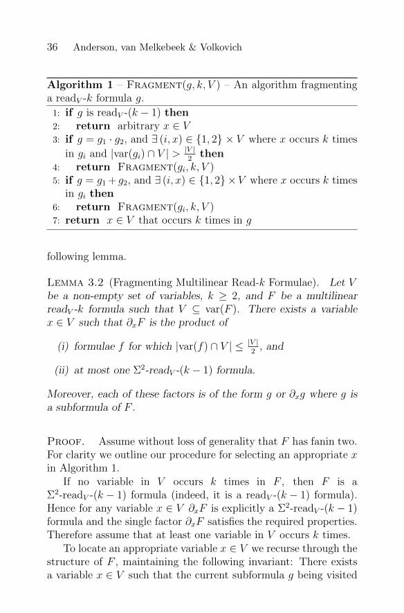
Algorithm 1 – Fragment(g, k, V ) – An algorithm fragmentinga readV -k formula g.
1: if g is readV -(k − 1) then2: return arbitrary x ∈ V3: if g = g1 · g2, and ∃ (i, x) ∈ 1, 2 × V where x occurs k times
in gi and |var(gi) ∩ V | > |V |2
then4: return Fragment(gi, k, V )5: if g = g1 + g2, and ∃ (i, x) ∈ 1, 2 ×V where x occurs k times
in gi then6: return Fragment(gi, k, V )7: return x ∈ V that occurs k times in g
following lemma.
Lemma 3.2 (Fragmenting Multilinear Read-k Formulae). Let Vbe a non-empty set of variables, k ≥ 2, and F be a multilinearreadV -k formula such that V ⊆ var(F ). There exists a variablex ∈ V such that ∂xF is the product of
(i) formulae f for which |var(f) ∩ V | ≤ |V |2
, and
(ii) at most one Σ2-readV -(k − 1) formula.
Moreover, each of these factors is of the form g or ∂xg where g isa subformula of F .
Proof. Assume without loss of generality that F has fanin two.For clarity we outline our procedure for selecting an appropriate xin Algorithm 1.
If no variable in V occurs k times in F , then F is aΣ2-readV -(k − 1) formula (indeed, it is a readV -(k − 1) formula).Hence for any variable x ∈ V ∂xF is explicitly a Σ2-readV -(k − 1)formula and the single factor ∂xF satisfies the required properties.Therefore assume that at least one variable in V occurs k times.
To locate an appropriate variable x ∈ V we recurse through thestructure of F , maintaining the following invariant: There existsa variable x ∈ V such that the current subformula g being visited

PIT for Multilinear Bounded-Read Formulae 37
contains all k occurrences of x in F . Setting g to be F satisfiesthis invariant initially.
If the top gate of g is a multiplication gate, recurse on the childthat depends on more than |V |
2of the variables in V and contains
k occurrences of some variable in V . If no such child exists, endthe recursion at g and select a variable from V that occurs k timesin g. Such a variable must exist by the invariant.
If the top gate of g is an addition gate, g = g1 +g2, and at leastone of its children, gi, has a variable in V that occurs k times ingi, recurse on gi. Otherwise, both children of g are readV -(k − 1)formulae. Select a variable from V that occurs k times in g endingthe recursion. Again, such a variable must exist by the invariant.
Let x ∈ V be the variable selected by the procedure. We arguethat ∂xF can be written in the desired form. Denote by f thesubformula where the recursion ended. Since f contains all theoccurrences of x in F , Proposition 2.4 tells us that ∂xF = ∂xf ·∏
g∈UF (f) g, where UF (f) denotes the unvisited multiplication gateson the path from the root of F to f . By the selection rule formultiplication gates, all the gates g ∈ UF (f) each depend on at
most |V |2
variables from V . All that remains is to analyze ∂xf .There are two cases depending on the top gate of f .
Suppose the top gate of f is a multiplication gate: f = f1 · f2.Without loss of generality assume that x ∈ var(f1). Since F ismultilinear, we can write
(3.3) ∂xf = (∂xf1) · f2.
The stopping rule and multilinearity together imply that f1 (and
hence ∂xf1 depends on at most |V |2
of the variables in V , and thatf2 either:
(i) depends on at most |V |2
of the variables in V , or
(ii) does not contain k occurrences of any variable in V and there-fore is a Σ2-readV -(k − 1) formula.
In either case, the resulting factoring of ∂xF satisfies the propertiesin the statement of the lemma.

38 Anderson, van Melkebeek & Volkovich
Suppose the top gate of f is an addition gate: f = f1 + f2.According to the stopping rule both children of f are readV -(k − 1)formulae, making f a Σ2-readV -(k − 1) formula, and so is ∂xf .The resulting factoring of ∂xF again satisfies the properties in thestatement of the lemma.
For the case k = 1 the proof of Lemma 3.2 yields the unweightedversion of Lemma 3.1.
3.3. Fragmenting Sparse-Substituted Formulae. In thissubsection we extend our fragmenting arguments to work forsparse-substituted formulae.
First consider a multilinear sparse-substituted read-once for-mula F . The idea is to apply the argument from Lemma 3.1 andthe chain rule to locate a variable x such that ∂xF is almost frag-mented. By this we mean that each of the factors of ∂xF dependson at most half of the variables except the factor that was originallya sparse polynomial that depends on x. The sparse polynomial,say f , may depend on too many variables. In that case we performfurther operations so that f factors into smaller pieces. Through asequence of partial derivatives and zero-substitutions we eliminateall but one term in f . This implies that the sparse polynomial andhence the overall resulting formula F ′ is 1
2-split. To perform the
additional step, observe that for any variable x, either at most halfof the terms in f depend on x or at most half do not. In the formercase, taking the partial derivative with respect to x eliminates atleast half of the terms; setting x to 0 has the same effect in the lat-ter case. Repeating this process a number of times logarithmic inthe maximum number of terms eliminates all but one of the terms,resulting in a trivially split formula.
This is the intuition behind the sparse-substituted extension ofLemma 3.1 and corresponds to the first part of the next lemma.The second part is the sparse-substituted extension of Lemma 3.2and follows from that lemma by a simple observation.
Lemma 3.4 (Fragmentation Lemma). Let V be a non-emptyset of variables, k ≥ 1, and F be a multilinear sparse-substitutedreadV -k formula such that V ⊆ var(F ). Let t denote the maximum
PIT for Multilinear Bounded-Read Formulae 39
number of terms in each substituted polynomial.
(i) If k = 1, there exist disjoint sets of variables P,Z with|P ∪ Z| ≤ log(t) + 1 such that ∂PF |Z←0 is non-zero and is a
product of factors f for which |var(f) ∩ V | ≤ |V |2
. Moreover,the factors are subformulae of F .
(ii) If k ≥ 2, there exists a variable x ∈ V such that ∂xF is theproduct of
(a) formulae f for which |var(f) ∩ V | ≤ |V |2
, and
(b) at most one Σ2-readV -(k − 1) formula.
Moreover, each of these factors is of the form g or ∂xg whereg is a subformula of F .
Proof. We argue the two parts separately.
Part 1. Assume without loss of generality that F has fanin two.Write F = B(ρ1, . . . , ρr) as in Definition 2.3, where B ∈ F[Y ]
is the backbone of F and the ρi’s are t-sparse multilinear poly-nomials. Define Y ′
.= yi ∈ Y | |var(ρi) ∩ V | > 0 and the weight
function w : Y ′ → N by yi 7→ |var(ρi) ∩ V |. Because F is a readV -once formula and V ⊆ var(F ), W
.=∑
y∈Y ′ w(y) = |V |. ApplyLemma 3.1 to B with set Y ′ and weight function w to determinea variable yi ∈ Y ′ ⊆ Y such that we can write ∂yiB =
∏j bj where
the bj’s are subformulae of B and∑
y∈var(bj) w(y) ≤ W2
= |V |2
. Pick
x ∈ var(ρi) ∩ V . Note that x exists because i ∈ Y ′. Since F is areadV -once formula, only ρi depends on x and applying the chainrule produces
∂xF = ∂xB(ρ1, . . . , ρr) = (∂xρi) · (∂yiB(y1, . . . , yr))|Y←ρ= (∂xρi) ·
∏jgj
where gj.= bj|Y←ρ. Observe that each gj is a subformula of F and
depends on at most |V |2
variables from V . If ∂xρi depends on at
most |V |2
of the variables in V , the lemma is complete with P.= x
and Z.= ∅. Therefore, assume otherwise.
Let ρ.= ∂xρi. Write ρ =
∑`j=1Mj where ` ≤ t and each Mj is
a distinct term.

40 Anderson, van Melkebeek & Volkovich
Claim 3.5. There exist disjoint P ′, Z ⊆ var(ρ) such that|P ′ ∪ Z| ≤ log ` and ∂P ′ρ|Z←0 is a single term.
Proof. We proceed by induction on `. In the base case ` = 1.Trivially, ρ is a term. It suffices to set P ′ = Z = ∅ and hence|P ′ ∪ Z| = 0 = log 1.
In the induction step ` > 1, there is a variable z ∈ var(ρ)that divides some term Mj of ρ, but not all terms of ρ. To seethis, suppose that each variable in var(ρ) divides each term of ρ,then, because ρ is multilinear, each term must be the same, so` = 1. This contradicts ` > 1. We complete by considering twocases based on the number of terms that z divides. Suppose zdivides at most `
2terms of ρ. Then ∂zρ has at most `
2terms and is
non-zero. By induction there are sets P ′′, Z ′ ⊆ var(∂zρ) ⊆ var(ρ)with |P ′′ ∪ Z ′| ≤ log `
2= (log `) − 1 such that ∂P ′′∂zρ|Z′←0 is a
single term. Set P ′.= P ′′ ∪ z and Z
.= Z ′ to conclude this
case. Otherwise, z divides more than `2
terms of ρ, but not all ofthem. Thus ρ|z←0 has at most `
2terms and is non-zero. Applying
the induction hypothesis to ρ|z←0 suffices to conclude as in theprevious case but setting P ′
.= P ′′ and Z
.= Z ′ ∪ x.
Apply Claim 3.5 to ρ to get P ′∪Z ⊆ var(ρ) with |P ′∪Z| ≤ log t.Set P
.= P ′ ∪ x. Note that ∂PF |Z←0 = (∂Pρi|Z←0) ·∏j gj 6≡ 0,
because F is multilinear, P∪Z ⊆ var(ρ), and ∂Pρi|Z←0 is a non-zeroterm. Finally, observe that because ∂Pρi|Z←0 is a term it triviallyfactors into a product of subformulae of F (namely variables) thateach depend on at most one variables in V . We conclude by notingthat 1 ≤ |V |
2. This follows because ρi depends on x ∈ V and at
least one other variable in V (since ∂xρi depends on more than |V |2
variables in V other than x), hence |V | ≥ 2.
Part 2. Here the proof is essentially the same as the proof ofLemma 3.2. Since k ≥ 2, the argument always halts at an internalgate and never reaches a sparse-substituted input. Only the num-ber of occurrences of each variable is relevant to the decisions theargument makes. This implies that the argument does not changewhen sparse-substituted formulae are considered (and is even in-dependent of the sparsity parameter). Thus, this part of the proofis immediate as a corollary to the proof of Lemma 3.2.
PIT for Multilinear Bounded-Read Formulae 41
Observe that the cost of applying the Fragmentation Lemmato a read-once formula is log(t) + 1 partial derivatives and zero-substitutions, whereas applying it to a formula that is not read-once requires only a single partial derivative (though the promisedresult is weaker in this case).
It is useful to have a version of Part 2 of the FragmentationLemma generalized to structurally-multilinear formulae. The ar-gument is the same as for the earlier version except that in additionto selecting an appropriate x, we must pick an α ∈ F, such that∂x,αF
.= F |x←α − F |x←0 is non-zero. The directed partial deriva-
tive comes in here because ∂xF.= F |x←1−F |x←0 may be zero even
when F depends on x, because F is not multilinear.
Lemma 3.6 (Fragmentation Lemma for Structurally-MultilinearFormulae). Let V be a non-empty set of variables, k ≥ 2, andF be a structurally-multilinear sparse-substituted readV -k formulawith V ⊆ var(F ). Let t denote the maximum number of terms ineach substituted polynomial. There exists a variable x ∈ V andα ∈ F such that ∂x,αF is non-zero and the product of
(i) formulae f for which |var(f) ∩ V | ≤ |V |2
, and
(ii) at most one Σ2-readV -(k − 1) formula.
Moreover, each of these factors is of the form g or ∂xg where g isa subformula of F .
Proof. Repeat the proof of Lemma 3.4, Part 2, but add thefollowing step. After selecting an appropriate variable x that Fdepends on, select an α such that ∂x,αF 6≡ 0. By the Schwartz-Zippel Lemma, such an α exists within the algebraic closure F ofF. Note that, in fact, if |F| is larger than the degree of x in F suchan α is present in F.
3.4. Shattering Multilinear Formulae. The previous sub-sections establish a method for fragmenting multilinear sparse-substituted read-k formulae. We now apply the FragmentationLemma (Lemma 3.4) to simultaneously split all branches of a mul-tilinear sparse-substituted Σm-read-k formula. We call this pro-cess shattering. When k = 1, applying the Fragmentation Lemma

42 Anderson, van Melkebeek & Volkovich
greedily to a factor of a branch that depends on the largest num-ber of variables suffices to split a multilinear sparse-substitutedΣm-read-once formula to an arbitrary level. To obtain an α-splitformula in the end, we need O(m (log(t)+1)
α) partial derivatives and
zero-substitutions.In the case of arbitrary read-value k > 1 the Fragmentation
Lemma is not immediately sufficient for the task. As in the read-once case, we can apply the lemma greedily to a largest factor of aread-k branch to α-split the branch within at most 2
αapplications.
However, this is assuming that Case (ii.b) of the FragmentationLemma never occurs where the Σ2-read-(k − 1) factor depends onmore than half (possibly all) of the variables. When this case occursthe fragmentation process fails to split the formula into pieces eachdepending on few variables. To resolve the issue, we leverage thefact that this troublesome factor is both large and a Σ2-read-(k−1)formula.
Consider a read-k formula F on n variables. Apply the Frag-mentation Lemma to F . Suppose that Case (ii.b) of the lemmaoccurs, producing a variable x, and that the corresponding Σ2-read-(k − 1) factor of ∂xF depends on more than n
2of the vari-
ables. Without loss of generality, ∂xF = H · (H1 + H2), whereH is a product of read-k formulae each depending on at most n
2
variables, and both H1 and H2 are read-(k− 1) formulae. RewriteF by distributing the top level multiplication over addition:
F ′.= (H ·H1) + (H ·H2) ≡ H · (H1 +H2) = ∂xF.
Let V.= var(H1 +H2). F ′ is explicitly a Σ2-readV -(k− 1) formula
and a readV -k formula. However, F ′ is almost certainly not a read-k formula. Partition the variables into “same-read” sets, that is,sets of variables that appear the exact same number of times. Byfurther restricting to the largest “same-read” set of variables inthe larger of the two subformulae H1 and H2, we can argue theexistence of a subset V ′ ⊆ V that contains at least a 1
2kfraction of
the variables in V such that the read of H1 and H2 with respect toV ′ sum to at most k. Note that prior to this restriction the upperbound on this sum is 2(k − 1). This action effectively breaks upthe original formula F into two branches without increasing the
PIT for Multilinear Bounded-Read Formulae 43
sum of the read values of the branches. Since |V | ≥ n2, the set V ′
is at most a factor 4k smaller than n, and the number of branchesincreased by one.
This operation can be performed at most k − 1 times on aread-k formula before either: (i) the attempted greedy splittingis successful, or (ii) the formula becomes the sum of k read-onceformulae with respect to some subset V of [n]. In the latter casewe are effectively in the situation we first described with k = 1,and all subsequent splittings will succeed. In either case we obtaina formula that is shattered with respect to a subset V that is atmost a factor kO(k) smaller than n.
In summary, the Shattering Lemma splits multilinear sparse-substituted Σm-read-k formulae to an arbitrary extent, albeit withsome restriction of the variable set and an increase in top fanin.Moreover, each of the branches in the shattered formula are presentin the original input formula, either as such or after taking somepartial derivatives and zero-substitutions. This technical propertyfollows from the properties of the Fragmentation Lemma and willbe needed in the eventual application.
Lemma 3.7 (Shattering Lemma). Let α : N → (0, 1] be a non-increasing function. Let F ∈ F[x1, . . . , xn] be a formula of theform F = c +
∑mi=1 Fi, where c is a constant, and each Fi is a
non-constant multilinear sparse-substituted read-ki formula. Let tdenote the maximum number of terms in each substituted polyno-mial. There exist disjoint subsets P,Z, V ⊆ [n] such that ∂PF |Z←0
can be written as c′ +∑m′
i=1 F′i , where c′ is a constant, and
m′ ≤ k.=∑m
i=1 ki,
each F ′i is multilinear and α(m′ + 2)-splitV ,
|P ∪ Z| ≤ (k −m+ 1) · 4kα(k+2)
· (log(t) + 1), and
|V | ≥(α(k+2)
8k
)k−m· n− 8k
α(k+2)· (log(t) + 1).
Moreover, the factors of each of the F ′i ’s are of the form ∂Pf |Z←0,where f is some subformula of some Fj and P ⊆ P .
44 Anderson, van Melkebeek & Volkovich
Proof. We iteratively construct disjoint subsets P,Z, V ⊆ [n],maintaining the invariant that ∂PF |Z←0 can be written as
F ′.= c′ +
∑m′
i=1 F′i where
(1) each F ′i is a readV -k′i formula and c′ is a constant
(2) m′ ≤ k
(3)∑m′
i=1 k′i.= k′ ≤ k
(4) each F ′i is the product of factors of the form ∂Pf |Z←0 where fis some subformula of some Fj and P ⊆ P .
Setting P ← ∅, Z ← ∅, V ← [n] and F ′ ← F realizes theinvariant initially. The fact that m′ ≤ k follows because each Fi isnon-constant.
The goal of our algorithm is to α(m′ + 2)-splitV the formulaF ′. Each iteration (but the last) consists of two phases: a split-ting phase, and a rewriting phase. In the splitting phase we at-tempt to split F ′ by greedily applying the Fragmentation Lemma(Lemma 3.4) on each of the branches F ′i . The splitting phase mayget stuck because of a Σ2-readV -(k′i − 1) subformula that blocksfurther splitting. If not and the resulting F ′ is sufficiently split,the algorithm halts. Otherwise, the algorithm enters the rewritingphase where it expands the subformula that blocked the Fragmen-tation Lemma and reasserts the invariant, after which the nextiteration starts. A potential argument shows that the number ofiterations until a successful splitting phase is bounded by k −m.We first describe the splitting and rewriting phases in more detail,then argue termination and analyze what bounds we obtain for thesizes of the sets P , Z, and V .
Splitting. Assume that F ′ is not α(m′+2)2
-splitV , otherwise halt. LetF ′ij be a subformula of F ′ that depends on the most variables in Vout of all the factors of the F ′i ’s. Apply the Fragmentation Lemma(Lemma 3.4) with respect to the set V ∩ var(F ′ij) to produce setsP ′, Z ′ ⊆ [n]. Since F ′ is multilinear, the Fragmentation Lemmaimplies one of the following holds:

PIT for Multilinear Bounded-Read Formulae 45
(i) The factors of ∂P ′F′ij|Z′←0 depend on at most
|V ∩var(F ′ij)|2
vari-ables in V ∩ var(F ′ij), or
(ii) ∂P ′F′ij|Z′←0 has one multilinear sparse-substituted Σ2-readV -
(k′i − 1) factor which depends on more than|V ∩var(F ′ij)|
2vari-
ables in V ∩ var(F ′ij).
Repeatedly perform this greedy application, adding elements tothe sets P ′ and Z ′ until either case (ii) above occurs or ∂P ′F
′|Z′←0
is α(m′+2)2
-splitV . In the former case we start a rewriting phaseand modify ∂P ′F
′|Z′←0 before we re-attempt to split. In the latter
case our goal has been achieved provided that |P ′ ∪ Z ′| ≤ |V |2
:We can add P ′ to the set P we already had, similarly add Z ′
to Z, and replace V by V ′.= V \ (P ′ ∪ Z ′). The assumption
that |P ′ ∪ Z ′| ≤ |V |2
guarantees that |V ′| ≥ |V |2
. Since ∂PF |Z←0
(which equals ∂P ′F′|Z′←0) is α(m′+2)
2-splitV , the latter inequality
implies that the formula is α(m′ + 2)-splitV ′ . If the assumption
that |P ′ ∪ Z ′| ≤ |V |2
does not hold, then outputting V ′ = ∅ willmeet the size bound for that set and trivially make the formula∂PF |Z←0 α(m′ + 2)-splitV ′ .
The splitting phase maintains the invariant. Regarding Part (4)of the invariant, observe that the factors produced by the Fragmen-tation Lemma are subformulae of the input to the FragmentationLemma (for which the invariant initially held).
Rewriting. We now describe the rewriting phase. Consider the setof variables V at the beginning of the preceding splitting phase.Let F ′ij be the subformula the splitting phase blocked on, andlet H1 and H2 denote the two branches of the multilinear sparse-substituted Σ2-readV -(k′i − 1) subformula of ∂xF
′i that caused the
blocking Case (ii.b) of the Fragmentation Lemma to happen. Wehave that ∂P ′F
′ij|Z′←0 = H · (H1 + H2), where H is some readV -k′i
formula that is independent of the variables in V ∩ var(H1 + H2).Let V ′
.= V ∩ var(H1 + H2). Partition V ′ into sets V ′0 , ..., V ′k′i−1
based on the exact number of occurrences of each variable in H1.Let V ′′ be any set from this partitioning excluding the set V ′0 (wewill restrict the choice of V ′′ later). This implies that H1 is readV ′′-

46 Anderson, van Melkebeek & Volkovich
k′i1 and H2 is readV ′′-k′i2 for some integers k′i1 and k′i2 such that
k′i1, k′i2 < k′i and k′i1 + k′i2 ≤ k′i.
Rewrite ∂P ′F′|Z′←0 as a top fanin m′+2 formula by distributing
multiplication over addition in the term ∂P ′F′i |Z′←0:
(3.8) ∂P ′F′|Z′←0 ≡ (H ·H1) + (H ·H2) +
∑j 6=i
∂P ′F′j|Z′←0.
Observe that∑
j 6=i ∂P ′F′j|Z′←0 is a readV ′′-(
∑j 6=i k
′j) formula as
partial derivatives and substitutions do not increase the read-value,and V ′′ ⊆ V . The term (H ·H1) + (H ·H2) may not be a readV -k′iformula, but it must be a readV ′-k
′i formula. It is explicitly the
sum of a readV ′′-k′i1 formula and a readV ′′-k
′i2 formula for some
k′i1, k′i2 < k′i with k′i1 + k′i2 ≤ k′i. The representation of ∂P ′F
′|Z′←0
in Equation (3.8) is therefore a readV ′′-k′ formula with top fanin
m′ + 2.Set F ′ to be this representation of ∂P ′F
′|Z′←0. Merge branchesthat have become constant into a single constant branch. Thismaintains the invariant that m′ ≤ k′ ≤ k. Setting V ← V ′′ makesF ′ a top-fanin-(m′ + 1) readV -k′ formula. As for Part (4) of theinvariant, note that the subformula F ′ij which blocked the Frag-mentation Lemma originally satisfied it during the splitting phase.This means that with respect to the additional partial derivativesand zero-substitutions performed for the attempted split, H1 andH2, as well as H, satisfy the invariant as new factors of the branchesF ′i . Thus, the new F ′ satisfies the full invariant. This completesthe rewriting phase and one full iteration of the algorithm.
Correctness. We repeat the sequence of splitting and rewritingphases until a splitting phase runs till completion. In that case thealgorithm produces disjoint sets P,Z, V ⊆ [n] such that ∂PF |Z←0
can be written as a α(m′+2)-splitV formula with top fanin m′+1 ≤k + 1.
Apart from the size bounds on the sets P , Z, and V , all thatremains to establish correctness is termination. To argue the latterwe use the following potential argument. Consider the sum
∑m′
i=1 k′i
and view it as m′ blocks of integer size, where k′i is the size of theith block. Over the course of the algorithm blocks can only staythe same, shrink, or be split in a nontrivial way. The latter is

PIT for Multilinear Bounded-Read Formulae 47
what happens in a rewriting phase. As soon as all blocks are ofsize at most 1, the splitting phase is guaranteed to run successfullybecause Case (ii.b) of the Fragmentation Lemma cannot occur forread-once formulae, and the algorithm terminates. As we start outwith m nontrivial blocks and a value of k for the sum, there canbe no more than k −m nontrivial splits. Therefore, there are nomore than k−m rewriting phases and k−m+ 1 splitting phases.
Analysis. We now bound the size of P ∪ Z. We first analyze howmany times the Fragmentation Lemma is applied in each split-ting phase. The goal is to α(m′+2)
2-splitV each of the m′ branches.
To α(m′+2)2
-splitV one branch, 4α(m′+2)
applications of the Frag-mentation Lemma are sufficient, since each application reducesthe intersection of the factors with V to at most half the orig-inal amount. Since the invariant maintains m′ ≤ k and α isnon-increasing, we can upper bound the number of applicationsof the Fragmentation Lemma during an arbitrary iteration by
4m′
α(m′+2)≤ 4k
α(k+2). Each single application of the Fragmentation
Lemma adds at most (log(t) + 1) variables to P ′ and Z ′. Sincethere are at most k −m + 1 splitting phases, across all iterationsat most (k−m+ 1)(log(t) + 1) 4k
α(k+2)variables are added to P ∪Z.
We finish by lower bounding the size of V . Consider the changein |V | over one combined splitting/rewriting iteration. We have
that |V ′| ≥ α(m′+2)4|V |, because F ′ was not α(m′+2)
2-splitV before
attempting to split F ′ij (so the largest number of variables in V
that a factor depends on is at least α(m′+2)2· |V |), F ′ij was chosen
for its maximal dependence on variables from V , and |var(H1 +H2) ∩ V | ≥ |var(F ′ij) ∩ V |/2. If we pick V ′′ to be the largestset from the partitioning V ′0 , V ′1 , ..., V ′k′i−1 excluding V ′0 , and we
assume without loss of generality that |var(H1)| ≥ |var(H2)|, wehave that |V ′′| ≥ 1
2(k′i−1)|V ′|. Combining these inequalities and
using the facts that α is non-increasing and k ≥ k′i,m′ gives:
|V ′′| ≥ 1
2(k′i − 1)|V ′| ≥ α(m′ + 2)
8(k′i − 1)|V | ≥ α(k + 2)
8k|V |.
This means that |V | decreases by a factor of at most 8kα(k+2)
in
each combined splitting/rewriting iteration. At the end of the final

48 Anderson, van Melkebeek & Volkovich
splitting phase |V ′| ≥ |V |−2|P ′∪Z ′| because V ′ is set to the empty
set when |P ′ ∪ Z ′| ≥ |V |2
. Recall that |P ′ ∪ Z ′| ≤ 4kα(k+2)
(log(t) +
1). Since there are at most k − m combined splitting/rewritingiterations, this gives the following lower bound at the end:
|V | ≥(α(k + 2)
8k
)k−m· n− 8k
α(k + 2)· (log(t) + 1).
4. Reducing Testing Read-(k + 1)Formulae toTesting Σ2-Read-k Formulae
In this section we describe two methods of reducing identity test-ing structurally-multilinear sparse-substituted read-(k + 1) formu-lae to identity testing structurally-multilinear sparse-substitutedΣ2-read-k formulae. The first reduction is non-blackbox and is el-ementary. The second reduction is blackbox and makes use of theFragmentation Lemma of the preceding section.
4.1. Non-Blackbox Reduction. In the non-blackbox set-ting we only need to deal with multilinear sparse-substitutedformulae, because we can efficiently transform structurally-multilinear sparse-substituted read-k formulae into multilinearsparse-substituted read-k formulae in a non-blackbox way whilepreserving non-zeroness using the transformation L from Sec-tion 2.1.4 (see Definition 2.7). Recall Section 1.2.2 for the intuitionbehind the following non-blackbox reduction from identity test-ing multilinear sparse-substituted read-(k+1) formulae to identitytesting multilinear sparse-substituted Σ2-read-k formulae.
Lemma 4.1 (Read-(k+1) PIT ≤ Σ2-Read-k PIT – Non-BlackboxMultilinear). For an integer k ≥ 0, given a deterministic iden-tity test for n-variate size-s multilinear sparse-substituted Σ2-read-k formulae that runs in time T (k, n, s, t), where t denotes themaximum number of terms in each substituted polynomial, thereis a deterministic algorithm that tests n-variate size-s multilin-ear sparse-substituted read-(k + 1) formulae that runs in timeO((k + 1)n · T (k, n, s, t) + poly(s)).
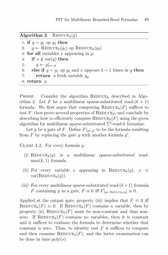
PIT for Multilinear Bounded-Read Formulae 49
Algorithm 2 – Reducek(g)
1: if g = g1 op g2 then2: g ← Reducek(g1) op Reducek(g2)3: for all variables x appearing in g:4: if x 6∈ var(g) then5: g ← g|x←0
6: else if g = g1 op g2 and x appears k + 1 times in g then7: return a fresh variable yg8: return g
Proof. Consider the algorithm Reducek described in Algo-rithm 2. Let F be a multilinear sparse-substituted read-(k + 1)formula. We first argue that computing Reducek(F ) suffices totest F , then prove several properties of Reducek, and conclude bydescribing how to efficiently compute Reducek(F ) using the givenalgorithm for multilinear sparse-substituted Σ2-read-k formulae.
Let g be a gate of F . Define F |g←g′ to be the formula resultingfrom F by replacing the gate g with another formula g′.
Claim 4.2. For every formula g:
(i) Reducek(g) is a multilinear sparse-substituted read-max(k, 1) formula.
(ii) For every variable x appearing in Reducek(g), x ∈var(Reducek(g)).
(iii) For every multilinear sparse-substituted read-(k+1) formulaF containing g as a gate, F ≡ 0 iff F |g←Reducek(g) ≡ 0.
Applied at the output gate, property (iii) implies that F ≡ 0 iffReducek(F ) ≡ 0. If Reducek(F ) contains a variable, then byproperty (ii) Reducek(F ) must be non-constant and thus non-zero. If Reducek(F ) contains no variables, then it is constantand it suffices to evaluate the formula to determine whether thatconstant is zero. Thus, to identity test F it suffices to computeand then examine Reducek(F ), and the latter examination canbe done in time poly(s).

50 Anderson, van Melkebeek & Volkovich
We argue Claim 4.2 by structural induction on g. In the basecase, g is a sparse-substituted input. Property (i) holds as thesparse-substituted inputs are defined to be read-once. Property(ii) holds because the only action of Reducek is to eliminate allvariables that g does not depend on. It immediately follows thatF ≡ F |g←Reducek(g) and property (iii) holds.
In the induction step, g = g1 op g2 for op ∈ +,×.Applying the induction hypothesis twice we have that F ≡0 iff F |g1←Reducek(g1) ≡ 0 iff
(F |g1←Reducek(g1))|g2←Reducek(g2)
≡ F |g←(Reducek(g1) op Reducek(g2)) ≡ 0.
There are two cases.
1. After reducing the children of g, there is a variable x ∈ var(g)that appears k + 1 times in g.
In that case, Reducek(g) returns yg. Since yg is a read-onceformula, properties (i) and (ii) are immediate. We now argueproperty (iii), i.e., that F ≡ 0 iff F |g←yg ≡ 0.
Since F is a read-(k + 1) formula, g must contain every oc-currence of x. Thus F |g←yg does not depend on x. As ygoccurs only once in F |g←yg , without loss of generality, write:F |g←yg ≡ P + Q · yg, for two polynomials P and Q that donot depend on x or yg. If Q ≡ 0, then F is independent of g,so F |g←yg ≡ F . If Q 6≡ 0, then F is non-zero because Q · gdepends on x but P does not, and F |g←yg 6≡ 0 for a similarreason. In both cases we conclude that F ≡ 0 iff F |g←yg ≡ 0and property (iii) holds.
2. After reducing the children every variable x ∈ var(g) occursat most k times in g.
In this case, Reducek(g) is explicitly a read-k formula andproperty (i) holds. Properties (ii) and (iii) hold because theloop eliminates each variable x 6∈ var(g) that occurs in gwhile not changing the polynomial computed at g.

PIT for Multilinear Bounded-Read Formulae 51
This finishes the proof of Claim 4.2. The correctness of theoverall algorithm follows by applying Claim 4.2 with g = F .
It remains to argue that Reducek(F ) can be efficiently com-puted. An inspection of Reducek shows that it does not increasethe size, number variables, or sparsity of gates it transforms. Themain difficulty is implementing the test x 6∈ var(g) from Line 4.
1. When g is a sparse polynomial, x 6∈ var(g) can be decided inpoly(s) time by summing coefficients of identical terms in g’slist of monomials to aggregate duplicates and then searchingfor a monomial with non-zero coefficient in which x appears.
2. Otherwise g is an internal gate. Property (ii) for the reducedchildren of g implies that they depend on exactly those vari-ables that occur in them.
(a) When g is a multiplication gate and both reduced chil-dren of g contain variables, g depends on exactly thosevariables that appear in g and hence the test in Line 4is always false. When g is a multiplication gate and atleast one reduced child contains no variables, determinethe constant value of those children. If a constant childevaluates to zero, g ≡ 0 and the test in Line 4 is alwaystrue, otherwise it is always false. Thus when g is a mul-tiplication gate, x 6∈ var(g) can be decided in poly(s)time.
(b) When g is an addition gate and at least one reducedchild of g does not contain x, no additional work isneeded as the dependence on x cannot change at g andhence the test in Line 4 is false.
Otherwise, both reduced children of g contain x. In thatcase we decide x 6∈ var(g) by taking the partial deriva-tive of each reduced child with respect to the variablex and then applying the assumed identity test on Σ2-read-k formulae to test whether ∂g
∂x6≡ 0. Note that ∂g
∂xis
indeed a Σ2-read-k formula as property (i) implies thatthe reduced children are read-k formulae. The partialderivative can be computed in time poly(s) since the

52 Anderson, van Melkebeek & Volkovich
multiplication gates in the multilinear subformulae ofthe reduced children are variable disjoint by property(ii).
Since F is a read-(k + 1) formula, for any given variable x, thenontrivial case in 2b) can happen at most k + 1 times. Moreover,for that case to happen x has to be one of the variables of theoriginal formula F . This implies that Reducek(F ) makes at most(k+ 1)n calls to the Σ2-read-k identity test. All the other work toevaluate Line 4 is poly(s). Combining the cost for evaluating Line4 with a straight-forward implementation of the rest of Reducek,we conclude that our identity test runs in time claimed.
Since testing multilinear sparse-substituted read-k formulae istrivial for k = 0, the special case of Lemma 4.1 with k = 0 yieldsthe following corollary.
Corollary 4.3. There is a deterministic algorithm for identitytesting multilinear sparse-substituted read-once formulae that runsin time poly(s), where s denotes the size of the formula.
In fact, the proof of Lemma 4.1 for k = 0 shows that Corol-lary 4.3 even holds without the multilinearity condition (which isnon-vacuous for sparse-substituted formulae), but we will not needthat extension.
4.2. Blackbox Reduction. Let F be a structurally-multilinearread-(k + 1) formula. We construct a generator for F using a gen-erator G for structurally-multilinear Σ2-read-k formulae. If F is aread-k formula, the assumed generator alone suffices. Otherwise,we apply the Fragmentation Lemma for structurally-multilinearsparse-substituted formulae (Lemma 3.6) to show that there is apartial derivative of F that has mostly small factors and, possibly,one factor that is a large structurally-multilinear Σ2-read-k for-mula. In the former case the factors are small enough to be hit re-cursively, and in the latter case the factor is hit by the assumed gen-erator for structurally-multilinear Σ2-read-k formulae. The proper-ties of the SV-generator (Proposition 2.12 and Lemma 2.14) implythat if Gn is a generator for the partial derivative of a polynomial

PIT for Multilinear Bounded-Read Formulae 53
with n variables, then Gn + Gn,1 is a generator for the originalpolynomial.
Lemma 4.4 (Read-(k + 1) PIT ≤ Σ2-Read-k PIT – BlackboxStructurally-Multilinear). For an integer k ≥ 1, let G be a gen-erator for n-variate structurally-multilinear sparse-substituted Σ2-read-k formulae, and let F be a non-zero n-variable structurally-multilinear sparse-substituted read-(k + 1) formula. Then G +Gn,log |var(F )| hits F .
Proof. First observe that if F is read-k, we are immediatelydone because F (G) 6≡ 0 and 0 is in the image of the SV-generator(by Proposition 2.12, Part (i)).
The proof goes by induction on |var(F )|. If |var(F )| = 0, thelemma holds trivially as F is constant. If |var(F )| = 1, F is aread-once formula, which is covered by the above observation. Forthe induction step, by the above observation we can assume that Fis read-(k + 1) and not read-k. Therefore, F meets the conditionsto apply the structurally-multilinear version of the FragmentationLemma (Lemma 3.6) with V = var(F ). The lemma produces avariable x ∈ var(F ) and α ∈ F. The factors of ∂x,αF all de-
pend on at most |var(F )|2
variables and are read-(k + 1) formulae,except for at most one which is a Σ2-read-k formula. The induc-tion hypothesis gives that the former factors of ∂x,αF are all hitby G + Gn,log(|var(F )|/2). The latter factor (if it occurs) is hit by G.Applying Lemma 2.14 gives that G +Gn,log(|var(F )|/2) +Gn,1 hits F .Recalling Proposition 2.12, Part (iii), implies that G +Gn,log |var(F )|hits F .
5. Reducing Testing Σ2-Read-k Formulae toTesting Read-k Formulae
In this section we present two methods of reducing identity testingstructurally-multilinear sparse-substituted Σ2-read-k formulae toidentity testing structurally-multilinear sparse-substituted read-kformulae. We first develop those methods for multilinear ratherthan structurally-multilinear sparse-substituted formulae, and thenshow how to lift them to the latter setting.
54 Anderson, van Melkebeek & Volkovich
Both reductions rely on a common theorem (Theorem 5.4),which we prove in Section 5.2. Informally, that theorem says thatfor a non-zero multilinear sparse-substituted Σ2-read-k formula Fon n variables and a shift σ satisfying some simple conditions, theshifted formula F (x + σ) is hit by the SV-generator Gn,w withw = kO(k)(log(t) + 1), where t denotes the maximum number ofterms in each substituted polynomial.
Note that, since F is a non-zero polynomial, such a theorem istrivially true for a typical shift σ, even with w = 0. The interestingpart of the theorem is the simplicity of the conditions on σ thatguarantee the hitting property. In particular, the properties neededof σ allow such a σ to be computed efficiently either by an identitytest for multilinear sparse-substituted read-k formulae, or as anelement in the image of a hitting set generator for such formulae.
In Section 5.1 we argue that small sums of specially shiftedmultilinear sparse-substituted read-k formulae cannot compute aterm of high degree. This is the Key Lemma for multilinear sparse-substituted formulae and is a formalization of Lemma 1.3 from theintroduction. Using the Key Lemma and the hitting property ofthe SV-generator (Lemma 2.17), we prove (as Theorem 5.4 in Sec-tion 5.2) that the SV-generator hits small sums of specially shiftedmultilinear sparse-substituted read-k formulae. In Section 5.3 andSection 5.4 we use Theorem 5.4 to argue reductions from identitytesting multilinear sparse-substituted Σ2-read-k formula to iden-tity testing multilinear sparse-substituted read-k formulae in boththe non-blackbox and blackbox settings.
Section 5.4 concludes by extending the blackbox reduction tostructurally-multilinear sparse-substituted read-k formulae. To dothis we use the transformation L from Section 2.1.4 (see Defini-tion 2.7) to generalize the Key Lemma to structurally-multilinearsparse-substituted formulae, and then argue how the other ingre-dients transfer. The corresponding step in the non-blackbox set-ting is straightforward because there L can be directly applied toefficiently reduce the problem of testing structurally-multilinearsparse-substituted read-k formulae to testing multilinear sparse-substituted read-k formulae.
PIT for Multilinear Bounded-Read Formulae 55
5.1. Proving the Key Lemma for Multilinear Formulae.In order to prove the Key Lemma, we first establish a similarlemma for split multilinear sparse-substituted formulae, and thenapply the Shattering Lemma to lift the result to the bounded-readsetting.
Let F =∑m
i=1 Fi be a sufficiently split multilinear sparse-substituted formula on n variables. By applying the structuralwitness for split formulae (Lemma 2.19) we can argue that if noneof the Fi’s are divisible by any variable then F cannot compute aterm of the form a ·Mn, where a is a non-zero constant and, recall,Mn denotes the monomial
∏ni=1 xi. The idea is to consider the
formula F − a ·Mn and apply the structural witness to it in orderto show that it is non-zero. The non-divisibility condition and thenatural properties of Mn immediately give simplicity. Minimalityessentially comes for free because the argument is existential. Thesplitting required by the structural witness immediately followsfrom the splitting of F . Formalizing this idea yields the followinglemma.
Lemma 5.1. Let F =∑m
i=1 Fi be a multilinear sparse-substitutedα(m + 1)-split formula on n ≥ 1 variables, where α
.= 1
Rand R
is the function given by Lemma 2.19. If no Fi is divisible by anyvariable, then F 6≡ a ·∏n
i=1 xi for any non-zero constant a.
Note that for a non-constant formula F on n variables to beα(m+ 1)-split, n needs to be at least 1/α(m+ 1).
Proof. Suppose for the sake of contradiction that F ≡ a ·Mn
for some non-zero constant a.If there is some subsum of the branches of F that equals 0,
eliminate all those branches. Not all branches of F may be elimi-nated in this way as this contradicts a ·Mn 6≡ 0. Let 0 < m′ ≤ mbe the remaining number of branches, and let F ′ denote the sumof the remaining branches. The formula F ′−a ·Mn is minimal andhas top fanin m′ + 1.
Now, suppose that there is some non-constant polynomial Qthat divides every remaining Fi. Since F ′ ≡ a ·Mn, Q also dividesMn. Because Q is non-constant, some variable x divides Q and

56 Anderson, van Melkebeek & Volkovich
hence divides each remaining Fi. This contradicts the hypothesizednon-divisibility property of the Fi. Therefore F ′− a ·Mn is simpleas a formula with top fanin m′ + 1.
The previous two paragraphs establish that the F ′ − a ·Mn issimple, minimal, and has top fanin m′+ 1. Further, for every vari-able, there is some branch that depends on that variable, becausethe Mn branch depends on every variable. Observe that the Mn
branch is trivially α(m′ + 1)-split and every other branch is alsoα(m′ + 1)-split as m′ ≤ m and α
.= 1
Ris decreasing. The struc-
tural witness for split formulae (Lemma 2.19) then implies thatF ′ − a ·Mn 6≡ 0, and thus that F 6≡ a ·Mn. This contradicts theinitial assumption and concludes the proof.
The property that the branches Fi are not divisible by anyvariable can be easily established by shifting the formula by a pointσ that is a common non-zero of all the branches Fi. Indeed, if wepick σ such that Fi(σ) 6= 0 then no variable can divide Fi(x + σ).This reasoning is formalized in the following corollary.
Corollary 5.2. Let F =∑m
i=1 Fi be a multilinear sparse-substituted α(m+1)-split formula on n ≥ 1 variables, where α
.= 1
R
and R is the function given by Lemma 2.19. If no Fi vanishes atσ, then F (x+ σ) 6≡ a ·∏n
i=1 xi for any non-zero constant a.
Proof. Since the branches of F are α(m+1)-split, the branchesof F (x + σ) are also α(m + 1)-split. By assumption, Fi(σ) 6=0. Therefore, for each branch Fi and variable xj ∈ [n], Fi(x +σ)|xj←0 6≡ 0. This implies that no variables divide any Fi(x + σ).With this property established, apply Lemma 5.1 on F (x + σ) toconclude the proof.
We now show how to lift Corollary 5.2 from split multilin-ear sparse-substituted formulae to sums of multilinear sparse-substituted bounded-read formulae. This yields our key lemma– that for such formulae F and a “good” shift σ, F (x + σ) is notdivisible by a term of large degree. For brevity, in the intuition be-low we discuss the simpler case of showing the formula is, instead,not identical to a term of large degree.

PIT for Multilinear Bounded-Read Formulae 57
For the sake of contradiction suppose the opposite, i.e., thatF (x+σ) ≡ a·Mn for some non-zero constant a and large n. ShatterF into F ′ = ∂PF |Z←0 using the Shattering Lemma (Lemma 3.7),and apply the same operations that shatter F to Mn. Observethat zero-substitutions are shifted into substitutions by σ, and that∂PMn|Z←(−σ) is a non-zero term of degree n−|P ∪Z| provided thatno component of σ vanishes. After an appropriate substitution forvariables outside of the set V from the Shattering Lemma, weobtain that F ′(x+ σ) ≡ a′ ·MV for some non-zero constant a′ andV ⊆ [n], where MV denotes the product of the variables in V .
At this point we would like to apply Corollary 5.2 to derive acontradiction. However, we need to have that |V | > 0 and that σis a common non-zero of all the branches of F ′. The former fol-lows from the bounds in the Shattering Lemma provided n is suffi-ciently large. To achieve the latter condition we impose a strongerrequirement on the shift σ prior to shattering so that afterward σis a common non-zero of the shattered branches. The ShatteringLemma tells us that the factors of the branches of the shatteredformula are of the form ∂Pf |Z←0 where f is a subformula of someFi and P ⊆ P . Therefore, we require that σ is a common non-zeroof all such subformulae that are non-zero. This is what we meanby a “good” shift.
One additional technical detail is that we must apply a substi-tution to the variables outside of V that preserves the propertiesof σ and does not zero Mn. This step is in the same spirit as theargument in the proof of the structural witness for split formulae(Lemma 2.19), namely that a typical assignment suffices.
With these ideas in mind, the key lemma is as follows.
Lemma 5.3 (Key Lemma). Let F = c +∑m
i=1 Fi, where eachFi ∈ F[x1, . . . , xn] is a non-constant multilinear sparse-substitutedread-ki formula, and c is a constant. If σ is a common non-zero ofthe non-zero formulae of the form ∂Pf |Z←0 where f is a subformulaof some Fi and |P ∪Z| ≤ b
.= (k−m+1) ·4k ·R(k+2) · (log(t)+1),
then
F (x+ σ) 6∈ D`,for ` ≥ w
.= (8k ·R(k + 2))k−m+1(log(t) + 1), where k
.=∑m
i=1 ki, t

58 Anderson, van Melkebeek & Volkovich
denotes the maximum number of terms in each substituted poly-nomial, and R is the function given by Lemma 2.19.
Proof. Assume the contrary, without loss of generality, thatF (x + σ) ≡ Q · M` for some non-zero multilinear polynomial Qand ` ≥ w. If any variable divides Q, factor that variable out andincrease ` by one. This way we can assume Q is not divisible byany variables.
We first argue that, without loss of generality, var(Fi) ⊆ [`] forall i ∈ [m]. Suppose that some Fi depends on a variable xj withj 6∈ [`]. Replace F with F |xj←σj , and observe this is equivalent tosubstituting 0 for xj in F (x+ σ). We have M`|xj←0 = M`, becauseM` does not depend on xj, and Q′
.= Q|xj←0 6≡ 0, because xj
does not divide Q. The assignment σ remains a common non-zeroof the stated type of formulae, now with Fi replaced by Fi|xj←σj .If Q′ is divisible by any variables factor them out, and increase` accordingly. Repeat this procedure until var(Fi) ⊆ [`] for alli ∈ [m].
Note that these substitution may make some branches constant.In this case combine these constant branches into a single constantbranch. Since all Fi were originally non-constant, the quantityk −m has not increased.
Define α.= 1
R. Shatter F using Lemma 3.7. This produces the
sets of variables P,Z, and V . Let F ′.= ∂PF |Z←0. By the Shatter-
ing Lemma F ′ = c′ +∑m′
i=1 F′i is a multilinear sparse-substituted
formula that has top fanin m′+ 1 ≤ k+ 1, is α(m′+ 2)-splitV , andeach F ′i is a product of factors of formulae of the form ∂Pf |Z←0
where f is a subformula of an Fi and P ⊆ P . Assume without lossof generality that each F ′i is non-zero. By the lemma, |P ∪Z| ≤ b.By hypothesis, the subformulae of the above form do not vanish atσ. These properties imply that F ′i (σ) 6= 0 for each i ∈ [m′].
There is an assignment to the variables in [`]\V that: (1) pre-serves σ as a non-zero of the F ′i ’s on the remaining variables V , and(2) differs in every component from σ. In fact, a typical assignmentsuffices. To see this, consider the polynomial:
Φ.=
(m′∏i=1
F ′i |V←σ)·∏
j∈([`]\V )
(xj − σj).
PIT for Multilinear Bounded-Read Formulae 59
The polynomial Φ is non-zero because the F ′i ’s do not vanish atσ. Thus, a non-zero assignment for Φ satisfies the requirementsabove. Pick β to be any such assignment.
Let F ′′.= F ′|([`]\V )←β, where the F ′′i are defined similarly. By
the first property of β, F ′′i (σ) 6= 0. By the second property of β,M`|([`]\V )←(β−σ) is a non-zero term over the variables V . Then usingthe initial assumption write
F ′′(x+ σ) ≡ F ′(x+ σ)|([`]\V )←(β−σ) ≡ a ·M`|([`]\V )←(β−σ) ≡ a′ ·MV ,
for some non-zero constant a′. Now, F ′′ ∈ F[V ] is a multilinearsparse-substituted α(m′+ 2)-splitV formula with top fanin m′+ 1,where no branch vanishes at σ. Thus, we obtain a contradictionwith Corollary 5.2 as long as |V | > 0. By the bound on |V | givenin the Shattering Lemma and then condition that ` ≥ w, the latteris the case for w ≥ (8k ·R(k + 2))k−m+1(log(t) + 1).
5.2. Generator for Shifted Multilinear Formulae. In thissubsection we show that the SV-generator hits small sums ofspecially shifted multilinear sparse-substituted bounded-read for-mulae. Our argument critically relies on the property given inLemma 2.17 – that the SV-generator hits any class of polynomialsthat is closed under zero-substitutions and such that no term ofhigh degree divides polynomials in the class.
In order to prove a usable theorem for our applications, we usethe Key Lemma (Lemma 5.3) to construct a class of polynomialssufficient to apply Lemma 2.17. Let F be a formula, σ be a shift,and w be as in the statement of the Key Lemma. Consider F (x+σ).By the Key Lemma, F (x + σ) 6∈ Dn, for n ≥ w. Now considersubstituting 0 for xj in F (x + σ), this equivalent to substitutingσj for xj in F then shifting all other variables by σ. This meansthat the preconditions of the Key Lemma are satisfied for F |xj←σj ,and hence F (x + σ)|xj←0 6∈ Dn, for n ≥ w. This argument can berepeated to get that each zero-substitution of F (x + σ) is not inDn, for n ≥ w. The set of polynomials which corresponds to allzero-substitutions of F (x+ σ) serves as the set P in the applicationof Lemma 2.17. This, in turn, implies that Gn,w hits F (x+σ), sinceit is a member of this set of polynomials.
60 Anderson, van Melkebeek & Volkovich
Theorem 5.4. Let F = c +∑m
i=1 Fi, where c is a constant,and each Fi ∈ F[x1, . . . , xn] is a non-constant multilinear sparse-substituted read-ki formula. If σ is a common non-zero of thenon-zero formulae of the form ∂Pf |Z←0 where f is a subformula ofsome Fi and |P ∪Z| ≤ b
.= (k−m+ 1) · 4k ·R(k+ 2) · (log(t) + 1),
thenF 6≡ 0⇒ F (Gn,w + σ) 6≡ 0
for w ≥ (8k · R(k + 2))k−m+1(log(t) + 1), where k.=∑m
i=1 ki, tdenotes the maximum number of terms in each substituted poly-nomial, and R is the function given by Lemma 2.19.
Proof. Define the classes of formulae
F .= F |S←σ | S ⊆ [n], and F ′ .= F ′(x+ σ) | F ′ ∈ F.
Observe that F ′ is closed under zero-substitutions because F isclosed under substitutions by σ and for any variable xj,F ′(x+ σ)|xj←0 = (F ′|xj←σj)(x+ σ).
Without loss of generality each F ′ ∈ F has at most one toplevel branch which is constant, since constant branches can be col-lected into a single constant branch without compromising any ofthe relevant properties of F ′. Observe that for each F ′ ∈ F , theassignment σ remains a common non-zero of the subformulae of F ′
under at least b partial derivatives and zero-substitutions, becausewe are performing a partial substitution of σ itself. Therefore, foreach F ′ ∈ F , the preconditions of Lemma 5.3 are met and henceF ′(x+ σ) 6∈ D`, for ` ≥ w. This implies that F ′ is disjoint from D`,for ` ≥ w. Lemma 2.17 then says that Gn,w hits F ′, and F (x+ σ)in particular.
5.3. Non-Blackbox Reduction. In this subsection we focus ongiving a non-blackbox reduction from identity testing multilinearsparse-substituted Σm-read-k formulae to identity testing multilin-ear sparse-substituted read-k formulae on n variables. The exten-sion from multilinear to structurally-multilinear formulae followsimmediately by the transformation L from Section 2.1.4, and weincorporate it into the proof of the main non-blackbox result inSection 6.1.

PIT for Multilinear Bounded-Read Formulae 61
The first step of the reduction is to compute an appropriate shiftσ using an identity test for multilinear sparse-substituted read-kformulae. One technical complication is to ensure that the formulahas gates that are explicitly multilinear, so that partial derivativescan be computed efficiently. This can be done using an identitytest for multilinear sparse-substituted read-k formulae. We alsoevaluate the constant parts of the formula in an effort to reducethe effective number of subformulae that must be tested recursivelywhen computing σ. Once we have σ, we simply evaluate F (Gn,w +σ) on sufficiently many points and see whether we obtain a non-zero value.
Lemma 5.5 (Σm-Read-k PIT≤ Read-k PIT – Non-Blackbox Mul-tilinear). For any integer k ≥ 1, given a deterministic identity testfor multilinear sparse-substituted read-k formulae that runs in timeT (k, n, s, t), there is a deterministic identity test for multilinearsparse-substituted Σm-read-k formulae that runs in time
k2m2nO(b) ·T (k, n,O(s log(kmnb+3))), t) +nO(wm,k·(log(t)+1)) poly(s),
where s denotes the size of the formula, n the number of vari-ables, and t the maximum number of terms in each substitutedpolynomial, b
.= ((k − 1)m + 1) · 4km · R(km + 2) · (log(t) + 1),
wm,k.= (8km ·R(km+ 2))(k−1)m+1, and R is the function given by
Lemma 2.19.
Proof. Let F.=∑m
i=1 Fi, where each Fi is a multilinear sparse-substituted read-k formula. Let b be sufficient to apply Theo-rem 5.4 with the parameters ki = k, m, and n.
Ensuring syntactic multilinearity. Observe that since Fi is a read-kformula there are at most kn gates in Fi whose children both con-tain variable occurrences. Call these gates the essential gates of Fi.Process each of the Fi from the bottom up, making the children ofmultiplication gates variable disjoint. To do this, at each essentialgate g in Fi compute the set of variables that g depends on. Thiscan be done using the hypothesized identity test on the first orderpartial derivatives of g with respect to each variable. These partialderivatives can be efficiently computed as the children have been

62 Anderson, van Melkebeek & Volkovich
previously processed to have variable disjoint multiplication gates.Set variables that g does not depend on to 0, though only withinthe subformula g. Note that this does not affect the polynomialcomputed at each gate of Fi; it merely removes extraneous variableoccurrences. Since Fi has at most kn essential gates, this step usesat most kmn2 applications of the read-k identity test and a poly(s)amount of local computation.
Shrinking the number of subformulae. Let g be an essential gate ofFi. Let g′ be the unique gate above g which is either the outputor a child of an essential gate (it may be that g′ = g). Writeg′ = αgg + βg for constants αg and βg determined by evaluatingthe constant part of the formula between g and g′.
Let F be the set of all variables xjj∈[n] unioned with the
set of all non-zero formulae of the form ∂Pf |Z←0 where f is oneof g, αgg, αgg + βg for some essential gate g of a branch Fi,and |P ∪ Z| ≤ b. Notice that the elements of F are multilinearsparse-substituted read-k formulae because each g is of that type,and that type of formulae is closed under partial derivatives andsubstitutions. The elements of F have size s as multilinear sparse-substituted read-k formulae. To see this, observe that g is explicitlya subformula of Fi and hence has size s. Let g′ be the uniquegate above g which is either the output of Fi or a child of anessential gate. By construction g′ ≡ αgg + βg and since g′ is asubformula of Fi, the polynomial αgg + βg can be expressed by asize s multilinear sparse-substituted read-k formula. Finally, notethat the polynomial αgg can be expressed as a size s formula bytaking g′ and dropping all addition branches that diverge fromthe path between g′ and g (i.e., αg = ∂gg
′). There are at mostn + 3kmnb+1 ≤ 4kmnb+1 formulae in F . Since the multiplicationgates of F are variable disjoint this implies that the formulae in Fcan be enumerated in time |F| · poly(s).
Finding a common non-zero of F . Define the polynomial Φ.=∏
f∈F f 6≡ 0. All the formulae in F are multilinear. This means
that Φ has total degree at most 4kmnb+2. By the Schwartz-ZippelLemma we only need to test elements from a subset W from F(or an extension field of F) of size at most the degree of Φ plusone. We can use trial substitution to determine a point, σ ∈ Fn

PIT for Multilinear Bounded-Read Formulae 63
where Φ is non-zero, in a manner similar to finding a satisfy-ing assignment to a CNF formula given a SAT oracle: For eachvariable, in turn, determine a value from W that keeps Φ non-zero. Fix the variable to this value, and then move on to considerthe next variable. This uses at most 8kmnb+3 identity tests ona partially substituted version of Φ. Each of these identity testson Φ uses at most 4kmnb+1 identity tests to test the individualfactors of Φ. In total, our algorithm uses at most 72k2m2n2b+4
identity tests on multilinear sparse-substituted read-k formulae tocompute σ. Note that the substitution of values from W mayincrease the individual size of the formulae in F by an additiveamount of O(s log(kmnb+3)) overall. Thus we can compute σ in72k2m2n2b+4 · T (k, n, s(1 + O(log(kmnb+3))), t) time using the as-sumed identity test.
Putting everything together. We conclude by arguing that σ suf-fices to apply Theorem 5.4 to show that Gn,wm,k·(log t+1) + σ hitsF . Suppose we recursively transform F , by replacing the subfor-mula g′ rooted at the root or at a child of an essential gate in abranch Fi, with the formula αgg + βg where g is the first essen-
tial descendant of g′. The resulting formula F is equivalent toF , but has at most 3kmn gates. Moreover for every subformulaf of F and sets |P ∪ Z| ≤ b, the polynomial ∂P f |Z←0 (if non-zero) appears in F by construction. This implies that σ is satisfiesthe conditions for Theorem 5.4 with respect to F . Since F ≡ F ,F ≡ 0 iff F (Gn,wm,k·(log t+1) + σ) ≡ 0. By multilinearity, the for-mula F has degree at most n and the SV-generator has degree n.Since the SV-generator is computable in polynomial time, apply-ing Proposition 2.10 gives a test for F (x + σ) that runs in timenO(wm,k·(log t+1)) poly(s). This is the identity test we desired. Com-bining the running time for all parts gives the total running timeclaimed.
5.4. Blackbox Reduction. We begin by describing a blackboxversion of Lemma 5.5, i.e., a blackbox reduction for multilinearsparse-substituted formulae. The overall approach is the same,though the details are somewhat simpler. With Theorem 5.4 inhand, all that remains is to demonstrate an appropriate shift lies
64 Anderson, van Melkebeek & Volkovich
in the image of a generator for multilinear sparse-substituted read-k formulae and then apply the theorem to complete the reduction.
Lemma 5.6 (Σm-Read-k PIT ≤ Read-k PIT – Blackbox Multilin-ear). For an integer k ≥ 1, let G be a generator for n-variate multi-linear sparse-substituted read-k formulae. Then G+Gn,wm,k·(log(t)+1)
is a generator for n-variate multilinear sparse-substituted Σm-read-k formulae, where wm,k
.= (8km ·R(km+2))(k−1)m+1, t denotes the
maximum number of terms in each substituted polynomial, and Ris the function given by Lemma 2.19.
Proof. Let F be a multilinear sparse-substituted Σm-read-kformula. Write F
.=∑m
i=1 Fi, where each Fi is a multilinear sparse-substituted read-k formula.Let b
.= ((k − 1)m + 1) · 4km · R(km + 2) · (log(t) + 1) and
w.= wm,k · (log(t) + 1); in other words, sufficient parameters for
applying Theorem 5.4 with m and ki = k.Let F be the set of all non-zero formulae of the form ∂Pf |Z←0
where f is a subformula of some Fi and P,Z are disjoint sets ofvariables with |P ∪ Z| ≤ b. Consider the polynomial Φ
.=∏
f∈F f .Note that Φ 6≡ 0, and that each f ∈ F is multilinear sparse-substituted read-k formula with at most t terms in each substitutedpolynomial.
Since G is a generator for multilinear sparse-substituted read-k formulae and Φ is the product of multilinear sparse-substitutedread-k formula, G hits Φ. Consequently, there is a point β withcomponents in a finite extension E ⊇ F that witnesses the non-zeroness of Φ(G). This implies that no formula in F vanishes atG(β). By Theorem 5.4, Gn,wm,k·(log(t)+1) hits F (x + G(β)). Thus,G +Gn,wm,k·(log(t)+1) hits F , completing the reduction.
In the blackbox setting the extension from multilinear sparse-substituted to structurally-multilinear sparse-substituted formu-lae takes some work. We first need to extend the Key Lemma(Lemma 5.3).
5.4.1. Generalizing the Key Lemma. The statement of thegeneralization for structurally-multilinear sparse-substituted for-mulae is almost identical to the original one for multilinear sparse-

PIT for Multilinear Bounded-Read Formulae 65
substituted formulae, except that σ must be the common non-zeroof more formulae. The proof is via a reduction to the originallemma. Here is the outline.
Let F be a structurally-multilinear formula. Suppose thatF (x + σ) ∈ D` for some assignment σ. Recall the transformationL discussed in Section 2.1.4. By a hybrid argument we show thatfor each variable xj there is a degree dj such that substituting theappropriate power of σj into the variables yj,d, for d < dj, makesthe multilinear sparse-substituted formula L(F ) divisible by the
linear polynomial (yj,dj − σdjj ). Doing this to L(F ) for each j ∈ [n]
produces a formula which is divisible by a shifted monomial in theyj,dj variables. The only variables yj,d that remain have d = dj, ord > dj. The variables yj,dj will be the “x” variables when we applythe Key Lemma. We fix the variables yj,d, for d > dj, to a typicalsubstitution, so that the relevant properties are preserved. Theresult is a multilinear sparse-substituted formula in the variablesyj,dj which computes a shifted monomial. This allows us to reacha contradiction by applying Lemma 5.3.
The remaining question is: What are the conditions on σ? σmust be a common non-zero of all the non-zero subformulae thatmay be considered by the Key Lemma when the above process iscomplete. However, we do not know a priori which choices ourproof makes for the dj, and hence which variables remain whenapplying the Key Lemma. Therefore, we require that σ be a com-mon non-zero with respect to all possible choices of the dj. Inparticular, we want σ to be the common non-zero of the non-zero∂P (LX(P∪Z)(f))|Z←0 where f is a subformula of F , and P and Zare sets of yj,d variables. This way, independent of the choices theproof makes for the dj the conditions of the Key Lemma can besatisfied.
This intuition is formalized the following lemma.
Lemma 5.7 (Generalized Key Lemma). Let F = c +∑m
i=1 Fi,where c is a constant, and each Fi ∈ F[x1, . . . , xn] is a non-con-stant structurally-multilinear sparse-substituted read-ki formula.If σ is a common non-zero of the non-zero formulae of the form∂P (LX(P∪Z)(f))|Z←0 where f is a subformula of some Fi and P,Z ⊆

66 Anderson, van Melkebeek & Volkovich
Y.= y`,j | `, j ≥ 1 such that
|P ∪ Z| ≤ b.= (k −m+ 1) · 4k ·R(k + 2) · (log(t) + 1),
then
F (x+ σ) 6∈ D`,for ` ≥ w
.= (8k ·R(k + 2))k−m+1(log(t) + 1), where k
.=∑m
i=1 ki, tdenotes the maximum number of terms in each substituted poly-nomial, and R is the function given by Lemma 2.19.
Proof. Assume the contrary, without loss of generality, thatF (x + σ) ≡ Q ·M` for some non-zero polynomial Q and ` ≥ w.Denote F =
∑mi=1 Fi
.= L(F ). As F 6≡ 0, for each j ∈ [n] there
must exist maximum dj ≥ 1 such that
F |yj,d←σdj | d∈[dj−1] 6≡ 0
Observe that for each j ∈ [`], F |xj←σj ≡ 0. In addition, byLemma 2.8, Part (ii), and the definition of L:
0 ≡ L(F |xj←σj)= L(F )|yj,d←σd
j | d≥1= F |yj,d←σd
j | d≥1
This means that F |yj,d←σdj | d∈[dj−1] has (yj,dj−σ
djj ) as a factor. By
repeating this argument sequentially for every j ∈ [n], and usingthe fact that substitutions on multilinear polynomials commute,we obtain a sequence (d1, . . . , dn) ∈ Nn such that
F ′ =m∑i=1
F ′i.= F |yj,d←σd
j | j≥1 , d∈[dj−1] 6≡ 0.
Moreover, F ′ is a multilinear sparse-substituted m-sum of read-kiformulae and
F ′ ≡ Q′ ·∏j∈[`′]
(yj,dj − σdjj )
PIT for Multilinear Bounded-Read Formulae 67
for some non-zero polynomial Q′ and integer `′. We have `′ ≥ `because each j ∈ [`] must produce such a linear factor (the j ∈[n]\[`] may or may not contribute such factors). Partition Y =yj,d | j, d ≥ 1 into three sets depending on whether d < dj, d =dj, or d > dj. Call these three sets Y <, Y =, and Y > respectively.
Consider a subformula f ′ of some F ′i and let f and f , re-spectively, be the corresponding subformulae of Fi and Fi. LetP,Z ⊆ Y = be such that |P ∪ Z| ≤ b and ∂P f
′|Z←0 6≡ 0. ByLemma 2.8, Part (iv), and then the definition of σ:(
∂P f |Z←0
) ∣∣∣yj,d←σdj | j,d≥1
=(∂P (LX(P∪Z)(f))|Z←0
) ∣∣xj←σj | j≥1 6≡ 0.
The substitution on the LHS of the above equation can be par-titioned corresponding to the sets Y <, Y =, and Y >. We drop thesubstitutions associated with Y >; this keeps the formula non-zero.Since f is multilinear, P,Z ⊆ Y =, and Y = is disjoint from Y <, thesubstitutions of variables from Y < commutes with partial deriva-tives on P and zero-substitutions on Z. This fact allows us to pushthe substitutions over Y < closer to f (to form f ′), and reach thefollowing conclusion
(∂P f
′|Z←0
) ∣∣∣∣∣yj,dj←σdjj | j≥1
≡
(∂P f |Z←0
) ∣∣∣yj,d←σdj | j≥1,d∈[dj ] 6≡ 0.
This argument shows that substituting σ′j.= σ
djj for all j ∈ [n] into
Y = does not zero the formula ∂P f′|Z←0. Moreover, this argument
is generic with respect to the choice of f ′, P , and Z, so the substi-tution σ′ for Y = does not zero ∂P f
′|Z←0 for any subformula f ′ ofF ′, and any choice of disjoint P,Z ⊂ Y = satisfying |P ∪ Z| ≤ b.
However, the resulting formulae are over Y >∪Y = not just Y =.Observe that Q′ may only depend on variables from Y > becauseF ′ is multilinear. Fix the variables of Y > so that σ′ is a commonnon-zero of the formulae ∂P f
′|Z←0, and Q′ is not zeroed (for this,a typical substitution suffices). Let F ′′ be the result of applying

68 Anderson, van Melkebeek & Volkovich
this substitution to F ′. We have that
F ′′ = Q′′ ·∏j∈[`′]
(yj,dj − σ′j),
for some non-zero polynomial Q′′, is a multilinear sparse-substituted formula over only the variables in Y =. Define x′j
.= yj,dj
for all j ∈ [n]. Then F ′′(x′ + σ′) is a term of degree `′. Further-more, we argued that for all subformulae f ′′ of F ′′ and disjointsets P,Z ⊂ Y =, with |P ∪ Z| ≤ b, we have that σ′ does not zero∂P f
′′|Z←0. Collect the constant branches of F ′′ into a single con-stant branch; the resulting formula satisfies all preconditions ofLemma 5.3, and a contradiction immediately follows.
Note that if the given structurally-multilinear formula is in facta multilinear formula, then the conditions of the lemma are equiv-alent to the conditions of Lemma 5.3 (up to a relabeling of thevariables). Also note the proof of Lemma 5.7 only used sets P andZ that are disjoint, and that contain at most one y variable thatcorresponds to each xj, so we could have relaxed the statement ofthe lemma accordingly.
5.4.2. Blackbox Reduction for Structurally-MultilinearFormulae. We are now ready to generalize Lemma 5.6 tostructurally-multilinear formulae. We first observe that Theo-rem 5.4 generalizes to structurally-multilinear formulae.
Theorem 5.8. Let F = c +∑m
i=1 Fi, where c is a constant,and each Fi is a non-constant structurally-multilinear sparse-substituted read-ki formula on n variables. If σ is a commonnon-zero of the non-zero formulae of the form ∂P (LX(P∪Z)(f))|Z←0
where f is a subformula of some Fi and P,Z ⊆ y`,j | `, j ≥ 1,|P ∪ Z| ≤ b
.= (k −m+ 1) · 4k ·R(k + 2) · (log(t) + 1), then
F 6≡ 0⇒ F (Gn,w + σ) 6≡ 0,
for w ≥ (8k · R(k + 2))k−m+1(log(t) + 1), where k.=∑m
i=1 ki, tdenotes the maximum number of terms in each substituted poly-nomial, and R is the function given by Lemma 2.19.
PIT for Multilinear Bounded-Read Formulae 69
Proof. Observe that the statement of this theorem is the sameas Theorem 5.4 except that it takes on the conditions associatedwith Generalized Key Lemma (Lemma 5.7). To prove this theoremfollow the proof of Theorem 5.4, but use the stronger preconditionsto apply Lemma 5.7 instead of Lemma 5.3.
With Theorem 5.8 in hand, we can argue the following gener-alization of Lemma 5.6. The statement is identical to the orig-inal except that “multilinear sparse-substituted” is replaced by“structurally-multilinear sparse-substituted”.
Lemma 5.9 (Σm-Read-k PIT ≤ Read-k PIT – BlackboxStructurally-Multilinear). For an integer k ≥ 1, let G be agenerator for n-variate structurally-multilinear sparse-substitutedread-k formulae. Then G + Gn,wm,k·(log(t)+1) is a generator for n-variate structurally-multilinear sparse-substituted Σm-read-k for-mulae, where wm,k
.= (8km · R(km + 2))(k−1)m+1, t denotes the
maximum number of terms in each substituted polynomial, and Ris the function given by Lemma 2.19.
Proof. The proof is the same as in the original version exceptthat Theorem 5.8 is applied instead of Theorem 5.4. This meansthat the class F of polynomials which σ is a common non-zeroof must be larger to account for the stronger preconditions of thetheorem.
6. Identity Testing Read-k Formulae
Before moving on to prove our main theorems, we briefly stop torecall the overall approach. For clarity we only state the non-blackbox approach; the blackbox approach follows a similar pat-tern. We construct an identity test for structurally-multilinearread-k formulae using four tools.
Lemma 4.1 – a reduction from identity testing multilinear sparse-substituted read-(k + 1) formulae to identity testing multi-linear sparse-substituted Σ2-read-k formulae.

70 Anderson, van Melkebeek & Volkovich
Lemma 5.5 – a reduction from identity testing multilinear sparse-substituted Σ2-read-k formulae to identity testing multilinearsparse-substituted read-k formulae.
Corollary 4.3 – an identity test for multilinear sparse-substituted read-once formulae.
Lemma 2.8 (Parts (i) & (ii)) – a reduction from identity testingstructurally-multilinear read-k formulae to identity testingmultilinear sparse-substituted read-k formulae.
Combining the first two reductions reduces identity testing mul-tilinear sparse-substituted read-(k + 1) formulae to identity test-ing multilinear sparse-substituted read-k formulae. Applying thisobservation recursively and combining it with Corollary 4.3 asthe base case, establishes an identity test for multilinear sparse-substituted read-k for arbitrary (not necessarily constant) k. Wethen plug in Lemma 2.8 to lift this result to structurally-multilinearformulae.
In the blackbox setting we deal directly with structurally-multilinear formulae. In the last subsection we develop a spe-cialized blackbox identity test for structurally-multilinear sparse-substituted read-k formulae of constant depth.
6.1. Non-Blackbox Identity Test. Combining Lemmas 4.1,5.5, 2.8, and Corollary 4.3 in the way suggested above proves thefollowing main result.
Theorem 6.1 (Main Result – Non-Blackbox). There exists adeterministic polynomial identity test for structurally-multilinearsparse-substituted formulae that runs in time
sO(1) · (dn)kO(k)(log(t)+1),
where s denotes the size of the formula, n the number of variables, kthe maximum number of substitutions in which a variable appears,t the maximum number of terms a substitution consists of, and dthe maximum degree of individual variables in the substitutions.

PIT for Multilinear Bounded-Read Formulae 71
Proof. Consider a structurally-multilinear sparse-substitutedread-k formula F . In time polynomial in the size of F we can com-pute the transformed formula F ′
.= L(F ) given in Definition 2.7.
By Lemma 2.8, Parts (i) and (ii), F is non-zero iff F ′ is, and F ′ isa multilinear sparse-substituted read-k formula of size s′ = poly(s)on n′ ≤ dn variables where each substitution contains at mostt′ = t terms.
In order to identity test F ′, we apply a recursive procedurebased on the reductions from Lemma 4.1 and Lemma 5.5, withthe base case given by Corollary 4.3. It remains to analyze therunning time T (k, n′, s′, t′) of the resulting algorithm, which we doby induction on k.
By Corollary 4.3, T (1, n′, s′, t′) = poly(s′). Consider the induc-tion step from k to k + 1. By Lemma 5.5 we can test multilinearsparse-substituted Σ2-read-k formulae of size s′ on n′ variables withsparsity t′ in time k2n′b · T (k, n′, s′b log(2kn′), t′) + n′w · poly(s′)),where b = O(k4 log k · (log(t′) + 1)) and w = kO(k)(log(t′) + 1).By Lemma 4.1 this means that T (k + 1, n′, s′, t′) = O(kn′(k2n′b ·T (k, n′, s′b log(2kn′), t′) + n′w · poly(s′)) + poly(s′)). Moreover, theproofs of Lemma 4.1 and Lemma 5.5 show that the reductions canbe uniformly constructed from k and that the constants hidden inthe Big-Oh notations are independent of k. Solving the recurrencefor T and using the facts that n′ ≤ dn, s′ = poly(s), and t′ = t, weobtain the claimed bound.
This theorem instantiates to the non-blackbox part of Theo-rem 1.2 when the read k is constant and further to the non-blackboxpart of Theorem 1.1 when t = d = 1. Using transformations differ-ent from L (Definition 2.7) it is possible to attain alternate (oftenincomparable) running-time parameterizations in the main theo-rem.
6.2. Blackbox Identity Test. We proceed analogously to theprevious subsection but skip the intermediate step of multilinearsparse-substituted formulae. We first argue that the SV-generatorworks for structurally-multilinear sparse-substituted read-once for-mulae – this extends the argument in Shpilka & Volkovich (2009),which works for read-once formulae. Additionally, the argument is
72 Anderson, van Melkebeek & Volkovich
stated with respect to a depth parameter to make a later special-ization to constant-depth more concise.
The idea is the following. We recurse on the structure ofthe structurally-multilinear sparse-substituted read-once formulaF and argue that the SV-generator takes non-constant subformu-lae to non-constant subformulae. There are three generic cases,based on the top gate of F : (i) addition, (ii) multiplication, and(iii) a sparse-substituted input.
In case (i), the fact that F is read-once implies that additionbranches are variable disjoint. This means that there is a variablewhose partial derivative eliminates at least half of the formula andreduces the depth by one. Combining this fact with Lemma 2.14completes the case. In case (ii), the fact that the SV-generatortakes non-constant subformulae to non-constant subformulae im-mediately implies that if the SV-generator hits the children of amultiplication gate it also hits the gate itself. In case (iii) we canimmediately conclude using Lemma 2.15.
Lemma 6.2. Let F be a non-zero structurally-multilinear sparse-substituted depth-D read-once formula on n variables. Then Gn,w
hits F for w.= min dlog |var(F )|e, D+dlog te+1, where t denotes
the maximum number of terms in each substituted polynomial.Moreover, if F is non-constant then so is F (Gn,w).
Proof. We proceed by structural induction on F . When F isconstant, F (Gn,w) = F and the lemma trivially holds. When F isa non-constant sparse-substituted input with t terms, F (Gn,w) isnon-constant for w > dlog te+ 1 by Lemma 2.15. In the inductionstep F is non-constant and not a sparse-substituted input. Thereare two induction cases.
Case (i): The top gate of F is an addition gate: F =∑m
i=1 Fi,where the Fi’s are structurally-multilinear sparse-substituteddepth-(D− 1) read-once formulae. If F has only one non-constantbranch, say F1, the induction hypothesis implies that F1(Gn,w) isnon-constant and hence F (Gn,w) is non-constant. Otherwise, as-sume that the branches F1 and F2 are non-constant. Then, becauseF is read-once: F1 and F2 are variable disjoint, without loss ofgenerality |var(F1)| ≤ |var(F )|
2, and for any x ∈ var(F1) there exists
PIT for Multilinear Bounded-Read Formulae 73
γ ∈ F such that ∂x,γF = ∂x,γ(∑m
i=1 Fi) = ∂x,γF1 6≡ 0. Thus, ∂x,γF
has depth at most D− 1 and depends on at most |var(F )|2
variables.Observe that
min
⌈log|var(F )|
2
⌉, D − 1
+ dlog te+ 1 = w − 1.
The induction hypothesis immediately gives that the ∂x,γF 6≡ 0 ishit by Gn,w−1. Applying Lemma 2.14 implies that F (Gn,w−1+Gn,1)is non-constant. By the Proposition 2.12, Part (iii), Gn,w−1+Gn,1 =Gn,w, completing this case.
Case (ii): The top gate of F is a multiplication gate: F =∏m
i=1 Fi,where the Fi are structurally-multilinear sparse-substituted depth-(D−1) read-once formulae. The induction hypothesis immediatelyimplies that Gn,w′ hits each Fi, where w′
.= mindlog |var(F )|e, D−
1+ dlog te+ 1. Further, at least one Fi must be non-constant andeach Fi(Gn,w′) is non-constant if Fi non-constant. Combining thiswith the fact that w ≥ w′ implies that F (Gn,w) is non-constant,completing this case.
We formally conclude using Lemmas 4.4, 5.9, and 6.2 to provethe following main result.
Theorem 6.3. For some function wk = kO(k), the polynomialmap Gn,wk·(log(t)+1)+k logn is a hitting set generator for structurally-multilinear sparse-substituted formulae, where n denotes the num-ber of variables, k the maximum number of substitutions in whicha variable appears, and t the maximum number of terms a substi-tution consists of.
Proof. We proceed by induction on k and argue that we canset wk equal to the value w2,k from Lemma 5.9. The base caseis immediate from Lemma 6.2. Consider the induction step forarbitrary k. Assume that G .
= Gn,wk·(log(t)+1)+k logn is a genera-tor for structurally-multilinear sparse-substituted read-k formulae.Lemma 5.9 with m = 2 implies that G + Gn,wk·(log(t)+1) is a gener-ator for structurally-multilinear sparse-substituted Σ2-read-k for-mulae. Apply Lemma 4.4 to G ′ .= G + Gn,wk·(log(t)+1). This givesthat Gn,wk·(log(t)+1)+k logn + Gn,wk·(log(t)+1) + Gn,logn is a generator

74 Anderson, van Melkebeek & Volkovich
for structurally-multilinear read-(k+ 1) formulae. Apply the basicproperties of the SV-generator from Proposition 2.12, Part (iii), toget that a total seed length of 2wk ·(log(t)+1)+(k+1) log n sufficesto hit structurally-multilinear read-(k+ 1) formulae. Observe that2wk ≤ wk+1, and the theorem follows.
A structurally-multilinear formula F on n variables, with indi-vidual degree d, has total degree at most dn. The SV-generatorGn,w with output length n has total degree at most n. Combiningthese facts and Proposition 2.10 with Theorem 6.3 establishes thefollowing.
Theorem 6.4 (Main Result – Blackbox). There exists a de-terministic blackbox polynomial identity test for structurally-multilinear sparse-substituted formulae that runs in time
(dn)kO(k)(log(t)+1)+O(k logn)
and queries points from an extension field of size O(dn2), wheren denotes the number of variables, k the maximum number ofsubstitutions in which a variable appears, t the maximum numberof terms a substitution consists of, and d the maximum degree ofindividual variables in the substitutions.
This theorem instantiates to the blackbox part of Theorem 1.2when k is constant and further to the blackbox part of Theorem 1.1when t = d = 1.
6.3. Special Case of Constant-Depth. We can improve therunning time of our blackbox constant-read identity test by fur-ther restricting formulae to be constant-depth. We consider onlythe blackbox case because that is where we can get a substan-tial improvement. In the constant-depth setting we allow additionand multiplication gates that have arbitrary fanin. In order tospecialize our previous argument to the constant depth case, wefirst give a version of the structurally-multilinear FragmentationLemma (Lemma 3.6) parameterized with respect to the depth. Wethen carry through the different parameterization in Lemma 4.4and Theorem 6.3.

PIT for Multilinear Bounded-Read Formulae 75
Lemma 6.5 (Bounded-Depth Fragmentation Lemma). Let V bea non-empty set of variables, k ≥ 2, D ≥ 1, and F be a depth-D structurally-multilinear sparse-substituted readV -k formula suchthat V ⊆ var(F ). Let t denote the maximum number of terms ineach substituted polynomial. There exists a variable x ∈ V andα ∈ F such that ∂x,αF is non-zero and is
(i) either the product of formulae of depth at most D−1, or else
(ii) a single Σk-readV -(k − 1) formula.
Moreover, in each case the factors are of the form g or ∂x,αg whereg is a subformula of F .
Note the stronger either/or format of the Bounded-Depth Frag-mentation Lemma in comparison with the general FragmentationLemma (Lemma 3.6). Another difference is that the proof of theformer is straightforward.
Proof. First note that since V ⊆ var(F ), for each x ∈ V thereis an α ∈ F with ∂x,αF 6≡ 0. Pick any such α (for the x we willselect below).
There are two cases based on the output gate of F . Considerthe case where F =
∏i gi. In this case F is already the product
of subformulae that have depth at most D − 1, and by structuralmultilinearity the same holds for every directional partial derivativeof F . This completes the first case.
Consider the case where F =∑
i gi. Suppose g1 contains koccurrences of some x ∈ V . Then ∂x,αF ≡ ∂x,αg1 is a depth D − 1formula. Otherwise, no gi contains k occurrences of any individualvariable in V , so F itself is a Σk-readV -(k − 1) formula, and so isevery directional partial derivative of F . Selecting any x ∈ V doesthe job then. This completes the second case.
Lemma 6.5 leads to the following variant of Lemma 4.4 in thebounded-depth setting.
Lemma 6.6. For an integer k ≥ 1, let G be a generator for n-variate structurally-multilinear sparse-substituted depth-D Σk+1-read-k formulae and let F be a non-zero n-variable structurally-

76 Anderson, van Melkebeek & Volkovich
multilinear sparse-substituted depth-D read-(k+1) formula. ThenG +Gn,D hits F .
Proof. First observe that if F is read-k, we are immediatelydone because F (G) 6≡ 0 and 0 is in the image of the SV-generator(by the first item of Proposition 2.12).
The proof goes by induction on D. If D = 0, the lemma holdstrivially as F is constant. If D = 1, F is a read-once formula,which is covered by the above observation. For the induction step,by the above observation we can assume that F is read-(k + 1)and not read-k. Therefore, F meets the conditions to apply thesecond part of the Fragmentation Lemma for bounded depth for-mulae (Lemma 6.5). The lemma produces a variable x ∈ var(F )and α ∈ F. The factors of ∂x,αF all have depth at most D − 1and are structurally-multilinear read-(k + 1) formulae, except forat most one which might be a Σk+1-read-k formula. The induc-tion hypothesis gives that the former factors of ∂x,αF are all hit byG + Gn,D−1. The latter factor (if it occurs) is hit by G. ApplyingLemma 2.14 gives that G+Gn,D−1 +Gn,1 hits F . Recalling Propo-sition 2.12, Part (iii), implies that G +Gn,D hits F .
We can use the previous lemma with Lemmas 5.9 and 6.2 toconstruct a hitting set generator specialized to bounded depth.The proof is almost identical to Theorem 6.3, except that fanin ofthe reduced instance increases to k + 1 from 2. This weakens theparameterization of the seed length with respect to k.
Theorem 6.7. For some function wk = kO(k2), the polynomialmap Gn,wk·(log(t)+1)+kD is a hitting set generator for structurally-multilinear sparse-substituted depth-D formulae, where n denotesthe number of variables, D the depth of the formula, k the max-imum number of substitutions in which a variable appears, and tthe maximum number of terms a substitution consists of.
Proof. We proceed by induction on k and argue that wecan set wk equal to the value wk+1,k from Lemma 5.9. Thebase case is immediate from Lemma 6.2. Consider the induc-tion step for arbitrary k. Assume that G .
= Gn,wk·(log(t)+1)+kD isa generator for structurally-multilinear depth-D read-k formulae.

PIT for Multilinear Bounded-Read Formulae 77
Lemma 5.9 with m = k + 1 implies that G + Gn,wk·(log(t)+1) is agenerator for structurally-multilinear depth-D Σk+1-read-k formu-lae. Apply Lemma 6.6 to G ′ .
= G + Gn,wk·(log(t)+1). This givesthat Gn,wk·(log(t)+1)+kD + Gn,wk·(log(t)+1) + Gn,D is a generator forstructurally-multilinear depth-D read-(k+ 1) formulae. Apply thebasic properties of the SV-generator from Proposition 2.12, Part(iii), to get that a total seed length of 2wk+1 ·(log(t)+1)+(k+1)Dsuffices to hit structurally-multilinear depth-D read-(k+ 1) formu-lae. Observe that 2wk ≤ wk+1, and the theorem follows.
Analogous to the unbounded-depth setting, combining Theo-rem 6.7 with Proposition 2.10 establishes the following theorem.
Theorem 6.8 (Improvement for Bounded-Depth Formulae).There exists a deterministic blackbox polynomial identity testfor structurally-multilinear sparse-substituted formulae with un-bounded fanin that runs in time
(dn)kO(k2)(log(t)+1)+O(kD)
and queries points from an extension field of size O(dn2), where ndenotes the number of variables, D the depth of the formula, k themaximum number of substitutions in which a variable appears, tthe maximum number of terms a substitution consists of, and dthe maximum degree of individual variables in the substitutions.
The important difference between the above theorem and The-orem 6.4 is that the exponent no longer depends on n. When theread of a formula is constant we obtain the following corollary.
Corollary 6.9. There exists a deterministic blackbox polyno-mial identity test for structurally-multilinear sparse-substitutedconstant-depth constant-read formulae that runs in time (dn)O(log t)
and queries points from an extension field of size O(dn2), where ndenotes the number of variables, t the maximum number of termsa substitution consists of, and d the maximum degree of individualvariables in the substitutions.
Additionally, if the sparsity of substituted polynomials is con-stant the algorithm runs in polynomial time. In particular, weobtain the following corollary.

78 Anderson, van Melkebeek & Volkovich
Corollary 6.10. There is a deterministic polynomial-timeblackbox identity test for multilinear constant-depth constant-readformulae.
Note that in much of the prior work the term “constant-depthcircuit” is used instead of “constant-depth formula.” The two no-tions are equivalent in the sense that the standard transformationbetween circuits and formulae preserves the depth while yieldingonly a polynomial blow-up in the size. See (Raz & Yehudayoff2008; Shpilka & Yehudayoff 2010) for further discussion. In gen-eral this transformation does not preserve the read value. In fact,it is meaningless to define “read-k circuits” since in a circuit thefanout of a gate is unbounded. However, in the cases we considerthe read value is never affected.
Recently, Agrawal et al. (2012) used the notion of algebraic de-pendence and presented a unified approach for obtaining identitytests for constant-depth constant-read formulae. In fact, they de-velop a polynomial-time blackbox identity test for constant-depthconstant-read formulae with addition, multiplication, and power-ing gates,2 without the restriction of multilinearity. However, theirtechnique requires unbounded field characteristic and thus onlysubsumes Theorem 6.8 (and other constant-depth constant-readresults (Karnin et al. 2013; Saraf & Volkovich 2011; Shpilka &Volkovich 2009)) in the case of characteristic zero fields.
Acknowledgements
The authors would like to thank Amir Shpilka for bringing themin touch with each other, and the anonymous reviewers for theircomments.
The first two authors were partially supported by NSF grantsCCF-0728809, CCF-1017597, and CCF-1319822. The third authorwas partially supported by the European Community’s SeventhFramework Programme (FP7/2007-2013) under grant agreementnumber 257575.
2In Agrawal et al. (2012) such formulae are referred to as “constant-depthconstant-occur” formulae.

PIT for Multilinear Bounded-Read Formulae 79
A preliminary version of this paper appeared in Anderson et al.(2011).
References
S. Aaronson & D. van Melkebeek (2011). On Circuit Lower Boundsfrom Derandomization. Theory of Computing 7(1), 177–184.
M. Agrawal (2003). On derandomizing tests for certain polynomialidentities. In Proceedings of the 18th Annual IEEE Conference on Com-putational Complexity, 355–359. ISBN 0769518796. ISSN 1093-0159.
M. Agrawal & S. Biswas (2003). Primality and identity testing viachinese remaindering. Journal of the ACM 50(4), 429–443.
M. Agrawal, C. Saha, R. Saptharishi & N. Saxena (2012). Ja-cobian hits circuits: Hitting-sets, lower bounds for depth-D occur-kformulas & depth-3 transcendence degree-k circuits. In Proceedings ofthe 44th Annual ACM Symposium on Theory of Computing, 599–614.
M. Agrawal & V. Vinay (2008). Arithmetic circuits: A chasm atdepth four. In Proceedings of the 49th Annual Symposium on Founda-tions of Computer Science, 67–75.
M. Anderson, D. van Melkebeek & I. Volkovich (2011). Deran-domizing Polynomial Identity Testing for Multilinear Constant-ReadFormulae. In Proceedings of the 26th Annual IEEE Conference on Com-putational Complexity, 273–282.
V. Arvind & P. Mukhopadhyay (2010). The ideal membership prob-lem and polynomial identity testing. Information and Computation208(4), 351–363.
W. Baur & V. Strassen (1983). The complexity of partial derivatives.Theoretical Computer Science 22, 317–330.
M. Ben-Or & P. Tiwari (1988). A deterministic algorithm forsparse multivariate polynomial interpolation. In Proceedings of the 20thAnnual ACM Symposium on Theory of Computing, 301–309. ISBN0897912640.

80 Anderson, van Melkebeek & Volkovich
M. Blaser, M. Hardt, R. Lipton & N. Vishnoi (2009). Deter-ministically testing sparse polynomial identities of unbounded degree.Information Processing Letters 109(3), 187–192.
R. DeMillo & R. Lipton (1978). A probabilistic remark on algebraicprogram testing. Information Processing Letters 7(4), 193–195.
Z. Dvir & A. Shpilka (2007). Locally decodable codes with twoqueries and polynomial identity testing for depth 3 circuits. SIAMJournal on Computing 36(5), 1404–1434. ISSN 0097-5397.
Z. Dvir, A. Shpilka & A. Yehudayoff (2009). Hardness-randomness tradeoffs for bounded depth arithmetic circuits. SIAMJournal on Computing 39(4), 1279–1293.
A. Gupta, P. Kamath, N. Kayal & R. Saptharishi (2013). Arith-metic circuits: A chasm at depth three. Technical Report 26, ElectronicColloquium on Computational Complexity.
M. Jansen, Y. Qiao & J. Sarma (2009). Deterministic Identity Test-ing of Read-Once Algebraic Branching Programs. Technical Reportabs/0912.2565, CoRR.
V. Kabanets & R. Impagliazzo (2004). Derandomizing polynomialidentity tests means proving circuit lower bounds. Computational Com-plexity 13(1), 1–46.
Z. Karnin, P. Mukhopadhyay, A. Shpilka & I. Volkovich (2013).Deterministic Identity Testing of Depth 4 Multilinear Circuits withBounded Top Fan-In. SIAM Journal on Computing 42(6), 2114–2131.
Z. Karnin & A. Shpilka (2008). Black box polynomial identity testingof generalized depth-3 arithmetic circuits with bounded top fan-in. InProceedings of the 23rd Annual IEEE Conference on ComputationalComplexity, 280–291.
N. Kayal & S. Saraf (2009). Blackbox polynomial identity testing fordepth 3 circuits. In Proceedings of the 50th Annual IEEE Symposiumon Foundations of Computer Science, 198–207.
J. Kinne, D. van Melkebeek & R. Shaltiel (2012). Pseudo-random Generators, Typically-Correct Derandomization, and CircuitLower Bounds. Computational Complexity 21(1), 3–61.
PIT for Multilinear Bounded-Read Formulae 81
A. Klivans & A. Shpilka (2006). Learning restricted models of arith-metic circuits. Theory of computing 2(10), 185–206.
A. Klivans & D. Spielman (2001). Randomness efficient identitytesting of multivariate polynomials. In Proceedings of the 33rd AnnualACM Symposium on Theory of Computing, 216–223.
L. Lovasz (1979). On determinants, matchings and random algo-rithms. In Fundamentals of Computation Theory, volume 79, 565–574.
T. Mignon & N. Ressayre (2004). A Quadratic Bound for the Deter-minant and Permanent Problem. International Mathematics ResearchNotices 79, 4241–4253.
N. Nisan & A. Wigderson (1996). Lower bound on arithmetic circuitsvia partial derivatives. Computational Complexity 6, 217–234.
R. Raz & A. Yehudayoff (2008). Lower Bounds and Separations forConstant Depth Multilinear Circuits. In Proceedings of the 23rd AnnualIEEE Conference on Computational Complexity, 128–139.
S. Saraf & I. Volkovich (2011). Black-Box Identity Testing ofDepth-4 Multilinear Circuits. In Proceedings of the 43rd Annual ACMSymposium on Theory of Computing, 421–430.
N. Saxena (2008). Diagonal circuit identity testing and lower bounds.In Proceedings of the 35th International Colloquium on Automata, Lan-guages and Programming, 60–71.
N. Saxena (2009). Progress on polynomial identity testing. Bulletinof the EATCS 99, 49–79.
N. Saxena & C. Seshadhri (2009). An almost optimal rank bound fordepth-3 identities. In Proceedings of the 24th Annual IEEE Conferenceon Computational Complexity, 137–148.
N. Saxena & C. Seshadhri (2010). From Sylvester-Gallai Configura-tions to Rank Bounds: Improved Black-Box Identity Test for Depth-3Circuits. In Proceedings of the 51st Annual Symposium on Foundationsof Computer Science, 21–29.
N. Saxena & C. Seshadhri (2012). Blackbox Identity Testing forBounded Top-Fanin Depth-3 Circuits: The Field Doesn’t Matter. SIAMJournal on Computing 41(5), 1285–1298.
82 Anderson, van Melkebeek & Volkovich
J. Schwartz (1980). Fast probabilistic algorithms for verification ofpolynomial identities. Journal of the ACM 27(4), 701–717.
A. Shpilka & I. Volkovich (2008). Read-once polynomial identitytesting. In Proceedings of the 40th Annual ACM Symposium on Theoryof Computing, 507–516.
A. Shpilka & I. Volkovich (2009). Improved polynomial identitytesting for read-once formulas. In Proceedings of the 13th InternationalWorkshop on Randomization and Computation, 700–713.
A. Shpilka & A. Wigderson (2001). Depth-3 Arithmetic Circuitsover Fields of Characteristic Zero. Computational Complexity 10(1),1–27.
A. Shpilka & A. Yehudayoff (2010). Arithmetic Circuits: A sur-vey of recent results and open questions. Foundations and Trends inTheoretical Computer Science 5(3–4), 207–388.
R. Zippel (1979). Probabilistic algorithms for sparse polynomials.Symbolic and Algebraic Computation 216–226.
Manuscript received 28 June 2013
Matthew AndersonUniversity of [email protected]
Dieter van MelkebeekUniversity of [email protected]
Ilya [email protected]