Determining the Contact Angle of a Droplet on aSubstrate

by Ken Osborne

Submitted to the Facultyof

Worcester Polytechnic Institute

In partial fulfilment of the requirements for theDegree of Bachelor of Science

inPhysics

March 2008

1

Contents

1 Introduction 4

2 Image Processing 5

3 User Input 6

4 Mathematical Manipulation 74.1 Substrate Surface . . . . . . . . . . . . . . . . . . . . . . . . . . . . . . . . . 74.2 Equation of the Circle . . . . . . . . . . . . . . . . . . . . . . . . . . . . . . 8

4.2.1 Quality Function . . . . . . . . . . . . . . . . . . . . . . . . . . . . . 84.2.2 fminsearch . . . . . . . . . . . . . . . . . . . . . . . . . . . . . . . . . 9

4.3 Contact Points . . . . . . . . . . . . . . . . . . . . . . . . . . . . . . . . . . 94.4 Contact Angle . . . . . . . . . . . . . . . . . . . . . . . . . . . . . . . . . . . 11

5 Error Analysis 13

6 Program Code for Determining Contact Angles 146.1 Special Functions . . . . . . . . . . . . . . . . . . . . . . . . . . . . . . . . . 14

6.1.1 Create an Image with Fitted Circle Points . . . . . . . . . . . . . . . 146.1.2 Determine Circle Quality, as a Fitting Figure of Merit . . . . . . . . . 15

6.2 Main Program Code . . . . . . . . . . . . . . . . . . . . . . . . . . . . . . . 156.2.1 Initializing the Program . . . . . . . . . . . . . . . . . . . . . . . . . 166.2.2 Convert to Gray . . . . . . . . . . . . . . . . . . . . . . . . . . . . . 166.2.3 Remove Background Noise . . . . . . . . . . . . . . . . . . . . . . . . 166.2.4 Black and White Image . . . . . . . . . . . . . . . . . . . . . . . . . 176.2.5 Identify Droplet . . . . . . . . . . . . . . . . . . . . . . . . . . . . . . 176.2.6 Fill in Droplet . . . . . . . . . . . . . . . . . . . . . . . . . . . . . . . 186.2.7 Identify Substrate . . . . . . . . . . . . . . . . . . . . . . . . . . . . . 186.2.8 Prepare for Circular Fitting . . . . . . . . . . . . . . . . . . . . . . . 196.2.9 Initialize Circular Fit . . . . . . . . . . . . . . . . . . . . . . . . . . . 196.2.10 Fit Best Circle . . . . . . . . . . . . . . . . . . . . . . . . . . . . . . 196.2.11 Display Confirmation Picture . . . . . . . . . . . . . . . . . . . . . . 206.2.12 Calculate Contact Angles . . . . . . . . . . . . . . . . . . . . . . . . 20

7 Using the Program 227.1 Preparation . . . . . . . . . . . . . . . . . . . . . . . . . . . . . . . . . . . . 227.2 Program . . . . . . . . . . . . . . . . . . . . . . . . . . . . . . . . . . . . . . 22

8 Program Code 23

2

Abstract

The objective of this Major Qualifying Project was to determine the contact angle of a droplet

on a substrate at the so-called three-phase contact line. This was done by writing a program

that examined pictures in order to determine contact angle. The program accomplished

its goals by approximating substrates as lines, and droplet as partial circles. The program

utilized Matlabs image processing toolbox. The program was validated through outside

media in order to test the validity of the quoted contact angles. Results generated by the

program have been compared with three distinct types of pictures with known contact angles.

In the validation process, results from the program was tested against a picture of a shaded

obtuse triangle resting on a line with known angle 45.0±0.5◦; the program found the contact

angle to be 43.3± 2.6 ◦. The second angle examined was a computer generated shaded circle

piece. This circle piece has a contact angle of 45.0 ± 0.5◦.; the program found the contact

angle to be 45.1 ± 0.3 ◦. The program was finally matched up against a print-out of one of

the pictures analyzed. The contact angle was determined via protractor, and was measured

to be 67.3 ± 0.5 ◦; while the contact angle analysis program found the contact angle to be

θ = 68.1± 1.3◦.

3

1 Introduction

The overall objective of this MQP is to create a program to determine the contact angle of

a droplet resting on a substrate. The objective is broken into three tasks.

1. Image Processing. The image processing section includes all image preparation, such

as turning the image into a set of zeros and ones, image cropping or image rotation.

Most of the image processing is done early in the program.

2. User Input. During the program the user is asked to provide human input. The user

is to identify the location where the droplet contacts the substrate. This user input

because it easier for a human to identify the actual points decide than to determine

such points solely by computer logic.

3. Mathematical Manipulation. While the first two categories send initial data to the

computer, the task of mathematical manipulation acts as a stand-alone, almost inde-

pendent from the rest of the program. It takes data (in this case provided by image

processes and user input) and determines the contact angle.

The basic idea is that a small droplet resting on a substrate looks like part of a sphere.

A partial sphere viewed from the side looks like a partial circle. Furthermore the substrate,

the medium on which the droplet is resting, looks like a line. It is possible to determine

the two angles between a line and a circle. Therefore, it was necessary to obtain equations

describing the location of the droplet and the substrate from a picture, with the assumption

that a droplet could be mathematically described as a circle, and the substrate could be

described as a line. A method was found for making the droplet stand out, and then a circle

was fit to the region that stood out. User inputs provided the so called ‘substrate surface’,

the line where the substrate touches the droplet.

4

2 Image Processing

Image processing manipulates the image to facilitate data acquisition during both the user

input and the mathematical manipulation sections. The first steps that the program does

are primarily image processing. The program initially smoothes the back ground, which has

the effect of highlighting the droplet and its reflection as in Figure 3. After highlighting has

taken place the droplet needs to be described by a circle. This requires the picture to be

transformed into data.

The most important notion taken from Matlab was the ability to do a so-called bina-

rization. This means that Matlab can take a picture and turn it into an array consisting of

only zeros and ones. Figure 4 provides an example of an image before and after binarization.

Turning a the picture with the highlighted droplet into a set of binary data allows for more

subtle forms of analysis. The highlighted section was turned white in order to get the portion

of the image with the droplet and reflection separate from the rest of the picture.

Next the picture is cropped to remove any reflection off of the substrate and rotated to

put the substrate at the bottom of the screen as in Figure 7. The cropping and rotation are

done based on user inputs described in the user input section. After the image thus prepared

the circle that best fills the white area, and thus the circle that best represents the droplet is

found through mathematical interpretation. As a final check, the program shows a picture

of the white area representing the droplet superimposed with a picture of the circle that was

found to best fit the white area. An example of such a picture can be found in Figure 8.

5

3 User Input

User input is utilized because determining the places where a droplet contacts its corre-

sponding substrate are much easier for a human to determine than to determine by some

scheme involving only computer logic. User input is required in only one step: identifying

the so-called contact points. Contact points are two points where the dropet stops looking

like a circle, and contacts the substrate. The user identifies these two points to the program

by clicking the left and right contact points on the black and white picture described during

image processing. Figure 6 shows a user clicking on two contact points. The program stores

the points as xleft and xright. These points will be used as inputs for image processing and

mathematical manipulation.

6

4 Mathematical Manipulation

This section is describes how the contact angle of a droplet is mathematically determined. It

is important to note that after all data have been gathered, the data interpretation objective.

This means that there is no mathematical uncertainty in the resulting contact angle. The

only uncertainties lie in the data gathered, and the assumptions made. In this interpretation,

the assumption is that the contact angle is determined to be the angle between a line, and a

circle. Physically this means the contact angle at the three-phase contact line is represented

by the angle between the substrate and the droplet, respectively.

The major mathematical steps are

1. Determine the equation for the substrate surface. The substrate surface is the place

where the droplet touches the substrate.

2. Determine the equation of the circle that best resembles the droplet.

3. Determine the contact points. The contact points are given as the locations where the

circle and line intersect one another.

4. Determine the contact angle. The contact angle is found to be the angle between the

slope of the circle at the points of intersection and the slope of the line.

4.1 Substrate Surface

This section determines the equation of the substrate surface. The substrate surface is

found through interpretation of two data points supplied by the user. Here the data are

called (xleft, yleft) and (xright, yright). The slope of the line connecting these two points is

given by equation 1.

m =yleft − yright

xleft − xright

(1)

7

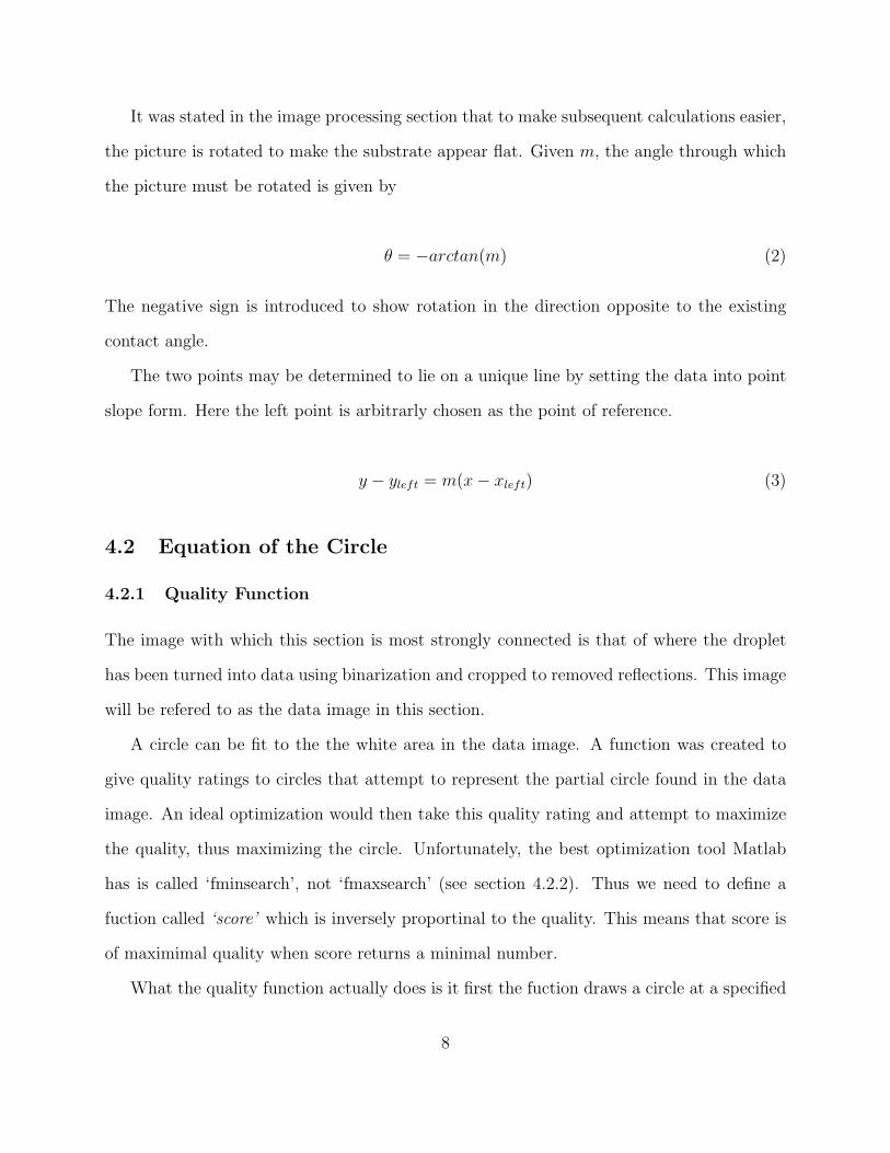
It was stated in the image processing section that to make subsequent calculations easier,

the picture is rotated to make the substrate appear flat. Given m, the angle through which

the picture must be rotated is given by

θ = −arctan(m) (2)

The negative sign is introduced to show rotation in the direction opposite to the existing

contact angle.

The two points may be determined to lie on a unique line by setting the data into point

slope form. Here the left point is arbitrarly chosen as the point of reference.

y − yleft = m(x− xleft) (3)

4.2 Equation of the Circle

4.2.1 Quality Function

The image with which this section is most strongly connected is that of where the droplet

has been turned into data using binarization and cropped to removed reflections. This image

will be refered to as the data image in this section.

A circle can be fit to the the white area in the data image. A function was created to

give quality ratings to circles that attempt to represent the partial circle found in the data

image. An ideal optimization would then take this quality rating and attempt to maximize

the quality, thus maximizing the circle. Unfortunately, the best optimization tool Matlab

has is called ‘fminsearch’, not ‘fmaxsearch’ (see section 4.2.2). Thus we need to define a

fuction called ‘score’ which is inversely proportinal to the quality. This means that score is

of maximimal quality when score returns a minimal number.

What the quality function actually does is it first the fuction draws a circle at a specified

8

starting location. The fuction then examines two categories. The first category is the overlap

between the drawn circle and the white area in the data image, this is labeled white’. The

second category is the overlap between the drawn circle and the black area, this is labeled

black’. The function then gives a merit based quality score displayed in Equation 4

score =1

|white− black|(4)

4.2.2 fminsearch

The purpose of the quality function is to be minimal when the drawn circle maximally

overlaps the white cirlce, and minimally overlaps any black area. Next the quality function

is given to the function ‘fminsearch(fun,x0)’. fminsearch(fun,x0) starts at the point x0 and

finds a local minimum x of the function described in fun. x0 can be a scalar, vector, or

matrix. fun is the name of a function. In this case x0 is a vector that details the radius and

center of a circle to be drawn. The local minimum x then uniquely specifies the optimal

circle to describe the white area; its center (xcenter = x0, ycenter = y0) and radius r0 are

logged.

4.3 Contact Points

The next objective is to find the location of the three-phase contact line. This is acheived by

finding the where the contact points. On the mathematical level this is equivalent to finding

where the circle and line intersect.

In general the equations a line and circle are

y − yleft = m(x− xleft) (5)

(x− x0)2 + (y − y0)

2 = r02 (6)

9

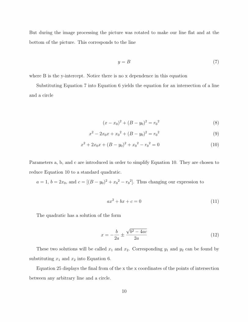
But during the image processing the picture was rotated to make our line flat and at the

bottom of the picture. This corresponds to the line

y = B (7)

where B is the y-intercept. Notice there is no x dependence in this equation

Substituting Equation 7 into Equation 6 yields the equation for an intersection of a line

and a circle

(x− x0)2 + (B − y0)

2 = r02 (8)

x2 − 2x0x + x02 + (B − y0)

2 = r02 (9)

x2 + 2x0x + (B − y0)2 + x0

2 − r02 = 0 (10)

Parameters a, b, and c are introduced in order to simplify Equation 10. They are chosen to

reduce Equation 10 to a standard quadratic.

a = 1, b = 2x0, and c = [(B − y0)2 + x0

2 − r02]. Thus changing our expression to

ax2 + bx + c = 0 (11)

The quadratic has a solution of the form

x = − b

2a±√

b2 − 4ac

2a(12)

These two solutions will be called x1 and x2. Corresponding y1 and y2 can be found by

substituting x1 and x2 into Equation 6.

Equation 25 displays the final from of the x the x coordinates of the points of intersection

between any arbitrary line and a circle.

10

x = −2x0

2±

√(2x0)

2 − 4(1) [(B − y0)2 + x02 − r0

2]

2(13)

x = −x0 ±√

x20

2− [(B − y0)2 + x0

2 − r02] (14)

The y-coordinate of the intersection is given as y = B by Equation 7.

4.4 Contact Angle

With the location of the contact points determined, one can combine all collected data and

thus determine the contact angle of a droplet on a substrate.

The slope of the tangent to a curve at any given point is given by the derivative at that

point. Using implicit differentiation, we know the slope of the line tangent to a circle is given

by

d

dx

((x− x0)

2 + (y − y0)2)

=d

dx(r0

2) (15)

2(x− x0) + 2(y − y0)y′ = 0 (16)

y′ = −(

x− x0

y − y0

)(17)

Where y′ = dy/dx is the equation of a line tangent to a circle at the contact points (note:

not the line). Plugging in for (x1, y1) and (x2, y2) gives the slope of the line tangent to the

circle at the corresponding points.

The angles between the slope of the line tangent to the circle y′ and the slope of the

substrate surface m = 0 are the contact angles. For ease of calculation, both slopes are

converted into vector format, diplayed in Figure 3. The vectors represent the changes cor-

responding to taking a step of unit length in the ±x̂ direction from contact points (x1, y1)

11

and (x2, y2). At the left contact point, the step is taken in the +x̂ direction and at the

right contact point the step is taken in the −x̂ direction. Thus the vectors that describe the

tangents to the droplet (at the contact points) and the substrate given by

~v1 = [y′(x1, y1) 1] (18)

~v2 = [0 1] (19)

~v3 = [y′(x2, y2) 1] (20)

~v4 = −[0 1] (21)

The angle between vectors ~v1 and ~v2 gives the left contact angle, and the angle between

vectors ~v3 and ~v4 gives the right contact angle. The expression for the angle between two

vectors is

θ = cos−1

(~u1 · ~u2

|| ~u1|| || ~u2||

)(22)

Using the four supplied vectors it is possible to determine the two contact angles.

12

5 Error Analysis

There are errors associated with every measurement and because this program measures

a contact angle. According to statistical theory, the error associated with any group of

measurements taken on a contact angle is given by the standard deviation. Because the

mean value for each contact angle was not known beforehand, the standard deviation is

given by

σ =

√Σx2

N − 1(23)

Where x = θ − θ0, the difference between any contact angle and the mean contact

angle associated with that calculation. All physically calculated contact angles had errors

of δθ = 0.5◦ because the smallest incrementation on the protractor used to calculate the

contact angles was 50.5◦.

To test the extent of these errors, the program was tested against three known angles.

The first contact angle examined was that of a in 45.0 ± 0.5◦ right triangle. The triangle

was aligned so that the 90◦ angle was pointed straight up. The program found the right

triangle to have a contact angle of 43.3± 2.6 ◦. A larger uncertainty with this contact angle

is expected because of the systematic problem of the program fitting only circles and not

triangles. The second angle examined was a computer generated shaded circle piece. This

circle piece has a contact angle of 45.0±0.5◦. The circle was made large enough so that there

is negligible error associated with the contact angle. The program was used on the shaded

circle, marking the corners of the circle as contact points. The program returned a contact

angle of θ = 90.2 ± 0.5◦. Lastly, the program was used to analyze the picture of a droplet.

Using a computer printout, the droplet was found to have contact angle of θ = 67.3± 0.5◦,

while the program displayed contact angles of θ = 68.1±1.3◦. Systematic uncertainties arise

with identifying the exact location of the three-phase contact line in the droplet image.

13

6 Program Code for Determining Contact Angles

The latter sections detailed the general method of how a program determines the contact

angle of a droplet on a substrate at the three-phase contact line. This section describes

in-depth the actual program and what its doing, every step of the way.

Before describing program implementation, a few notes on writing structure are in order.

The code is broken into separate tasks. Each task acts as a piece of information separate

from the rest of the code. All major image processing changes are marked with new figures,

e.g. figure(1), and are terminated with some function that calls for the image to be displayed,

e.g. imshow, imagesc. The purpose of displaying an image at the end of each section was to

aid the user in following the image processing changes made to the pictures by the program.

6.1 Special Functions

Throughout the course of the program, there are two special special functions that are

repeatedly called by the program. These functions are special because they were written

by the program designer. The functions are essential in the process of finding the contact

angle at the three-phase contact line. Although the functions have task numbers thirteen

and fourteen, they do not occur in that order. The functions are called when needed, and

after completing a task, each function returns to the line of the program from which it left.

6.1.1 Create an Image with Fitted Circle Points

One of the two special functions is named ‘circle’. The function draws a circle at a specified

location on a background of specified size. ‘circle’ requires inputs that define the radius,

location of the center of a circle, and an image.

First the function specifies the bounds of the area on which drawing is to occur. This is

defined to be from −radius to +radius. The domain is then further restricted to be circular.

14

Next a matrix of zeroes defines the background based on the size of the input image. Finally

the bounded circular domain is placed in the location entitled center within the matrix. All

the points within this circle are turned white while the rest of the circle remains black. The

function circle outputs a matrix that has a circle at a prespecified location with a prespecified

radius of a prespecified image size.

6.1.2 Determine Circle Quality, as a Fitting Figure of Merit

Task fourteen defines the special function ‘fit fun’. This function compares a picture with

a drawing and determines a quality value based on similarities between the two. ‘fit fun’ is

superficially described in section 4.2. The quantity ‘val’ goes down as the quality of the test

circle increases. ‘fit fun’ requires inputs that define the radius, location of the center of a

circle, and an image.

The first thing ‘fit fun’ does is create a mock circle, by calling the other special function

‘circle’. ‘circle’ returns a matrix of a circle. Next ‘fit fun’ defines the output parameter ‘val’.

‘val’ examines the overlap between the white area in the data image (BW4) and the image

of the drawn circle (crcl), as well as the overlap of the white area in crcl and the black area

in BW4. The value of a drawn circle is finally determined by

val =

∣∣∣∣∣ 1

||BW ∪ crcl|| − ||crcl ∪ B̃W ||

∣∣∣∣∣ (24)

Where ||BW ∪ crcl|| and ||crcl ∪ B̃W || are the sizes of the overlaps.

6.2 Main Program Code

The Main Program runs through a list of tasks, with each task building on the information

from the previous tasks. The program is, in this way, comprised of twelve individual tasks

that are necessary for calculating the contact angle of a droplet on a substrate.

15

6.2.1 Initializing the Program

The first task is to initialize the program. This involves calling the image that had been

prepared for analysis, and closing all windows that may be open. A grayscale version of the

original image is displayed on the screen.

6.2.2 Convert to Gray

Next a new window is opened, and in it is displayed a grayscale version of the image created

in when initializing the program. Additionally, the image is changed to from a regular ‘img’

type, to the type ‘double’. This is in preparation for later on: only images of type ‘double’

may be converted to binary images.

6.2.3 Remove Background Noise

To remove the backround noise it is necessary to have the computer recognize the droplet

and the background as two distinct objects. The first portion of this task was to create

as uniform a background as possible, so as to highlight the droplet from the rest of the

picture. The idea here is to create an image that resembles the non-uniform background.

By subtracting this noise from the standard image, a the background is made more uniform.

This normalized background image was created by using the imformation at the corners. In

order to create an accurate background image, the four pixels nearest to each corner were

used. The mean intesity of the four pixels closest to each corner defines the intensity value

at that corner to be used in the image named ‘background’. The values of grayscale intensity

near the corners of the image sampled, and these values are given in Matlab by the lines

im(1:2,1:2), im(1:2,end-[0:1], im(end-[0:1],1:2), im(end-[0:1],end-[0:1])

The meshgrid takes the mean values of each corner and interpolates values intermediary

values. After determining how many values should be interpolated in each direction, the

meshgrid values are saved in the image named ‘background’. In the program, the size of the

16

meshgrid as based on the size of the original picture. The size of the original picture was

stored in the values a.inp, b.inp, a.out, and b.out. The background picture was also defined

in size by a.inp, b.inp, a.out and b.out, making the original picture and the background

picture the same size. Next, the interpolated background data was subtracted from the

original image to create a ‘corrected’ image. The corrected image is the final result of the

task one with a more uniform background. The image is then displayed on a grayscale.

Without this function it would be much harder to clearly define what is an edge, and what

is not. The meshgrid interpolated smooth transitions between the intensity values at each

corner. The interpolated image was then named ‘background’.

6.2.4 Black and White Image

This task transforms the corrected image, that highlighted the droplet, into binary data.

This data is later used to extract the contact angle at the three-phase contact line. In this

step the water droplet is not only highlighted; for the first time it is set apart from the rest of

the data. From a programming perspective, section ‘figure(3)’ changed the corrected image

from figure(2) into a black and white image, ’BW’. This was done using im2bw. The 0.02

appearing in the im2bw function was an adjustable parameter. This parameter could be set

to different values in order to make to adjust the intensity above which an individual pixel

turns white.

6.2.5 Identify Droplet

To identify the droplet in the picture, the program identified regions of the picture that could

be droplets. These were regions where there were a lot of white points clustered together.

An assumption was made that the largest white region defined the droplet. All regions that

weren’t a member of the largest region were then identified as noise, and were therefore

removed. Thus the data is refined to be only from the region believed to be the droplet.

17

All the data in figure(3) was searched through for the region that could be the droplet.

Within this data ’L’ labeled all the regions that were contiguous. Contiguous regions were

defined as being one of the four closest squares to each other piece of data, e.g. directly to

the left, right, above or below another piece of the remaining data. The labeling is done

using the function bwlabeln. the size ’S’ of each labeled region was then found with the

regionprops function. Finally the largest region is then determined by using a combination

of the ismember, find, and max functions. The ismember gives out an input of true or false.

The code was then configured to delete all data that’s not part of the largest section, and

thus, not part of the droplet. The resultant image is then displayed as figure(4).

6.2.6 Fill in Droplet

The previous task filtered external noise, but section six filters noise within the droplet. The

internal noise results from parts of the droplet that didn’t stand out very much and were

subsequently assumed to be non-droplet area. The droplet image data was then restored

using the imfill command. The image figure(5) displays the doctored droplet.

6.2.7 Identify Substrate

In this task the user is called upon to input data during the program. The user interaction

plays an integral role in droplet image processing. As can be seen in IMAGE Y a reflec-

tion of the droplet on the substrate cannot be distinguished from the image of the original

droplet. This reflection occurs along the substrate surface. Identifying this line is crucial for

determining the contact angle. Contact angles are measured with respect to this substrate

surface. Furthermore substrate surface is not easy to determine by computer logic. The

program is based on a human’s ability to input the left and right edges of the water droplet.

The coordinates of the information received were put into two vectors: x coordinates and

y coordinates. This was done using the impixel function. The impixel function also displays

18

the intensity of the pixel selected, but this information is not used.

6.2.8 Prepare for Circular Fitting

The first action undertaken to prepare for the circular fitting was to develop an equation

representing the substrate surface. The y-intercept and the angle that the substrate surface

makes with respect to the edge of the picture are stored. After obtaining this information it

is possible to remove the reflection image from the rest of the image, leaving only the actual

droplet. First the image is truncated to the level of the substrate surface. Next the image

was rotated to make the substrate surface flush with the bottom of the picture. The image,

figure(6), is then displayed. From this state it is very easy to determine the contact angle.

6.2.9 Initialize Circular Fit

Task nine initializes the circular fitting process, discussed in the section entitled ‘Equation

of the Circle’. The program looks at two special functions ‘fit fun’ and ‘circle’, that have

parameters corresponding to the location of the center of a circle, as well as BW4, the

matrix representation of figure(6). From these parameters the special function ‘circle’ draws

an initial circle, centered at (200,300) with initial radius 250. The special function ‘circle’

will be discussed in depth in task 13. ‘fit fun’ then examines the overlap between the circle

drawn with ‘circle’, and the white region from BW4. ‘fit fun’ determines a quality value

based on how much the drawn circle overlaps the white region, and how little the drawn

circle overlaps the black region. A circle that corresponds to the data well has a lower quality

value.

6.2.10 Fit Best Circle

This task finds finds the best-fit circle that matches the black and white droplet image. The

circle is fit by finding the lowest possible quality value, and recording the corresponding

19

center and location of the circle. The lowest possible quality value is determined using the

Matlab function fminsearch. In this case, the variable ‘cntr radius’ is a vector comprised

three components. These components correspond to the center of the circle (both x and

y) and the radius of the circle. As will be explained in further detail later, fit fun gives a

quality value that will be minimal when the drawn circle best resembles the white region in

the image BW4.

6.2.11 Display Confirmation Picture

After determining the equation for the best-fit cirlce, this section displays an image to confirm

that the fitting worked. The optimized circle is made into an image and then overlayed

with the original picture. The two images can be simultaneously viewed using the function

imagesc. In order to distinguish the original image from the fitted image, the values of the

fitted image is multiplied by ten, making the fitted image appear red in figure(7).

6.2.12 Calculate Contact Angles

Task tweleve does the actual contact angle calculation. The contact angle is calculated by

finding the angle between the vectors tangent to the circle and the substrate surface (see

Figure 3). The technical details for understanding task twelve require a bit of geometry, and

not just programming. Please refer to the section entitled Mathematical Manipulation for

further reference. To calculate the contact angles it is necessary to know vectors ~v1 - ~v4. The

tangent to the circle at the contact points must be calculated in order to know ~v1 and ~v3.

The contact points are given as the points where the circle intersects with the line. From

Equation 25

x = −x0 ±√

x20

2− [(B − y0)2 + x0

2 − r02] (25)

20

the x-coordinates are known. Here x0 and y0 represent location of the center of the circle,

and r0 represents the radius of the circle. Notice it is not necessary to find the y-coordinate,

because after making the substrate surface flush with the bottom of the picture, the equation

for the y-intercept is given by y = 1. In the program these coordinates are stored as the

vector ‘contact pt’. The slope of line tangent to the circle is given by Equation 26.

y′ = −contact pt(1)− x0

contact pt(2)− y0

(26)

Where x0 and y0 again represent location of the center of the circle.

With y′ thus determined at the contact points it is possible to construct the vectors ~v1

and ~v3. The contact angle is calculated in radians. Multiplying by 180π

converts the contact

angle to degrees.

The final step is to make sure the angles correspond to the coordinate in the proper

quadrant. Inverse trigonometric functions can detail information about the location of a

point in only two quadrants. To correct for the discrepancy, it is necessary to use the mod

function.

The corrected contact angle is finally displayed and the program is complete.

21

7 Using the Program

7.1 Preparation

Using the program requires the user know the name of the droplet image they want to use.

The user must make sure the file to be used, and the file contact angle.m are in Matlab’s

active directories. If an optimization fails, to produce physical results, it is sometimes it is

necessary to make changes pertaining to the initializing circle in tasks nine and ten. The

original center and radius are set at [200, 300], 250, which is good for contact angles in the

range of 40◦ to 110◦, but these values do not produce good results for water on silicon, which

has a contact angle of ≈ 30◦. For small angles, initialization parameters are recommended

as [200, 550], 300.

7.2 Program

The program begins with the user typing in the command ‘contact angle(*)’. The * can

represent any standard rgb image. For ease of discussion assume the image is named droplet.

The program then displays five figures. The first figure displays a grayscale picture of

droplet.

22

8 Program Code

%*******************************************************************************

%***** Determining the Contact Angle of Water on a Substrate *****

%*******************************************************************************

%*******************************************************************************

% 1. Initializing the Program *

%*******************************************************************************

function saknduck % Function name

file = ’/home/duck/Duck1_137a/snapshot-20070827-152218.png’ % Image Location

close all; % Close all windows

%*******************************************************************************

% 2. Convert to Gray *

%*******************************************************************************

figure(1); % Create a new figure

im = im2double(rgb2gray(imread(file ))); % Convert image to gray

imshow(im ); % Display image

%*******************************************************************************

% 3. Remove Background Noise *

%*******************************************************************************

figure(2); clf; % New Figure

% Meshgrid sets the domain domain for variables to be used in calculations.

% Domain is determined by picture size

[a.inp,b.inp] = meshgrid( [ 1 size( im, 2)], [1 size(im,1)] )

[a.out,b.out] = meshgrid( [ 1:size( im, 2)], [1:size(im,1)] )

% Background noise simulation based on information near corners

background = interp2(a.inp, b.inp, [mean(mean(im(1:2,1:2))), ...

mean(mean(im(1:2,end-[0:1]))); mean(mean(im(end-[0:1],1:2))), ...

mean(mean(im(end-[0:1],end-[0:1]))) ], a.out, b.out );

corrected = im - background; % Subtracts off background changes

imagesc( corrected, [min(corrected(:)), max( corrected(:))] );

% Display intensity based image

colormap( ’gray’ ); % Display grayscale of intensity image

%*******************************************************************************

% 4. Black and White Image *

%*******************************************************************************

figure(3); clf; % New Figure

BW = im2bw(corrected, 0.02); % Make Image Black and White

imshow( BW ); % Display Image

%*******************************************************************************

% 5. Identify Droplet *

%*******************************************************************************

figure(4); clf; % New Figure

L = bwlabeln(1-BW, 4); % Label White Spots

S = regionprops(L, ’Area’); % Measure Area of Spots

BW2 = ismember(L, find([S.Area] ==max( [S.Area]) )); % Find Largest Spot

BW2(1,:) = 1; % Turn First Row White

imshow( BW2 ) % Display Image

23

%*******************************************************************************

% 6. Fill in Droplet *

%*******************************************************************************

figure(5); clf; % New Figure

BW3 = imfill( BW2, ’holes’ ); % Fill In Holes in Image

imshow( BW3 ); % Display Image

%*******************************************************************************

% 7. Identify Substrate *

%*******************************************************************************

% Human Clicks on Contact Points of Water on Substrate

[x_coordinates y_coordinates Pixel_vals] = impixel;

%*******************************************************************************

% 8. Prepare for Circular Fitting *

%*******************************************************************************

figure(6); clf; % New Figure

rot_line = polyfit(x_coordinates ,y_coordinates ,1 ); % Replicate Substrate

rot_point = round( polyval( rot_line, 1 )); % Truncation Point

rot_angle = atan( rot_line(1) ); % Correction Angle

BW4 = BW3( rot_point:end,: ); % Truncation

BW4 = imrotate( BW4, -rot_angle*180/pi ); % Correction

BW4 = BW4( -y_coordinates(2) + rot_point:end,: ); % Truncation Correction

imshow( BW4 ); % Display Image

%*******************************************************************************

% 9. Initialize Circular Fit *

%*******************************************************************************

% Finds an initial quality value, see (14) fit_fun for details

fit_fun( [200 300], 250, BW4 )

%*******************************************************************************

% 10. Fit Best Circle *

%*******************************************************************************

% Optimizes quality value, see (14) fit_fun for details

[val, status, message] = fminsearch( @(cntr_radius) ...

fit_fun( cntr_radius(1:2), cntr_radius(3), BW4 ), ...

[200, 200, 100], optimset( ’display’, ’iter’ ) )

%*******************************************************************************

% 11. Display Confirmation Picture *

%*******************************************************************************

figure(7);clf; % New Figure

crcl = circle( val(1:2), val(3), size(BW4) ); % Optimized Generated Circle

imagesc( 10*crcl+BW4 ); % Picture/Optimization Overlay

axis image; % Show axes

24

%*******************************************************************************

% 12. Calculate Contact Angles *

%*******************************************************************************

% Math manipulation to calculate contact points based on radius and

% location of the center of the circle

contact_pt = [ (sqrt( val(3)^2 - ( 1-val(1) )^2 ) + val(2)), ...

-(sqrt( val(3)^2 - ( 1-val(1) )^2 ) + val(2)) ];

% Determine tangent lines of contact points

tangent_slope = -( contact_pt-val(2) )/( 1-val(1) );

contact_angle = atan(tangent_slope); % Contact Angle

contact_angle = contact_angle*180/pi; % Radians to Degrees

corrected_angle = [ mod( 180-contact_angle(1), 180 ), ...

mod( 180+contact_angle(2), 180 )] % Correction for proper domain

return

%*******************************************************************************

% Finish Main Program

%*******************************************************************************

%***** Special Functions Called by Tasks 9 and 10 *****

%*******************************************************************************

%*******************************************************************************

% 13. Create an Image with Fitted Circle Points *

%*******************************************************************************

function subim = circle( center, radius, sz ); % Function called circle

[a,b] = ndgrid( -radius:radius ); % Restrict domain to radius

tmp = a.^2+b.^2<= radius^2; % Make Domain Circular

subim = zeros( sz ); % Matrix of Zeros

subim(round(min(end, max(1,center(1)+[-radius:radius]) )), ...

round(min(end, max(1,center(2)+[-radius:radius]) )) ) = tmp; % Draw Circle

return;

%*******************************************************************************

% 14. Determine Circle Quality, as a Fitting Figure of Merit *

%*******************************************************************************

function [val] = fit_fun( center, radius, BW ) % Function called fit_fun

crcl = circle( center, radius, size( BW ) ); % Create Circle

val = 1/abs(sum(sum(BW&crcl) )-sum(sum(crcl&~BW))); % Value Drawing’s Accuracy

return;

25

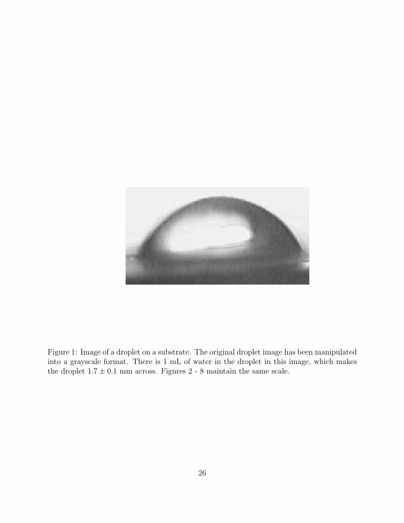
Figure 1: Image of a droplet on a substrate. The original droplet image has been manipulatedinto a grayscale format. There is 1 mL of water in the droplet in this image, which makesthe droplet 1.7± 0.1 mm across. Figures 2 - 8 maintain the same scale.

26

Figure 2: Droplet highlighted from its background. The background appears, much smootherthan in Figure 1.

27

Figure 3: The grayscale image converted to black and white only. In this image the droplet isblack and non-droplet areas are white. The black line at the top of the picture is an artifactfrom image processing.

28

Figure 4: This black and white image has eliminated all background noise, to further dis-tinguish the droplet from the background. Furthermore, the droplet has been converted towhite and the non-droplet areas are black.

29

Figure 5: The program mistakes some of the droplet as background. This error is correctedby filling in all black regions contained within a white region.

Figure 6: A user clicks the three-phase contact line at the left and right sides of the dropletin Figure 1. Shown at the left side of the picture is a mark from the user in placing a threephase contact-line placement indicator. On the right the user is about to place another suchindicator. These indicators are placed where the droplet, the liquid, and the air all meet.

30

Figure 7: The droplet reflection has been removed, and the droplet is set as flush againstthe bottom of the screen. On the right side of the screen there is a thin white line left overfrom image processing.

Figure 8: After optimization the droplet is overlayed with a circle of best fit. The backgroundregion is set as deep blue, the region where theres only droplet is set as light blue, the regionwhere theres only circle is set as light red, the region where droplet and circle overlap is darkred.

31

Figure 9: An picture showing key features of a droplet. These features are all noted in theprogram.

32