Determining Nanocapillary Geometry from Electrochemical ......Determining Nanocapillary Geometry...

Determining Nanocapillary Geometry fromElectrochemical Impedance Spectroscopy Using aVariable Topology Network Circuit Model

Michael J. Vitarelli, Jr.,† Shaurya Prakash,*,‡ and David S. Talaga*,§

Department of Chemistry and Chemical Biology, Rutgers University, 610 Taylor Road, Piscataway,New Jersey 08854, United States, Department of Mechanical Engineering, The Ohio State University, 201 West 19thAvenue, Columbus, Ohio 43210, United States, and Department of Chemistry and Biochemistry, Montclair StateUniversity, 1 Normal Road, Montclair, New Jersey 07043, United States

Solid-state nanopores and nanocapillaries find increasinguse in a variety of applications including DNA sequencing,synthetic nanopores, next-generation membranes for wa-ter purification, and other nanofluidic structures. Thispaper develops the use of electrochemical impedancespectroscopy to determine the geometry of nanocapillar-ies. A network equivalent circuit element is derived toinclude the effects of the capacitive double layer insidethe nanocapillaries as well as the influence of varyingnanocapillary radius. This variable topology function issimilar to the finite Warburg impedance in certain limits.Analytical expressions for several different nanocapillaryshapes are derived. The functions are evaluated to deter-mine how the impedance signals will change with differentnanocapillary aspect ratios and different degrees of con-striction or inflation at the capillary center. Next, thecomplex impedance spectrum of a nanocapillary arraymembrane is measured at varying concentrations ofelectrolyte to separate the effects of nanocapillary doublelayer capacitance from those of nanocapillary geometry.The variable topology equivalent circuit element model ofthe nanocapillary is used in an equivalent circuit modelthat included contributions from the membrane and themeasurement apparatus. The resulting values are con-sistent with the manufacturer’s specified tolerances of thenanocapillary geometry. It is demonstrated that electro-chemical impedance spectroscopy can be used as a toolfor in situ determination of the geometry of nanocapillaries.

Individual solid-state nanopores or nanocapillary array mem-branes (NCAMs) are routinely fabricated1,2 and have been usedextensively in recent years to develop synthetic systems for ion-channel studies,3-7 single molecule sensing,8,9 DNA sequencing,1,10

nanofabrication templates,11,12 and fundamental studies of ionicflow at the nanoscale.13,14 Track-etched arrays of nanocapillariesin polymeric membranes15,16 are commercially available and havebeen used for permselectivity,17 as molecular gates for nanoscaleflow control,18 and for identification of transport regimes as afunction of electrokinetic radius.14 These applications establishedthat solution-phase transport through the membrane is affectedby the geometry and surface properties of the nanocapillaries bothof which can change depending on solution conditions.19,20

Therefore, in situ methods for determining the geometry andsurface properties of nanocapillaries are vital for understandinganalyte transport and analyte-capillary interactions.

Ideally, in situ characterization of the nanocapillary geometrywould be by a nondestructive method that is based on thetransport physics relevant to the intended application. High-

* To whom correspondence should be addressed. E-mail: [email protected] (S.P.); [email protected] (D.S.T.).

† Rutgers University.‡ The Ohio State University.§ Montclair State University.

(1) Dekker, C. Nat. Nanotechnol. 2007, 2, 209–215.(2) Piruska, A.; Gong, M.; Sweedler, J. V.; Bohn, P. W. Chem. Soc. Rev. 2010,

39, 1060–1072.(3) Tian, Y.; Hou, X.; Wen, L.; Guo, W.; Song, Y.; Sun, H.; Wang, Y.; Jiang, L.;

Zhu, D. Chem. Commun. 2010, 46, 1682–1682.

(4) Siwy, Z.; Howorka, S. Chem. Soc. Rev. 2010, 39, 1115–1132.(5) Holt, J. K.; Park, H. G.; Wang, Y.; Stadermann, M.; Artyukhin, A. B.;

Grigoropoulos, C. P.; Noy, A.; Bakajin, O. Science 2006, 312, 1034–1037.(6) Siwy, Z.; Heins, E.; Harrell, C.; Kohli, P.; Martin, C. J. Am. Chem. Soc. 2004,

126, 10850–10851.(7) Steinle, E.; Mitchell, D.; Wirtz, M.; Lee, S.; Young, V. Y.; Martin, C. Anal.

Chem. 2002, 74, 2416–2422.(8) Howorka, S.; Siwy, Z. Chem. Soc. Rev. 2009, 38, 2360–2384.(9) Chen, Z.; Jiang, Y.; Dunphy, D. R.; Adams, D. P.; Hodges, C.; Liu, N.; Zhang,

N.; Xomeritakis, G.; Jin, X.; Aluru, N. R.; Gaik, S. J.; Hillhouse, H. W.;Brinker, C. J. Nat. Mater. 2010, 9, 667–675.

(10) Branton, D.; Marziali, A.; Deamer, D. W.; Bayley, H.; Benner, S. A.; Butler,T.; Di Ventra, M.; Garaj, S.; Hibbs, A.; Huang, X.; Jovanovich, S. B.; Krstic,P. S.; Lindsay, S.; Ling, X. S.; Mastrangelo, C. H.; Meller, A.; Oliver, J. S.;Pershin, Y. V.; Ramsey, J. M.; Riehn, R.; Soni, G. V.; Tabard-Cossa, V.;Wanunu, M.; Wiggin, M.; Schloss, J. A. Nat. Biotechnol. 2008, 26, 1146–1153.

(11) Gultepe, E.; Nagesha, D.; Menon, L.; Busnaina, A.; Sridhar, S. Appl. Phys.Lett. 2007, 90, 163119/1–163119/3.

(12) Lu, Z.; Namboodiri, A.; Collinson, M. ACS Nano 2008, 2, 993–999.(13) Raghunathan, A. V.; Aluru, N. R. Phys. Rev. E: Stat., Nonlinear, Soft Matter

Phys. 2007, 76, 011202/1–011202/12.(14) Kemery, P. J.; Steehler, J. K.; Bohn, P. W. Langmuir 1998, 14, 2884–2889.(15) Lee, S. B.; Martin, C. R. J. Am. Chem. Soc. 2002, 124, 11850–11851.(16) Prakash, S.; Yeom, J.; Jin, N.; Adesida, I.; Shannon, M. A. Proc. Inst. Mech.

Eng., Part N 2007, 220, 45–52.(17) Nishizawa, M.; Menon, V. P.; Martin, C. R. Science 1995, 268, 700–702.(18) Tulock, J. J.; Shannon, M. A.; Bohn, P. W.; Sweedler, J. V. Anal. Chem.

2004, 76, 6419–6425.(19) Prakash, S.; Karacor, M. B.; Banerjee, S. Surf. Sci. Rep. 2009, 64, 233–

254.(20) Prakash, S.; Piruska, A.; Gatimu, E. N.; Bohn, P. W.; Sweedler, J. V.;

Shannon, M. A. IEEE Sens. J. 2008, 8, 441–450.

Anal. Chem. 2011, 83, 533–541

10.1021/ac102236k 2011 American Chemical Society 533Analytical Chemistry, Vol. 83, No. 2, January 15, 2011Published on Web 12/28/2010

resolution electron microscopy can image the geometry;21-23

however, it requires extensive sample preparation, usually render-ing the sample unusable for its application. Current-voltagemeasurements have been reported that show evidence of surface-charge related rectification.24-26 These dc-based methods do notgive direct information about the geometry of the nanocapillaries.By contrast, electrochemical impedance spectroscopy, or EIS,27-29

measures the impedance as a function of frequency of applied acpotential.

Since the EIS signal is a measure of the electrokinetic transportof ionic solution through the nanocapillaries, it is sensitive to theirgeometry and surface electrical properties.30,31 The measuredsignal is governed by electrokinetic transport equations that arelaborious to implement for characterization of arbitrary nanofluidicsystems32 and therefore are not practical for routine laboratoryuse. Equivalent circuit modeling is a standard approach to fittingEIS data.33,34 Nanocapillary physical parameters such as geometryand double layer differential capacitance must be interpreted fromthe fit parameters. A disadvantage of this approach is multipleequivalent circuits can be fit to the same data. This problemincreases as the number of equivalent circuit elements in themodel increases. Therefore, the number of elements required inan equivalent circuit model should be minimized while stillcapturing the relevant physics.

EIS has been previously applied to NCAMs. In these casesR|C circuits have been used to extract resistive and capacitiveproperties, the effect of a dc bias on these properties, and theeffects of foulants on the NCAMs.16,35-38 However, R|C equivalentcircuit models have not been used to quantify the geometry ofthe nanocapillaries. Moreover, specific equivalent circuit modelshave not been developed that explicitly include details of thenanocapillary geometry and surface properties.

The purpose of this paper is to develop a new equivalent circuitelement that, when coupled with the standard approach ofequivalent circuit modeling, can obtain the nanocapillaries geom-etry and double layer differential capacitance. Previously, a relatedequivalent circuit model was used to derive expressions todetermine the average shape of closed capacitive pores.39 Thenew equivalent circuit element predicts that the shape of EIS datawill depend on the aspect ratio of the capillaries and on anyconstrictions present in the capillaries. These geometric effectswould be indeterminable from simple current-voltage curves thatgive the zero-frequency dc limit of the impedance. Formulas forseveral specific parametrized nanocapillary geometries are derivedand compared with experimental data. The new impedanceelement was used to model EIS measurements on an NCAM ofnominal pore radius of 5 nm. Measurements at different solutionconductivities were used to separate the effects of geometry anddouble layer differential capacitance in the EIS data. The newimpedance element was able to invert EIS data to nanocapillarygeometry when used in a simple equivalent circuit model thatalso included the response of the membrane and experimentalapparatus. The limitations and assumptions of the model arecritically discussed in terms of its ability to reproduce the dataand nanocapillary parameters.

METHODSTwo glass chambers sandwich two cylindrical pieces of

poly(dimethylsiloxane) (PDMS), with a NCAM (GE KN1CP02500)in between. The manufacturer specified that the NCAM hasnanocapillary density of 6 × 108 capillaries/cm2 ± 15%, a thicknessof 6 µm ± 10%, prepared by track etching for a nominal poreradius of 5 nm +0% -20%. The glass chambers contain 5 mLof the test electrolyte solution in 18 MΩ Millipore water witha known concentration of electrolytes as discussed below. Ag/AgCl reference electrodes (MF-2052, Bioanalytical Systems,Inc.) and gold wire counter electrodes were used. The PDMScylinders have a 0.60 cm diameter hole for an exposed NCAMsurface area Amem of 0.283 cm2. The PDMS pieces are bondedfollowing exposure to 30 W oxygen plasma.40-42 All experimentswere performed in a copper mesh Faraday cage to minimizeelectrical noise. The Au counter electrodes were RCA-1 cleanedbefore each experiment.43 A schematic of the experimental setupis located in the Supporting Information.

NCAMs require equilibration prior to use.7 Prior to use, themembranes were soaked in 18 MΩ Millipore water for 48 h. Priorto each experiment, they were soaked at the experimental solutionconditions for 4 h. It is critical to maintain a constant pH so as topreserve the membrane surface charge density,19 which deter-mines the double layer capacitance.27 A 10 mM sodium phosphatebuffer was used to fix the pH at 7.0 ± 0.1 at each of the fiveconcentrations of NaCl: 100, 50, 20, 10, 0 mM. Bulk conductivitiesof these solutions were interpolated from published values.44

(21) Wu, M.-Y.; Smeets, R. M. M.; Zandbergen, M.; Ziese, U.; Krapf, D.; Batson,P. E.; Dekker, N. H.; Dekker, C.; Zandbergen, H. W. Nano Lett. 2009, 9,479–484.

(22) Storm, A. J.; Chen, J. H.; Ling, X. S.; Zandbergen, H. W.; Dekker, C. Nat.Mater. 2003, 2, 537–540.

(23) Fologea, D.; Uplinger, J.; Thomas, B.; McNabb, D. S.; Li, J. Nano Lett. 2005,5, 1734–1737.

(24) Karnik, R.; Fan, R.; Yue, M.; Li, D.; Yang, P.; Majumdar, A. Nano Lett. 2005,5, 943–948.

(25) Schoch, R.; Han, J.; Renaud, P. Rev. Mod. Phys. 2008, 80, 839–883.(26) Stein, D.; Kruithof, M.; Dekker, C. Phys. Rev. Lett. 2004, 93, 035901/1–

035901/4.(27) Bard, A. J.; Faulkner, L. R. Electrochemical Methods: Fundamentals and

Applications; John Wiley & Sons: Hoboken, New Jersey, 1980.(28) Barsoukov, E.; MacDonald, R. Impedance Spectroscopy: Theory, Experiment,

and Applications, 2nd ed.; John Wiley & Sons: Hoboken, New Jersey, 2005.(29) Macdonald, J. R. Impedance Spectroscopy: Emphasizing Solid Materials and

Systems; John Wiley and Sons: Hoboken, New Jersey, 1987.(30) Ervin, E. N.; White, H. S.; Baker, L. A.; Martin, C. R. Anal. Chem. 2006,

78, 6535–6541.(31) Ervin, E. N.; White, H. S.; Baker, L. A. Anal. Chem. 2005, 77, 5564–5569.(32) Chilcott, T. C.; Chan, M.; Gaedt, L.; Nantawisarakul, T.; Fane, A. G.; Coster,

H. G. L. J. Membr. Sci. 2002, 195, 153–167.(33) Macdonald, D. D. Electrochim. Acta 2006, 51, 1376–1388.(34) Macdonald, J. R. Electrochim. Acta 1990, 35, 1483–92.(35) Kavanagh, J. M.; Hussain, S.; Chilcott, T. C.; Coster, H. G. L. Desalination

2009, 236, 187–193.(36) Coster, H.; Chilcott, T. Surface Chemistry and Electrochemistry of Membranes;

Marcel Dekker, Inc.: New York, 1999.(37) Coster, H. G. L.; Kim, K. J.; Dahlan, K.; Smith, J. R.; Fell, C. J. D. J. Membr.

Sci. 1992, 66, 19–26.(38) Gaedt, L.; Chilcott, T. C.; Chan, M.; Nantawisarakul, T.; Fane, A. G.; Coster,

H. G. L. J. Membr. Sci. 2002, 195, 169–180.

(39) Kaiser, H.; Beccu, K. D.; Gutjahr, M. A. Electrochim. Acta 1976, 21, 539.(40) Duffy, D. C.; McDonald, J. C.; Schueller, O. J. A.; Whitesides, G. M. Anal.

Chem. 1998, 70, 4974–4984.(41) McDonald, J. C.; Whitesides, G. M. Acc. Chem. Res. 2002, 35, 491–499.(42) Hillborg, H.; Ankner, J. F.; Gedde, U. W.; Smith, G. D.; Yasuda, H. K.;

Wikstrom, K. Polymer 2000, 41, 6851–6863.(43) Kern, W.; Puotinen, D. A. RCA Rev. 1970, 31, 187–206.(44) Weast, C. R., Ed. CRC Handbook of Chemistry and Physics; CRC Press, Inc.:

Boca Raton, FL, 1989-1990.

534 Analytical Chemistry, Vol. 83, No. 2, January 15, 2011

These values matched well with conductivity measurements madebased on determining the cell constant and instrument without amembrane present but showed some deviations at high ionicstrengths. (See the Supporting Information.)

A Gamry Instruments Reference 600 potentiostat was used toapply the potentials and measure the impedance in the system ina standard four-electrode permeation cell mode. In this work, theapplied potentials were kept low (10 mV ac amplitude and no dcbias) to minimize any Faradaic reactions. Furthermore, thereference electrodes are connected to a high impedance input anddraw negligible current. A total of 67 frequencies were measuredranging from 0.1 Hz to 1 MHz. Measurements were made foreach solution condition with and without the membrane presentto determine the cell constant and instrument response. Eachexperiment was repeated four times with a maximum variabilityof 0.8%, in the magnitude of impedance, and the data reported isthe average of these measurements.

Each EIS measurement was subjected to Kramers-Kronigvalidation using a grid of 300 R|C functions with log-spaced timeconstants ranging from 9 ns to 400 s to fit using the active setapproach.45 Increasing the resolution and range of the grid didnot improve the fits. The residuals were well-behaved withmagnitudes that matched the empirically observed run-to-runvariability in the data. The equivalent circuit models wereimplemented in Mathematica 7.0.1 (Wolfram Research), and thedata sets were fit using the built in NonlinearModelFit function.The variance of the residuals from the active set fit was used toestimate the per-point variance of the data sets and also used todetermine a reduced chi-squared statistic, red

2, to evaluate thequality of nonlinear fits to the different equivalent circuitmodels:

red2 )

νas

νm

m2

as2 (1)

Here, m2 and as

2 are the summed squared residuals from theequivalent circuit model fit and the active set fit, respectively.The corresponding degrees of freedom are νm and νas. Eachof the 67 frequencies used produces an impedance with a realpart and an imaginary part; thus, n ) 134 measurements aremade. For the active set fits, νas ) n - p where p is the numberof active elements in the active set fit. For the nonlinear modelfits, νm ) n - p where p is the number of free fit parametersin the model. Errors in nonlinear model fit parameters weretaken from the estimates provided by the NonlinearModelFitfunction.

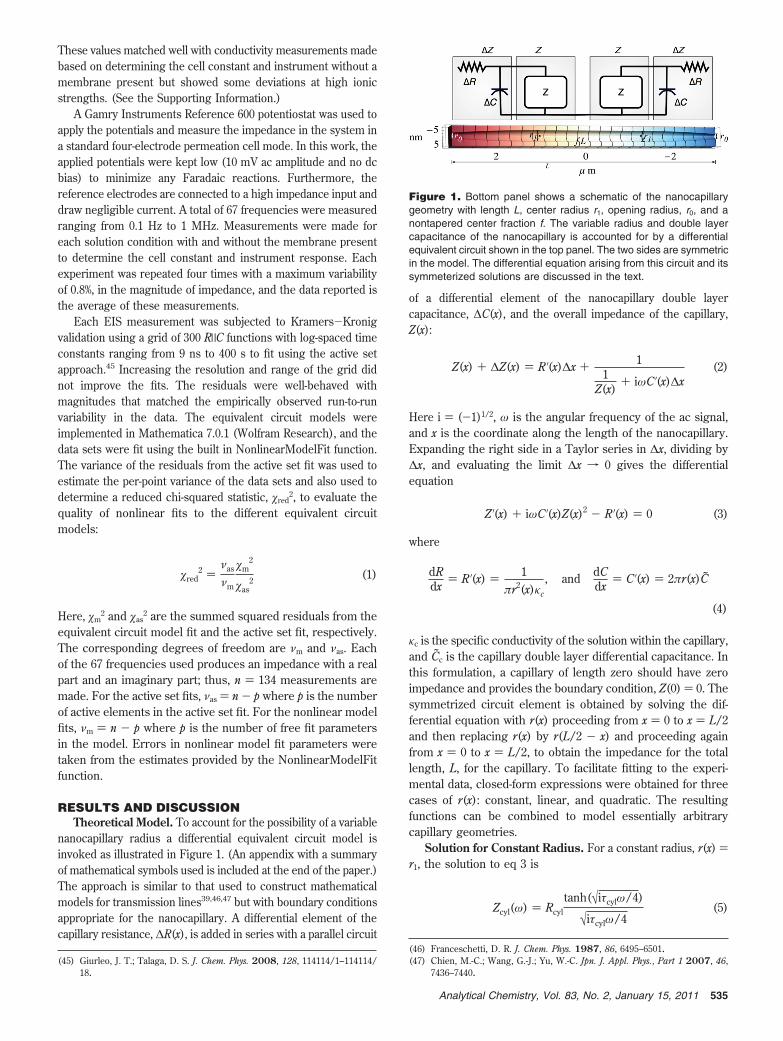
RESULTS AND DISCUSSIONTheoretical Model. To account for the possibility of a variable

nanocapillary radius a differential equivalent circuit model isinvoked as illustrated in Figure 1. (An appendix with a summaryof mathematical symbols used is included at the end of the paper.)The approach is similar to that used to construct mathematicalmodels for transmission lines39,46,47 but with boundary conditionsappropriate for the nanocapillary. A differential element of thecapillary resistance, ∆R(x), is added in series with a parallel circuit

of a differential element of the nanocapillary double layercapacitance, ∆C(x), and the overall impedance of the capillary,Z(x):

Z(x) + ∆Z(x) ) R'(x)∆x + 11

Z(x)+ iωC'(x)∆x

(2)

Here i ) (-1)1/2, ω is the angular frequency of the ac signal,and x is the coordinate along the length of the nanocapillary.Expanding the right side in a Taylor series in ∆x, dividing by∆x, and evaluating the limit ∆x f 0 gives the differentialequation

Z'(x) + iωC'(x)Z(x)2 - R'(x) ) 0 (3)

where

dRdx

) R'(x) ) 1πr2(x)κc

, and dCdx

) C'(x) ) 2πr(x)C

(4)

κc is the specific conductivity of the solution within the capillary,and Cc is the capillary double layer differential capacitance. Inthis formulation, a capillary of length zero should have zeroimpedance and provides the boundary condition, Z(0) ) 0. Thesymmetrized circuit element is obtained by solving the dif-ferential equation with r(x) proceeding from x ) 0 to x ) L/2and then replacing r(x) by r(L/2 - x) and proceeding againfrom x ) 0 to x ) L/2, to obtain the impedance for the totallength, L, for the capillary. To facilitate fitting to the experi-mental data, closed-form expressions were obtained for threecases of r(x): constant, linear, and quadratic. The resultingfunctions can be combined to model essentially arbitrarycapillary geometries.

Solution for Constant Radius. For a constant radius, r(x) )r1, the solution to eq 3 is

Zcyl(ω) ) Rcyl

tanh(√iτcylω/4)

√iτcylω/4(5)

(45) Giurleo, J. T.; Talaga, D. S. J. Chem. Phys. 2008, 128, 114114/1–114114/18.

(46) Franceschetti, D. R. J. Chem. Phys. 1987, 86, 6495–6501.(47) Chien, M.-C.; Wang, G.-J.; Yu, W.-C. Jpn. J. Appl. Phys., Part 1 2007, 46,

7436–7440.

Figure 1. Bottom panel shows a schematic of the nanocapillarygeometry with length L, center radius r1, opening radius, r0, and anontapered center fraction f. The variable radius and double layercapacitance of the nanocapillary is accounted for by a differentialequivalent circuit shown in the top panel. The two sides are symmetricin the model. The differential equation arising from this circuit and itssymmeterized solutions are discussed in the text.

535Analytical Chemistry, Vol. 83, No. 2, January 15, 2011

Equation 5 has the same functional form, but different parametri-zation, as the finite Warburg impedance.48-50 Equation 5 can beused to fit the geometry of a cylindrical nanocapillary and hastwo free parameters for fitting: the dc resistance, Rcyl, and a timeconstant, τcyl. Rcyl and τcyl have different dependencies onnanocapillary geometry, nanocapillary double layer differentialcapacitance, and solution conductivity given by

Rcyl )L

πr12κc

(6a)

τcyl ) RcylCcyl )2L2Cc

r1κc(6b)

Changes in the aspect ratio of the nanocapillary for a constantRcyl change the peak frequency in the Nyquist plot, which isobtained by maximizing - Im[Zcyl(ω)] from eq 5 giving

ωpeak ≈ 2.54/τcyl (7)

By altering the aspect ratio, the capillary surface area is changed.As the surface area increases the overall capacitance of thecapillary increases, which increases the time constant andconsequently decreases the peak frequency, eq 7. The net effectis a rescaling of the dependence of the spectrum on frequency,an effect best visualized in the plot of the imaginary componentof the impedance versus frequency as shown in Figure 2. Scalechanges of the parametric variable in parametric plots (e.g., aNyquist plot) appear as points that shift along a common curve.For a given dc impedance, (Rcyl), the peak frequency in theimaginary impedance plot tracks changes in total capillarydouble layer capacitance while the line shape remains constant.Thus, EIS can distinguish the capillaries aspect ratio based onthe peak frequency.

Solution for Linearly Varying Radius. Constriction at thenanocapillary opening results in a lozenge shape, and constriction

at the center results in an hourglass shape. Both of theses casescan be treated with a linearly varying capillary radius:

r(x) ) r0 + 2x(r1 - r0)/L (8)

where r0 is the entrance radius and r1 is the center radius.Integrating eq 3 using eq 8 gives a variation of the Warburgimpedance, referred to as the variable topology finite Warburgimpedance or ZVTW(ω) in this paper for arbitrary geometries.The linear case gives a closed form for lozenge shaped poresand capillaries.

Zloz(ω) )Rloz(I1(1)K1(0) - I1(0)K1(1))

τ1 - τ0×

( τ1

0(I2(0)K1(1) + I1(1)K2(0))+

τ0

1(I2(1)K1(0) + I1(0)K2(1)))(9)

where In is the modified Bessel function of the first kind oforder n and Kn is the modified Bessel function of the secondkind of order n. Also with

Rloz )L

κcπr1r0(10)

and

0 ) √i4τ0ω and 1 ) √i4τ1ω (11)

where

τ0 )L2Ccr0

2κc(r1 - r0)2 and τ1 )

L2Ccr1

2κc(r1 - r0)2

(12)

The ratio of the time constants is equal to the ratio of the entranceradius and center radius.

τ1

τ0)

r1

r0(13)

Complete details on the derivation of eq 9 are presented in theSupporting Information.

Figure 3 shows the predicted effect of constricting the capillaryopening on the EIS data. Capillaries with different degrees ofconstriction can give the same dc impedance and similar peakfrequencies. However, the magnitude of the imaginary componentof the EIS data is reduced across the peak as the degree ofconstriction increases. The time response of the differentialimpedance element is position-dependent because the relativevalues of the resistance and capacitance change along the lengthof the capillary. The changing radius introduces dispersion in thecharacteristic time constants of the circuit. In this representativeexample, the net effect of introducing new time scales to theresponse is to suppress the peak of the spectrum in the Nyquistplot. This effect increases with the degree of constriction of theopenings or the center.

(48) Warburg, E. Ann. Phys. 1899, 67, 493–499.(49) Macdonald, J. R. J. Chem. Phys. 1974, 61, 3977–3996.(50) Franceschetti, D. R.; Macdonald, J. R.; Buck, R. P. J. Electrochem. Soc. 1991,

138, 1368–1371.

Figure 2. Negative imaginary component of the EIS spectrum givesdifferent peak frequencies depending on the nanocapillary cylindricalaspect ratio r/L. Plots of eq 5 for the same values of Rcyl but differentaspect ratios are shown. The aspect ratios labeled in the figure arerelative to the reference geometry of L ) 6 µm, r ) 5 nm with κc )0.4 S/m, Cc ) 1.5 mF/m2.


Extension of ZVTW to Other Geometries. Nanopores andnanocapillaries may have many geometries20 that do not adhereto the simple assumptions of the cylindrical and linear constric-tions discussed thus far. The general nature of the variabletopology formalism allows determination of an equivalent circuitelement for essentially arbitrary geometries by rewriting thedifferential resistance and capacitance in eq 4. For example,extending the linear ZVTW function to a cone can be ac-complished simply by letting L be 2L in eq 9, and dividing by2. To accommodate quadratic changes in capillary radius as afunction of length, simply defining r(x) ) r0 + 4r1x2/L2 in eq 4and solving eq 3 leads to a closed form expression for ZVTW

involving Legendre functions (see the Supporting Information).Finally, the different ZVTW circuit elements can be combinedpiecewise to account for different regions of variable nanocap-illary radius. For example, the linear circuit element, Zloz, canbe combined with cylindrical circuit element, Zcyl, subject togeometric continuity constraints to model a tapered nanocap-illary that has a cylindrical center of fractional length f such atthat illustrated in Figure 1. The tapered capillary is modeled asthe sum of two circuit elements:

ZVTW ) Zcyl + Zloz (14)

the cylindrical center portion of length fL in the center, eq 9, andtwo tapered regions of total length (1 - f)L, eq 5, as illustrated inFigure 1. Thus, in eq 6 L is replaced by fL, and in eqs 10 and 12 Lis replaced by (1 - f)L. Combining eqs 9 and 5 requires the constraintthat the cylindrical portion have the same radius as the end of theadjoining tapered region. The time constant for the cylindricalcontribution is now determined by the other time constants:

τcyl )4Rcyl

2τ1(τ0 - τ1)2

Rloz2τ0

2 (15)

This eliminates τcyl as a fit variable. More complicated geom-etries can be built up similarly.

NCAM EIS Consistent with ZVTW. Figure 4 shows the EISdata taken on the NCAM at different solution conductivities. The

data without blank subtraction (Figure 4A) is dominated by asemielliptical (suppressed semicircular) feature. A small featureaccounting for 1-2% of the total impedance appears at lowfrequency (below 200 Hz). This feature was larger when using alarger dc potential bias. This feature did not contribute to the blank(Figure 4B) suggesting that it is due to the membrane. A largerfeature at high frequency, visible as an up-turn in the Nyquistplot, can be removed by subtraction of the blank data set. Afterblank subtraction (Figure 4C), the high-frequency limit approachesa phase angle of -55° ± 2° for all cases considered.

NCAM EIS Equivalent Circuit Elements. Figure 3 illustratesthe response of a single nanocapillary in isolation, while measuredEIS data accounts for additional impedances arising from theeffects of the membrane and surroundings. The data shows threedistinct features attributable to the instrument response (highfrequency), the membrane (low frequency), and the nanocapil-laries in the membrane (main peak). The response of theinstrument and cell, background, were found to be well-modeledby a two-element equivalent circuit:

Zbk ) Rbk|Cbk (16)

where Zbk, Rbk, and Cbk, are, respectively, the impedance,resistance, and capacitance of the electrochemical cell andinstrument. Membrane surfaces have been observed to givelow-frequency dispersive responses in EIS.51 To prevent thisfeature from perturbing the fit of the main nanocapillaryresponse we model the low-frequency feature with a simple(Rms|Cms) equivalent circuit. This element accounts for less than2% of the overall circuit impedance.

NCAMs comprise a large number of capillaries running inparallel across a capacitive polymeric membrane. Adding theimpedance ZVTW for each of the N capillaries in parallel withthe membrane capacitance Cmem gives

Zsys )ZVTW

N|Cmem (17)

Therefore, the overall equivalent circuit model becomes

Zexp ) Zsys + Zbk + (Rms|Cms) (18)

NCAM EIS is Consistent with a Lozenge Geometry. In thissection, several models for the nanocapillary response are fit tothe experimental data. The number of fit parameters, degrees offreedom, and 2 appear in Table 1. The nanocapillary responsein eq 18 is represented by a single impedance element, ZVTW.

A simple electrolyte conductor through a capacitive membranegives a R|C circuit response. Treating a nanocapillary as aconducting element requires a single fit parameter in addition tothose that account for the membrane and measurement system.The fits to such a model were very poor (see the SupportingInformation) giving a value of red

2 ∼ 4500. This is to be expectedgiven that the blank-subtracted data in Figure 4C shows thatthe high-frequency region approaches a phase angle of -55° ±2° as opposed to the -90° phase angle value predicted by theR|C circuit. Similarly, the peak in the Nyquist plot of the data is

(51) Coster, H. G. L. Biophys. J. 1973, 13, 118–132.

Figure 3. Effect of constriction of the openings of cylindricalnanocapillaries on the EIS spectrum is shown by plotting eq 9 fordifferent ratios of the radii as shown in the figure legend. Each of thefour nanocapillaries has the same dc resistance and would in principlegive identical current-voltage curves in spite of having vastly differentshapes. The EIS shows a clear change with nanocapillary geometry.The parameters used are L ) 6 µm, r1 ) 5 nm, κc ) 0.4 S/m, Cc )1.5 mF/m2. The inset shows renderings of the nanocapillary shapescorresponding to the radii ratios labeled in the figure.


suppressed compared to the R|C circuit. The resistive element isnot sensitive to aspect ratio and constrictions. Therefore, thecapacitive double layer is a likely candidate for improving the fitssince models including it show qualitative features much closerto those of the data as eq 9 predicts and as Figure 3 shows.

Treating the nanocapillaries with the cylindrical model includ-ing double layer capacitance, eq 5, requires one additional fitparameter per local fit and improves the fits substantially withred

2 reduced by nearly 9-fold. However, the cylindrical modelwith double layer capacitance still does not capture the degreeof suppression of the peak in the Nyquist plot. (See theSupporting Information.)

The presence of constrictions in the nanocapillary is predictedto cause further suppression of the peak in the Nyquist plot asshown in Figure 3. Indeed when the eq 9 is used for thenanocapillary response, all the main features of the data arecaptured and red

2 is reduced further by a factor of 8.2.Nanowires grown in NCAMs have shown that NCAMs maybe tapered at the ends.52-57 Equation 9 implies that the taper isacross the entire capillary rather than just at the ends. Thisgeometry can be modeled using eq 14. This further reduces red

2

by a factor of 1.8. Since further geometric complexity is difficultto justify based on the present understanding of ion-tracketched nanocapillaries, the fits using eq 14 will be the basis forfurther analysis. The fits to the experimental data using eq 14are shown as lines in Figure 4. The fit parameters and errors aresummarized in Table 2.

Local Fits Reveal Global NCAM EIS Model. There are twotypes of parameters in the ZVTW impedance element. Geometricparameters such as r0, r1, N, and L should be independent ofthe electrolyte concentration. The capacitance of the doublelayer should depend on the electrolyte concentration. Thechanges in EIS with electrolyte concentration allows separationof these effects through a global analysis. Figure 5 shows plotsof combinations of the local parameters that allow extraction ofthe global dependence of the geometric and capacitive propertiesof the nanocapillaries.

Figrure 5A shows a plot of the combination of parameters thatisolates the effective capillary conductivity

κc )(τ0 + τ1)

2

τ1(Rlozτ0 + Rcylτ1)L

π(r0 + r1)2N

(19)

versus the bulk solution conductivity. The conductivity in thecapillary is observed to be linearly related to the bulk conductivity(κc ) κb + κ0) with (κ0 ) 0.105 ± 0.003 S/m). The slightly higherconductivity inside the nanocapillary is consistent with therequirement of additional charge to neutralize capillary surfacecharge.18 This effect is most noticeable for capillaries withdiameters comparable to the Debye length at a given electrolyteconcentration.24,26,58-60

Figure 5B shows a plot of the ratio of time constants which isrelated to the ratio of the entrance and center radii through eq13. The plot shows that the ratio of radii parameter has an averagevalue of 2.0 ± 0.1. Figure 5C shows a plot of the combination oflocal fit parameters that give the fraction of the nanocapillarylength that is cylindrical:

f )τ1Rcyl

τ1Rcyl + τ0Rloz(20)

Figure 5C shows that the cylindrical fraction parameter has anaverage value of 0.416 ± 0.009. Both of the geometric nanocapillaryparameters show a modest dependence of their values on theconductivity. In both cases the conductivity dependence is smallerthan the error in the parameters as propagated from the fitparameters. This small effect is likely due to the covariance of fitparameters in the local nonlinear fitting function.

(52) Schonenberger, C.; Van Der Zande, B. M. I.; Fokkink, L. G. J. Mater. Res.Soc. Symp. Proc. 1997, 451, 359–365.

(53) Riveros, G.; Gomez, H.; Schrebler, R.; Marotti, R. E.; Dalchiele, E. A.Electrochem. Solid-State Lett. 2008, 11, K19–K23.

(54) Motoyama, M.; Fukunaka, Y.; Sakka, T.; Ogata, Y. H.; Kikuchi, S.Proc.sElectrochem. Soc. 2006, 2004-19, 99–108.

(55) De Leo, M.; Pereira, F. C.; Moretto, L. M.; Scopece, P.; Polizzi, S.; Ugo, P.Chem. Mater. 2007, 19, 5955–5964.

(56) Leopold, S.; Schuchert, I. U.; Lu, J.; Toimil Molares, M. E.; Herranen, M.;Carlsson, J.-O. Electrochim. Acta 2002, 47, 4393–4397.

(57) Ferain, E.; Legras, R. Nucl. Instrum. Methods Phys. Res., Sect. B 2001, 174,116–122.

(58) Desgranges, C.; Delhommelle, J. Phys. Rev. E: Stat., Nonlinear, Soft MatterPhys. 2008, 77, 027701/1–027701/4.

(59) Schoch, R. B.; van Lintel, H.; Renaud, P. Phys. Fluids 2005, 17, 100604/1–100604/5.

(60) Tang, Y. W.; Szalai, I.; Chan, K.-Y. Mol. Phys. 2001, 99, 309–314.

Figure 4. Panel A shows markers for experimental EIS data on a NCAM at five different concentrations of phosphate-buffered NaCl that giveconductivities as indicated in the figure legend. Panel B shows the response of the cell and instrument for the same solution conditions. PanelC shows the response of just the membrane obtained by the subtraction of the instrument response from the data. Local fits using eqs 14 and16 and their difference are shown as solid lines in panels A-C, respectively. Details of the fitting are discussed in the text.

Table 1. Quality of Model Fits

model m2 × 103 p ν red

2

R|Cmem 7700 30 640 4500Zcyl|Cmem 860 35 635 500Zloz|Cmem 100 40 630 61local (Zloz + Zcyl)|Cmem 57 45 625 34global (Zloz + Zcyl)|Cmem 64 22 658 37active set 1.5 100 570 1.0


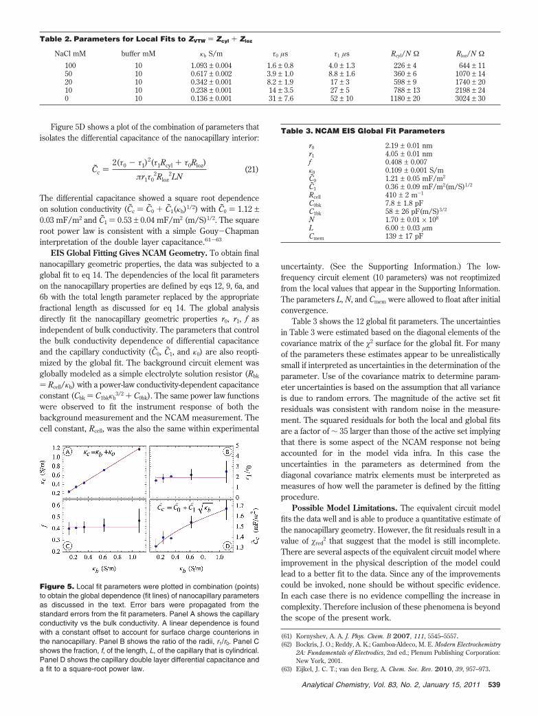
Figure 5D shows a plot of the combination of parameters thatisolates the differential capacitance of the nanocapillary interior:

Cc )2(τ0 - τ1)

2(τ1Rcyl + τ0Rloz)

πr1τ02Rloz

2LN(21)

The differential capacitance showed a square root dependenceon solution conductivity (Cc ) C0 + C1(κb)1/2) with C0 ) 1.12 ±0.03 mF/m2 and C1 ) 0.53 ± 0.04 mF/m2 (m/S)1/2. The squareroot power law is consistent with a simple Gouy-Chapmaninterpretation of the double layer capacitance.61-63

EIS Global Fitting Gives NCAM Geometry. To obtain finalnanocapillary geometric properties, the data was subjected to aglobal fit to eq 14. The dependencies of the local fit parameterson the nanocapillary properties are defined by eqs 12, 9, 6a, and6b with the total length parameter replaced by the appropriatefractional length as discussed for eq 14. The global analysisdirectly fit the nanocapillary geometric properties r0, r1, f asindependent of bulk conductivity. The parameters that controlthe bulk conductivity dependence of differential capacitanceand the capillary conductivity (C0, C1, and κ0) are also reopti-mized by the global fit. The background circuit element wasglobally modeled as a simple electrolyte solution resistor (Rbk

) Rcell/κb) with a power-law conductivity-dependent capacitanceconstant (Cbk ) C1bkκb

3/2 + C0bk). The same power law functionswere observed to fit the instrument response of both thebackground measurement and the NCAM measurement. Thecell constant, Rcell, was the also the same within experimental

uncertainty. (See the Supporting Information.) The low-frequency circuit element (10 parameters) was not reoptimizedfrom the local values that appear in the Supporting Information.The parameters L, N, and Cmem were allowed to float after initialconvergence.

Table 3 shows the 12 global fit parameters. The uncertaintiesin Table 3 were estimated based on the diagonal elements of thecovariance matrix of the 2 surface for the global fit. For manyof the parameters these estimates appear to be unrealisticallysmall if interpreted as uncertainties in the determination of theparameter. Use of the covariance matrix to determine param-eter uncertainties is based on the assumption that all varianceis due to random errors. The magnitude of the active set fitresiduals was consistent with random noise in the measure-ment. The squared residuals for both the local and global fitsare a factor of ∼ 35 larger than those of the active set implyingthat there is some aspect of the NCAM response not beingaccounted for in the model vida infra. In this case theuncertainties in the parameters as determined from thediagonal covariance matrix elements must be interpreted asmeasures of how well the parameter is defined by the fittingprocedure.

Possible Model Limitations. The equivalent circuit modelfits the data well and is able to produce a quantitative estimate ofthe nanocapillary geometry. However, the fit residuals result in avalue of red

2 that suggest that the model is still incomplete.There are several aspects of the equivalent circuit model whereimprovement in the physical description of the model couldlead to a better fit to the data. Since any of the improvementscould be invoked, none should be without specific evidence.In each case there is no evidence compelling the increase incomplexity. Therefore inclusion of these phenomena is beyondthe scope of the present work.

(61) Kornyshev, A. A. J. Phys. Chem. B 2007, 111, 5545–5557.(62) Bockris, J. O.; Reddy, A. K.; Gamboa-Aldeco, M. E. Modern Electrochemistry

2A: Fundamentals of Electrodics, 2nd ed.; Plenum Publishing Corporation:New York, 2001.

(63) Eijkel, J. C. T.; van den Berg, A. Chem. Soc. Rev. 2010, 39, 957–973.

Table 2. Parameters for Local Fits to ZVTW ) Zcyl + Zloz

NaCl mM buffer mM κb S/m τ0 µs τ1 µs Rcyl/N Ω Rloz/N Ω

100 10 1.093 ± 0.004 1.6 ± 0.8 4.0 ± 1.3 226 ± 4 644 ± 1150 10 0.617 ± 0.002 3.9 ± 1.0 8.8 ± 1.6 360 ± 6 1070 ± 1420 10 0.342 ± 0.001 8.2 ± 1.9 17 ± 3 598 ± 9 1740 ± 2010 10 0.238 ± 0.001 14 ± 3.5 27 ± 5 788 ± 13 2198 ± 240 10 0.136 ± 0.001 31 ± 7.6 52 ± 10 1180 ± 20 3024 ± 30

Figure 5. Local fit parameters were plotted in combination (points)to obtain the global dependence (fit lines) of nanocapillary parametersas discussed in the text. Error bars were propagated from thestandard errors from the fit parameters. Panel A shows the capillaryconductivity vs the bulk conductivity. A linear dependence is foundwith a constant offset to account for surface charge counterions inthe nanocapillary. Panel B shows the ratio of the radii, r1/r0. Panel Cshows the fraction, f, of the length, L, of the capillary that is cylindrical.Panel D shows the capillary double layer differential capacitance anda fit to a square-root power law.

Table 3. NCAM EIS Global Fit Parameters

r0 2.19 ± 0.01 nmr1 4.05 ± 0.01 nmf 0.408 ± 0.007κ0 0.109 ± 0.001 S/mC0 1.21 ± 0.05 mF/m2

C1 0.36 ± 0.09 mF/m2(m/S)1/2

Rcell 410 ± 2 m-1

C0bk 7.8 ± 1.8 pFC1bk 58 ± 26 pF(m/S)3/2

N 1.70 ± 0.01 × 108

L 6.00 ± 0.03 µmCmem 139 ± 17 pF


Though the ZVTW approach can accommodate a distributionof nanocapillary radii and/or shape, the current model doesnot include any contribution from nanocapillary geometricheterogeneity; it assumes all nanocapillaries have the samegeometry. Adding a distribution of geometries would increasethe dispersion of the time scales in the main EIS feature andwould lead to an improvement in the fit. However, ion-tracketched nanocapillaries are reported to be largely homogeneousin geometry.52,54,56 Attributing the dispersion of the nanocapillarycontribution to the EIS signal would imply a distribution ofcapillary cylindrical radii covering a range of ∼2.5 times theaverage radius. This is in significant excess of the specified andobserved distribution of ion-track etched nanocapillaries.

The range of time constants present in the componentattributed to the membrane could include contributions outsideof the low-frequency region that the equivalent circuit modelcurrently treats. The phenomenological treatment of these low-frequency contributions is descriptive and invokes serial R|Ccircuits. To resolve any possible overlap between these dispersivemembrane contributions to the EIS and the nanocapillary responsewould require a better phenomenological description than serialR|C circuits. Until such treatments are available this sort ofambiguity is likely to persist.

The geometry used to solve ZVTW and treat the nanocapillariesmay be too simplistic to represent the real nanocapillaries. Thepresent model exhibiting tapered ends with an approximatelycylindrical center is most complicated overall geometry thathas been confirmed to be present in NCAMs.52-57 Independentcharacterization of any variability of the nanocapillary radius isneeded to provide justification for additional geometric complexity.

The surface of the polycarbonate membrane is coated withpoly(vinylpyrrolidone). This detail is not distinguished in themodel. Given the thinness of the PVP passivation layer, it isunlikely that it would contribute significantly to the impedanceof the circuit.

The double layer differential capacitance is treated as a simpledifferential capacitor element.27 The actual response of the doublelayer is likely more complicated. It has been proposed touse multiple R|C components in order to separate the electricaldouble layer into the more diffuse Gouy-Chapman layer andinner, more compact Stern layer.38 Substitution of a morecomplicated model for the differential capacitor element wouldincrease the dispersion of ZVTW and possibly improve the fit.However, as with the other examples of added model complex-ity, there is no independent evidence to prefer this approachto improving the fit over the others already discussed.

Comparison of Fit Parameters and Manufacturer’s Speci-fications. The fit parameters suggest that the openings to thenanocapillaries are constricted by a factor of 1.85 from theircenters. Several imaging studies have shown that the nanocapil-laries are wider the middle as compared to the entrance andexit.52-57 The middle region of nanocapillaries can be wider thanthe entrance and exit by almost 3 times in some cases.52

The fit parameters indicate a nanocapillary entrance (and exit)radius of 2.19 ± 0.01 nm and a center radius of 4.05 ± 0.01 nm.The manufacturer reports the nominal radius to be 5 nm, with atolerance between 0 and -20% (or 4.5 ± 0.5 nm), a membranethickness of 6 µm with a tolerance of ±10%, and a capillary density

of 6 × 108 capillaries/cm2 with a tolerance of ±15%. Therefore,the fit parameter for the center radius is at the low end of themanufacturer’s specifications. The uncertainty in the membranethickness and nanocapillary number density together couldchange the estimated opening and center radii to be 2.49 and4.61 nm, respectively. Several additional phenomena couldaccount for a systematic underestimation of the nanocapillaryradii.

The mobility of ions in the electrical double layer is expectedto be reduced compared to those in the bulk. Such effects ofelectroviscosity25,64 are not explicitly incorporated into the model.It is possible that such an effect would increase the impedance ofthe nanocapillary. The net effect in fitting the present model wouldbe to underestimate the nanocapillary radii to compensate for theadded impedance. An improvement to the present model might,therefore, be to add a differential resistive element in series withthe double layer differential capacitive element. The low-frequencycomponent that was attributed to the membrane surface wasmodeled as a single R|C circuit. The active set fits indicated thatthis component was very dispersive in nature requiring six R|Ccomponents covering at least 4 decades in decay time. It ispossible that the membrane surface response also includedimpedance in the same spectral region as the nanocapillaries. Inthis case the additional impedance would manifest as a smallernanocapillary radius in the fitting.

Both the membrane thickness and capillary number densityare coupled in the fitting to the capillary geometry. If the thicknessof the membrane during the experiment is larger than thatspecified or if the number density of the nanocapillaries is lowerthan that specified, then the nanocapillaries radius will beunderestimated. Changing membrane thickness will also influencethe membrane capacitance. However, for changes in Cmem

consistent with the variability of the membrane thickness,essentially no changes were observed for the geometricparameters.

CONCLUSIONAn analytical modeling approach for extracting nanocapillary

geometry and double layer differential capacitance from EIS datahas been presented and validated experimentally through mea-surement on a commercial NCAM. By exploiting the differencesbetween the nanoscale and the bulk response to changes inelectrolyte concentration, the model provides a quantitativeestimate for the nanocapillary geometry. The methodology pre-sented in this work is expected to be of interest to the largercommunity of nanopore and nanocapillary investigators due tothe noninvasive nature of the technique.

ACKNOWLEDGMENTThis project was supported in part by award no. R01GM071684

from the National Institute of General Medical Sciences. Thecontent is solely the responsibility of the authors and does notnecessarily represent the official views of the National Instituteof General Medical Sciences or the National Institutes of Health.The authors thank the National Science Foundation for partialsupport of this work through Grant CBET 0813944. The authors

(64) Tas, N. R.; Haneveld, J.; Jansen, H. V.; Elwenspoek, M.; van den Berg, A.Appl. Phys. Lett. 2004, 85, 3274–3276.


thank Steve Dulin at GE Osmonics for valuable discussions ofthe NCAM properties.

Nomenclature List

Z impedance [Ω]R resistance [Ω]R′ dR/dx [Ω/m]C′ dC/dx [F/m]ω angular frequency [rad/s]i (-1)1/2 [ ]r radius [m]Cc capillary double layer differential capacitance [F/m2]κc capillary conductivity [S/m]κb bulk conductivity [S/m]L capillary length [m]Zcyl cylindrical impedance model [Ω]Zloz lozenge impedance model [Ω]ZVTW variable topology finite Warburg impedance [Ω]Rcyl resistance of a cylinder [Ω]Rloz resistance of a lozenge [Ω]r0 entrance (and exit) radius [m]r1 center radius [m]f fraction cylindrical length of nanocapillary [ ]τcyl time constant for constant radius capillary [s]τ0 time constant for r0 in Zloz [s]τ1 time constant for r1 in Zloz [s]Cmem membrane capacitance [F]N number of capillaries [ ]Amem membrane area [m2]Rms resistance of external membrane surface [Ω]Cms capacitance of external membrane surface [F]

Rbk cell and instrument resistance [Ω]Rcell cell constant [m-1]Cbk cell and instrument capacitance [F]C0bk constant coefficient in Cbk fit [F]C1bk κ3/2 coefficient in Cbk fit [F (m/S)3/2]Zbk cell and instrument impedance [Ω]Zexp experiment impedance [Ω]Zsys system impedance [Ω]κ0 increased capillary conductivity offset [S/m]C0 constant coefficient in Cc fit [F/m2]C1 square root coefficient in Cc fit [F/m2(m/S)1/2]ν degrees of freedom [ ]p number of fit parameters [ ]m

2 chi-squared model [Ω2]as

2 chi-squared active set [Ω2]red

2 reduced chi squared [ ]

SUPPORTING INFORMATION AVAILABLEA derivation of the ZVTW circuit element for cylindrical, lozenge,

conical, and quadratic geometries; the results of the active setfitting; the global fitting of the instrument response; the calibrationof the bulk conductivity and cell constant; the local fits to theexperimental data using R|Cmem, Zcyl|Cmem, and Zloz|Cmem; theparameters for the membrane surface and instrument responsefor the local fits to eq 14; the global fits of the data to eq 14; aschematic of the experimental setup. This material is available freeof charge via the Internet at http://pubs.acs.org.

Received for review August 25, 2010. Accepted November15, 2010.

AC102236K


Determining Nanocapillary Geometry from Electrochemical ......Determining Nanocapillary Geometry...

Documents

Transcript of Determining Nanocapillary Geometry from Electrochemical ......Determining Nanocapillary Geometry...