Determining landscape extent for succession and ...

RESEARCH ARTICLE

Determining landscape extent for successionand disturbance simulation modeling

Eva C. Karau Æ Robert E. Keane

Received: 9 May 2006 / Accepted: 27 January 2007 / Published online: 20 April 2007� Springer Science+Business Media B.V. 2007

Abstract Dividing regions into manageable

landscape units presents special problems in

landscape ecology and land management. Ideally,

a landscape should be large enough to capture a

broad range of vegetation, environmental and

disturbance dynamics, but small enough to be

useful for focused management objectives. The

purpose of this study was to determine the

optimal landscape size to summarize ecological

processes for two large land areas in the south-

western United States. We used a vegetation and

disturbance dynamics model, LANDSUMv4, to

simulate a set of nine scenarios involving system-

atically varied topography, map resolution, and

model parameterizations of fire size and fire

frequency. Spatial input data were supplied by

the LANDscape FIRE Management Planning

System (LANDFIRE) prototype project, an

effort that will provide comprehensive and scien-

tifically credible mid-scale data to support the

National Fire Plan. We analyzed output from

2,000 year simulations to determine the thresh-

olds of landscape condition based on the vari-

ability of burned area and dominant vegetation

coverage. Results show that optimal landscape

extent using burned area variability is approxi-

mately 100 km2 depending on topography, map

resolution, and model parameterization. Variabil-

ity of dominant vegetation area is generally

higher and the optimal landscape sizes are larger

in comparison to those features determined from

burned area. Using the LANDFIRE project as a

case study, we determined landscape size and

map resolution for a large mapping project, and

showed that optimal landscape size depends upon

geographical, ecological, and management con-

text.

Keywords Scale � Fire � Simulation modeling �Forest succession � Vegetation and disturbance

dynamics

Introduction

As interpretation of ecological processes and

patterns ultimately depends upon the scale of

analysis, the areal extent and spatial grain with

which we observe and quantify ecological systems

and conditions is of critical importance to land-

scape scale ecological studies (Allen and Starr

This paper was written and prepared by U.S. Governmentemployees on official time, and therefore is in the publicdomain and not subject to copyright. The use of trade orfirm names in this paper is for reader information and doesnot imply endorsement by the U.S. Department of Agri-culture of any product or service.

E. C. Karau (&) � R. E. KeaneUSDA Forest Service, Rocky Mountain ResearchStation Fire Sciences Laboratory, 5775 U.S. Highway10 West, Missoula, MT 59808, USAe-mail: [email protected]

123

Landscape Ecol (2007) 22:993–1006

DOI 10.1007/s10980-007-9081-y

1982; Wiens 1989). However, many studies fail to

identify appropriate landscape scale characteris-

tics for their projects. Others, out of necessity,

define the spatial extent and resolution of their

project by the extent and grain of available data

and then evaluate ecosystem characteristics with-

in that spatial domain (Mayer and Cameron

2003). Consideration of landscape scale is imper-

ative for ecological and land management issues

(Bailey et al. 1994; Bourgeron and Jensen 1994;

Tang and Gustafson 1997; White et al. 2000).

Indeed, many landscape ecological studies have

emphasized this matter and focused on identifi-

cation of landscape extents and spatial grains that

accurately characterize ecological patterns or

conditions using various methodologies including

semivariance analysis (Meisel and Turner 1998),

attractor reconstruction (Habeeb et al. 2005),

similarity indices (Baker 1989) and range of

variability (Wimberly et al. 2000).

Studies that address issues of landscape extent

tend to ask questions that are essential to land-

scape ecology, such as: ‘How big is a landscape?’

or ‘How large must an area be to function as a

landscape?’ (Forman and Godron 1986). This

depends on the landscape characteristic under

evaluation and the specific objective of the

analysis. For example a bark beetle’s (Coleoptera

Scolytidae) landscape might be intermediate in

size (3 km2) because callow adults fly about 1 km

after emergence, whereas a much larger land-

scape might be needed (102 or 103 km2) to study

fire patterns (Turner et al. 1995). However, what

if characteristics for defining a landscape were

many and broad (e.g., vegetation composition and

structure) and the context of evaluation vastly

complex (e.g., determining the historical range

and variability of all vegetation communities)?

Specifically, what would be the appropriate area

to evaluate changes in fire regime, vegetation

composition, and stand structure in a regional

context? It is difficult to determine an appropriate

landscape extent or ‘‘footprint’’ for summarizing

spatial attributes because interactions between

fire, vegetation succession, and biophysical set-

tings are complex and occur over several spatio-

temporal scales (Baker 1989). For example,

Wimberely et al. (2000) found that variation in

landscape attributes increased with decreasing

landscape extent. Clearly, landscape extent and

map resolution must be selected so that they

reflect the scale of the pattern forming processes

of interest (Fortin and Dale 2005).

The LANDFIRE project is charged with the

mapping of fire regime condition class (FRCC)

across the entire US (Rollins et al. 2006;

www.landfire.gov). FRCC is a three category

ordinal index that describes how far the current

landscape composition has departed from the

range and variation of historical conditions (Hann

2004) (see http://www.frcc.gov for complete de-

tails). However, the value of FRCC is strongly

scale dependent because it is greatly influenced by

the spatial extent and resolution of the data that

describes the ecological characteristics of the area

under evaluation. For example, the variability of

fire and vegetation area over time is often large for

relatively small evaluation areas (Li 2002). Con-

versely, if a fire management treatment area

comprised only a small portion of a large evalu-

ation area, then results of the treatment might be

undetectable. The LANDFIRE project needed to

determine a landscape extent that would be small

enough to detect subtle changes brought about by

land management, but large enough to reflect the

characteristic variability of important ecological

processes such as fire, succession, and biophysical

environment in the appropriate spatial context.

The challenge, then, was to identify an optimal

landscape size and an appropriate data grain with

which to summarize spatio-temporal dynamics of

important ecosystem characteristics such that

effects of management treatments and fires could

be determined in a context that was both mean-

ingful ecologically and applicable to land man-

agement planning. This study used simulation

modeling to explore the influence of landscape

extent and data resolution on the spatio-temporal

dynamics of important ecosystem characteristics,

such as fire size and vegetation succession class.

The primary objective was to determine optimal

landscape extent for summarizing ranges of his-

torical ecosystem conditions used in the compu-

tation of representative FRCC estimates over the

large regions mapped in the LANDFIRE project.

This study also evaluated the influence of simu-

lation parameters and model initialization on the

selection of the characteristic landscape extent.

994 Landscape Ecol (2007) 22:993–1006

123

http://www.frcc.gov

We initiated this study when the LANDFIRE

prototype project (Rollins et al. 2006) found that

to compute and map FRCC from the simulated

range of historical variation in landscape compo-

sition across large regional domains, it was

necessary to first define the size of the FRCC

mapping unit (Pratt et al. 2006). The variability

of simulated output was the metric that we used

to find the appropriate extent (spatial domain)

and resolution (pixel size) for describing simu-

lated time series of historical landscape compo-

sition. We define the ‘‘optimal’’ landscape extent

as the smallest spatial extent that minimizes the

influence of artificial variance due to landscape

size.

Background

The FRCC is an approximation of the departure

of current conditions from a simulated range of

historical conditions. The concept of historical

range of variability (HRV) serves as the founda-

tion to represent historical conditions in all FRCC

calculations (Landres et al. 1999; Swetnam et al.

1999; Keane et al. 2002a). In this study, HRV is

defined as the quantification of temporal and

spatial fluctuations of ecological processes and

characteristics prior to European settlement

(1900). The central assumption is that the quan-

tification of HRV can serve as an ecologically

meaningful reference for computing the depar-

ture (i.e. direction and magnitude of changes) of

current landscape structure and compositions

from historical trends. To use HRV in an oper-

ational context, it was necessary to select an

historical time span that best reflects the range of

conditions to use as reference for the manage-

ment of future landscapes; an assumption that

may be overly simplistic because of documented

climate change, exotic introductions, and human

land use (Hessburg et al. 1999, 2000). For this

study, we limited the temporal context of HRV to

the time span from circa 1600 AD to 1900 AD as

this period provides the historical data (fire scar

chronologies) necessary to quantify simulation

parameters.

HRV can be described from many ecological

characteristics, and in this study, we selected

landscape composition (percent abundance) as

the primary evaluation criteria. We describe

landscape composition as the area occupied by

the combination of the Potential Vegetation Type

(PVT) and succession class map units. A PVT

identifies a distinct biophysical setting that sup-

ports a unique and stable plant community in the

absence of disturbance under a constant climate

regime (Daubenmire 1966; Pfister and Arno

1980). The succession class is represented by a

combination of cover type (named for the dom-

inant plant species based on canopy cover) and

structural stage (defined by canopy cover and

height stratifications). Structural stages represent

linear progressions of stand development based

on the classification of O’Hara et al. (1996) where

low cover and height represent early successional

stages and high cover and height represent late

successional stages.

LANDSUMv4

The LANDscape SUccession Model (LAND-

SUMv4) was used to generate the simulated

HRV statistics. It is a C++ program wherein

vegetation development is simulated as a deter-

ministic process and disturbances are modeled as

stochastic, spatially explicit processes (Keane

et al. 1997). LANDSUMv4, the fourth major

revision of the original LANDSUM, was devel-

oped to simulate the historical landscape dynam-

ics which quantify the historical range and

variation of landscape characteristics used to

calculate the FRCC (Keane et al. 1996, 2002b).

The model uses a spatial state-and-transition

succession approach where fire growth is simu-

lated with a cell percolation module. The first

LANDSUM was created by modifying the

CRBSUM model (Keane et al. 1996), implemented

at a 1 km pixel scale, to simulate succession at a

polygon level (1–100 ha) (Keane et al. 1997). A

spatially explicit fire spread algorithm was in-

cluded (LANDSUM version 2.0) to explore the

limitations and implications of using a simulation

approach to describe landscape dynamics (Keane

et al. 2002b). A simplistic climate driver was then

implemented to create LANDSUM version 3.0

(Cary et al. 2006). The LANDSUMv4 version

contains extensive refinements to the fire spread

Landscape Ecol (2007) 22:993–1006 995

123

and successional development algorithms (e.g.,

improved ignition simulation, climate driver, and

multiple effects pathways for a single distur-

bance) and options for generating historical time

series information for LANDFIRE (e.g., fire atlas

layers, a list of all fires and an output format

compatible with statistical software) (Keane et al.

2006).

LANDSUMv4 simulates succession within a

polygon (adjacent similar pixels) using the multi-

ple pathway fire succession modeling approach

presented by Kessell and Fischer (1981) and

based on the seminal works of Noble and Slatyer

(1977), and Davis et al. (1980). This approach

assumes all pathways of successional develop-

ment will eventually converge to a stable or quasi-

climax plant community (PVT) (Fig. 1). There is

a single set of successional pathways for each

PVT present on a given landscape (Arno et al.

1985). Successional development within a poly-

gon is simulated as a change in successional class

(cover type-structural stage doublet) at an annual

time step. The length of time a polygon remains

in a succession class (transition time-years) is an

input parameter that is held constant throughout

the simulation. Disturbances disrupt succession

and can delay or advance the time spent in a

succession class, or cause an abrupt change to

another succession class. Occurrences of human-

caused and natural disturbances are stochastically

modeled from input probabilities based on his-

torical frequencies. All disturbances are simu-

lated at a polygon level, except for wildland fire,

which is spread across the landscape at a pixel

level using a spatial cell automata. Fire is spread

cell-to-cell based on vectors of slope (derived

from an input digital elevation model, DEM) and

wind (average speed and direction are input

parameters) until it reaches a stochastically

determined fire size calculated from an exponen-

tial function of fire size parameterized from

average fire size inputs (Keane et al. 2002a). For

full documentation of all LANDSUMv4

algorithms, along with model sensitivity and

behavior analyses, see http://www.fs.fed.us/rm/

pubs/rmrs_gtr171.pdf.

Fig. 1 A simplistic succession pathway in LANDSUMv4where cover type and structural stage categories arelinked along pathways of successional development basedon shade tolerance. The terminal cover type (SF) is thePotential Vegetation Type (PVT) category because itrepresents the most shade tolerant tree species. Covertype names are as follows: mountain shrub (SH),

whitebark pine (WP), subalpine fir (SF). Structural stagenames are defined as: low cover low height (LCLH) earlysuccession stage, high cover low height mid-seral stage(HCLH), high cover high height late succession stage(HCHH), low cover high height (LCHH) disturbancemaintained late succession stage. T1-11 identify uniquesuccession classes

996 Landscape Ecol (2007) 22:993–1006

123

Methods

Study areas

We implemented this study on two large land-

scapes (each approximately 75 · 75 km2) chosen

from within mapping Zone 16 of the LANDFIRE

prototype project area (Fig. 2) (see Rollins et al.

2006 for more detailed information). Mapping

zones were developed by the Earth Observation

and Science (EROS) Data Center (http://

www.nationalmap.gov). They are broad biophys-

ical land units represented by similar surface

landforms, land cover conditions, and natural

resources; there are 66 in the continental U.S. The

‘mountainous’ landscape is situated in north

central Utah’s Uinta Mountains and the ‘flat’

landscape encompasses the town of Manti in the

south central part of the state. These landscapes

were selected to represent two large regions that

differ in geography, topography, and ecology, but

still lie within the same mapping zone.

The mountainous landscape is dominated by

temperate coniferous forests of ponderosa pine

(Pinus ponderosa) and Douglas-fir (Pseudotsuga

menziesii) at lower elevations and lodgepole pine

(P. contorta), subalpine fir (Abies lasiocarpa), and

spruce (Picea spp.) at higher elevations. A spruce-

fir cover type makes up just over 25% of the

mountainous landscape, while other dominant

cover types are: lodgepole pine (19%), aspen-birch

(16%), and mountain big sagebrush (Artemesia

Tridentata vaseyana) (12%). The following cover

types each occupy between 1% and 5% of

the mountainous landscape: Douglas-fir, pinyon-

juniper, Wyoming Basin big sagebrush (A. t.

Fig. 2 The twosimulation landscapes, flatand mountainous, shownwithin mapping Zone 16of the LANDFIREprototype project

Landscape Ecol (2007) 22:993–1006 997

123

wyomingensis), dwarf sagebrush (A. t. scopulorum),

mountain deciduous shrub, riparian shrub, cool-

season perennial grasslands, and open water.

Barren and alpine environments on the ridges

and high peaks of the Uintas cover about 9% of

total mountainous landscape area. Though the

mountainous landscape terrain primarily features

steep topography, it includes areas that are hilly,

undulating and flat.

The flat landscape is primarily comprised of

cover types that tend to occur at low elevation in

flat to rolling terrain; pinyon or pinyon-juniper

covers over 30% of the landscape and each of the

following cover types occupy between 5% and

10%: salt desert shrub, mountain deciduous

shrub, Wyoming basin big sagebrush complex

and agriculture. Mountain big sage, dwarf sage,

rabbitbrush (Chrysothamnus nauseosus), peren-

nial grasslands, urban, barren and open water

cover types each occupy between 1% and 5% of

the flat landscape. Because Utah topography is so

diverse and the simulated landscape so large

(over 5,500 km2), it was impossible to center the

nested landscape box on an area that was entirely

flat. Consequently, grand fir (A. grandis), spruce-

fir and aspen (Populus tremuloides) vegetation

types, situated in small areas of foothills and

mountains, cover between 5% and 10% of the flat

landscape’s total extent.

Model initialization and parameterization

The LANDSUMv4 input data layers required for

this study were developed by the LANDFIRE

prototype project. The DEM layer was taken

from the National Elevation Dataset (http://

www.nationalmap.gov). Creation of the input

PVT map (Fig. 3) involved a supervised classifi-

cation of an extensive field plot database and

spatial modeling of over 50 biophysical data

layers (Frescino et al. 2006). The cover type and

structural stage layers for current conditions were

developed from an integration of Landsat 7 ETM

satellite imagery with the 50 biophysical layers

LandscapeSimulation Units (km2)

13.0

20.3

51.8

0.8

3.2

116.6

1049.8

2540.2

5055.2

5944.4

Potential Vegetation Type

Agricultural

Alpine

Aspen

Barren

Blackbrush

Cool Herbaceous

Dwarf Sagebrush

Grand Fir- White fir

Lodgepole Pine

Mountain Big Sagebrush

Open Water

Ponderosa Pine

Riparian Hardwood

Riparian Shrub

Salt Desert Shrub

Snow - Ice

Spruce Fir- Blue Spruce

Timberline Pine

Urban - Developed

Warm Herbaceous

Wetland Herbaceous

WY-Basin Big Sagebrush

Pinon Juniper

Douglas-fir

Fig. 3 The nested set ofsimulation reporting unitscentered on the flatlandscape and draped onthe LANDFIRE Zone 16Prototype PotentialVegetation Type map.The same set of ninenested landscape sizeswas used for themountainous landscape

998 Landscape Ecol (2007) 22:993–1006

123

(Zhu et al. 2006). All input layers were developed

at 30 m spatial resolution for the entire mapping

zone (Fig. 2). Considering that previous studies

evaluated LANDSUMv4 behavior and sensitivity

and found that the initial landscape had no effect

on simulated conditions after 300–500 years of

simulation (Keane et al. 2002b, 2006; Pratt et al.

2006), we created initial conditions for the

succession class map in the LANDSUMv4 simu-

lations by assigning the most dominant succession

class for each PVT across the landscape.

The LANDSUMv4 model was parameterized

using the fire and succession information com-

piled by the LANDFIRE team for Zone 16

(summarized in Table 1, but see Long et al. 2006

for details). As mentioned, LANDSUMv4 was

parameterized for LANDFIRE to simulate

historical conditions representative of the

1600–1900 AD time span. Succession transition

times were taken from extensive literature

searches and stand development data, historical

fire frequencies from fire history studies con-

ducted within the general mapping zone, and fire

size distributions from data compiled by Schmidt

et al. (2002) which incorporates the National

Interagency Fire Management Integrated Data-

base (NIFMID) database and local fire records.

Simulation scenarios

The simulation design comprised nine nested

reporting units selected to represent a range of

landscape extents from very small (approximately

1 km2) to very large (over 5,000 km2), each sized

to allow cells from four map resolutions to fit

perfectly within box boundaries (Fig. 3). Around

the largest landscape reporting unit we added a

3 km wide buffer to minimize edge effects and

ensure that fires burn realistically into the largest

landscape (Keane et al. 2001; Pratt et al. 2006).

Simulated burned area and dominant vegetation

area results were output from LANDSUMv4 for

each of the reporting unit landscapes across the

2000 year simulation interval.

We included four levels of landscape resolution

in our study design to investigate the effect of

spatial grain on optimal landscape extent. We

aggregated the original 30 m resolution land-

scapes by assigning the mean elevation value

and modal PVT value to the three coarser

resolution grids (90, 300 and 900 m per side).

When the landscape size is 0.81 km2 and land-

scape resolution is 900 m, only one pixel defines

the entire reporting area.

Because disturbance frequencies and size dis-

tributions ultimately influence landscape compo-

sition over time (Turner et al. 1993), we varied

Table 1 Summary of key parameters used for the two simulation areas in the LANDSUMv4 simulations for the three mostcommon potential vegetation types (PVT)

Most common PVT Average fireprobability

Averagetransition time(years)

Number ofsuccessionalclasses*

Initial successionalclass*

Mountainous landscape (33 PVTs)Spruce fir 0.00755 31 40 Spruce-fir HCHHMountain big sagebrush 0.04850 17 10 Mountain big sagebrush complex

HCLHRiparian shrub 0.00875 9 4 Riparian shrub HCHHFlat landscape (31 PVTs)Wyoming-basin big sagebrush 0.01257 45 11 Wyoming-basin big sagebrush

complex LCLHPinyon-junipe/Wyoming-basin

big sagebrush0.01396 32 20 Juniper LCLH

Pinyon-juniper/mountainbig sagebrush

0.02587 28 18 Juniper LCLH

For full documentation of model parameters, see Long et al. (2006)

* Successional Class is represented by a combination of cover type and structural stage combination. Here, structural stageis abbreviated using a combination of four letters: C = Cover (%), H = height (m), L = low, H = high. For example,HCLH = High Cover Low Height

Landscape Ecol (2007) 22:993–1006 999

123

LANDSUMv4 fire parameters to quantify the

effect of disturbance on the optimal landscape

size, again using the burned area and vegetation

composition time series. Two LANDSUMv4

parameters describe fire dynamics in any simula-

tion: average fire size and fire ignition probability.

We chose three levels of average fire size (0.01,

0.30 and 10.0 km2) to represent a range of sizes

for regions across the United States. The histor-

ical fire ignition probabilities quantified by the

LANDFIRE prototype project represented the

reference or historical fire probability set and

they are quantified for every PVT-succession

class combination input by the user. We then

created another set of fire probabilities that were

half the historical parameters (Table 1) and a

third set that was double the historical parame-

ters. We expected higher variance for simulations

that had larger fires or more frequent fires

because more area would be burned each simu-

lation year.

We ran the LANDSUMv4 landscape fire

succession model for each of the 72 factor

permutations of topography (flat and mountain-

ous), spatial grain (pixel sizes: 30, 90, 300 and

900 m per side), average fire size (0.01, 0.3, and

10.0 km2), and ignition probability (half histori-

cal, historical, and double historical). LAND-

SUMv4 will only simulate a fire in a pixel if the

fire size is greater than half the size of the pixel, so

no output was generated for the factor combina-

tion 900 m resolution, 0.81 km2 reporting unit,

and 0.01 km2 average fire. Results were summa-

rized for nine landscape extents: 0.81, 3.2, 13.00,

20.30, 51.80, 116.60, 1,049.80, 2,540.20, and

5,055.30 km2. A 3 km buffer surrounds the largest

extent and brings the total area of the simulation

landscape to 5,944.4 km2 (Fig. 3).

To minimize the effect of initial conditions, we

ran the model for a 500 year spin-up period

before printing the first year of output, then

burned area and dominant PVT-succession class

area were output for each landscape size (nine

reporting units) every 20 years thereafter for a

total of 2,000 years. This yielded 100 data points

per factor combination. Our choice of the

2,000 year simulation length and 20 year report-

ing interval allowed us to obtain enough data

points to avoid temporal autocorrelation while

minimizing lengthy simulation times (Keane et al.

2002b; Pratt et al. 2006). Exceptionally long

model simulation times for the 30 m input layers

precluded study replication (the 30 m resolution

simulation sets each ran for over 1 month, 90 m

resolution sets ran for approximately one week,

and the 300 and 900 m resolution less than 1 day).

We used two diagnostic variables to determine

optimal landscape extent from the set of report-

ing units: (1) ln(rba2 ), representing the natural log

of variation throughout the simulation interval of

the percent of each reporting unit area burned by

fire and (2) ln(rvg2 ), representing the natural log of

variation of the percent of each reporting unit

area occupied by the PVT-succession class com-

bination that is present on all of the nested

landscape reporting units; Wyoming Basin Big

Sage (High Cover, Low Height) for the flat

landscape, and Spruce-Fir (Low Cover, High

Height) for the mountainous. The notation

ln(r2) refers to both ln(rba2 ) and ln(rvg

2 ).

We chose to look at the variation of these

factors because quantification of historical range

and variation is important for landscape scale fire

regime studies. We reasoned that until the land-

scape size is large enough that there is no longer a

change in variance of the response variable

(variance reaches a plateau when plotted against

increasing reporting unit size), measurement

accuracy will be compromised because values

will be influenced by variation due to the size of

the landscape rather than due only to natural

fluctuations in the factor of interest.

To graphically summarize relative differences

in variance between fire size, fire frequency and

landscape resolution permutations, we plotted

variance for all factor combinations through the

range of landscape extents (Figs. 4, 5). Because

there was a large range in raw variance values, we

used a natural log transformation to mathemat-

ically compress the range of the data so that

variance curves could be shown on the same

charts. Also for display purposes, we truncated

the curves to show only the first six landscape

sizes, as the lines were generally flat through the

largest landscape extents and the optimal land-

scape size was always under 500 km2.

To determine optimal landscape size, ln(rba2 )

and ln(rvg2 ), were evaluated across the range of

1000 Landscape Ecol (2007) 22:993–1006

123

landscape sizes to locate the landscape reporting

unit where the ln(r2) approaches an asymptote.

We assumed that this point identified the land-

scape size where the variability of simulated

diagnostic variables is least affected by the size

of the reporting unit, so choosing a reporting unit

of this size (or larger) to summarize simulated fire

regime variables will minimize artificial variance.

The curve fitting method that we used, a third

order polynomial interpolation, consistently pro-

duced the best fit through our ln(r2)-landscape

size points. For a consistent and repeatable

measurement, and to account for slight deviations

from the general shape trend in a few of the

curves, we defined the asymptote as the point

where the slope of the interpolated curve first

exceeds 0.005 percent2 km–2 (a 0.5% or 0.29�

angle). The corresponding x-axis value was then

taken as the optimal landscape extent.

Results

The majority of the ln(r2)-landscape size curves

had a shape defined by very large ln(r2) values for

small landscapes (~0–50 km2), steep drops in

ln(r2) in the intermediate landscape extents

(~50–200 km2), and a plateau after extents larger

than approximately 200 km2. There were slight

deviations from this trend in a few of the curves

due to greater variety of PVT-succession class

combinations at large landscape sizes. Note that

there are no results for the 0.01 km2 average fire

size in the 900 m resolution case, as the model

-4

-2

0

2

4

6

8

0 100 200 300

-4

-2

0

2

4

6

8

0 100 200 300

-4

-2

0

2

4

6

8

0 100 200 300

-4

-2

0

2

4

6

8

0 100 200 300

-4

-2

0

2

4

6

8

0 100 200 300

-4

-2

0

2

4

6

8

0 100 200 300

-4

-2

0

2

4

6

8

0 100 200 300

-4

-2

0

2

4

6

8

0 100 200 300

-4

-2

0

2

4

6

8

0 100 200 300

-4

-2

0

2

4

6

8

0 100 200 300

-4

-2

0

2

4

6

8

0 100 200 300

-4

-2

0

2

4

6

8

0 100 200 300

-4

-2

0

2

4

6

8

0 100 200 300

Increasing Fire Ignition Probability

half historical double

Increas ingA

ver ageF

ireS

ize

30m 90m 300m 900m


Mountainous LandscapeFlat Landscape


3.0

0.0101

3.0

0.0101

cnI

gni

s aer

egar

evA

zei

S er i

F

Landscape Size (km2)






-4

-2

0

2

4

6

8

0 100 200 300

-4

-2

0

2

4

6

8

0 100 200 300

-4

-2

0

2

4

6

8

0 100 200 300

(nlσ

ab)

2(nlσ

ab)

2(nlσ

ab)

2

(nlσ

ab)

2(nlσ

ab)

2(nlσ

ab)

2

-4

-2

0

2

4

6

8

0 100 200 300

-4

-2

0

2

4

6

8

0 100 200 300

Fig. 4 ln(rba2 ) versus landscape size for the flat and

mountainous landscapes. The three fire ignition probabil-ities (half, historical and double) are arranged in columnsand the three average fire sizes (0.01, 0.3, and 10 km2) in

rows. As the curves remain quite flat for the largestlandscapes, the x-axes are truncated to show only the firstsix landscapes

Landscape Ecol (2007) 22:993–1006 1001

123

only ignites a fire in a pixel if the fire size is

greater than half of the pixel size.

The relationship of ln(rba2) to landscape size

is similar for both topographic types (flat and

mountainous) across all landscape resolutions

(Fig. 4) with the coarsest resolutions displaying

the highest values. This relationship is also

apparent for ln(rvg2 ), through the range of

landscape sizes (Fig. 5). For both flat and

mountainous landscapes, the 900 m resolution

simulation exhibited the highest ln(r2) and the

highest optimal landscape sizes. Interestingly,

there is very little difference between the 30,

90, and 300 m pixel resolution simulation ln(r2)

curves for both burned area and vegetation

class and for a number of landscape sizes and

landscape types. The 30 and 90 m curves are

particularly similar, while the coarser resolution

curves (300 m) and especially the 900 m curves

displayed notably higher magnitudes of ln(r2)

(Figs. 4, 5).

LANDSUMv4 simulations with LANDFIRE

historical fire regime parameterizations at 30 m

resolution (simulation design used by the

LANDFIRE project) produced ln(rba2 ) results

that appear to approach an asymptote when the

landscape reporting area is between 80 km2 and

100 km2 for both the flat and mountainous

landscape types (Fig. 4). Indeed the specific

optimal landscape for these simulation sets were

84 km2 for the flat and 90 km2 mountainous

topographic types (Table 2). The ln(rvg2 ) curve

flattened further along the landscape size axis

(Fig. 5) and the optimal landscape sizes were 106

and 112 km2 for the flat and mountainous land-

scapes respectively (Table 3).

-4

-2

0

2

4

6

8

0 100 200 300

-4

-2

0

2

4

6

8

0 100 200 300

-4

-2

0

2

4

6

8

0 100 200 300

-4

-2

0

2

4

6

8

0 100 200 300

-4

-2

0

2

4

6

8

0 100 200 300

-4

-2

0

2

4

6

8

0 100 200 300

-4

-2

0

2

4

6

8

0 100 200 300

-4

-2

0

2

4

6

8

0 100 200 300



Increas ing Aver age F

ire Size

30m 90m 300m 900m


Mountainous LandscapeFlat LandscapeIncreasing Fire Ignition Probability

0.30.01

10

0.30 .0 1

10Inc reasing A

verage Fire S

iz e







ln(σ

vg)

2ln

(σvg

)2

ln(σ

vg)

2

ln(σ

vg)

2ln

(σvg

)2

ln(σ

vg)

2

-4

-2

0

2

4

6

8

0 100 200 300

-4

-2

0

2

4

6

8

0 100 200 300

-4

-2

0

2

4

6

8

0 100 200 300

-4

-2

0

2

4

6

8

0 100 200 300

-4

-2

0

2

4

6

8

0 100 200 300

-4

-2

0

2

4

6

8

0 100 200 300

-4

-2

0

2

4

6

8

0 100 200 300

-4

-2

0

2

4

6

8

0 100 200 300

-4

-2

0

2

4

6

8

0 100 200 300

-4

-2

0

2

4

6

8

0 100 200 300

Fig. 5 ln(rvg2 ) versus landscape size for the flat and

mountainous landscape. The three fire ignition probabil-ities (half, historical and double) are arranged in columnsand the three average fire sizes (0.01, 0.3, and 10 km2) in

rows. As the curves remain quite flat for the largestlandscapes, the x-axes are truncated to show only the firstseven landscapes

1002 Landscape Ecol (2007) 22:993–1006

123

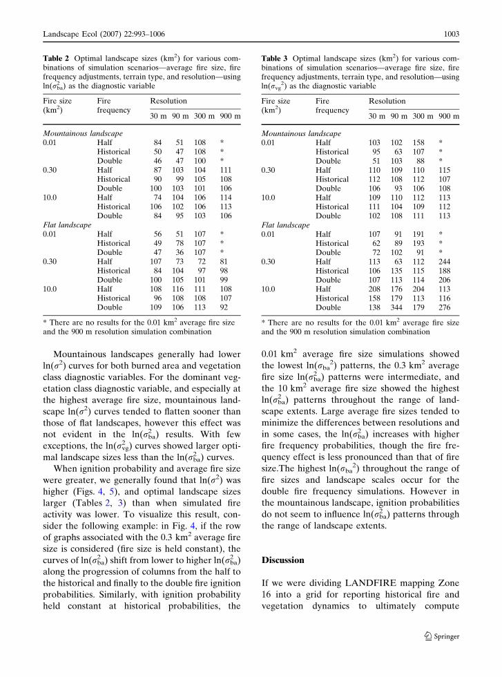
Mountainous landscapes generally had lower

ln(r2) curves for both burned area and vegetation

class diagnostic variables. For the dominant veg-

etation class diagnostic variable, and especially at

the highest average fire size, mountainous land-

scape ln(r2) curves tended to flatten sooner than

those of flat landscapes, however this effect was

not evident in the ln(rba2 ) results. With few

exceptions, the ln(rvg2 ) curves showed larger opti-

mal landscape sizes less than the ln(rba2 ) curves.

When ignition probability and average fire size

were greater, we generally found that ln(r2) was

higher (Figs. 4, 5), and optimal landscape sizes

larger (Tables 2, 3) than when simulated fire

activity was lower. To visualize this result, con-

sider the following example: in Fig. 4, if the row

of graphs associated with the 0.3 km2 average fire

size is considered (fire size is held constant), the

curves of ln(rba2 ) shift from lower to higher ln(rba

2 )

along the progression of columns from the half to

the historical and finally to the double fire ignition

probabilities. Similarly, with ignition probability

held constant at historical probabilities, the

0.01 km2 average fire size simulations showed

the lowest ln(rba2) patterns, the 0.3 km2 average

fire size ln(rba2 ) patterns were intermediate, and

the 10 km2 average fire size showed the highest

ln(rba2 ) patterns throughout the range of land-

scape extents. Large average fire sizes tended to

minimize the differences between resolutions and

in some cases, the ln(rba2 ) increases with higher

fire frequency probabilities, though the fire fre-

quency effect is less pronounced than that of fire

size.The highest ln(rba2) throughout the range of

fire sizes and landscape scales occur for the

double fire frequency simulations. However in

the mountainous landscape, ignition probabilities

do not seem to influence ln(rba2 ) patterns through

the range of landscape extents.

Discussion

If we were dividing LANDFIRE mapping Zone

16 into a grid for reporting historical fire and

vegetation dynamics to ultimately compute

Table 2 Optimal landscape sizes (km2) for various com-binations of simulation scenarios—average fire size, firefrequency adjustments, terrain type, and resolution—usingln(rba

2 ) as the diagnostic variable

Fire size(km2)

Firefrequency

Resolution

30 m 90 m 300 m 900 m

Mountainous landscape0.01 Half 84 51 108 *

Historical 50 47 108 *Double 46 47 100 *

0.30 Half 87 103 104 111Historical 90 99 105 108Double 100 103 101 106


Flat landscape0.01 Half 56 51 107 *




* There are no results for the 0.01 km2 average fire sizeand the 900 m resolution simulation combination

Table 3 Optimal landscape sizes (km2) for various com-binations of simulation scenarios—average fire size, firefrequency adjustments, terrain type, and resolution—usingln(rvg

2) as the diagnostic variable

Fire size(km2)

Firefrequency

Resolution

30 m 90 m 300 m 900 m

Mountainous landscape0.01 Half 103 102 158 *




Flat landscape0.01 Half 107 91 191 *




* There are no results for the 0.01 km2 average fire sizeand the 900 m resolution simulation combination

Landscape Ecol (2007) 22:993–1006 1003

123

FRCC, based on our results, we would select a

summary unit size between 50 km2 and 120 km2

(Figs. 4, 5; Tables 2, 3). The optimal landscape

extent would likely be larger if changes in

vegetation composition were important and

smaller if fire regimes, represented here by the

nine fire size-frequency scenarios, were empha-

sized in the analysis. The landscape reporting unit

sizes can be smaller for mountainous areas or for

regions that are topographically complex, but

must be larger when the region is flat and when

fires can become large. Mountainous landscapes

tend to have lower ln(r2) than flat landscapes,

especially at fine resolutions and when vegetation

is emphasized; coarse resolutions may be appro-

priate when fires are large in mountainous land-

scapes (Figs. 4, 5).

Simulation results from the 30 and 90 m

resolution landscapes were very similar in mag-

nitude and pattern of ln(r2) for all simulation

scenarios, indicating that simulations using 90 m

or even 300 m resolution landscapes may have

comparable quality to 30 m resolution. If coarser

resolutions are viable for large area applications

such as LANDFIRE, simulation and processing

time would be accelerated, with potentially small

losses in information content. This result is

fortuitous for cases where fine-grained data are

unavailable, but most importantly, coarse-grained

landscapes allow efficient simulation of larger

areas and longer time spans, allowing generation

of statistically stronger estimates of historical

ranges and variation of landscape characteristics.

There are a number of reasons why ln(rba2 )

differed from ln(rvg2 ). First, the magnitude of

burned area for each output reporting interval

was often less than the simulated dominant

vegetation class extent. Also, vegetation class will

change as a result of fire and successional devel-

opment, causing great diversity in vegetation class

area across output reporting intervals. Moreover,

a change in one vegetation class will always result

in a change in one or more other classes, thus

increasing ln(rvg2 ).

The LANDSUMv4 fire spread algorithm had a

great influence on the effects of resolution and

fire regime on variability and optimal landscape

size. Since fires will not ignite unless the com-

puted fire size is greater than half the pixel size,

coarser resolutions have few small fires because

many of the simulated fire starts have sizes much

less than half the pixel size (0.4 km2 for the 900 m

resolution). This explains why ln(rba2 ) was the

same across all resolutions when average fire sizes

are large, and why ln(rba2 ) was high for burned

area simulations with coarse resolutions and small

average fire size (Figs. 4, 5). Additionally, this

model condition explains why coarse resolution

ln(r2) tends to stay high even at very large

landscape reporting units. The high values in

ln(rvg2 ) for mountainous terrain using coarse

resolutions is partially a result of the fire start

algorithm, but may also be a function of the

greater diversity of PVT-succession class combi-

nations in the mountainous landscape coupled

with a more complex successional development

pathway.

While our findings confirm our understanding

of fire regimes and how disturbance scales with

analysis extent (Shugart and West 1981; Baker

1989; Wimberly et al. 2000), they also provide

landscape modelers additional insight into the

effect of landscape extent and spatial grain on

modeled results when determination of optimal

extent is sought. However, extrapolation of

results from this preliminary study to other large

regional scale modeling projects should be care-

fully considered since our results have shown that

optimal landscape size varies with topography,

fire regime, and spatial resolution. While

LANDSUMv4 appears to have similar behavior

when formally compared with other landscape

simulation models (Cary et al. 2006), there are

certainly differences in model structure and

design that may influence optimal landscape size.

For example, Wimberly et al. (2000) suggested

that an area no smaller than 300,000 ha is

required to appropriately manage age-class dis-

tributions based on historical variability in the

Oregon Coast range. This result is two orders of

magnitude higher than our findings.

Optimal landscape size may be dependent on

many other factors not addressed in this paper,

including (1) the choice of simulation model; (2)

the underlying simulated ecosystems being; (3)

the biophysical setting of the simulated region

(climate, topography, soils); (4) the inherent fire

regime including severity; (5) the parameterization

1004 Landscape Ecol (2007) 22:993–1006

123

and initialization of the model; and (6) the

specific process under investigation. Therefore,

it is reasonable to assume that optimal landscape

size is probably quite variable across the entire

US thereby making it difficult to divide the

country into a fixed grid of LANDFIRE FRCC

reporting units. Ideally, the grid should be vari-

able and sized to reflect the factors used in our

simulation experiment. It would be worthwhile in

future research to identify additional factors

dictating optimal landscape extent for the major

biomes of the United States and to replicate this

experiment with different models, parameteriza-

tions, and underlying input landscapes.

Landscape simulation models like LAND-

SUMV4 are valuable tools for exploring historical

fire regimes as they allow analysis of spatial

ecological and disturbance data throughout a long

time series. Because this type of modeling can

characterize spatio-temporal vegetation and dis-

turbance dynamics for myriad research and man-

agement applications, it plays an important role in

landscape ecology. Using a national scale map-

ping project (LANDFIRE) as a case study, we

have demonstrated that the appropriate choice of

input landscape extent is a critical element to

consider if landscape modelers aim to uphold the

informational quality of their efforts.

Acknowledgements This research was supported withfunds from the LANDFIRE prototype project and theNational Fire Plan, USDA Forest Service, WashingtonOffice. We thank Lisa Holsinger, Sarah Pratt, AlisaKeyser, Russ Parsons, Matthew Reeves and BrendanWard, USDA Forest Service Rocky Mountain ResearchStation, for their help with data preparation, analysis andreview. We also thank three anonymous reviewers fortheir valuable comments.

References

Allen TFH, Starr TB (1982) Hierarchy: perspectives forecological complexity. The University of ChicagoPress, Chicago

Arno SF, Simmerman DG, Keane RE (1985) Forestsuccession on four habitat types in western Montana.General Technical Report INT-177. U.S. Departmentof Agriculture, Forest Service, Intermountain Forestand Range Experiment Station, Ogden, UT, USA

Bailey RG, Jensen ME, Cleland DT, Bourgeron PS (1994)Design and use of ecological mapping units. In: JensenME, Bourgeron PS (eds) Ecosystem management:

principles and applications. U.S. Department ofAgriculture, Forest Service, Pacific NorthwestResearch Station, Portland, Oregon, pp 105–116

Baker WL (1989) Landscape ecology and nature reservedesign in the boundary waters Canoe Area, Minnesota.Ecology 70:23–35

Bourgeron PS, Jensen ME (1994) An overview of ecolog-ical principles for ecosystem management. In: JensenME, Bourgeron PS (eds) Ecosystem management:principles and applications. U.S. Department ofAgriculture, Forest Service, Pacific NorthwestResearch Station, Portland, Oregon, pp 45–57

Cary GJ, Keane RE, Gardner RH, Lavorel S, FlanniganMD, Davies ID, Li C, Lenihan JM, Rupp TS,Mouillot F (2006) Comparison of the sensitivity oflandscape-fire-succession models to variation interrain, fuel pattern and climate. Landscape Ecol21:121–137

Daubenmire R (1966) Vegetation: identification of typalcommunities. Science 151:291–298

Davis KM, Clayton BD, Fischer WC (1980) Fire ecologyof Lolo National Forest habitat types. General Tech-nical Report INT-79. USDA Forest Service

Forman RTT, Godron M (1986) Landscape ecology. JohnWiley and Sons, New York

Frescino TS, Rollins MG (2006) Mapping Potential Veg-etation Type for the LANDIFRE Prototype Project.In: Rollins MG, Frame C (eds) The LANDFIREprototype project: nationally consistent and locallyrelevant geospatial data for wildland fire manage-ment. General Technical Report RMRS-GTR-175.USDA Forest Service Rocky Mountain ResearchStation, Fort Collins, CO, pp 181–198

Fortin M-J, Dale MRT (2005) Spatial analysis: a guide forecologists. Cambridge University Press, Cambridge

Habeeb RL, Trebilco J, Wotherspoon S, Johnson CR(2005) Determining natural scales of ecological sys-tems. Ecol Monogr 75:467–487

Hann WJ (2004) Mapping fire regime condition class: amethod for watershed and project scale analysis. In:Engstrom RT, Galley KEM, De Groot WJ (eds) 22ndTall Timbers fire ecology conference: fire in temper-ate, boreal, and montane ecosystems. Tall TimbersResearch Station, Tallahassee, Florida, pp 22–44

Hessburg PF, Smith BG, Salter RB (1999) Detectingchange in forest spatial patterns from referenceconditions. Ecol Appl 9(4):1232–1252

Hessburg PF, Smith BG, Salter RB, Ottmar RD, AlvaradoE (2000) Recent changes (1930’s–1990’s) in spatialpatterns of interior northwest forests, USA. ForestEcol Manage 136:53–83

Keane RE, Long DG, Menakis JP, Hann WJ, Bevins CD(1996) Simulating coarse-scale vegetation dynamicsusing the Columbia River Basin succession model:CRBSUM. General Technical Report, RMRS-GTR-340. USDA Forest Service Rocky Mountain ResearchStation, Fort Collins, CO

Keane RE, Long D, Basford D, Levesque BA (1997)Simulating vegetation dynamics across multiple scalesto assess alternative management strategies. In:Proceedings of GIS 97, 11th annual symposium on

Landscape Ecol (2007) 22:993–1006 1005

123

geographic information systems – integrating spatialinformation technologies for tomorrow. GIS World,Inc., Vancouver, British Columbia, Canada,pp 310–315

Keane RE, Burgan RE, Wagtendonk JV (2001) Mappingwildland fuels for fire management across multiplescales: integrating remote sensing, GIS, and biophys-ical modeling. Int J Wildland Fire 10:301–319

Keane RE, Garner J, Teske C, Stewart C, Hessburg P(2002a) Range and variation in landscape patchdynamics: implications for ecosystem management.In: Proceedings of the 1999 national silvicultureworkshop. USDA Forest Service Rocky MountainResearch Station, Kalispell, MT USA, pp 19–26

Keane RE, Parsons R, Hessburg P (2002b) Estimatinghistorical range and variation of landscape patchdynamics: limitations of the simulation approach.Ecol Model 151:29–49

Keane RE, Holsinger L, Pratt S (2006) Simulating histor-ical landscape dynamics using the landscape firesuccession model LANDSUM version 4.0. GeneralTechnical Report, RMRS-GTR-171CD. USDA For-est Service Rocky Mountain Research Station, FortCollins, CO

Kessell SR, Fischer WC (1981) Predicting postfire plantsuccession for fire management planning. GeneralTechnical Report INT-94. USDA Forest Service,Ogden, UT

Landres PB, Morgan P, Swanson FJ (1999) Overview anduse of natural variability concepts in managing eco-logical systems. Ecol Appl 9:1179–1188

Li C (2002) Estimation of fire frequency and fire cycle: acomputational perspective. Ecol Model 154:103–120

Long DG, Losensky J, Bedunah D (2006) Vegetationsuccession modeling for the LANDIFRE prototypeproject. In: Rollins MG, Frame C (eds) The LAND-FIRE prototype project: nationally consistent andlocally relevant geospatial data for wildland firemanagement. General Technical Report RMRS-GTR-175. USDA Forest Service Rocky MountainResearch Station, Fort Collins, CO, pp 217–276

Mayer AL, Cameron GN (2003) Consideration of grainand extent in landscape studies of terrestrial verte-brate ecology. Landscape Urban Plan 65:201–217

Meisel JE, Turner MG (1998) Scale detection in real andartificial landscapes using semivariance analysis.Landscape Ecol 13:347–362

Noble IR, Slatyer RO (1977) Post-fire succession of plantsin Mediterranean ecosystems. In: Symposium onenvironmental consequences of fire and fuel manage-ment in Mediterranean ecosystems, Palo Alto, CA,August 1977, pp 27–36

O’Hara KL, Latham PA, Hessburg PF, Smith BG (1996)A structural classification for Inland Northwest veg-etation. Western J Appl Forestry 11:97–102

Pfister RD, Arno SF (1980) Classifying forest habitat typesbased on potential climax vegetation. Forest Sci26:52–70

Pratt S, Holsinger L, Keane RE (2006) Using simulationmodeling to assess historical reference conditions forvegetation and fire regimes for the LANDFIREprototype project. In: Rollins MG, Frame C (eds)The LANDFIRE prototype project: nationally con-sistent and locally relevant geospatial data for wild-land fire management. General Technical ReportRMRS-GTR-175. USDA Forest Service RockyMountain Research Station, Fort Collins, CO,pp 277–314

Rollins MG, Keane RE, Zhu Z (2006) An overview of theLANDFIRE prototype project. In: Rollins MG,Frame C (eds) The LANDFIRE prototype project:nationally consistent and locally relevant geospatialdata for wildland fire management. General TechnicalReport RMRS-GTR-175. USDA Forest ServiceRocky Mountain Research Station, Fort Collins,CO, pp 5–44

Schmidt KM, Menakis JP, Hardy CC, Hann WJ, BunnellDL (2002) Development of coarse-scale spatial datafor wildland fire and fuel management. GeneralTechnical Report RMRS-GTR-87. USDA ForestService Rocky Mountain Research Station, FortCollins, CO, USA

Shugart HH, West DC (1981) Long-term dynamics offorest ecosystems. Am Sci 69:647–652

Swetnam TW, Allen CD, Betancourt JL (1999) Appliedhistorical ecology: using the past to manage for thefuture. Ecol Appl 9:1189–1206

Tang SM, Gustafson EJ (1997) Perception of scale inforest management planning: challenges and implica-tions. Landscape Urban Plan 39:1–9

Turner MG, Romme WH, Gardner RH, O’Neill RV,Kratz TK (1993) A revised concept of landscapeequilibrium: disturbance and stability on scaled land-scapes. Landscape Ecol 8:213–227

Turner MG, Gardner RH, O’Neill RV (1995) Ecologicaldynamics at broad scales. BioScience Suppl: SciBiodivers Pol S:29–34

Wimberly MC, Spies TA, Long CJ, Whitlock C (2000)Simulating historical variability in the amount of oldforests in the Oregon Coast Range. Conserv Biol14:167–180

White PS, Harrod J, Walker JL, Jentsch A (2000)Disturbance, scale and boundary in wilderness man-agement. USDA Forest Service Proceedings RMRS-P-Vol-2

Wiens JA (1989) Spatial scaling in ecology. Funct Ecol3:385–397

Zhu Z, Vogelmann J, Ohlen D, Kost J, Chen S, Tolk B,Rollins M (2006) Mapping existing vegetation com-position and structure for the LANDFIRE prototypeproject. In: Rollins MG, Frame C (eds) The LAND-FIRE prototype project: nationally consistent andlocally relevant geospatial data for wildland firemanagement. General Technical Report RMRS-GTR-175. USDA Forest Service Rocky MountainResearch Station, Fort Collins, CO, pp 197–216

1006 Landscape Ecol (2007) 22:993–1006

123

Determining landscape extent for succession and ...

Documents

Transcript of Determining landscape extent for succession and ...