Determining hurdle rate and capital allocation in credit portfolio management

Peter Miu

McMaster University

Bogie Ozdemir Canadian Western Bank

Evren Cubukgil

Sun Life Financial Group

Michael Giesinger Barclays PLC

This version: April 2015

Abstract:

We examine two interrelated issues in risk-adjusted return on capital performance measurement: estimating hurdle rates and allocating capital to debt instruments in a portfolio. We consider a methodology to differentiate hurdle rates for individual debt instruments that incorporates obligor-specific information. These instrument-specific hurdle rates, which define the required compensation of the shareholders, enable a granular differentiation of systematic risk among debt contracts. Using the proposed approach, we show that the hurdle rate could be materially different among industry sectors and obligors of different credit quality. Profitability assessment could be significantly distorted if the difference in hurdle rates is ignored.

JEL classification: G12; G13; G21; G22; G32

Keywords: Credit portfolio management; RAROC; Economic capital; Capital allocation; Hurdle rate; Tail risk

1

1. Introduction

Economic capital (EC) and risk-adjusted return on capital (RAROC) are two key ingredients of

active portfolio management for financial institutions. EC, which commonly referred to as risk

capital, captures the risk of the portfolio of assets of the financial institution from its debtholders'

perspective. It is typically defined as the critical value of the portfolio loss distribution or the

expected shortfall over a one-year risk horizon and at a confidence level corresponding to the

target debt rating of the financial institution. It therefore defines the amount of equity capital

required to ensure that the target probability of default will not be exceeded. In measuring EC, it

is typical to incorporate the diversification effects among the returns of different assets within the

portfolio. RAROC, developed by Bankers Trust in the late 1970s, serves as a measure of

performance of different assets or lines of business of a financial institution (also see Zaik et al.,

1996). It measures the return of the shareholders of the financial institution generated by an

asset or a line of business given the required risk capital. A comparison of the shareholders’

required rate of return (commonly referred to as the hurdle rate) with RAROC allows a financial

institution to find out if an asset or a line of business is creating value for its shareholders. It

becomes an indispensible metric to ensure shareholders' value is maximized in formulating deal

acceptance/rejection criteria, designing compensation/incentive system, and managing the

business mix of a financial institution.

Given that RAROC is measured based on the risk capital (i.e., EC), which is specific to

the portfolio composition of the financial institution, different financial institutions can arrive at

different risk-adjusted profitability measures for the same asset. For example, a bank having a

concentrated loan portfolio in the pharmaceutical sector will arrive at a lower RAROC in

2

underwriting a new loan to a pharmaceutical company than another bank with a more diversified

portfolio. It therefore violates the classical finance theory in which different agents should arrive

at the same ("correct") price for the same asset in a frictionless market where there is no arbitrage

opportunity. In such a framework, the risk management function of a financial institution should

not have any role to play in capital budgeting. But, in practice, a significant proportion of the

portfolio of many financial institutions are either in illiquid assets or in assets that are not

tradable at all. Given that the risks of these instruments cannot be easily laid off, their pricing

should depend on the financial institutions' (or more precisely its shareholders' and

debebtholders') own attitude towards risks, thus providing the underpinning for the use of

institution-specific risk capital in capital budgeting. Based on this argument, the conceptual

capital budgeting framework developed by Froot and Stein (1998) blends the desirable features

of both the classical approach and the RAROC approach with the objective of maximizing

shareholders' value.

In this study, we focus on the use of RAROC in credit portfolio management (e.g.,

managing the corporate debt instruments on the banking book). In practice, there are a couple of

issues that may derail the usage of RAROC as a performance measurement tool. The first issue

is related to the calculation of risk capital at the portfolio level and how it is allocated to the

individual lines of business, sub-portfolios, and/or individual debt instruments constituting these

credit portfolios. Value-at-risk (VaR) has been a commonly-used measure for portfolio-level

risk capital. To calculate RAROC, we need to allocate this portfolio-level risk capital to

different sub-portfolios or individual instruments. Application of the Euler principle in capital

allocation is well established (Tasche, 2008; Rosen and Saunders, 2010). It is quite common to

allocate the risk capital proportional to each instrument's contribution to the standard deviation of

3

the portfolio loss distribution (sometimes referred to as the Risk Contribution methodology).

With the help of commonly-used off-the-shelf credit portfolio simulation engines (e.g., Moody's

KMV’s Porfolio Manager/Risk Frontier), financial institutions can easily accomplish the

calculations involved in allocating their economic capital based on the above approach. Although

intuitive, there are a couple of problems with this approach. First of all, VaR is not a coherent

risk measure (as defined by Artzner et al., 1999), and thus might not provide the correct

incentive to manage risk. Second, the Risk Contribution methodology of capital allocation is not

directly linked to the tail event that dictates the probability of insolvency of the financial

institution which is the main concern of its debtholders. These deficiencies may lead to

inconsistent and unintuitive capital allocation results and, in turn, the resulting RAROC

measures. To overcome these shortfalls, it is more desirable to use expected shortfall (i.e., tail

conditional expectation) instead of VaR to measure portfolio-level capital and to allocate it to

individual instruments using what is known in practice as the Tail Risk Allocation methodology.

This method directly measures the tail risk of the debt portfolio catering for the risk concerns of

the debtholders.

The second issue that may invalidate RAROC as an appropriate performance metric is in

the choice of a hurdle rate with which RAROC is compared. Many financial institutions use a

single hurdle rate to assess the profitability for all its credit instruments. It may be calculated

using the capital asset pricing model (CAPM) and the beta estimated for the financial institution

as a whole. It therefore represents the systematic risk of the equity of the financial institution. It

can be shown theoretically that the use of a single hurdle rate is only appropriate under very

stringent (and unrealistic) distribution assumptions (Milne and Onorato, 2012). Under more

realistic market conditions, the use of a single hurdle rate may result in the financial institution

4

wrongfully accepting (rejecting) high-risk (low-risk) projects and thus leading to a sub-optimal

portfolio composition. As shown by Crouhy et al. (1999) and Milne and Onorato (2012), the

economic implications could be significant given plausible parametric assumptions. To rectify

this distortion, we need a methodology to determine instrument-specific hurdle rates that can

correctly capture the systematic risks of individual debt instruments.

Following the arguments of Crouhy et al. (1999) and Milne and Onorato (2012), we

propose a methodology to estimate instrument-specific RAROC hurdle rates that appropriately

capture the systematic risks born by the shareholders of the financial institution in underwriting

debt contracts to different obligors. Combined with the use of the Tail Risk Allocation

methodology mentioned above, the use of differentiated instrument-specific hurdle rates allows

us to formulate a RAROC performance metric that caters for the requirements of both the

shareholders and debtholders of the financial institution. In adopting this approach, debtholders

can rest assured that the probability of insolvency of the financial institution is kept at a low and

acceptable level, while at the same time the shareholders of the financial institution can ensure

that their values are maximized on a risk-adjusted basis.

In the second part of this paper, we operationalize the proposed methodologies by

conducting a RAROC performance measurement exercise with a real-life credit portfolio using

tools and information that are readily available to most financial institutions. Specifically, we

estimate the instrument-specific hurdle rate for each debt instrument in our portfolio by assessing

the systematic risk of the assets of the obligor. We then show how we can incorporate these

differentiated hurdle rates to measure the risk-adjusted profitability of individual instruments

together with the allocated risk capital from the Tail Risk Allocation methodology. Our results

demonstrate the importance of the appropriate use of differentiated RAROC hurdle rates. Based

5

on the results of a representative portfolio, we show that the resulting errors in

accepting/rejecting a credit exposure and in profitability ranking could be more significant than

one would want to ignore if we naively apply a single uniform portfolio-wide hurdle rate in

performance assessment.

This study contributes to the literature in the following ways. We start by providing a

detailed review of the literature concerning the estimation of RAROC and hurdle rate. With a

hypothetical credit portfolio, we then illustrate how a RAROC analysis might be conducted

taking into account of the risk consideration of both the shareholders and debtholders of the

financial institution. To our knowledge, we are the first to suggest and implement instrument-

specific hurdle rates for RAROC. Our proposed bottom-up approach incorporates the risk

perspective of the shareholders into capital allocation through the marginal cost of allocating

equity to individual exposures.1 We therefore connect the risk perspectives of debtholders and

shareholders to establish a dual framework for the capital allocation problem. The former risk

perspective refers to the total risk of the portfolio, while the latter is represented by the

systematic risk of the debt instruments, to which shareholders are exposed when providing equity

to finance individual debt instruments. Unless we are able to differentiate the systematic risk of

individual instruments by using instrument-specific hurdle rates, any portfolio management

decisions based on marginal RAROC measures will be distorted.

2. The RAROC framework

1 The marginal hurdle rate examined in the existing literature (e.g., Stoughton and Zechner, 2007) does not capture the marginal cost of equity based on the systematic risk of individual debt instruments.

6

In this section, we outline the RAROC framework commonly used in practice to manage

corporate loan portfolios.2 Consider a portfolio of n loans held by a financial institution (FI).

Economic capital (EC) represents the amount of shareholders’ capital required to maintain the

target debt rating. For example, if the target debt rating of the FI is A and it corresponds to a

one-year default probability of 4 basis points, the EC of the FI's loan portfolio is calculated as the

loss of this portfolio at the 99.96% confidence level minus the expected loss of the portfolio. Let

us use 𝐸𝐸𝐸𝐸𝑝𝑝 to denote the economic capital of the overall portfolio p of the FI. We use

𝐸𝐸𝐸𝐸𝑆𝑆𝑆𝑆𝑗𝑗standalone to denote the risk capital of a sub-portfolio 𝑗𝑗 (𝑗𝑗 = 1 to 𝐽𝐽) of this FI as if it is held on

a stand-alone basis (i.e., without the other sub-portfolios) but evaluated at the same target

confidence level. Given the fact that the loss distribution of individual loans are not perfectly

correlated, 𝐸𝐸𝐸𝐸𝑝𝑝 incorporates the portfolio diversification benefit and it is smaller than the sum of

the stand-alone risk capitals of all its sub-portfolios:

𝐸𝐸𝐸𝐸𝑝𝑝 ≤ ∑ 𝐸𝐸𝐸𝐸𝑆𝑆𝑆𝑆𝑗𝑗standalone 𝐽𝐽

𝑗𝑗=1 (1)

In other words, the risk of insolvency of the FI (i.e., the risk of the FI's debtholders) is reduced

given this diversification effect. From the perspective of the FI's shareholders, the reduced

capital requirement as a result of the diversification effect will translate into a higher rate of

return on equity. To correctly measure the performance of different sub-portfolios, we need to

account for this enhancement of profitability by attributing the diversification benefit to each

sub-portfolio. It is commonly achieved by allocating the portfolio-level 𝐸𝐸𝐸𝐸𝑝𝑝 back to each sub-

portfolio 𝑗𝑗 such that the individual allocated capitals 𝐸𝐸𝑆𝑆𝑆𝑆𝑗𝑗 sum up to 𝐸𝐸𝐸𝐸𝑝𝑝. That is:

2 In this section, although we describe the implementation of the RAROC framework on loan portfolios, the discussion and related methodologies are equally applicable to any credit portfolio that is held by a financial institution in general.

7

𝐸𝐸𝐸𝐸𝑝𝑝 = ∑ 𝐸𝐸𝑆𝑆𝑆𝑆𝑗𝑗 𝐽𝐽𝑗𝑗=1 (2)

where 𝐸𝐸𝑆𝑆𝑆𝑆𝑗𝑗 = 𝐸𝐸𝐸𝐸𝑝𝑝𝛼𝛼𝑆𝑆𝑆𝑆𝑗𝑗

∑ 𝛼𝛼𝑆𝑆𝑆𝑆𝑗𝑗 𝐽𝐽𝑗𝑗=1

(3)

in which the sub-portfolio-specific factor 𝛼𝛼𝑆𝑆𝑆𝑆𝑗𝑗 dictates how the capital is allocated. The

allocated capital 𝐸𝐸𝑆𝑆𝑆𝑆𝑗𝑗 can then be used as a basis to measure the performance of each sub-

portfolio.

To calculate RAROC of individual loans, we need to allocate the portfolio-level 𝐸𝐸𝐸𝐸𝑝𝑝 not

only to each sub-portfolio but also to each individual loan i. Again, we ensure that the allocated

capitals 𝐸𝐸𝑖𝑖 of individual loans sum up to 𝐸𝐸𝐸𝐸𝑝𝑝. That is,

𝐸𝐸𝐸𝐸𝑝𝑝 = ∑ 𝐸𝐸𝑖𝑖 𝑛𝑛𝑖𝑖=1 (4)

where 𝐸𝐸𝑖𝑖 = 𝐸𝐸𝐸𝐸𝑝𝑝𝛼𝛼𝑖𝑖

∑ 𝛼𝛼𝑖𝑖 𝑛𝑛𝑖𝑖=1

(5)

The loan-specific factor 𝛼𝛼𝑖𝑖 therefore defines the adopted capital allocation scheme. There are a

number of allocation schemes commonly used in practice, which will be discussed in detail in

Section 2.1. With the allocated capital 𝐸𝐸𝑖𝑖 and by assuming the cash flows from the loan

occurring at a single point in time in the future, we can define the RAROC of loan i as:

𝑅𝑅𝑅𝑅𝑅𝑅𝑅𝑅𝐸𝐸𝑖𝑖 ≡𝐸𝐸𝐸𝐸𝑝𝑝𝐸𝐸𝐸𝐸𝐸𝐸𝐸𝐸𝐸𝐸 𝑅𝑅𝐸𝐸𝑅𝑅𝐸𝐸𝑛𝑛𝑅𝑅𝐸𝐸𝑅𝑅𝑖𝑖 - 𝐶𝐶𝐶𝐶𝑅𝑅𝐸𝐸𝑅𝑅i - 𝐸𝐸𝐸𝐸𝑝𝑝𝐸𝐸𝐸𝐸𝐸𝐸𝐸𝐸𝐸𝐸 𝐿𝐿𝐶𝐶𝑅𝑅𝑅𝑅𝐸𝐸𝑅𝑅𝑖𝑖

𝐶𝐶𝑖𝑖 (6)

where the numerator is the expected net income of the loan calculated by netting out the costs

(e.g., financing costs) and expected loss from the expected revenues generated by the loan. With

the RAROC measures of all the loans, we can then assess their profitability by comparing their

RAROCs with the required rate of return of the FI's shareholders, usually referred to as the

hurdle rate (h). In assessing a new loan, if the RAROC of the loan is higher than the hurdle rate

h, the loan is deemed to create value for the shareholders and thus it should be granted. On the

8

other hand, if its RAROC is below h, the loan should be rejected. With the RAROC measures

and the hurdle rate, we can also rank the profitability of the loans in our portfolio in terms of the

excess return (i.e., 𝑅𝑅𝑅𝑅𝑅𝑅𝑅𝑅𝐸𝐸𝑖𝑖 − ℎ) generated by each loan. Such information will be very useful

in optimizing the performance of the existing loan portfolio. In practice, it is not uncommon for

an FI to use a single institution-wide hurdle rate to assess the profitability of all its loans. A

recent survey (Baer et al., 2011) on the use of economic capital in performance management for

banks states that "four of the five institutions that impose RAROC hurdles use a single hurdle for

all business units, usually the cost of capital of the whole institutions. Only one institution

imposes different hurdle rates for different businesses; however, these rates are determined

informally and not through systematic analysis. One respondent had attempted to use multiple

hurdle rates, but could not get business units to agree on appropriate differentials." In Section

2.2, we argue that the use of a single hurdle rate may distort the profitability measure leading to

sub-optimal decision making and we advocate the use of loan-specific hurdle rates.

In the following two sub-sections, we will examine in detail the two key ingredients of

the RAROC framework, namely, (a) the estimation and allocation of risk capital (i.e., economic

capital); and (b) the choice of RAROC hurdle rate. In doing so, we highlight some of the

shortcomings of the current practice and emphasize issues that need to be resolved with the

objective of satisfying the risk appetite of the debtholders of the financial institution while at the

same time maximizing its shareholders' value.

2.1. Estimation and allocation of risk capital

The first step is to find out the portfolio-level economic capital, 𝐸𝐸𝐸𝐸𝑝𝑝, by calculating the

critical value of portfolio loss (e.g., over a one-year risk horizon) at a confidence level (e.g.,

9

99.96%) corresponding to the target debt rating (e.g., A) of the FI. To fulfill this objective, it is

quite common to use the value-at-risk (VaR) methodology, where for a confidence level 𝛿𝛿 (in

percent),

𝑉𝑉𝑉𝑉𝑅𝑅𝛿𝛿 = 𝑖𝑖𝑖𝑖𝑖𝑖 �𝑥𝑥�𝑃𝑃𝑃𝑃𝑃𝑃𝑃𝑃�𝐿𝐿𝑝𝑝 > 𝑥𝑥� ≥ 1 − 𝛿𝛿100� (7)

where 𝐿𝐿𝑝𝑝 is the portfolio loss which follows a known distribution (e.g., obtained by conducting

Monte Carlo simulations). VaR is thus the δ-level quantile of the portfolio loss distribution.

Based on this approach,

𝐸𝐸𝐸𝐸𝑝𝑝 = 𝑉𝑉𝑉𝑉𝑅𝑅𝛿𝛿 − Expected loss of portfolio (8)

The next step is to allocate 𝐸𝐸𝐸𝐸𝑝𝑝 to individual loans based on a capital allocation scheme defined

by loan-specific factor 𝛼𝛼𝑖𝑖 (see Equation (3)). There are a number of commonly-used capital

allocation schemes. In a market risk setting, one may allocate based on the stand-alone risk

capitals. That is,

𝛼𝛼𝑖𝑖 = 𝐸𝐸𝐸𝐸𝑖𝑖standalone (9)

where 𝐸𝐸𝐸𝐸𝑖𝑖standalone is the stand-alone risk capital of asset i. Although this approach can be

easily implemented to allocate market risk, the notion of the "stand-alone EC" for an individual

loan is not sensible given its binary outcomes (i.e., default vs. no default). But this approach can

be readily used to allocate to sub-portfolios (e.g., Dhaene et al., 2009) by defining:

𝛼𝛼𝑆𝑆𝑆𝑆 = 𝐸𝐸𝐸𝐸𝑆𝑆𝑆𝑆standalone (10)

Alternatively, we may adopt the marginal capital allocation principle. In this approach, the

allocation is based on the size of the marginal capital, which can be defined as the difference

between the portfolio 𝐸𝐸𝐸𝐸𝑝𝑝 and the EC of the portfolio but with the specific loan (or the specific

sub-portfolio) under consideration removed, 𝐸𝐸𝐸𝐸𝑝𝑝−𝑖𝑖. That is,

10

𝛼𝛼𝑖𝑖 = 𝐸𝐸𝐸𝐸𝑝𝑝 − 𝐸𝐸𝐸𝐸𝑝𝑝−𝑖𝑖 (11)

Kimball (1998) proposes the risk contribution methodology to allocate capital among a

bank’s business units (BUs) based on a concept, which he calls “internal beta”, defined as the

ratio of the covariance between the return of the business unit (𝑃𝑃𝐵𝐵𝐵𝐵𝑘𝑘) and that of the bank (𝑃𝑃𝐵𝐵𝐵𝐵𝑛𝑛𝐵𝐵)

to the variance of the bank’s return (𝜎𝜎𝐵𝐵𝐵𝐵𝑛𝑛𝐵𝐵2 ). Consider a bank making up of a total of K different

BUs (𝐵𝐵𝐵𝐵1, 𝐵𝐵𝐵𝐵2, ... , 𝐵𝐵𝐵𝐵𝐵𝐵, ... , 𝐵𝐵𝐵𝐵𝐾𝐾). The "internal beta" of BU k can be expressed as:

𝛽𝛽𝐵𝐵𝐵𝐵𝑘𝑘 =𝐸𝐸𝐶𝐶𝑅𝑅�𝑟𝑟𝐵𝐵𝐵𝐵𝑘𝑘 ,𝑟𝑟𝐵𝐵𝐵𝐵𝑛𝑛𝑘𝑘�

𝜎𝜎𝐵𝐵𝐵𝐵𝑛𝑛𝑘𝑘2 (12)

Note that ∑ 𝛽𝛽𝐵𝐵𝐵𝐵𝑘𝑘 = 1𝐾𝐾𝐵𝐵=1 and thus 𝛽𝛽𝐵𝐵𝐵𝐵𝑘𝑘 measures the contribution of BU k to the variance of

return of the bank (James, 1996, discusses a similar approach regarding the allocation of capital

at Bank of America). Using this risk contribution methodology, we can then allocate 𝐸𝐸𝐸𝐸𝑝𝑝 to

different BUs (i.e., sub-portfolios) based on the size of the covariance 𝑐𝑐𝑃𝑃𝑐𝑐�𝑃𝑃𝐵𝐵𝐵𝐵𝑘𝑘 , 𝑃𝑃𝐵𝐵𝐵𝐵𝑛𝑛𝐵𝐵�. That is,

𝛼𝛼𝐵𝐵𝐵𝐵𝑘𝑘 = 𝑐𝑐𝑃𝑃𝑐𝑐�𝑃𝑃𝐵𝐵𝐵𝐵𝑘𝑘 , 𝑃𝑃𝐵𝐵𝐵𝐵𝑛𝑛𝐵𝐵� (13)

Thus, the allocated capital of BU k can be expressed as:

𝐸𝐸𝐵𝐵𝐵𝐵𝑘𝑘 = 𝐸𝐸𝐸𝐸𝑝𝑝𝛼𝛼𝐵𝐵𝐵𝐵𝑘𝑘

∑ 𝛼𝛼𝐵𝐵𝐵𝐵𝑘𝑘 𝐾𝐾𝑘𝑘=1

= 𝐸𝐸𝐸𝐸𝑝𝑝 ∙ 𝛽𝛽𝐵𝐵𝐵𝐵𝑘𝑘 (14a)

By allocating capital based on the contribution to the variance of the overall portfolio return, the

risk contribution methodology satisfies a necessary condition of the RAROC framework that is

consistent with the model of Froot and Stein (1998). We should not confuse the concept of

"internal beta" with the beta in an asset pricing model, like the CAPM, which measures the

systematic risk of an asset. By allocating capital using the "internal beta", we have not yet

capture the potential difference in systematic risks among different business units (or sub-

portfolios) of the bank. In other words, we have not yet conducted the necessary risk adjustment

11

to cater for the fact that shareholders may require different rate of return from different business

units (or sub-portfolios) based on their different systematic risks (see, e.g., Wilson, 2003).

The risk contribution methodology can be extended to allocate capital to individual loans

in which case it takes the form of:

𝐸𝐸𝑖𝑖 = 𝐸𝐸𝐸𝐸𝑝𝑝𝛼𝛼𝑖𝑖

∑ 𝛼𝛼𝑖𝑖 𝑛𝑛𝑖𝑖=1

= 𝐸𝐸𝐸𝐸𝑝𝑝𝐸𝐸𝐶𝐶𝑅𝑅(𝑟𝑟𝑖𝑖,𝑟𝑟𝑆𝑆)

∑ 𝐸𝐸𝐶𝐶𝑅𝑅(𝑟𝑟𝑖𝑖,𝑟𝑟𝑆𝑆) 𝑛𝑛𝑖𝑖=1

= 𝐸𝐸𝐸𝐸𝑝𝑝𝐸𝐸𝐶𝐶𝑅𝑅(𝑟𝑟𝑖𝑖,𝑟𝑟𝑆𝑆)

𝜎𝜎𝑆𝑆2 (14b)

where 𝑃𝑃𝑖𝑖 and 𝑃𝑃𝑆𝑆 are the return on loan i and the loan portfolio respectively.

With the help of off-the-shelf credit portfolio simulation engines, FIs can easily calculate

the overall portfolio 𝐸𝐸𝐸𝐸𝑝𝑝 using VaR (i.e., Equations (7) and (8)) and then allocate risk capitals to

individual loans following the risk contribution methodology outlined above (i.e., Equations

(14a) and (14b)). This approach is commonly used in practice for RAROC calculation and

performance evaluation. Although intuitive, there are a couple of shortfalls with the use of the

VaR methodology to calculate 𝐸𝐸𝐸𝐸𝑝𝑝 and the risk contribution methodology for capital allocation.

First of all, the VaR approach may not be desirable given the fact that VaR is not a coherent risk

measure as defined by Artzner et al. (1999) and thus might not provide the correct incentive to

manage risk. Specifically, unless losses are jointly normally distributed, VaR fails to satisfy the

axiom of sub-additivity. In other words, we cannot rule out the possibility that the sum of the

VaRs of individual assets making up a portfolio is smaller than the VaR of the overall portfolio.

It may therefore provide an incentive to disaggregate rather than aggregating risks. For example,

an FI may be able to lower its VaR by breaking up its businesses into separate affiliates. It may

also create problems in limit management. Controlling the risks of individual assets does not

necessarily imply the controlling of the risk of the overall portfolio. For example, if VaR is used

to set limits for individual trading desks, there is no guarantee that the chance of realizing a

12

portfolio loss that exceeds the sum of the imposed limits is always within the target probability.

Given these deficiencies, it is more desirable to use expected shortfall (i.e., tail conditional

expectation) instead of VaR to measure portfolio-level capital. Under a continuous loss

distribution, the tail conditional expectation (TCE) corresponding to a confidence level 𝛿𝛿 (in

percent) can be expressed as:

𝑇𝑇𝐸𝐸𝐸𝐸𝛿𝛿 = 𝐸𝐸�𝐿𝐿𝑝𝑝�𝐿𝐿𝑝𝑝 ≥ 𝑉𝑉𝑉𝑉𝑅𝑅𝛿𝛿� (15)

where 𝐿𝐿𝑝𝑝 is the portfolio loss which follows a known distribution. Based on this approach,

𝐸𝐸𝐸𝐸𝑝𝑝 = 𝑇𝑇𝐸𝐸𝐸𝐸𝛿𝛿 − Expected loss of portfolio (16)

Unlike VaR, TCE is a coherent risk measure under a continuous loss distribution (Acerbi and

Tasche, 2002). It satisfies the axiom of sub-additivity and thus can correctly capture the fact that

putting two portfolios together does not create extra risk.

The second shortfall with the conventional approach outlined above lies in the use of risk

contribution methodology in allocating risk capital. By allocating capital based on the

contribution to the variance of the portfolio loss distribution rather than the critical value at the

loss tail of the distribution, we cannot accurately capture the contribution of risk of an asset as

perceived by the FI's debtholders.3 To illustrate this point, let us consider two positions entered

into by a bank, namely a long call option and a short put option on the same underlying. These

two positions may contribute equally to the variance of the overall portfolio of the bank (i.e.,

having the same covariance with the return of the overall portfolio) and thus being allocated

identical risk capitals according to the risk contribution methodology. This result is however

problematic from the debtholders' perspective because the down-side risk of the short put option

3 Drzik et al. (1998) show that economic capital is a tail risk measure representing the shareholders' equity as the first loss-absorbing tranche protecting the FI's debtholders. This framework can be readily extended to incorporate the notion of protecting the values of policy holders in the setting of an insurance company.

13

could be much larger than that of the long call option. Thus, the former is expected to contribute

more risk to the FI's debtholders at the loss tail of the portfolio loss distribution than the latter.

This difference in risk cannot be captured if we use the above risk contribution methodology to

allocate risk capital. In addition, other measurement inconsistencies in practice are reported

(Kalkbrener et al., 2004). For instance, the allocated capital for a sub-portfolio may be larger

than its stand-alone EC. There is also no guarantee that the allocated capital of an instrument is

always smaller than its exposure.

To more accurately capture the risk of the debtholders, it is more desirable to use the Tail

Risk Allocation methodology, which allocates capital proportional to the loan’s contribution to

the total portfolio loss at the specified tail-event of the loss distribution. It therefore directly

measures the tail risk of the loan portfolio catering for the risk concerns of the debtholders. In

this methodology, the total 𝐸𝐸𝐸𝐸𝑝𝑝 for the portfolio is allocated among the loan contracts based on a

loan’s average contribution to the portfolio losses within a defined tail region of the portfolio

loss distribution. Specifically, the loan-specific allocation factor is defined as the following

conditional expectation.

𝛼𝛼𝑖𝑖 = 𝐸𝐸�𝐿𝐿𝑖𝑖�𝐿𝐿𝑝𝑝 ∈ �𝑉𝑉𝑉𝑉𝑅𝑅𝛿𝛿1 ,𝑉𝑉𝑉𝑉𝑅𝑅𝛿𝛿2�� (17)

where 𝐿𝐿𝑖𝑖 is the loss attributable to loan i, and 𝐿𝐿𝑝𝑝 is the portfolio loss. The values, 𝛿𝛿1 and 𝛿𝛿2,

define the specific quantiles of the loss distribution, over which we evaluate the expectation of

the loss attributable to loan i. In practice, the values of 𝛿𝛿1 and 𝛿𝛿2 are chosen based on the risk

appetite of the FI and its target rating.4 By focusing on the loss tail of the distribution, this

allocation scheme can accurately capture the contributions of individual loans to the debtholders'

4 However, a recent survey conducted by Mehta et al. (2012) suggests that the choice of confidence level (as defined by 𝛿𝛿1 and 𝛿𝛿2) is becoming less related to risk appetite and target rating subsequent to the recent financial crisis.

14

risk. The tail risk allocation methodology also has the benefit of satisfying the Euler allocation

principle (Tasche, 2008), thus ensuring that the allocated risks naturally add up to the portfolio-

wide risk and that the axioms for risk allocation methods presented by Kalkbrener (2005) are

satisfied. As pointed out by Kalkbrener et al. (2004), the tail risk allocation methodology is

linear and diversifying, and thus we can ensure that the allocated capital of a loan will never

exceed its exposure.

When 𝛿𝛿2 = 100%, the tail risk allocation methodology reduces to the contribution to the

expected shortfall. The loan-specific allocation factor therefore becomes:

𝛼𝛼𝑖𝑖 = 𝐸𝐸�𝐿𝐿𝑖𝑖�𝐿𝐿𝑝𝑝 ≥ 𝑉𝑉𝑉𝑉𝑅𝑅𝛿𝛿1� (18)

In summary, the use of TCE to calculate 𝐸𝐸𝐸𝐸𝑝𝑝 together with the use of the tail risk

allocation methodology to allocate risk capital to individual loans allows us to more accurately

capture the risk of the FI's debtholders. This approach is theoretically more desirable than the

common practice of using VaR to calculate 𝐸𝐸𝐸𝐸𝑝𝑝 and the use of risk contribution methodology to

allocate capital. In Section 4, we adopt this approach to conduct a capital allocation exercise on a

representative credit portfolio.

2.2. The choice RAROC hurdle rate

Another key ingredient of the RAROC framework is the determination of the hurdle rate

which represents the required rate of return of FI's shareholders in providing their capital to the

FI. If the RAROC of a loan is higher than the hurdle rate (h), the loan is deemed to create value

for the shareholders. On the other hand, if its RAROC is below h, the loan is considered to be

destroying shareholders' value.

15

How to choose an appropriate hurdle rate? The most common industry practice is to use

a single institution-wide hurdle rate across all business lines within the organization. In terms of

its application in managing credit portfolios, the same hurdle rate is typically used to assess the

profitability of all the loans. It is quite common to calculate this single hurdle rate using the

capital asset pricing model (CAPM) and the beta estimated for the FI as a whole. It therefore

represents the systematic risk of the equity of the FI. Crouhy et al. (1999) formalize this idea by

proposing an adjusted RAROC, where:

𝑅𝑅𝐴𝐴𝑗𝑗𝐴𝐴𝐴𝐴𝐴𝐴𝐴𝐴𝐴𝐴 𝑅𝑅𝑅𝑅𝑅𝑅𝑅𝑅𝐸𝐸 ≡ 𝑅𝑅𝑅𝑅𝑅𝑅𝑅𝑅𝐶𝐶−𝑟𝑟𝛽𝛽𝐸𝐸

(19)

where 𝑃𝑃 is the risk-free rate and 𝛽𝛽𝐸𝐸 is the beta of the FI's equity. In adopting this adjusted

RAROC, the appropriate hurdle rate is simply the market risk premium of the CAPM model.

Wilson (2003) asserts that the practice of using a single institution-wide hurdle rate is

both theoretically and empirically wrong and presents empirical evidence that shareholders

require different hurdle rates for different lines of business (e.g., retail banking, investment

banking, etc.) of an FI, even if these businesses are capitalized to a common debt-rating standard.

This is consistent with the fact that different lines of business are subject to different amount of

systematic risk. For example, an FI's retail banking business is expected to have a lower

systematic risk than its investment banking business given that the former is less subject to

market-wide risk factors than the latter. Therefore, differentiated costs of equity, and thus hurdle

rates, are required to assess the profitability of individual lines of business. By applying

Merton's (1974) model to the whole FI, Crouhy et al. (1999) demonstrate how RAROC varies

with the volatility and systematic risk of an FI's assets after controlling for its probability of

default. Based on plausible parametric assumptions, they show that the economic implications

could be significant if the variations of volatility and/or systematic risk are ignored. It may result

16

in the FI wrongfully accepting (rejecting) high-risk (low-risk) projects, and thus leading to sub-

optimal decision making. However, Crouhy et al. do not consider how one can appropriately

cater for the systematic risks of individual loan contracts in RAROC performance measurement.

By considering an economy with a unique stochastic discount factor, Milne and Onorato

(2012) demonstrate theoretically that the use of a single hurdle rate is only appropriate under

very stringent distribution assumptions that could be unrealistic (e.g., asset returns following

multivariate normal distribution). They show that, if there are differences in the shape of return

distributions of different assets, the return relative to aggregate portfolio risk cannot be optimized

by using a single portfolio-wide RAROC hurdle rate. By using the single-factor infinitely

granular credit risk model of Vasicek (1987) and the CAPM, they demonstrate that the RAROC

hurdle rate is sensitive to the target default threshold of the FI, correlation of obligors' asset

returns, credit ratings of the obligors, market risk premium, and the agent's utility function and

degree of risk aversion. In particular, the RAROC hurdle rate for a low credit quality (e.g.,

CCC) loan could be more than several times higher than that for a high credit quality (e.g., A-)

loan. However, they do not investigate the impact of other characteristics of the obligors, e.g.,

their debt levels, financial leverage, industry-specific characteristics, obligor-specific asset

correlations, etc., which can also dictate their systematic risks and thus their hurdle rates.

We propose a methodology to estimate instrument-specific RAROC hurdle rates that can

correctly capture the systematic risks of individual loans born by the FI's shareholders in

underwriting these contracts to different obligors. The hurdle rate is essentially the required rate

of return of the FI's shareholders. Suppose 𝐸𝐸𝑖𝑖 is amount of capital (i.e., shareholders' equity)

allocated to loan i and the required rate of return is denoted by 𝑘𝑘𝑖𝑖𝐸𝐸, shareholders expect the

instrument to generate at least a net dollar value return of 𝑘𝑘𝑖𝑖𝐸𝐸 ∙ 𝐸𝐸𝑖𝑖. In order to maximize the risk-

17

adjusted return of the shareholders, the required rate of return 𝑘𝑘𝑖𝑖𝐸𝐸 should be commensurate with

the systematic risk of loan i. Thus, 𝑘𝑘𝑖𝑖𝐸𝐸 is the hurdle rate for loan i. If the loan’s RAROC is

higher than 𝑘𝑘𝑖𝑖𝐸𝐸, it is adding value to the shareholders. The validity of formulating the required

rate of return as a function of the systematic risk exposure of the specific obligor is supported by

empirical studies on loan spreads. For example, James and Kizilaslan (2010) find that loan rate

is positively associated with both market- and industry-based tail risk measures of the obligor.

This is consistent with the notion that commercial banks are in fact taking into consideration of

obligors' market and industry risk exposures when pricing individual loan contracts.

We adopt a bottom-up approach by modeling the systematic risk of the debt of each

obligor of the FI's loan portfolio. We then use the loan-specific hurdle rate defined by the

systematic risk together with the allocated risk capital to formulate a RAROC performance

metric that caters for the requirements of both the FI's shareholders and debtholders.

Before we describe the details of the proposed methodology of calculating instrument-

specific hurdle rates (in Section 3), let us examine the relation between the required rate of return

and the credit spread of a debt instrument, and how we can potentially extract the implied

required rate of return of a debt instrument from its credit spread. Suppose we observe the credit

spread 𝐸𝐸𝐶𝐶𝑖𝑖,𝐸𝐸,𝜏𝜏 of a zero-coupon debt instrument i at time t that matures in 𝜏𝜏 periods from today.

Suppose we also know the corresponding cumulative probability of default (𝑃𝑃𝑃𝑃𝑖𝑖,𝐸𝐸,𝜏𝜏) of the

obligor and the loss-given-default (𝐿𝐿𝐿𝐿𝑃𝑃𝑖𝑖) of the instrument, which is assumed to be constant

over time. We can compute the implied required (continuously compounded) rate of return 𝑘𝑘𝑖𝑖,𝐸𝐸,𝜏𝜏

by equating the value of the debt with the discounted value of its expected future payoff.

𝐴𝐴−�𝑟𝑟+𝐶𝐶𝑆𝑆𝑖𝑖,𝑡𝑡,𝜏𝜏�∙𝜏𝜏 = �1 − 𝑃𝑃𝑃𝑃𝑖𝑖,𝐸𝐸,𝜏𝜏 ∙ 𝐿𝐿𝐿𝐿𝑃𝑃𝑖𝑖� ∙ 𝐴𝐴−𝐵𝐵𝑖𝑖,𝑡𝑡,𝜏𝜏∙𝜏𝜏

18

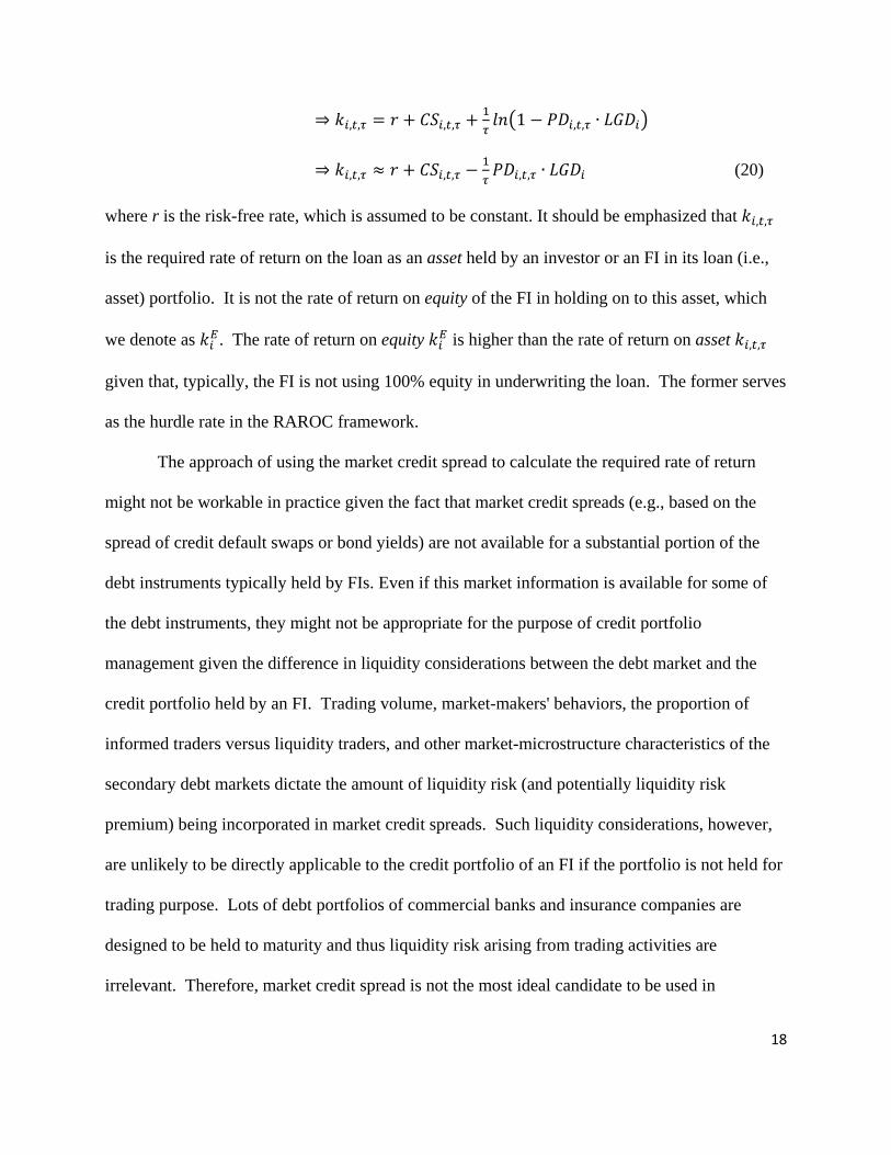
⇒ 𝑘𝑘𝑖𝑖,𝐸𝐸,𝜏𝜏 = 𝑃𝑃 + 𝐸𝐸𝐶𝐶𝑖𝑖,𝐸𝐸,𝜏𝜏 + 1𝜏𝜏𝑙𝑙𝑖𝑖�1 − 𝑃𝑃𝑃𝑃𝑖𝑖,𝐸𝐸,𝜏𝜏 ∙ 𝐿𝐿𝐿𝐿𝑃𝑃𝑖𝑖�

⇒ 𝑘𝑘𝑖𝑖,𝐸𝐸,𝜏𝜏 ≈ 𝑃𝑃 + 𝐸𝐸𝐶𝐶𝑖𝑖,𝐸𝐸,𝜏𝜏 −1𝜏𝜏𝑃𝑃𝑃𝑃𝑖𝑖,𝐸𝐸,𝜏𝜏 ∙ 𝐿𝐿𝐿𝐿𝑃𝑃𝑖𝑖 (20)

where r is the risk-free rate, which is assumed to be constant. It should be emphasized that 𝑘𝑘𝑖𝑖,𝐸𝐸,𝜏𝜏

is the required rate of return on the loan as an asset held by an investor or an FI in its loan (i.e.,

asset) portfolio. It is not the rate of return on equity of the FI in holding on to this asset, which

we denote as 𝑘𝑘𝑖𝑖𝐸𝐸. The rate of return on equity 𝑘𝑘𝑖𝑖𝐸𝐸 is higher than the rate of return on asset 𝑘𝑘𝑖𝑖,𝐸𝐸,𝜏𝜏

given that, typically, the FI is not using 100% equity in underwriting the loan. The former serves

as the hurdle rate in the RAROC framework.

The approach of using the market credit spread to calculate the required rate of return

might not be workable in practice given the fact that market credit spreads (e.g., based on the

spread of credit default swaps or bond yields) are not available for a substantial portion of the

debt instruments typically held by FIs. Even if this market information is available for some of

the debt instruments, they might not be appropriate for the purpose of credit portfolio

management given the difference in liquidity considerations between the debt market and the

credit portfolio held by an FI. Trading volume, market-makers' behaviors, the proportion of

informed traders versus liquidity traders, and other market-microstructure characteristics of the

secondary debt markets dictate the amount of liquidity risk (and potentially liquidity risk

premium) being incorporated in market credit spreads. Such liquidity considerations, however,

are unlikely to be directly applicable to the credit portfolio of an FI if the portfolio is not held for

trading purpose. Lots of debt portfolios of commercial banks and insurance companies are

designed to be held to maturity and thus liquidity risk arising from trading activities are

irrelevant. Therefore, market credit spread is not the most ideal candidate to be used in

19

calculating hurdle rate for the management of these portfolios. In the following section, we

propose a methodology of calculating the required rate of return of debt instruments based on

pure credit risk consideration and thus will not be contaminated by any liquidity risks.

3. Proposed instrument-specific required rate of return and hurdle rate based on Merton's model

We propose an approach to calculate the required rate of return based on Merton's (1974)

credit risk model. Consider a defaultable zero-coupon debt i maturing at time τ from today.

Under risk-neutral valuation, it can be shown that its credit spread can be expressed as:

𝐸𝐸𝐶𝐶𝑖𝑖,𝐸𝐸,𝜏𝜏 = −1𝜏𝜏𝑙𝑙𝑖𝑖�1 − 𝑃𝑃𝑃𝑃𝑖𝑖,𝐸𝐸,𝜏𝜏

𝑄𝑄 ∙ 𝐿𝐿𝐿𝐿𝑃𝑃𝑖𝑖� ≈1𝜏𝜏𝑃𝑃𝑃𝑃𝑖𝑖,𝐸𝐸,𝜏𝜏

𝑄𝑄 ∙ 𝐿𝐿𝐿𝐿𝑃𝑃𝑖𝑖 (21)

where 𝑃𝑃𝑃𝑃𝑖𝑖,𝐸𝐸,𝜏𝜏𝑄𝑄 is the cumulative risk-neutral probability of default (i.e., under the Q-measure) over

risk horizon τ. Note that 𝑃𝑃𝑃𝑃𝑖𝑖,𝐸𝐸,𝜏𝜏𝑄𝑄 is different from 𝑃𝑃𝑃𝑃𝑖𝑖,𝐸𝐸,𝜏𝜏 in Equation (20). The latter is the

physical (i.e., real life) probability of default under the P-measure.

Based on the assumptions of Merton's (1974) model, it can be shown that:

𝑃𝑃𝑃𝑃𝑖𝑖,𝐸𝐸,𝜏𝜏𝑄𝑄 = Φ�Φ−1�𝑃𝑃𝑃𝑃𝑖𝑖,𝐸𝐸,𝜏𝜏� + 𝜇𝜇𝑖𝑖−𝑟𝑟

𝜎𝜎𝑖𝑖√τ� (22)

where Φ(∎) is the cumulative standard normal distribution function; and 𝜇𝜇𝑖𝑖 and 𝜎𝜎𝑖𝑖 are

respectively the expected return and standard deviation of the asset value of the debt issuer.

Based on the capital asset pricing model (CAPM), we have:

𝜇𝜇𝑖𝑖 − 𝑃𝑃 = 𝛽𝛽𝑖𝑖𝑅𝑅(𝑅𝑅𝑚𝑚 − 𝑃𝑃) (23)

where 𝑅𝑅𝑚𝑚 is the expected market return and 𝛽𝛽𝑖𝑖𝑅𝑅 is the beta of the asset return of debt issuer i with

respect to the market. By invoking CAPM and substituting Equation (23) into Equation (22) and

in turn into Equation (21), we have:

20

𝐸𝐸𝐶𝐶𝑖𝑖,𝐸𝐸,𝜏𝜏 = −1𝜏𝜏𝑙𝑙𝑖𝑖 �1 −Φ �Φ−1�𝑃𝑃𝑃𝑃𝑖𝑖,𝐸𝐸,𝜏𝜏� + 𝛽𝛽𝑖𝑖𝑅𝑅

𝑅𝑅𝑚𝑚−𝑟𝑟𝜎𝜎𝑖𝑖

√τ� ∙ 𝐿𝐿𝐿𝐿𝑃𝑃𝑖𝑖� (24)

Based on this model-implied credit spread (of Equation (24)), we can then compute the model-

implied required rate of return 𝑘𝑘𝑖𝑖,𝐸𝐸,𝜏𝜏 according to Equation (20). That is,

𝑘𝑘𝑖𝑖,𝐸𝐸,𝜏𝜏 = 𝑃𝑃 −1𝜏𝜏𝑙𝑙𝑖𝑖 �1 −Φ�Φ−1�𝑃𝑃𝑃𝑃𝑖𝑖,𝐸𝐸,𝜏𝜏� + 𝛽𝛽𝑖𝑖𝑅𝑅

𝑅𝑅𝑚𝑚 − 𝑃𝑃𝜎𝜎𝑖𝑖

√τ� ∙ 𝐿𝐿𝐿𝐿𝑃𝑃𝑖𝑖� +1𝜏𝜏𝑙𝑙𝑖𝑖�1 − 𝑃𝑃𝑃𝑃𝑖𝑖,𝐸𝐸,𝜏𝜏 ∙ 𝐿𝐿𝐿𝐿𝑃𝑃𝑖𝑖�

≈ 𝑃𝑃 +1𝜏𝜏�Φ �Φ−1�𝑃𝑃𝑃𝑃𝑖𝑖,𝐸𝐸,𝜏𝜏� + 𝛽𝛽𝑖𝑖𝑅𝑅

𝑅𝑅𝑚𝑚 − 𝑃𝑃𝜎𝜎𝑖𝑖

√τ�� ∙ 𝐿𝐿𝐿𝐿𝑃𝑃𝑖𝑖 −1𝜏𝜏𝑃𝑃𝑃𝑃𝑖𝑖,𝐸𝐸,𝜏𝜏 ∙ 𝐿𝐿𝐿𝐿𝑃𝑃𝑖𝑖

= 𝑃𝑃 + 1𝜏𝜏�Φ �Φ−1�𝑃𝑃𝑃𝑃𝑖𝑖,𝐸𝐸,𝜏𝜏� + 𝛽𝛽𝑖𝑖𝑅𝑅

𝑅𝑅𝑚𝑚−𝑟𝑟𝜎𝜎𝑖𝑖

√τ� − 𝑃𝑃𝑃𝑃𝑖𝑖,𝐸𝐸,𝜏𝜏� ∙ 𝐿𝐿𝐿𝐿𝑃𝑃𝑖𝑖 (25)

Note that 𝑘𝑘𝑖𝑖,𝐸𝐸,𝜏𝜏 is the required rate of return for holding on to debt instrument i until maturity

date, which is 𝜏𝜏 periods from today. It is the required rate of return on the instrument as an asset

held by the FI in its portfolio. It is not the required rate of return on the equity of the FI in

holding on to this asset, which we denote as 𝑘𝑘𝑖𝑖,𝐸𝐸,𝜏𝜏𝐸𝐸 . The former (𝑘𝑘𝑖𝑖,𝐸𝐸,𝜏𝜏) is the return on asset

measure of the FI, while the latter (𝑘𝑘𝑖𝑖,𝐸𝐸,𝜏𝜏𝐸𝐸 ) is the return on equity measure. The return on equity

measure is higher than the return on asset measure given that the exposure is not 100% equity

financed. In practice, most FIs are heavily leveraged. The allocated capital of any debt

instrument in the portfolio – representing shareholders’ equity – accounts for only a (small)

fraction of the credit exposure; the rest of which is financed by debt (or/and deposits) issued by

the FI. To find out the required rate of return of the FI's shareholders, we therefore need to

account for the additional return the shareholders would require given the higher risk that they

are assuming as a result of this financial leverage. Thus, it is 𝑘𝑘𝑖𝑖,𝐸𝐸,𝜏𝜏𝐸𝐸 rather than 𝑘𝑘𝑖𝑖,𝐸𝐸,𝜏𝜏 that serves as

the instrument's RAROC hurdle rate.

To conduct the transformation from return on asset to return on equity, we apply the

Modigliani-Miller Theorem based on the allocated economic capital of each instrument:

21

𝑘𝑘𝑖𝑖𝐸𝐸 = 𝑘𝑘𝑖𝑖 + �Exposure𝑖𝑖−𝐶𝐶𝑖𝑖�𝐶𝐶𝑖𝑖

∙ (𝑘𝑘𝑖𝑖 − 𝑘𝑘𝐵𝐵) (26)

where 𝐸𝐸𝑖𝑖 is the allocated economic capital, �Exposure𝑖𝑖 − 𝐸𝐸𝑖𝑖� is the remaining portion of the

credit exposure that is financed by debt issued by the FI, and 𝑘𝑘𝐵𝐵 represents the FI's cost of debt.

Without loss of generality, we suppress subscripts t and 𝜏𝜏 in Equation (26).

It is worthwhile to note that one of the possible obstacles in the implementation of this

methodology is the potential lack of market information to calculate the beta (𝛽𝛽𝑖𝑖𝑅𝑅) for the asset

return of each obligor in the FI’s credit portfolio. For a lot of FIs, many of the debt contracts

within their credit portfolios are written to non-publicly traded obligors for which equity and

debt data will not be available in estimating asset betas. Nevertheless, for FIs that utilize

multifactor models to calculate capital requirements for their credit portfolios, the correlation

assumptions between asset returns and market-wide returns required to calculate asset beta are

already being made within the economic capital calculation framework itself. By adopting these

assumptions consistently in the calculation of asset beta and in turn the hurdle rate via Equations

(25) and (26), our proposed methodology is readily applicable even to credit portfolios consisting

predominantly of non-publicly traded obligors. To calculate the proposed hurdle rate, an FI,

currently utilizing a multifactor model in computing its economic capital, should not require any

additional information other than that which has already been used in its economic capital

framework.5

5 For example, in Moody’s KMV RiskFrontier®, which uses the proprietary GCorr® factor model, individual instruments are assigned sector and geographic classifications which together with the instrument’s R-squared value are then used to generate correlated asset returns in the simulation of the one-year distribution of portfolio loss. The resulting weighting of the instrument’s underlying asset return on the global factor within GCorr® implies a covariance between asset returns and market returns, which can be used to calculate the beta of the instrument’s underlying asset.

22

4. Demonstration of the proposed methodology

We operationalize the proposed methodology by conducting a RAROC performance

measurement exercise with a real-life credit portfolio using tools and information that are readily

available to most financial institutions. We demonstrate how we may conduct capital allocation

and arrive at risk-adjusted performance measurements incorporating both the shareholders' and

debt-holders' perspective. Three steps are involved in achieving this objective. In the first step

(see Section 4.1), we compute the overall economic capital 𝐸𝐸𝐸𝐸𝑝𝑝 of our portfolio satisfying the

risk appetite of the FI's debtholders by making sure that the expected shortfall conforms with the

confidence level implicit in its target credit rating. We then allocate this required capital to

individual debt instruments using the tail risk allocation methodology. In the second step (see

Section 4.2), we compute the required rate of return of each debt instrument in our portfolio

following the approach outlined in Section 3. In the last step (see Section 4.3), using the

allocated capital from the first step and the required rate of return from the second step, we

conduct performance measurements by calculating the required dollar amount net return for each

debt instrument. Only if the instruments can generate these required returns can we ensure the

FI's shareholders are sufficiently compensated on a risk-adjusted basis. Finally, using indicative

market credit spreads, we demonstrate the importance of using instrument-specific hurdle rates

in comparing risk-adjusted performances of a subset of the debt instruments in our portfolio.

Before we go through the three steps of our RAROC exercise, let us first briefly describe

how we construct our credit portfolio to be used in the rest of this study. Our objective is to

come up with a portfolio that resembles a plausible credit portfolio that is held by a large

commercial bank operating in North America. We start with the largest 1,000 North American

23

public firms by asset values obtained from Compustat as of the end of July 2011. To ensure that

we are focusing on firms that are likely to be issuing debts and/or borrowing from banks, we

exclude from our sample firms with low debt levels. We also exclude firms with insufficient

debt history and incomplete equity return information during the 12 months prior to the end of

July 2011. Our final sample includes 785 large publicly-traded firms operating in 38 different

industry sectors (see Appendix A, Table A1). We therefore arrive at a sample of potentially the

largest corporate debtors from a diverse industry background, which are likely to borrow from

commercial banks with different forms of debt instruments (e.g., term loans, corporate bonds).

As of the end of July 2011, we construct a hypothetical, though realistic, credit portfolio

for an FI, which underwrites debt instruments to this sample of 785 obligors. In determining the

exposure to each of these obligors, we respect the concentration limits typically enforced by an

FI. Specifically, the amount of exposure to each obligor is determined based on a three-step

process. First, the exposure was set proportional to the total value of the firm’s debt outstanding

as of end of July 2011 (obtained from Compustat). Next, sectoral maximum exposure limits

were applied to each industry sector to ensure that no single industry made up of more than 7%

of the overall exposure of the portfolio. Finally, a single-name concentration limit is applied to

ensure that no single entity made up of more than 1% of the total exposure of the portfolio.

Based on this three-step process, the largest exposure obligors, as expected, are primarily

financial institutions followed by firms in the Oil & Gas and the Utilities sectors (see Appendix

A Table A2 for a breakdown of portfolio exposure by industry sectors and Table A3 for the top

30 obligors by exposure). The portfolio exposure is predominantly on firms incorporating in the

United States (87%, by exposure), although there are exposures on obligors from ten other

countries, including Canada (9%), Bermuda (2%), Switzerland (1%), and the Cayman Islands

24

(0.25%). All of the firms are listed on the stock exchanges of the United States or Canada with

assets primarily in North America. In Table 1, we present the summary statistics of the equity

values, total asset values, and values of debt outstanding of the 785 firms in our sample.

Consistent with the credit risk modeling practice (e.g., the distance-to-default model of Moody's

KMV), we present the summary statistics for the full short-term debt plus half long-term debt. In

Table 2, we report the exposure and obligor count distribution by credit rating agency grades as

of end of July 2011. The portfolio we have constructed is considered to be well-diversified. It is

made up of obligors of relatively large firms and of both investment and non-investment grade.6

The portfolio has an overall exposure of $14,778 million on debts issued by the 785 obligors.

INSERT TABLES 1 AND 2 HERE

4.1. Portfolio economic capital and tail-risk capital allocation

We use a proprietary credit portfolio simulation engine adopted by a bank to calculate the

expected shortfall (see Equation (15)) of the portfolio over a one-year risk horizon. The

proprietary simulation engine operates in a similar fashion as Moody’s KMV RiskFrontier®,

which simulates the portfolio loss distribution using Monte Carlo simulation and recognizes the

correlation of asset value returns of the obligors within the portfolio (see Moody’s KMV

Company, 2007). We adopt a confidence level (δ) of 99.96%, which is considered to be

consistent with a target debt rating of A (Jackson et al., 2002). We use the following information

specific to each debt instrument of our portfolio:

6 Quite a number of the obligors in our portfolio have relatively low credit rating (e.g., B or below). Although it is quite unlikely that a typical FI will enter into a loan agreement with an obligor of such a low credit rating, we may indeed find lowly-rated obligors in existing credit portfolio of an FI as the financial health of some of the originally credit-worthy obligors has deteriorated due to firm-specific and/or market-wide conditions.

25

o Probability of default (PD): We use Moody's KMV's one-year expected default frequency

(EDF) of the obligors (as of the end of July 2011) to proxy for their one-year probabilities

of default;

o Loss-given-default (LGD): Without loss of generality, we assume an LGD of 50% for all

instruments. A 50% LGD is similar to that documented in the empirical research on the

recovery rates of bank loans (e.g., Keisman and Marshella, 2009);

o Exposure-at-default (EAD): We assume all instruments are fully drawn and thus EAD is

100%;

o Exposure of instrument: We use the exposure obtained earlier in this section in

constructing our representative portfolio;

o Maturity of contract: We assume a uniform time-to-maturity of one year;

o Cash flow: We assume the instruments are zero-coupon instruments with the payoff of

the face value at maturity and no intermediate cash flows;

o Asset return correlation (usually referred to as "R-square"): We use the "R-square"

obtained from Moody's KMV's GCorr® model for each obligor as of end of July 2011.

The "R-square" measures the correlation of the return on assets of obligors based on a

factor model making up of global, regional, and industrial factors (Levy, 2008).

In Table 3, we present the summary statistics of the key input parameters. With the

above inputs, the expected shortfall of our portfolio is estimated to be $1,019 million by using

the proprietary simulation engine and based on the 99.96% confidence level.

INSERT TABLE 3 HERE

Capital allocation is performed using again the proprietary simulation engine while

adopting the tail risk allocation methodology of Equation (18) with 𝛿𝛿1 set at 99.96%. The largest

26

30 obligors by the amount of allocated capital are presented in Table 4 together with their PDs,

R-squares, industry sectors, and exposures. In the tail risk allocation approach, capital is

allocated based on the contribution to the loss tail, which is primarily driven by the obligors' PDs

and R-squares. Not surprisingly, a number of the top thirty obligors (e.g., Nelnet Inc.,

Community Health Systems Inc., etc) have relatively high PD compared to the average. A

majority of the other top obligors have high R-square (e.g., Goldman Sachs Group Inc.,

Prudential Financial Inc., Metlife Inc., etc). Moreover, as expected, obligors with larger

exposures (e.g., Goldman Sachs Group Inc.) are allocated more capital. A total of 18 out of the

top 30 obligors are FIs. But there are also obligors from a variety of industry sectors. In Table

5, we show the breakdown of both allocated capital and exposure by industry sectors.

Altogether, FIs contribute to 42% of the overall portfolio EC. Oil & Gas, Utilities, and Business

Service sectors are also well represented, contributing to respectively 9.1%, 10.1%, and 4.9% of

the overall EC.

INSERT TABLES 4 AND 5 HERE

4.2. Computation of required rate of return

We compute the required rate of return 𝑘𝑘𝑖𝑖,𝐸𝐸,𝜏𝜏 for each debt instrument in our portfolio by

using Equation (25). We use the same obligor- and instrument-specific information, namely,

PD, LGD, EAD, time-to-maturity, cash flow, and asset return correlation, as used in Section 4.1

in calculating the allocated capital. We obtain the ratio of beta of the asset return and standard

deviation of the asset return of each obligor (i.e., 𝛽𝛽𝑖𝑖𝑅𝑅 𝜎𝜎𝑖𝑖⁄ ) from Moody's KMV's GCorr® (see

27

Levy, 2008) as of the end of July 2011.7 We assume a market risk premium of (𝑅𝑅𝑚𝑚 − 𝑃𝑃) of 6%,

which is considered to be consistent with the findings from the analysis on market-implied equity

risk premium (e.g., Damodaran, 2012). We also assume a risk-free interest rate (𝑃𝑃) of 2%.

In Table 6, we report the summary statistics of the estimated required rates of return for

all obligors (Row 1) and for obligors of different industry sectors. The overall mean (median) of

the required rates of return is 2.35% (2.19%).

INSERT TABLE 6 HERE

From Table 6, we observe that obligors from different industries could have very

different required rate of returns. In particular, Financial, Oil & Gas, Telecom, and Metal

Products sectors tend to have higher than average required rate of return reflecting the higher

systematic risks for these sectors. Nevertheless, based on the standard deviations reported in

Table 6, there is significant cross-sectional variation of the required rate of return within each

industry sector. It therefore suggests that the required rate of return is not solely determined by

the industry effect.

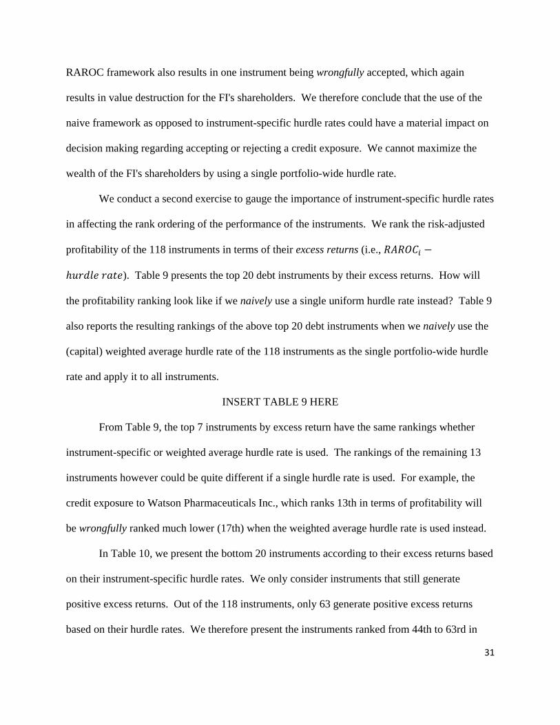
Table 7 presents the statistics of the estimated required rate of return by the obligor's

S&P's credit rating. We also plot the mean value of the estimated required rate of return against

credit rating in Figure 1 (which also shows the total amount of exposure in each credit grade). It

seems that the credit worthiness of the obligor is a key driver of its required rate of return. In

general, the lower the credit rating of the obligor, the higher is its required rate of return. This

credit rating effect is considered to be economically significant. For example, the required rates

of return for B rated obligors are on average more than 100 basis points higher than those of AA

7 Note that the GCorr model is a multifactor model. As a result, one may argue that the asset beta derived from the GCorr model may not be the same as the asset beta of the CAPM model. For those publicly-traded obligors with valid market information, rather than using the GCorr model, one may conduct her own estimations of beta and standard deviation of asset return of each obligor by adopting a market model.

28

rated ones. Comparing Table 6 and 7, it seems that the credit rating effect dominates the industry

effect in dictating an obligor's required rate of return. Nevertheless, there is still a significant

variation of required rates of return across obligors within each credit rating, as manifested in the

standard deviations reported in Table 7. This intra-rating variation tends to be higher for lower

credit ratings.

INSERT TABLE 7 AND FIGURE 1 HERE

We conduct a number of sensitivity analyses (results not reported) to gauge the impact of

some of the key input parameters on our results. Specifically, we re-run the above analysis using

different terms to maturity, risk-free rates, LGDs, and different target debt ratings for the FI. Our

key findings and conclusions remain robust. For example, increasing the LGD from 50% to

75% results in an increase in the required rates of return for all the instruments. Nevertheless,

we still observe the same cross-sectional patterns among different industry sectors and credit

ratings as documented in Tables 6 and 7; albeit the cross-sectional differences become more

salient. The results of these sensitivity analyses are available from the authors.

4.3. Hurdle rate and RAROC

Using the allocated capital obtained in Section 4.1 together with the instrument-specific

required rate of return from Section 4.2, we can assess the risk-adjusted performance by

calculating the minimum required dollar amount of expected income for each debt instrument in

the portfolio. The minimum required expected income from instrument 𝑖𝑖 is simply the sum of

the required dollar amount return for shareholders (i.e., 𝐸𝐸𝑖𝑖 ∙ 𝑘𝑘𝑖𝑖𝐸𝐸 ) and the financing cost of the

instrument (i.e., �Exposure𝑖𝑖 − 𝐸𝐸𝑖𝑖� ∙ 𝑘𝑘𝐵𝐵). Only if the instrument is expected to generate this

income can we ensure the FI's shareholders are sufficiently compensated on a risk-adjusted basis.

29

We consider a hypothetical FI having the credit portfolio of the 785 debt instruments

constructed above as its only assets. Based on the allocated capital calculated in Section 4.1, we

compute the RAROC hurdle rate using Equation (26) and then the corresponding minimum

required dollar amount of expected income for each of the 785 debt instruments. We report the

results for the top 20 obligors by allocated capital in Table 8.8 The weighted average RAROC

hurdle rate (weighted by allocated capital) across all the debt instruments is 8.28%.

INSERT TABLE 8 HERE

To demonstrate the economic significance of using our proposed instrument-specific

hurdle rates as opposed to the common practice of using a single portfolio-wide hurdle rate in

performance measurement, we conduct an exercise to examine the implications on the decision

of accepting/rejecting a debt instrument. We consider 118 debt instruments in our portfolio for

which we observe valid one-year CDS spreads (from Bloomberg) as of end of July 2011. Using

these market CDS spreads (𝐸𝐸𝐶𝐶𝑖𝑖𝑀𝑀𝐵𝐵𝑟𝑟𝐵𝐵𝐸𝐸𝐸𝐸) to proxy for the one-year credit spreads of these debt

instruments, we calculate their RAROC by:9

𝑅𝑅𝑅𝑅𝑅𝑅𝑅𝑅𝐸𝐸𝑖𝑖 = 𝐸𝐸𝐸𝐸𝑝𝑝𝐸𝐸𝐸𝐸𝐸𝐸𝐸𝐸𝐸𝐸 𝑅𝑅𝐸𝐸𝑅𝑅𝐸𝐸𝑛𝑛𝑅𝑅𝐸𝐸𝑅𝑅𝑖𝑖 - 𝐶𝐶𝐶𝐶𝑅𝑅𝐸𝐸𝑅𝑅i - 𝐸𝐸𝐸𝐸𝑝𝑝𝐸𝐸𝐸𝐸𝐸𝐸𝐸𝐸𝐸𝐸 𝐿𝐿𝐶𝐶𝑅𝑅𝑅𝑅𝐸𝐸𝑅𝑅𝑖𝑖𝐶𝐶𝑖𝑖

=Exposurei∙�𝑟𝑟𝑓𝑓+𝐶𝐶𝑆𝑆𝑖𝑖

𝑀𝑀𝐵𝐵𝑀𝑀𝑘𝑘𝑀𝑀𝑡𝑡� - �Exposure𝑖𝑖−𝐶𝐶𝑖𝑖�∙𝐵𝐵𝐵𝐵 - Exposure𝑖𝑖∙�1+𝑟𝑟𝑓𝑓+𝐶𝐶𝑆𝑆𝑖𝑖

𝑀𝑀𝐵𝐵𝑀𝑀𝑘𝑘𝑀𝑀𝑡𝑡�∙𝑆𝑆𝑃𝑃𝑖𝑖∙𝐿𝐿𝐿𝐿𝑃𝑃𝑖𝑖𝐶𝐶𝑖𝑖

(27)

8 In evaluating Equation (26), we further assume the cost of debt of the FI (𝑘𝑘𝐵𝐵) equals to the risk-free interest rate of 2%. Although short-term funding for an FI is likely to be much more expensive than the risk-free interest rate, the weighted average cost of debt of deposit-taking FIs could be lower and not very different from the risk-free rate given the substantial size of their low-cost deposit bases. 9 As discussed earlier in the paper, the observed market CDS spreads account for more than just the credit risk of the debt instruments, as they may contain a significant liquidity premium. Therefore, the expected income implied by the CDS spread is likely to be higher than the true expected income that is solely based on the credit risk of the obligor. As a result, we will tend to overstate the number of instruments having RAROCs that exceed their respective hurdle rates. When implementing the proposed methodology in practice, a financial institution should have all the actual income information of each instrument in its credit portfolio to calculate the RAROC measures.

30

In calculating RAROC, we assume 𝑘𝑘𝐵𝐵 = 𝑃𝑃𝑓𝑓 = 2%, 𝑃𝑃𝑃𝑃𝑖𝑖 equals to the one-year KMV's

EDF of the obligor, and 𝐿𝐿𝐿𝐿𝑃𝑃𝑖𝑖 = 50%. If the resulting RAROC of a debt instrument is higher

(lower) than the corresponding instrument-specific hurdle rate from Equation (26), the

instrument is deemed creating (destroying) shareholders' values and thus should be accepted

(rejected). Based on this acceptance/rejection criteria, 55 (63) out of the 118 loans will be

rejected (accepted) because their RAROCs are lower (higher) than the corresponding instrument-

specific hurdle rates.10

How will the results be different if we ignore instrument-specific hurdle rates and, like

many commonly-used RAROC frameworks, naively use a single uniform hurdle rate as the

benchmark in comparing with the RAROC of all the debt instruments? We repeat the above

acceptance/rejection checks but now using the weighted average (by allocated capital) hurdle

rate of 7.53% of our sub-portfolio of 118 debt instruments as the single uniform hurdle rate for

all the debt instruments. Comparing with the acceptance/rejection results documented

previously, this naive RAROC framework results in eight instruments being wrongfully rejected.

These eight debt instruments actually contribute positively to shareholders' wealth given the fact

that they can generate amounts of expected incomes that exceed the minimum requirements

according to their instrument-specific hurdle rates. They are nevertheless rejected in the naive

RAROC framework when a single portfolio-wide hurdle rate is applied. The use of the naive

10 An important limitation of RAROC analysis is highlighted in the comparison of the relative performance of instruments. That is, the RAROC of any individual instrument is dependent on the legacy portfolio to which it has been added. For example, a new loan underwritten to an information technology company will attract a higher capital requirement if the existing loan portfolio already has a high concentration on information technology obligors than if the existing portfolio is in fact well diversified. Thus, the RAROC of a new loan and, in turn, whether it will create value for the shareholders of the FI are dictated by the composition of the existing portfolio. Moreover, as removing loans from a portfolio affects the capital requirements of the remaining loans, the results of portfolio management on a RAROC basis can vary depending on the order in which underperforming loans are removed. This is a noteworthy shortcoming of RAROC metrics that deserves further study and investigation. In the present study, we focus on how we may improve the RAROC analysis by introducing differentiated and instrument-specific hurdle rates.

31

RAROC framework also results in one instrument being wrongfully accepted, which again

results in value destruction for the FI's shareholders. We therefore conclude that the use of the

naive framework as opposed to instrument-specific hurdle rates could have a material impact on

decision making regarding accepting or rejecting a credit exposure. We cannot maximize the

wealth of the FI's shareholders by using a single portfolio-wide hurdle rate.

We conduct a second exercise to gauge the importance of instrument-specific hurdle rates

in affecting the rank ordering of the performance of the instruments. We rank the risk-adjusted

profitability of the 118 instruments in terms of their excess returns (i.e., 𝑅𝑅𝑅𝑅𝑅𝑅𝑅𝑅𝐸𝐸𝑖𝑖 −

ℎ𝐴𝐴𝑃𝑃𝐴𝐴𝑙𝑙𝐴𝐴 𝑃𝑃𝑉𝑉𝐴𝐴𝐴𝐴). Table 9 presents the top 20 debt instruments by their excess returns. How will

the profitability ranking look like if we naively use a single uniform hurdle rate instead? Table 9

also reports the resulting rankings of the above top 20 debt instruments when we naively use the

(capital) weighted average hurdle rate of the 118 instruments as the single portfolio-wide hurdle

rate and apply it to all instruments.

INSERT TABLE 9 HERE

From Table 9, the top 7 instruments by excess return have the same rankings whether

instrument-specific or weighted average hurdle rate is used. The rankings of the remaining 13

instruments however could be quite different if a single hurdle rate is used. For example, the

credit exposure to Watson Pharmaceuticals Inc., which ranks 13th in terms of profitability will

be wrongfully ranked much lower (17th) when the weighted average hurdle rate is used instead.

In Table 10, we present the bottom 20 instruments according to their excess returns based

on their instrument-specific hurdle rates. We only consider instruments that still generate

positive excess returns. Out of the 118 instruments, only 63 generate positive excess returns

based on their hurdle rates. We therefore present the instruments ranked from 44th to 63rd in

32

Table 10. We also present in Table 10 the resulting rankings when the weighted average hurdle

rate is used as the single portfolio-wide hurdle rate that is applied to all the instruments.

Comparing with Table 9, Table 10 provides an even stronger illustration of the implications of

applying a single portfolio-wide hurdle rate to those instruments that are close to break even in

terms of their profitability. We will not be able to rank them accurately if we apply a single

uniform hurdle rate. In fact, eight of these 20 instruments will be wrongfully rejected when the

uniform hurdle rate is used given their negative excess returns.

We also conduct a number of sensitivity analyses by using different terms to maturity,

risk-free rates, LGDs, and different target debt ratings for the FI. Our key findings and

conclusions remain robust. The degree of distortion to the profitability rankings when the single

uniform hurdle rate is used instead of the instrument-specific ones is essentially unaffected by

these alternative assumptions. The results of these sensitivity analyses are available from the

authors.

INSERT TABLE 10 HERE

In Figure 2, we plot the profitability ranking of each of the instruments based on the

naive approach of using the weighted average hurdle rate (vertical axis) against those from using

instrument-specific hurdle rate (horizontal axis). The smaller the ranking number, the higher is

its profitability in terms of excess return. Those observations above (below) the 45-degree line

indicates that applying the uniform hurdle rate in assessing performance understates (overstates)

profitability. We observe from Figure 2 that there are quite a number of instruments within the

middle range of profitability of which their rankings are either significantly overstated or

understated if we ignore the cross-sectional difference in their hurdle rates and naively apply a

uniform hurdle rate.

33

INSERT FIGURE 2 HERE

In practice, the uniform hurdle rate applied to the debt instruments of a credit portfolio

held by an FI is generally derived with a more subjective approach that may be completely

unrelated to even the average characteristic of the portfolio. The findings of the above exercise

therefore likely understate the errors resulting from the common practice of using a single

institution-wide hurdle rate in assessing profitability. At least, in our naive approach, we use the

portfolio weighted average hurdle rate that corresponds to an average instrument within the

portfolio. That is, there is still a connection between the characteristics of the portfolio and the

uniform hurdle rate being applied. But even that, as demonstrated above, the resulting errors in

deciding on accepting/rejecting a credit exposure and in profitability ranking could be more

significant than one would want to ignore. Ignoring instrument-specific hurdle rate in the

RAROC framework could jeopardize the ability of an FI to achieve its objective of maximizing

its shareholders' wealth.

5. Conclusion

Based on the structural credit risk model of Merton (1974), we propose a methodology to

estimate instrument-specific expected rate of return that can serve as hurdle rate in RAROC

performance assessment and dynamic credit portfolio management. By being able to

differentiate the systematic risks inherent in debt instruments issued by different obligors, the

proposed methodology allows us to more accurately measure the risk-adjusted profitability of the

instruments than the RAROC framework typically adopted in practice, where a single uniform

portfolio-wide hurdle rate is applied to all the debt instruments. When using the proposed hurdle

34

rates together with the economic capital allocated using the tail risk allocation methodology, we

establish a RAROC framework that incorporates the risk concerns of both the debtholders and

shareholders of financial institutions.

We implement our proposed methodology of calculating instrument-specific hurdle rates

on a representative credit portfolio. With obligor-specific information, we demonstrate how we

can estimate the hurdle rate for each of the debt instruments in our portfolio. We then show that

the decision of accepting/rejecting a credit exposure could be significantly distorted if we ignore

the instrument-specific hurdle rate and apply a single uniform hurdle rate to all the instruments.

In particular, among the debt instruments under consideration, some that are deemed to create

shareholders' value will be wrongfully rejected if the uniform hurdle rate were used as the

acceptance benchmark. Naively using this uniform hurdle rate may also result in a distorted

profitability ranking of instruments and thus forbids us to maximize the wealth of the

shareholders of financial institutions.

35

References: Acerbi, C., and Tasche, D., 2002. Expected shortfall: A natural coherent alternative to value at risk. Economic Notes 31 (2), 379-388. Artzner, P., Delbaen, F., Eber, J.-M., and Heath, D., 1999. Coherent measures of risk. Mathematical Finance 9 (3), 203–228. Baer, T., Mehta, A and Samandari, H., 2011. The use of economic capital in performance management for banks: A perspective. McKinsey & Company. Basel Committee on Banking Supervision (BCBS), 2010. Basel III: International framework for liquidity risk measurement, standards and monitoring. Bank for International Settlements. Crouhy, M., Galai, D., and Mark, R., 2006. The Essentials of Risk Management. McGraw Hill Companies, Inc. Crouhy, M., Turnbull, S.M., and Wakeman, L.M., 1999. Measuring risk-adjusted performance. Journal of Risk 2 (1), 5-35. Damodaran, A., 2012. Equity Risk Premiums (ERP): Determinants, Estimation and Implications – the 2012 edition. Working paper, Stern School of Business, http://papers.ssrn.com/sol3/papers.cfm?abstract_id=2027211 Dhaene, J., Tsanakas, A., Valdez, E., and Vanduffel, S., 2009. Optimal Capital Allocation Principles. The 9th International Congress on Insurance: Mathematics and Economics (MIE2005). Drzik, J., Nakada, P., and Schuermann, T., 1998. The debtholder's perspective: risk, capital, and value measurement in financial institutions - part I. The Journal of Lending & Credit Risk Management, September 1998. Froot, K.A., and Stein, J.C., 1998. Risk management, capital budgeting, and capital structure policy for financial institutions: an integrated approach. Journal of Financial Economics 47, 55-82. Jackson, P., Perraudin, W., and Sapporta, V., 2002. Regulatory and “economic” solvency standards for internationally active banks. Journal of Banking and Finance 26, 953–976.

36

James, C., 1996. RAROC based capital budgeting and performance evaluation: a case study of bank capital allocation. The Wharton Financial Institutions Center working paper 96-40. James, C., and Kizilaslan, A., 2010. Asset specificity, industry driven recovery risk and loan pricing. Forthcoming in the Journal of Financial and Quantitative Analysis. Kalkbrener, M., 2005. An axiomatic approach to capital allocation. Mathematical Finance 15, 425-437. Kalkbrener, M., Lotter, H., and Overbeck, L., 2004. Sensible and efficient capital allocation for credit portfolios. Risk (January), S19–S24. Keisman, D. and Marshella, T., 2009. Recoveries on Defaulted Debt In an Era of Black Swans. Moody’s Global Corporate Finance, Moody’s Investments Service. Kimball, R.C., 1998. Economic Profit and Performance Measurement in Banking. New England Economic Review, July/August 1998, 35-53. Levy, A., 2008. An Overview of Modeling Credit Portfolios. Moody’s KMV Company. Merton, R.C., 1974. On the pricing of corporate debt: The risk structure of interest rates. Journal of Finance 29, 449-470. Mehta, A., Neukirchen, M., Pfetsch, S., and Poppensieker, T., 2012. Managing Market Risk: Today and Tomorrow. McKinsey Working Papers on Risk, Number 32, McKinsey & Company. Milne, A., and Onorato, M., 2012. Risk-adjusted measures of value creation in financial institutions. European Financial Management 18 (4), 578-601. Moody’s KMV Company, 2007. Why Choose RiskFrontierTM? Rosen, D., and Saunders, D., 2010. Risk factor contributions in portfolio credit risk models. Journal of Banking and Finance 34, 336-349. Stoughton, N.M., and Zechner, J., 2007. Optimal capital allocation using RAROC and EVA. Journal of Financial Intermediation 16, 312–342. Tasche, D., 2008. Capital Allocation to Business Units and Sub-Portfolios: The Euler Principle. In Resti, A. (Ed.), Pillar II in the new Basel Accord: The Challenge of Economic Capital. Risk Books, London, pp.423-453.

37

Vasicek, O., 1987. Probability of loss on loan portfolio. KMV Corporation. Wilson, T., 2003. Overcoming the hurdle. Risk, July 2003, 79-83. Zaik, E., Walter, J., Kelling, G., and James, C., 1996. RAROC at Bank of America: From theory to practice. Journal of Applied Corporate Finance 9 (2), 83-93.

38

Table 1: Summary statistics of equity value, asset value, and debt value of the 785 obligors.

Equity ($M) Asset Value ($M) Full Short-Term Debt plus Half Long-Term Debt ($M)

Median 2,452 3,821 927 Average 7,457 14,535 7,151 Minimum 242 503 1.0 Maximum 183,039 985,136 845,775 Std. Dev. 15,186 54,271 45,584

39

Table 2: Exposure and obligor count distribution by credit rating agency grades (as of end of July 2011)

S&P's Ratings Moody's Ratings Rating Exposure Percent Count Percent Rating Exposure Percent Count Percent AAA 0.4% 0.1% Aaa 0.8% 0.3% AA 3.5% 1.5% Aa 2.0% 0.8% A 14.2% 7.4% A 12.2% 6.4%

BBB 34.4% 25.1% Baa 26.7% 18.6% BB 13.9% 14.7% Ba 10.8% 10.2% B 6.9% 7.5% B 11.1% 11.7%

CCC-C 0.2% 0.5% Caa-C 1.0% 1.4% Unrated 26.5% 43.2% Unrated 35.4% 50.8%

40

Table 3: Summary statistics of key input parameters of the debt instruments.

R-square PD Exposure ($M)

Median 0.228 0.23% 15.2 Average 0.237 0.74% 18.6 Minimum 0.100 0.01% 1.0 Maximum 0.650 35.0% 130.7 Std. Dev. 0.084 1.72% 13.0

41

Table 4: The largest 30 obligors by allocated capital

Identifier Counterparty Name PD R-square Industry Exposure

Capital ES

99.96% Capital

(%) GS GOLDMAN SACHS GROUP INC 0.22% 0.65 Non-Bank FI 130.68 25.26 2.48% BNS BANK OF NOVA SCOTIA 0.42% 0.59 Commercial Bank 99.46 24.93 2.45% TD TORONTO DOMINION BANK 0.25% 0.59 Commercial Bank 99.46 20.28 1.99% PRU PRUDENTIAL FINANCIAL INC 2.59% 0.65 Insurance 38.65 14.13 1.39% WFC WELLS FARGO & CO 0.39% 0.54 Commercial Bank 99.46 14.09 1.38% MET METLIFE INC 2.68% 0.60 Insurance 38.65 13.76 1.35% AFL AFLAC INC 0.88% 0.42 Insurance 74.08 13.36 1.31% NNI NELNET INC 35.00% 0.33 Financial Services 43.25 11.89 1.17% CNO CNO FINANCIAL GROUP INC 2.23% 0.43 Insurance 47.22 11.56 1.13% FFG FBL FINANCIAL GROUP INC-CL A 3.93% 0.44 Insurance 35.05 10.03 0.98% UAL UNITED CONTINENTAL HLDGS INC 2.59% 0.35 Air Transport 52.46 9.85 0.97% EIX EDISON INTERNATIONAL 0.80% 0.55 Utilities 39.74 9.17 0.90% SNV SYNOVUS FINANCIAL CORP 3.28% 0.38 Commercial Bank 41.06 8.86 0.87% NDAQ NASDAQ OMX GROUP INC 5.84% 0.17 Non-Bank FI 41.16 8.43 0.83% AIZ ASSURANT INC 1.76% 0.41 Insurance 43.82 8.39 0.82% CMS CMS ENERGY CORP 1.76% 0.51 Utilities 30.98 8.38 0.82% AXP AMERICAN EXPRESS CO 0.15% 0.49 Financial Services 97.63 8.36 0.82% FE FIRSTENERGY CORP 0.58% 0.53 Utilities 45.45 7.92 0.78% X UNITED STATES STEEL CORP 4.80% 0.32 Metal Products 30.84 7.78 0.76% MFC MANULIFE FINANCIAL CORP 0.54% 0.65 Insurance 38.65 7.59 0.74% S SPRINT NEXTEL CORP 2.44% 0.30 Telecoms 48.54 6.56 0.64% CYH COMMUNITY HEALTH SYSTEMS INC 6.12% 0.22 Medical Services 32.46 6.18 0.61% IVR INVESCO MORTGAGE CAPITAL INC 3.04% 0.11 Funds 36.99 6.17 0.61% ICE INTERCONTINENTALEXCHANGE INC 2.27% 0.14 Non-Bank FI 57.54 6.09 0.60% SHLD SEARS HOLDINGS CORP 1.72% 0.28 Retail & Wholesale 40.86 5.96 0.59% SHAW SHAW GROUP INC 5.02% 0.25 Business Service 27.79 5.86 0.57% AEP AMERICAN ELECTRIC POWER CO 0.27% 0.55 Utilities 45.29 5.79 0.57% ORI OLD REPUBLIC INTL CORP 1.23% 0.39 Insurance 34.09 5.53 0.54% BXS BANCORPSOUTH INC 2.81% 0.39 Commercial Bank 30.31 5.50 0.54% BDN BRANDYWINE REALTY TRUST 2.68% 0.35 Funds 26.04 5.50 0.54%

All Other Exposure 13,230.31 715.99 70.25% Total 14,777.99 1,019.17 100.00%

42

Table 5: Capital allocation by industry sector

Sector Exposure ($ million)

Exposure (%)

Allocated capital ($ million)

Allocated capital (%)

Financial Sector 3,978.24 26.92% 430.97 42.29% Commercial Bank 1,128.00 7.63% 122.71 12.04%

Funds 1,049.20 7.10% 82.14 8.06% Insurance 1,034.69 7.00% 143.16 14.05%

Non-Bank FI 529.75 3.58% 58.69 5.76% Financial Services 236.60 1.60% 24.27 2.38%

Business Service 1,292.12 8.74% 50.29 4.93% Oil & Gas 1,320.50 8.94% 92.41 9.07%

Oil & Gas, Exploration 1,036.79 7.02% 74.25 7.29% Oil & Gas, Refining 283.70 1.92% 18.16 1.78%

Utilities 1,199.50 8.12% 103.21 10.13% Chemicals 811.04 5.49% 24.63 2.42% Retail & Wholesale 747.99 5.06% 32.70 3.21% Consumer Durables 562.10 3.80% 30.57 3.00% Aerospace & Defence 554.66 3.75% 10.62 1.04% Telecoms 479.58 3.25% 30.39 2.98% Automotive 455.56 3.08% 29.44 2.89% Equipment 447.67 3.03% 21.27 2.09% Machinery & Equipment 442.97 3.00% 27.49 2.70% Rail & Water Transportation 314.57 2.13% 21.73 2.13% Food Manufacturing 312.12 2.11% 8.01 0.79% Metal Products 289.95 1.96% 26.48 2.60% Paper Products 180.66 1.22% 6.55 0.64% Medical Services 170.54 1.15% 9.90 0.97% Mining 168.73 1.14% 8.60 0.84% Construction 162.59 1.10% 13.84 1.36% Entertainment 131.48 0.89% 6.11 0.60% Real Estate 119.96 0.81% 5.13 0.50% Hotels & Restaurants 114.16 0.77% 2.95 0.29% Land Transport 96.01 0.65% 2.24 0.22% Air Transport 95.65 0.65% 12.16 1.19% Clothing Manufacturing 87.74 0.59% 2.95 0.29% Consumer Services 64.69 0.44% 3.66 0.36% Agriculture 46.20 0.31% 1.67 0.16% Automotive Rental 40.00 0.27% 1.53 0.15% Publishing 36.77 0.25% 0.55 0.05% Food Retail & Wholesale 23.51 0.16% 0.30 0.03% Forestry 19.01 0.13% 0.71 0.07% Tobacco 11.73 0.08% 0.10 0.01%

Total 14,777.99 100.00% 1,019.17 100.00%

43

Table 6: Estimated required rate of return by sector

Sector No. of observations Mean Median

Standard Deviation

All obligors 785 2.35% 2.19% 0.54% Financial Sector

Commercial Bank 33 2.46% 2.36% 0.41% Funds 60 2.36% 2.24% 0.36%

Insurance 32 2.74% 2.51% 0.68% Non-Bank FI 17 2.51% 2.30% 0.64%

Financial Services 6 3.12% 2.17% 2.42% Business Service 99 2.22% 2.11% 0.39% Oil & Gas Oil & Gas, Exploration 60 2.53% 2.33% 0.58%

Oil & Gas, Refining 8 2.30% 2.24% 0.18% Chemicals 49 2.17% 2.11% 0.24% Utilities 46 2.30% 2.20% 0.28% Aerospace & Defence 41 2.10% 2.07% 0.07% Retail & Wholesale 38 2.29% 2.14% 0.49% Consumer Durables 36 2.32% 2.23% 0.30% Equipment 31 2.26% 2.18% 0.23% Machinery & Equipment 31 2.36% 2.20% 0.50% Telecoms 20 2.56% 2.19% 0.81% Automotive 20 2.44% 2.22% 0.51% Metal Products 20 2.63% 2.32% 0.96% Mining 17 2.24% 2.19% 0.23% Other 121 2.33% 2.17% 0.62%

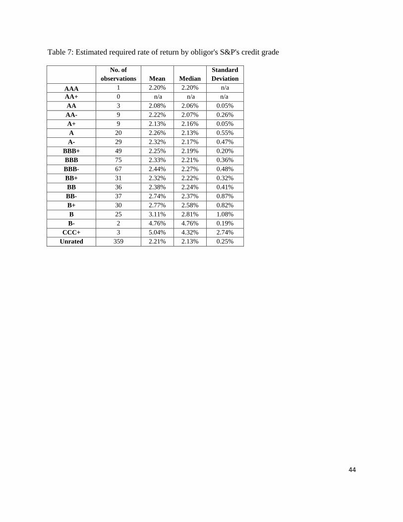
44

Table 7: Estimated required rate of return by obligor's S&P's credit grade

No. of observations Mean Median

Standard Deviation

AAA 1 2.20% 2.20% n/a AA+ 0 n/a n/a n/a AA 3 2.08% 2.06% 0.05% AA- 9 2.22% 2.07% 0.26% A+ 9 2.13% 2.16% 0.05% A 20 2.26% 2.13% 0.55% A- 29 2.32% 2.17% 0.47%

BBB+ 49 2.25% 2.19% 0.20% BBB 75 2.33% 2.21% 0.36% BBB- 67 2.44% 2.27% 0.48% BB+ 31 2.32% 2.22% 0.32% BB 36 2.38% 2.24% 0.41% BB- 37 2.74% 2.37% 0.87% B+ 30 2.77% 2.58% 0.82% B 25 3.11% 2.81% 1.08% B- 2 4.76% 4.76% 0.19%

CCC+ 3 5.04% 4.32% 2.74% Unrated 359 2.21% 2.13% 0.25%

45

Table 8: Estimated RAROC hurdle rates and the minimum required dollar amounts of expected income for the top 20 obligors by allocated capital

Name Ticker RAROC

hurdle rate Required income ($)

GOLDMAN SACHS GROUP INC GS 4.33% 3,201,190 BANK OF NOVA SCOTIA BNS 4.79% 2,684,665 TORONTO DOMINION BANK TD 4.29% 2,454,492 PRUDENTIAL FINANCIAL INC PRU 8.89% 1,745,956 WELLS FARGO & CO WFC 5.32% 2,456,725 METLIFE INC MET 9.01% 1,736,834 AFLAC INC AFL 6.79% 2,121,605 NELNET INC NNI 24.07% 3,490,103 CNO FINANCIAL GROUP INC CNO 9.03% 1,756,885 FBL FINANCIAL GROUP INC-CL A FFG 10.71% 1,574,690 UNITED CONTINENTAL HLDGS INC UAL 10.42% 1,878,891 EDISON INTERNATIONAL EIX 6.15% 1,175,403 SYNOVUS FINANCIAL CORP SNV 10.61% 1,584,521 NASDAQ OMX GROUP INC NDAQ 13.66% 1,805,530 ASSURANT INC AIZ 8.80% 1,446,979 CMS ENERGY CORP CMS 7.97% 1,119,811 AMERICAN EXPRESS CO AXP 4.73% 2,180,940 FIRSTENERGY CORP FE 5.89% 1,217,012 UNITED STATES STEEL CORP X 12.08% 1,401,282 MANULIFE FINANCIAL CORP MFC 5.65% 1,049,979 TOTAL PORTFOLIO 8.28% 359,539,481

46

Table 9: Top 20 debt instruments by profitability ranking: Instrument-specific hurdle rate vs. uniform hurdle rate

Ticker Name

Using instrument-specific hurdle rate

Using (uniform) weighted average hurdle rate

Ranking Excess return Ranking Excess return SXT SENSIENT TECHNOLOGIES CORP 1 74.40% 1 72.93% CVH COVENTRY HEALTH CARE INC 2 39.29% 2 42.03% RL RALPH LAUREN CORP 3 37.08% 3 36.32%

CVG CONVERGYS CORP 4 34.90% 4 34.66% DGX QUEST DIAGNOSTICS INC 5 31.87% 5 31.71% FIS FIDELITY NATIONAL INFO SVCS 6 30.44% 6 28.77% HPT HOSPITALITY PROPERTIES TRUST 7 28.46% 7 26.99% CL COLGATE-PALMOLIVE CO 8 24.24% 10 21.96%

UVV UNIVERSAL CORP/VA 9 23.66% 9 24.48% HRB BLOCK H & R INC 10 22.39% 8 24.84% RKT ROCK-TENN CO 11 21.14% 12 20.56%

A AGILENT TECHNOLOGIES INC 12 20.51% 14 19.17% WPI WATSON PHARMACEUTICALS INC 13 19.22% 17 16.92% DF DEAN FOODS CO 14 18.75% 11 20.66% G GENPACT LTD 15 18.20% 15 18.35%

WEN WENDY'S CO 16 17.16% 13 19.62% EQY EQUITY ONE INC 17 16.70% 18 16.48% CPB CAMPBELL SOUP CO 18 16.50% 19 15.47% DAR DARLING INTERNATIONAL INC 19 15.99% 16 17.21% DDS DILLARDS INC -CL A 20 15.12% 20 14.66%

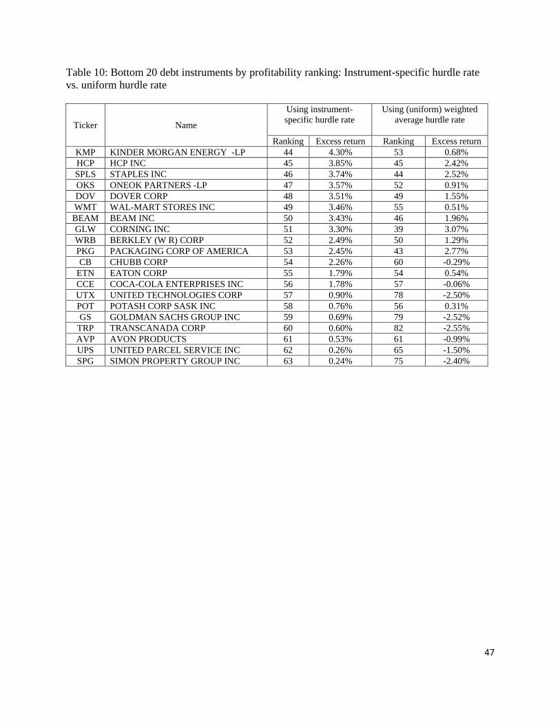
47

Table 10: Bottom 20 debt instruments by profitability ranking: Instrument-specific hurdle rate vs. uniform hurdle rate

Ticker Name

Using instrument-specific hurdle rate

Using (uniform) weighted average hurdle rate

Ranking Excess return Ranking Excess return KMP KINDER MORGAN ENERGY -LP 44 4.30% 53 0.68% HCP HCP INC 45 3.85% 45 2.42% SPLS STAPLES INC 46 3.74% 44 2.52% OKS ONEOK PARTNERS -LP 47 3.57% 52 0.91% DOV DOVER CORP 48 3.51% 49 1.55% WMT WAL-MART STORES INC 49 3.46% 55 0.51% BEAM BEAM INC 50 3.43% 46 1.96% GLW CORNING INC 51 3.30% 39 3.07% WRB BERKLEY (W R) CORP 52 2.49% 50 1.29% PKG PACKAGING CORP OF AMERICA 53 2.45% 43 2.77% CB CHUBB CORP 54 2.26% 60 -0.29%

ETN EATON CORP 55 1.79% 54 0.54% CCE COCA-COLA ENTERPRISES INC 56 1.78% 57 -0.06% UTX UNITED TECHNOLOGIES CORP 57 0.90% 78 -2.50% POT POTASH CORP SASK INC 58 0.76% 56 0.31% GS GOLDMAN SACHS GROUP INC 59 0.69% 79 -2.52%

TRP TRANSCANADA CORP 60 0.60% 82 -2.55% AVP AVON PRODUCTS 61 0.53% 61 -0.99% UPS UNITED PARCEL SERVICE INC 62 0.26% 65 -1.50% SPG SIMON PROPERTY GROUP INC 63 0.24% 75 -2.40%

48

Figure 1: Mean required rate of return by obligor's S&P's credit grade

2.00%

2.50%

3.00%

3.50%

4.00%

4.50%

5.00%

5.50%

-

200

400

600

800

1,000

1,200

1,400

1,600

1,800

2,000

Requ

ired

Rate

of R

etur

n

Expo

sure

($M

)

Exposure Required Rate of Return

49

Figure 2: Scatter-plot of the profitability rankings based on the naive approach of using a single portfolio-wide hurdle rate against those from the use of instrument-specific hurdle rate.

0102030405060708090

100110120

0 10 20 30 40 50 60 70 80 90 100 110 120

Rank

ing

base

d on

wei

ghte

d av

erag

e hu

rdle

rate

Ranking based on instrument-specific hurdle rate

50

Appendix A: Additional statistics of the sample portfolio Table A1: Number of debt issuers by industry sectors

Sector No. of observations % of

observations Financial Sector 151 19.24%

Commercial Banks 36 4.59% Funds 60 7.64%

Insurance 32 4.08% Other Non-Bank FI 17 2.17% Financial Services 6 0.76%

Business Service 99 12.61% Oil & Gas 68 8.66%

Oil & Gas, Exploration 60 7.64% Oil & Gas, Refining 8 1.02%

Utilities 46 5.86% Chemicals 49 6.24% Retail & Wholesale 38 4.84% Consumer Durables 36 4.59% Aerospace & Defence 41 5.22% Telecoms 20 2.55% Automotive 20 2.55% Equipment 31 3.95% Machinery & Equipment 31 3.95% Rail & Water Transportation 16 2.04% Food Manufacturing 15 1.91% Metal Products 20 2.55% Paper Products 11 1.40% Medical Services 10 1.27% Mining 17 2.17% Construction 9 1.15% Entertainment 8 1.02% Real Estate 8 1.02% Hotels & Restaurants 11 1.40% Land Transport 4 0.51% Air Transport 3 0.38% Clothing Manufacturing 9 1.15% Consumer Services 4 0.51% Agriculture 3 0.38% Automotive Rental 2 0.25% Publishing 1 0.13% Food Retail & Wholesale 2 0.25% Forestry 1 0.13% Tobacco 1 0.13%

Total 785 100%

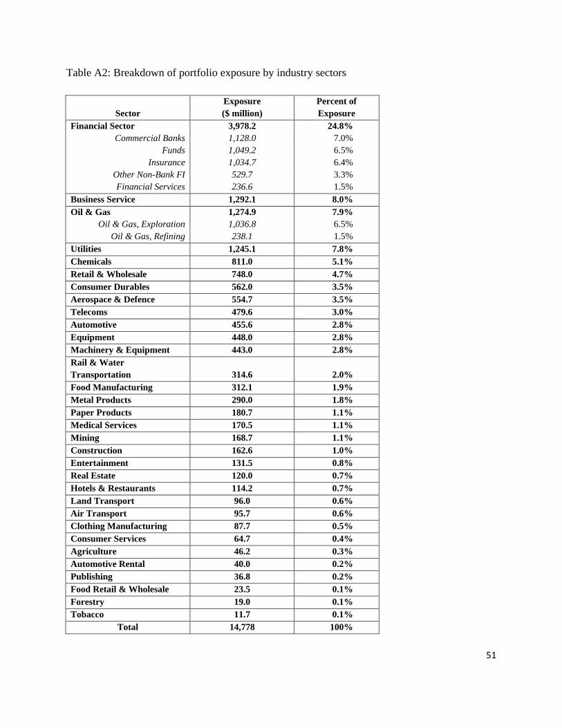
51

Table A2: Breakdown of portfolio exposure by industry sectors

Sector Exposure ($ million)

Percent of Exposure

Financial Sector 3,978.2 24.8% Commercial Banks 1,128.0 7.0%

Funds 1,049.2 6.5% Insurance 1,034.7 6.4%

Other Non-Bank FI 529.7 3.3% Financial Services 236.6 1.5%

Business Service 1,292.1 8.0% Oil & Gas 1,274.9 7.9%

Oil & Gas, Exploration 1,036.8 6.5% Oil & Gas, Refining 238.1 1.5%

Utilities 1,245.1 7.8% Chemicals 811.0 5.1% Retail & Wholesale 748.0 4.7% Consumer Durables 562.0 3.5% Aerospace & Defence 554.7 3.5% Telecoms 479.6 3.0% Automotive 455.6 2.8% Equipment 448.0 2.8% Machinery & Equipment 443.0 2.8% Rail & Water Transportation 314.6 2.0% Food Manufacturing 312.1 1.9% Metal Products 290.0 1.8% Paper Products 180.7 1.1% Medical Services 170.5 1.1% Mining 168.7 1.1% Construction 162.6 1.0% Entertainment 131.5 0.8% Real Estate 120.0 0.7% Hotels & Restaurants 114.2 0.7% Land Transport 96.0 0.6% Air Transport 95.7 0.6% Clothing Manufacturing 87.7 0.5% Consumer Services 64.7 0.4% Agriculture 46.2 0.3% Automotive Rental 40.0 0.2% Publishing 36.8 0.2% Food Retail & Wholesale 23.5 0.1% Forestry 19.0 0.1% Tobacco 11.7 0.1%

Total 14,778 100%

52

Table A3: Top 30 obligors by exposure

Ticker Company Name Ratings

Industry Exposure

($M)

S&P's Moody’s GS GOLDMAN SACHS GROUP INC A A1 Non-Bank FI 130.7

WFC WELLS FARGO & CO AA- A2 Commercial Bank 99.5 BNS BANK OF NOVA SCOTIA AA- Aa1 Commercial Bank 99.5 TD TORONTO DOMINION BANK AA- Aaa Commercial Bank 99.5 AXP AMERICAN EXPRESS CO BBB+ A3 Finance 97.6 WMT WAL-MART STORES INC AA Aa2 Retail & Wholesale 94.3 AFL AFLAC INC A- A3 Insurance 74.1 COP CONOCOPHILLIPS A A1 Oil & Gas, Refining 71.1 DFS DISCOVER FINANCIAL SVCS INC BBB- Ba1 Finance 65.8 ADP AUTOMATIC DATA PROCESSING AAA Aaa Business Service 64.9 KFT KRAFT FOODS INC BBB Baa2 Food Manufacturing 63.3 ICE INTERCONTINENTALEXCHANGE INC

Non-Bank FI 57.5

UTX UNITED TECHNOLOGIES CORP A A2 Automotive 56.4 ABT ABBOTT LABORATORIES AA A1 Chemicals 56.0 DOW DOW CHEMICAL BBB Baa3 Chemicals 55.1 BLK BLACKROCK INC A+ A1 Non-Bank FI 54.6 UAL UNITED CONTINENTAL HLDGS INC B B3 Air Transport 52.5 CB CHUBB CORP A+ A2 Insurance 52.0 ORCL ORACLE CORP A A1 Business Service 51.1 TGT TARGET CORP A+ A2 Retail & Wholesale 50.4 WLP WELLPOINT INC A- Baa1 Insurance 48.5 S SPRINT NEXTEL CORP BB- B2 Telecoms 48.5 NEE NEXTERA ENERGY INC A- Baa1 Utilities 47.9 CVS CVS CAREMARK CORP BBB+ Baa2 Retail & Wholesale 47.8 CNO CNO FINANCIAL GROUP INC B+ B2 Insurance 47.2 HON HONEYWELL INTERNATIONAL INC A A2 Automotive 47.0 SO SOUTHERN CO A Baa1 Utilities 47.0 LMT LOCKHEED MARTIN CORP A- Baa1 Automotive 46.7 SU SUNCOR ENERGY INC BBB+ Baa2 Oil & Gas, Refining 46.7 VLO VALERO ENERGY CORP BBB Baa2 Oil & Gas, Refining 45.8 All Other Exposure 12,858.9 Total 14,778.0