DETERMINATION OF OPTIMAL PRODUCTION PROCESS USING ...

Int j simul model 17 (2018) 4, 609-622

ISSN 1726-4529 Original scientific paper

https://doi.org/10.2507/IJSIMM17(4)447 609

DETERMINATION OF OPTIMAL PRODUCTION PROCESS

USING SCHEDULING AND SIMULATION SOFTWARE

Duplakova, D.*; Teliskova, M.; Duplak, J.; Torok, J.; Hatala, M.; Steranka, J. & Radchenko, S.

Technical University of Kosice, Faculty of Manufacturing Technologies with a seat in Presov,

Bayerova 1, 080 01 Presov, Slovakia

E-Mail: [email protected] (* Corresponding author)

Abstract

The objective of the article is to present the linking of simulation and planning software. The paper

begins with a review of recent literature as well as description of the problem under investigation.

Following from practical requirements, five decision-making rules were implemented to the

production process. In the final part, the overall results to ensure time and economic efficiency of the

production process are presented. The obtained results show that the best option is to apply the rule

during which the first part to be machined is the one that first enters the production process to ensure

minimum production time, maximum machine load and limit machine costs. By application of this

rule, the total production time accounts for 524 seconds at the total cost of 7914.60 €. The overall

benefits of the research are being described in details in the final part of the article. (Received in April 2018, accepted in July 2018. This paper was with the authors 1 week for 1 revision.)

Key Words: Simulation Software, Scheduling Software, Time Efficiency, Economic Efficiency

1. INTRODUCTION

Nowadays, simulation software is being widely used in various industries. Simulation tools

are applied in construction industry, mining industry, electrical engineering, automotive

industry and general engineering. In engineering and automotive industry, simulation tools

can be applied to production and auxiliary processes, logistics, planning, construction,

management, etc. Logistics, planning and management are the areas in which simulation tools

are used very often. Various supporting planning and simulation tools are used in this field to

ensure optimal running of the production process both technically and economically. For this

reason, it is necessary to focus the research activities on the issue within the scientific

community. It is generally known that optimization ensures economic and logistic efficiency

of production necessary for the smooth running of each manufacturing enterprise. Due to the

large number of simulation tools that can be used in manufacturing plants, Rashidi describes

six basic taxonomies as well as compares over 60 simulation tools in the taxonomies [1]. A

large number of existing studies in the broader literature have examined the issue of material

flow planning and simulation. In 2014, the Journal of System and Software released the

publication which provided an overview of the research carried out in the area of industrial

application of simulation tools [2]. In 1997, modern Witness simulation tool was presented

and described at the Atlanta Conference. This tool was applied to various optimization

processes [3]. In 2011, Witness Simulation Tool was used to solve logistics problems in

automotive components manufacturing. The solution to the problem was to optimize planning

and layout of the existing system followed by the general conclusion as well as

recommendation for small and medium-sized enterprises aimed at automotive components

production [4]. In 2012, optimization of the parameters of the Kanban production system

focusing on the assembly site using this simulation tool was resolved [5].

In 2013, the wide-scale application of this simulation tool was proved. Witness simulation

tool was used to create a universal simulation model for verification and subsequent

optimization of handling devices using basic heuristic optimization methods [6]. In 2014, the

https://doi.org/10.2507/IJSIMM17(4)447

mailto:[email protected]

Duplakova, Teliskova, Duplak, Torok, Hatala, Steranka, Radchenko: Determination of …

610

authors Chen et al. utilized the simulation tool to shorten production cycles in developing a

new product [7], and a year later, Dyntar and Strachotova applied this tool to design and

optimize the supply chain [8]. In 2016, research on using Witness program was aimed at

improving material flow continuity [9], planning and layout optimization [10] etc. The

literature review shows that the application of the simulation tool is used not only in

industries but it is possible to apply Witness simulation tool to education process. The authors

Cotet et al. utilized CAD simulation and material flow simulation to create a platform for

educational purposes. Developing the platform enabled to identify and remove bottlenecks to

ensure high efficiency [11]. In 2017, Witness was used to solve the optimization of the

assembly line balancing in GA [12] based production as well as to improve productivity in a

small manufacturing enterprise [13]. In addition to the simulation tool used to optimize

material flow, various planning software programs are used in common practice to ensure

time and economic efficiency. A more comprehensive description can be found in the study

aiming at optimizing time structures using Lekin scheduling software. Using Gantt charts, the

authors set the optimal material flow arrangement to ensure time efficiency [14]. In 2017,

Forrai and Kulcsar issued the publication dedicated to the creation of the new planning

software to support automotive production focusing on creating plans to implement

manufacturing activities that meet customer requirements [15]. As has been previously

reported in the literature, planning issues can be applied in various simulation tools. The

authors bring some more information about the use of hybrid metaheuristic algorithm for job

shop scheduling problem in cooperation for subsequent verification with simulation tools

Simio and Autodesk Factory Design Suite [16]. Recent study by Coman and Burian

concluded that planning issues can also be addressed by using WinQSB and Lekin software

programs [17]. It is important to note that the issue of simulation tools and planning is

applicable not only in the field of material flow planning but also in ensuring economic

efficiency. A recent study by Gracanin et al. reviewed the impact of job shop scheduling on

value stream optimization and decreasing of cost-time investment [18]. It was reported in the

literature that the wide variety of simulation and scheduling software programs are used

separately. As far as we know, no previous research has investigated the issue of linking

simulation and planning software programs including the verification of its results. The idea

of linking both simulation and scheduling programs was based on a requirement to ensure an

optimal production process when taking into account both time and economic aspects.

2. MATERIAL AND METHODS

Two software programs – Lekin planning program and Witness simulation program were

applied in the research. The input values of the production times of inner rings, which are part

of the rolling bearings (P1 – P4), were obtained from the practice. Specific quantitative data is

shown in Table I. The columns represent the individual manufacturing operations and the

rows include the manufactured components. Values are given in seconds. Fig. 1 below the

input values table shows the material flow. To meet the practical requirements, preference

was given to individual component machining. The parts are suitable to be machined in the

following order: P1, P2, P3, and P4.

Lekin Planning Software was used to create optimal ordering for individual component

machining using Gantt Charts. Job shop planning was chosen for the appearance of the given

production process. The nm minimum-makespan general job-shop scheduling problem can

be described by a set of n jobs {Ji} (1 ≤ j ≤ n) which is to be processed on a set of m machines

{Mr} (1 ≤ r ≤ m). Each job has a technological sequence of machines to be processed [19].


611

Table I: Input data.

Operation P1 [s] P2 [s] P3 [s] P4 [s]

Grinding 1 - 3 21 3

Roughing 1 26 - - -

Chamfering 3 - 14 4

Roughing 2 - 15 17 16

Turning 3 - - -

Grinding 2 - 4 43 47

Grinding 3 - - 37 38

Grinding 4 - - - 49

Burnishing 30 44 41 55

Markings 12 22 45 18

Cleaning 1 30 30 30 30

Final degreasing 7 3 3 3

Cleaning 2 30 30 30 30

Transport 107 96 125 133

Figure 1: Material flow.

Figure 2: Example of a directed graph for job shop with makespan as objective [20].

For this type of planning, five heuristic rules were applied to create an optimal production

process considering the practical requirements. These rules are the part of Lekin program. In

each mathematical expression of the rules, the following notations are used:

N(t) – a set of waiting jobs at time t Ij(t) – priority index of job j N(t)

rj – release date of job j N(t) pj – processing time of job j N(t)

dj – due date of job j N(t)

wj – importance factor (or weight) of job j N(t)

vj – remaining processing time of job j N(t) (0 ≤ vj(t) ≤ pj)

p′qj – processing time of the operation of job j, which corresponds to a certain pij value

according to the machine I on which operation q is to be processed.

The following dispatching rules are to be used:

1. The shortest processing time rule (SPT) generates an optimal schedule for a single

machine scheduling problem which minimizes the total completion time. The priority index Ij

of job j is defined by:


612

(1)

2. First Come – First Served (FCFS) – the jobs are fulfilled in arrival order to

manufacturing process. This rule arranges the jobs in N(t) in non-decreasing order of rj. The

priority index Ij of job j is defined by:

(2)

3. Minimum slack rule (MS) is usable in manufacturing planning for minimization of idle

time between workstations. The main principle consists in job preference with the higher

processing demand by slack time. The priority index Ij of job j is defined by:

(3)

4. Critical Ratio rule (CR) – in practice, a job is critical if the slack time is relatively small

and its importance factor (wj) is relatively large. The priority index Ij(t) of job j (dj > t) is

defined by:

(4)

5. Longest processing time rule (LPT) – preferred operation of part with the longest cycle

time. The priority index Ij of job j is defined by:

(5)

In the second part of the experiment, Witness software was used to verify the decision-

making rules as well as to determine the optimal organization of the production process not

only in terms of time efficiency but also in terms of its economic efficiency. Based on

material flow that is described above, a basic model has been developed using Witness

software which was subsequently modified on the basis of time-based optimization in Lekin

scheduling program. Fig. 3 shows the simulation model.

Figure 3: Model of production process – Witness software.

3. APPLICATION OF SCHEDULING SOFTWARE LEKIN AND

SIMULATION SOFTWARE WITNESS

Based on the input data, five Gantt charts were created with the descriptions of the

arrangements. In individual arrangements and evaluations, it is necessary to focus on the

following variables:

j

jp

I1

j

jr

I1

))((

1

ttvdI

jj

j

)()(

td

wtI

j

j

j

´max qjj pI


613

The Makespan (Cmax) – the maximum job completion time. A job's completion time Cj is

the time it finishes its processing under a given schedule.

The Maximum Tardiness (Tmax). A job's tardiness Tj is the positive part of the difference

between its completion time Cj and its due date dj: Tj = (Cj – dj). For each job j, Uj is

defined as an indicator of its lateness: Uj = 1 if job j is late, and 0 otherwise.

The Total Number of Late Jobs (ΣUj).

The Total Flow Time (ΣCj) – the sum of job completion times.

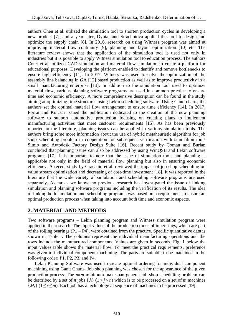
When applying the SPT rule, care must be taken to minimize production time. Fig. 4

provides a basic Gantt chart with individual sequences and operations that meet the

requirement to minimize production time. The total Cmax production time in this case reached

543 seconds with a total Tmax delay of 117 seconds. In a Gannt chart we can see the order of

individual component processing, where P1 and P2 are the first components to leave the

warehouse to be machined in the production process. In this case, on each machine, the last

component to be machined is P4 which also exits the overall production process as the last

one. When applying the SPT rule, a total of three late jobs, was recorded.

Figure 4: Gantt charts – SPT rule.

When applying the second FCFS rule, in contrast to applying the SPT rule, the difference

lies in the arrangement only during the Chamfering operation, where P3 is the first part to be

machined followed by P3 and P4 (Fig. 5). In this case, shorter production time is obtained

when applying the first rule but the preference of task processing is violated. The total

production time when applying the second rule accounts for 524 seconds with a total Tmax

delay of 98. As with the first rule, three late jobs have been recorded.

Based on the requirement of minimum idle time between workstations, it is necessary to

ensure the maximum possible continuity of the production process. In this case, the MS rule

was applied with the maximum job completion Cmax time reaching 534 seconds with a delay

of 108 seconds (Fig. 6). However, the total flow time is the largest among all the applied rules

so far. As with previous rule applications, three late jobs have been recorded.


614

Figure 5: Gantt charts – FCFS rule.

Figure 6: Gantt charts – MS rule.

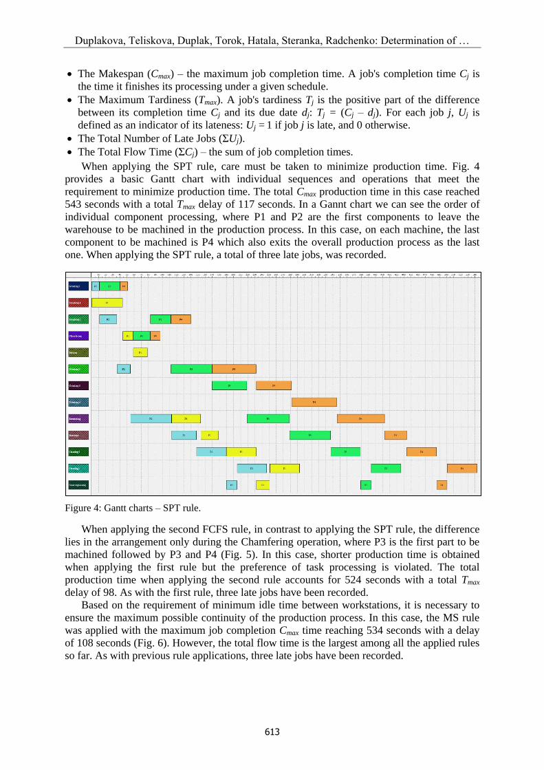
If the slack time is relatively small and its importance factor is relatively large then it is

important to use the CR rule. Once again in this application there occurs a change in order of

parts machining at the Chamfering workplace. This change is not very satisfactory since the

overall makespan Cmax has increased to 566 seconds with the highest increase in processing

delay of up to 140 seconds (Fig. 7).


615

Figure 7: Gantt charts – CR rule.

The last applied LPT rule organized the manufacturing process with the greatest changes

over the previous rules. This rule was chosen by the company to reduce production costs

during material supply delays. Consequently, the larger the total production time is for the

individual components the later it is possible to supply the material for further production.

Under LPT, the total production time was 541 seconds for up to four late jobs (Fig. 8). The

total delay lasted 294 seconds.

Figure 8: Gantt charts – LPT rule.

The overall results of the rules applied are presented in Fig. 9 with graphical

representation using the objective chart (Fig. 10). The values Cmax, Tmax and ∑Ui from all of

the presented values are important and decisive.


616

Figure 9: Log Book of applied rules.

Figure 10: Objective chart – graphical interpretation of the results.

Based on Gantt charts created by means of scheduling software, the models were designed

using Witness simulation tool to verify the applied decision rules and their subsequent

technical and economic evaluation.

Verification of the simulation model assembly was performed by monitoring the order of

individual components machining on the given machines and also through the total

production time. Five verification models were compiled according to each rule. Table II

shows the total production time achieved in Witness program when applying individual rules.

Table II: Total production time – Witness program.

Dispatching rule Production time [s]

SPT rule 543

FCFS rule 524

MS rule 534

CR rule 566

LPT rule 541

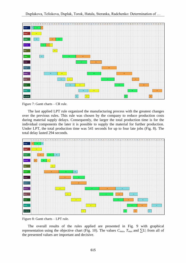
In addition to the total production time, the manufacturing time of the individual

components was also monitored. Partial component production time for each rule is shown in

Fig. 11.

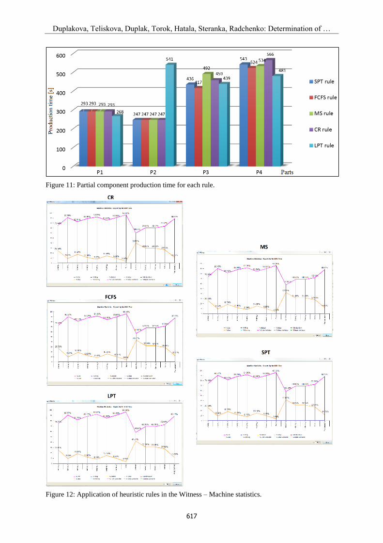
From the models that were created and in addition to the total production time and partial

production time of the individual components, the individual machines load has been also

monitored and recorded in the graphs below. Based on these charts, it can be stated that the

load and hence the inactivity of the machines in all cases reach values differing in tenths. Fig.

12 presents graphical results of machine load and inactivity after applying heuristic rules.


617

Figure 11: Partial component production time for each rule.

Figure 12: Application of heuristic rules in the Witness – Machine statistics.


618

Having verified the simulation model, the costs that can only be assessed using Witness

simulation software have been estimated. The Table III sets out the input values for the

subsequent implementation of the economic assessment ensuring the economic efficiency of

the production process.

Table III: Input data for economic evaluation [€].

Operation fixed used busy use idle use use per operation

Grinding_1 0.35 0.20 0.30 0.50

Grinding_2 0.50 0.80 0.40 0.20

Grinding_3 0.70 0.60 0.10 0.50

Grinding_4 0.60 0.70 0.80 0.40

Roughing_1 0.40 0.30 0.35 1.00

Roughing_2 0.45 0.25 0.8 0.15

Chamfering 0.30 0.10 0.25 0.30

Turning 0.25 0.40 0.60 1.00

Burnishing 0.90 0.70 0.40 0.90

Cleaning_1 1.20 0.85 0.55 0.35

Cleaning_2 1.20 0.50 0.75 0.25

Markings 1.10 0.45 0.85 0.80

Final_degreasing 0.70 0.35 0.20 0.50

The above costs were defined for one component in Euros per production machine. As

with total production time, partial time, machine load and inactivity, the economic indicators

were monitored in all five models. Table IV shows total machine costs when implementing

individual rules.

Table IV: Total machine costs.

Rule Fixed By Use By Quantity Total

CR 4.895,90 € 3.654,65 € 18,05 € 8.568,60 €

LPT 4.679,65 € 3.495,90 € 18,05 € 8.193,60 €

SPT 4.696,95 € 3.508,60 € 18,05 € 8.223,60 €

MS 4.619,10 € 3.451,45 € 18,05 € 8.088,60 €

FCFS 4.532,60 € 3.363,95 € 18,05 € 7.914,60 €

Having applied both planning and simulation software, the results were evaluated in a

global perspective for each condition. The obtained results and their evaluation are presented

in the following subchapter of the article.

4. RESULTS AND DISCUSSION

Within the overall assessment of the production process, it is necessary to follow the total

load for individual machines from the technical as well as economic point of view. Table V

shows the machine load after applying the heuristic rules.

The Table V shows that the minimum machine load accounts for 3.53 % for turning

operations. This low load is caused by the fact that only one component is being machined

once on the machine. One of the options to maximize machine load is to ensure machining of

other parts on this machine by obtaining new orders for machining by turning technology with

respect to the primary production process, adherence to logistics and thus ensuring the

economy of the overall production process, either primary or secondary. Since the maximum

machine load is not half of the possible value, it is appropriate to apply the design to all


619

machines and thus to provide a secondary production process in the production plant, thereby

maximizing machine load and ensuring greater economic efficiency.

Table V: Busy state of machines.

Busy [%]

Operation CR LPT SPT MS FCFS

Grinding_2(1) 24.56 25.69 25.6 26.03 26.53

Grinding_1(1) 9.01 9.43 9.39 9.55 9.73

Grinding_3(1) 17.49 18.3 18.23 18.54 18.89

Grinding_4(1) 11.31 11.83 11.79 11.99 12.21

Roughing_1(1) 7.77 8.13 8.1 8.24 8.4

Roughing_2(1) 14.49 15.16 15.1 15.36 15.65

Chamfering(1) 9.36 9.8 9.76 9.93 10.11

Turning(1) 3.53 3.7 3.68 3.75 3.82

Burnishing(1) 39.93 41.77 41.62 42.32 43.13

Cleaning_1(1) 29.68 31.05 30.94 31.46 32.06

Cleaning_2(1) 29.68 31.05 30.94 31.46 32.06

Markings(1) 26.33 27.54 27.44 27.9 28.44

Final_degreasing(1) 11.31 11.83 11.79 11.99 12.21

The second observed parameter and practical requirement is to track the total production

time after applying the heuristic rules. As it is shown in Table III, the minimum

manufacturing time was reached after applying the FCFS rule of 524 seconds and the

maximum manufacturing time was reached when applying the CR rule.

Figure 13: Production time after the application of the rules

To ensure economic efficiency, the total cost, with the input values shown in Table V, was

also surveyed. After applying the individual rules, the total cost is shown in Fig. 14.

Figure 14: Economic of production process after the application of the rules.


620

Based on the above-mentioned chart of total costs after the implementation of the

decision-making rules in the production process, it can be stated that the total machine costs

are the highest when applying the CR rule. The lowest costs were recorded in the production

process after the FCFS rule was applied.

In the global assessment of overall research for the conditions set out in practice, the

following conclusions can be made:

In order to ensure a minimum production time (524 seconds), the best option is to apply

the FCFS rule to the existing production system in which the first component to be used is

the one that first enters the production process.

To ensure maximum machine load, it is appropriate to apply the FCFS rule, after which the

average machine load reached 19.48 %; due to the low average value it would be

appropriate to apply the proposed solution to the implementation of the secondary

production process at the workplace.

For the provision of limited machine costs (practical requirement for maximum of €8000),

it is also appropriate to apply the FCFS rule resulting in total machine costs of €7914.60.

Based on these conclusions, it could be stated that the most appropriate application for the

given manufacturing process is to use the FCFS rule in terms of ensuring technical and

economic efficiency.

In the global assessment of the overall research for the general conditions resulting from

the research, the following conclusions can be made:

Creation of verification models in the simulation program based on background material

from the scheduling program.

The information provided should be used in planning and management of production

process.

Saving time and costs as a result of using planning and simulation tool at the same time.

Having linked both simulation and planning programs, the rapid possibility of designing

optimum production time and ensuring economic efficiency for the manufacturing process

in general is obvious.

More optimizations can be made to the created models saving both time and money for

manufacturing companies.

5. CONCLUSION

Nowadays, every manufacturing enterprise needs to produce the highest quality products in

the shortest possible time meeting all the requirements of the customer [21, 22]. To meet the

practical needs, planning has helped since ancient times. Production scheduling plays a vital

role in planning and operation of a manufacturing system [23]. The Job Shop Scheduling

Problem (JSSP) is one of the most general and difficult of all traditional scheduling

combinatorial problems with considerable importance in industry [24]. Today, we can

observe much pressure on enterprises from the market, the competition and the customer

[25, 26]. For this reason, various planning or simulation programs are becoming increasingly

important. Such programs enable various companies to handle difficult situations in

production processes. The basic idea of our investigation was the requirement to ensure the

optimal solution for the production process regarding both time and economy.

The requirement was solved by simulation due to non-recovery of the running production

process. The original benefit lies in linking both planning and simulation software. Planning

software provides material flow optimization in terms of time efficiency and the resulting

solutions are then verified using simulation software that optimizes material flow in terms of

economic efficiency. From a practical point of view, this paper can be viewed as an important

presentation of linking both simulation and planning software programs that can be used by


621

every manufacturing company that needs to optimize its existing or newly created production

process taking into account both time and economic aspects.

ACKNOWLEDGEMENT

This work was supported by the research grants VEGA 1/0492/16 – Research of the Possibilities of

Elimination Deformations of the Thin Components with the Use of High Speed Machining and KEGA

025TUKE-4/2018 – Transfer of new approaches of teaching technology-oriented courses and

implementation of teaching in practical terms for current needs of the Slovak industry.

REFERENCES

[1] Rashidi, H. (2017). Discrete simulation software: a survey on taxonomies, Journal of Simulation,

Vol. 11, No. 2, 174-184, doi:10.1057/jos.2016.4

[2] Ali, N. B.; Petersen, K.; Wohlin, C. (2014). A systematic literature review on the industrial use of

software process simulation, Journal of Systems and Software, Vol. 97, 65-85,

doi:10.1016/j.jss.2014.06.059

[3] Markt, P. L.; Mayer, M. H. (1997). WITNESS simulation software: a flexible suite of simulation

tools, Proceedings of the 29th Winter Simulation Conference (WSC'97), 711-717,

doi:10.1145/268437.268613

[4] Zhou, R.; Zhao, H.; Chen, K. (2011). Production logistics system simulation about automobile

parts shop based on Witness and E-factory, Advanced Materials Research, Vols. 291-294, 3175-

3179, doi:10.4028/www.scientific.net/AMR.291-294.3175

[5] Xiao, Y.; Li, Y. Y.; Zhou, K. Q. (2012). Parameter optimization of Kanban production system for

an engine assembly workshop based on Witness, Advanced Materials Research, Vol. 382, 252-

255, doi:10.4028/www.scientific.net/AMR.382.252

[6] Holík, J.; Landryová, L. (2013). Universal simulation model in Witness software for verification

and following optimization of the handling equipment, Emmanouilidis, C.; Taisch, M.; Kiritsis,

D. (Eds.), Advances in Production Management Systems. Competitive Manufacturing for

Innovative Products and Services, APMS 2012, Vol. 397, Springer, Berlin, 445-451,

doi:10.1007/978-3-642-40352-1_56

[7] Chen, Y. H.; Li, H. F.; Qiu, F. S.; Xu, J.; Feng, Z. T. (2014). Study on the product development

process based on WITNESS Simulation, Applied Mechanics and Materials, Vol. 577, 1292-1295,

doi:10.4028/www.scientific.net/AMM.577.1292

[8] Dyntar, J.; Strachotova, D. (2015). Witness dynamic simulation for supply chain design and

optimisation, Proceedings of the 26th International-Business-Information-Management-

Association Conference: Innovation management and sustainable economic competitive

advantage: from regional development to global growth, 346-351

[9] Zwolińska, B.; Smolińska, K. (2015). Use of Witness simulation for improving the continuity of

the flow, Conference Proceedings of the Carpathian Logistics Congress 2015, 485-490

[10] Ma, L.; Ma, M.; Ma, C.; Deng, J.; Liu, X.; Zhao, L. (2016). Simulation and optimization study on

layout planning of plant factory based on WITNESS, International Journal of Security and its

Applications, Vol. 10, No.5, 275-282

[11] Cotet, C. E.; Popa, C. L.; Enciu, G.; Popescu, A.; Dobrescu, T. (2016). Using CAD and flow

simulation for educational platform design and optimization, International Journal of Simulation

Modelling, Vol. 15, No. 1, 5-15, doi:10.2507/IJSIMM15(1)1.310

[12] Wang, Y.; Yang, O. (2017). Research on industrial assembly line balancing optimization based

on genetic algorithm and Witness simulation, International Journal of Simulation Modelling,

Vol. 16, No. 2, 334-342, doi:10.2507/IJSIMM16(2)CO8

[13] Jaffrey, V.; Mohamed, N. M. Z. N.; Rose, A. N. M. (2017). Improvement of productivity in low

volume production industry layout by using Witness simulation software, IOP Conference

Series: Materials Science and Engineering, Vol. 257, Paper 012030, doi:10.1088/1757-

899X/257/1/012030

https://doi.org/10.1057/jos.2016.4

https://doi.org/10.1016/j.jss.2014.06.059

https://doi.org/10.1145/268437.268613

https://doi.org/10.4028/www.scientific.net/AMR.291-294.3175

https://doi.org/10.4028/www.scientific.net/AMR.382.252

https://doi.org/10.1007/978-3-642-40352-1_56

https://doi.org/10.4028/www.scientific.net/AMM.577.1292

https://doi.org/10.2507/IJSIMM15(1)1.310

https://doi.org/10.2507/IJSIMM16(2)CO8

https://doi.org/10.1088/1757-899X/257/1/012030

https://doi.org/10.1088/1757-899X/257/1/012030


622

[14] Balog, M.; Dupláková, D.; Szilágyi, E.; Mindas, M.; Knapčíková, L. (2016). Optimization of

time structures in manufacturing management by using scheduling software Lekin, TEM Journal,

Vol. 5, No. 3, 319-323, doi:10.18421/TEM53-11

[15] Forrai, M. K.; Kulcsár, G. (2017). A new scheduling software for supporting automotive

component manufacturing, Jármai, K.; Bolló, B. (Eds.), Vehicle and Automotive Engineering,

Springer, Cham, 257-274, doi:10.1007/978-3-319-51189-4_25

[16] Zhang, H.; Liu, S.; Moraca, S.; Ojstersek, R. (2017). An effective use of hybrid metaheuristics

algorithm for job shop scheduling problem, International Journal of Simulation Modelling, Vol.

16, No. 4, 644-657, doi:10.2507/IJSIMM16(4)7.400

[17] Amariei, O. I.; Hamat, C. O.; Coman, L.; Burian, R. (2013). Minimizing makespan in job shop

production using a network approach, Robotica & Management, Vol. 18, No. 2, 39-41

[18] Gracanin, D.; Lalic, B.; Beker, I.; Lalic, D.; Buchmeister, B. (2013). Cost-time profile simulation

for job shop scheduling decisions, International Journal of Simulation Modelling, Vol. 12, No. 4,

213-224, doi:10.2507/IJSIMM12(4)1.237

[19] Yamada T; Nakano R. (1997). Job-shop scheduling, Zalzala, A. M. S.; Fleming, P. J. (Eds.),

Genetic algorithms in engineering systems, IEE Control Engineering series 55, The Institution of

Electrical Engineers, London, 134-160

[20] Pinedo, M. (2010). Scheduling: Theory, Algorithms, and Systems. New York University, New

York

[21] Lehocká, D.; Hlavatý, I.; Hloch, S. (2016). Rationalization of material flow in production of

semitrailer frame for automotive industry, Technical Gazette, Vol. 23, No. 4, 1215-1220,

doi:10.17559/TV-20131113100109

[22] Petru, J.; Zlamal, T.; Cep, R.; Pavlica, M. (2014). The using of elements of lean production to

increase efficiency and competitiveness of organizations in the engineering industry, Fourth

International Conference on Industrial Engineering and Operations Management, 802-811.

[23] Rathinam, B.; Govindan, K.; Neelakandan, B.; Raghavan, S. S. (2015). Rule based heuristic

approach for minimizing total flow time in permutation flow shop scheduling, Technical Gazette,

Vol. 22, No. 1, 25-32, doi:10.17559/TV-20130704132725

[24] Janes, G.; Perinic, M.; Jurkovic, Z. (2017). Applying improved genetic algorithm for solving job

shop scheduling problems, Technical Gazette, Vol. 24, No. 4, 1243-1247, doi:10.17559/TV-

20150527133957

[25] Zajac, J.; Beraxa, P.; Michalik, P.; Botko, F.; Pollák, M. (2016). Simulation of weld elbows hot

forming process, International Journal of Modeling and Optimization, Vol. 6, No. 2, 77-80,

doi:10.7763/IJMO.2016.V6.507

[26] Kočiško, M.; Novák-Marcinčin, J.; Baron, P.; Dobránsky, J. (2012). Utilization of progressive

simulation software for optimization of production systems in the area of small and medium

companies, Technical Gazette, Vol. 19, No. 4, 983-986

https://doi.org/10.18421/TEM53-11

https://doi.org/10.1007/978-3-319-51189-4_25



https://doi.org/10.17559/TV-20131113100109

https://doi.org/10.17559/TV-20130704132725

https://doi.org/10.17559/TV-20150527133957

https://doi.org/10.17559/TV-20150527133957

https://doi.org/10.7763/IJMO.2016.V6.507

DETERMINATION OF OPTIMAL PRODUCTION PROCESS USING ...

Documents

Transcript of DETERMINATION OF OPTIMAL PRODUCTION PROCESS USING ...