Determination of farmland values in New Zealand : the ...

DETERMINATION OF FARMLAND

VALUES IN NEW ZEALAND:

THE SIGNIFICANCE OF FINANCIAL LEVERAGE

G A Anderson

GAG Frengley

B D Ward

Research Report No. 209

April, 1991

Agribusiness and Economics Research UnitPO Box 84

Lincoln UniversityCANTERBURY

Telephone No: (64) (3) 252-811Fax No: (64) (3) 252-099

ISSN 0113-4485

AGRIBUSINESS & ECONOMICS RESEARCH UNIT

-The Agribusiness and Economics Research Unit (AERU) operatesfrqm Lincqln University pmvldlng research expertise for a widerange of organisations concerned with pmductlon, processing,distribution, finance and marketing,

The AERU operates as a semi-commercial research agency,Research contracts are carried out for clients on a commercialbasis and University research is supported by the AERU throughsponsorship of postgraduate research programmes, Researchclients Include Government Departments, both within NewZealand and from other countries, international agencies, NewZealand cqmpanies and organisations, individuals and farmers,Research results are presented through private client reports,where this is required, and through the publication systemoperated by the AERU, Two publication series are supported:Research Reports and Discussion Papers,

The AERU operates as a research co-ordinating body for theEconomics and Marketing Department and the Department ofFarm Management and Accounting and Valuation. This meansthat a total staff of approximately 50 professional people is potentially available to work on research projects. A wide diversityof expertise is therefore available for the AERU.

The major research areas supported by the AERU include tradepolicy, marketing (both institutional and consumer), accounting,finance, management, agricultural economics and rural sociology. In addition to the research activities, the AERU supportsconferences and seminars on topical issues and AERU staff areinvolved in a' wide range of professional and University relatedextension activities.

Founded as the Agricultural Economics Research Unit in 1962from an annual grant provided by the Department of Scientific andIndustrial Research (DSIR), the AERU has grown to become anindependent, major source of business and economic researchexpertise. DSIR funding was discontinued in 1986 and from April1987, in recognition of the development of a wider researchactivity in the agribusiness sector, the name of the organisationwas changed to the Agribusiness and Economics Research Unit.An AERU Management Committee comprised of the Principal, theProfessors of the three associate departments, and the AERUDirector and Assistant Director administers the general Unitpolicy.

AERU MANAGEMENT COMMITTEE 1991

Prolessor A C Bywater, B.Sc., Ph.D.(Professor of Farm Management)

Prolessor R H Juchau, B.Com., B.Ed., M.A.(Professor of Accounting and Finance)

AERU STAFF 1991

DirectorProfessor AC Zwart, B.Agr,Sc., M.Sc., Ph.D.

l\!lllllltant DirectorR L Sheppard, B.Agr.Sc. (Hons), B.B.S.

~tllleluch OllicersG Greer, B,Agr.Sc, (Hons)T P Grundy, B,Sc. (Hons), M,Com.

Prolessor A C Zwart, B.Agr.Sc., M.Sc., Ph.D.(Professor of Marketing)

R L Sheppard, B.Agr.Sc. (Hans), B.B.S.(Assistant Director, AERU)

Research OfficersL. M. Urquhart, B.Com.(Ag), Dip.Com,J R Fairweather, B.Agr.Sc., BA, M,A., Ph.D.

Visiting Research FellowN C Keating, PhD.

SecretaryJ Clark

CONTENTS

LIST OF TABLES

LIST OF FIGURES

PREFACE

ACKNOWLEDGEMENTS

SUMMARY

CHAPTER 1 INTRODUCTION

CHAPTER 2 LAND PRICE ISSUES

(iii)

(v)

(vii)

(ix)

1

2

2.1

2.2

A Review of Farm Asset Valuesand Returns, 1962-1987Factors Mfecting Farm AssetValue Fluctuations

5

8

CHAPTER 3 THE COMPETING THEORIES FOR LAND PRICE DETERMINATION 13

3.13.23.33.43.53.63.7

IntroductionNet Farm IncomeExpectations of InflationExpectations of Capital GainsThe Impact of Financial LeverageAccounting for Consumptive ValuesNew Zealand Research

13131517192021

CHAPTER 4 FINANCIAL LEVERAGE AS AN ALTERNATIVEDETERMINANT OF LAND PRICE: FINANCIAL LEVERAGE 25

4.14.24.34.4

4.5

IntroductionDefinition of the Farmland MarketThe Chosen MarketThe Land Price Equation4.4.1 Expected Net Rent4.4.2 The Impact of Financial Leverage4.4.3 The Impact of Debt Erosion4.4.4 SummaryAnalytical Procedure4.5.1 The Problem of Estimation4.5.2 An Alternative Method4.5.3 The Expected Impact of Financial Leverage

252526272829313233333435

4.6

4.7

Expectations4.6.1 Introduction4.6.2 The Treatment of Expectations4.6.3 Expectations of Returns to Total

Production Assets4.6.4 Expectations of Inflation

Definition of the Variables4.7.1 Proxy for Net Rent: Current

Returns to Total Production Assets4.7.2 Proxy for Land Value: The Value of

Total Production Assets "4.7.3 Proxy for the Inflation Rate:

The Consumer Price Index4.7.4 Proxy for the Rate of Income Tax:

The Highest Marginal Tax Rate4.7.5 Proxy for the Opportunity Cost of Equity:

Long Term Government Security Yields4.7.6 Proxy for the Cost of Debt: The Rural

Bank Mortgage Interest Rate4.7.7 Potential Problems With the Data

383839

4042

42

43

43

43

43

43

4343

CHAPTER 5 RESULTS OF THE ANALYSIS

5.1 Introduction5.2 Statistical Measures of Accuracy

5.2.1 Correlation Coefficient5.2.2 Theil's Inequality Coefficient

5.3 The Impact of Financial Leverage on FarmAsset Values, 1962-1987

5.4. The Hypothesized Changes in Debt LevelsBetween 1962 and 19875.4.1 Period 1: 1962-19685.4.2 Period 2: 1969-19775.4.3 Period 3: 1978-19835.4.4 Period 4: 1984-1987

CHAPTER 6 IMPLICATIONS FOR AGRICULTURAL POLICY

LIST OF REFERENCES

45

45454546

47

5151525454

57

59

LIST OF TABLES

5.1 Summary Results: Comparison of Actual and EstimatedSeries, 1962-1987 49





2.1

2.2

2.3

LIST OF FIGURES

N.Z.M.W.B.E.S. "All Classes Average"Current Returns and Capital Gains (Nominal Values)

N.Z.M.W.B.E.S. "All Classes Average"Current Returns and Capital Gains (Real Values)

N.Z.M.W.B.E.S. "All Classes Average"Value of Total Production Assets (Nominal and Real Values)

(iii)

6

7

9

PREFACE

Changes in the value of farmland have a significant impact on the returns which farmersachieve through their ownership of land and the entry and exit of people to and fromfarming. While the returns to farmers from actual farming activity have been considered toprovide a "poor return on investment" compared to other types of business investment, thereturn via capital gains has at least compensated for "lower" returns via income. The nontaxable nature of capital gain has in tum encouraged a higher proportion of the "ffumingreturn" into this area. However, analyses have shown that the increase in farmland capitalvalue has been greater than that which would be expected based upon actual and expectedfarm incomes.

The study presented in this Research Report provides evidence of the role of financialleverage in the establishment of farmland values. Where loan finance is available, increasesin capital values are recorded. The findings presented have significant implications foragricultural policy in that where actions are taken by Government or institutions to makefarm purchase finance more readily available, one of the significant outcomes is likely to bean increase in farmland prices.

This Research Report represents a significant contribution to the literature on farmlandvaluation.

G.A. Anderson is a Masterate Student in the Farm Management Department. (This ResearchReport is the published version of his Masterate Thesis.) Dr G.A.G. Frengley is a Reader inthe Farm Management Department and B.D. Ward is a Senior Lecturer in the Economics andMarketing Department.

A C ZwartDirector, AERU

(v)

ACKNOWLEDGEMENTS

The authors wish to recognise the financial assistance provided by the Policy ServicesDivision of the Ministry of Agriculture and Fisheries to complete this project.

(vii)

SUMMARY

An examination of the growth rates in farm asset values and returns in New Zealandbetween 1962 and 1987 reveals that a significant divergence has developed between the two.The value of nominal total production assets for the N.Z.M.W.B.E.S. 'All Classes Average'increased at an annual compound rate of 12.57 percent during the twenty five year periodwhile net income increased at a rate of only 9.33 percent. Moreover, a comparison of thecompound growth rates in real terms accentuates what Scholfield (1961) and Chryst (1965)termed the 'land price paradox', as farmland prices appeared to be increasing more rapidlythan increases in farm incomes seemed to warrant. Between 1972 and 1982 the real value oftotal production assets increased at an annual compound rate of 5.71 % despite the decreasein the real value of net farm income of 0.37% per annum.

In his study of farmland price determination, Seed (1986) points out that the historicalchanges in New Zealand farm values and incomes closely parallel the United Statesexperience during the 1962 -1987 period. As a result, many agricultural economists haveaddressed this apparent land price paradox, making some attempt to more accurately identifythe variables which have an impact on farm asset values. Although all accept the basicproposition that land rent is a key determinant of farmland value, numerous other casualvariables have been advanced. These include the impact of expected earnings growth onexpectation for capital gains which arises from farmland being treated as a speculativeinvestment, the possible impact of inflation on real farm values and an increase in theconsumptive demand for farmland.

However, the effect of financial leverage on land price variation has received relatively littleattention. The objective of this study was to examine the impact of financial leverage onfarmland price determination in New Zealand between 1962 and 1987.

Before constructing a land price model with which to test the hypothesized impact of debtfinance, a number of other important considerations were addressed. The first concerns theneed to identify a reasonably homogeneous land market on which to base the analysis. Burt(1986) suggests that many of the apparent difficulties of the existing empirical work areexacerbated by using aggregate data to analyze land prices. This may introduce suchproblems as extreme heterogeneity in land quality and the impact of non-agricultural valuesof farmland which are not reflected in current or historical land rents. Robison et al. (1985)also emphasize the need to identify and define a homogeneous market before selectingpossible price determinants. By doing so, the land value model may be able to moreprecisely incorporate the factors considered relevant to that individual market. Attemptingto pre-determine which factors are relevant in an aggregate market is obviously moredifficult.

The N.Z.M.W.B.E.S. class seven survey farm data was chosen as possibly the mosthomogeneous sample available within New Zealand. Examination of the New ZealandValuation Departments', classification of farm buyers indicates that the class seven farmlandarea is predominantly made up of single family units which are purchased for theirproductive use. As such, the possible impact of demand from consumptive users isconsidered small. The limited number of farm purchases by those classified as businessmenmay also suggest that the motive of anticipated capital gains has had a negligible influenceon farmland price determination in the class seven sample area.

Ox)

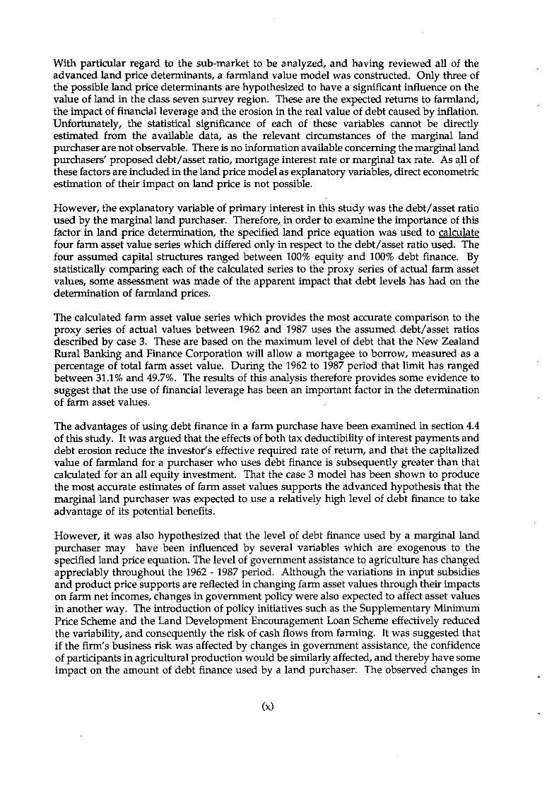
With particular regard to the sub-market to be analyzed, and having reviewed all of theadvanced land price determinants, a farmland value model was constructed. Only three ofthe possible land price determinants are hypothesized to have a significant influence on thevalue of land in the class seven survey region. These are the expected returns to farmland,the impact of financial leverage and the erosion in the real value of debt caused by inflation.Unfortunately, the statistical significance of each of these variables cannot be directlyestimated from the available data, as the relevant circumstances of the marginal landpurchaser are not observable. There is no information available concerning the marginal landpurchasers' proposed debt/asset ratio, mortgage interest rate or marginal tax rate. As ~ll ofthese factors are included in the land price model as explanatory variables, direct econometricestimation of their impact on land price is not possible.

However, the explanatory variable of primary interest in this study was the debt/asset ratioused by the marginal land purchaser. Therefore, in order to examine the importance of thisfactor in land price determination, the specified land price equation was used to calculatefour farm asset value series which differed only in respect to the debt/asset ratio used. Thefour assumed capital structures ranged between 100% equity and 100% debt finance. Bystatistically comparing each of the calculated series to the proxy series of actual farm assetvalues, some assessment was made of the apparent impact that debt levels has had on thedetermination of farmland prices.

The calculated farm asset value series which provides the most accurate comparison to theproxy series of actual values between 1962 and 1987 uses the assumed debt/asset ratiosdescribed by case 3. These are based on the maximum level of debt that the New ZealandRural Banking and Finance Corporation will allow a mortgagee to borrow, measured as apercentage of total farm asset value. During the 1962 to 1987 period that limit has rangedbetween 31.1 % and 49.7%. The results of this analysis therefore provides some evidence tosuggest that the use of financial leverage has been an important factor in the determinationof farm asset values.

The advantages of using debt finance in a farm purchase have been examined in section 4.4of this study. It was argued that the effects of both tax deductibility of interest payments anddebt erosion reduce the investor's effective required rate of return, and that the capitalizedvalue of farmland for a purchaser who uses debt finance is subsequently greater than thatcalculated for an all equity investment. That the case 3 model has been shown to producethe most accurate estimates of farm asset values supports the advanced hypothesis that themarginal land purchaser was expected to use a relatively high level of debt finance to takeadvantage of its potential benefits.

However, it was also hypothesized that the level of debt finance used by a marginal landpurchaser may have been influenced by several variables which are exogenous to thespecified land price equation. The level of government assistance to agriculture has changedappreciably throughout the 1962 - 1987 period. Although the variations in input subsidiesand product price supports are reflected in changing farm asset values through their impactson farm net incomes, changes in government policy were also expected to affect asset valuesin another way. The introduction of policy initiatives such as the Supplementary MinimumPrice Scheme and the Land Development Encouragement Loan Scheme effectively reducedthe variability, and consequently the risk of cash flows from farming. It was suggested thatif the firm's business risk was affected by changes in government assistance, the confidenceof participants in agricultural production would be similarly affected, and thereby have someimpact on the amount of debt finance used by a land purchaser. The observed changes in

(x)

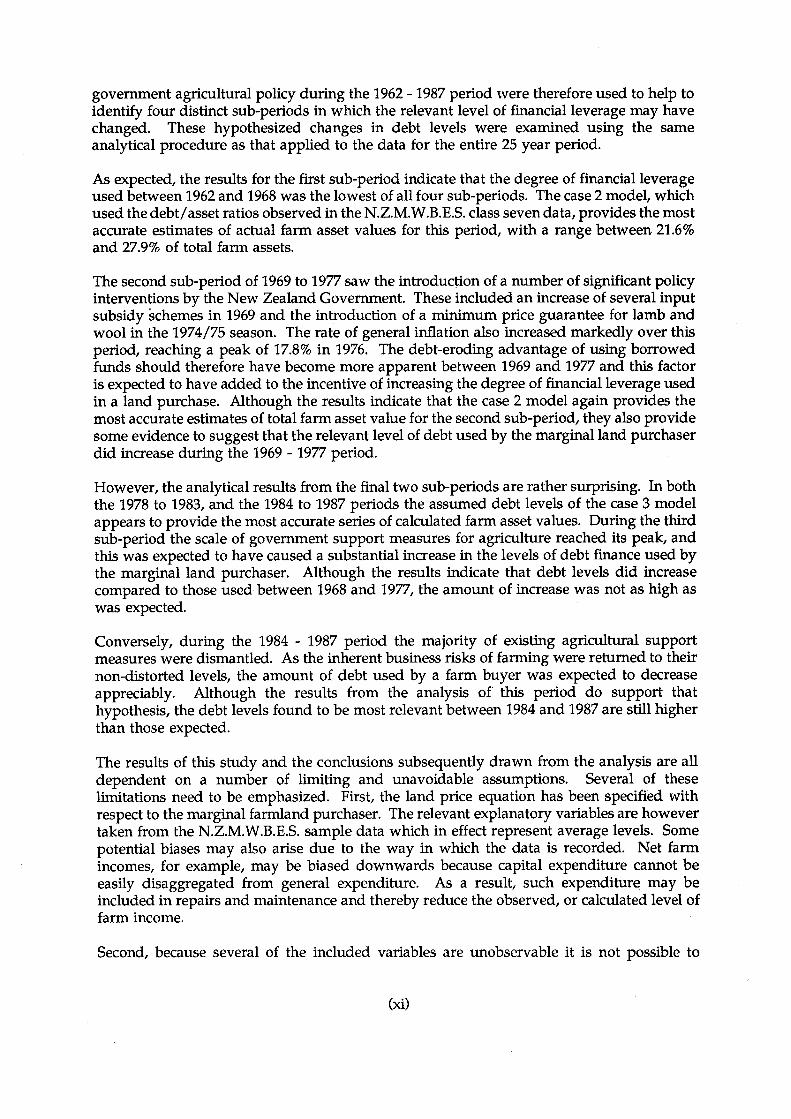
government agricultural policy dUring the 1962 - 1987 period were therefore used to help toidentify four distinct sub-periods in which the relevant level of financial leverage may havechanged. These hypothesized changes in debt levels were examined using the sameanalytical procedure as that applied to the data for the entire 25 year period.

As expected, the results for the first sub-period indicate that the degree of financial leverageused between 1962 and 1968 was the lowest of all four sub-periods. The case 2 model, whichused the debt/asset ratios observed in the N.Z.M.W.B.E.S. class seven data, provides the mostaccurate estimates of actual farm asset values for this period, with a range between 21.6%and 27.9% of total farm assets.

The second sub-period of 1969 to 1977 saw the introduction of a number of significant policyinterventions by the New Zealand Government. These included an increase of several inputsubsidy schemes in 1969 and the introduction of a minimum price guarantee for lamb andwool in the 1974/75 season. The rate of general inflation also increased markedly over thisperiod, reaching a peak of 17.8% in 1976. The debt-eroding advantage of using borrowedfunds should therefore have become more apparent between 1969 and 1977 and this factoris expected to have added to the incentive of increasing the degree of financial leverage usedin a land purchase. Although the results indicate that the case 2 model again provides themost accurate estimates of total farm asset value for the second sub-period, they also providesome evidence to suggest that the relevant level of debt used by the marginal land purchaserdid increase during the 1969 - 1977 period.

However, the analytical results from the final two sub-periods are rather surprising. In boththe 1978 to 1983, and the 1984 to 1987 periods the assumed debt levels of the case 3 modelappears to provide the most accurate series of calculated farm asset values. During the thirdsub-period the scale of government support measures for agriculture reached its peak, andthis was expected to have caused a substantial increase in the levels of debt finance used bythe marginal land purchaser. Although the results indicate that debt levels did increasecompared to those used between 1968 and 1977, the amount of increase was not as high aswas expected.

Conversely, during the 1984 - 1987 period the majority of existing agricultural supportmeasures were dismantled. As the inherent business risks of farming were returned to theirnon-distorted levels, the amount of debt used by a farm buyer was expected to decreaseappreciably. Although the results from the analysis of this period do support thathypothesis, the debt levels found to be most relevant between 1984 and 1987 are still higherthan those expected.

The results of this study and the conclusions subsequently drawn from the analysis are alldependent on a number of limiting and unavoidable assumptions. Several of theselimitations need to be emphasized. First, the land price equation has been specified withrespect to the marginal farmland purchaser. The relevant explanatory variables are howevertaken from the N.Z.M.W.B.E.S. sample data which in effect represent average levels. Somepotential biases may also arise due to the way in which the data is recorded. Net farmincomes, for example, may be biased downwards because capital expenditure cannot beeasily disaggregated from general expenditure. As a result, such expenditure may beincluded in repairs and maintenance and thereby reduce the observed, or calculated level offarm income.

Second, because several of the included variables are unobservable it is not possible to

(xi)

directly estimate the relationship between the explanatory variables and the dependentvariable. Thus the relative impact of each variable on the calculated value of total farm assetsis the direct result of its mathematical specification. Any conclusions made concerning theapparent impact of financial leverage on farm asset values are reliant on the assumption thatthe specified land price equation is a close representation of the true but unknown valuedetermination process.

The third major limitation of the analytical procedure adopted in this study is a consequenceof the second. Because the specified land price equation is non-parametric, it is not pos$ibleto estimate the relative importance of the two distinctly different advantages that the use ofdebt finance provides a land purchaser. Thus, even if financial leverage is found to have hada significant impact on farm asset values, the combined ~ffects of interest deductibility anddebt erosion cannot be disaggregated.

(xii)

CHAPTER 1

INTRODUCTION

Asset valuation theory states that the value of any asset or resource can be determined in oneof two ways. The first and most widely used technique is to establish a value based oncomparable sales information from market analysis. Or alternatively, one may follow thetenets of resource economics and capitalize the residual which can be imputed to the fixedresource at a market determined discount rate. However, the asset has only one value.Therefore both of these techniques should provide a~,appraiser with the same calculatedvalue. Despite this, and in accordance with the statutory definition of value, the NewZealand valuation profession relies almost exclusively on the comparable sales analysisapproach.

The New Zealand Valuation of Land Act (1951) defines capital value as:

".... the sum which the owner's estate or interest therein, ifunencumbered by any mortgage or other charge thereon, might be expectedto realise at the time of valuation if offered for sale on such reasonable termsand conditions as a bona fide seller might be expected to require".

This value definition does not explicitly reveal the way in which land market participantsdetermine value. An individual investor who adopts the comparable sales approach hasneither undertaken a present value of income approach to his investment analysis, noractually computed any net present value. But he must assume that the market has computedthem for him and that current market values, as established from comparable sales are avalid measure of net present value.

From the viewpoint of both the land economist and the agricultural policy maker, the directobservation of changes in current market price levels is simplistic and of limited analyticalvalue. They are more concerned with establishing the exact nature of the value determiningprocess which is implicitly expressed through market sales levels. The literature on thedeterminants of farm land value had, up until the 1960's generally accepted that land valueswere directly attributable to land rents.

The use of net income as the proxy for rent was, at that time considered reasonable becauseincome and land prices seemed to be significantly related. However, in the 1960's researchersbegan to question the then accepted theory, claiming the existence of a "land price paradox".Scholfield (1961) and Chryst (1965) both suggested that land prices were increasing far morerapidly, on a percentage basis, than increases in income seemed to warrant. Moreover,because of this apparent paradox, a significant proportion of the total return to farm realestate necessarily took the form of capital gain.

Melichar (1979) summarised the implications of receiving a total return that is dominated bycapital gains as follows:

"Given a growth rate of four to five percent in the constant dollar currentreturn to assets, the farming sector is doomed, at likely discount rates, to arelatively low rate of current return on the market value of assets. This

(1)

(2)

inescapable consequence is the common root of many of the fanning sector'scurrent problems: cash flow difficulties; large increases in debt; troubles ofbeginning farmers; and the attraction of farm real estate to persons of largewealth or high income..." (page 1091).

The same author argued further that the preservation of the wealth created by the processdescribed above is dependent upon continued earnings growth. As a consequence" theprocesses which lead to large capital gains "are just as powerful when they operate inreverse, producing relatively enormous real capital losses when real earnings stop growingor decline" (Page 4, 1983).

By relating"Melichar's argument to the experience of farmers in New Zealand over the pasttwo decades, Seed (1986) discovered an interesting parallel to the United States' situation.Seed found that during the mid to late 1970's the New Zealand government embarked onthe type of policy intervention which Melichar hypothesised would result in a low percentagerate of current return and high capital gains. The justification for such a policy was toovercome cash flow difficulties and to "shield farmers from a potentially severe income drop"(Muldoon, 1982). Regardless of government intention, Melichar asserts that the longer termeffects of such policies are not to increase the profitability of fanning but rather to increasethe degree to which profit takes the form of capital gain.

Although the policy initiatives that were introduced by the New Zealand Government didnot dramatically increase current farm incomes, farm asset values nevertheless continued torapidly escalate throughout the late 1970's and early 1980's. An explanation for thisapparently illogical situation may however relate to the way in which the policy interventionsaffected the variability, and consequently risk, affecting cash flows from farming. Althoughthe raft of price support, income smoothing and guaranteed minimum price schemes did notappreciably increase current income, they did effectively reduce the inherent risk of thefarming enterprise and thereby increase the confidence of participants in agriculturalproduction. Increasing farm asset values could conceivably be attributed to this factor alone.However, the increased reliance on debt finance that paralleled this period of rapidlyincreasing farm values may also be a significant factor. As Government policy worked toimprove farmer confidence, an accompanying increase in the use of financial leverage mayhave been induced. And due to the impact of taxation, inflation and the concessionaryfinance schemes that were available, an increase in debt may indeed have been a significantcontributor to the escalation in farm value.

All of the foregoing arguments imply government policy is important in the way in whichit may impact on asset values. If, as Melichar argues, income support measures arecapitalised into land values then the disadvantages of a rapidly increasing land price areindeed imposed on both existing and intending participants in farming. However, the policyimplications of any proposed government measure cannot be definitively assessed until thereal land price determinants are found. As a result, many authors have addressed theobserved land price paradox, making some attempt to more accurately identify the variableswhich have an impact on farm asset values. Although all accept the basic proposition thatland rent is a key determinant of price, numerous other causal variables have been advanced.Among these are allowances for expected growth in land rent, expected capital gain, expectedinflation and demands from consumptive users of land.

Of all the empirical work that has been done on land price detennination , only two studiesthat specifically use New Zealand data could be found. The work by Leathers and Gough

(3)

(1984) replicated Lee and Rask's (1976) bid price model and applied it to New Zealand data.While Seed (1986) attempted to model, and then empirically test what he determined to bethe three major land price determination theories. However, neither study attempted toaddress the possible influence that financial leverage has had on land price levels during theanalysed period. Given that the impact of this variable may have been considerable, thatbecomes the primary objective of this research.

CHAPTER 2

LAND PRICE ISSUES

2.1 A Review of Farm Asset Values and Returns, 1962-1987

J

Seed (1986) calculated that from 1963 to 1972 the nominal value of total production assets forthe New Zealand Meat and Wool Board Economic Service (N.Z.M.W.B.E.5.) "All ClassesAverage" increased at an average annual compound rate. of 5.2 percent. Over the same timeperiod nominal net income for the sector increased at 'approximately the same rate of 5.4percent. . In fact, the average compound growth rates for total production assets and netincome were very similar over the total study period of 1962 - 1987, at 8.5 percent and 8.66percent respectively. Examination of these figures would tend to suggest that, prima faciethe increase in farm asset values was closely related to its income earning capacity.However, this situation does not appear to hold for a number of other selected periods.

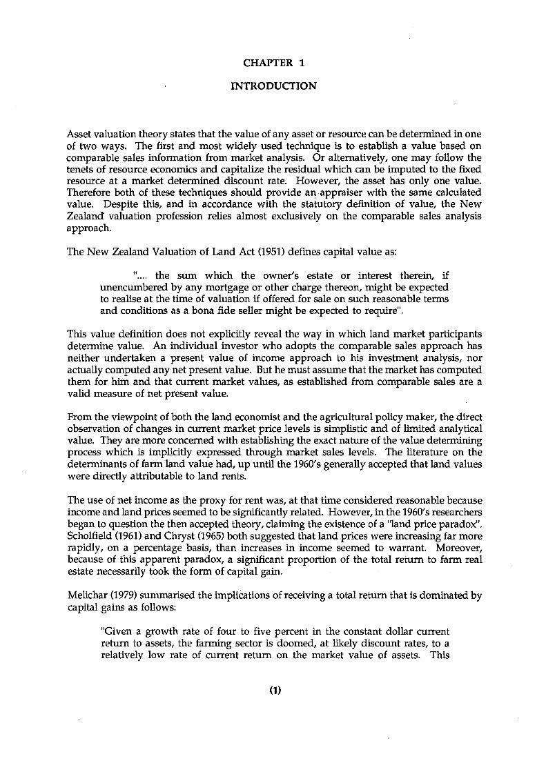
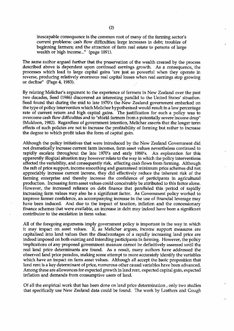
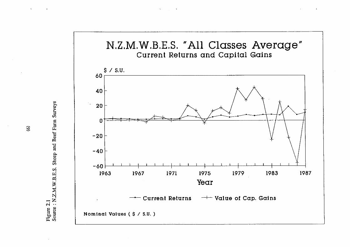
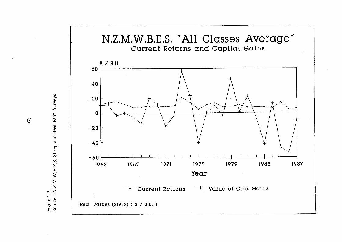
From 1962 to 1982, total production assets increased at an average annual compound rate of12.57 percent. Over the same twenty year period net income increased at only 9.33 percentin nominal terms. This apparent divergence between farm incomes and value is also evidentbetween 1972 and 1982 when the value of total production assets increased at an average rateof 20.35 percent per annum compared to an increase of just 13.42 percent for net income. Anexamination of the compound growth rates in real terms further accentuates what Scholfield(1961) and Chryst (1965) termed the "land price paradox", where land prices appeared to beincreasing more rapidly than increases in income seemed to warrant. From 1972 to 1982 thereal value of total production assets increased at a compound rate of 5.71 percent each yeareven though the real value of net farm incomes actually decreased by 0.37 percent perannum. This situation is shown graphically in figures 2.1 and 2.2 where current returns arecompared to the annual changes in the value of total production assets in both nominal andreal terms.

Many alternative theories have been advanced as an explanation for the divergence betweenfarm incomes and values, and these are subsequently examined in Chapter 3. But it may bepertinent to note that although nominal farm values continued to increase for the majorityof the 1962 - 1987 period, a significant decrease in values was experienced during the last fiveyears of the period. In fact, between 1982 and 1987 when real net incomes decreased at anannual compound rate of 5.37 percent, the real value of total production assets dropped bysome 18.86 percent per annum. It may therefore be reasonable to expect that those sameunknown factors which have caused farm values to increase at a disproportionately fast ratecompared to farm incomes may also operate in a reciprocal manner.

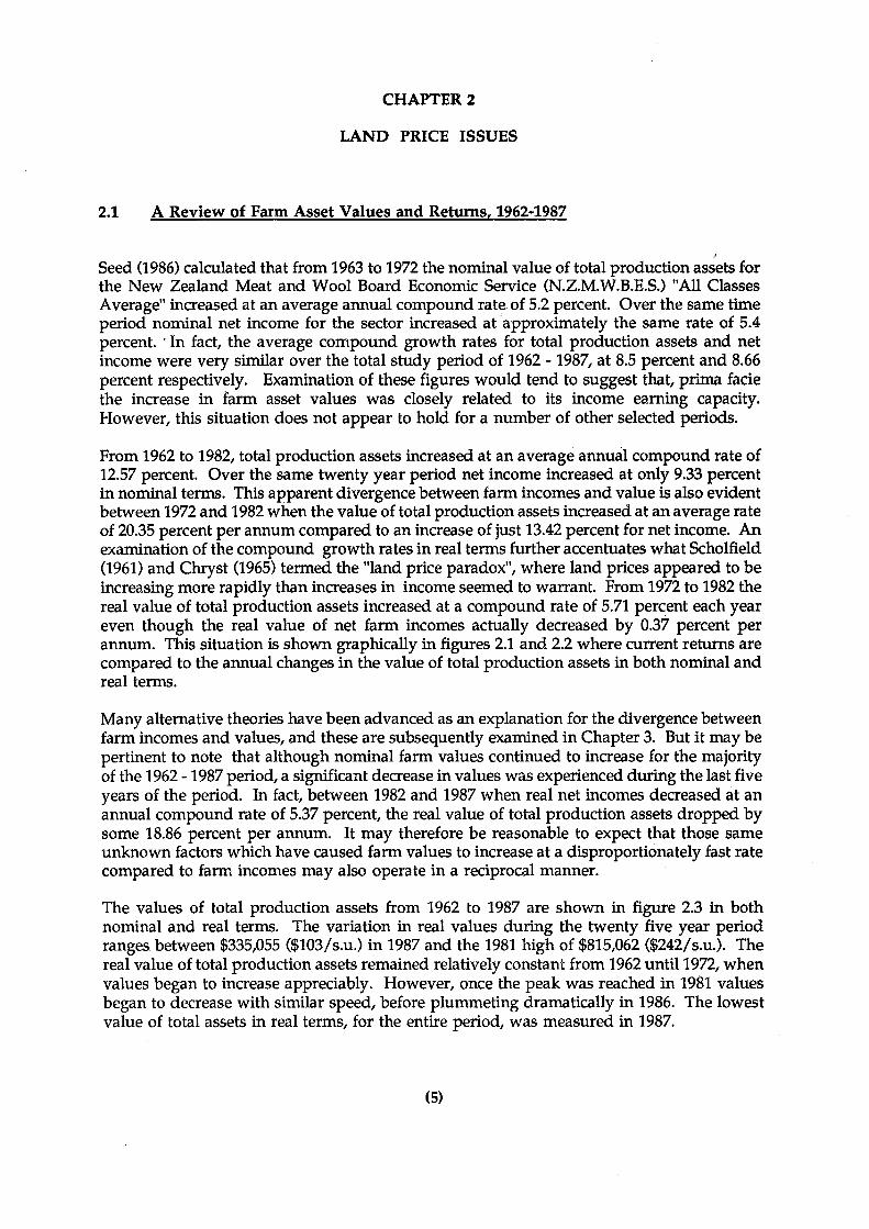
The values of total production assets from 1962 to 1987 are shown in figure 2.3 in bothnominal and real terms. The variation in real values during the twenty five year periodranges between $335,055 ($103/s.u.) in 1987 and the 1981 high of $815,062 ($242/s.u.). Thereal value of total production assets remained relatively constant from 1962 unti11972, whenvalues began to increase appreciably. However, once the peak was reached in 1981 valuesbegan to decrease with similar speed, before plummeting dramatically in 1986. The lowestvalue of total assets in real terms, for the entire period, was measured in 1987.

(5)

N.Z.M.W.B.E.S. II All Classes Average"Current Returns and Capital Gains

Nominal Values ( $ / S.U. )

----- Current Returns -+- Value of Cap. Gains

1987198319791975

Year19711967

20

$ / S.U.60r--------------------------,

40

- 60 f---JL..--L..--l.---t--J..-J..-.L.-..+--...l--...l--...l--+--...L--....L--....L---+--'---'------'------+---'-----'---'----j

1963

-40

-20

tI:l>..lI)

~rn

....-.. ~\0 ~'-'

4-<lI)lI)

a:l"'Cl§p.,lI)lI)

..r::::rnrn~a:l

~~N

-zC'i ..lI) lI)

~~..... 0~rn

N.Z.M.W.B.E.S. II All Classes Average"Current Returns and Capital Gains

1987198319791975

Year19711967

Ol--~-:;.k----I---\----+---\--_.¥__~>rl_---*---_\_-__I_+_--___l

--- Current Returns -+- Value of Cap. Gains

20

$ / S.U.60 r-----------;-----------------,

40

- 6 0 1---'-------'-------'------+---L...---'--...L-.-+---l---L.--L--+---'---'----'----+-~__'___'_____+_--'-----'-----'----1

1963

-40

-20

Real Values ($1982) ( $ / S.U. )

Vl>.CI)

~en

~ ~- ~~CI)CI)

~

'"Cla0..Il)Il).cenen~~

~:EN

NZN ..Il) Il)

~~..... 0~en

(8)

The variation of values in nominal tenns presents a rather different picture. Although thenominal value of total production assets still remained relatively constant until 1973, theescalation of fann values during the following ten year period is more accentuated than thatobserved in real terms. The value of nominal total production assets for the N.Z.M.W.B.E.S."All Classes Average" increased from $186,220 in 1973 to $789,041 at the end of 1982. Thisis a significant increase, and as explained earlier, one that does not appear to be closely orexclusively related to the associated increases in net fann incomes. Before examining thepossible causes of this apparent disparity between the growth in fann incomes and theincreases in fann asset values, it is important to examine the consequences of such large fannvalue fluctuations with particular reference to economic efficiency and equity. These factorsare addressed in the following Section. '

2.2 Factors Affecting Farm Asset Value Fluctuations

Melichar (1979) has asserted that any government action which attempts to support oraugment fann income does not increase the profitability of fanning but instead increases thedegree to which profit takes the fonn of capital gains rather than current return. As Section4.5 below explains, the New Zealand government has introduced many policy initiatives overthe 1962 .. 1987 period which were designed precisely for this purpose. For example, LeHeron (1989) observes that such policies as the Livestock Improvement Scheme and LandDevelopment Encouragement Loans were introduced during the late 1970's to stimulatefurther investment in pastoral agriculture. However, the author suggests that if these policieswere to be successful, the government also needed to provide fanners with some assurancethat future product prices would not suffer a substantial decrease. A SupplementaryMinimum Price Scheme was therefore introduced in an attempt to ensure fann incomesremained at an adequate level.

If Melichar's argument is accepted, the major consequence of the Government's incomesupport scheme during the late 1970's and early 1980's was to amplify the increases in fannasset values which occurred over that period. In a later paper Melichar (1983) suggests thatthe preservation of the wealth created by the process described above is dependent uponcontinued earnings growth. When real earnings stop growing or decline, relatively large realcapital losses may result as the processes which create the large capital gains are just aspowerful when they operate in reverse. The implications of this argument may certainly beconstrued as being analogous to the experience of New Zealand fanners since 1984. Theelection of a Labour government in 1984 saw virtually all existing agricultural supportmeasures being either immediately removed or phased out over a period of time and, withthe exception of 1985, coincided with a significant decrease in real net fann incomes. Thatlarge real capital losses were subsequently experienced during the 1984 - 1987 period couldbe due, at least in part, to the processes to which Melichar was referring.

The preceding discussion suggests that a number of additional economic adjustments followany government attempt to subsidize or maintain farm incomes. First, if policy makers wishto sustain fann incomes at an 'adequate' level, for whatever reason, then it should beacknowledged that these policies may have a greater impact on asset prices than on currentfarm cash flows. Although a wealth increment may be effectively conferred on existing landowners, their cash incomes may not necessarily be enhanced. Seed (1986) points out that theoutcome of the policy may in fact be immiserising rather than beneficial to the group thepolicy is targeted at.

N.Z.M.W.B.E.S. "AII Classes Average"Total Production Assets

19871982197719721967

O\--~~~L_jc______l--.l-----l.-----l.___+-----l.----.l..---.L---.L_+__--L--L--L--.L_+_-...L--...L--...L--...L-_____j

1962

Year

---- Nominal Values -t- Real (1982) Values

50

100

200

150

250

( $ / S.U. )300r--------------------------,

Real (1982) and Nominal Values

<n:>..4)

~en

...-. ~0' l:L4- 4-<4)4)

~

"d§0..4)4)

.r::CI)

en~~

~::E~

MZN ..4) 4)

t1~..... 0l:L4en

(10)

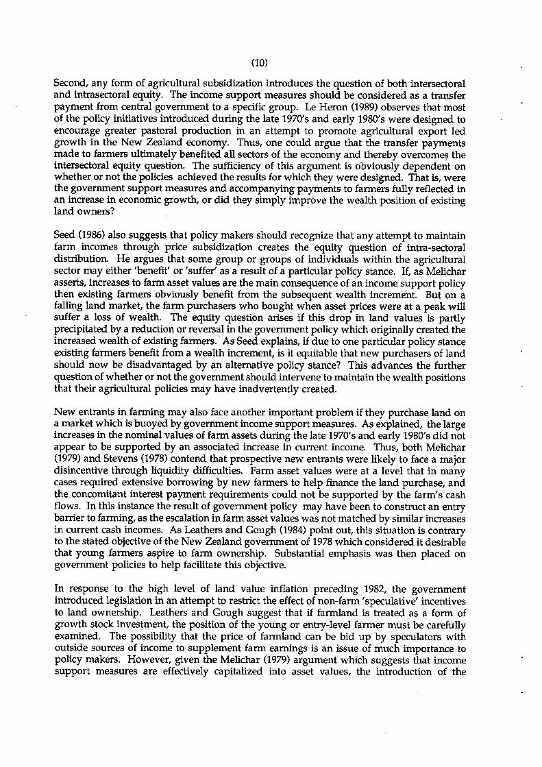
Second, any form of agricultural subsidization introduces the question of both intersectoraland intrasectoral equity. The income support measures should be considered as a transferpayment from central government to a specific group. Le Heron (1989) observes that mostof the policy initiatives introduced during the late 1970's and early 1980's were designed toencourage greater pastoral production in an attempt to promote agricultural export ledgrowth in the New Zealand economy. Thus, one could argue that the transfer paymentsmade to farmers ultimately benefited all sectors of the economy and thereby overcome~ theintersectoral equity question. The sufficiency of this argument is obviously dependent onwhether or not the policies achieved the results for which they were designed. That is, werethe government support measures and accompanying payments to farmers fully reflected inan increase in economic growth, or did they simply improve the wealth position of existingland owners?

Seed (1986) also suggests that policy makers should recognize that any attempt to maintainfarm incomes through price subsidization creates the equity question of intra-sectoraldistribution. He argues that some group or groups of individuals within the agriculturalsector may either 'benefit' or'suffer' as a result of a particular policy stance. If, as Melicharasserts, increases to farm asset values are the main consequence of an income support policythen existing farmers obviously benefit from the subsequent wealth increment. But on afalling land market, the farm purchasers who bought when asset prices were at a peak willsuffer a loss of wealth. The equity question arises if this drop in land values is partlyprecipitated by a reduction or reversal in the government policy which originally created theincreased wealth of existing farmers. As Seed explains, if due to one particular policy stanceexisting farmers benefit from a wealth increment, is it equitable that new purchasers of landshould now be disadvantaged by an alternative policy stance? This advances the furtherquestion of whether or not the government should intervene to maintain the wealth positionsthat their agricultural policies may have inadvertently created.

New entrants in farming may also face another important problem if they purchase land ona market which is buoyed by government income support measures. As explained, the largeincreases in the nominal values of farm assets during the late 1970's and early 1980's did notappear to be supported by an associated increase in current income. Thus, both Melichar(1979) and Stevens (1978) contend that prospective new entrants were likely to face a majordisincentive through liquidity difficulties. Farm asset values were at a level that in manycases required extensive borrowing by new farmers to help finance the land purchase, andthe concomitant interest payment requirements could not be supported by the farm's cashflows. In this instance the result of government policy may have been to construct an entrybarrier to farming, as the escalation in farm asset values was not matched by similar increasesin current cash incomes. As Leathers and Gough (1984) point out, this situation is contraryto the stated objective of the New Zealand government of 1978 which considered it desirablethat young farmers aspire to farm ownership. Substantial emphasis was then placed ongovernment policies to help facilitate this objective.

In response to the high level of land value inflation preceding 1982, the governmentintroduced legislation in an attempt to restrict the effect of non-farm 'speculative' incentivesto land ownership. Leathers and Gough suggest that if farmland is treated as a form ofgrowth stock investment, the position of the young or entry-level farmer must be carefullyexamined. The possibility that the price of farmland can be bid up by speculators withoutside sources of income to supplement farm earnings is an issue of much importance topolicy makers. However, given the Melichar (1979) argument which suggests that incomesupport measures are effectively capitalized into asset values, the introduction of the

(11)

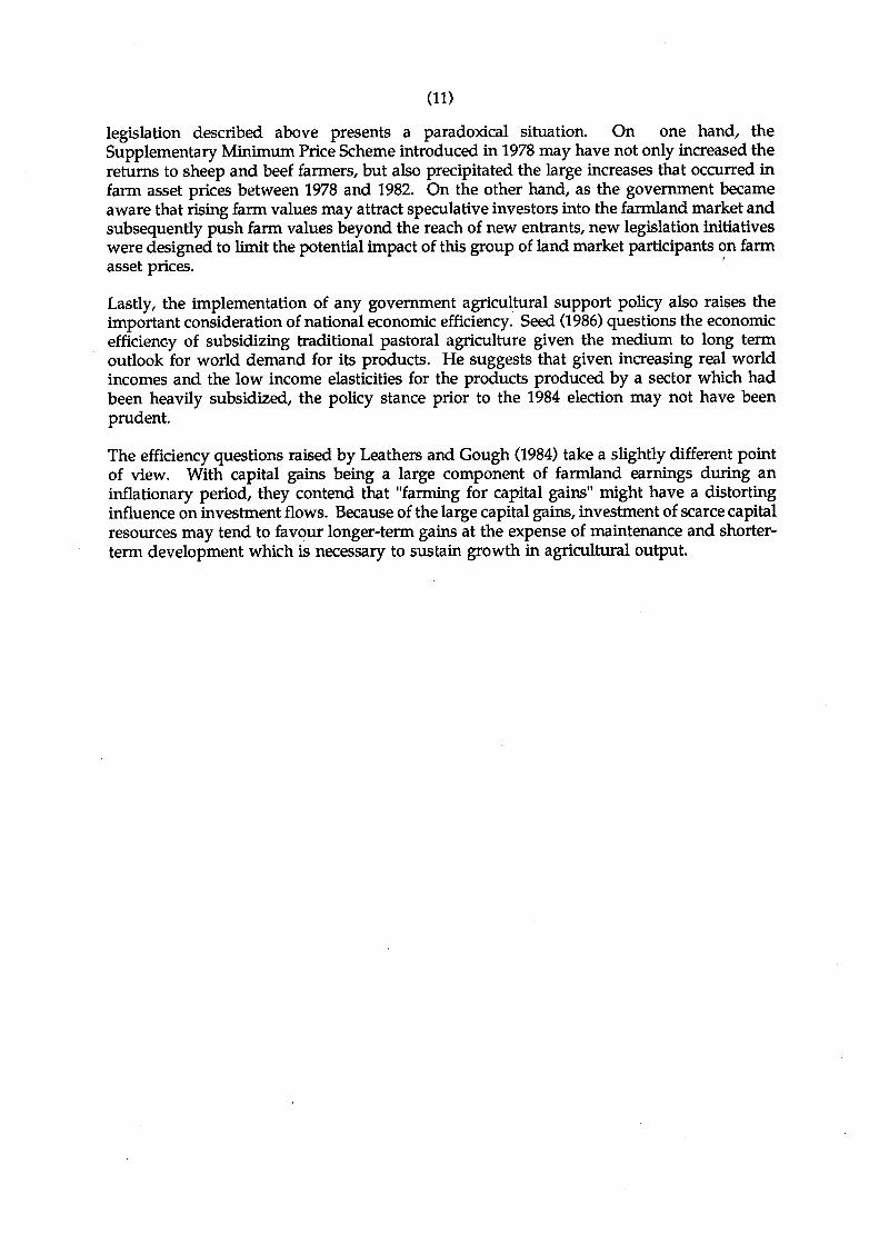
legislation described above presents a paradoxical situation. On one hand, theSupplementary Minimum Price Scheme introduced in 1978 may have not only increased thereturns to sheep and beef farmers, but also precipitated the large increases that occurred infarm asset prices between 1978 and 1982. On the other hand, as the government becameaware that rising farm values may attract speculative investors into the farmland market andsubsequently push·farm values beyond the reach of new entrants, new legislation initiativeswere designed to limit the potential impact of this group of land market participants on farmasset prices. '

Lastly, the implementation of any government agricu~tural support policy also raises theimportant consideration of national economic efficiency. Seed (1986) questions the economicefficiency of subsidizing traditional pastoral agriculture given the medium to long termoutlook for world demand for its products. He suggests that given increasing real worldincomes and the low income elasticities for the products produced by a sector which hadbeen heavily subsidized, the policy stance prior to the 1984 election may not have beenprudent.

The efficiency questions raised by Leathers and Gough (1984) take a slightly different pointof view. With capital gains being a large component of farmland earnings during aninflationary period, they contend that "farming for capital gains" might have a distortinginfluence on investment flows. Because of the large capital gains, investment of scarce capitalresources may tend to favour longer-term gains at the expense of maintenance and shorterterm development which is necessary to sustain growth in agricultural output.

CHAPTER 3

THE COMPETING THEORIES FOR LAND PRICE DETERMINATION

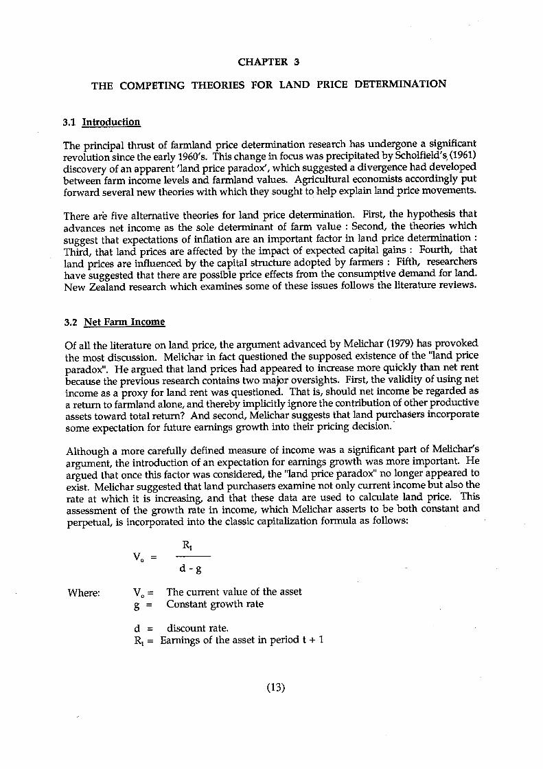
3.1 Introduction

The principal thrust of farmland price determination research has undergone a significantrevolution since the early 1960's. This change in focus was precipitated by Scholfield's, (1961)discovery of an apparent 'land price paradox', which suggested a divergence had developedbetween farm income levels and farmland values. Agricultural economists accordingly putforward several new theories with which they sought to help explain land price movements.

There are five alternative theories for land price determination. First, the hypothesis thatadvances net income as the sole determinant of farm value: Second, the theories whichsuggest that expectations of inflation are an important factor in land price determination :Third, that land prices are affected by the impact of expected capital gains: Fourth, thatland prices are influenced by the capital structure adopted by farmers: Fifth, researchershave suggested that there are possible price effects from the consumptive demand for land.New Zealand research which examines some of these issues follows the literature reviews.

3.2 Net Farm Income

Of all the literature on land price, the argument advanced by Melichar (1979) has provokedthe most discussion. Melichar in fact questioned the supposed existence of the "land priceparadox". He argued that land prices had appeared to increase more quickly than net rentbecause the previous research contains two major oversights. First, the validity of using netincome as a proxy for land rent was questioned. That is, should net income be regarded asa return to farmland alone, and thereby implicitly ignore the contribution of other productiveassets toward total return? And second, Melichar suggests that land purchasers incorporatesome expectation for future earnings growth into their pricing decision..

Although a more carefully defined measure of income was a significant part of Melichar'sargument, the introduction of an expectation for earnings growth was more important. Heargued that once this factor was considered, the "land price paradox" no longer appeared toexist. Melichar suggested that land purchasers examine not only current income but also therate at which it is increasing, and that these data are used to calculate land price. Thisassessment of the growth rate in income, which Melichar asserts to be both constant andperpetual, is incorporated into the classic capitalization formula as follows:

d-g

Where: The current value of the assetConstant growth rate

d = discount rate.R1 = Earnings of the asset in period t + 1

(13)

(14)

The author demonstrates that this formulation can generate an increase in land value in twoways. First, a change in R, g or d will result in a new value of Vo' And second, even if allof the variables are unchanged, land value will be increased as the expected return ismagnified by the constant growth rate.

Although the introduction of an income growth variable was largely supported by Reinseland Reinsel (1979) and Harris (1979), Melichar's assertion that expectations for income grqwthare constant and perpetual won less support. Reinsel and Reinsel concur that land earningshave not remained constant over time but have increased, invalidating the assumptions ofthe simplified capitalization model. However, following a, review of the trends in the ratioof cash rents to land value data for selected regions of the United States, they propose thatearnings expectations among land buyers have changed over time. This finding could alsohave an intuitive application to the New Zealand experience of the past two decades. Giventhe large historical fluc~tions in farming returns that have been observed since the 1960's,it is unlikely that participants in the farm land market have had a constant anticipation offuture earnings growth. Indeed, their experience of large income fluctuations throughout the1980's would have caused a continual reappraisal of farmers' expectations for future earnings.

In a review of the Melichar hypothesis, Doll and Widdows (1981) questioned whetherearnings growth has had the full effect suggested by the author. They agree with theconclusion that the growth in earnings has an effect on asset values, however, it is the extentof the effect that they question. Bergland and Randall (1984) supported Melichar's reasoningeven though they found evidence in the United States has shown that there has been a lessthan perfect correlation between rents and land price. Their research attempted todemonstrate that a one-off increase in land price can be generated by virtually any positivechange in expectations. The expectations of the participants in the land market may thereforebe important, even if Melichar's assumptions are overly simplistic.

Since these partial rejections of the constant income growth hypothesis, a raft of otherpossible price determinants have been suggested. However, Burt (1986) has also refuted thesupposed pricing influence of all these alternative factors, and again attempted todemonstrate the dominant role of land rents in the determination of farm prices.

Burt firstly argued that many of the recent land price studies have a common weakness intheir modelling approach. He concurs that rent expectations of buyers and sellers in thefarmland market are not the only influence on price levels, as "one would also expect adynamic adjustment mechanism in the movement of price between equilibria after someperturbation in the economy" (p. 12). But Burt then argues that one would have to be quiteoptimistic to anticipate identification of separate structures for price expectations andadjustment rigidities in the price of farmland. Models that have attempted to do so wouldnot be rejected statistically as time series data typically do not contain enough informationto reject any reasonable hypothesis.

The dynamic regression equation was estimated using net rent data from high quality grainland in illinois for the period of 1960 - 1983. The results show that the dynamic structure offarmland prices can indeed by quantified with a good deal of precision by a second-orderrational distributed lag on land rents. But the value, or ability of this model to explicitlyreveal the actual determinants of land price are not so clear and precise.

It must be assumed that the estimated equation is an approximation to a market adjustmentprocess, which is a weighted sum of both current rent, and rent from the previous period.

(15)

And further, it is assumed that these two rent figures comprise all the information utilizedby individual decision agents to estimate future rent. By his own admission, Burt recognizesthese assumptions to be very tenuous. If rental expectations are formulated using thiseconometrically derived structure, it implies they possess a very high level of economicsophistication. The interpretation of the results from this analysis also depend on the validitygiven to the above assumptions.

3.3 Expectations of Inflation

Much of the land price research has used a partial analysis strategy when attempting todetermine the causes of land price variation. That is, it has concentrated on the impact ofeconomic factors which are specific to agricultural production alone. Feldstein (1980a, 1980b)however adopted a general equilibrium framework in his attempt to discover thedeterminants of farmland value. He developed a model of portfolio equilibrium that notonly dealt with factors that influenced the price of land but also the impact of these factorson other assets that may be part of a rational investor's portfolio.

Feldstein proposed that the effect of inflation on asset returns in the United States is notneutral because of the tax system, where capital gains tax is lower than that for currentincome. The portfolio modeled in his study consists of three assets; land, bonds and shares,the last two Feldstein termed reproducible capital. Price equations were developed for eachasset, and the initial weighting of each holding related to a previous set of expectations aboutasset yields and risk. The current level of inflation is assumed to be known but the inflationrate for future time periods is not. The returns for all three assets are assumed to consist oftwo components. First, a real rate of return and second, an allowance for inflation gainswhich in the case of farmland is received through an increase in land value. Feldstein alsoargued that competition between investors will cause the ratio of the net marginal productsto asset price for each asset to be equal.

As the investor's expectation of inflation increases, the inflation component of the return foreach asset also increases. But Feldstein (1980b) pointed out that capital gains from land dueto inflation are taxed at a lower rate than income from other sources. Also, the payment oftax is deferred until the gain is realized. In contrast, the inflationary component of theinterest return from bonds, and the dividend return from shares are taxed at the ordinaryincome tax rate. Because the real rate of return to land is higher than that for the twoalternative asset classes, investors bid up the price of land to equate the marginal rates ofreturn between the assets of the portfolio.

Feldstein therefore suggests that the continuous increase in the price of land during the1970's in the United States may be considered to be a combination of two factors. Theequilibrium real price of land has changed as expectations of the inflation rate change. Andthe nominal price of land has increased continually at the historic rate of general inflation.

A number of researchers attempted to empirically test these assertions by specifying a modelthat included expected inflation as an explanatory variable. The study by Martin and Heady(1982) suggested that the expected rate of inflation, which was adaptively formulated, hasa negative impact on farmland prices. Alston (1985) also found that the inflation effect onland prices was significantly negative, although empirically small. The results of both ofthese tests would therefore indicate that the Feldstein hypothesis does not explain themovements in land price that it purported to. Further, Seed (1986) proposed that both the

(16)

work by Martin and Heady, and Alston tends to reinforce the Melichar hypothesis, thatgrowth in land prices is best explained by growth in net rentals.

That the empirical evidence does contradict the Feldstein theory may be explained by somereservations that Martin and Heady raised concerning the applicability of this theoreticalconstruct to the farmland market. They advanced two factors that could inhibit thehypothesised impact of inflation on real land prices. First, the land and financial <jlssetmarkets may not be adequately interrelated, thereby restricting the portfolio adjustmentprocess. And second, imperfect information may limit all investors' knowledge of futureinflation and tax rates.

The first of these cautionary points is most important. The degree to which the markets areinterrelated is thought to depend on the particular land market that is being addressed.Investors in farm real estc~.te may have extremely diverse reasons for purchasing land. Theymay be motivated to acquire a holding for its productive potential, its consumptive use, asa speculative investment, or to form part of a diversified asset portfolio. And the amountof consideration that each of these land users give to the returns available in other assetmarkets is also expected to differ appreciably.

The Feldstein portfolio adjustment process assumes that all prospective land buyers base theirdecision to purchase, at least in part, on the returns available from an investment in bothbonds and equity. And this further implies that the analyzed landmarket is dominated bybuyers whose primary interest in farmland is as part of a well diversified asset portfolio.

This may be a tenuous assumption to make in many cases. It is possible that the marginalland purchaser has quite different reasons for buying a property. If for example, farmlandprice is being set by consumptive users within a particular market, it is unlikely thatprospective returns from alternative investments are considered in the purchasing decision.As such, the hypothesised impact of inflationary expectations is reliant on a set of strictassumptions concerning the circumstances of land market participants. That the empiricalevidence of both Martin and Heady, and Alston rejected Feldstein's hypothesis may suggestthat the above assumptions are not met in reality.

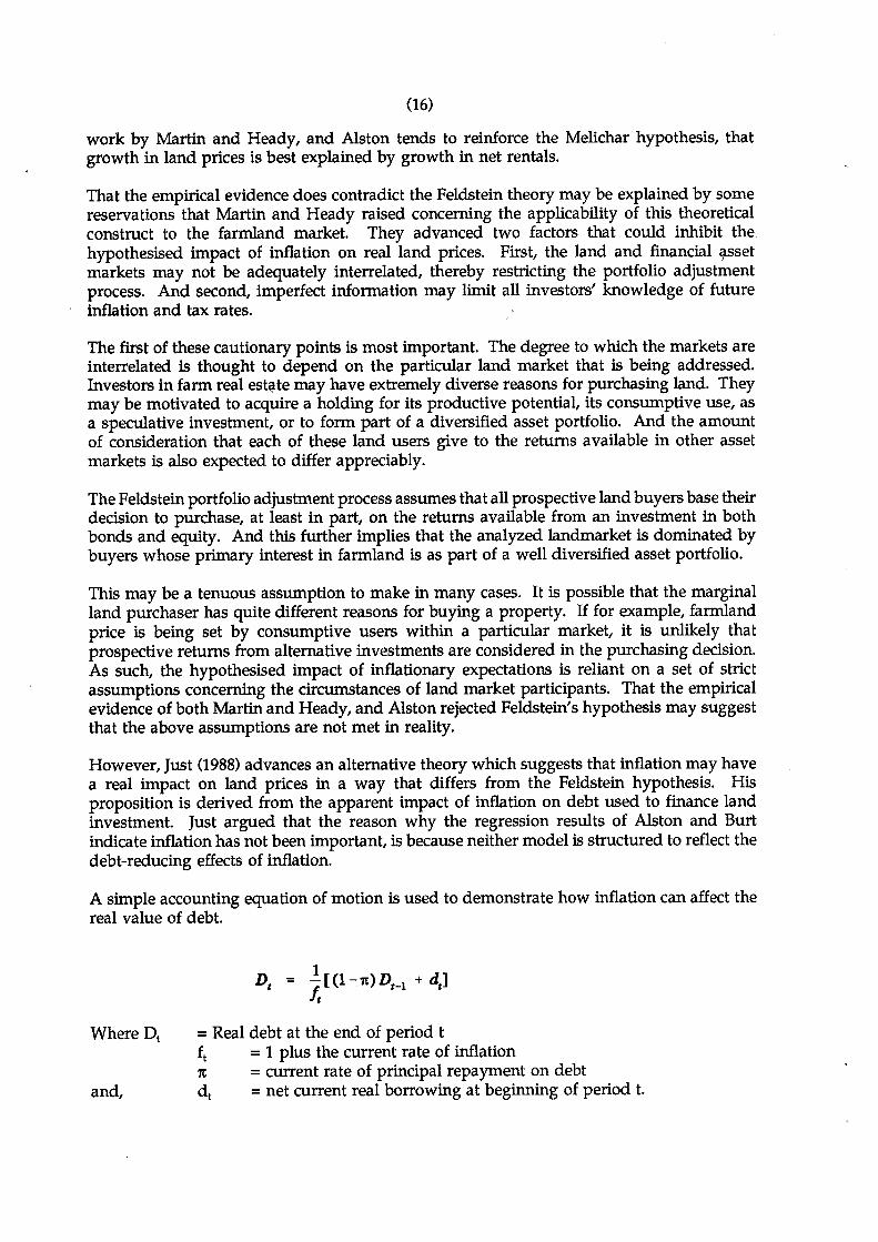
However, Just (1988) advances an alternative theory which suggests that inflation may havea real impact on land prices in a way that differs from the Feldstein hypothesis. Hisproposition is derived from the apparent impact of inflation on debt used to finance landinvestment. Just argued that the reason why the regression results of Alston and Burtindicate inflation has not been important, is because neither model is structured to reflect thedebt-reducing effects of inflation.

A simple accounting equation of motion is used to demonstrate how inflation can affect thereal value of debt.

Where Dt

and,

= Real debt at the end of period tft = 1 plus the current rate of inflation1t =current rate of principal repayment on debtdt = net current real borrowing at beginning of period t.

(17)

Just suggests that this equation reflects the rapid rate of real debt retirement that a farmercan expect with high inflation even allowing for relatively small payments of principal.Conversely, this debt-reducing advantage of holding land is lost in a period of low inflation.If the real value of debt is being eroded then landowner wealth must be improved, assumingasset values are at least being maintained in real terms.

3.4 Expectations of Capital Gains

Observations of large increases in farmland value during the 1970's has led a number ofeconomists to suggest that an expectation of capital gains is itself an important explanatoryvariable'of the price movements. The aggregate levels of capital gains in the United Stateshave been very large. Bhatia (1972) estimated that between 1947 and 1968 real capital gainson farm real estate in that country amounted to U.S. $87.9 billion. The subsequent figure forthe 1970's is also expected to be as significant. Melichar (1979) added that in the UnitedStates, annual increases in asset values had exceeded annual income by wide margins.Because of the significance of capital gains, some researchers reasoned that intending landmarket participants must incorporate some expectation of future capital gains into theirpricing decisions. The reasons that they give for doing so are however not necessarily thesame, and in some cases a capital gain variable is included with no apparent theoreticaljustification. Instead, the main focus of the capital gains literature concerns the way in whichland owners are hypothesised to value the expected increases in the price of their land.

Bhatia (1972) proposed that capital gains do not have to be realised to supplement currentincome, as the land owner has two alternatives. He can reduce his level of savings now inanticipation of receiving the expected capital gain when the property is sold. Or he mayborrow against the security of the appreciated value of the asset. It is argued that either ofthese alternatives will allow the farmer to benefit from increased land values before sellinghis farm.

Bhatia does not however suggest any explanation for the reasons why landmarketparticipants should include expected capital gains in their determination of land price. Itmust be assumed that it is included solely because capital gains have been observed in thepast. And for no other reason than this, land purchasers should expect the appreciation ofvalues to continue.

Plaxico (1979) does however offer an explanation for the inclusion of the capital gainsvariable. He argues that land can in some cases be likened to nonproductive assets such asgold, diamonds and artwork. This form of asset does not generate current income orproduce a cash-flow, but rather acts as a repository for value storage and preservation.Plaxico suggests that the speculative forces which prevail in the market for these assets alsohas an influence in the land market. The productive potential of the land may therefore beof secondary importance as investors purchase a property with possible future priceappreciation as their major consideration. This assertion relies to a great extent upon anyassumptions made about the marginal land purchaser, and the particular land market beinganalyzed.

The relative importance of speculative forces has been statistically evaluated by enteringboth net returns and capital gains into a regression equation purported to explain land prices.However, Burt (1986) states that interpretation of the given results is extremely difficultbecause of the way the model is usually specified. An examination of the Plaxico theory is

(18)

even more difficult. Even if the estimated parameter for expected capital gain is significantlydifferent from zero, one is unable to explicitly identify the reasons for its importance.

The study by Plaxico and Khetke (1979) again concentrated on the way that land purchasersvalue expected capital gain. In an extension of the work done by Bhatia, they also reiteratedthe argument that capital gains do not have to be realised to be spent. As the value of aproperty appreciates, the associated increases in the farmer's equity will either be availableas a financial reserve, or allow increased borrowing.

Three models were used to help examine the way market participants value expected capitalgains. The first suggested that the value of capital gains is the present value of theanticipated post-tax gain, which is received when the property is sold. Although Dunford(1980) supported this approach in his review of the Plaxico and Kletke study, the authorsargue that it fails to incorporate any benefit that an increase in equity may provide. Insteadthey recommend that the highest value of capital gains may be measured using the earningscapacity of newly borrowed capital, which is made available by the increase in equity. Thetwo further models were specified so that expected asset appreciation was valued in thisway.

However, Dunford argues that such an approach can only be used on a flow basis if theadditional borrowing power is used annually and as soon as it becomes available. Seed(1986) then suggests that the reality of liquidity problems in the short term may reduce thevalue of expected capital gains. New farmers may be unable to utilise the increasing debtcapacity because of their inability to meet the servicing requirements. .

Another method of valuing expected capital gains is given by Castle and Hoch (1982). Theysuggest that the divergence between land rents and prices can be explained if annualincreases in land price are included as current income. Castle and Hoch propose that theprice of real estate is determined by three components. First, they maintain that the presentvalue of future earnings to land is an important determinant of land value. This is measuredby the capitalised value of the net rent from the land. The second component of value isderived from the expected rate of growth in the asset price. Importantly this growth isassumed to remain constant into perpetuity, and be regarded as a source of current income.Castle and H6ch further suggest that this 'return' from capital gains is capitalized into valuein the same way as net rents.

The final price determining factor is a consequence of possible inefficiencies in the financialmarket. This occurs when market interest rates do not fully account for inflation, therebyconferring an advantage to borrowers as the general price level increases. The real price ofland should therefore increase as the real rate of interest is lowered during periods ofinflation, assuming the investor uses debt to help finance the land purchase.

In a review of this theory, Bergland and Randall (1984) doubted that the expected capitalgains variable actually captures the impact on farmland price which it is intended to. Theyargue that what Castle and Hoch termed the "capitalization of capital gains" can just asreadily be explained as the capitalization of the growth in rents. As such Bergland andRandall effectively reassert that the Melichar (1979) constant income growth hypothesis is thetrue model of land price determination. The Melichar theory has already been discussed, andthe assumption that land prices and rents increase or decrease in concert has been largelydiscounted. As Seed (1986) points out, "in the United States at least, land rents levelled offin approximately 1974 while land prices continued to increase until the early 1980's" (p. 51).

(19)

Thus the role of capitalized asset appreciation in a model of land price determination remainsambiguous. It may also be argued that the theoretical justification for including capital gainas an explanatory variable for land value, in any form, seems obscure. If the definition ofcapital gain is taken to be the first difference in annual asset values, then the factors whichcontribute to this capital gain are likely to be included in the explanation for land pricechanges which this research attempts to identify. That is, the identity of other economic orfinancial variables which lead land market participants to form their expectations f9r landprice appreciation.

It is suggested that the authors who include expected capital gain as a variable are implicitlyaggregating some of the determinants which need to be identified. Indeed, in the study byCastle and Hoch (1982) the factors which were attributed to causing capital gain were blandlydescribed .as "factors specific to the agricultural sector". By including such a nondescriptexplanatory variable, the relative importance of each of these "specific factors" is concealed.

Nevertheless, despite the concerns over the limiting restrictions that are included in theirtheory, Castle and Hoch did describe a potentially important variable. The impact ofinflation on the real cost of borrowing, and the associated effect this variable may have onland price is of considerable interest. It is however only one factor which brings attentionto the possible importance of capital structure in the determination of farm asset values.

3.5 The Impact of Financial Leverage

Most farmland price literature concentrates on factors that may affect the economic returnsfrom the land. Impacts of such variables as current returns, the expected growth rate ofincome, inflation and the benefits of asset appreciation have been discussed above withrespect to the farmers' expected future income pattern. Although each of these econometricstudies must implicitly incorporate a discount rate with which to capitalize expected returns,little of the reviewed research has concentrated on the manner in which this discount rate isestablished.

Any capitalization rate used to derive asset value is in effect a summary figure that maysubsume several significant variables other than just the investor's rate of time preference.These include the land owner's risk aversion, taxation position and possibly moreimportantly, the level of debt used in his capital structure.

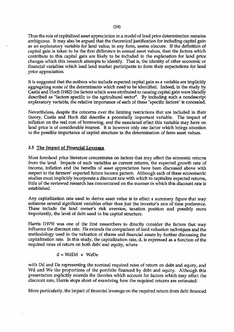
Harris (1979) was one of the first researchers to directly consider the factors that mayinfluence the discount rate. He extends the comparison of land valuation techniques and themethodology used in the valuation of shares and financial assets by further discussing thecapitalization rate. In this study, the capitalization rate, d, is expressed as a function of therequired rates of return on both debt and equity, where

d =WdDd + WeDe

with Dd and De representing the nominal required rates of return on debt and equity, andWd and We the proportions of the portfolio financed by debt and equity. Although thispresentation explicitly extends the theories which account for factors which may affect thediscount rate, Harris stops short of examining how the required returns are estimated.

More particularly, the impact of financial leverage on the required return from debt financed

(20)

assets was not discussed. The deductibility of interest payments from taxable income is avaluable advantage of using borrowed capital to fund asset purchases. And hecause of thistax generated advantage, the effective post-tax cost of debt is reduced. The associated costsof equity financed assets are not however deducted from income before the tax liability isassessed. As such, the overall cost of capital can be seen to be dependent on the ratio of debtto equity in the capital structure. The marginal tax rate in New Zealand has been as highas 67.5% during the 1962 - 1987 period, and this could have had a significant impact op therequired rate of return on debt used to purchase assets.

The proportions of debt and equity effected in the capi~al structure of the marginal landpurchaser, and the effective tax rate of the borrower will substantially influence the eventualcapitalization rate used in the determination of both the required return on invested equityandof the land price. As with any investment, if the required rate of return is reduced thenthe price an intending asset owner can afford to pay must increase. This is no less true forinvestment in farmland.

The taxation advantages of using debt finance in the farm purchase can also be added to, oramplified by a number of other factors. As described above, the marginal income tax ratesin New Zealand have been relatively high, and have therefore magnified the effect taxdeductibility can have on an investor's required rate of return.

Even if the impacts of taxation and debt erosion are disregarded, the required returns fromdebt and equity financed assets in New Zealand were unlikely to be the same dUring the pasttwenty five years. Numerous support measures were introduced by the New Zealandgovernment during the 1970's, one of which provided concessionary loans for investment inagriculture. Debt funding was therefore available for farm purchase at a cost that wasconsiderably below the market interest rate. This gave intending farmers a distinct incentiveto use debt finance, and effectively reduced their required rate of return and capitalizationrate.

3.6 Accounting for Consumptive Values

Several economists state that land is not only an input into agricultural production but alsoan important argument in many individuals utility functions. Land may not be purchasedsolely for its productive value but rather for consumptive use and enjoyment.

Both Pope and Goodwin (1984) and Pope (1985) therefore suggest that land price may beinfluenced by not only productive and speculative value, but also its consumptive value.This consumptive value is thought to depend on size, proximity to metropolitan areas andaesthetic or romantic appeal. Indeed, Pope states that consumptive users of rural land choosea farm in the same manner in which they would choose a hat; style may be of moreimportance than functional form.

Whether or not consumptive demand should be included as a possible land pricedeterminant depends largely upon the particular land market of interest. If it is to beincorporated into a model, one must assume that land value is being influenced by theseconsumptive users. Pope and Goodwin suggest that the relative importance of productiveand consumptive values alter with farm size. The smaller the parcel of land the higher theconsumptive use component. Or alternatively, as the size of the farm increases, the influenceof consumptive values on land price decreases as the productive use becomes more

(21)

important. The authors also point out that these smaller units are concentrated closer tometropolitan areas where they are more likely to have high recreational, aesthetic or romanticappeal.

Pope (1985) attempted to empirically test the theory of consumptive demand using a sampleof rural land in Texas. His model of the land market assumes that land value is determinedby both productive and consumptive values, while the demand for land by consu,mptiveusers is a function of income, taste, population density and the availability of substitutes.The results indicated that net returns to land explained less than one quarter of the marketvalue of land in Texas. Pope then concluded the consumptive demand for land wouldcontinue to apply strong upward pressures on rural hind values.

The main inference suggested by these conclusions is that the majority of farmlandpurchasers in Texas derive income from other, non-farm sources which can be used tosubsidise their particular choice of farming operation. The participants in this market areassumed to be purchasing a lifestyle and any income that the property earns is incidental.As Seed (1986) points out, these assumptions should be extrapolated to other land marketswith extreme care, and are probably not directly applicable to the majority of rural landmarkets in New Zealand.

3.7 New Zealand Research

Lee (1976) and Lee anp Rask (1976) developed and refined a "bid-price" model to evaluatefarmland prices, or more specifically to provide the land buyer with a method of determiningfarm value. Leathers and Gough (1984) replicated this modelling framework using NewZealand data. Using both New Zealand Meat and Wool Board Economic Service and NewZealand Valuation Department data Leathers and Gough attempted to identify the factorsor variables that influenced the land value of sheep and beef farms. They also attemptedto examine the impact of "inflationary and non inflationary economic conditions" on landvalues as well as identifying policy implications. But, as Seed (1986) points out, theusefulness of the "bid-price" approach for establishing land price determinants is limited:

"Unfortunately, the Lee and Rask model was not the most appropriate (tofulfil their objectives), as it is a non-parametric deterministic model. That is,there is no relationship estimated between the explanatory variables and thedependent variable (bid price), as well, uncertainty is not included. Mostimportantly however, how do we know that the Lee and Rask specificationbest describes the "true" model? Given that the variables have been selectedfrom theory, but are untested, what weight can be placed upon sensitivityanalysis when the significance of one variable over another is the result of it'smathematical specification? The model does produce estimates of the bidprice which closely approximate the land values at that time, although, givenit's structure this is hardly surprising" (p.28).

Considering these reservations, a further review of the research by Leathers and Gough islikely to be of limited value.

For the purposes of this study the models specified by Seed hold more interest as they areeach stochastic and parametric. And as such, they have the potential to more accuratelydetermine the influence any variable may have on land value. The author stated his study

(22)

objective was to:

"examine the determinants of the price of fattening and grazing farm land inNew Zealand over the period of 1962 to 1983. More particularly, (heexamined) the relationship between real land price and expectations of realincome, real capital gains and the rate of inflation for sheep and beef farms"(p.158).

Having examined the relevant theory and literature on the topic, Seed observed that threebroad themes emerged. He then specified a separate model to represent each of thesetheories, and empirically tested them to identify the one which best explains land pricemovements.

The first model attempteg to represent and test the theory advanced by Melichar (1979) and(1983). The central tenet of this theory is that land behaves as a growth stock. That is, it isassumed that the growth rates of both the value of the asset and its earnings are constant andequal in perpetuity. A second testable model was then specified to incorporate theargUments of Bhatia (1972), Plaxico and Kletke (1979) and Castle and Hoch (1982). Andfinally, the third model expressed farmland prices as a function of expected net rental incomeand the expected rate of inflation. This was based on the Feldstein (1980a) and (1980b)hypothesis where expectations of a change in inflation combined with the structure of theUnited States tax laws leads to changes in the real price of land. That is, the basic neutralityof taxes and inflation broke down when their simultaneous effects were considered.

All three models were estimated using a number of alternative techniques, with model twoproving to be superior to the others. That model produced the highest adjusted R-squared(0.7221) compared to the relevant versions of the other two. But given that this study'sobjective was to "examine the determinants of the price of fattening and grazing farm land"one may argue that the approach taken by Seed was not the most appropriate. All of thesemodels have been based on a mainly theoretical treatise, which by definition abstract awayfrom what may be expected to happen in reality. The theories of Melichar (1979), Castle andHoch (1982) and Feldstein (1980a) (1980b) do not purport to completely explain all land pricemovements, but are merely advanced as a contributory factor. Therefore, the ability of eachof Seed's models to identify land price determinants should be expected, a priori, to beinadequate. Nevertheless, Seed maintains that the adjusted R-squared (0.7221) represents a"reasonably good fit" and that "this model provides some evidence that increasing landvalues may be likened to the appreciation which occurs in the value of other assets such asgold or artwork". But, as has already been argued, estimating a significantly positiveexpected capital gain coefficient does not reveal the reasons for such expectations. Thejustification for claiming that some speculative motive has caused the observed capital gainis unclear. The expectations could as easily be based on several other variables which maybe incorporated into the land purchasers decision. These may include expected inflation andthe value increments from debt erosion, and expectation for changing taxation and interestrates, or an expectation for future earnings growth. By merely including an expected capitalgain variable in the model, a more precise examination for the causes of the expectationscannot be made. And therefore, even if the explanatory power of model two is consideredreasonable, it's ability to explicitly identify land price determinants is unsatisfactory.

Another major weakness of this study is considered to be the use of the New Zealand Meatand Wool Board Economic Service Survey (N.Z.M.W.B.E.S.) "All Classes Average" as theanalyzed sector. The time series data taken for asset value, net income and capital gain are

(23)

a weighted average of all seven farm classes surveyed by the N.Z.M.W.B.E.5.This approachimplicitly assumes that an aggregate New Zealand market exists for all sheep and beefgrazing land, and more importantly, that all grazing land has similar qualities. Assuminghomogeneity in this aggregate market is still important even if using per hectare data negatesthe effect of productivity differences between the seven farm classes.

Although the productive capacity of a farm has an obvious influence on its value, tl}ere areseveral other factors which may also significantly affect land price. These include the regionin which the property is located, the attractiveness of that regions' climate, the property'svicinity to towns and cities, and it's potential for more intensive development. And becausethese land qualities vary greatly between most farming regions, the aggregate marketassumption breaks down. The motives for purchasing farmland are expected to depend onthe region the farm is situated in, and the productive and consumptive qualities that regionpossesses. Based on the theory of alternative motives for farmland demand, it is apparentthat the land market used in any analysis should be as homogeneous as possible. A pricemodel may then be able to more precisely incorporate the determinants of land price whichare considered relevant to that individual market.

CHAPTER 4

FINANCIAL LEVERAGE AS ANALTERNATIVE DETERMINANT OF LAND PRICE

4.1 Introduction

The literature review given above in Chapter 3 outlined numerous alternative theories, whichall purported to have some influence on the determination of land price. Before one, or anycombination of these variables can be incorporated into a land price model a number ofimportant considerations should be addressed.

Both Po"pe et al. (1979) and Doll and Widdows (1982c) found that none of the theoreticalresearch has suggested a model specification which is most appropriate to the farmlandmarket. Seed (1986) reasoned that as a result, there has been a proliferation of ad hoc modelswhere variables are added in an effort to improve the overall fit of the model to the data.Johnston (1984) argues further that such data mining produces valueless results from whichlittle information can be taken.

The first requirement of this study was to define an appropriate market on which to base theanalysis. Pope (1985) argues that the land market should not be considered to behomogeneous in the aggregate. He suggests that it may be subdivided into severalsubcategories based on certain characteristics that are unique to buyers or sellers. Theimportance of defining the market to be examined before hypothesising which of thealternative theories are thought to be relevant is therefore emphasized. This is discussed inSection 4.2. The geographic region from which the data has been taken for the analysis isthen described, before the hypothesized determinants of land price are presented.

The most appropriate analytical procedure for this study is described in Section 4.3 beforeconsidering the treatment of expectations, and the definition of the variables involved.

4.2 Definition of the Market for Farmland

A market, as defined by Kotler (1986) consists of all those people with an actual or potentialinterest in a commodity, as well as the right resources for exchanging it. This is the broadestmarket definition possible as it relates to a complete generic commodity class, within whichthere exists many subcategories. The market for farmland can be similarly divided intoseveral submarkets.

Doll and Widdows (1982b) suggest that the market for land in the United States may besubdivided into three categories, distinguished by the different motives that participants ineach market hold for purchasing land. First, the market for commercial farming land. In thissubmarket the productive demand for land is most important, although consumptive demandand the demand for land as a store of wealth still have some influence.

The second market category is that for part-time farming and rural residences where theconsumptive demand for land is the major factor in the formulation of land values. Thisland may have little or no value resulting from its productive capacity, and it is suggestedthat the determinants of land price are not dissimilar to those in the market for private urban

(25)

(26)

dwellings. The final land submarket identified by Doll and Widdows results from nonagricultural, spatial demand. In this category, land use is changing from agricultural or ruralresidence to industrial, commercial or urban uses. The main determinant of the size of thismarket is considered to be dependent on population growth in metropolitan areas. Whena land use change is imminent, speculative demand increases with little regard given to theland's agricultural potential.

Although this segmentation is helpful, each of the three given land submarkets should notbe assumed to be totally homogeneous. Specifically, the commerciallandmarket in NewZealand can be seen to embody many areas of farmland which possess distinctly differentcharacteristics. As has been pointed out in the review of Seed's (1986) work, the motives forpurchasing' commercial farmland cannot be expected to remain totally consistent in anaggregate market. They are expected to depend on the region the farm is situated in, andthe productive and consumptive qualities that region possesses.

In his review of the research, Burt (1986) argues that many of the apparent difficulties of theexisting empirical work are exacerbated by using aggregate data to analyze land prices. Thiswill introduce the problems of extreme heterogeneity in land quality, non-agricultural valuesof farmland which are not reflected in current or historical rents, institutional variations overtime and space, and inaccurate estimates of both rents and land values caused by accountingproblems in the former and sampling problems in the latter.

Robison, Lins and VenKataraman (1985) also highlighted the importance of constructing aland price model with reference to the particular market under analysis. Their studyattempted to show that cash rents and the growth in rents, as well as demand from nonagricultural land users are the critical determinants of land value. However, the model wasapplied to data from twenty four states in the United States, and gave seemingly inconsistentresults. The authors therefore concluded that there may be considerable variation amongstates in the factors which most strongly influence the land market.

The findings of both Robison et aI, and Burt emphasize the need to identify and define ahomogeneous market before selecting possible price determinants. The land value modelmay then be able to more precisely incorporate the factors considered relevant to thatindividual market. Further, any justification for using a proposed farm value determinantmust be related to the market participants and their motives. Attempting to pre-determinewhich factors are relevant in an aggregate market is obviously more difficult.

4.3 The Chosen Market

Consistent time series data for farm incomes and prices in New Zealand are not readilyavailable. The only consistent data series which contains adequate income and priceinformation is that compiled by the New Zealand Meat and Wool Board Economic Service(N.Z.M.W.B.E.S.). Their sheep and beef farm surveys have been produced since the 1957/58season, providing reasonably detailed physical and financial information for eight farmlandclasses.

The class seven farm category has been selected as possibly the most homogeneous sample,and will be used in this analysis for a number of reasons. Despite the fact that thecategorization of all sample farms is based on both the type and intensity of farmingundertaken, the farms within each sample class are in some cases located in several different

(27)

provincial areas. Thus, although levels of production within each class should be directlycomparable, a number of other factors that influence land value may not be consistent acrossthe sample. Certainly the most obvious of these is the region in which the property islocated. The attractiveness of that region's climate, the property's vicinity to towns and cities,and its potential for more intensive development should all be expected to have some impacton land values. It is therefore suggested that using a sample in which the farms do not sharea reasonable proximity to each other may introduce some inaccuracies to the analysi?

The majority of the properties in the class seven sample are located in Southland. And thelocation factors which influence the overall desirability of each sample farm are expected tobe relatively consistent. Difficulties that may result from variations in these consumptivevalues ate therefore minimised by the choice of this sample class.

Unfortunately there is an apparent dearth of recorded information which may help toestablish the circumstances or possible motives for land purchase of the participants in theSouthland farmland market. However, the New Zealand Valuation Department has recordedsome information concerning the land purchaser that may provide some insight into thepossible price determinants in this market. A broad classification of farm buyers was startedin 1970 which separated all purchasers into five categories. For each transfer of farmlandwithin the Southland provincial area, the purchaser was described either as an existingfarmer, a new entrant to farming, a businessman, a government agency or some other party.

Based on these general classifications, some assumptions concerning the predominant motivefor purchasing farmland can be made. The number of Southland farms that have beenpurchased by businessmen since 1970 is considered to be fairly insignificant. Of all theproperties that are classified as economically viable, the percentage that have been boughtby businessmen ranged between zero percent in 1979 to 12.5 percent in 1985. Importantly,that proportion can be seen to be far more significant in many other provincial areas.

Assuming that the influence of non-farm demand on land values is small, it is argued thata number of advanced price determinants can be reasonably disregarded for this study. TheValuation Department information helps to reinforce the assertion that the class sevenfarmland area is predominantly made up of single family units which are purchased for theirproductive use. As such, the possible impact of demand from consumptive users isconsidered small. The limited number of farm purchases by businessmen may also suggestthat the motive of anticipated capital gains has had a negligible influence on pricedetermination. If businessmen had purchased a significant number of the farms that weresold in Southland, any specified land price model would have to incorporate bothconsumptive and speculative demand.

As a result, basing the analysis on the Southland market facilitates a more explicitexamination of the impact of financial leverage as a number of theoretical factors presumedto affect land price can be justifiably omitted. Although the omission of such factors isessentially a subjective choice and lacks conclusive data-based support, it has an advantageover strictly ad-hoc specifications which have little regard to the analyzed market or thepurchasing motives of its participants.

4.4 The Land Price Equation

As explained, land price researchers have offered many different theories in an effort to

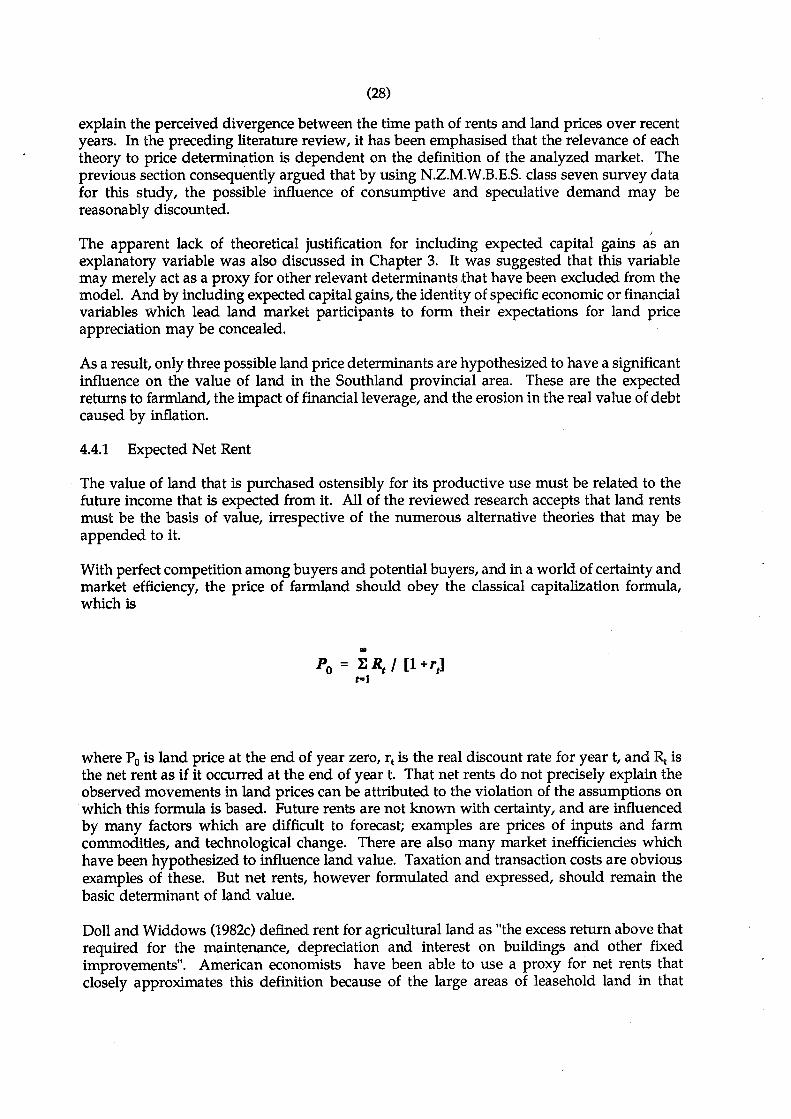
(28)

explain the perceived divergence between the time path of rents and land prices over recentyears. In the preceding literature review, it has been emphasised that the relevance of eachtheory to price determination is dependent on the definition of the analyzed market. Theprevious section consequently argued that by using N.Z.M.W.B.E.S. class seven survey datafor this study, the possible influence of consumptive and speculative demand may bereasonably discounted.

I

The apparent lack of theoretical justification for including expected capital gains as anexplanatory variable was also discussed in Chapter 3. It was suggested that this variablemay merely act as a proxy for other relevant determinants .that have been excluded from themodel. And by including expected capital gains, the identity of specific economic or financialvariables which lead land market participants to form their expectations for land priceappreciation may be concealed.

As a result, only three possible land price determinants are hypothesized to have a significantinfluence on the value of land in the Southland provincial area. These are the expectedreturns to farmland, the impact of financial leverage, and the erosion in the real value of debtcaused by inflation.

4.4.1 Expected Net Rent

The value of land that is purchased ostensibly for its productive use must be related to thefuture income that is expected from it. All of the reviewed research accepts that land rentsmust be the basis of value, irrespective of the numerous alternative theories that may beappended to it.

With perfect competition among buyers and potential buyers, and in a world of certainty andmarket efficiency, the price of farmland should obey the classical capitalization formula,which is

...Po = ERe I [l +7t]

t=1

where Po is land price at the end of year zero, rt is the real discount rate for year t, and ~ isthe net rent as if it occurred at the end of year t. That net rents do not precisely explain theobserved movements in land prices can be attributed to the violation of the assumptions onwhich this formula is based. Future rents are not known with certainty, and are influencedby many factors which are difficult to forecast; examples are prices of inputs and farmcommodities, and technological change. There are also many market inefficiencies whichhave been hypothesized to influence land value. Taxation and transaction costs are obviousexamples of these. But net rents, however formulated and expressed, should remain thebasic determinant of land value.

Doll and Widdows (1982c) defined rent for agricultural land as "the excess return above thatrequired for the maintenance, depreciation and interest on buildings and other fixedimprovements". American economists have been able to use a proxy for net rents thatclosely approximates this definition because of the large areas of leasehold land in that

(29)

country. The value of lease payments data also has an advantage of essentially representingthe value of expected net rents, as payments are usually made at the beginning of the leaseperiod. Landowners can therefore know with some certainty the returns they will achievefor the coming year, at the start of that year.

Land price researchers in New Zealand are unfortunately not afforded the same opportunity.The net farm income data provided by the N.Z.M.W.B.E.S. is not directly synonymous withnet rents and several adjustments need to be made. The adjusted data series does howeverprovide a reasonable proxy for rents. The procedure used is described in Section 4.7.2.

The incorporation of expectations into a land price model is more difficult. Withexpectations, land value is not assumed to depend on the actual value of net rent but ratheron the expected, or permanent future level of returns to land. Unfortunately, the way inwhich land market participants form these expectations is not known. That they aresubjective, and as such the personal judgements of an individual further compounds theproblem. Several econometric schemes can be used to represent the expectations formulationprocess, all of which are restricted to the use of historical rent data to help predict futurelevels. Although the ability of each scheme to closely represent the actual, but unknownmethod of producing expectations can be empirically measured, this 'artificial' estimationshould be expected to introduce some form of bias into the analysis. This important problemis further discussed in Section 4.6 before an expectations hypothesis is chosen for this study.

Despite the problems of definition and the formulation of a suitable expectations scheme, netrent is not surprisingly advanced as the major determinant of land price in the Southlandarea. However, this model will differ from the classical capitalization formula because of theway in which the discount rate is estimated, where the effects of both financial leverage anddebt erosion can be seen to magnify the apparent value of future rents.

4.4.2 The Impact of Financial Leverage

The theoretical justification for expecting financial leverage to have a significant impact onland value is rational and can be explained as follows. From the simple capitalizationformula, recall that value can be computed by capitalizing a residual to land, at anappropriate discount rate, or;

Po = Ali

where Po is the imputed asset value, A represents the expected constant annuity from landand i is the capitalization rate.

The impact of the choice of discount rate, or required rate of return on the computed assetprice is quite clear. Any change in the capitalization rate will have an effect on the imputedvalue. The capitalized effect of any proportional change in the discount rate increases as thediscount rate falls. Therefore, the accuracy with which this simple model can identify truemarket values is reliant on an accurate assessment of the marginal land purchasers' discountrate.

The discount rate used should describe the rate of return that a marginal land purchaserrequires from the invested funds. If the entire purchase price is funded from equity, thenthe appropriate discount rate is the investors' opportunity cost of capital. That rate should

(30)

equal the return available from his next best alternative investment which has both a similarrisk and temporal structure. However, when debt finance is introduced into the landpurchaser's capital structure it is argued that the appropriate discount rate then becomes anaverage of the two required rates of return weighted by the proportions of debt and equitycapital. Even if the impact of taxation is disregarded, the required returns from debt andequity financed assets is unlikely to be the same, and the weighted average cost of capitalwill differ from that for an all equity financed property.

Thus, if some proportion of the asset price is funded by debt finance the appropriatecapitalization rate, (~) is:

~ =(E/A" Ke) + (D/A" Kd)

Where: ~ = The weighted average cost of capital.

E/A = The proportion of assets financed by equity funds.

D/A = The proportion of assets financed by debt funds.

Ke = The post-tax required return on, (or cost of) equity funds.

Kd = The post-tax required return on, (or cost of) debt funds.

A commonly used proxy for the required return on equity capital has already been describedas the available return from some other risk eqUivalent investment.

However, the impact of a number of variables including risk must be contemplated beforethe effective cost of debt can be estimated. The deductibility of interest payments fromtaxable income is the most obvious advantage of using borrowed capital. This taxationadvantage reduces the effective cost of servicing the debt according to the marginal tax rateaffecting the relevant net profits. With a marginal income tax rate as high as 67.5% duringthe past twenty five years, each dollar spent on debt servicing had the potential to reducethe taxation payments by 67.5 cents.

Nevertheless, the degree to which these imputed advantages of financial leverage actuallyimpact on market land values depends ultimately upon the assumptions made about themarginal land purchaser. Or more precisely, what level of marginal tax does the marginalfarm buyer expect to pay? The degree to which the effective cost of debt is reduced dependsupon the size of the taxation saving which interest deductibility affords. The marginal taxrate paid by the marginal land purchaser is unfortunately not observable, and the procedureused in this study is restricted by that problem. However, for the purposes of this discussionwe can presume that both the taxation and capital structure position of the marginal landpurchaser are known, and then examine the consequences of relaxing this assumption inSection 4.5.

The capitalization rate has now been explicitly expressed as some function of the requiredreturns from both debt and equity funds. Introducing taxation produces a capitalization rate,Kt, which is calculated as;

(31)

~ = (E/A" I<e) + [0/A .. (~ (1 - T»]

where T represents the investor's marginal tax rate and all other variables as previouslydefined. Assuming a marginal tax rate greater than zero, the introduction of taxation can beseen to reduce the overall required rate of return, and consequently increase the capitalizedvalue of any given annuity.

This aggregated capitalization rate, or weighted average cost of capital cannot however beused to directly compute asset value. The respective returns to assets financed by either debtor equity funds are not subjected to the same taxation. treatment. Farm drawings are themain source of return to equity funds, but importantly this return must be subjected toincome taxation before becoming available. On the other hand, interest payments whichrepresent a return to debt financed assets are not taxed. If total net rents are capitalized bythe weighted average cost of capital, this differential tax treatment is not allowed for.

As a result, the aggregate expected annuity should be partitioned to represent a separatereturn for both debt and equity funds. The separate returns should be apportioned withrespect to the debt/asset ratio used by the land purchaser, and subsequently capitalized bythe relevant discount rate. Allowing for the differential tax treatment of returns to debt andequity, the appropriate capitalization formula then becomes;

v~ =[(1 - T) (E/A" YAE)]

d+

O/AxYAE

Mi(l - T)

where: V~ =d =~ =YAE =

The asset value, as at the beginning of the income year, tThe appropriate post-tax opportunity cost of equity fundsMortgage interest rateThe expected net profit to the asset.

with all other variables as previously defined.

Although this presentation does not introduce any more variables into the capitalizationformula, it does explicitly reveal the possible impact of financial leverage on asset price.

4.4.3 The Impact of Debt Erosion

The theoretical impact of debt erosion on farmland price has already been examined inSection 3.3. In summary, Just (1988) has pointed out that a farmer can expect a rapid rateof real debt retirement during periods of high inflation. Because the nominal value of thedebt is constant, the real value must decline, even if the expected rate of inflation is low.With New Zealand having experienced prolonged periods of high inflation over the past twodecades, the anticipated rate of debt-erosion may have been very significant. Moreover anyreduction in the real value of debt must add to the land owner's wealth and should thereforebe considered a valuable advantage of using borrowed funds in a farm purchase. The wealthincrement from debt erosion can only be received if an investor uses debt.

There are a number of alternative methods which may be used to incorporate this factor intoa land price model. The most obvious of these is to calculate the present value of anticipateddecreases in the real value of debt. This value, which essentially represents an increment to

(32)

the land owner's equity, may then be added to the capitalized value of income to give a totalasset value. However, this method requires some information on the nature of the debt.This information is not available. The model would have to pre-determine both the rate ofprincipal repayment and the anticipated term of the loan, as well as making someassumptions about possible refinancing in future periods.

Alternatively, the impact of debt erosion can be seen to reduce the effective cost of dept ina way similar to the effects of interest deductibility. As the real value of debt repaymentsis reduced by inflation, the associated cost of using debt finance is also reduced in real terms.Consequently, this apparent advantage of debt erosion

ocan be expressed as part of the

discount rate calculation, by further reducing the effective post-tax mortgage interest rate.The return to assets which is financed by debt can therefore be capitalized using thefollowing expression:

M; (1 - T)D.CR. =

1 + IE

where D.CR. is the capitalization rate applied to returns from debt financed assets (DebtCapitalization Rate), IE the expected rate of inflation and all other variables as previouslydefined.

Although this formulation does not overcome all of the problems associated with the presentvalue alternative, it does provide a more convenient way of incorporating debt erosion. Italso directly relates the benefits of both interest-deductibility and debt erosion to the use ofdebt finance. Obviously, neither advantage can be enjoyed unless a farmer uses borrowedfunds, and this formulation explicitly demonstrates that imputed asset value is directlydependent on the amount of debt incurred. Assuming the required return on equity remainsconstant at all debt levels, then the higher the proportion of borrowed funds, the higher theimputed asset value.

4.4.4 Summary

With reference to both the land market under consideration and the numerous competingtheories that have been advanced, it is hypothesized that farm asset values are determinedby the three variables which are incorporated in the following equation.

VA _ [(1 - 1)(EIA * YAEt)] +

t dDIA * YAEt

[Mt (1-1)]1 + lEt

Where:

and

VAt =T =E/A =D/A =d =~ =IE =YAEt =

(33)

The asset value, as at the beginning of the income year, t.The marginal tax rate, as at the start of the income year, t.The proportion of the purchase price to be funded from equity (%).The proportion of the purchase price to be funded from debt (%).The post-tax opportunity cost of equity funds.Mortgage interest rate, as at the beginning of the income year.Expected rate of general inflation. I

Expected net profit for the period t, as formulated at thebeginning of the period.

But before this model can be applied to time series data to test for the impact of financialleverage, a number of further considerations need to be addressed. Because some of thevariables included in the equation cannot be observed directly, common econometric testingmethods cannot be used. The problems of estimation, and an alternative analytical techniqueare examined in the succeeding section of this study.

4.5 Analytical Procedure

4.5.1 The Problem of Estimation

The land price equation presented in the previous section is in effect a net present valuemodel, from which the productive value of farmland may be calculated. However, Newman(1986) points out that the majority of land market participants do not explicitly evaluate thenet present value of farmland investment when establishing the purchase price. Acomparable sales analysis is the most widely used technique, where the value of any givenproperty is estimated using the sales price information from the sale of other similar farms.Although both the productive valuation and the comparable sales techniques should providean appraiser with the same calculated value, the statutory definition of value requires thevaluation profession to rely almost exclusively on the comparable sales analysis approach.

Thus, an individual investor who adopts the comparable sales approach has neitherundertaken a present value of income approach to his investment analysis, nor actuallycomputed any net present value. But he must assume that the market has computed themfor him and that current market values, as established from comparable sales are a validmeasure of net present value. This implies that some group of land market participantscalcUlate the productive value of farmland, and that that value is consequently related to theremaining participants via land market transactions. Intuitively, one would expect that thismarket value should be set by the purchaser whose individual circumstances create a valueto him which is the highest of all potential purchasers. This individual is described as themarginal land purchaser.

As a result, it is argued that any model which purports to examine the determinants of landprice must be specified with the purchasing motives of the marginal land buyer in mind. Forthe Southland land market it is hypothesized that land value is set by productive users basedon their expectations of future income and the required rates of return from both debt andequity funds. Importantly, the possible impact of consumptive and speculative users can bedisregarded (as explained in Section 4.3).

However, because the specified land price equation must relate to the marginal land

(34)

purchaser, a number of particular analytical difficulties arise. The relevant circumstances ofthe marginal land purchaser are not directly observable, nor do they have reasonable proxies.There is no information available concerning the marginal land purchasers' proposeddebt!asset ratio, mortgage interest rate or marginal tax rate. As all of these factors areincluded in the land price equation above as explanatory variables, direct econometricestimation of their impact on land price is not possible.

4.5.2 An Alternative Method

The major objective of this study is to examine the impact lhat financial leverage has had onfarmland values. Thus, although three of the included explanatory variables areunobservable, the variable of primary interest is the debt/asset ratio used by the marginalland purchaser. In order to examine the importance of this factor in land pricedetermination, the land price equation will be used to calculate four land value series, whichdiffer only in respect to the assumed debt/asset ratios used in the calculations. All othervariables will be held constant. These calculated land value series can then be statisticallycompared to the proxy series of actual land values and some assessment made of the impactthat leverage has had on asset values.

The four alternative capital structure scenarios to be used in the analysis are as follows:

Case 1 - 100% Equity Finance

In this case, the entire net rent is subjected to income taxation before being capitalized at theopportunity cost of equity funds. As no debt finance is used, the expected advantages of taxdeductibility and debt erosion cannot be received.

Case 2 - Average Debt/Asset Ratio

This series is taken from the class seven sample data (Southland sheep and beef farms), andis calculated from the balance sheet figures for long-term liabilities and total farm capital.

Case 3 - Maximum Debt/Asset Ratio

This series is based on the maximum level of debt, measured as a percentage of asset value,that the Rural Banking and Finance Corporation will allow a mortgagee to borrow.

Case 4 - 100% Debt Finance

Although all lending institutions set a debt limit, 100% debt financing is possible if the lenderhas additional assets against which to secure the loan. As such, expanding farmers may usetheir existing property to effectively finance an additional land purchase entirely from debt.

Clearly the relative debt levels for each of the alternative debt/asset ratio series can differquite substantially. Further, given the hypothesized importance of debt levels on thecapitalization rate in the land price equation (shown in Section 4.4.4), these differences shouldensure that the series of calculated asset values also differ considerably. Such a variation inthe four series of calculated asset values is important. It allows a better comparison to theactual asset value series which in tum should highlight any apparent significance of financialleverage in the value determination process. Each of the calculated series differs only withrespect to the debt/asset ratio used, and should anyone series better represent the actual

(35)

value levels, then the impact of debt levels is more explicitly revealed.

However, before statistically comparing the calculated values to the proxy series of actualasset values, an explanation of the expected significance of financial leverage is given. Theway in which its importance is thought to have changed during the 1962 -1987 period is alsoexamined.

4.5.3 The Expected Impact of Financial Leverage

The theoretical impact of financial leverage on farm asset values has been closely examinedin Section 3.5. It was argued that through the impact of both interest deductibility and debterosion the inclusion of debt finance in a farm buyer's capital structure will reduce the totalrequired rate of return compared to that required from an all equity investment. If thecapitalization rate is decreased, the imputed value of an investment in farmland shouldincrease. This implied impact of financial leverage on the effective discount rate, andsubsequent farm value has therefore been explicitly incorporated into the land price equationpresented in Section 4.4.4.

The previous section also argued that farmland price is set by the purchaser whoseindividual circumstances create a value to them which is the highest of all potentialpurchasers. Such factors as managerial ability, the amount of available equity and thepossible available sources of finance are considered to be important in determining who themarginal land purchaser is. If one assumes that the specified land price equation is anaccurate representation of the. true value determination process, the importance of anindividual's debt capacity is readily apparent. As more debt is included in the purchaser'santicipated capital structure, the overall capitalization rate will be successively reduced bythe lower cost of mortgage finance. Thus, assuming further that all potential land purchasershave identical expectations for future income, the individual with the highest debt/asset ratiowill subsequently impute the highest land value for any given property.

It is therefore hypothesized that of the four series of calculated farm asset valu~s, the one thatwill most accurately represent the actual series of values will incorporate a high level of debt.Because of the suggested impact that the financing structure may have on farm asset valuedetermination, the marginal land purchaser is expected to use a relatively high level of debtfinance. And as each of the farm asset value series calculated using the land price equationdiffers only with respect to the assumed levels of debt finance, their comparison to the actualseries of values should help to highlight the possible influence of debt on valuedetermination.'

However, it is also hypothesized that the impact of financial leverage has not remainedconstant over the analyzed twenty five year period. Although no research evidence couldbe found to confirm the significance of factors which may govern the level of debt used inan asset purchase, a number of political, institutional and economic considerations areexpected to be important. Possibly of most consequence is government agricultural policywhich has changed quite dramatically throughout the 1962 - 1987 period.

During the late 1970's and early 1980's a raft of input subsidies and product price supportswere introduced, farm development was actively encouraged through the provision ofconcessionary finance and suspensory loans and a number of producer board incomesmoothing schemes were set up which were both supported and guaranteed by government.The effects of these measures on farm asset values is expected to have been twofold. First,

(36)

and most obvious is the impact on farm incomes which were increased by both input andproduct subsidies. For example, Seed (1986) estimates that payments to sheep-meatproducers were boosted by government assistance of some $624 Mduring the 1983/84 year.Such increases in farm incomes are likely to be reflected in an increased asset value asfarmers' rent expectations for the future may also increase. But it is suggested that the policyinterventions may have had an even more important impact on farm values by the way inwhich they affected the variability, and consequently risk of cash-flows from farming.

J

Government assistance had in effect guaranteed that farm incomes would not fall below aparticular level, and as a consequence the inherent cash-flqw, or business risk of the farmingenterprise had also been significantly diminished. It is suggested that as the firm's businessrisk was reduced by the support measures, the confidence of participants in agriculturalproduction increased. Simultaneously farm purchasers became more willing to accept higherfinancial risk through increased borrowing. This factor may provide an explanation for thelarge increases in farm asset values during the late 1970's and early 1980's, which Seed (1986)argued could not be solely attributed to increases in current farm incomes. With lower cashflow variability, the marginal land purchaser may have increased the level of debt used intheir capital structure and, following the given land price equation increased the imputedvalue of farmland.

Conversely, this process may be seen to have been reversed since the election of the LabourGovernment in 1984. Most of the existing agricultural support measures were eitherimmediately removed or phased out over a period of time and as a result farm incomesbecome directly exposed to such variables as international commodity prices and a floatingexchange rate. Farmers then faced a much higher level of income variability andsubsequently could have far less confidence in future income expectations. The largedecreases in farm asset values that occurred during the 1984 -1987 period are suggested tobe due in part at least to the increased business risk of farming and the associated reductionin the level of debt used by marginal land purchasers.

The large changes in the rate of inflation during the 1962 - 1987 period is another factorwhich is shown to have had an impact on the level of debt used by the marginal landpurchaser. The debt-reducing effects of inflation were examined in Section 3.3 where it wasshown that the effective cost of borrowed funds can be significantly decreased during aperiod of high inflation. However, the rate of inflation in New Zealand remained relativelylow throughout the 1960's, until reaching double figures in 1974. The debt-reducingadvantage of using borrowed funds during that period was therefore not great. But from1974 until 1982, when the inflation rate ranged between 10% and 17.8%, that situation waschanged appreciably. Because debt erosion then became a more significant factor, it issuggested that land purchasers would have been encouraged to use more debt finance duringthis eight year period to take advantage of the resultant capital gain.

The observed changes in both inflation and government policy during the 1962 -1987 periodwill therefore be used to help to identify a number of distinct periods in which thehypothesized impact of financial leverage may have changed. These are the main factorswhich are thought to have influenced the expectations of land market participants, andultimately their attitudes to the use of financial leverage in a farm purchase.

Although the choice of periods is essentially a subjective one, the research by Le Heron (1989)does give some information which may be used to make the decision. Le Heron took apolitical economy perspective on the expansion of New Zealand livestock farming from 1960

(37)

to 1984, and as a part of the study the author carefully documented the changes that occurredin government policy over the period. That information was used to split the entire periodinto the following four distinct sub-periods.

Period 1: 1962 - 1968

The level of government support for agriculture remained relatively low over this period.An income equalisation and retention scheme was initiated in 1965 in response to a rapidincrease in wool prices during 1963 and 1964. By 1967 however, wool prices had declinedto the point where it was not necessary for the Wool Co~ission to intervene in the marketby purchasing wool offered for sale. Relatively volatile farm incomes and a constantly lowrate of inflation would suggest that likely debt levels were low during this period.

Period 2: 1969 - 1977

During this period real net income and real capital gains were extremely volatile. Primarilythis was due to a commodity boom in 1972 and 1973 and the first oil shocks of October 1973and January 1974, when the price of crude oil quadrupled within three months. These largefluctuations in real farm incomes are expected to have acted as a major disincentive for theuse of high debt levels in a farm purchase.

However, between 1969 and 1977 there were also a number of significant policy interventionsby central government. These ranged from the introduction of a number of input subsidiesin 1969 to the introduction of a minimum price guarantee for lamb and wool in the 1974/75season. Seed (1986) points out that agriculture as an export sector was perceived to bedisadvantaged by protection provided to the import competing sectors. To compensate forany distortions in commodity markets which may have disadvantaged agriculture, thegovernment introduced a range of tariff policies to ensure that farm incomes remained at an"adequate" level.

Mainly as a consequence of the oil shocks, the rate of inflation also increased markedly overthis period, reaching a peak of 17.8% in 1976. The debt-eroding advantage of using borrowedfunds should have become more apparent between 1969 and 1977 as the rate of inflationconsistently reached double figures. This factor, coupled with the beginning of large scalegovernment intervention in the pastoral agricultural sector are expected to have induced anincrease in the level of debt employed by marginal land purchasers.

Period 3: 1978 - 1983

During this six year period the scale of government support measures for agriculture reachedits peak, and is one of the main reasons why farmers are expected to have utilized· thehighest levels of debt in the entire 1962 - 1987 period.

Seed (1986) explains that this period saw the introduction of three large assistance schemesdesignated to ensure that farm incomes were "adequate", to encourage production in thepastoral agricultural sector and to restore its "competitiveness" as an exporter. The threeschemes were, the Livestock Incentive Scheme, the Land Development Encouragement LoanScheme and The Supplementary Minimum Price Scheme. A crawling peg exchange rateadjustment system was also introduced in 1979. This system attempted to maintain the realexchange rate at a constant level by adjusting the nominal exchange rate in response todomestic and foreign inflation rates. The Governments' objective was to maintain the

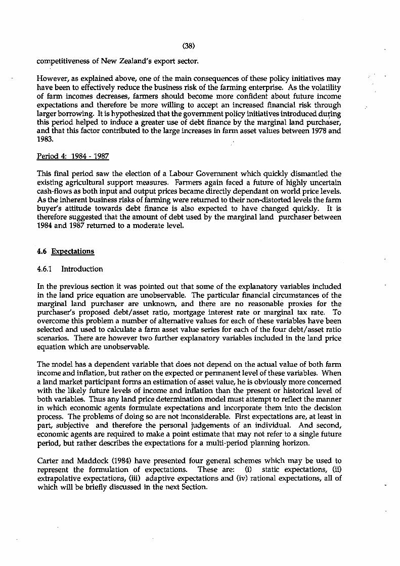
(38)

competitiveness of New Zealand's export sector.

However, as explained above, one of the main consequences of these policy initiatives mayhave been to effectively reduce the business risk of the farming enterprise. As the volatilityof farm incomes decreases, farmers should become more confident about future incomeexpectations and therefore be more willing to accept an increased financial risk throughlarger borrowing. It is hypothesized that the government policy initiatives introduced dU9ngthis period helped to induce a greater use of debt finance by the marginal land purchaser,and that this factor contributed to the large increases in farm asset values between 1978 and1983.

Period 4: 1984 - 1987

This final period saw the election of a Labour Government which quickly dismantled theexisting agricultural support measures. Farmers again faced a future of highly uncertaincash-flows as both input and output prices became directly dependant on world price levels.As the inherent business risks of farming were returned to their non-distorted levels the farmbuyer's attitude towards debt finance is also expected to have changed quickly. It istherefore suggested that the amount of debt used by the marginal land purchaser between1984 and 1987 returned to a moderate level.

4.6 Expectations

4.6.1 Introduction

In the previous section it was pointed out that some of the explanatory variables includedin the land price equation are unobservable. The particular financial circumstances of themarginal land purchaser are unknown, and there are no reasonable proxies for thepurchaser's proposed debt/asset ratio, mortgage interest rate or marginal tax rate. Toovercome this problem a number of alternative values for each of these variables have beenselected and used to calculate a farm asset value series for each of the four debt/asset ratioscenarios. There are however two further explanatory variables included in the land priceequation which are unobservable.

The model has a dependent variable that does not depend on the actual value of both farmincome and inflation, but rather on the expected or permanent level of these variables. Whena land market participant forms an estimation of asset value, he is obviously more concernedwith the likely future levels of income and inflation than the present or historical level ofboth variables. Thus any land price determination model must attempt to reflect the mannerin which economic agents formulate expectations and incorporate them into the decisionprocess. The problems of doing so are not inconsiderable. First expectations are, at least inpart, subjective and therefore the personal judgements of an individual. And second,economic agents are required to make a point estimate that may not refer to a single futureperiod, but rather describes the expectations for a multi-period planning horizon.

Carter and Maddock (l984) have presented four general schemes which may be used torepresent the formulation of expectations. These are: (i) static expectations, (ii)extrapolative expectations, (iii) adaptive expectations and (iv) rational expectations, all ofwhich will be briefly discussed in the next Section.

(39)

4.6.2 The Treatment of Expectations

(i) The static expectations behavioral equation is the most simplistic of the four generalschemes. It states that economic agents base their expectations for the value of anexplanatory variable on the actual level of that variable in the previous period. Thus,the behavioral equation is:

where: Vt" = the expected level of the variable'in period t.

This obviously assumes that the decision maker does not consider the past directionof change in the level of the variable, nor the possibility that any given observationmay be significantly different from an otherwise stable trend.

(ii) The extrapolative expectations scheme improves on the static case by including thedirection of change in the economic variable. The behavioral equation then becomes;

where Q is the coefficient of expectation.

Expectations for the future period are then equal to the current period's level plus afraction, Q, of the change between the previous two periods. H Q is positive, theexisting trend is expected to continue, while that trend is expected to be reversed ifQ is negative. The extrapolative expectations scheme becomes identical to staticexpectations if Q is equal to 0, implying that no trend information is included.

(iii) The adaptive expectations includes an error correction term as agents are assumed torevise their expectations for the future period according to the degree of error in theirprevious estimates. The expected level of the variable, V, in period t is defined as;

where 'A, is the coefficient of adaptation and (Vt-1 - V"t-l) measures the previous periods'error. The size of 'A, determines the speed with which economic agents' expectationsadjust to past errors. It may also be considered a gauge of whether or not agentsexpect the factors which contributed to the expectation error to exist in the future.

Carter and Maddock (1984) suggest that all three of these expectations hypotheseshave a common weakness in that they are not based on any underlying theory ofeconomic behaviour. Each of the schemes essentially states that the expected valueof a variable is formulated using some manipulation of past levels of that variableonly. Muth (1961), on the other hand advanced the hypothesis that economic agentswould use all of the information available to them in forming their expectations.

(iv) The rational expectation hypothesis therefore attempts to incorporate an assumedknowledge of the economic system into the formulation process. That is, the expected

(40)

value of a variable should be considered endogenous to the model, where theexpected value is equal to the equilibrium value of the explanatory variable plus theexpected value of the error term. Seed (1986) points out that although rationalexpectations has the advantage of providing a basis for calculating weights in adistributed lag, truly rational expectations require a large amount of information tobe operational.

J

Irrespective of the advantages that the rational expectations hypothesis may provide, anumber of reservations concerning the relevance of all four schemes to the land marketremain. Of most consequence is the fact that the schemes ,are essentially retrospective, andin some cases use information which may not always be available to, or considered by, theeconomic agents that the model purports to represent. Any expectations hypothesis should

. be formulated with careful regard to the economic sophistication of the relevant marketparticipants. The extrapolative, adaptive and rational expectations models may inadequatelyrepresent the way in which farm buyers form expectations, partly because they incorrectlyassume that these agents have a thorough understanding of the economic system. Thus, asHebden (1983) points out, sometimes the most naive model can (rather hUmiliatingly)perform just as well as any others.

Moreover, the relevance of these hypothetical constructs is questionable when it is knownthat the decision makers have some appreciation of what is going to happen in the nearfuture, and almost certainly use this information when forming their expectations. Forexample, at the beginning of any given year farmers usually have some knowledge of likelyproduct prices and input costs for the coming period. This information will obviously beused to help form expectations of future income, and may suggest a level of income notdiscernable from historical information alone. That the four expectations schemes describedby Carter and Maddock (1984) use past information only is a major problem.

Unfortunately, none of the research reviewed for this study has attempted to incorporate anyallowance for future predictions of the level of a variable into the formulation of expectations.It is obviously difficult to retrospectively determine what future information is known by theeconomic agents when they form expectations. Indeed, most of the reviewed studies haveempirically tested the relevance of the four general schemes, and then simply used thehypothesis which provides the best fit of the sample data. As a result, the particularexpectations scheme is often chosen with more regard to empirical accuracy rather than thetheoretical justification that each suggests.

The expectations hypotheses that are considered most relevant to this study are discussed inthe next two Sections.

4.6.3 Expectations of Returns to Total Production Assets

Selection of an expectations hypothesis that accurately reflects the way in which incomeexpectations are actually formed by land buyers is obviously an important task. From thespecified land price equation, expected income is one of the most important determinants offarm asset values and the calculated values are subsequently very sensitive to the particularexpectations scheme used. The previous section argued that the chosen hypothesis shouldbest reflect the assumed economic behaviour of the agents in the model. In this instance, themost appropriate scheme will depend on the level of economic sophistication and amountof information that farmland buyers are assumed to have. The choice should not be made

(41)

strictly on the criterion of which expectations scheme allows the best fit of the data.

The previous Section also suggested that all four retrospective hypotheses do not realisticallyrepresent the way in which farmers form expectations, since they do not permit theincorporation of all relevant future information that may be available to the agents. This isan important failing as most farmers, and certainly all marginal land purchasers are thoughtto base future income expectations on predicted future product prices and input costs. Inmany instances, these future predictions cannot possibly be implied by the returnS fromprevious periods alone. The most obvious example of this is when a government pricesupport, or input subsidy is announced. An expectatioIl& hypothesis based on historical farmreturns cannot incorporate this important information even though it is available to farmers,and almost certainly used when forming their expectations of future returns.

As a result this study will use an expectations scheme which allows for the incorporation offuture information. Actual returns to farm assets for each period, as calculated from theN.Z.M.W.B.E.S. surveys will be used as a proxy for the future periods' expected income.However, although this gives a reasonable approximation of what land market participantsmay budget on receiving in the coming year, the farmers' prediction should not be expectedto exactly equal actual returns. A constrained random error term will therefore be added tothe expected value of farm returns to allow for this anticipated prediction inaccuracy. Thereis unfortunately no research evidence available that may indicate how large the budgetingerrors have historically been, although expert opinion and experience1 suggests that an errorof 10% may be a reasonable estimate.

Previous experience also suggests that farmers incorporate a small amount of pastinformation into the formulation of expectations. That is, their estimations of the future, orpermanent level of income are based on some weighted average of last period's income andthe budgeted return for the coming period. Again there is no research evidence available tosuggest what the respective weightings may be, and the proportions used in this study mustbe arbitrarily set. Nevertheless, despite the obvious shortcomings of this scheme, it is stillthought to more realistically represent the manner in which expectations are actuallyformulated by land buyers compared to the four schemes previously discussed.

Initially, the expected level of farm income will be determined using the following behavioralequation.

YAOt = 0.3Y~_1 + (0.7Y~ + REt)

where YAOt

Y~-lY~

RE

= expected returns to farm assets in the current period, t, as formedat the beginning of that period.

= Actual returns to farm assets in the previous period.= Actual returns to farm assets in the current period t.

This value will be used as a proxy for the budgeted, or predictedreturn for the current period.

= A random error term which will be constrained to a range of ± 10%of Y~ with a mean of O.

and the period weightings will initially be set at the levels shown.

1. Dr G.A.G. Frengley, Lincoln University.

(42)

Because both the relative period weightings and the size of the random error have beenarbitrarily set, a sensitivity analysis will be carried out to establish whether the results of theanalysis are dependent on these imposed values.

4.6.4 Expectations of Inflation

The importance of choosing an expectations hypothesis which has particular regard to theassumed economic sophistication of the economic agents involved is emphasized in Section4.6.1 of this study. It is advanced that the chosen hypothesis should only use informationwhich is thought to be both available to, and considered l;>y land market participants whenformulating their expectations. Unfortunately there is ho research evidence available tosuggest which variables are actually incorporated into a land purchaser's formulation ofexpected inflation.

In a survey of expectations hypotheses used in United Kingdom models, Holden et al (1985)find that most of the expected price level models are similar to that used by the BritishTreasury. Expected inflation is calculated as a weighted average of the previous year'sinflation and the rate of growth of the money supply during the previous years. The weightsare determined by regression analysis. Thus to the extent that p;:tst money growth indicatesfuture inflation, this price expectation series may be regarded as a compromise betweenforward and backward looking expectations.

However, this hypothesis is not considered to be directly applicable to the economic agentsthat this study is attempting to model. The rate of growth in the money supply is notexpected to be used by farmland purchasers as an explanatory variable of the future inflationrate. Inclusion of this variable would necessarily require an assumption that land marketparticipants have an advanced appreciation of the macroeconomic system and its underlyingeconomic theory. It is argued that such an assumption cannot be made in this instance.

As a result, the expectations scheme to be used in this study is a second order distributed lag.This model is considered to be a more realistic representation of the way in which landowners estimate expectations of the future level of inflation. Farmers are assumed to use theobserved levels of inflation in previous time periods to form their expectation of the inflationrate in the cutrent period. The respective weights were calculated using regression analysis.

4.7 Definition of the Variables

The previously specified land price equation states that land price is some function of thereturns from the land, or more correctly, net rent. But, as has already been pointed out, timeseries data in New Zealand are not readily available. Seed (1986) suggests the alternative isto calculate proxies for land price and net rental income which will capture the effects of theunobtainable variables and maintain the relationship between the price of land and itsexplanatory variables. Although this procedure will unavoidably introduce some amount ofcomputational error into the analysis, its use is necessitated by the lack of net rental data.

The approach taken in this study is to adjust land price and net income to obtain twotheoretically comparable series. The data used for the computation of most variables is takenfrom the N.Z.M.W.B.E.S. sheep and beef farm surveys, and the period of the study was 1962- 1987. Class seven farms (representing Southland) have been chosen as the sector to bestudied. All variables are measured in nominal terms.

(43)

4.7.1 Proxy for Net Rent: Current Returns to Total Production Assets

This variable represents the return to total farm capital and is not specific to the form ofownership or the method of financing. It is calculated by adding rent, interest andmanagerial salaries to the farm cash surplus. Because this figure still contains a return tolabour and management, an assessed management reward has been deducted to obtain anestimate of residual return attributable to production assets alone. The N.Z.M.W.B.E.S.calculates management reward by adding one percent of total farm capital to the currentaverage wage for a married couple.

4.7.2 Proxy for Land Value: The Value of Total Production Assets

Because the chosen proxy for net rent is an aggregate return to total farm capital, it cannotbe justifiably compared to land value alone. Thus, the value of total production assets iscalculated by adding the value of livestock, plant and machinery, and working capital to theproperty's capital value, less the value of the dwelling. The use of this proxy series avoidsthe need to calculate a separate return to all of the other assets so as to extract a return thatis solely attributable to land. An accurate return to assets such as livestock, plant andmachinery would require significantly more data in order to be accurately quantified.

4.7.3 Proxy for the Inflation Rate: Consumer Price Index

In this study the percentage change in the Consumer Price Index has been chosen as ameasure of the overall inflation rate in the general economy. This index provides the bestindication of how the real value of outstanding debt is reduced by inflation.

4.7.4 Proxyfor the Rate of Income Tax: The Highest Marginal Tax Rate

The effective income tax rate faced by the marginal land purchaser is unobservable.However, it is anticipated that the highest marginal tax rate is most applicable as it reflectsthe high income earning position that the marginal land purchaser is assumed to hold.

4.7.5 Proxy for the Opportunity Cost of Equity: Long Term Government Security Yields

The chosen proxy for this variable is thought to have a similar risk and temporal profile asequity investment in farmland. The chosen series has also been used as it is one of only afew truly consistent long term series.

4.7.6 Proxy for the Cost of Debt: Rural Bank Mortgage Interest Rate

This proxy series reflects the concessional interest rates available to farmland investorsthrough most of the period covered by the analysis.

4.7.7. Potential Problems with the Data

In his study of land price determination, Seed (1986) also used N.Z.M.W.B.E.S. data andpointed out that some potential biases may arise due to the way in which it is recorded. Hesuggests that farm incomes may be biased downwards because capital expenditure cannotbe easily disaggregated from general expenditure. As a result, such expenditures may beincluded in repairs and maintenance and thereby reduce the observed, or calculated level of

(44)

farm income.

Seed further suggested that in periods of high product prices, and subsequently high grossincomes farmers may increase expenditure on several capital items in an effort to reducetaxable income. Or conversely, in years of low gross incomes farmers may limit maintenanceexpenditures such as fertiliser applications in an attempt to preserve an adequate incomelevel. In both of these cases expectations of income may differ significantly from the actualrecorded income levels. )

Although both of these factors are likely to introduce sOp\e inaccuracies into the analysis,there is a more important concern regarding the use of the N.Z.M.W.B.E.S. surveys as thedata source. The land price equation has been specified with respect to the marginalfarmland purchaser. The relevant explanatory variables are however taken from a surveysample and, in effect represent average levels of those variables. As such, the proxy seriesfor net rent is expected to consistently under-estimate the level of income obtained bymarginal land purchasers, who are expected to perform better than average. TheN.Z.M.W.B.E.S data is however the only consistent data series available.

CHAPTER 5

RESULTS OF THE ANALYSIS

5.1 Introduction

The hypothesized determinants of farm asset values for the N.Z.M.W.B.E.S. class sevensample farms are incorporated into a land price equation in section 4.4, and includes the levelof debt used by the marginal land purchaser as an explanatory variable. Unfortunately, theimportance of financial leverage in the farm value determination process cannot be directlyestimated. As explained in section 4.5.1, the relevant ,circumstances of the marginal landpurchaser are not directly observable and nor do they have identifiable proxies. Mostimportantly there is no information available concerning the marginal land purchaser'sproposed debt/asset ratio. This factor precludes econometric estimation of their impact onland price.

As a result, an alternative analytical method is proposed in section 4.5.2 which involves thecalculation of four land value series that differ only in respect to the assumed debt/assetratios used in the calculations. With all other variables held constant these calculated landvalue series can be statistically compared to the proxy series of actual land values.Consequently some assessment can be made of the impact that financial leverage has had onfarm asset values during the 1962 - 1987 period.

Because direct estimation is not possible, some alternative descriptive statistics are neededto measure the relative ability of each of the calculated value series to accurately reproducethe proxy series of actual values. Two main accuracy measures are used in this study. Theyare the correlation coefficient and Theil's inequality coefficient, both of which are describedin section 5.2. These are then applied to the class seven data in section 5.3 to determinewhich of the four debt!asset ratio alternatives provides the best fit to the actual asset valuedata. In section 5.4 the same descriptive statistics are used to estimate how the hypothesizedimpactof financial leverage may have changed during the 1962 -1987 period, by individuallyanalyzing the four sub-periods identified in section 4.5.3.

5.2 Statistical Measures of Accuracy

5.2.1 Correlation Coefficient

The correlation coefficient is normally used as a measure of the linear relationship betweentwo variables. The coefficient of correlation, r, is a relative measure of the linear associationbetween these two variables. It may vary from 0, which indicates no correlation to ± I,which indicates perfect correlation. When the correlation coefficient is greater than 0, theyare said to be positively correlated. However, it is important to note that an apparentrelationship between the two variables does not necessarily infer that changes in the valueof one of the variables depends upon, or is caused by changes in the value of the othervariable.

Makridakis et al. (1982) suggest that the correlation coefficient can be correctly interpretedin two ways. First, the sign of r shows the direction of the relationship between thevariables. And second, the strength of the association is measured by the absolute value of

(45)

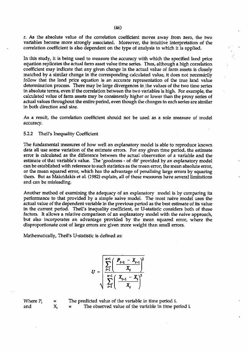
(46)

r. As the absolute value of the correlation coefficient moves away from zero, the twovariables become more strongly associated.. Moreover, the intuitive interpretation of thecorrelation coefficient is also dependent on the type of analysis to which it is applied..

In this study, it is being used. to measure the accuracy with which the specified. land priceequation replicates the actual farm asset value time series. Thus, although a high correlationcoefficient may indicate that any given change in the actual value of farm assets is closelymatched. by a similar change in the corresponding calculated. value, it does not necessarilyfollow that the land price equation is an accurate representation of the true land valuedetermination process. There may be large divergences in,the values of the two time seriesin absolute terms, even if the correlation between the two variables is high. For example, thecalculated. value of farm assets may be consistently higher or lower than the proxy series ofactual values throughout the entire period, even though the changes in each series are similarin both direction and size.

As a result, the correlation coefficient should not be used as a sole measure of modelaccuracy.

5.2.2 Theil's Inequality Coefficient

The fundamental measures of how well an explanatory model is able to reproduce knowndata all use some variation of the estimate errors. For any given time period, the estimateerror is calculated. as the difference between the actual observation of a variable and theestimate of that variable's value. The 'goodness - of -fit' provided by an explanatory modelcan be established. with reference to such statistics as the mean error, the mean absolute error,or the mean squared. error, which has the advantage of penalising large errors by squaringthem. But as Makridakis et al. (1982) explain, all of these measures have several limitationsand can be misleading.

Another method of examining the adequacy of an explanatory model is by comparing itsperformance to that provided. by a simple naive model. The most naive model uses theactual value of the dependent variable in the previous period as the best estimate of its valuein the current period. Theil's inequality coefficient, or U-statistic considers both of thesefactors. It allows a relative comparison of an explanatory model with the naive approach,but also incorporates an advantage provided. by the mean squared error, where thedisproportionate cost of large errors are given more weight than small errors.

Mathematically, Theil's U-statistic is defined. as:

U=

Where Piand

= The predicted value of the variable in time period i.= The observed value of the variable in time period i.

(47)

The numerator can be defined as the relative prediction error while the denominatordescribes the relative changes in the observed variable.

For a perfect predictor the calculated and observed values of the variable are equal in eachtime period, thereby forcing the value of the numerator term equal to zero. In this case thevalue of Theil's V-statistic will also equal O. Alternatively the V-statistic will have a valueof 1 only if the errors in the calculated values are the same as those that would be optainedby using the observed value in the previous period as the estimate of that variable's valuefor the current period.

The ranges of the V-statistic are summarised by Makridakis et al. as follows. If,V =1, then the estimation model being evaluated is no better than a naive model.

V < 1, then the estimation model being used is better than a naive method. Thesmaller the V-statistic the better the estimation model is relative to the naive method.

V> 1, there is no point in using the specified estimation model, as the naive methodwill product better results.

Another method of evaluating the adequacy of an estimation model also provides anexplanation of the reasons why the calculated V-statistic differs from zero. This involves aregression of the actual changes in the observed variable on the changes in the estimatedvalues. If th~ specified model produces estimates which exactly replicate the observed valuesof a variable, then the regression intercept will equal 0 and the slope coefficient will equal1. The calculated V - statistic will also equal zero. However when the model producesresults which are less than perfect, Theil (1966) suggests the calculated mean square error canbe broken down into three parts.

The first, called the bias proportion corresponds to that part of the mean square errorresulting from a tendency to produce estimates which are either too high or too low, and isreflected by the extent to which the regression intercept differs from zero. The secondproportion of the mean square error is measured as that due to systematic influences. It ismeasured by the extent to which the slope coefficient in the regression equation differs from1. The third, called the disturbance proportion reflects that part of the mean squared errorresulting from an unpredictable error, which in turn is measured by the variance of theresiduals from the regression equation. The specified explanatory model is considered to bemore accurate if the difference between the V - statistic and zero is the result of errorexplained by this third category. The proportion of error due to the other two parts willtherefore then be approaching zero.

Theil (1966) also gives an alternative composition of the mean squared error, where it isbroken down into bias, variance and covariance proportions. However, because thisalternative has been shown by Granger and Newbold (1973) to have questionable meaning,the first decomposition explained above will be used in this study.

5.3 The Impact of Financial Leverage on Farm Asset Values, 1962 - 1987

Vsing the land price equation presented in Section 4.4 of this study, the four alternative series

(48)

of farm asset values were calculated and subsequently compared to the proxy series of actualvalues. The primary objective of the analysis is to establish which of the four assumeddebt/asset ratios provides a series of calculated values that most accurately represents theobserved time series data. The Time Series Processor (T.S.P.) econometric package was usedto perform the analysis.

Before the statistical results are reported and discussed, it is important to reconsider spmeproblems and limitations the chosen analytical method presents. The specified land priceequation is a non-parametric deterministic model. As no allowance is made for uncertainty,the model used in this study is open to similar criticisms ~s those Seed (1986) levelled at themodel used by Leathers and Gough (1984). There is no relationship estimated between theexplanatory variables and the dependent variable, and as a result the relative impact of eachvariable on the calculated value of total farm assets is the direct result of its mathematicalspecification.

However as previously discussed, direct econometric estimation of the relationship betweenthe explanatory and dependent variables is not possible because several of the includedexplanatory variables are unobservable. The analytical approach taken in this study is adirect consequence of this problem. Thus, any conclusions made concerning the apparentimpact of financial leverage on farm asset values are reliant on an assumption that thespecified land price equation is a close representation of the true but unknown valuedetermination process. This is obviously a crucial assumption and one that must depreciatethe potency of any conclusions drawn from the analysis.

With regard to this factor, a summary of the statistical results is reported in table 5-1. Thecalculated farm asset value series which provides the most accurate comparison to the proxyseries of actual values over the entire period uses the assumed debt/asset ratio described bycase 3. Of the four alternative calculated scenarios, case 4 provides the highest correlationcoefficient of 0.8925, which suggests that this series is the most strongly associated with theactual value series. However, the calculated U-statistic for case 4 is the highest of all thealternatives at 0.8684, indicating that this estimation model is least able to replicate theobserved series of farm asset values. Decomposition of the calculated error shows thatalthough the relative changes in the actual values of farm assets are closely matched by thechanges in the case 4 calculated values, the calculated values are consistently and appreciablylarger than the proxy series. The tendency of this model to overestimate farm asset valuesis reflected by the high calculated proportion of the error caused by bias. It is thereforesuggested that the amount of debt used by land purchasers during the 1962 - 1987 periodwas significantly lower than the 100 percent level assumed in the case 4 calculated series.

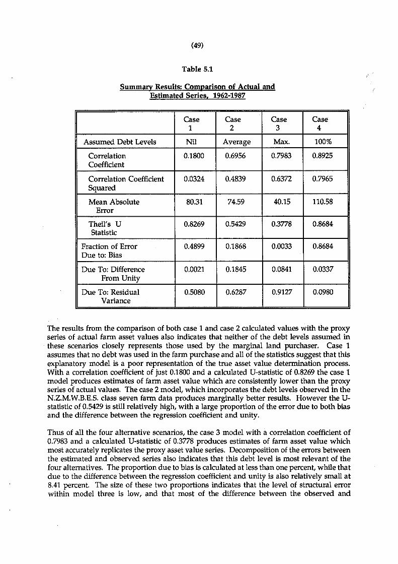
(49)

Table 5.1

Summary Results: Comparison of Actual andEstimated Series, 1962-1987

Case Case Case Case1 2 3 4

Assumed Debt Levels Nil Average Max. 100%

Correlation 0.1800 0.6956 0.7983 0.8925Coefficient

Correlation Coefficient 0.0324 0.4839 0.6372 0.7965Squared

Mean Absolute 80.31 74.59 40.15 110.58Error

Theil's V 0.8269 0.5429 0.3778 0.8684Statistic

Fraction of Error 0.4899 0.1868 0.0033 0.8684Due to: Bias

Due To: Difference 0.0021 0.1845 0.0841 0.0337From Vnity

Due To: Residual 0.5080 0.6287 0.9127 0.0980Variance

The results from the comparison of both case 1 and case 2 calculated values with the proxyseries of actual farm asset values also indicates that neither of the debt levels assumed inthese scenarios closely represents those used by the marginal land purchaser. Case 1assumes that no debt was used in the farm purchase and all of the statistics suggest that thisexplanatory model is a poor representation of the true asset value determination process.With a correlation coefficient of just 0.1800 and a calculated V-statistic of 0.8269 the case 1model produces estimates of farm asset value which are consistently lower than the proxyseries of actual values. The case 2 model, which incorporates the debt levels observed in theN.Z.M.W.B.E.S. class seven farm data produces marginally better results. However the Vstatistic of 0.5429 is still relatively high, with a large proportion of the error due to both biasand the difference between the regression coefficient and unity.

Thus of all the four alternative scenarios, the case 3 model with a correlation coefficient of0.7983 and a calculated V-statistic of 0.3778 produces estimates of farm asset value whichmost accurately replicates the proxy asset value series. Decomposition of the errors betweenthe estimated and observed series also indicates that this debt level is most relevant of thefour alternatives. The proportion due to bias is calculated at less than one percent, while thatdue to the difference between the regression coefficient and unity is also relatively small at8.41 percent. The size of these two proportions indicates that the level of structural errorwithin model three is low, and that most of the difference between the observed and

(SO)

calculated values is a result of residual variance or unpredictable error.

As explained in Section 4.5.2, the debt/asset ratios described by case 3 are based on themaximum level of debt that the New Zealand Rural Banking and Finance Corporation willallow a mortgagee to borrow, measured as a percentage of total farm asset value. Duringthe 1962 and 1987 period that limit has ranged between 31.3 percent and 49.7 percent. Theresults of this analysis therefore provides evidence to suggest that the use of fina,ncialleverage has been an important factor in the determination of farm asset values. Theadvantages of using debt finance in a farm purchase have been examined in Section 4.4 ofthis study. It was argued that the effects of both tax deductibility of interest payments anddebt erosion reduce the investor's effective required rate" of return, and that the capitalizedvalue of farmland for a farmer who uses debt is subsequently higher than that calculated foran all equity investment. That the case 3 model has been shown to produce the mostaccurate estimates of farm asset values supports the hypothesis advanced in Section 4.5.3,which argues that the marginal land purchaser was expected to use a relatively high levelof debt finance to take advantage of its potential benefits. "

However, it was also hypothesized in Section 4.5.2 that the impact of financial leverage hasnot remained constant over the analyzed twenty five year period. Comparison of the fouralternative calculated value series with the observed series shows that none of the assumeddebt levels appears to consistently represent that used by the marginal land purchaserfor theentire twenty five years period. In fact, the case 3 model consistently overestimates the valueof farm assets for the first nineteen years of the 1962 - 1987 period, indicating that the levelof-debt used by the marginal land purchaser up until 1981 was less than that represented bycase 3. A number of possible factors which have governed the level of debt used in an assetpurchase have been suggested. The one of most consequence is thought to have beengovernment agricultural policy which has changed significantly throughout the analyzedperiod. But before this question is addressed, the sensitivity of the reported results to theway in which income expectations are expressed in this study are-examined.

The assumed expectations formulation process attempts to incorporate information aboutfuture returns which is known by the land purchaser at the beginning of each period, butwhich is not expressed in historical net returns data. Thus actual returns to farm assets foreach period have been used as a proxy for the budgeted returns in that period, and aproportion of this figure is added to a proportion of net income from the previous period togive an estimate of the income level to be capitalized. This expectations scheme is expressedin Section 4.6.3 as,

YAOt = 0.3 YAt-1 + (0.7 Y~ + RE)

where YA\ = The expected level of net income for time period t.Y~ = the actual level of net income in the time period t, which acts as a

proxy for the budgeted level of income in period t.and, RE = a random error term which has a range of ± 10% of YA, and a

mean of zero.

Both the range and mean of the error term have been set with reference to expert opiniononly. It is suggested that the difference between farmers' budgeted estimates of net incomefor the coming period and the actual realized levels of income has a range of ± 10 percent,and that for any given sample of farmers the budget errors would have a zero mean. The

(51)

calculated series of income expectations used in the analysis presented earlier has thereforealso used an error term with a value of zero.

The sensitivity analysis examines whether or not the statistical results, and subsequentconclusions drawn from the previous analysis are dependent on this assumption. The fouralternative farm asset value series were recalculated allowing for a budget error of plus andminus ten percent of YAv and then compared to the observed series using the, sametechnique as previously described. Both sets of results are reported in Appendix 4, and theseshow that the changes to the expected level of income do not alter the conclusions reachedearlier. In both cases the third alternative debt level pr<?duces estimates of farm asset valuewhich most accurately reflect the proxy series of actual values. In fact the relative accuracyof each of the four alternative cases is not affected by the changes to the error term.

5.4 The Hypothesized Changes in Debt Levels Between 1962 and 1987

The analyzed period of 1962 - 1987 has been split into four distinct sub-periods to examinethe hypothesis advanced in Section 4.5.3. This suggests that there are many possible factorswhich may affect the fraction of debt used by the marginal land purchaser, other than theadvantages of tax deductibility and debt erosion. The level of government support measuresis expected to be the most influential of these factors. As explained in Section 4.5.3,government policy initiatives which are designed to either boost or maintain net incomesmay have an effect other than merely increasing the current profitability of farming. Thesepolicies have also had an impact on the level of debt used in a farm purchase because of theway in which they affected the variability, and consequently the risk of cash-flows fromfarming. It is suggested that as more income support schemes are implemented the level ofbusiness risk faced by a farmer is reduced, and a higher level of debt finance is subsequentlyemployed in land purchases.

Thus, the changes in government agricultural policy during the 1962 - 1987 period, asobserved by Le Heron (1987) were used to identify a number of sub-periods in which thelevel of debt used by the marginal land purchaser may have changed. The four chosenperiods are described in Section 4.5. together with the corresponding level of debt thoughtto be most relevant in each particular period. The same analytical procedure as that appliedto the data for the entire twenty five year period was used to examine this hypothesis, andthe sumIilary results are presented and discussed below.

5.4.1 Period 1: 1962 - 1968

During this period, farmers experienced relatively volatile farm incomes, a consistently lowrate of inflation, and received relatively little government income assistance. As a result, itis suggested in Section 4.5.3 that the level of financial leverage employed by farm purchaserswas also low. Examination of the summary analytical results presented in table 5.2 tends tosupport this argument.

The calculated U-statistics for both the case 3 and case 4 models are relatively high, at 0.7111and 2.5833 respectively. That the majority of the error between the estimated and observedvalues is caused by bias indicates that the levels of debt that these two cases represent aresignificantly higher than that used by the marginal land purchaser during the 1962 - 1968period.

(52)

Table 5.2


Case Case Case Case1 2 3 4 )


Correlation - 0.1061 -0.1547 0.1019 -0.0462Coefficient



Theil's U 0.4575 0.4039 0.7111 2.5833Statistic


Due To: Difference 0.0850 0.3592 0.1586 0.0673From Unity


However, although the statistical results from the first two models are quite similar, modeltwo provides the more accurate representation of the proxy series of actual farm asset values.Case 1 produces a U-statistic of 0.4575 while that for the case 2 model is marginally lowerat 0.4039. The highest proportion of the errors between the calculated and observed seriesis due to bias in both cases. Examination of the two calculated series of farm asset valuesshows that the case 1 model consistently underestimates the proxy series of actual valueswhile the case 2 values consistently overestimates these values. The degree of financialleverage actually used by the marginal land purchaser between 1962 and 1968 is thereforeexpected to have fallen between the levels of debt assumed by cases 1 and 2.

5.4.2 Period 2: 1969 - 1977

The changes in both net farm incomes and government agricultural policy during the periodare described in Section 4.5.3 It was argued that the combined effect of these two factors,together with a significantly higher level of inflation which persisted after the 1973 oil-shockacted to encourage a greater use of financial leverage in this period than that used between1962 and 1968.

,/

(53)

The summary results from the period 2 analysis are reported in table 5.3, and indicate thatthe case 2 model again provides the most accurate calculations of total farm asset value. Theassumed debt level represented by this scenario is the average debt/asset ratio observed inthe N.Z.M.W.B.E.S. class seven data. However, even though the case 2 model has beenfound to most accurately replicate the proxy series of actual asset values in both the 1962 to1968, and 1969 to 1977 periods, the results still indicate that some increase in the level of debtused by land purchasers has occurred during the latter period.

Table 5.3




Correlation 0.2478 0.4879 0.6723 0.6361Coefficient







Case 1 has a calculated V-statistic of 0.5364 while that for the case 2 model is measured at0.3542. The difference between these two statistics is higher than that observed between theV-statistics for cases 1 and 2 in the previous period. The relative accuracy of the case 2model is also improved when it is applied to the 1969 - 1977 period. These factors providesome evidence to suggest that the relevant level of debt used by the marginal land purchaserhas increased during this second sub-period. First, the tendency of the case 1 model tounderestimate farm asset value is greater in this time period than that observed between 1962and 1968. This suggests that the level of debt represented by case 1 is even moreinappropriate for the 1969 -1977 period than it was previously. Conversely, the case 2 modelproduces more accurate results than those obtained in the analysis of period 1 when it is

(54)

applied to the second sub-period. Thus although it continues to overestimate the observedvalues of farm assets, the degree of overestimation is reduced when using data from between1969 and 1977.

5.4.3 Period 3: 1978 - 1983

As described earlier in Section 4.5.3 of this study, the scale of government support measuresfor agriculture reached its peak during the 1978 - 1983 period. As well as the introductionof the Supplementary Minimum Price Scheme, this period also saw the initiation of two othermajor policies which were designed to actively encqurage farm development andintensification. The government was effectively guaranteeing future net farm income at an,adequate' level, and thereby encouraging farmers to increase investment in both theirexisting properties and in additional land acquisition.

It is argued that these measures may have also encouraged a greater utilization of debt fundsby the marginal land purchaser. This factor is hypothesized to have subsequentlycontributed to the large increases in total farm asset values over the 1978 -1983 period. Thesummary statistical results of the period 3 analysis, which are presented in table 5.4, aretherefore expected to reveal that the level of debt most relevant in this period is greater thanthat observed in the previous two periods.

Of the four alternative capital structure scenarios, the case 3 model provides the mostaccurate comparison of calculated and observed farm asset values for the 1978 -1983 period.However, the calculated V-statistic for this model is relatively high at 0.4259, and thecalculated values are neither consistently higher or lower than the associated series of actualvalues. This may indicate that the levels of borrowed funds used by the marginal landpurchaser did not remain stable between 1978 and 1983. Rather, it is suggested they mayhave increased rapidly, from below the debt levels represented by case 3 in 1978 to abovethat level by the end of the six year period.

Thus, although both the government income support measures and developmentencouragement schemes were announced at the beginning of this sub-period in 1978, theseresults may indicate that the policies did not immediately influence the level of debt used infarmland purchases.

5.4.4 Period 4: 1984 - 1987

The summary analytical results for the last sub-period are reported in table 5.5, and areexpected to reveal that the levels of debt used by a marginal land purchaser decreasedsignificantly in this period compared to the previous 1978 - 1983 period. Section 4.5.3describes that after the election of a Labour Government in 1984, the majority of existingagricultural support measures were quickly dismantled. Both product price and farm incomeguarantees were discontinued, forcing farmers to again face a future of highly uncertain cashflows. As the inherent business risks of farming were returned to their non-distorted levels,tne farm buyer's attitude toward debt finance is expected to have changed quickly.

However, the analytical results suggest that the decrease in debt levels during this period isnot as great as that hypothesized. The case 3 model again provides the most accurateestimates of total farm asset value with a calcuIa:ted V-statistic of 0.2034.

(55)

Table 5.4


Case Case Case Case'1 2 3 4


Correlation 0.5740 0.0909 -0.3938 0.5869Coefficient







(56)

Table 5.5



Assumed Debt Levels Nil Average' Max. 100%

Correlation -0.4579 -0.5638 0.8588 0.8536Coefficient







The debt/asset ratios represented by case 3 are relatively high, measured as the maximumamount of debt finance that the R.B.F.e. will allow a mortgagee to borrow. Moreover, theresults indicate that the case 3 model consistently underestimates the observed values of famlassets for all four years. As such, the level of debt actually used by the marginal landpurchaser may have been greater than that assumed in the case 3 model. The evidencetherefore suggests that the use of financial leverage has not changed significantly betweenthe 1978 - 1983 and 1984 - 1987 periods.

CHAPTER 6

IMPLICATIONS FOR AGRICULTURAL POLICY

In his study of land price determination in New Zealand, Seed (1986) found that realfarmland prices were positively related to expected net rental income. That is, an increasein farmers' expectations for future income, irrespective of how that increase is generated, willlead to an increase in the real price of farmland. These findings led Seed to suggest that anincrease in expectations of real farm incomes caused by some form of central governmentagricultural assistance would therefore contribute to an increase in the real price of land.Thus, the introduction of product price supports, inl;:ome smoothing schemes or inputsubsidies which may be designed to assist a particula'r group such as entry level farmers,may only serve to improve the wealth position of existing land owners. As a result, theability of entry level farmers to actually enter the industry may be reduced during periodsof rapidly rising farmland prices as they may not have the required finance or the necessarycash flow to support a farm purchase.

The policy implications of this study are similar to those advanced by Seed. The analyticalresults have provided some evidence to suggest that the level of debt funds used by themarginal land purchaser is an important determinant of farm asset value. By incorporatingborrowed finance into the capital structure, the required rate of return of the marginal landpurchaser is reduced due both to the tax deductibility of interest payments and the inflationinduced effect of debt erosion. As with any investment, if the required rate of return isreduced then the price an intending asset owner can afford to pay must increase. Thesefindings have important implications for policies which are designed to ameliorate thepossible cash flow problems of prospective new farm buyers.

Leathers and Gough (1984) suggest that liquidity is the most important concern of farmersduring periods of high inflation because current income is typically too low to service amortgage on farm assets. Existing farmers who have either low debt loads or a significantsource of non-farm income are therefore in the best position to purchase additional farmland.Individuals who entered farming for the first time during these periods usually did sothrough inheritance. In an attempt to improve the ability of potential new farmers topurchase land, the New Zealand Government offered concessionary finance to farm buyersthroughout the 1962 -1987 period. Interest rates on Rural Bank loans for farm purchase wereup to fifty percent lower than commercial rates, thereby reducing the debt servicingrequirements for entry level farmers. Importantly however, the concessionary finance wasnot restricted to first farm buyers, as existing farmers could also obtain finance with similarterms to purchase additional land.

It is therefore suggested that the government's lending policy which was promulgated toreduce the liquidity problems of prospective new farmers and subsequently improve theirability to purchase a farm actually made it more difficult to enter the industry. Individualswith low current debt loads or significant off-farm incomes had access to a source of debtfinance which effectively amplified the taxation advantages of using financial leverage in afarm purchase. With the cheap Rural Bank. loans, existing farmers may have beenencouraged to use higher levels of debt to acquire additional land and, as the reqUired rateof return on the new investment was reduced, the amount an existing farmer could affordto pay was increased. Thus, the concessionary finance may have helped to create a level offarm values which were beyond the reach of new entry farmers.

(57)

(58)

The second policy implication of this study is closely related to the first. The level ofgovernment assistance to agriculture, as described by Le Heron (1979) reached a peak duringthe late 1970's and early 1980's. That period saw the introduction of such policies as theSupplementary Minimum Price Scheme, the Livestock Incentive Scheme and the LandDevelopment Encouragement Loan Scheme which were designed to maintain current farmincomes and to encourage increased investment in agricultural production. Seed (1986)concluded that the effect of these policies was to increase the expected level of future netincome and subsequently contribute to an increase in farm asset values. However,' thatauthor also concluded that the observed increases in land prices between 1977 and 1982 didnot appear to be totally attributable to the raised income ~xpectations of farmers.

The results of this study indicate that the level of debt used by the marginal land purchaserincreased during this period, and it is suggested that this factor may explain a significantamount of the observed increases in farmland prices. It may be argued that theGovernment's policy initiatives at the time contributed to the increased use of debt financedue to the way in which they affected the perceived risk of farming. As the product pricesupports effectively reduced the variability of farm incomes, the amount of business riskfaced by a farmer also decreased. The income guarantees may have therefore encouragedthe marginal land purchaser to incorporate a higher level of debt finance into his capitalstructure, and following the theoretical impact of financial leverage, added to an increase infarm asset values.

Thus, government policies which are intended to support or improve current farm incomesmay only act to compound the problem. First, farmland values may be increased as farmers'expectations of future income are raised, and second, the policies may encourage greater useof financial leverage which has also been shown to produce an increase in farm asset values.This only serves to exacerbate the original problem of low current farm returns and arelatively high return in the form of capital gains.

REFERENCES

Abbreviations Used in This Bibliography

AAEAAAESAJAEAERJFEWJAE

American Agricultural Economics Association.Australian Agricultural Economics Society.American Journal of Agricultural Economics.American Economic Review.Journal of Farm Economics.Western Journal of Agricultural Econom'cs.

Alston, J.M. (1985), "An Analysis of the Growth of U.S. Farmland Prices, 1962-82".Contributed paper presented at AAES Conference, Armidale, February 12-14.

Bergland, Olvar and Alan Randall (1984), "Land Prices, Capital Gains and the Returns toFarmland Ownership". Selected paper at the summer meetings of the AAEA, CornellUniversity, August 5-8.

Burt Oscar (1986), "Econometric Modeling of the Capitalization Formula for FarmlandPrices". AJAE 68, pp 10-26.

Bhatia, K.B. (1972), "Capital Gains and the Aggregate Consumption Function". AER 62, pp866-879.

Carter, M and D. R Maddock (1984), Rational Expectations: Macroeconomics for the 1980's.Macmillan Houndmi1ls.

Castle, E.N. and I. Hoch (1982), "Farm Real Estate Price Components,1929-1978". AJAE 64,pp 8-18.

Chryst, W.E. (1965), "Land Values and Agricultural Income: A Paradox?" JFE 47, pp 1265-. 1273.

Doll, J.P. and R Widdows (1981), "Capital Gains Versus Current Income in the FarmingSector: Comment". AJAE 63, pp 730-733.

-------------- (1982b), "The Value of Agricultural Land in the U.S: Some Thoughts andConclusions". ERS staff report No. AGES 830124, Washington DC.

----------- (1982c), "Four Econometric Models of the U.S. Farmland Market: AnUpdating With Comparisons". ERS staff report No. AGES 820702, Washington DC.

Dunford, RW. (1980), "The Value ofUnrealised Farmland Capital Gains: Comment". AJAE63, pp 260-262.

Feldstein, M. (1980a), "Inflation, Tax Ru1es and the Stock Market". JME 6, pp 309-331.

(59)

(60)

.---------- (1980b), "Inflation, Portfolio Choice and the Prices of Land and Corporate Stock".AJAE 62, pp 910-916.

Granger, C.W.J. and P. Newbold (1973), "Some Comments on the Evaluation of EconomicForecasts". Applied Economics, Vol. 5, pp. 35-47.

Harris, D.G. (1979), "Land Prices, Inflation and Farm Income: Discussion". AJAE 61, pp '1051106.

Hebden, J. (1983), Applications of Econometrics. Philip Allan, Oxford.

Holden, 1<:.; D.A. Peel and J.L. Thompson (1985), Expectations: Theory and Evidence.MacMillan Publishers.

Johnston, J. (1984), Econometric Methods. Third Edition. McGraw Hill, Tokyo.

Just, RE. (1988), "The Explanation of Farmland Prices". Prepared for Agricultural EconomicsSeminar, August 1988, Davis University, California.

Kotler, P. (1986), Principles of Marketing. Third Edition, Prentice Hall, New York.

Leathers, K.L. and J.D. Gough. (1984), "Farmland Pricing in an Inflationary Economy withImplications for Public Policy". AERU Research Report No.162, Lincoln College.

Lee, W.P. (1976), "A Capital Budgeting Decision Model for Evaluating Farm Real EstatePurchases". Canadian Farm Economics 11, pp 1-10.

Lee, W.F. and N. Rask. (1976), "Inflation and Crop Profitability: How Much Can Farmers PayFor Land?" AJAE 58, pp 786-989.

Le Heron, R (1989), "A Political Economy Perspective on the Expansion of New ZealandLivestock Farming, 1960-84: Part 1, Agricultural Policy". Journal of Rural Studies, Vol.5, No.1, pp 33-43.

Makridakis, S.; S.c. Wheelwright and V.E. McGee. (1982), Forecasting, Methods andApplications. 2nd Ed. John Wiley and Sons.

Martin, W.J. and E.O. Heady (1982), "Inflationary Expectations and the Value of U.S. FarmReal Estate: Some Consistent Estimates". Contributed paper to the SouthernAgricultural Economics Association Meetings, February 1982, Orlando, Florida.

Melichar, E. (1979), "Capital Gains Versus Current Income in the Farming Sector". AJAE 61,pp 1085-1092.

----------- (1983), "Farm Wealth Origins, Impact and Implications". W.I. Myers MemorialLecture. Department of Agricultural Economics, Cornell University, Ithaca.

Muldoon, Hon. RD. (1982), Financial Statement. Presented 5 August 1982, House ofRepresentatives, Government Printer, Wellington.

(61)

Muth, J.F. (1961), "Optimal Properties of Exponentially Weighted Forecasts". Journal of theAmerican Statistical Association 55, pp 299-306.

Newman, D.L. (1986), "The Formulation of a Procedure to Facilitate the Analysis of FarmAccounting Statements". Unpublished Thesis, College of Business, California StateUniversity, Chico.

New Zealand Meat and Wool Board Economic Service. Sheep and Beef Farm Survey, 1960/61- 1986/87.

Plaxico, J.S. (1979), "Implications of Divergence in Sources of Returns in Agriculture". AJAE61,pp 1098-1102.

Plaxico, J.S. and D.D. Kletke (1979), "The Value of Unrealised Land Capital Gains". AJAE 66,pp750-754.

Pope, C.A. III (1985), "Agricultural Productive and Consumptive Use Components of RuralLand Values in Texas". AJAE 67, pp 81-86.

Pope, c.A. III and H.C. Goodwin (1984), "Impacts of Consumptive Demand on Rural LandValues". AJAE 66, pp 750-754.

Pope, RD.; RA. Kramer; RD. Green; B.D. Gardner (1979), "An Evaluation of EconometricModels of U.S. Farmland Prices". WJAE 4, pp 107-119.

Reinsel, RD. and E.!. Reinsel. (1979), "The Economics of Asset Values and Current Incomein Farming". AJAE 61, pp 1093-1097.

Robison, L.J.; D.A. Lins and R Venkataraman (1985), "Cash Rents and Land Values in U.S.Agriculture". AJAE 67, pp 794-805.

Schofield, W.H. (1961), "The Land Price Paradox". Contributed paper presented at theAmerican Agricultural Economics Association meeting, August 1961, Ft Collins,Colorado.

Seed, P.G. (1986), "A Study of the Determinants of Fattening and Grazing Farm Land Pricesin New Zealand, 1962-1983". Unpublished Masterate Thesis, Department ofAgricultural Economics, Lincoln College.

Shalit, H. and A. Schmitz (1982), "Farm Accumulation and Prices". AJAE 64, pp 710-719.

Statistics Department, Abstract of Statistics, (Various), Government Printer, Wellington.

Stevens, N.Z. (1978), "Rising Farmland Prices and Falling Farm Earnings: Is Agriculture inTrouble". Economic Review. Federal Research Bulletin of St Louis, Vol. 60, No.5.

Theil, H. (1966), Applied Economic Forecasting. North-Holland

Valuation Department, "Rural Real Estate Market in New Zealand". (Various), ResearchPaper, Valuation Department, Wellington.

RESEARCH REPORT

180 labour Mobility Between New Zealand and Australia, R LSt Hill. 1986

181 Survey of New Zealand Farmer Intentions and Opinions,November 1985-January 1986, JG Pryde. PJ McCartin.1986

182 A Financial and Economic Survey of South Auckland TownMilk Producers and Factory Supply Dairy Farmers, 198485, A.G. Moffitt. 1986

183 An Economic Survey of New Zealand Town MilkProducers, 1984-85, A. G Moffitt. 1986

184 An Economic Survey of NZ Wheatgrowers: FinancialAnalysis, 1984-85; A.D. Lough. PJ McCartin. 1986

185 The Effect on Horticulture of Dust and Ash: ProposedWaikato Coal-Fired Power Station, PA. McCrea. October1986

186 A 'Study of the Determinants of Fallening and GrazingFarm Land Prices in New Zealand, 1962 to 1983. PGSeed. RA Sandrey. B.D. Ward. December 1986

187 Farmers' Responses to Economic Restructuring inHurunui and Clutha Counties: Preliminary Analysis ofSurvey Data. JA. Fairweather. July 1987

188 Survey of NZ Farmer Intentions and Opinions, OctoberDecember 1986. J.G. Pryde, PJ McCartin. July 1987

189 Economic Adjustment in New Zealand: A DevelopedCountry Case Study of Policies and Problems, R.GLattimore, July 1987

190 An Economic Survey of New Zealand Town MilkProducers 1985-86, A.G. Moffitt. November 1987.

191 The Supplementary Minimum Price Scheme: a Retrospec-tive Analysis, G.A. Griffith, T.P. Grundy, January 1988

192 New Zealand livestock sector Model: 1986 Version.Volumes 1 and 2, T.P Grundy, R.G. Lattimore, A.C. Zwart,March 1988.

193 An Economic Analysis of the 1986 Deregulation of theNew Zealand Egg Industry, J. K. Gibson, April 1988.

194 Assistance to theTourist Industry, A. Sandrey, S. Scanlan,June 1988,

DISCUSSION PAPERS

114 A Summary of the Ananclal Position of canterbury Fanns- mid 1987, J.G, Pryde, November 1987.

115 A case for Removal of Tariff Protection, R.L. St Hill,December 1987,

116 Government Livestock Industry Policies: PriceStabilisation and Support, G. Griffith, S. Martin, April1988

117 The NZ Sheepmeat Industry and the Role of the NZ MeatProducer's Board, A. Zwart, S. Martin, March 1988

118 Desirable AUributes of Computerised Financial Systemsfor Property Managers, P, Nuthall, P. Oliver, April 1988

119 Papers Presented at the Twelfth Annual Conference ofthe NZ Branch of the Australian Agricultural EconomicsSociety, Volumes 1 and 2, April 1988

120 Challenges In Computer Systems for Farmers,P, Nuthall, June 1966

121 Papers Presented at the Thirteenth Annual Conferenceof the N.Z. Branch of the Australian AgriculturalEconomics Society, Volumes 1 and 2, November 1988

195 Milk Purchasing: a consumer survey in Auckland andChristchurch, R.L. Sheppard, July 1988.

196 Employment and Unemployment in Rural Southland,J, R. Fairweather, November 1988.

197 Demand for Wool by GradeA. C. Zwart, T. P. Grundy, November 1988

198 Financial Market liberalisation in New Zealand: anOverview, R. L. St Hill, December 1988.

199 An Economic Evaluation of Coppice FuelwoodProduction for Canterbury, J. R. Fairweather, A. A.Macintyre, April 1989

200 An Economic Evaluation of Biological Control of RoseGrain Aphid in New Zealand, T.P. Grundy, May 1989

201 An Economic Evaluation of Biological Control ofSweet Brier, T. P. Grundy, November 1989

202 An Economic Evaluation of Biological Control ofHieracium, T. P. Grundy, November 1989

203 An Economic Evaluation of the Benefits of Researchinto Biological Control of Clematis Vitalba, G. Greer, R,L. Sheppard, 1990.

204 The Q Method and Subjective Perceptives of Food inthe 1990s, J. R. Fairweather 1990

205 Management Styles of Canterbury Farmers: a study ofgoals and success from the farmers' point of view. J. R.Fairweather, N. C. Keating, 1990

206 Tax Shields: their implications for farm project investment,risk and return. P. R. McCrea, T. P, Grundy, D. C. Hay, 1990

207 Public Drinking and Social Organisation in Methven and MtSomers. J. R. Fairweather and H. Campbell, 1990.

208 Generations in Farm Families: Transfer of the Family Farmin New Zealand. N. C. Keating, H. M. Little, 1991

209 Determination of Farmland Values in New Zealand: theSignificance of Financial leverage, G. A. Anderson, G, A.G. Frengley, B. D. Ward, 1991.

210 Attitudes to Pests and Pest Control Methods R. L.Sheppard, L, M. Urquhart, 1991.

122 A Review of the Deregulation of the NZ Town MilkIndustry, R. G. Moffitt, R. L. Sheppard, November 1988.

123 Do our Experts Hold the Key to Improved FarmManagement? P, L, Nuthall, May 1989

124 Some Recent Changes in Rural Society in NewZealand, J, R, Fairweather, July 1989

125 Papers Presented at the Fourteenth AnnualConference of the N.Z. Branch of the AustralianAgricultural Economics Society, Volumes 1 and 2,October 1989

126 Marketing Boards and Anti-Trust Policy, E, McCann, R.G, Lattimore, 1990,

127 Marketing of Agricultural and Horticultural Productsselected examples, K. B, Nicholson, 1990

128 Methven and Mt. Somers: Report on Socio-EconomicHistory and Current Social Structure. H, R. Campbell, J, R.Fairweather, 1991

Additional copies of Research Reports, apart from complimentary copies, are available at $20.00 each.Discussion Papers are usually $15.00 but copies of Conference Proceedings (which are usually publishedas Discussion Papers) are $20.00. Discussion Papers NO.119 and 121 are $20.00 per volume and DiscussionPaper No. 109 is $29.70.

Determination of farmland values in New Zealand : the ...

Documents

Transcript of Determination of farmland values in New Zealand : the ...