Atmospheric Environment 34 (2000) 595}601

Determination of domain for diagnostic wind "eldestimation in Korea

Jin Young Kim!, Young Sung Ghim!,*, Yong Pyo Kim!, Donald Dabdub"

!Global Environmental Research Center, Korea Institute of Science and Technology, P.O. Box 131, Cheongryang, Seoul 130-650, South Korea"Department of Mechanical and Aerospace Engineering, University of California, Irvine, CA 92697, USA

Received 23 January 1998; received in revised form 5 February 1999; accepted 2 March 1999

Abstract

A diagnostic routine is applied to estimate wind "elds for two coastal areas with mountains in Korea. The reliability ofthe predicted wind "elds is assessed by calculating the maximum di!erences of wind speed and direction between twosuccessive estimations by increasing the size of the estimation domain over the target domain. The di!erences decreaseand stabilize after a critical increment to produce an optimum domain size used to estimate wind "elds. Although a largerradius of in#uence and a larger grid size could increase the stability of convergence, they smooth the predicted wind "eldand decrease the resolution. The study also reveals that the estimated wind "eld shows larger di!erences from the wind"eld obtained with all stations available in the country, at higher mountains along the boundaries beyond which stationswould be added if larger domains are employed. ( 1999 Published by Elsevier Science Ltd. All rights reserved.

Keywords: Diagnostic wind "eld estimation; Sensitivity analysis; Distribution of stations; Boundary topography

1. Introduction

Considerable research e!ort has been devoted to theproblem of generating gridded wind "eld data for inputinto air quality models (Seinfeld, 1988; Solomon, 1995).There are two approaches generally followed to generatethe wind "elds: prognostic and diagnostic approaches(Kumar and Russell, 1996). Prognostic modeling refers tosolving the basic governing equations of mass, mo-mentum, energy, and state to obtain the velocity "eld.Despite gaining more popularity than ever, particularlywhen observation data are sparse or when the domain istoo large to be assessed by other means, prognosticmodeling has not been used on a routine basis because ofits inherent computational complexity. Diagnostic analy-sis employs measured data to generate the gridded wind"eld. It generally requires less computer resources and itsprocedures are easily incorporated into air quality mod-els. However, a major drawback of the diagnostic ap-

*Corresponding author.

proach is that the results depend heavily on the quality ofmeasured data as well as on the method selected toperform the diagnostics.

In the diagnostic estimation of wind "eld, the targetdomain is usually the same as the air quality modelingdomain. Although the objective is to predict the wind"eld in the target domain, additional measured dataoutside the target domain are usually employed in theestimation process in order to minimize the boundarye!ects. Namely, there is a region (A) outside the targetdomain (D) where measured data are used but wind "eldis not estimated. In the present study, the region (D#A)that provides measured data is designated as the estima-tion domain. Wind data are only estimated for the region(D). Employing a large estimation domain is preferablethan enlarging the target domain over the area of con-cern; on the other hand, handling a large number ofmeasured data imposes a computational burden. Themain goal of this paper is to develop a method andheuristics to determine the optimum domain size re-quired to predict wind "elds in the target domain. That isone that produces reliable results with minimal computa-tional burden. Sensitivities of the predicted wind "eld in

1352-2310/99/$ - see front matter ( 1999 Published by Elsevier Science Ltd. All rights reserved.PII: S 1 3 5 2 - 2 3 1 0 ( 9 9 ) 0 0 1 7 4 - 0

the target domain to the size of the estimation domainare presented in various situations.

2. Methods

2.1. Model

The diagnostic wind "eld generation routine for theCIT model, an urban airshed model developed at theCalifornia Institute of Technology, USA, is employed inthis study (Harley et al., 1993). It uses a two step ap-proach to generate wind "elds: (1) interpolation of themeasured data "eld to the model grid, and (2) applicationof variational procedures to minimize "eld divergence.The "rst step is accomplished by the following threeprocedures: triangulation of measured wind data, com-putation of the wind vector by a weighted average ofthree vortices of the interpolating triangles, and adjust-ment of the wind vectors to account for local terrainfeatures. The second step is comprised of reducing #owdivergence by "ltering the interpolated data with nonlin-ear "lter and adjusting the wind components to eliminateany remaining divergence associated with terrain heightof the grid cell (Goodin et al., 1980).

2.2. Target domains

Two regions in Korea are selected for this study,the Greater Seoul Area (GSA) and the Yochon area. Thetopography of both areas and the distribution of surfaceand upper-air meteorology monitoring stations areshown in Fig. 1. GSA is a populated area with about 20million people, half of the total Korean population. TheGSA region has higher topography in the northeast andlower topography in the southwest as shown in Fig. 1.The Yellow Sea is located in the western part of the GSA.High mountains are found in the northeastern part of theGSA where the highest point is 1157 m above sea level(asl). The Yochon area is a basin containing a bay.Yochon is surrounded by hills and mountains; a series ofmountains on the northern part of the area are connectedto the highest point in the region (1915 m asl).

The entire domain shown in Fig. 1 covers 74]88 gridcells. Each grid cell corresponds to an area of 5]5 km2.There are 72 surface meteorology monitoring stationsand four upper-air monitoring stations in Korea; 65 ofthe surface stations and three of the upper-air stations areinside the domain shown in Fig. 1. The GSA covers anarea of 38]30 grid cells with 12 surface stations and oneupper-air station. The Yochon area covers an area of20]20 grid cells with "ve surface stations and one up-per-air station in the west. Related to the number anddistribution of monitoring stations, two parameters canbe de"ned: station density and radius of in#uence. Thestation density, the number of stations per unit area, is

Fig. 1. Topography and distribution of meteorology monitor-ing stations in the southern part of the Korean Peninsula. Filledcontours represent height of topography above sea level startingfrom 200 m at intervals of 200 m. Solid squares represent thelocations of surface meteorology monitoring stations and largerbold open squares represent the locations of upper-air monitor-ing stations. `Aa and `Ba indicate the Greater Seoul Area andthe Yochon area, respectively, the two test areas in the presentpaper.

4.2]10~4 km~2 for GSA and 5.0]10~4 km~2 for theYochon area. The radius of in#uence is the distancebetween a measuring station and the farthest locationwhere the e!ect of measured data is still `felta. It is animportant parameter in the interpolation process, and iscalculated as suggested by Stephens and Stitt (1970). Inthis study the radius of in#uence is set to 125 km.

2.3. Episode

Throughout the summer of 1994 hot and arid air wasstagnant over the Korean Peninsula. Daily maximumtemperatures exceeded 303C on 44 days of July andAugust. Because of this high temperature, the highest twoozone concentrations of 1994 (322 and 243 ppb) wererecorded at the Kwanghwamun monitoring station,located in the middle of Seoul, on August 23 and 24. Julywas in the middle of the hot summer. In particular, onJuly 17 one of the highest ozone concentrations (227 ppb)of this summer was measured and eight of the 20monitoring stations in Seoul reported exceedances of the1-h ozone standard of 100 ppb. For this day, three-dimensional wind "elds were generated on an hourlybasis for the two target domains in Fig. 1.

596 J.Y. Kim et al. / Atmospheric Environment 34 (2000) 595}601

2.4. Convergence parameters

The optimum wind "eld is determined by increasingthe size of the estimation domain over the target domain.By increasing the size of the estimation domain, moredata from monitoring stations outside the target domainare used to predict the wind "eld, but their relativecontributions are diminished. Therefore, convergence ofthe predicted wind "eld is expected. The degree of con-vergence of the predicted wind "eld is determined accord-ing to

DWS

(max)"[abs(WS(N)!WS(N~1))/WS(N~1).!9

].!9

,

DWD

(max)"[abs(WD(N)!WD(N~1))].!9

, (1)

where WS is the wind speed, WD the wind direction, andWS

.!9the domain maximum wind speed. The super-

scripts (N) and (N!1) indicate that the variablesare calculated from the current and previous wind "eldpredictions by increasing the domain size. Relativedi!erences are reported for wind speed and absolutedi!erences for wind direction. For both variables,maximum di!erences are used.

3. Results and discussion

3.1. Measurements vs. predicted wind xeld

In Fig. 2, predicted wind speeds on the surface of theentire domain of Fig. 1 are compared with the measure-ments in order to understand the features of estimatedwind "eld by the diagnostic routine. Twenty-four hourdata for 65 monitoring stations on July 17, 1994 arepresented except the calm cases in which the wind speedwas less than 0.3 m/s since these might introduce errorsin wind direction calculations. The relationship betweenmeasured and calculated wind speeds is good; thesquared correlation coe$cient, R2, has a value of 0.96.In addition, the intercept of the best-"tted line is0.03 m/s, which is close to zero. However, the slope of thebest-"tted line is 0.81 and larger values are under-estimated as a result of smoothing of the measurementsduring the calculation. The smoothing e!ect of the diag-nostic routine shown in this "gure is noticeable since itcould lower peak ozone concentrations by blurring thesharp variations associated with locally high speed ofwind.

The same phenomenon is reported by Kumar andRussel (1996), but they only indicate that meteorological"elds generated by the diagnostic approach correlatebetter with the observed data than those generated bythe prognostic approach. Moreover, they show that thephotochemical model results obtained from prognosti-cally derived "elds exhibit a lower peak for the predictedozone concentrations than the diagnostic one.

Fig. 2. Scatter diagram of measured and predicted wind speedfor surface meteorology monitoring stations in Fig. 1. Dashedline indicates a best "t while the solid line represents a perfectcorrelation. R2 is the squared correlation coe$cient.

3.2. Convergence test

Convergence test with di!erent sizes of the estimationdomain is performed for GSA. A similar procedure is alsoapplied to the Yochon area. Maximum di!erences ac-cording to Eq. (1) are determined from all the wind datacalculated for the 24-h period of July 17, 1994 in thetarget domain. Only surface wind data are used since noadditional upper-air stations are available while expand-ing the estimation domain. The results for GSA areshown in Fig. 3(a). The wind "eld estimation domain inGSA is increased by 10 km in each direction from thetarget domain of 190]150 km. Di!erences of both windspeed and wind direction sharply decrease for the "rstfew 10-km increases, and then remain stable after 40 km.During the expansion of the wind "eld estimation do-main, the number of stations increases by 3, 2, 1, 2, 2, 6, 1,etc. every 10 km. Maximum di!erences are usually ob-served around the area where stations are added, but therate of decrease or variation in the di!erence does notcorrelate with the added number of stations even in theinitial phase of decrease.

Fig. 3(b) shows the results for the Yochon area. TheYochon area is one third the size of GSA, but the stationdensity is slightly higher than that of GSA. By consider-ing the distribution of stations outside the target domain,the estimation domain increases by 10 km for the "rsttwo trials, and by 5 km for the next ones. With thisexpansion, the number of stations increases by 2, 1, 2, 4,

J.Y. Kim et al. / Atmospheric Environment 34 (2000) 595}601 597

Fig. 3. Variations in maximum di!erences of wind speed and direction with increasing the estimation domain over the target domain.Solid line is for a maximum di!erence of wind speed and dashed line for a maximum di!erence of wind direction. (a) Greater Seoul Area;(b) Yochon area; (c) Greater Seoul Area but with number of stations reduced by a factor of two.

3, 1, 1, etc. Although #uctuations are observed in theinitial phase of variations in the wind speed di!erence,both di!erences decrease and stabilize after 30 km.

Acceptable levels of DWS

(max) and DWD

(max) are deter-mined case by case. As shown in Fig. 3(a), 40 km beyond

the target domain is acceptable for GSA. For the Yochonarea, 30 km could be a reasonable choice. When thesevalues are chosen, D

WS(max) and D

WD(max) are 0.15

and 383 for GSA and 0.29 and 633 for the Yochon area,respectively.

598 J.Y. Kim et al. / Atmospheric Environment 34 (2000) 595}601

Since station densities of GSA and the Yochon areaare similar, the e!ect of the station density cannot beclearly observed in Fig. 3(a) and (b). Therefore, the num-ber of stations in GSA was halved in order to study a casewith low station density. As a result of low station den-sity, the radius of in#uence for each station is slightlyincreased and set to 150 km. Fig. 3(c) shows the result.The convergence is not smooth, but #uctuations for bothwind speed and direction diminish after 70 km, which isabout twice the length found for the previous two cases.In spite of several #uctuations, D

WS(max) and D

WD(max)

are 0.21 and 453, just slightly larger from those of theoriginal GSA. The convergence in the case of low stationdensity shown in Fig. 3(c) will be investigated in moredetail subsequently.

3.3. Ewects of radius of inyuence and grid size

Three plots in Fig. 3 show three patterns of conver-gence: (a) smooth convergence, (b) large #uctuation at"rst, but then convergence, and (c) continuing #uctu-ations with decreasing amplitudes. Although an estima-tion domain 70 km larger than the target domain issuggested for case (c), persistent #uctuations are notice-able. These #uctuations are caused apparently becausethe station density for Fig. 3(c) is only a half of theprevious two cases. In order to "nd remedies for thisunstable situation with #uctuations, the radius of in#u-ence and grid size, two important parameters used in theinterpolation process, are modi"ed independently.Fig. 4(a) shows the results in which only the radius ofin#uence is modi"ed. It can be seen that the convergencepattern becomes stable as the radius of in#uence in-creases. This is interpreted as follows: a larger radius ofin#uence implies that more stations a!ect a grid point,and consequently, the in#uence of added stations byincreasing the estimation domain becomes smaller rela-tive to the in#uence of stations within the target domain.

In Fig. 4(b), the grid distance is doubled in length andthe results are compared. Doubling the grid distancestabilizes the convergence, and its e!ect is more pro-nounced than the previous case when the radius of in#u-ence was increased. When doubling the grid distance, thenumber of grid points is reduced by a factor of four. Inthe process of enlarging grid distance, sensitive areas thatcould be a!ected by added stations are swept, thus max-imum di!erences are reduced.

Fig. 4 shows that both, larger radius of in#uence andlarger grid size, could stabilize the convergence of max-imum di!erences. However, a large radius of in#uencetends to smooth the estimated wind "eld in such a waythat local variations could be ignored. Furthermore,large grid distance cannot be obtained without a com-promise in resolution. After all, optimum size of theestimation domain could be determined in case of sparsedistribution of stations, but some smoothing and

Fig. 4. Variations in maximum di!erences of wind speed anddirection with increasing the estimation domain for the GreaterSeoul Area but with number of stations reduced by a factor oftwo: (a) e!ects of the radius of in#uence; (b) e!ects of grid distance.

decrease in resolution of the estimated wind "eld wouldbe inevitable.

3.4. Ewects of boundary topography

As indicated previously, maximum di!erences usuallyoccur where stations are added. Nevertheless, Figs. 3

J.Y. Kim et al. / Atmospheric Environment 34 (2000) 595}601 599

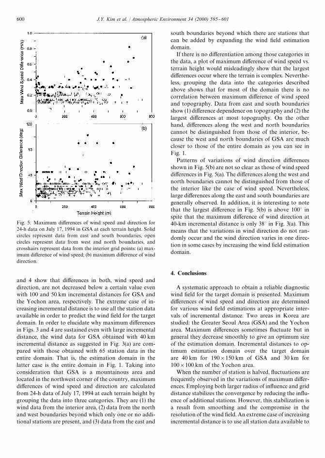
Fig. 5. Maximum di!erences of wind speed and direction for24-h data on July 17, 1994 in GSA at each terrain height. Solidcircles represent data from east and south boundaries, opencircles represent data from west and north boundaries, andcrosshairs represent data from the interior grid points: (a) max-imum di!erence of wind speed; (b) maximum di!erence of winddirection.

and 4 show that di!erences in both, wind speed anddirection, are not decreased below a certain value evenwith 100 and 50 km incremental distances for GSA andthe Yochon area, respectively. The extreme case of in-creasing incremental distance is to use all the station dataavailable in order to predict the wind "eld for the targetdomain. In order to elucidate why maximum di!erencesin Figs. 3 and 4 are sustained even with large incrementaldistance, the wind data for GSA obtained with 40 kmincremental distance as suggested in Fig. 3(a) are com-pared with those obtained with 65 station data in theentire domain. That is, the estimation domain in thelatter case is the entire domain in Fig. 1. Taking intoconsideration that GSA is a mountainous area andlocated in the northwest corner of the country, maximumdi!erences of wind speed and direction are calculatedfrom 24-h data of July 17, 1994 at each terrain height bygrouping the data into three categories. They are (1) thewind data from the interior area, (2) data from the northand west boundaries beyond which only one or no addi-tional stations are present, and (3) data from the east and

south boundaries beyond which there are stations thatcan be added by expanding the wind "eld estimationdomain.

If there is no di!erentiation among those categories inthe data, a plot of maximum di!erence of wind speed vs.terrain height would misleadingly show that the largestdi!erences occur where the terrain is complex. Neverthe-less, grouping the data into the categories describedabove shows that for most of the domain there is nocorrelation between maximum di!erence of wind speedand topography. Data from east and south boundariesshow (1) di!erence dependence on topography and (2) thelargest di!erences at most topography. On the otherhand, di!erences along the west and north boundariescannot be distinguished from those of the interior, be-cause the west and north boundaries of GSA are muchcloser to those of the entire domain as you can see inFig. 1.

Patterns of variations of wind direction di!erencesshown in Fig. 5(b) are not so clear as those of wind speeddi!erences in Fig. 5(a). The di!erences along the west andnorth boundaries cannot be distinguished from those ofthe interior like the case of wind speed. Nevertheless,large di!erences along the east and south boundaries aregenerally observed. In addition, it is interesting to notethat the largest di!erence in Fig. 5(b) is above 1003 inspite that the maximum di!erence of wind direction at40-km incremental distance is only 383 in Fig. 3(a). Thismeans that the variations in wind direction do not ran-domly occur and the wind direction varies in one direc-tion in some cases by increasing the wind "eld estimationdomain.

4. Conclusions

A systematic approach to obtain a reliable diagnosticwind "eld for the target domain is presented. Maximumdi!erences of wind speed and direction are determinedfor various wind "eld estimations at appropriate inter-vals of incremental distance. Two areas in Korea arestudied: the Greater Seoul Area (GSA) and the Yochonarea. Maximum di!erences sometimes #uctuate but ingeneral they decrease smoothly to give an optimum sizeof the estimation domain. Incremental distances to op-timum estimation domain over the target domainare 40 km for 190]150 km of GSA and 30 km for100]100 km of the Yochon area.

When the number of station is halved, #uctuations arefrequently observed in the variations of maximum di!er-ences. Employing both larger radius of in#uence and griddistance stabilizes the convergence by reducing the in#u-ence of additional stations. However, this stabilization isa result from smoothing and the compromise in theresolution of the wind "eld. An extreme case of increasingincremental distance is to use all station data available to

600 J.Y. Kim et al. / Atmospheric Environment 34 (2000) 595}601

estimate the wind "eld of the target domain. When thewind "eld from a limited estimation domain is comparedwith that from all available station data, large di!erencesusually occur along boundaries beyond which there areadditional stations present and where the terrain is high.The former is inevitable as long as a limited size ofdomain and a limited number of stations are employed.Nevertheless, the latter would be alleviated if the complexterrain on the boundary is avoided.

Acknowledgements

This work was supported by the Korea Institute ofScience and Technology and partly also by a grantfrom the IBM Environmental Research Program. Anyopinions, "ndings and conclusions or recommenda-tions expressed in this material are those of the authorsand do not necessarily re#ect the views of the IBMCorporation.

References

Goodin, W.R., McRae, G.J., Seinfeld, J.H., 1980. An objectiveanalysis technique for constructing three-dimensional ur-ban-scale wind "elds. Journal of Applied Meteorology 19,98}108.

Harley, R.A., Russel, A.G., McRae, G.J., Cass, G.R., Seinfeld,J.H., 1993. Photochemical modeling of the Southern Cali-fornia air quality study. Environmental Science and Tech-nology 27, 378}388.

Kumar, N., Russell, A.G., 1996. Comparing prognostic anddiagnostic meteorological "elds and their impacts onphotochemical air quality modeling. Atmospheric Envir-onment 30, 1989}2010.

Seinfeld, J.H., 1988. Ozone air quality models. A critical review.Journal of Air Pollution Research Association 38, 616}645.

Solomon, P.A., 1995. Regional photochemical measurement andmodeling studies : a summary of the air and waste manage-ment association international specialty conference. Journalof Air and Waste Management Association 45, 253}286.

Stephens, J.J., Stitt, J.M., 1970. Optimum in#uence radii forinterpolation with the method of successive corrections.Monthly Weather Review 98, 680}687.

J.Y. Kim et al. / Atmospheric Environment 34 (2000) 595}601 601