Determinants of Stock Market Volatility and Risk Premiamordecai/RiskPremia.pdf · Determinants of...
43
* This research was supported by a grant of the Smith Richardson Foundation to the Stanford Institute for Economic Policy Research (SIEPR). We thank Kenneth Judd for constant advice which was crucial at several points in the development of this work. We also thank Kenneth Arrow, Min Fan, Michael Magill, Carsten Nielsen, Manuel Santos, Nicholas Yannelis, Ho-Mou Wu and Woody Brock for comments on earlier drafts. The RBE model developed in this paper and the associated programs used to compute it are available to the public on Mordecai Kurz’s web page at http://www.stanford.edu/~mordecai. 1 Determinants of Stock Market Volatility and Risk Premia * Mordecai Kurz 1 , Hehui Jin 1 and Maurizio Motolese 2 1 Department of Economics, Serra Street at Galvez, Stanford University, Stanford, CA. 94305-6072, USA 2 Istituto di Politica Economica, Universitá Cattolica di Milano, Via Necchi 5, 20123, Milano, Italy. Received: JUNE 21, 2004 Summary. We show the dynamics of diverse beliefs is the primary propagation mechanism of volatility in asset markets. Hence, we treat the characteristics of the market beliefs as a primary, primitive, explanation of market volatility. We study an economy with stock and riskless bond markets and formulate a financial equilibrium model with diverse and time varying beliefs. Agents’ states of belief play a key role in the market, requiring an endogenous expansion of the state space. To forecast prices agents must forecast market states of belief which are beliefs of “others” hence our equilibrium embodies the Keynes “Beauty Contest.” A “market state of belief” is a vector which uniquely identifies the distribution of conditional probabilities of agents. Restricting beliefs to satisfy the rationality principle of Rational Belief (see Kurz (1994), (1997)) our economy replicates well the empirical record of the (i) moments of the price/dividend ratio, risky stock return, riskless interest rate and the equity premium; (ii) Sharp ratio and the correlation between risky returns and consumption growth; (iii) predictability of stock returns and price/dividend ratio as expressed by: (I) Variance Ratio statistic for long lags, (II) autocorrelation of these variables, and (III) mean reversion of the risky returns and the predictive power of the price/dividend ratio. Also, our model explains the presence of stochastic volatility in asset prices and returns. Two properties of beliefs drive market volatility: (i) rationalizable over confidence implying belief densities with fat tails, and (ii) rationalizable asymmetry in frequencies of bull or bear states. Keywords: Market states of beliefs; market volatility; equity risk premium; riskless rate; over confidence; Heterogenous beliefs; Rational Belief; optimism; pessimism; empirical distribution. JEL Classification Numbers: G1; G12; E43; E44; D58; D84. 1. Introduction The forces which determine equilibrium market volatility and risk premia are probably the most debated topics in the analysis of financial markets. The debate is driven, in part, by empirical evidence of market "anomalies" which have challenged students of the subject. Consumption - based asset pricing theory has had a profound impact on our view of financial markets. Early work of Leroy (1973), Lucas (1978), Breeden (1979), Grossman and Shiller (1981), Mehra and Prescott (1985), Hansen and Singleton (1983) and others show how intertemporal optimization of investor incorporates a subtle relationship between consumption growth and asset returns. However, when examined empirically, this simple relationship fails to provide a correct quantitative measure of risk
Transcript of Determinants of Stock Market Volatility and Risk Premiamordecai/RiskPremia.pdf · Determinants of...

* This research was supported by a grant of the Smith Richardson Foundation to the Stanford Institute for EconomicPolicy Research (SIEPR). We thank Kenneth Judd for constant advice which was crucial at several points in the developmentof this work. We also thank Kenneth Arrow, Min Fan, Michael Magill, Carsten Nielsen, Manuel Santos, Nicholas Yannelis,Ho-Mou Wu and Woody Brock for comments on earlier drafts. The RBE model developed in this paper and the associatedprograms used to compute it are available to the public on Mordecai Kurz’s web page at http://www.stanford.edu/~mordecai.
1
Determinants of Stock Market Volatility and Risk Premia*
Mordecai Kurz1, Hehui Jin1 and Maurizio Motolese2
1Department of Economics, Serra Street at Galvez, Stanford University, Stanford, CA. 94305-6072, USA2Istituto di Politica Economica, Universitá Cattolica di Milano, Via Necchi 5, 20123, Milano, Italy.
Received: JUNE 21, 2004
Summary. We show the dynamics of diverse beliefs is the primary propagation mechanism of volatility in asset markets.Hence, we treat the characteristics of the market beliefs as a primary, primitive, explanation of market volatility. We study aneconomy with stock and riskless bond markets and formulate a financial equilibrium model with diverse and time varying beliefs. Agents’ states of belief play a key role in the market, requiring an endogenous expansion of the state space. To forecast pricesagents must forecast market states of belief which are beliefs of “others” hence our equilibrium embodies the Keynes “BeautyContest.” A “market state of belief” is a vector which uniquely identifies the distribution of conditional probabilities of agents.
Restricting beliefs to satisfy the rationality principle of Rational Belief (see Kurz (1994), (1997)) our economyreplicates well the empirical record of the (i) moments of the price/dividend ratio, risky stock return, riskless interest rate and theequity premium; (ii) Sharp ratio and the correlation between risky returns and consumption growth; (iii) predictability of stockreturns and price/dividend ratio as expressed by: (I) Variance Ratio statistic for long lags, (II) autocorrelation of these variables,and (III) mean reversion of the risky returns and the predictive power of the price/dividend ratio. Also, our model explains thepresence of stochastic volatility in asset prices and returns. Two properties of beliefs drive market volatility: (i) rationalizableover confidence implying belief densities with fat tails, and (ii) rationalizable asymmetry in frequencies of bull or bear states.
Keywords: Market states of beliefs; market volatility; equity risk premium; riskless rate; over confidence;Heterogenous beliefs; Rational Belief; optimism; pessimism; empirical distribution. JEL Classification Numbers: G1; G12; E43; E44; D58; D84.
1. Introduction
The forces which determine equilibrium market volatility and risk premia are probably the
most debated topics in the analysis of financial markets. The debate is driven, in part, by empirical
evidence of market "anomalies" which have challenged students of the subject. Consumption -
based asset pricing theory has had a profound impact on our view of financial markets. Early work
of Leroy (1973), Lucas (1978), Breeden (1979), Grossman and Shiller (1981), Mehra and Prescott
(1985), Hansen and Singleton (1983) and others show how intertemporal optimization of investor
incorporates a subtle relationship between consumption growth and asset returns. However, when
examined empirically, this simple relationship fails to provide a correct quantitative measure of risk

2
premia. The Equity Premium Puzzle (see, Mehra and Prescott (1985)) is a special case of the fact
that assets prices are more volatile than can be explained by "fundamental" shocks.
Difficult to account for risk premia are not confined to the consumption based asset pricing
theory; they arise in many asset pricing models. Three examples will illustrate. The Expectations
Hypothesis is rejected by most studies of the term structure (e.g. Backus, Gregory and Zin (1989),
Campbell and Shiller (1991)) implying excessive risk premium on longer maturity debt. Foreign
exchange markets exhibit a "Forward Discount Bias" (see Froot and Frankel (1989) and Engel
(1996)) implying an unaccounted for risk premium for holding foreign exchange. The pricing of
derivatives generates excess implied volatility of underlying securities, resulting in unaccounted for
risk premia. Some treat these as unusual anomalies and give them distinct labels, presuming
standard models of asset pricing can account for all normal premia. Our perspective is different.
We suggest market volatility and risk premia are primarily determined by the structure of
agents’ expectations called "market state of belief." Diversity and dynamics of beliefs are then the
root cause of price volatility and the key factor explaining risk premia. Agents may be "bulls" or
"bears." A bull at date t expects the date t+1 rate of return on investments to be higher than normal,
where "normal" is defined by the empirical distribution of past returns. Date t bears expect returns
at t+1 to be lower than normal. Agents do not hold Rational Expectations (in short RE) since the
environment is dynamically changing, non stationary, and true probabilities are unknown to anyone.
In such complex environment agents use subjective models. Some consider these agents irrational,
but one cannot require them to know what they cannot know: there is a wide gulf between an RE
agent and irrational behavior. We explore the structure of economies with diverse beliefs and show
they must have an expanded state space. Our computing models assume agents hold rational beliefs
in accord with the theory of Rational Belief Equilibrium (in short, RBE) due to Kurz (1994) and
explored in Kurz (1996),(1997). This rationality principle strikes a proper balance between RE and
irrational behavior. To assist readers unfamiliar with this theory, we briefly explain it.
The Rational Belief Principle. “Rational Belief” (in short, RB) is not a theory that demonstrates
rational agents should adopt any particular belief. Indeed, since the RB theory explains the
observed belief heterogeneity, it would be a contradiction to propose that a particular belief is the
“correct” belief agents should adopt. The RB theory starts by observing that the true stochastic law

3
of motion of the economy is non-stationary with structural breaks and complex dynamics hence the
probability law of the process is not known. Agents have a long history of past data generated by
the process which they use to compute relative frequencies of finite dimensional events hence all
finite moments. With this knowledge they compute the empirical distribution and use it to construct
an empirical probability measure over sequences. Kurz (1994) shows the estimated probability
model is stationary and hence it is called the “empirical measure” or the “stationary measure.”
In contrast with a Rational Expectations Equilibrium (in short, REE) where the true law of
motion is known, agents in an RBE who do not know the truth, form subjective beliefs based only
on observed data. Hence, any principle on the basis of which agents can be judged as rational must
be based only on the data. Since a “belief” is a model of the economy together with a probability
over sequences of variables, it can be used to generate artificial data. With simulated data an agent
can compute the empirical distribution of observed variables. The RB theory then proposes a
simple Principle of Rationality. It says that if an agent’s model generates an empirical distribution
which is not the same as the one known for the economy, then the agent’s model (i.e. “belief”) is
irrational. The RB rationality declares a belief to be rational only if it is a model which cannot be
disproved with the empirical evidence. Since diverse theories are compatible with the evidence, this
rationality principle allows diversity of beliefs among equally informed rational agents. For agents
holding RB date t theoretical moments may deviate from the empirical moments but the RB
rationality principle requires the time average of all theoretical moments to equal the empirical
moments. In particular, date t forecasts may deviate from empirical forecasts but the time average
of all forecasts must agree with the empirical forecasts. It follows as a theorem that agents who
hold rational beliefs must have forecast functions which vary over time. The tool we use to
describe the beliefs of agents is the “market state of belief.” It is explained in details in this paper.
The RB rationality is compatible with several known theories. An REE is a special case of
an RBE. Most models of Bayesian learning satisfy the RB rationality principle. Also, several
models of Behavioral Economics satisfy this principle for some parameter values.
Earlier papers using the RBE rationality principle have also argued that agents’ beliefs are
central to explaining market volatility (e.g. Kurz (1996), (1997a), Kurz and Schneider (1996), Kurz
and Beltratti (1997), Kurz and Motolese (2001), Kurz and Wu (1996) and Nielsen (1996)). These
4
papers aimed to explain a list of financial "anomalies." (for a unified treatment see Kurz and
Motolese (2001)). The RBE theory was used by Kurz (1997b) and Nielsen (2003) to explain the
volatility of foreign exchange rates. These papers used OLG models where exogenous shocks are
discrete and agents have a finite set of belief states. Wu and Guo (2003) (2004) study speculation
and trading in the steady state of an infinite horizon model. This paper’s contribution consists of
four parts: (i) ours is an infinite horizon model, (ii) all random variables are continuous, (iii) AR(1)
processes describe beliefs and exogenous shocks, and (iv) we explicitly model agents’ beliefs about
the market state of belief, which are beliefs about the beliefs of others. We argue that this is the
crucial property needed for understanding the volatility and risk premia in financial markets.
The Main Results . First, "Belief states" are developed as a tool for equilibria with diverse belief.
Next, our method is to use properties of market beliefs as primitive explanation of volatility. Two
characteristics of beliefs fully account for all features of volatility and premia observed in markets:
(A) high intensity of fat tails in the belief densities of agents;
(B) asymmetry in the proportion of bull and bear states in the market over time.
High intensity means agents exhibit rationalizable over confidence with fat tails in their subjective
densities. Asymmetry in frequency of belief is a characteristic which says that on average, at more
than half of the time agents do not expect to make excess returns. Our model also implies market
returns must exhibit stochastic volatility which is generated by the dynamics of market belief.
2. The Economic Environment
The economy has two types of agents and a large number of identical agents within each
type. An agent is a member of one of the two types of infinitely lived dynasties identified by their
endowment , utility ( defined over consumption) and by their belief. A dynasty member lives a fixed
short life and during his life makes decisions based on his own belief without knowing the states of
belief of his predecessors. He is replaced by an identical member. There are two assets: a stock
and a riskless, one period, bond. There is an aggregate output process which isYt , t'1, 2, . . .
divided between dividends paid to owners of the common stocks and non -Dt , t'1, 2, . . .
dividend endowment which is paid to the agents. The dividend process is described by

1A Stable Process is defined in Kurz (1994). It is a stochastic process which has an empirical distribution of theobservable variables defined by the limits of relative frequencies of finite dimensional events. These limits are used to definethe empirical distribution which, in turn, induces a probability measure over infinite sequences of observables which we referto as the “stationary measure” or the “empirical measure.” A general definition and existence of this probability measure isgiven in Kurz (1994), (1997) or Kurz-Motolese (2001) where it is shown that this probability must be stationary. Statementsin the text about “the stationary measure” or “the empirical distribution” is always a reference to this probability. Its centralityarises from the fact that it is derived from public information and hence the stationary measure is known to all agents andagreed upon by all to reflect the empirical distribution of observable equilibrium variables.
2 The key assumption is then that agents do not know the true probability but have ample past data from which theydeduce that (2) is implied by the empirical distribution. Hence the data reveals a memory of length 1 and residuals which arei.i.d. normal. This assumption means that even if (2) is the true data generating process, agents do not know this fact. Anagent may believe the true process is non-stationary and different from (2) and then build his subjective model of the market.
5
(1) Dt%1 ' Dt ext%1
where , t = 1, 2, ... is a stochastic process under a true probability which is non-stationary withxt
structural breaks and time dependent distribution. This time varying probability is not known by
any agent and is not specified. Instead, we assume , t = 1, 2, ... is a stable process1 hence it hasxt
an empirical distribution which is known to all agents who learn it from the data. This empirical
distribution is represented by a stationary Markov process, with a year as a unit of time, defined by2
(2) with i.i.d.xt%1 ' (1 & λx) x (
% λxxt % ρxt%1 ρ
xt%1 - N( 0 , σ2
x )
The infinitely lived agents are enumerated j = 1, 2 and we use the following notation:
- consumption of j at t; C jt
- amount of stock purchased by j at t; θjt
- amount of one period bond purchased at discount by agent j at t;B jt
- stock price at date t;qst
- the discount price of a one period bond at t;qbt
- non capital income of agent j at date t;Λjt
Ht - information at t, recording the history of all observables up to t.
Given probability belief , agent j selects portfolio and consumption plans to solve the problemQ jt
(3a) Max(C j,θj ,B j)
EQ j [j4
t '0
βt 11 & γ
( C jt )1 & γ | Ht ]
subject to:
(3b) .C jt % qs
t θjt % q b
t B jt ' Λ
jt % ( qs
t % Dt )θjt&1 % B j
t&1
We assume additively separable, power utility over consumption, a model that failed to generate
premia in other studies (see, Campbell and Cochrane (2000)). We focus on diverse beliefs hence

6
assume the two utility functions are the same. Introduce the normalization for j = 1, 2
.ωjt /
Λjt
Dt
, c jt /
C jt
Dt
, q st /
qst
Dt
, b jt /
B jt
DtWith this normalization the budget constraint becomes
(3b’) .c jt % q s
t θjt % q b
t b jt ' ω
jt % (q s
t % 1)θjt&1 % b j
t&1 e&xt
The Euler equations are
(4a) (c jt )&γq s
t ' βEQ jt[ ( c j
t%1 )&γ (1 % q st%1 )e
(1 & γ )xt%1 | Ht ]
(4b) (c jt )&γq b
t ' βEQ jt[ ( c j
t%1 )&γ e&γxt%1 | Ht ]
and the market clearing conditions are then
(4c) θ1t % θ
2t ' 1
(4d) .b 1t % b 2
t ' 0
3. A Rational Expectations Equilibrium (REE)
Strictly speaking we cannot evaluate the REE since the true output process has not been
specified. We thus define an REE to be the economy in which all agents believe that (2) is the true
output process. To evaluate the volatility of this REE in an annual model we specify parameters of
(2). Unfortunately, different estimates of the parameter values are available, depending upon time
span of data, unit of time (annual vs. quarterly) and definition of terms (see, for a sample, Backus,
Gregory and Zin (1989), Campbell (2000) and Rodriguez (2002) Appendix 2, based on Shiller in
(http://www.econ.yale.edu/shiller)). We use the annual estimates in Campbell (2000) Table 3, which
are consistent with Mehra and Prescott (1984). Hence, for the rest of this paper we set , β'0.96
, and , all within the empirically estimated range. γ'2.00 , x (
'0.01773 λx ' &0.117 σx ' 0.03256
Ours is a theoretical paper aiming to draw qualitative conclusions. We use realistic parameter values
since we wish our simulations to result in numerical values which are close to the observed data. For
simplicity we assume , a constant hence total resources, or GNP, equal (1+2T)Dt and theωjt ' ω
Dividend/GNP ratio is . As we model only income from publically traded stocks, the11 % 2ω
Dividend/(Household Income) ratio should include corporate dividends but exclude self employed
income and imputed income from other asset categories. This ratio is about 15% (see survey data in
Heaton and Lucas (1996)) hence we select . This fact has very little effect on the results.ωjt ' 3
We simulated this REE and report in Table 1 the mean and standard deviations of (i) the

3 Other approaches to the equity premium puzzle were reported by Brennan and Xia [1998], Epstein and Zin [1990],Cecchetti, Lam and Mark [1990],[1993], Heaton and Lucas [1996], Mankiw [1986], Reitz [1988], Weil [1989] and others. Formore details see Kocherlakota [1996]. Some degree of excess volatility can also be explained with explicit learning mechanismwhich does not die out (see for example Timmermann (1996)).
4 Campbell and Cochrane (1999), (2000) assume that at habit the marginal utility of consumption and degree of risk
aversion rise without bound. Hence, when consumption declines to habit, risk aversion increases, stock prices decline and risk
premium rises. Although the model generates moments which are closer to those observed in the market, the theory is
unsatisfactory. First, with Xt = habit, utility is . But why should the marginal utility and risk aversion explode11&γ
(Ct&Xt)1&γ
when Ct approaches the mean of past consumption? Campbell and Cochrane (1999, page 244) show that for the model to
generate the desired moments, the degree of risk aversion is 80 at steady state and exceeds 300 frequently along any time path.
If instead we use Abel’s (1990), (1999) formulation , marginal utility is normalized to be 1 at habit but the model11&γ
(Ct
Xt
)1&γ
does not generate volatility. Second, big fluctuations of stock prices are observed during long periods when consumption
grows smoothly as was the case during the volatile period of 1992 - 2002. Finally, the model predicts perfect correlation
between consumption growth and stock returns but the record (see Table 1) shows date t stock returns have low correlation
with date t consumption growth. Above all, the habit formation model proposes a theory which claims that asset premia are
caused by an unreasonably high degree of risk aversion. This is not credible.
7
price\dividend ratio , (ii) the risky return R, (iii) the riskless rate ; the equity premium , theq s ep
Sharp Ratio and the correlation between x and R. Moments of market data vary with sources
reporting and methods of estimation. The market data reported in Table 1 are based on Shiller
(http://www.econ.yale.edu/shiller) and others. The results are familiar. Note that apart from the low
equity premium, the REE volatility measures are lower than market data by an order of magnitude.
The "Equity Premium" is not the only puzzle; the wider question is how to explain market volatility.
Table 1: Simulated Moments Of Key Variables In REE(all moments are annualized)
R q sσq s σR r σr ep ρRx shrp
Model Data 16.71 0 .055 7.94% 3.78% 7.70% 0.79% 0.24% 0.995 0.064
Market Data 25 7.1 7% 18.00% 1.00% 5.70% 6.00% 0.100 0.333
Some have argued in favor of introducing habit formation in utility in order to generate time
variability of risk aversion (e.g. see Abel (1990), (1999), Constantinides (1990), Campbell and
Cochrane (1999), (2000)3). We are not persuaded by this model since habit formation can explain
the equity premium only if it assumes unreasonably high degree of risk aversion4. Our alternative
view proposes that risk premia are determined primarily by the structure of market expectations.
Our argument is developed in sections 4, 5 and 6. First, in Section 4 we develop the general
structure of equilibria where agents have time varying and diverse beliefs. These ideas apply to any

8
model with diverse beliefs, not only to a Rational Belief framework. We then explain the restrictions
which the RB principle impose on the model and in Sections 5 and 6 we develop the main results.
4. The General Structure of Equilibria with Diverse and Time Dependent Beliefs
Although (2) represent moments of past data, agents believe the economy is not stationary
and past data do not provide adequate guide to the future. With technology and institutional changes,
agents do not believe a fixed stationary model captures the complexity of society. Hence, they may
not agree on a “correct” model that generated this empirical evidence. Indeed, we would expect that
different agents using the same evidence will come up with different theories to explain the data and
hence with different models to forecast prices. Each investor may have his own model of market
dynamics. But then, one may ask, what are the specific formal belief formation models agent use to
deviate from the empirical forecasts and why do they select these models? Since agents do not hold
RE, how do they rationalize their beliefs? These are questions which we cannot fully address here.
Our methodology is to use the distribution of beliefs to explain market volatility hence we need to
determine a level of detail at which agents “justify” their beliefs. If we aim at a complete specification
of such modeling, our study is doomed to be bogged down in details of inference from small samples
and information processing. Although interesting, from a general equilibrium perspective it is not
needed. To study volatility we focus on a narrow but operational question. Since (4a)-(4b) require
specification of conditional probabilities, we need only a tractable way to describe differences among
agents’ beliefs and time variability of their conditional probabilities, without fully specified models to
justify them. From our point of view what matters is the fact that market beliefs are diverse and time
dependent; the reasoning which lead agents to the subjective models are secondary. The tool we
developed for this goal is the individual and the market “state of belief” which we now explain.
4.1 Market States of Belief and Anonymity: Expansion of the State Space
The usual state space for agent j is denoted by S j but when beliefs change over time we
introduce an additional state variable called “agent j state of belief .” It is a variable generated by
agent j, expressing his date t subjective view of the future and denoted by . It has theg jt 0 G j
property that once specified, the conditional probability function of an agent is uniquely specified and

5 Note that larger values of g imply a more bearish perspective. In the applications below larger g will express anagent’s reduced probability belief in making excess returns. This may appear unnatural but we study equilibria withasymmetry measured by the frequency at which an agent is a bull or a bear. One of our main results says that the data supportsa model where, on average, agents expect to make excess returns less than 50% of the time or, equivalently, that in a largemarket a majority of agents are pessimistic about making excess returns. We thus focus on the market pessimists. Since in thecomputational model we use a logistic function to express this asymmetry, it turns out that the use of a logistic functionnecessitates the condition that a larger g means more bearishness. Without the desired asymmetry g could have an oppositeinterpretation. We discuss this point further in Appendix A.
9
hence has the form . Changes in j’s conditional probability function are pinnedPr(s jt%1 , g j
t%1 | s jt , g j
t )
down by j’s state of belief; is actually a proxy for j’s conditional probability function. We noteg jt
that are privately perceived by agent j and have meaning only to him. Since a dynasty consists ofg jt
a sequence of decision makers, used by j has no impact on the description of beliefs by otherg jt
dynasty members. In the model of this paper agents forecast dividend or profit growth rate xt+1 (i.e.
the exogenous variable) hence describes agent j conditional probability of profit growth at g jt 0 ú
t+1. We shall permit rational agents to be “bulls” who are optimistic about future excess returns or
“bears” who are pessimistic about future excess returns. To understand the role of we introduceg jt
later a reference parameter a and then interpret in the following way:g jt
• If agent j agrees with the empirical distribution and makes profit growth forecasts ing jt ' a
accord with (2);
• If agent j disagrees with the empirical distribution. If he is a bear and makesg jt … a g j
t > a
lower profit growth forecasts than the ones implied by (2); if he is a bull and makesg jt < a
higher profit growth forecasts than the ones implied by (2)5.
As indicated, we do not explain the reasoning used by agents to deviate from the empirical
forecast. It is a common practice among forecasters to use the strict econometric forecast only as a
benchmark. Given such benchmark, a forecaster uses his own model to add a component reflecting
an evaluation of circumstances at a date t that call for a deviation at t from the benchmark. In short,
is a description of how the model of agent j deviates from the statistical forecast implied by (2). g jt
In this paper we assume that at any date the state of belief is a realization of a process of the form
(5) .g jt%1 ' λzg j
t % λzjx (xt & x () % ρ
g j
t%1 , ρg j
t%1 - N( 0 , σ2
g j )
Persistent states of belief which depends upon current market data fit different cases of economies
with diverse beliefs. We consider three examples to illustrate how one may think about them.

6 See Woodford (2003) , Morris and Shin (2002), Allen Morris and Shin (2003) and others
10
(i) Measure of Animal Spirit. “Animal Spirit” expresses intensity at which agents carry out
investments and this, in turn, is based upon expected rewards. identifies the probability an agentg jt
assigns to high or low rates of return hence can be interpreted as a measure of “animal spirit.”g jt
(ii) Learning Unknown Parameters. In a learning context agents use prior distributions on unknown
parameters. Since defines an agent’s belief about the profit growth process we can identify asg jt g j
t
a posterior parameter of its mean value function. A posterior as a linear function of the prior and
current data is familiar. We add to reflect changes in priors over time due to regime shifts andρg j
t%1
changes in structure. Among such changes are decision makers in the dynasty who are replaced by
successors who select new priors. Infinite horizon is a proxy for a sequence of decision makers in a
changing economy. With diverse beliefs, models a diversity of beliefs over time.ρg j
t%1
(iii) Privately generated subjective sunspot to depend upon real variables. may play the role of ag jt
private sunspot with three properties (a) an agent generates his own under a marginal distributiong jt
known only to him, (b) it is not observed by other agents, and (c) it’s distribution may depend upon
real variables. Also, the correlation across agents is a market externality, not known to anyone.
Under this interpretation is a major extension of the common concept of a “sunspot” variable.g jt
In equilibria with diverse beliefs agents’ decision rules are functions of hence equilibriumg jt
prices depend upon , the agents’ conditional probabilities. But then, should j begt' (g 1t ,g 2
t , . . . ,g Nt )
allowed to recognize his is the jth coordinate of and thus give him some market power? Theg jt gt
principle of anonymity introduced in Kurz, Jin and Motolese (2003a), (2003b) requires competitive
agents to assume they cannot affect endogenous variables. It is analogous to requiring a competitive
firm to assume it has no effect on prices. The issue here is the specification of how agents forecast
prices. To that end we define the “market state of belief “ as a vector , keeping inzt' (z 1t , z 2
t , . . . , z Nt )
mind the model consistency condition which is not recognized by agents. This makes marketzt'gt
state of belief a macroeconomic state variable and equilibrium prices actually become functions of zt
and not functions of . Agent j views as “market belief” and as unrelated to him since it is thegt zt
belief of other agents. In small economies prices depend upon the distribution zt' (z 1t , z 2
t , . . . , z Nt )
but in many applications only a few moments matter. In some models of diverse beliefs writers focus
only on the average, and define the market state of belief by the mean belief 6 . Anonymityzt'1Nj
N
j'1z j
t
7 Allen, Morris and Shin (2003) seem to suggest the Beauty Contest is associated with the failure of the marketbelief to satisfy the law of iterated expectations (see title of their paper). It is clear the average market probability beliefs doesnot satisfy the law of iterated expectations since the average conditional probability is not a proper conditional probability.However, this fact is independent of the problem defined by the Keynes Beauty Contest which requires agents in an economywith diverse beliefs to forecast the future average market state of belief.
11
is so central to our approach that we use three notational devices to highlight it:
(i) denotes the state of belief of j as known by the agent only. g jt
(ii) denotes market state of belief, observed by all. Competitive behavior means jzt' (z 1t , z 2
t , . . . , z Nt )
does not associate with although is a model consistency condition. g jt zt g j
t ' z jt
(iii) is agent j’s forecast of the market state of belief at future date t+1.z jt%1' (z j1
t%1 ,z j2t%1 , . . . , z jN
t%1)
The introduction of individual and market states of belief has two central implications:
(A) The economy has an expanded state space, including market belief . in thiszt zt' ( z 1t , z 2
t )0ú2
paper. Hence diverse beliefs create new uncertainty which is the uncertainty of what others may do.
This adds a component of volatility which cannot be explained by “fundamental” shocks. Denoting
usual state variables by , the price process , t = 1, 2, ... is defined by a map likest (q st , q b
t )
(6) .qs
t
qbt
' Ξ( st , z 1t , z 2
t , . . . , z Nt )
Our equilibrium is thus an incomplete Radner (1972) equilibrium with an expanded state space.
(B) To forecast prices agents must forecast market beliefs. Although all use (6) to forecast prices,
agents’ forecasts are different since each forecasts given his own state . This is a(st%1 , zt%1) g jt
feature of the Keynes Beauty Contest: to forecast equilibrium prices you must forecast beliefs of
other agents. A Beauty Contest does not entail higher order of beliefs: at t you form belief about
market belief but the date t+1 market belief is not a probability about your date t belief state7. zt%1
We now return to the economy with two agent types and simplify by assuming the market
belief is observable. This assumption is entirely reasonable since there is a vast amount of(z 1t , z 2
t )
public data on the distribution of forecasts in the market and on the dynamics of this distribution.
Indeed, using forecast data obtained from the Blue Chip Economic Indicators and the Survey of
Professional Forecasters we constructed various measures of market states of belief. Since (z 1t , z 2
t )
is observable we need to modify the empirical distribution (2) and include in it. We assume(z 1t , z 2
t )

12
the empirical distribution of profit growth and the states of belief is an AR process of the form
(7a) xt%1 ' (1 & λx)x (
% λx xt % ρxt%1
(7b) , z 1t%1 ' λz 1z
1t % λ
z 1
x (xt & x () % ρz 1
t%1
ρxt%1
ρz 1
t%1
ρz 2
t%1
- N
0
0
0
,
σ2x, 0, 0
0, 1, σz 1z 2
0, σz 1z 2, 1
' Σ , i.i.d.
(7c) z 2t%1 ' λz 2z
2t % λ
z 2
x (xt & x () % ρz 2
t%1
In any application one assumes the parameters of (7a)-(7c) are known by all. With regard to x, we
have set values for in Section 2. We normalize by setting variances of equal to 1. (λx , x ( , σx) ρz j
t%1
To specify parameters of the zj equations recall that z measures how optimistic agents are about
future returns on investment. With this in mind we used forecasts reported by the Blue Chip
Economic Indicators and the Survey of Professional Forecasters, and “purged” them of observables.
We then estimated principal components to handle multitude of forecasted variables (for details, see
Fan (2003)). The extracted indexes of beliefs imply regression coefficients around 0.5 - 0.8 hence
we set . Investors’ forecasts of financial variables such as corporate profits, are highlyλz 1'λz 2'0.7
correlated and a value of is realistic. In this paper we study only symmetric economiesσz 1z 2 ' 0.90
where agents differ only in their beliefs hence we assume . The evidence shows thatλz 1
x ' λz 2
x ' λzx
positive profit shocks lead agents to revise upward their economic growth forecasts implying . λzx > 0
Our best guess of this parameter leads us to set but we discuss it again later. λzx ' 0.9
To write (7a) -(7c) in a more compact notation let , wt ' ( xt & x ( , z 1t , z 2
t ) ρt ' (ρxt , ρz 1
t , ρz 2
t )
and denote by A the 3×3 matrix of parameters in (7a) -(7c). We then write (7a) -(7c) as
(8) .wt%1 ' Awt % ρt%1 , ρt%1 - N( 0 , Σ )
Denote by V the 3×3 unconditional covariance of w defined by . We use theV ' Em( wwN )
value of V and compute it here as a solution of the equation
(9) .V ' AVAN % Σ
Finally, denote by m the probability measure on infinite sequences implied by (8) with the invariant
distribution as the initial distribution. We then write where Ht is the history at t. Em( wt%1 |Ht) ' Awt
To complete the description of an equilibrium we need to specify the individual beliefs. However, we
stress that the description to follow is general, applying to any model with diverse beliefs.
4.2 The General Structure of Beliefs and the Problem of Parameters
A perception model is a set of transition functions of state variables, expressing an agent’s

13
belief about date t+1 conditional probability. We first explain the general form of a perception model,
and provide details later. Let be date t+1 variables as perceived by j and letw jt%1 ' (x j
t%1 ,z 1jt%1 ,z 2j
t%1 )
be a 3 dimensional vector of date t+1 random variables conditional upon . Ψt%1(gj
t ) g jt
Definition 1: A perception model in the economy under study has the general form
(9a) together with (5).w jt%1 ' Awt % Ψt%1( g j
t )
Since , we write (9a) in the simpler formEm( wt%1 | Ht) ' Awt
(9b) .w jt%1 & Em( wt%1 | Ht) ' Ψt%1(g j
t )
(9b) reveals that is j’s deviation in forecasting from . In general weE j[Ψt%1|gj
t ] w jt%1 Em( wt%1 | Ht)
have and the mean of the agent’s forecast changes with . If as inE j[Ψt%1|gj
t ] … 0 g jt Ψt%1(g j
t ) ' ρt%1
(8), j uses the empirical probability m as his belief. Condition (9b) shows that we model Ψt%1(gj
t )
so that agents may be over-confident by being optimistic or pessimistic relative to the empirical
forecasts. We now postulate a random variable with which we model simply byηjt%1(g j
t ) Ψt%1(gj
t )
(10) Ψt%1(g jt ) '
λxgη
jt%1 (g j
t ) % ρx j
t%1
λz1g η
jt%1 (g j
t ) % ρz j1
t%1
λz2g η
jt%1 (g j
t ) % ρz j2
t%1
, ρjt%1 - N(0 , Ωj
ρρ) i.i.d.
where . By (9a) a perception model includes as a fourth dimension withρjt%1 ' ( ρx j
t%1 , ρz j1
t%1 , ρz j2
t%1 ) g jt%1
an innovation and a covariance matrix denoted by , reflecting the vector ρjt%1 Ωj r i
j ' Cov(w i , g j )
for i = 1, 2, 3. For simplicity we use only one random variable to define all components ofηjt%1(g j
t )
. In addition, we study only symmetric markets where agents differ at any t only in twoΨt%1(gj
t )
respects: they may have different date t states of belief and different portfolios due to difference in
histories. Hence, we assume are common to both agents. These describe how anλg ' (λxg , λz1
g , λz2g )
agent’s forecasts vary with his beliefs. To specify agents’ beliefs in any particular model one needs to
specify , and for i = 1, 2, 3. Combining all these partsΨt%1(gj
t ) λg ' (λxg , λz1
g , λz2g ) r i
j ' Cov(w i , g j )
we can formulate the final form of the perception models of agent j:
(11a) x jt%1 ' (1 & λx)x (
% λx xt % λxgη
jt%1(g j
t ) % ρx j
t%1
(11b) z j1t%1 ' λzz 1
t % λzx (xt & x () % λ
zgη
jt%1(g j
t ) % ρz j1
t%1
(11c) z j2t%1 ' λzz 2
t % λzx (xt & x () % λ
zgη
jt%1(g j
t ) % ρz j2
t%1

14
(11d) .g jt%1 ' λz g j
t % λzx ( xt & x () % ρ
g j
t%1
is i.i.d. Normal with mean zero and covariance matrix of the formρjt%1' (ρx j
t%1 , ρz j1
t%1 , ρz j2
t%1 , ρg j
t%1) Ωj
(11e) .Ωj'
Ωjρρ
, Ωwg j
ΩN
wg j , σ2
g j
where = . Note two facts. First , Ωwg j [Cov( ρxt%1 , ρg j
t%1 ) , Cov( ρz 1
t%1 , ρg j
t%1 ) , Cov( ρz 2
t%1 , ρg j
t%1 )] λxgη
jt%1( g j
t )
in the first equation reflects diverse beliefs about profit shocks. The agent’s forecast of isx jt%1
, not as in (7a). The term EQ jt( x j
t%1&x () ' λx( xt&x ()%λxgEQ j
tη
jt%1(g
jt ) λx(xt&x () λ
xgEQ j
tη
jt%1(g
jt )
measures the agent’s forecast deviation from (7a). Second, in the second(λzgη
jt%1( g j
t ) , λzgη
jt%1( g j
t ) )
and third equations measure the effect of j’s belief on his forecast of the belief of others at(z j1t%1 , z j2
t%1)
t+1. Since prices depend on , the terms and contribute to diversity of (z 1t%1 , z 2
t%1) λzgη
jt%1(g
jt ) λ
zgη
jt%1(g
jt )
t+1 price forecasts. These are the key forces which generate market volatility.
(11a)-(11e) show that given the assumed symmetry, the case of λg ' (λxg , λz1
g , λz2g ) ' (0 ,0 ,0 )
fully characterizes an economy where all agents believe the empirical distribution is the truth. This
case has the essential property of an REE since there is no diversity of beliefs. In such an economy
the volatility of equilibrium quantities is determined only by the volatility of xt in (2).
Summary of Belief Parameters Given symmetry, parameters specifying belief of j are then
and parameters defining the variable explained next. A theory with unrestricted(λg , Ωj ) ηjt%1(g j
t )
beliefs would specify these parameters and some may consider it to be Bounded Rationality. Our
models below assume agents satisfy the RB rationality conditions and we explain in Section 4.4 the
restrictions imposed by RB. Note that anonymity requires the idiosyncratic component of an agent’s
belief not to be correlated with market beliefs. This is translated to the requirement that
Ωz 1g j ' Cov( ρz 1
t%1 , ρg j
t%1 ) ' 0
.Ωz 2g j ' Cov( ρz 2
t%1 , ρg j
t%1) ' 0
Hence, anonymity restricts two components of even in a theory without restrictions on belief.Ωwg j
4.3 Modeling Tractable and Computable Functions Ψt%1(gj
t )
We model so as to permit agents to be over confident by assigning to some eventsΨt%1(gj
t )
higher probability than the empirical frequency. Evidence from the psychological literature (e.g.
Svenson (1981), Camerer and Lovallo (1999) and references) shows agents exhibit such behavior. In
15
some cases this behavior may be irrational but this is not generally true. Institutional and technical
changes are central to an economy and past statistics do not provide the best forecasts for the
future. Deviations from empirical frequencies reflect views based on limited recent data about
changed conditions. Agents have financial incentive to make such judgments since major financial
gains are available to those who bet on the correct market changes. We now discuss the
asymmetries built into modeling .Ψt%1(gj
t )
Asymmetry and Intensity of Fat Tails in . Asymmetry and "fat" tails, reflecting overΨt%1(gj
t )
confidence, is introduced into the computational model through . We define by itsηjt%1(g
jt ) η
jt%1(g
jt )
density, conditional on , as a step function g jt
(12) p(ηjt%1 |g j ) '
φ1( g j ) f(ηjt%1 ) if η
jt%1 $ 0
φ2( g j ) f(ηjt%1 ) if η
jt%1 < 0
where and (in (10)) are independent and where . The functionsηjt%1 ρ
g j
t%1 f(η) ' [1/ 2π] e&
η2
2
are defined by a logistic function with two parameters a and b(φ1(g) ,φ2(g) )
(13) , and define , φ ( g j ) ' 1
1%e b(g j&a)
G / Egφ (g j )
(14) a < 0 , b < 0 and . φ1 ( g j ) 'φ( g j )
G, φ2 ( g j ) ' 2 & φ1 (g j)
The parameter a measures asymmetry and the parameter b measures intensity of fat tails in
beliefs. Details of this construction and the implied moments are discussed in Appendix A.
To explain (12)-(14), note that for large, goes to one, implying that g jt φ ( g j ) φ1 ( g j )
goes to 1/G. Hence, by (12) large > a implies high probability that . Similarly, smallg jt η
jt%1 > 0
< a implies high probability that . To interpret what > a means requires a modelg jt η
jt%1 < 0 g j
t
convention. A convention must specify what means and this depends upon . In anηjt%1 > 0 Ψt%1(g
jt )
economy with , raises j’s forecast of but in an economy with , λxg>0 η
jt%1 > 0 x j
t%1 λxg<0 η
jt%1 > 0
lowers j’s forecast of . We have thus motivated a formal definition of bull and bear states:x jt%1
Definition 2: Let be the probability belief of agent j. Then is said to be Q j g jt
a bear state for agent j if ;EQ j[xj
t%1 |g jt ,Ht] < Em(xt%1 |Ht)
16
a bull state for agent j if .EQ j[xj
t%1 |g jt ,Ht] > Em(xt%1 |Ht)
Now recall that . From (12) we know (see Appendix A forx jt%1' (1&λx)x (
%λx xt%λxgη
jt%1(g j
t )% ρx j
t%1
detail) that if > a then hence we have two cases. If then > ag jt Ej[η
jt%1 (g j
t ) | g jt ] > 0 λ
xg < 0 g j
t
means agent j is in a bear state and expects profit growth below normal at date t+1. Since a < 0
this also means that bear states occur with frequency higher than 50%. If then > a meansλxg > 0 g j
t
agent j is in a bull state and is optimistic about t+1 profit growth being above normal. Again, since
a < 0 this also implies that bull states occur with frequency higher than 50%. “Normal” is defined
relative to the empirical forecast. In sum, we have two basic economies:
Economy 1: for all agents and bear states are more frequent, henceλxg < 0
> a means agent j is pessimistic about profit growth and excess stock returns at t+1g jt
< a means agent j is optimistic about profit growth and excess stock returns at t+1.g jt
Economy 2: for all agents and bull states are more frequent, henceλxg > 0
> a means agent j is optimistic about profit growth and excess stock returns at t+1g jt
< a means agent j is pessimistic about profit growth and excess stock returns at t+1.g jt
What are the beliefs in bull and bear states? Consider Economy I. As increase,(g jt &a)
rises and declines. Hence when > a an agent increases the positive part of aφ1(gj
t ) φ2(gj
t ) g jt
normal density in (12) by a factor and decreases the negative part by . Whenφ1(gj
t ) > 1 φ2(gj
t ) < 1
the opposite occurs: the negative part is shifted up by and the positive part isg jt < a φ2(g
jt ) > 1
shifted down by . The amplifications are defined by gj, by a and byφ1(gj
t ) < 1 (φ1(gj) ,φ2(g
j) )
the“fat tails” parameter b. The parameter b measures the degree by which the distribution is
shifted per unit of . In Figure 1 we draw densities of for gj > a and for gj < a.(g jt & a) ηj (g j)
These are not normal densities. As varies, the densities of change. However, theg jt η
jt%1 (g j
t )
empirical distribution of is normal with zero unconditional mean and hence the empiricalg jt
distribution of , averaged over time (including over ) , also has these same properties.ηjt%1 (g j
t ) g jt
FIGURE 1 PLACE HERE
The parameter a measures asymmetry. It determines the frequency at which agents are
bears. To see why note that if a = 0, (13) is symmetric around 0 and the probability of gj > 0 is
50%. When a < 0 the probability of gj > a is more than 50% and if , the frequency at which λxg<0

17
j is pessimistic, is more than 50%. In a large market this would mean that , on average, a majority
of traders are bears about t+1 excess returns. Similarly, when , bulls are in the majority.λxg>0
Each component of is a sum of two random variables: one as in Figure 1 and theΨt%1(gj
t )
second is normal. In Figure 2 we draw two densities of , each being a convolution of theΨt%1(gj
t )
two constituent distributions with . One density for gj > a and a second for gj < a, showingλxg<0
both have “fat tails.” Since b measures intensity by which the positive portion of the distribution in
Figure 1 is shifted, it measures the degree of fat tails in the distributions of . Ψt%1(gj
t )
FIGURE 2 PLACE HERE
4.4 Restrictions on Beliefs Under the Rational Belief Principle
We now define a Rational Belief (due to Kurz (1994), (1996)) and discuss the restrictions
which the theory imposes on the belief parameters.
Definition 3: A perception model as defined in (11a)-(11e) is a Rational Belief if the agent’s model
together with (5) has the same empirical distribution as inw jt%1 ' Awt%Ψt%1( g j
t ) wt%1 ' Awt%ρt%1
(8).
Definition 3 implies that together with (5) must have the same empirical distribution asΨt%1(gj
t )
in (8), i.e. . An RB is a model which cannot be rejected by the data as it matches allρt%1 N(0 , Σ )
moments of the observables. Agents holding RB may exhibit over confidence by deviating from the
empirical frequencies but their behavior is rationalizable if the time average of the probabilities of an
event equals it’s empirical frequency. What are the restrictions implied by the RB principle?
Theorem: Let the beliefs of an agent be a Rational Belief. Then the belief is restricted as follows:
(i) For any feasible vector of parameters the Variance-Covariance matrix (λxg , λz
g , a , b) Ωj
is fully defined and is not subject to choice;
(ii) The condition that is a positive definite matrix establishes a feasibility region for theΩj
vector . In particular it requires .(λxg , λz
g , a , b) |λxg | # σx , |λz
g | # 1
(iii) cannot exhibit serial correlation and this restriction pins down the vector Ψt%1(gj
t )
= . Ωwg j [Cov( ρxt%1 , ρg j
t%1 ) , Cov( ρz 1
t%1 , ρg j
t%1 ) , Cov( ρz 2
t%1 , ρg j
t%1 )]

18
The proof is in Appendix B. As to implications of (iii), since , t = 1, 2, ... exhibit serialg jt
correlation, to isolate the subjective component of belief we exclude from information which isg jt
in the market at t . Define a pure belief index as follows. Recall that isu jt ( g j
t ) rj'Cov(w,g j )
agent j’s covariance vector and, keeping in mind (8), define by a standard regression filteru jt (g j
t )
(15) .u jt (g j
t ) ' g jt & r N
j V &1wt
The index now replaces everywhere and is uncorrelated with public information. In allu jt (g j
t ) g jt
equations we replace with and show in Appendix B that it is serially uncorrelated. Ψt%1(gj
t ) Ψt%1(uj
t )
Under the RB restrictions we can thus select only subject to feasibility(λxg , λz
g , a , b)
conditions imposed by the Theorem. In practice these restrictions imply that
• implies . The covariance structure further restricts . σx ' 0.03256 |λxg | < 0.03 |λx
g | < 0.028
• The covariance structure implies that .|λzg | < 0.30
• The parameter b has a feasible range between 0 and -16.
We finally offer some some additional considerations to restrict the parameter .λzg
4.4.1 Selecting : the Principle of Maintaining Relative Market Position. λzg
We assumed nothing regarding belief of agents about the beliefs of others and we have only
very limited data on it. To examine this question let be the mean market belief andzt '1Nj
N
j ' 1
z jt
we ask the following question. Suppose an agent is a bear about profit growth. What would be his
position about the mean belief of others? In principle we need a second belief index to define a
separate belief about “others.” Thus, suppose that, in addition, agent j is more bearish than the
average so that . How would his bearish outlook about profit growth alter the expectedg jt > z j
t
relative position of his belief in relation to the mean market belief? There is no uniform answer to
this question but the data suggests a relative inertia which can be expressed by the following:
Definition 4: Agent j expects to Enhance his Relative Position within the belief distribution given
his current state of belief if his belief about others takes the form
(16a) [Note: if then j is in a bear state]E jt (g j
t%1 & z jt%1 ) > λz(g j
t & z jt ) if g j
t > a ; λxg < 0
(16b) [Note: if then j is in a bull state]E jt (g j
t%1 & z jt%1 ) < λz(g j
t & z jt ) if g j
t < a . λxg < 0
(11a)-(11e) says and Appendix A shows that E jt (g j
t%1 & z jt%1 ) & λz( g j
t & z jt ) ' λ
zgE j
t [ηjt%1( g j
t ) | g jt ]
8 The feasible set is open as it requires the covariance matrix to be positive definite hence no maximal values can betaken. The objective is to set the parameters so they are close to the boundary but do not destabilize the computationalprocedure, generating error in the Euler Equations.
19
and .E jt [ηj
t%1( g jt ) |g j
t ] > 0 if g jt > a E j
t [ηjt%1( g j
t ) |g jt ] < 0 if g j
t < a
Hence (16a)-(16b) say that if agent j is bear and past market norms predict his relative position at
t+1 to be , his bearish outlook today will motivate him to predict a persistence of thisλz(g jt & z j
t )
position and this is what (16a) says. But then the implication of Definition 4 is that agents who
adapt their beliefs in this manner must satisfy the condition . However if the reasoningλzg > 0 λ
xg > 0
is reversed, leading to the conclusion that . It then follows that under the condition ofλzg < 0
Enhancing Relative Belief Position in the distribution of beliefs our two possible economies are
Economy I : in which bear states are more frequent(λxg < 0 , λz
g > 0)
Economy II: in which bull states are more frequent.(λxg > 0 , λz
g < 0)
We shall conduct a computational test to identify the economy which matches U.S. volatility data.
4.4.2 Model Parameters and a Note on Computed Equilibria
Our question is now simple: are there feasible parameter values so the model replicates the
empirical record in the U.S.? Moreover, what is the economic interpretation of the behavior
implied by these parameter values? Our discussion above shows we need to study the effect of the
belief parameters on volatility and test which of the two economies (Economy 1 vs.(λxg , λz
g , a , b)
Economy 2) fits the data. For Economy 1 we select , with absolute valuesλxg ' &0.027 λ
zg ' 0.25
close to the feasible boundary.8 By setting them as high as compatible with rationality we focus on
examining the effect of (a , b). Thus, given a limited choice of we search for values of a (λxg , λz
g )
and b with which the model generates volatility which matches the data. We then vary in(λxg , λz
g )
order to understand the qualitative properties of such economies, aiming for general conclusions.
We compute equilibria with perturbation methods using a program developed by Hehui Jin
(see Jin and Judd (2002) and Jin (2003) ). A solution is declared to be an equilibrium if: (i) a model
is approximated by at least second order derivatives; (ii) errors in market clearing conditions and
Euler equations are less than . Appendix C provides details on the computational model.10&3

20
5. Characteristics of Volatility I: Moments
Intensity of fat tails and asymmetry in beliefs are key components of our theory. But, what
is the role of intensity and asymmetry in propagating volatility and which of the two economies are
compatible with the data?
5.1 The Role of Intensity is pure volatility
We start with an experiment disabling the asymmetry parameter by setting a = 0 while
varying b. Keeping in mind that parameters of the real economy imply riskless steady state values
, we vary b from b = -1 up to a value at which the mean riskless rateq s(' 16.58 , R (
' r ( ' 7.93
reaches 0.66%. Table 2 reports the results. These show that the market exhibits substantial non -
linearity in response to rising volatility as do not change monotonically with marketq s and σq s
volatility. However, as market volatility increases the following change in a monotonic manner:
• The risky rate R rises from 8.00% to 9.27%
• The standard deviation of the risky rate rises from 4.60% to 20.53% σR
• The riskless rate r declines from 7.88% to 0.66%
• The correlation coefficient declines from 0.83 to 0.20ρ (x,R)
• The Sharp Ratio (Shrp) rises from 0.02 to 0.42.
Without a detailed demonstration we add the fact that the pattern observed in Table 2 remains the
same for all feasible belief parameters of the model. (λxg , λz
g )
Table 2: The Effect of Pure Intensity (all moments are annualized)
b Ya = 0
-1.00 - 5.00 -10.00 -11.00 -12.50 -14.00 -15.50Record
q s
σq s
RσRrσrepρ (x ,R)Shrp
16.66 0.53 8.00% 4.60% 7.88% 2.53% 0.11% 0.83 0.02
17.59 2.06 8.14%10.36% 7.73% 6.94% 0.42% 0.38 0.04
19.91 3.68 8.21%15.78% 6.20% 6.78% 2.00% 0.25 0.13
20.26 3.96 8.26%16.66% 5.75% 6.26% 2.51% 0.24 0.15
20.51 4.29 8.42%17.92% 4.82% 5.27% 3.60% 0.22 0.20
20.22 4.45 8.72%19.17% 3.28% 4.39% 5.44% 0.21 0.28
19.12 4.38 9.27%20.53% 0.66% 5.21% 8.62% 0.20 0.42
25.00 7.10 7.00%18.00% 1.00% 5.70% 6.00% 0.10 0.33
Table 2 shows the riskless rate declines towards 1% simply because the RBE becomes
more volatile. This affects both the volatility of individual consumption growth rates as well as
their correlation with the growth rate of aggregate consumption. In an REE this correlation is close

21
to 1 but not in an RBE where variability of individual consumption growth depends upon the
agents’ beliefs. The low observed riskless rate has been a central issue in the equity premium
puzzle debate (see Weil (1989)) and the effect of the parameter b goes to the heart of this issue.
Our theory offers the intuitive explanation that non normal belief densities with fat tails and high
intensity propagate high market volatility hence risk, making financial safety costly.
Now compare Table 2 with the empirical record. As volatility increases and the riskless rate
r reaches 0.66% we see that (i) qs declines below 25, (ii) R rises above 7.0%, (iii) rises aboveσR
18.0%, (iv) the Sharp Ratio rises above 0.33. Some reflection shows that these are reasonable
conclusions for a symmetric volatile economy in which bear and bull states mirror each other: each
bull state has an exact opposite bear state. Such symmetry implies that as risk level increases, the
riskless rate should decline since the cost of safety increases and the risky rate should rise for
analogous reasons. These are exactly the results in Table 2! If the riskless rate declines but the
risky rate remains the same as volatility increases, there must be some belief asymmetry to induce a
rise in the price/ dividend ratio. The asymmetry parameter a measures the frequency of bear states
over time, which is . Since a < 0, we conclude > 50% ( M is a cumulative1&Φ(aσu
) 1&Φ( aσu
)
standard normal). When a < 0 the tail on the bull side must compensate for the higher frequency
on the bear side hence the bull distribution must be more skewed than the bear distribution. To
examine asymmetry we return to the two asymmetric economies we considered. In Economy 1 bear
states are more frequent while in Economy 2 bull states are more frequent.
5.2 Which Asymmetry?
In Table 3 we test for asymmetry with a simple experiment. We fix b = -9.00, a = -0.40 and
pick three random pairs of values for Economy 1. We then simulate the equilibria forλxg<0,λz
g>0
these pairs and for the negative values of the same pairs, defining Economy 2.
The results for , on the left of Table 3, are counter-factual. Asymmetryλxg>0,λz
g<0
according to which bull states are more frequent imply too low Price/Dividend ratio and too high
risky and riskless rates. These qualitative conclusions remain the same for all and a < 0 , b < 0
for which this experiment is feasible. Hence we reject the hypothesis that bull statesλxg < 0 , λz
g > 0
are more frequent. However, we now give an intuitive explanation for the higher Price/Dividend
ratio and the lower returns on the right hand side of Table 3.

22
Table 3: Which Asymmetry? (all moments are annualized)
Economy 2 Economy 1
λxg' 0.015
λzg'&0.100
λxg' 0.012
λzg'&0.120
λxg ' 0.012
λzg'&0.140
λxg '&0.012
λzg' 0.140
λxg'&0.012
λzg' 0.120
λxg'&0.015
λzg' 0.100
7.55 1.55 17.34% 19.13% 19.42% 26.00% -2.08% 0.19 -0.11
8.20 1.33 15.50% 15.24% 18.14% 22.35% -2.63% 0.24 - 0.17
6.83 1.15 18.25% 16.58% 20.86% 26.22% -2.61% 0.23 - 0.16
q s
σq s
RσRrσrepρ (x ,R)Shrp
21.96 2.27 6.87% 9.28% 5.53% 5.19% 1.34% 0.42 0.14
22.10 2.37 6.87% 9.59% 5.36% 5.84% 1.51% 0.41 0.16
24.00 3.26 6.74%11.17% 4.50% 8.18% 2.24% 0.33 0.19
Agents in Economy 1 are in bear states at a majority of dates. Hence, at more than 50% of
the time they do not expect to make excess stock returns in the next date. They expect dividends to
grow slower than normal and their stock portfolio to produce lower than normal returns. The
question is: what is the resulting “normal”equilibrium Price/Dividend ratio? An answer needs to
distinguish between the price of the stock and the Price/Dividend ratio . The non - normalizedq s
stock Euler equation is . Hence, if an agent is bullish about(C jt )&γ q s
t 'βEQ jt[ (C j
t%1)&γ(Dt%1% q s
t%1)]
future dividend growth his demand for the stock increases and if most agents are optimistic, the
stock price rises. If a majority is bearish about future dividend growth the price declines. The
normalized Euler equation (4a) shows the situation is(c jt )&γq s
t ' βEQ jt[ (c j
t%1)&γ (1%q s
t%1)e(1&γ )xt%1]
different for . Suppose an agents’ perceived conditional distribution of shifts downward. q s xt%1
The effect on equilibrium depends upon the elasticity of substitution between ct and ct+1 whichq s
is . Being pessimistic about returns is the same as considering present consumption as cheaper. &
1γ
Since γ = 2, for a pessimistic agent a 1% decreased relative cost of today’s consumption leads to a
0.5% increase in today’s consumption. Equivalently, in an economy where agents are, on average,
more frequently bearish about the time average of is higher. This implies that in anxt%1 q s
economy where agents are, on average, bearish more than 50% of the time the mean price/dividend
ratio is higher and the mean rate of return is lower than in an economy where agents are, on
average, bullish more than 50% of the time. This is exactly what happens in Table 3.
We do not have direct evidence to support the conclusion that the frequency of bear states is
higher than 50%. It is, however, supported by the fact that in the long run most above normal

9 Shilling(1992) shows that during the 552 months from January 1946 through December of 1991 the mean realannual total return on the Dow Jones Industrials was 6.7%. However, if an investor missed the 50 strongest months the realmean annual return over the other 502 months was -0.8%. Hence the financial motivation to time the market is very strong, asis the case with the agents in our model
10 One might think that if b is in the range of (-14, -15) the function in (13) would take only values of 0 and 1. φ (g j )This is not the case due to the persistence in beliefs. b actually regulates the speed in which an agent moves from states where
is close to 1 or is close to 0, ending up spending most of his time in transition between these extremes. Also, even whenφ φ
is close to extreme values, the agent is still uncertain since his transition functions (11a) - (11c) contain the white noiseφ
terms .ρjt%1
23
stock returns are made over relatively small proportion of time when asset prices rally strongly (see
Shilling(1992)). The empirical frequencies show that agents experience large excess returns only a
small proportion of time. Hence, on average, the proportion of time that one may expect to make
excess returns is much less than 50%9. Additional indirect support comes from the psychological
literature which suggests agents place heavier weight on losses than on gains. Under our
interpretation this is indeed the case at majority of dates since on those dates agents believe
abnormally lower return are more likely than abnormally higher. By the RB principle the higher
frequency of bear states implies that when in bull states, an agent’s intensity of optimism is higher
than the intensity of pessimism. Hence, the average size of the positive tail in the belief densities is
bigger than the average size of the negative tail. This has useful implications to the appearene of
bubbles in an RBE. It is a fact that there is strong positive correlation in beliefs among agents.
Since investors in optimistic states expect to make abnormal returns, the correlation among them
generates correlated demand and price movements which look much like bubbles.
5.3 Matching the Moments
We now combine the effects of intensity and asymmetry to exhibit a region of parameters
where the simulated moments are close to the empirical record. Table 4 provides a summary. The
table shows that for values of b around (-14.0, -15.0)10 and a around (-0.15, -0.25) all moments
are close to those observed in the market. Most significant is the fact that around this region of the
parameter space all model statistics match simultaneously the moments and premium in the
empirical record. We show later that the model with these parameter values exhibit dynamic
properties such as forecastability of returns and stochastic volatility which are similar to those
observed in the U.S. data.

24
Table 4: The Combined Effect of Intensity and Asymmetry
(all moments are annualized)
-0.15 -0.20 -0.25b\
, a Y
q s
σq s
RσRrσrepρ (x ,R)Shrp
-14.0
24.44 5.21 7.69%18.47% 2.73% 4.84% 4.96% 0.22 0.27
26.13 5.51 7.37%18.24% 2.53% 5.00% 4.84% 0.22 0.27
27.99 5.84 7.07%18.01% 2.32% 5.15% 4.75% 0.22 0.26 Record
q s
σq s
RσRrσrepρ (x ,R)Shrp
-14.5
24.20 5.21 7.79%18.80% 2.07% 4.91% 5.73% 0.21 0.30
25.91 5.51 7.46%18.53% 1.88% 5.11% 5.58% 0.22 0.30
27.78 5.83 7.14%18.27% 1.67% 5.30% 5.47% 0.22 0.30
25.00 7.10 7.00%18.00% 1.00% 5.70% 6.00% 0.10 0.33
q s
σq s
RσRrσrepρ (x ,R)Shrp
-15.0
23.84 5.17 7.92%19.12% 1.26% 5.22% 6.66% 0.21 0.35
25.54 5.46 7.57%18.81% 1.08% 5.44% 6.49% 0.21 0.34
27.41 5.78 7.23%18.51% 0.88% 5.68% 6.35% 0.22 0.34
The fact our model matches simultaneously the moments and other phenomena associated
with market volatility (see below, Section 5) provides strong support for the theory. Indeed, a
property of simultaneous explanation of diverse phenomena by a single model rather than a
specialized model for each phenomenon, is a crucial property any good theory of market volatility
must have. However, our deeper conclusion is the results in Table 4 are due to two key factors:
intensity of fat tails and asymmetry. We noted the evidence regarding asymmetry. We add the well
documented fact that the distribution of asset returns exhibit fat tails (e.g. see Fama (1965) and
Shiller (1981)). It is natural to ask where these tails come from. Our theory proposes that these fat
tails in returns come from fat tails in the probability models of agents’ beliefs.
We do not propose that the exact values of a or b have particular significance. Indeed,
since multiply they also measure intensity, there is some substitutionλxg < 0 , λz
g > 0 ηjt%1(g j
t )
between and b. Hence, there is a manifold of parameter values for which the model(λxg , λz
g )
simulations would approximate the empirical record . We used specific values for λxg < 0,λz
g > 0
and then found values of (a , b) to match the data. Other parameter configurations would arrive at

25
similar results but these economies are qualitatively similar, leading to common qualitative results.
The theoretical conclusion are general for all models that match the data and consist of three parts:
1. Asset pricing is a non stationary process reflecting dynamic changes in our economy.
The true underlying process is not known, giving rise to a wide diversity of beliefs about
profitability of investments. This diversity is the main force for propagating volatility.
2. The first factor of volatility is the high intensity of fat tails of the agents’ conditional
densities: it is the crucial force which generates volatility and low riskless rate.
3. The second component of market volatility is asymmetry in the belief densities giving
rise to markets in which the frequency of bear states is higher than 50%.
We also add that we arrived at our conclusions without specifying the formal subjective
belief formation models of the agents. The RB rationality principle is central in two ways. First, it
provides the restrictions on the belief parameters. Second, it implies that asymmetry in frequency of
bear or bull states is compensated by asymmetry in the size of the positive and negative fat tails of
the belief densities. These factors turned out to be important for the way in which our model
works. The available empirical evidence supports this asymmetry.
5.4 Why Does the RBE Resolve the Equity Premium Puzzle?
Risk premia are compensations for risk perception by risk averse agents. In most single
agent models, the volatility of aggregate consumption is exogenously set. In such models the
market portfolio is identified with a security whose payoff is aggregate consumption. The Equity
Premium Puzzle is an observation that the small volatility of aggregate consumption growth cannot
justify a large equity premium. Our theory of risk premia takes a very different approach.
Heterogenous beliefs cause diverse individual consumption growth rates even if aggregate
consumption is exogenous, which is the case in our model. Hence, individual consumption growth
rates need not equal the aggregate rate. Since the agents’ beliefs are as essential to them as the
stochastic aggregate growth rate, they do not seek to own a portfolio whose payoff is aggregate
consumption. Moreover, they disagree on the riskiness of this hypothetical asset. As a result, we
do not focus on the relation between asset returns and aggregate consumption growth but instead,
on the relation between asset returns and the volatility of individual consumption growth rates. We
can thus sum up the factors contributing to the formation of risk premia in Table 4.

26
(i) Low riskless rate. We have already seen that low riskless rate is a direct consequence of the high
volatility hence riskiness of the RBE. This added riskiness is called "Endogenous Uncertainty."
(ii) Higher volatility of individual consumption growth rates and correlation with x which is less
than 1. It is often argued that the Equity Premium Puzzle arises because the model’s consumption
growth is not sufficiently volatile. Since this puzzle does not arise in our model, the question is then
how volatile do individual consumption growth rates need to be in order to generate an equity
premium of 6% and a riskless rate of 1%? The answer is: not very much. When a = -0.20 and
b = -15.00 as in Table 4 we find that although , the standard deviation of individualσx ' 0.03256
consumption growth rates is only 0.039 (i.e. 3.9%) and the correlation between individual
consumption growth rate and x is only 0.83 (compared to 1.00 in a representative household
model). Both figures are compatible with survey data showing individual consumption growth are
more volatile than the aggregate.
6. Characteristics of Volatility II: Predictability of Returns and Stochastic Volatility
We turn now to other dimensions of asset price dynamics, aiming to compare predictions of
our theory with the empirical evidence. We study the predictability of stock returns and stochastic
volatility, or GARCH, properties of stock prices and returns. Results reported were computed for a
sample of 20,000 data points generated by Monte Carlo simulation of the model with a = -0.20
and b = -15.00 in Table 4.
6.1 Predictability of stock returns
The problem of predictability of risky returns generated an extensive literature in empirical
finance (e.g. Fama and French (1988a,1998b), Poterba and Summers (1988), Campbell and Shiller
(1988), Paye and Timmermann (2003)). This debate is contrasted with the simple theoretical
observation that under risk aversion asset prices and returns are not martingales, hence they contain
a predictable component. It appears the disagreement is not about the empirical record but about
the interpretation of the record and about the stability of the estimated forecasting models. Here we
focus only on the empirical record.
We examine the following: (i) Variance Ratio statistic; (ii) autocorrelation of returns and of
price/dividend ratios; (iii) regressions of cumulative returns, and (iv) the predictive power of the

27
dividend yield. We first introduce notation. Let be the log of gross one yearkt ' log[(q s
t %1)ext
q st&1
]
stock return, be the cumulative log-return of length k from t-k+1 to t, andkkt 'j
k&1i'0 kt&i
be the cumulative log-return over a k-year horizon from t+1 to t+k.kkt%k'j
kj'1 kt%j
6.1.1 Variance Ratio Test
Let the variance-ratio be . As k rises it converges to one if returns areVR(k)'var(kk
t )
(k var(kt))uncorrelated. However, if returns are negatively autocorrelated at some lags, the ratio is less than
one. Our results show there exists a significant higher order autocorrelation in stock returns hence
there is a long run predictability which is consistent with U.S. data on stock returns, as reported in
Poterba and Summers (1988). In Figure 3 we present a plot of the variance ratios computed from
our model. For k >1 the ratio is less than 1 and declines with k.
FIGURE 3 PLACE HERE
In Table 5 we report the computed values of the ratios for k = 1, 2, ..., 10 and compare
them with ratios computed for U.S. stocks by Poterba and Summers ((1988) ,Table 2, line 3) for k
= 1, 2,...,8. Our model’s prediction is very close to the U.S. empirical record
Table 5: Variance Ratios for NYSE 1926 - 1985
k 1 2 3 4 5 6 7 8 9 10
VR(k) 1.00 0.85 0.73 0.64 0.57 0.51 0.46 0.41 0.38 0.34
U.S. 1.00 0.96 0.84 0.75 0.64 0.52 0.40 0.35 --- ---
6.1.2 The Autocorrelation of Log-Returns and Price-Dividend ratios
In Tables 6 we report the autocorrelation function of log annual returns. Our model
Table 6: Autocorrelation of Log-Returns
Model Empirical Recordcorr(kt ,kt&i )
i = 1i = 2i = 3i = 4i = 5
-0.154-0.094-0.069-0.035-0.040
0.070 -0.170 -0.050 -0.110 -0.040
predicts negatively autocorrelated returns at all lags. This implies a long horizon mean reversion of
the kind documented by Poterba and Summers (1988), Fama and French (1998a) and Campbell and

28
Shiller (1988). Thus, apart from the very short returns which exhibit positive autocorrelation, the
model reproduces the empirical record reasonably well.
In Table 7 we report the autocorrelation function of the price-dividend ratio. The table
shows the model generates a highly autocorrelated price/dividend ratio which matches reasonably
well the behavior observed in the U.S. stock market data. The empirical record in Tables 6 and 7 is
for NYSE data covering the period 1926-1995 as reported in Barberis et al. (2001).
Table 7: Autocorrelation of Price-Dividend Ratio
Model Empirical Recordcorr(q st ,q s
t&i)
i = 1i = 2i = 3i = 4i = 5
0.6950.4850.3360.2320.149
0.7000.5000.4500.4300.400
6.1.3 Mean Reversion of Log-Returns
Mean reversion of stock returns was studied under several models. We compare our results
with the results of Fama and French (1988a). Thus, consider the regression model
(17) .kkt%k ' αk % δkk
kt % υt ,k
The evidence suggests that stock prices have a random-walk and a stationary component (see Fama
and French (1988a)), depending upon the horizon k. If there was no stationary component the
slopes in (17) would be 0 for all k. If there was no random-walk component the slopes wouldδk
approach -0.5 for large values of k. When prices have both a random walk and a slowly decaying
stationary components, the slopes in (17) should form a U-shaped pattern, starting around 0 forδk
short horizons, becoming more negative as k increases, and then moving back to 0 as the random
walk component begins to dominate at very long horizons. Our model produces exactly this pattern
which is reported in Figure 4.
FIGURE 4 PLACE HERE
6.1.4 Dividend Yield as a Predictor of Future Stock Returns
The papers cited above show that the price/dividend ratio is the best explanatory variable of
long returns. To test this fact in our model we consider the following regression model
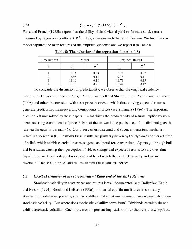
29
(18) .kkt%k ' ζk % χk ( Dt / q s
t&1 ) % ht ,k
Fama and French (1988b) report that the ability of the dividend yield to forecast stock returns,
measured by regression coefficient of (18), increases with the return horizon. We find that ourR 2
model captures the main features of the empirical evidence and we report it in Table 8.
Table 8: The behavior of the regression slopes in (18)
Time horizon Model Empirical Record
k χk R 2 χk R 2
1 2 3 4
5.03 8.66 11.16 13.10
0.08 0.14 0.18 0.21
5.32 9.08 11.73 13.44
0.07 0.11 0.15 0.17
To conclude the discussion of predictability, we observe that the empirical evidence
reported by Fama and French (1998a, 1998b), Campbell and Shiller (1988), Poterba and Summers
(1998) and others is consistent with asset price theories in which time-varying expected returns
generate predictable, mean-reverting components of prices (see Summers (1986)). The important
question left unresolved by these papers is what drives the predictability of returns implied by such
mean-reverting components of prices? Part of the answer is the persistence of the dividend growth
rate via the equilibrium map (6). Our theory offers a second and stronger persistent mechanism
which is also seen in (6). It shows these results are primarily driven by the dynamics of market state
of beliefs which exhibit correlation across agents and persistence over time. Agents go through bull
and bear states causing their perception of risk to change and expected returns to vary over time.
Equilibrium asset prices depend upon states of belief which then exhibit memory and mean
reversion. Hence both prices and returns exhibit these same properties.
6.2 GARCH Behavior of the Price-dividend Ratio and of the Risky Returns
Stochastic volatility in asset prices and returns is well documented (e.g. Bollerslev, Engle
and Nelson (1994), Brock and LeBaron (1996)). In partial equilibrium finance it is virtually
standard to model asset prices by stochastic differential equations, assuming an exogenously driven
stochastic volatility. But where does stochastic volatility come from? Dividends certainly do not
exhibit stochastic volatility. One of the most important implication of our theory is that it explains

30
why asset prices and returns exhibit stochastic volatility. We start by presenting in Figures 5 and 6
the results of simulated 500 observations: in Figure 5 we report price/dividend ratios and in Figure
6 the associated risky rates of return. These figures reveal time varying volatility reflected in time
variability of the variance of prices and returns. However, GARCH behavior is more subtle than
just volatility clustering; it requires volatility to be persistent and this requires a formal test.
FIGURE 5 PLACE HERE
FIGURE 6 PLACE HERE
To formally test the GARCH property of the price/dividend ratio and of the risky returns we
used the 20,000 simulated observations discussed in the previous section. Using these data we
estimated the following econometric model of the dynamics of the log of the price/dividend ratio
log(q st ) ' κq
% µq log(q st&1) % ς
qt
(19) ςqt - N(0 , h q
t )
.h qt ' ξ
q0 % ξ
q1 (ςq
t&1 )2% ν
q1 h q
t&1
Since the price dividend ratio is postulated to be an AR(1) process, the process in (19) is
GARCH(1,1). Similarly, for the risky rates of return we postulated the econometric model
kst ' κk % µk log(q s
t ) % ςkt
(20) ςk
t - N(0 , h k
t )
.h k
t ' ξk
0 % ξk
1 ( ςkt&1)2% ν
k
1 h k
t&1
For a specification of (19) and (20) we have also tested ARCH(1) and GARCH(2,1) but have
concluded that the proposed GARCH(1,1) as in (19)-(20) , describes best the behavior of the data
over time. Due to the large sample we ignore standard error and report our model implies that the
estimated model for the log of the price-dividend ratio satisfies the GARCH(1,1) specification
log(q st ) ' 0.99001 % 0.69384 log(q s
t&1) % ςqt
ςqt - N(0 , h q
t )
.h qt ' 0.00592 % 0.02370( ςq
t&1 )2% 0.73920h q
t&1 , R 2' 0.481
For the risky rates of return the estimated model satisfies the GARCH(1,1) specification
kt ' 1.13561 & 0.33355log(q st ) % ς
k
t
ςk
t - N(0 , h k
t )
.h k
t ' 0.00505 % 0.01714(ςkt&1)2% 0.77596h k
t&1 , R 2' 0.180

31
Stochastic volatility in our model is a direct consequence of the dynamics of the market
beliefs . It is clear that persistence of beliefs and correlation across agents introducezt ' (z 1t , z 2
t )
similar patterns into prices and returns. When agents disagree they offset the( i.e. z 1t z 2
t <0 )
demands of each other and as that pattern persists, prices do not need to change by very much for
markets to clear. During such periods prices exhibit low volatility hence persistence of belief states
induce persistence of low volatility. When agents agree they compete for the same(i.e. z 1t z 2
t > 0)
assets and prices are determined by difference in belief levels. Changes in the levels of bull or bear
states (i.e. values of ) generate high volatility in asset prices and returns. Persistence of(g 1t , g 2
t )
beliefs cause such high volatility regimes to exhibit persistence. Market volatility is then time
dependent. It changes with the market state of beliefs and hence it has a predictable component as
in (19)-(20). These results extend the earlier and similar result in Kurz and Motolese (2001).
The virtue of the above argument is that it explains stochastic volatility as an endogenous
consequence of equilibrium dynamics. Some “fundamental” shocks (i.e. an oil shock) surely cause
market volatility, but it has been empirically established that market volatility cannot be explained
consistently by repeated “fundamental” exogenous shocks (see Pesaran and Timmermann (1995)).
Our explanation of stochastic volatility is thus consistent with the empirical evidence
7. Concluding Remarks
This paper presents a unified paradigm which proposes that market volatility is driven
primarily by market expectations. This conclusion extends our previous work (cited earlier) on the
subject. The central new development is the formal introduction of the state of belief as a key tool
of General Equilibrium analysis and a corresponding requirement for agents to forecast the market
state of belief. Agents forecasting the state of belief of “others” is a precise mathematical structure
which embodies the Keynesian intuitive “Beauty Contest” aspect of asset pricing. On a deeper level
diverse individual forecasts of future market states of belief is equivalent to heterogenous forecasts
of future asset prices. Hence diverse price forecasting is the essence of our theory. In a general
equilibrium context the tool of a market state of belief is a formal method for allowing agents to be
rational yet make heterogenous price forecasts. Given the general structure of equilibria with
diverse and time dependent beliefs, we introduced the RB rationality principle and explored the

32
restrictions it imposes on the beliefs of the agents in the economy.
We have then constructed a simple model and tested it on all aspects of market volatility and
found the model to match well the empirical record. The structure of the model is applicable to any
phenomenon associated with market volatility since our main results are qualitative rather than
quantitative. The volatility results are driven by two crucial characteristics of the distribution of
market beliefs. These are (i) over confidence of an agent’ forecasts described by amplification of
the agent’s probabilities which, in turn, generate densities with fat tails, and (ii) asymmetry in the
frequency of bull or bear states.
References
Abel, A.B.: Asset Prices Under Habit Formation and Catching Up With the Joneses. AmericanEconomic Review (Papers and Proceedings) 80, 38 - 42 (1990).
Abel, A.B.: Risk Premia and Term Premia in General Equilibrium. Journal of MonetaryEconomics 43, 3 - 33 (1999)
Allen, F., Morris, S., Shin, H.S.: Beauty Contests and Iterated Expectations in Asset Markets. Working paper, (2003)
Backus, D. K., Gregory, A.W., Zin, S.E.: Risk Premiums in the Term Structure: Evidence fromArtificial Economies. Journal of Monetary Economics 24, 371 - 399 (1989).
Barberis, N., Huang, M., Santos, T.: Prospect Theory and Asset Prices. Quarterly Journal ofEconomics CXVI, 1-53 (2001).
Bollerslev, T., Engle, R., Nelson, D.: ARCH Models. In Engle, R., McFadden, G., (eds.)Handbook Of Econometrics, Vol. IV, Amsterdam: North Holland (1994).
Breeden, D.T.: An Intertemporal Asset Pricing Model with Stochastic Consumption andInvestment Opportunities. Journal of Financial Economics, 7, 265 - 296 (1979).
Brennan, M.J., Xia, Y.: Stock Price Volatility, Learning, and the Equity Premium. UCLA,Anderson School, February (1998).
Brock, W.A., LeBaron, B.D.: A Dynamic Structural Model for Stock Return Volatility andTrading Volume. The Review of Economics and Statistics 78 , 94 -110 (1996).
Campbell, J. Y.: Asset Prices, Consumption and the Business Cycle. Taylor, J. B., Woodford, M.(ed.) Handbook of Macroeconomics, Volume 1C, Chapter 19, 1231-1303 (2000).
Campbell, J.Y., Cochrane, J.H.: By Force of Habit: A Consumption-Based Explanation ofAggregate Stock Market Behavior. Journal of Political Economy, 107, 205 - 251 (1999).
Campbell, J. Y., Cochrane, J. H.: Explaining the Poor Performance of Consumption-Based AssetPricing Models. The Journal of Finance, 55, 2863-2878 (2000).
Campbell, J.Y., Shiller, R.J.: Stock Prices, Earnings, and Expected Dividends. Journal of Finance 43, 661-676 (1988).
Campbell, J. Y., Shiller, R. J. : Yield Spreads and Interest Rate Movements: A Bird’s Eye View.Review of Economic Studies, 58, 495 - 514 (1991).

33
Camerer, C., Lovallo, D.,: Overconfidence and Excess Entry: An Experimental Approach.American Economic Review, 89, 306 - 318 (1999).
Cecchetti, S., Lam, P., Mark, N.: Mean Reversion in Equilibrium Asset Prices. AmericanEconomic Review 80, 398 - 418 (1990).
Cecchetti, S., Lam, P., Mark, N.: The Equity Premium and the Risk-Free Rate: Matching theMoments. Journal of Monetary Economics, 31, 21 - 45 (1993).
Constantinides, G. : Habit Formation: A Resolution of the Equity Premium Puzzle. Journal ofPolitical Economy 98, 519 - 543 (1990).
Engel, C. M.: “The Forward Discount Anomaly and the Risk Premium: Survey of RecentEvidence.” Journal of Empirical Finance, 3, 123 - 192 (1996).
Epstein, L.G., Zin, S.E.: First-Order" Risk Aversion and the Equity Premium Puzzle. Journal ofMonetary Economics 26, 387 - 407 (1990).
Fama, E.F., French, K.R.: Permanent and Temporary Components of Stock Prices.Journal of Political Economy 96, 246-273 (1988a).
Fama, E.F., French, K.R.: Dividend Yields and Expected Stock Returns. Journal of FinancialEconomics 22, 3-25 (1988b).
Fan, M.: Evolving Term Structure with Heterogenous Beliefs. Manuscript, Department ofEconomics, Stanford University, August (2003).
Froot, K.A., Frankel, J.A.: Forward Discount Bias: Is it an Exchange Risk Premium? QuarterlyJournal of Economics 104, 139-161 (1989) .
Grossman, S.J., Shiller, R. J.: The Determinants of the Variability of Stock Market Prices. American Economic Review (Papers and Proceedings) 71, 222 - 227 (1981).
Heaton, J., Lucas, D.J.: Evaluating the Effects of Incomplete Markets on Risk Sharing and AssetPricing. Journal of Political Economy 104, 443-487 (1996).
Hansen, L.P., Singleton, K.L.: Stochastic Consumption, Risk Aversion, and the TemporalBehavior of Asset Returns. Journal of Political Economy, 91, 249 - 268 (1983).
Jin, H., Judd, K.: Perturbation Method for General Dynamic Stochastic Models. StanfordUniversity, http://www.stanford.edu/group/site/judd.03.2.pdf (2002)
Jin, H.: PSD - A Perturbation Solver for Dynamic Systems. Stanford University, Department ofEconomics, http://www.stanford.edu/~jinhehui/psdman.pdf (2003)
Kocherlakota, N.R.: The Equity Premium: It’s Still a Puzzle. Journal of Economic Literature, 34,42 -71 (1996).
Kurz, M.: On the Structure and Diversity of Rational Beliefs. Economic Theory 4, pp. 877 - 900 (1994). (An edited version appears as Chapter 2 of Kurz, M. (ed.).: 1997)
Kurz, M. (ed.): Symposium: Rational Beliefs and Endogenous Uncertainty. Economic Theory, 8,383 - 553 (1996).
Kurz, M. (ed): Endogenous Economic Fluctuations: Studies in the Theory of Rational Belief. Studies in Economic Theory, No. 6, Berlin and New York: Springer-Verlag (1997).
Kurz, M., Beltratti, A.: The Equity Premium is no Puzzle. Chapter 11 in Kurz, M. (ed.)Endogenous Economic Fluctuations: Studies in the Theory of Rational Belief. Studies inEconomic Theory, No. 6, Berlin and New York: Springer-Verlag, 283 -316 (1997).
Kurz, M., Jin, H., Motolese, M.: Endogenous Fluctuations and the Role of Monetary Policy.Chapter 10 in Aghion, P., Frydman, R., Stiglitz, J., Woodford, M. (ed.) Knowledge,

34
Information, and Expectations in Modern Macroeconomics, in Honor of Edmund S.Phelps, Princeton: Princeton University Press, 188 - 227 (2003a).
Kurz, M., Jin, H., Motolese, M.: The Role of Expectations in Economic Fluctuations and theEfficacy of Monetary Policy. Working Paper No. 03-010, Department of Economics,Stanford University, November 12, (2003b), to appear in Journal of Economics Dynamicsand Control (2005).
Kurz, M., Schneider, M.: Coordination and Correlation in Markov Rational Belief Equilibria.Economic Theory 8, pp. 489 - 520 (1996).
Kurz, M., Motolese, M.: Endogenous Uncertainty and Market Volatility. Economic Theory, 17,497 - 544 (2001).
Kurz, M., Wu, H.M.: Endogenous Uncertainty in a General Equilibrium Model. Economic Theory 8, pp. 461 - 488 (1996).
LeRoy, S. F.: Risk Aversion and the Martingale Property of Stock Prices. International EconomicReview, 14, 436 - 446 (1973).
Lucas, R. E. Jr.: Asset Prices in an Exchange Economy. Econometrica, 46, 1429 -1445 (1978).Mankiw, G. N.: The Equity Premium and the Concentration of Aggregate Shocks. Journal of
Monetary Economics, 15, 145 - 161 (1986).Mehra, R., Prescott, E. C. : The Equity Premium: A Puzzle. Journal of Monetary Economics 15,
145-162 (1985).Morris, S., Shin, H.S.: Social Value of Public Information. American Economic Review, 92 1521 -
1534 (2002).Nielsen, K. C. : Rational Belief Structures and Rational Belief Equilibria. Economic Theory, 8,
339 - 422 (1996).Nielsen, K. C. : Floating Exchange Rates vs. A Monetary Union Under Rational Beliefs: The Role
of Endogenous Uncertainty. Economic Theory, 21, 347 - 398 (2003).Paye, B., Timmermann, A.: Instability of Return Prediction Models. Mimeo, UCSD (2003).Pesaran, H., Timmermann, A.: Predictability of Stock Returns: Robustness and Economic
Significance. Journal of Finance, 50, 1201-1228 (1995).Poterba, J.M., Summers, L.H.: Mean Reversion in Stock Prices: Evidence and Implications.
Journal of Financial Economics 22, 27-29 (1988).Radner, R. : Existence of equilibrium of plans, prices and price expectations in a sequence of
Markets. Econometrica 40, 289-303 (1972).Reitz, T.A.: The Equity Premium: A Solution. Journal of Monetary Economics 22, 117 - 133
(1988).Rodriguez, J.C.: Consumption, the Persistence of Shocks, and Asset Pricing Puzzles. Draft,
Department of Economics, University of Maryland (2002).Summers, L.H.: Does the Stock Market Rationally Reflect Fundamental Values? Journal of
Finance 41, 591-601 (1986).Shiller, R. J.: Do Stock Prices Move Too Much to Be Justified by Subsequent Changes in
Dividends. American Economic Review 71, 421 - 435 (1981).Shilling, G. A.: Market Timing: Better Than Buy-and-Hold Strategy. Financial Analysis Journal,
48, 46 - 50 (1992).Svenson, O.: Are We All Less Risky and More Skillful Than Our Fellow Drivers? Acta

35
Psychologica, 47, 143 - 148 (1981).Timmermann, A.: Excess Volatility and Predictability of Stock Prices in Autoregressive Dividend
Model with Learning. Review of Economic Studies, 63, 523 - 557 (1996).Weil, P.: The Equity Premium Puzzle and the Riskfree Rate Puzzle. Journal of Monetary
Economics, 24, 401 - 422 (1989).Woodford, M.: Imperfect Common Knowledge and the Effect of Monetary Policy. Chapter 1 in
Aghion, P., Frydman, R., Stiglitz, J., Woodford, M. (ed.) Knowledge, Information andExpectations in Modern Macroeconomics, in Honor of Edmund S. Phelps Princeton:Princeton University Press, 25 -58 (2003).
Wu, H. W., W.C. Guo: Speculative Trading with Rational Belief and Endogenous Uncertainty.Economic Theory 21, 263 - 292 (2003).
Wu, H. W., W.C. Guo: Asset Price Volatility and Trading Volume with Rational Beliefs.Economic Theory 23, 795 -830 (2004).
APPENDIXESAppendix A: construction of the random variables ηj
t%1(uj
t )
In the text we defined . Since computations use standard normalφ(u jt ) ' 1/ (1%e
b(u jt &a)
)
variables we normalize u as follows
(A1) where , and . φ(u jt ) ' 1
1%eb(u j
t &a)' φ(u j
t) '1
1%eb(u j
t&a)b ' bσu j
ta'a/σu j
tu j
t-N(0,1)
A.1 The density function
The variables are now defined by specifying their density, conditional on :ηjt%1(u
jt) u j
t
p(ηjt%1*u
jt) '
φ1(ujt) f(ηj
t%1) if ηjt%1 $ 0
φ2(ujt) f(ηj
t%1) if ηjt%1 < 0
where is the standard normal density function and f(ηjt%1) '
1
2πe&
(ηjt%1)2
2
φ1(ujt) '
φ(u jt)
G, φ2(u
jt) ' 2&φ1(u
jt), G ' m
4
&4
φ(u jt)
1
2πe
(u jt)
2
2 du jt
Note that , which ensures that the rationality conditions be satisfied, i.e.Eφ1(ujt) ' Eφ2(u
jt)'1
(A2) m4
&4
p(ηjt%1|u
jt)Φ(u j
t)du jt 'Φ(ηj
t%1).
We need another condition to make sure that is a density function for all . This requiresp(ηjt%1|u
jt) u j
t
for all , which implies .φ2(ujt) $ 0 u j
t G $ 1/2

36
A.2 The moments of ηjt%1(u
jt )
A direct computations of the moments of this random variable leads to
(A3) E[ηjt%1|u
jt] '
φ1(ujt)
2π m4
0xe
&
x 2
2 dx %φ2(u
jt)
2π m0
&4
xe&
x 2
2 dx 'φ(u j
t)
G&1
2
2π
(A4) E[(ηjt%1)
2|u jt] '
φ1(ujt)
2π m4
0x 2e
&
x 2
2 dx %φ2(u
jt)
2π m0
&4
x 2e&
x 2
2 dx ' φ1(ujt)0.5 % φ2(u
jt)0.5 ' 1
Since and we have and Eφ1'Eφ2'1 Eu jt'0 E[ηj
t%1]'0, E[(ηjt%1 )2]'1 E[ηj
t%1ujt] '
2
2π
E[φ(u jt)u
jt]
G.
Note that, given (A1) and the parameter choice b < 0, defined in (A3) is aE[ηjt%1|u
jt]
monotone increasing function in . It is straightforward to show that for any u jt φ(u j
t) > G u jt > a
and for any hence if and if .φ(u jt) < G u j
t < a E[ηjt%1|u
jt] > 0 u j
t > a E[ηjt%1|u
jt] < 0 u j
t < a
We now reformulate the random variable as used in the computational model. Letηjt%1(u
jt )
and define µ(u jt) / E[ηj
t%1|ujt] , s(u j
t) / E[(ηjt%1)
2|u jt]&(E[ηj
t%1|ujt])
2 , νjt%1 /
ηjt%1&µ(u j
t)
s(u jt)
(A5) . ηjt%1(u
jt) ' µ(u j
t)%s(u jt)ν
jt%1
Appendix B: Statement of the Rationality Conditions
The rationality of belief principle requires that
(B1) has the same joint empirical distribution as .Ψt%1(uj
t ) '
λxg η
jt%1 (u j
t ) % ρx j
t%1
λzgη
jt%1 (u j
t ) % ρz j1
t%1
λzgη
jt%1 (u j
t ) % ρz j2
t%1
ρt%1 '
ρxt%1
ρz 1
t%1
ρz 2
t%1
when is considered part of the variability of the term on the left.u jt , t ' 1 ,2 , ....
To understand (B1) keep in mind the consistency conditions for all t. These areg jt ' z j
t
macroeconomic consistency condition (like market clearing conditions) but they do not hold in the
agent’s perception model who treats the as exogenous variables. In the agent’s perceptionz jt
model there is nothing to require the covariance between gj and any state variable to be the same as
the covariance implied by (7a)-(7c) between zj and that variable. The presence of in allηjt%1(u
jt )
equations of (11a)-(11c) generates perceived covariance between gj and observed state variables

37
that may not be in (7a)-(7c). Any covariance between an agent’s own gj and other variables in the
economy are strictly in the mind of the agent and no rationality conditions are imposed on them.
We show first that (B1) fully pins down the covariance matrix of the three dimensionalΩjρρ
vector in (11a)-(11d). We write all j because of symmetry. To directlyρjt%1 Ω
jρρ'Ω
ρρ
demonstrate why is pinned down by (B1), use it to rewrite (9a) in the formΩρρ
(B2) , and (a , b) given.w jt%1 ' Awt % λgη
jt%1(u j
t ) % ρjt%1 , λg ' (λx
g , λzg , λz
g)N
Now define and recall that V is the covariance matrix of according toσ2η' E[(ηj
t%1( u jt ) )2] wt
the empirical distribution defined in (9). Computing the covariance matrix in (B2) and equating the
computed value to V leads to the equality which means thatV ' AVAN % λg(λg)Nσ2η% Ω
ρρ
(B3) .Ωρρ' V & AVAN & λg(λg)Nσ
2η
For any (a, b, ), magnitudes on the right of (B3) are known and this pins down the matrix λg Ωρρ
The perception model of an agent includes the transition equation for in (5) and thisg jt%1
implies that the agent’s model specifies a full joint distribution of four variables: three observables
wt and . Hence, we specify a 4×4 covariance matrix Ω of the innovations which is written as. g jt
Ω '
Ωρρ
, Ωwg
ΩN
wg , σ2g
where = is a 3×1 covariance vector. InΩwg [Cov( ρxt%1 , ρg j
t%1 ) , Cov( ρz 1
t%1 , ρg j
t%1 ) , Cov( ρz 2
t%1 , ρg j
t%1 )]
addition we now define the following
- unconditional covariance vector between gj and the four observables w;r j/ Cov(w , g j )
- vector of w parameters in the gj equation (5).a j' (λz j
x , 0 , 0)
By symmetry, both terms are the same for all j. To compute r we multiply (5) by the first three
equations in (11a)-(11c) and compute the three equations to define the unconditional covariance as
r ' λzAr % AVa % λzλgrηuσu % Ωwg
hence the 3×1 covariance vector of the innovations of the agent’s belief must satisfy
(B4) .Ωwg ' r & λzAr & AVa % λzλgrηuσu
. By (B4) is pinned down when we specify . rηu ' E[
ηt%1(u)g
σu
] ' E[ηt%1(u)u
σu
] Ωwg r / Cov(w , g j)
A simpler approach is to treat (B4) as a system of 3 equations in the 6 unknowns (r, ). For nowΩxg
we have only 3 restrictions in (B4). We now show that our theory provides three additional

38
restrictions to determined (r, ). To explore the added implied restrictions we first utilize theΩxg
definition of anonymity:
Covariance Implications of Anonymity: Anonymity requires the idiosyncratic component of an
agent’s belief not to be correlated with market beliefs. It implies that in a symmetric equilibrium the
unconditional correlation between an agent’s state of belief and the belief of “others’ is the same
across agents. We translate this to require that
(B5a) Ωz 1g j ' Cov( ρz 1
t%1 , ρg j
t%1 ) ' 0
(B5b) .Ωz 2g j ' Cov( ρz 2
t%1 , ρg j
t%1) ' 0
(B5a)-(B5b) restricts the vector r to satisfy . (Ωwg)2 ' (Ωwg)3 ' 0
We need one more restriction and we show that it is deduced from the rationality condition
requiring to be serially uncorrelated. We claim that for to exhibit no serialΨt%1(u jt ) Ψt%1(u j
t )
correlation it is sufficient that it is uncorrelated with date t public information. To see why, recall
and suppose is uncorrelated with observables up to date t. Hence Ψt%1(uj
t ) ' wt%1&Awt Ψt%1(u jt )
.E[Ψt%1(u jt ) Ψt( u j
t&1 )] ' E[Ψt%1( u jt )(wt & Awt&1)] ' E[Ψt%1( u j
t ) wt] & E[Ψt%1( u jt )Awt&1] ' 0
To ensure these conclusions hold we put restrictions on r which imply that are uncorrelatedu jt
with any Recall first that by the definition of the filter we havewt&i , for all i $ 0. u jt
.u jt / u( g j
t ) ' g jt & r NV &1wt
The requirement is a simple implication of the filter since . ToCov(u jt , wt) ' 0 r j
t / Cov( wt , g jt )
examine the requirement , recall that the agent’s model (11a)-(11d) specifiesCov(u jt%1 , wt) ' 0
.w jt%1 ' Awt % λgη
jt%1 (ut ) % ρ
jt%1
Hence we have
.u jt%1 / u(g j
t%1 ) ' g jt%1& r NV &1w j
t%1 ' λzgj
t %aNwt% ρg j
t%1& rNV &1(Awt%λgηjt%1 (ut )% ρ
jt%1 )
Consequently, the condition would be satisfied if Cov(u jt%1 , wt) / E[ u j
t%1 wtN] ' 0
(B6) . λz rN % aNV & rNV &1 AV ' 0
Although (B6) is a system of 3 equations, we now show that (B6) is actually the last restriction
implied by the rationality of belief conditions. To see this fact note that since V is an invertible
matrix, the equations (B6) can be solved for the covariance vector , implyingr
(B7) .[AN & λz I] V &1 rN ' a
We study only the case . In this case the matrix takes the following formλz 1 ' λz 2 ' λz AN

39
AN '
λx , λzx , λ
zx
0 , λz , 00 , 0 , λz
hence is singular with the last two rows being zero. This is compatible with the fact[AN & λz I]
that hence, the system (B7) consists of only one restriction. a ' (λzx , 0 , 0 )
We can conclude that (B4) together with the conditions and (B7)(Ωwg)2 ' (Ωwg)3 ' 0
completely determine (r, ). Finally, when r is known, is pinned down as follows. Since weΩwg σ2
g j
know that , we use the condition to compute σ2
u j ' var( g j ) & rNV &1r var(g j ) ' var( z j )
.σ2
g j ' ( 1 & λ2z ) var(g j ) & aNVa & 2λzaNr
Appendix C: the computational model
This appendix explores several computational issues which have not been discussed in the text. We
want to provide here a complete description of the computed equilibrium conditions.
C.1 Equilibrium set and indeterminacy in the riskless economy
To ensure the existence of bounded solutions and hence exclude explosive solutions which
violate transversality we impose quadratic utility penalties on deviation of asset holdings away from
steady state. The penalty functions are: for stock holdings and forD 1&γt
τs
2(θj
t&0.5)2 D &1&γt
τB
2(B j
t )2
bond holdings with . The penalty functions are then subtracted from utility.τs ' τB ' 0.005
Indeterminacy of the optimal portfolio allocation at the riskless steady state is also a
problem for perturbation models with a number of financial assets greater or equal to two. This is
due to the fact that financial assets exhibit the same rate of return in the riskless economy hence are
perfect substitutes. Penalty functions ensure the steady state solution and is unique.θjt ' 0.5 B j
t ' 0
C.2 The revised optimization problem and the system of Euler equations
Given the above, the optimization problem of agent j is then reformulated as follows:
Max(C j,θj ,B j)
EQ j j4
t'0
βt 11&γ
(C jt ) 1&γ
&D 1&γt
τs
2(θj
t&0.5) 2&D &1&γ
t
τB
2(B j
t ) 2 | Ht , g jt
subject to:

40
C jt % qs
t θjt % q b
t B jt ' Λ
jt % ( qs
t % Dt )θjt&1 % B j
t&1
The Euler equations are:
(C jt )&γq s
t % D 1&γt τs(θ
jt&0.5) ' βEQ j
t[ (C j
t%1 )&γ(q st%1 % Dt%1) | Ht , g j
t ]
(C jt )&γq b
t % D &γ&1t τB(B j
t ) ' βEQ jt[(C j
t%1 )&γ | Ht , g jt ]
After normalization the budget constraint becomes:
c jt % q s
t θjt % q b
t b jt ' ω % (q s
t % 1)θjt&1 % b j
t&1 e&xt
and the Euler equations become:
(c jt )&γq s
t % τs(θjt&0.5) ' βEQ j
t[ ( c j
t%1 )&γ (1 % q st%1 )e
(1 & γ )xt%1 | Ht , g jt ]
(c jt )&γq b
t % τb(bj
t ) ' βEQ jt[ ( c j
t%1 )&γ e&γxt%1 | Ht , g j
t ]
C.3 The riskless steady state
In the riskless steady state quantities are as follows:
b 1('b 2(
' 0, θ1('θ2(
' 0.5, c 1('c 2(
' ω%0.5.
And prices are:
q s'
βe x ((1&γ)
1&βe x ((1&γ), q b
' βe &γx (
.
C.4 The perturbation structure
We specify here how we formulated the perturbation model. Let g be the perturbation
variable then the perturbation structure of the agent's perception model is as follows:
x jt%1 ' (1 & λx)x (
% λx xt % λxy η
jt%1( u j
t , ε ) % ερx j
t%1
z j1t%1 ' λzz 1
t % λzx (xt & x () % λ
zy η
jt%1( u j
t , g ) % gρz j1
t%1
z j2t%1 ' λzz 2
t % λzx (xt & x () % λ
zy η
jt%1( u j
t , g ) % gρz j2
t%1
g jt%1 ' λz g j
t % λzx ( xt & x () % g ρ
g j
t%1
where as defined in (A3)-(A5) of Appendix A.ηjt%1( u j
t , g ) ' µ(u jt) % g s( u j
t )νjt%1

Figure 1: Non-Normal Belief Densities.
6
-
gj > 0 gj < 0
ηj(gj)
-
6
ηj(gj)
Empirical Distribution
®
Empirical Distribution
U
Figure 2: Density of Ψ(gjt ) with Fat Tails.
6
-
Empirical Distribution
gj < 0gj > 0Bear Bull
° °N
λxgηj
t+1
(gj
t
)+ ρxj
t+1

Figure 3: Variance Ratios.
0.2
0.4
0.6
0.8
0 5 10 15 20
Figure 4: Properties of Returns from regression (17).
-0.4
-0.2
0
0.2
0 5 10 15 20 25 30 35 40
the slope δk
R2

Figure 5: Log of Price-dividend ratios.
2.6
2.8
3
3.2
3.4
3.6
Figure 6: Log of Risky Rates of Return.
-0.4
-0.2
0
0.2
0.4
0.6