This article was downloaded by: [Universite Laval]On: 13 July 2014, At: 19:40Publisher: RoutledgeInforma Ltd Registered in England and Wales Registered Number: 1072954 Registered office: Mortimer House,37-41 Mortimer Street, London W1T 3JH, UK

Click for updates

Applied EconomicsPublication details, including instructions for authors and subscription information:http://www.tandfonline.com/loi/raec20

Determinants of renewable energy adoption in Chinaand India: a comparative analysisShuddhasattwa Rafiqa, Harry Blochb & Ruhul Salimb

a Graduate School of Business, Deakin University, Melbourne, Australiab School of Economics & Finance, Curtin University, Perth 6845, AustraliaPublished online: 23 Apr 2014.

To cite this article: Shuddhasattwa Rafiq, Harry Bloch & Ruhul Salim (2014) Determinants of renewable energy adoption inChina and India: a comparative analysis, Applied Economics, 46:22, 2700-2710, DOI: 10.1080/00036846.2014.909577

To link to this article: http://dx.doi.org/10.1080/00036846.2014.909577

PLEASE SCROLL DOWN FOR ARTICLE

Taylor & Francis makes every effort to ensure the accuracy of all the information (the “Content”) containedin the publications on our platform. However, Taylor & Francis, our agents, and our licensors make norepresentations or warranties whatsoever as to the accuracy, completeness, or suitability for any purpose of theContent. Any opinions and views expressed in this publication are the opinions and views of the authors, andare not the views of or endorsed by Taylor & Francis. The accuracy of the Content should not be relied upon andshould be independently verified with primary sources of information. Taylor and Francis shall not be liable forany losses, actions, claims, proceedings, demands, costs, expenses, damages, and other liabilities whatsoeveror howsoever caused arising directly or indirectly in connection with, in relation to or arising out of the use ofthe Content.

This article may be used for research, teaching, and private study purposes. Any substantial or systematicreproduction, redistribution, reselling, loan, sub-licensing, systematic supply, or distribution in anyform to anyone is expressly forbidden. Terms & Conditions of access and use can be found at http://www.tandfonline.com/page/terms-and-conditions

Determinants of renewable energy

adoption in China and India: a

comparative analysis

Shuddhasattwa Rafiqa, Harry Blochb and Ruhul Salimb,*aGraduate School of Business, Deakin University, Melbourne, AustraliabSchool of Economics & Finance, Curtin University, Perth 6845, Australia

This article examines the dynamic relationships among output, carbon emis-sion and renewable energy generation of India and China during the period1972 to 2011 using a multivariate vector error correction model (VECM). Theresults for India reveal unidirectional short-run causality from carbon emissionto renewable energy generation and from renewable energy generation tooutput, whereas in the long run, the variables have bidirectional causality.Causalities in China give a rather different scenario, with a short-run unidir-ectional causality from output to renewable energy and from carbon emissionto renewable energy generation. In the long run, for China, unidirectionalcausality is found from output to renewable energy generation, while bidirec-tional causality is found between carbon emission and renewable energygeneration.

Keywords: renewable energy; CO2 emission; time series data; vector errorcorrection model; causality

JEL Classification: C22; C32; Q20; Q43; Q48

I. Introduction

The increasing threat of climate change and globalwarming per se has called for more discussion regard-ing the linkage between economic growth and pollu-tant emission all over the world. Carbon dioxide (CO2)is considered to be the main greenhouse gas (GHG)leading to global warming (The World Bank, 2007).CO2 emissions have the nature of the ‘tragedy of thecommons’ and an emerging economy may not beinterested in reducing CO2 emissions during its rapideconomic expansion phase. Growing concerns overeconomic growth, climate change and energy depen-dence are nevertheless driving specific policies to sup-port renewable energy resources and more efficientenergy usage in some emerging economies, so that

economic growth can be sustained without exertingharmful impacts on the environment.

The rapid growth of the Chinese and Indian econo-mies has increased their energy demand, posing difficultquestions of the appropriate use of scarce nonrenewableenergy and the extent to which renewable energy may besubstituted. Recent renewable energy generation data ofthese two countries show an encouraging and increasingtrend. Hence, identifying linkages that are behind theadoption of cleaner energy at this stage of developmentis worth academic research.

China emitted approximately 23.99% of the world’stotal carbon dioxide (CO2) in 2009 (The World Bank,2011). This may be attributed to two reasons. The firstreason is China’s enormous use of fossil fuels, particularlycoal. Second, China’s consumption of nonfossil energy

*Corresponding author. E-mail: Ruhul.Salim@cbs.curtin.edu.au

Applied Economics, 2014Vol. 46, No. 22, 2700–2710, http://dx.doi.org/10.1080/00036846.2014.909577

2700 © 2014 Taylor & Francis

Dow

nloa

ded

by [

Uni

vers

ite L

aval

] at

19:

40 1

3 Ju

ly 2

014

(i.e. hydro and nuclear electricity) accounted for only8.6% of its total energy consumption. The hope for thefuture is that China’s energy consumption policy willfollow the philosophy of reducing the overall intensity ofcarbon emissions by increasing the proportion of renew-able energy consumption in the total primary energyconsumption.

India was responsible for only about 6.18% of world’scarbon emission in 2009 (The World Bank, 2011). Eventhough India’s economy is growing very rapidly, energy isstill scarce and the country is not emitting that much CO2

when compared to China. This may be attributed to thefact that continuous electrification is still out of reach formany Indian rural households, and of these households arestill reliant on traditional biomass and biogas-type energysources for their day-to-day living.

In-depth studies identifying the linkage among output,CO2 emission and renewable energy for major emergingeconomies like China and India are limited in the litera-ture. Furthermore, none of the previous studies attempts tocompare the drivers behind the increased renewableenergy generation in these two economies. Identifyingthese linkages might help policy-makers to accelerate theadoption of cleaner energy in developing economies. Wecompare the drivers of renewable energy adoption in twomost prominent emerging economies, China and India,with the aim of analysing causality within an error correc-tion model formulation. This includes identifying thedirection of both short- and long-run causalities as wellas examining within-sample Granger exogeneity andendogeneity of each variable. Furthermore, to check therobustness of the causality directions and magnitude, wepresent variance decompositions (VDs) and impulseresponse functions (IRFs) that provide informationabout the interaction among the variables beyond thesample period.

This article is organized as follows. Section II providesa basic overview of the pollutant emission and renewable

energy adoption scenario in China and India and a criticalreview of literature. Section III delineates the theoreticalsettings and empirical methodology employed in thisarticle. Empirical results are offered in Section IV.Sections V and VI present the findings from generalizedIRFs and VDs, respectively. Finally, the conclusions anddiscussion of policy implications are offered inSection VII.

II. Literature Review

With sustained economic growth for more than threedecades, China and India both have lifted millions ofpeople out of poverty. However, these higher economicgrowth trends have their costs, as well. One of the triplebottom lines, environmental sustainability, has been threa-tened in recent years. The trend of carbon emission forboth of these countries shows an increasing pattern overthe period 2003 to 2011, while renewable energy genera-tion in China is rapidly increasing and is also rising inIndia.

Global new investment in renewable power and fuelswas USD 244 billion in 2012, down by 12% from theprevious year’s record (Table 1). This decline in invest-ment – after several years of growth – resulted fromuncertainty about support policies in major developedeconomies, especially in Europe (down 36%) and theUnited States (down 35%). The year 2012 saw the mostextreme shift yet in the balance of investment activitybetween developed and developing economies. Outlaysin developing countries reached USD 112 billion, repre-senting 46% of the world total. This was up from 34% in2011, and continued an unbroken 8-year growth trend. Bycontrast, investment in developed economies fell by 29%to USD 132 billion, the lowest level since 2009. The shiftwas primarily driven by reductions in subsidies for solar

Table 1. Global renewable energy investment trend

2010 2011 2012

Investment in new renewable energy capacity (annual)a Billion USD 227 279 244Renewable power capacity (total, including hydro) GW 1250 1355 1470Hydropower capacity (total)b GW 935 960 990Bio-power generation GWh 313 335 350Solar PV capacity (total) GW 40 71 100Concentrating solar thermal power (total) GW 1.1 1.6 2.5Wind power capacity GW 198 238 283Solar hot water capacity (total)c GWth 195 223 255Ethanol production (annual) Billion litres 85.0 84.2 83.1Biodiesel production (annual) Billion litres 18.5 22.4 22.5

Notes: aInvestment data are from Bloomberg New Energy Finance. bHydropower data do not include pumped storage capacity. cSolar hotwater capacity data include glazed water collectors only.Source: REN 21.

Renewable energy adoption in China and India 2701

Dow

nloa

ded

by [

Uni

vers

ite L

aval

] at

19:

40 1

3 Ju

ly 2

014

and wind project development in Europe and the UnitedStates, increased investor interest in emerging marketswith rising power demand and attractive renewable energyresources, and falling technology costs of wind and solarphotovoltaic (PV). Europe and China accounted for 60%of global investment in 2012 (REN21, 2013).

At the national level, the top investors in renewableenergy included four developing countries (most of theBRICS countries) and six developed countries. China wasin the lead with USD 64.7 billion invested, followed by theUnited States (USD 34.2 billion), Germany (USD 19.8billion), Japan (USD 16.0 billion) and Italy (USD 14.1billion). The subsequent five were the United Kingdom(USD 8.8 billion), India (USD 6.4 billion), South Africa(USD 5.7 billion), Brazil (USD 5.3 billion) and France(USD 4.6 billion).1

China accounted for USD 66.6 billion (including R&D)of renewable energy new investment, up 22% from 2011levels, driven by strong growth in the solar power sector,including both utility-scale2 and small-scale projects(<1 MW). New renewable energy investment in Indiahas also been increasing till 2011 (USD 13 billion in2011). However, like some developed countries, theinvestment dropped down to USD 6.5 billion. The trendin investment for the last decade nevertheless has beenupward as a whole.

Both India and China aspire to increase renewableenergy use as both of them are working towards loweringgrowth in carbon emissions. Some of the major targets inthis regard are presented in Table 2.

A substantial and growing amount of literature hasstudied the nexus between energy consumption and eco-nomic growth (for example, Kraft and Kraft, 1978; Ghosh,2002; Zamani, 2007; Ma et al., 2008; Apergis and Payne,2009;Wolde-Rufael, 2009; Bloch et al. 2012; Apergis andTang, 2013; Salamaliki and Venetis, 2013). Research onthis issue has primarily evolved around two differentprocedures, the supply-side and the demand-sideapproaches. The supply-side approach analyses the con-tribution of energy consumption in economic activitieswithin the traditional production function framework(Stern, 2000; Ghali and El-Sakka, 2004; Oh and Lee,2004; Sari and Soytas, 2007). While the demand-sideapproach investigates the relationship among energy con-sumption, gross domestic product (GDP) and energyprices (often taking CPI as a proxy) in a tri-variate energydemand model (Masih and Rumi, 1997; Asafu-Adjaye,2000; Narayan and Singh, 2007).3

Although pollutant emission is a very important com-ponent of growth-energy dynamics, many of the earlierstudies don’t include emission in their models. Somestudies that include carbon emission in their analyticalframeworks are Ang (2007), Apergis and Payne (2009),Chandran and Tang (2013) and Liu (2005); Arouri et al.,(2012) extend the findings of Ang (2007) and Apergis andPayne (2009), by implementing recent bootstrap panelunit root tests and cointegration techniques to investigatethe relationship among carbon dioxide emissions, energyconsumption and real GDP for 12 Middle East and NorthAfrican Countries (MENA) over the period 1981 to 2005.

Table 2. Renewable energy targets in India and China

Country Sector/technology Target

India Renewable electricity 53 GW capacity by 2017Wind 5 GW by 2017Solar 10 GW by 2017; 20 GW grid-connected by 2022; 2000MWoff-grid by 2020; 20 million

solar lighting systems by 2022.Small-scale hydro 2.1 GW by 2017Bioenergy 2.7 GW by 2017Solar water heating 5.6 GWth (8 million m2) of new capacity to be added between 2012 and 2017.

China Renewable electricity 49 GW capacity by 2013Wind 100 GWon-grid by 2015; 200 GW by 2020Solar PV 10 GW in 2013; 20 GW by 2015CSP 1 GW by 2015Hydro 290 GW by 2015Bioenergy 13 GW by 2015Solar thermal 280 GWth (400 million m2) by 2015

Note: GW, gigawatt, equal to one billion watts; CSP, concentrating solar power; PV, photovoltaic.Source: REN21

1National investment totals do not include government and corporate R&D because such data are not available for all of these countries.2Utility-scale refers to wind farms, solar parks and other renewable power installations of 1 MVor more in size, and biofuel plants withcapacity of more than 1 million litres.3 In addition to the above studies, recent research, such as Ang (2008), include pollutant emissions in their analyses to investigate therelationship between energy consumption and economic activities. However, since Ang does not include prices in the models, this is not acomplete demand-side model.

2702 S. Rafiq et al.

Dow

nloa

ded

by [

Uni

vers

ite L

aval

] at

19:

40 1

3 Ju

ly 2

014

Results show that, in the long run, energy consumptionhas a positive and significant impact on CO2 emissions.More interestingly, it has been shown that real GDP exhi-bits a quadratic relationship with CO2 emissions for theregion as a whole.

Pao and Tsai (2010) also employ a panel cointegrationframework to examine linkages among pollutant emis-sions, energy consumption and output for BRIC (Brazil,Russia, India, and China) countries. In the long-run equi-librium, energy consumption has a positive and statisti-cally significant impact on emissions, while real outputexhibits the inverted U-shape pattern associated with theenvironmental Kuznets curve (EKC) hypothesis. In theshort term, changes in emissions are driven mostly bythe error correction term (ECT) and short-term energyconsumption shocks, as opposed to short-term outputshocks for each country.

Employing different model settings, Minihan and Wu(2012) study economic structure and strategies for GHGmitigation. Their framework suggests that there are differ-ent technical options in GHG mitigation due to the eco-nomic linkages among different polluting activities.Another study on GHG emissions, energy consumptionand economic growth by Hamit-Haggar (2012) investi-gates the long-run equilibrium relationship by means ofthe fully modified OLS (FMOLS) technique proposed byPedroni (2000), finding that energy consumption has apositive and statistically significant impact on GHG emis-sions. In contrast, a nonlinear relationship is foundbetween GHG emissions and economic growth, which isconsistent with the EKC.

One of the recent studies focusing on China and India isChandran and Tang (2013). This study investigates theshort-run and long-run linkages among CO2 emission,economic growth and coal consumption of China andIndia from 1965 to 2009. This study finds cointegratingrelationships between the variables for China. However,this study fails to find any long-run relationship in case ofIndia. Bi-directional causality, in the short and long run, isdetected between economic growth and coal consumptionas well as between coal consumption and CO2 emissionsin China. In addition, uni-directional causality is detectedfrom economic growth to CO2 emissions. For India, thisstudy finds that a short-run bi-directional causality existsbetween economic growth and CO2 emissions andbetween CO2 emission and coal consumption. It has alsobeen found that economic growth Granger causes coalconsumption in the short run in India.

The drivers behind different types of nonrenewableenergy consumption (i.e. oil, gas and coal) have beenwell studied, but relatively little is known about the driversbehind renewable energy consumption. Studies that iden-tify the drivers for renewable energy in G7 countries and22 emerging countries are Sadorsky (2009a) and (2009b),respectively. Both these studies employ the panel

cointegration technique and find that renewable energyconsumption is driven by both carbon emissions andGDP in G7 countries, while only GDP is a driver indeveloping countries. Fang (2011) takes the supply-sideapproach to investigate the impact of renewable energy ineconomic development. Using Chinese data spanningfrom 1978 to 2008, the impact of renewable energy con-sumption in economic welfare is found to be insignificant.However, none of these studies includes pollutant emis-sion in their models.

Although pollutant emission is directly related toenergy generation and renewable energy adoption shouldhave some positive impact on emission scenario, only afew studies on renewable energy include carbon emissionin their models. Salim and Rafiq (2012) employ an auto-regressive distribution lag (ARDL) model along with fullymodified least square and dynamic ordinary least squaremodels for six major emerging economies, Brazil, China,India, Indonesia, Philippines and Turkey, over the period1980 to 2006. They find that both income and pollutantemission play a significant role in renewable energy gen-eration in Brazil, China, India and Indonesia, whileincome alone is the main determinant in Philippines andTurkey.

In summary, from the above review, it is evident thatthe relationship among economic growth, carbon emis-sion and renewable energy generation is not uniformacross countries or estimation method. There are a fewstudies on renewable energy consumption in China andIndia that consider emission in analysing the dynamicsbetween renewable energy and output. We utilize recentdevelopments in time-series analysis to examine both thesupply and demand approaches for both these countriesby applying an error correction model on the most recentdata. This provides an opportunity to examine similaritiesand differences in both short- and long-run causalitiesamong economic growth, carbon emissions and renew-able energy output.

III. Theoretical Framework

Variables selected in this study are based on economictheory and data availability. Real GDP is included in themodel to measure income; CO2 emission is included for itsdetrimental impact on the environment; and renewableenergy generation is included to understand the linkagesbetween renewable energy and the other variables. As allthe concerned variables can be considered to be endogen-ous within a single system, we employ a VAR-type modelwith three different equations to identify the dynamicrelationships among the variables. The equation for eco-nomic growth takes the following form:

Renewable energy adoption in China and India 2703

Dow

nloa

ded

by [

Uni

vers

ite L

aval

] at

19:

40 1

3 Ju

ly 2

014

LYt ¼ μi1 þXp�1

j¼1

β1jLYt�j þXp�1

j¼1

γ1jLERt�j

þXp�1

j¼1

δ1jLCt�j þ ε1t

(1)

where t = 1972, 1973,……., 2011 denotes the time period,εt is a white noise, ‘well-behaved’ random disturbanceterm with positive definite covariance matrix Ω. LY, LERand LC refer to the logarithm for real GDP, renewableenergy generation and carbon emission, respectively.

As is apparent from previous studies, two of the majordeterminants of renewable energy consumption areincome and carbon emission, so this study investigatesthe following equation:

LERt ¼ μ2 þXp�1

j¼1

β2jLERt�j þXp�1

j¼1

γ2jLYt�j

þXp�1

j¼1

δ2jLCt�j þ ε2t

(2)

Carbon emission is also determined by the level of eco-nomic activities and by the acceleration of adoption ofrenewable energy technologies in country. Hence, thefollowing equation completes the three-equation VARmodel:

LCt ¼ μ3 þXp�1

j¼1

β3jLCt�j þXp�1

j¼1

γ3jLYt�j

þXp�1

j¼1

δ3jLERt�j þ ε3t:

(3)

This study considers annual data of India and China overthe period 1972 to 2011 from World DevelopmentIndicators (WDI). Real GDP data have the base year of2005. Carbon emission data are in kilo tonnes of CO2

emission and renewable energy generation is electricityproduction from renewable sources (kWh).

The empirical estimation carried out has three objec-tives. The first objective is to understand how the variablesare linked in the long run; the second is to find the dynamiccausal relationship among the variables; and the third is toinvestigate the robustness of the causality directions andmagnitude. To achieve these objectives, a reduced-formvector auto regression (VAR) model is constructed withthree variables – output, carbon emission and renewableenergy generation. The VAR approach serves the estima-tion purpose, since it avoids imposing structural assump-tions by treating all variables as endogenous. The reduced-form level VAR is presented as:

zt ¼ α0 þXp

j¼1Ajzt�j þ εt (4)

where zt = [LYt, LCt, LERt]. The series LYt, LCt andLERt can be either I(0) or I(1). αt is a vector of constantterms or α0 ¼ ½αY ;αC;αRE� and Aj is a matrix of VARparameters for lag j. The vector of error termsis ε0 ¼ ½εY ; εc; εRE�t � INð0;ΩÞ.

Before implementing the error correction model, it isimperative to ensure first that the underlying data are non-stationary at level and there exists at least one cointegratingrelationship among variables. Hence, we implement aug-mented Dicky–Fuller (ADF), Phillips Perron (PP) andKwiatkowski–Phillips–Schmidt–Shin (KPSS) tests for datastationarity. All of these tests indicate that each of the vari-ables for both of the countries follow an I(1) process.However, these standard tests may not be appropriate whenthe series contains structural breaks (SalimandBloch, 2009).Therefore, we also employ two structural break tests. Perron(1997) develops a procedure for detecting a single structuralbreak that has been widely used in the literature. For India,Perron’s test identifies breaks at 2002, 1998 and 1994 forLIY (logarithm of Indian GDP), LIER (logarithm of Indianrenewable energy) and LIC (logarithm of Indian carbonemission), respectively. For China, the break dates for LCY(logarithm of Chinese GDP), LCER (logarithm of Chineserenewable energy and LCC (logarithm of Chinese carbonemission) are 1990, 2001 and 1996, respectively.

More recently, Lee and Strazicich (2003) develop ver-sions of the LM unit root test to accommodate two structuralbreaks. The endogenous two-break unit root test allows fortwo shifts in the intercept and is described by Zt = [1, t, D1t,D2t], whereDjt = 1 for t > Tbj + 1, j = 1, 2, and 0 otherwise.Tbj denotes the date of the structural break. Note that the datagenerating process (DGP) includes breaks under the null(β = 1) and alternative (β < 1) hypotheses in a consistentmanner. In this model, depending on the value of β, we havethe following null and alternative hypotheses:

H0 : yt ¼ μ0 þ d1B1t þ d2B2t þ yt�1 þ v1t (5)

HA : yt ¼ μ0 þ γt þ d1D1t þ d2D2t þ v2t (6)

where v1t and v2t are stationary error terms; Bjt = 1 fort = Tbj + 1, j = 1, 2 and 0 otherwise. This model can beextended by including two changes in the intercept and theslope and is described by Zt = [1, t, D1t, D2t, DT1t, DT2t],whereDTjt = t - Tbj for t > Tbj + 1, j = 1, 2 and 0 otherwise.For this extended model, the hypotheses are:

H0 : yt ¼ μ0 þ d1B1t þ d2B2t þ d3D1t þ d4D2t

þ yt�1þ v1t(7)

HA : yt ¼ μ0 þ γt þ d1D1t þ d2D2t þ d3DT1tþ d4DT2t þ v2t

(8)

2704 S. Rafiq et al.

Dow

nloa

ded

by [

Uni

vers

ite L

aval

] at

19:

40 1

3 Ju

ly 2

014

where v1t and v2t are stationary error terms; Bjt = 1 fort = Tbj + 1, j = 1, 2 and 0 otherwise. We use the method ofLee and Strazicich (2003) to test the existence of a possi-ble structural break.

As Engle and Granger (1987) demonstrate, cointegratedvariables must have an error correction representationwith an ECT incorporated into the model. Therefore, avector error correction model (VECM) is formulated torecover the information lost in the differencing process,thereby allowing for long-run equilibrium as well as short-run dynamics. Assuming that there is only one cointegra-tion relationship, the VECM constructed for this study canbe expressed as:

ΔLYt ¼ μ1 þ α11ECTt�1 þXp�1

j¼1

β1jΔLYt�j

þXp�1

j¼1

γ1jΔLERt�j þXp�1

j¼1

δ1jΔLCt�jþε1t(9)

ΔLERt ¼ μ2 þ α21ECTt�1 þXp�1

j¼1

β2jΔLERt�j

þXp�1

j¼1

γ2jΔLYt�j þXp�1

j¼1

δ2jΔLCt�jþε2t

(10)

ΔLCt ¼ μ3 þ α31ECTt�1 þXp�1

j¼1

β3jΔLCt�j

þXp�1

j¼1

γ3jΔLYt�j þXp�1

j¼1

δ3jΔLERt�jþε3t

(11)

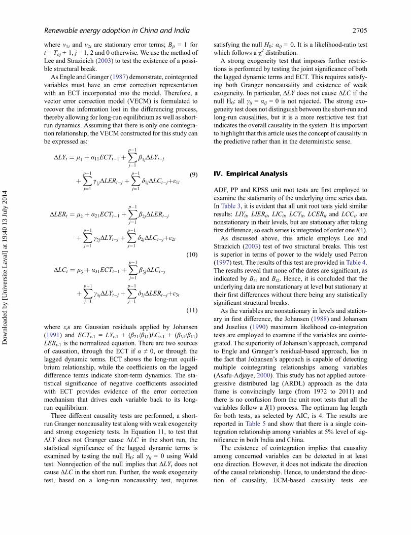
where εts are Gaussian residuals applied by Johansen(1991) and ECTt-1 = LYt-1 + (β21/β11)LCt-1 + (β31/β11)LERt-1 is the normalized equation. There are two sourcesof causation, through the ECT if α ≠ 0, or through thelagged dynamic terms. ECT shows the long-run equili-brium relationship, while the coefficients on the laggeddifference terms indicate short-term dynamics. The sta-tistical significance of negative coefficients associatedwith ECT provides evidence of the error correctionmechanism that drives each variable back to its long-run equilibrium.

Three different causality tests are performed, a short-run Granger noncausality test along with weak exogeneityand strong exogeniety tests. In Equation 11, to test thatΔLY does not Granger cause ΔLC in the short run, thestatistical significance of the lagged dynamic terms isexamined by testing the null H0: all γij = 0 using Waldtest. Nonrejection of the null implies that ΔLYt does notcause ΔLC in the short run. Further, the weak exogeneitytest, based on a long-run noncausality test, requires

satisfying the null H0: αij = 0. It is a likelihood-ratio testwhich follows a χ2 distribution.

A strong exogeneity test that imposes further restric-tions is performed by testing the joint significance of boththe lagged dynamic terms and ECT. This requires satisfy-ing both Granger noncausality and existence of weakexogeneity. In particular, ΔLY does not cause ΔLC if thenull H0: all γij = αij = 0 is not rejected. The strong exo-geneity test does not distinguish between the short-run andlong-run causalities, but it is a more restrictive test thatindicates the overall causality in the system. It is importantto highlight that this article uses the concept of causality inthe predictive rather than in the deterministic sense.

IV. Empirical Analysis

ADF, PP and KPSS unit root tests are first employed toexamine the stationarity of the underlying time series data.In Table 3, it is evident that all unit root tests yield similarresults: LIYit, LIERit, LICit, LCYit, LCERit and LCCit arenonstationary in their levels, but are stationary after takingfirst difference, so each series is integrated of order one I(1).

As discussed above, this article employs Lee andStrazicich (2003) test of two structural breaks. This testis superior in terms of power to the widely used Perron(1997) test. The results of this test are provided in Table 4.The results reveal that none of the dates are significant, asindicated by Bt1 and Bt2. Hence, it is concluded that theunderlying data are nonstationary at level but stationary attheir first differences without there being any statisticallysignificant structural breaks.

As the variables are nonstationary in levels and station-ary in first difference, the Johansen (1988) and Johansenand Juselius (1990) maximum likelihood co-integrationtests are employed to examine if the variables are cointe-grated. The superiority of Johansen’s approach, comparedto Engle and Granger’s residual-based approach, lies inthe fact that Johansen’s approach is capable of detectingmultiple cointegrating relationships among variables(Asafu-Adjaye, 2000). This study has not applied autore-gressive distributed lag (ARDL) approach as the dataframe is convincingly large (from 1972 to 2011) andthere is no confusion from the unit root tests that all thevariables follow a I(1) process. The optimum lag lengthfor both tests, as selected by AIC, is 4. The results arereported in Table 5 and show that there is a single coin-tegration relationship among variables at 5% level of sig-nificance in both India and China.

The existence of cointegration implies that causalityamong concerned variables can be detected in at leastone direction. However, it does not indicate the directionof the causal relationship. Hence, to understand the direc-tion of causality, ECM-based causality tests are

Renewable energy adoption in China and India 2705

Dow

nloa

ded

by [

Uni

vers

ite L

aval

] at

19:

40 1

3 Ju

ly 2

014

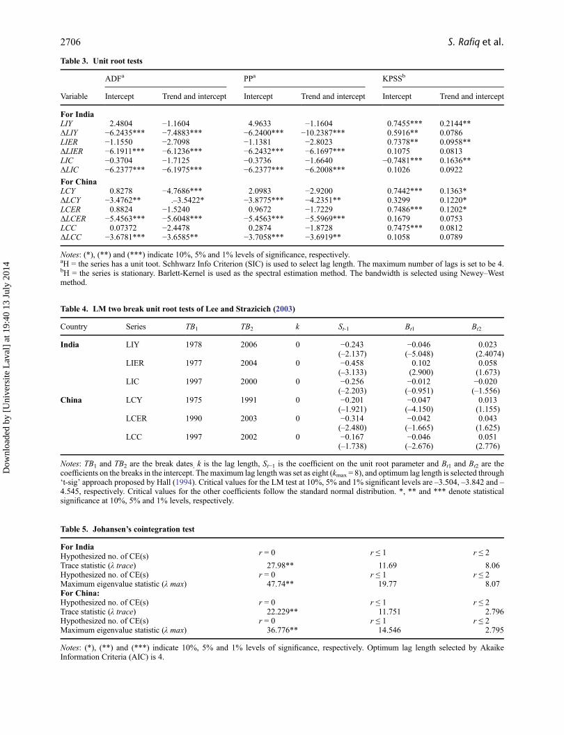
Table 4. LM two break unit root tests of Lee and Strazicich (2003)

Country Series TB1 TB2 k St-1 Bt1 Bt2

India LIY 1978 2006 0 −0.243 −0.046 0.023(–2.137) (–5.048) (2.4074)

LIER 1977 2004 0 −0.458 0.102 0.058(–3.133) (2.900) (1.673)

LIC 1997 2000 0 −0.256 −0.012 −0.020(–2.203) (–0.951) (–1.556)

China LCY 1975 1991 0 −0.201 −0.047 0.013(–1.921) (–4.150) (1.155)

LCER 1990 2003 0 −0.314 −0.042 0.043(–2.480) (–1.665) (1.625)

LCC 1997 2002 0 −0.167 −0.046 0.051(–1.738) (–2.676) (2.776)

Notes: TB1 and TB2 are the break dates, k is the lag length, St−1 is the coefficient on the unit root parameter and Bt1 and Bt2 are thecoefficients on the breaks in the intercept. The maximum lag length was set as eight (kmax = 8), and optimum lag length is selected through‘t-sig’ approach proposed by Hall (1994). Critical values for the LM test at 10%, 5% and 1% significant levels are –3.504, –3.842 and –4.545, respectively. Critical values for the other coefficients follow the standard normal distribution. *, ** and *** denote statisticalsignificance at 10%, 5% and 1% levels, respectively.

Table 5. Johansen’s cointegration test

For IndiaHypothesized no. of CE(s) r = 0 r ≤ 1 r ≤ 2

Trace statistic (λ trace) 27.98** 11.69 8.06Hypothesized no. of CE(s) r = 0 r ≤ 1 r ≤ 2Maximum eigenvalue statistic (λ max) 47.74** 19.77 8.07For China:Hypothesized no. of CE(s) r = 0 r ≤ 1 r ≤ 2Trace statistic (λ trace) 22.229** 11.751 2.796Hypothesized no. of CE(s) r = 0 r ≤ 1 r ≤ 2Maximum eigenvalue statistic (λ max) 36.776** 14.546 2.795

Notes: (*), (**) and (***) indicate 10%, 5% and 1% levels of significance, respectively. Optimum lag length selected by AkaikeInformation Criteria (AIC) is 4.

Table 3. Unit root tests

ADFa PPa KPSSb

Variable Intercept Trend and intercept Intercept Trend and intercept Intercept Trend and intercept

For IndiaLIY 2.4804 −1.1604 4.9633 −1.1604 0.7455*** 0.2144**ΔLIY −6.2435*** −7.4883*** −6.2400*** −10.2387*** 0.5916** 0.0786LIER −1.1550 −2.7098 −1.1381 −2.8023 0.7378** 0.0958**ΔLIER −6.1911*** −6.1236*** −6.2432*** −6.1697*** 0.1075 0.0813LIC −0.3704 −1.7125 −0.3736 −1.6640 −0.7481*** 0.1636**ΔLIC −6.2377*** −6.1975*** −6.2377*** −6.2008*** 0.1026 0.0922

For ChinaLCY 0.8278 −4.7686*** 2.0983 −2.9200 0.7442*** 0.1363*ΔLCY −3.4762** .–3.5422* −3.8775*** −4.2351** 0.3299 0.1220*LCER 0.8824 −1.5240 0.9672 −1.7229 0.7486*** 0.1202*ΔLCER −5.4563*** −5.6048*** −5.4563*** −5.5969*** 0.1679 0.0753LCC 0.07372 −2.4478 0.2874 −1.8728 0.7475*** 0.0812ΔLCC −3.6781*** −3.6585** −3.7058*** −3.6919** 0.1058 0.0789

Notes: (*), (**) and (***) indicate 10%, 5% and 1% levels of significance, respectively.aH = the series has a unit toot. Schhwarz Info Criterion (SIC) is used to select lag length. The maximum number of lags is set to be 4.bH = the series is stationary. Barlett-Kernel is used as the spectral estimation method. The bandwidth is selected using Newey–Westmethod.

2706 S. Rafiq et al.

Dow

nloa

ded

by [

Uni

vers

ite L

aval

] at

19:

40 1

3 Ju

ly 2

014

performed. The results of these ECM-based causality testsin Table 6 show that in the case of India, there is short short-run causality, where renewable energy Granger causes out-put at 1% level of significance. Also, carbon emissionGranger causes both output and renewable energy at 10%level of significance, but there is no short-run causality ofcarbon emission from either output or renewable energy.These short-run results suggest that clean energy is con-tributing to output growth in the Indian economy, but thatgrowth also depends on carbon emission.

The long-run results in Table 6 for India suggest bidirec-tional relationships among variables, which indicate thatcarbon emission, renewable energy and output cause eachother in the long run. The long-run causalities are consistentwith those found by Salim and Rafiq (2012). Overall, theresults for India reveal that renewable energy adoption ispositively contributing to the Indian economy in the shortrun, while increased pressure from emission leads toincreased adoption of renewable energy in the long run,which further enhances development of the country.

In China, a different picture is revealed. In the short run,output causes renewable energy at 5% level of signifi-cance. Hence, economic advances in China contribute tothe renewable energy development. However, no reversedirection in causality is evident. In the long run, it has beenfound that output Granger causes both renewable energy

and carbon emission, while bidirectional causality isfound between carbon emission and renewable energy.Overall, causality in China seems to run from output torenewable energy, with carbon emissions linked in bothcausal directions with renewable energy production.Therefore, in China, it is economic growth that leads toaccelerated adoption of renewable energy, both directlyand through its impact in reducing carbon emissions.

V. Impulse Response Functions

Granger causality tests suggest which variables in themodels have significant impacts on the future values ofeach of the other variables in the system. Nevertheless, theresults do not, by construction, indicate the direction orduration of these impacts. VD and IRFs provide thisinformation. Generalized VD and generalized IRFs arecalculated from the cointegration results using the meth-ods of Koop et al. (1996), and Pesaran and Shin (1998).

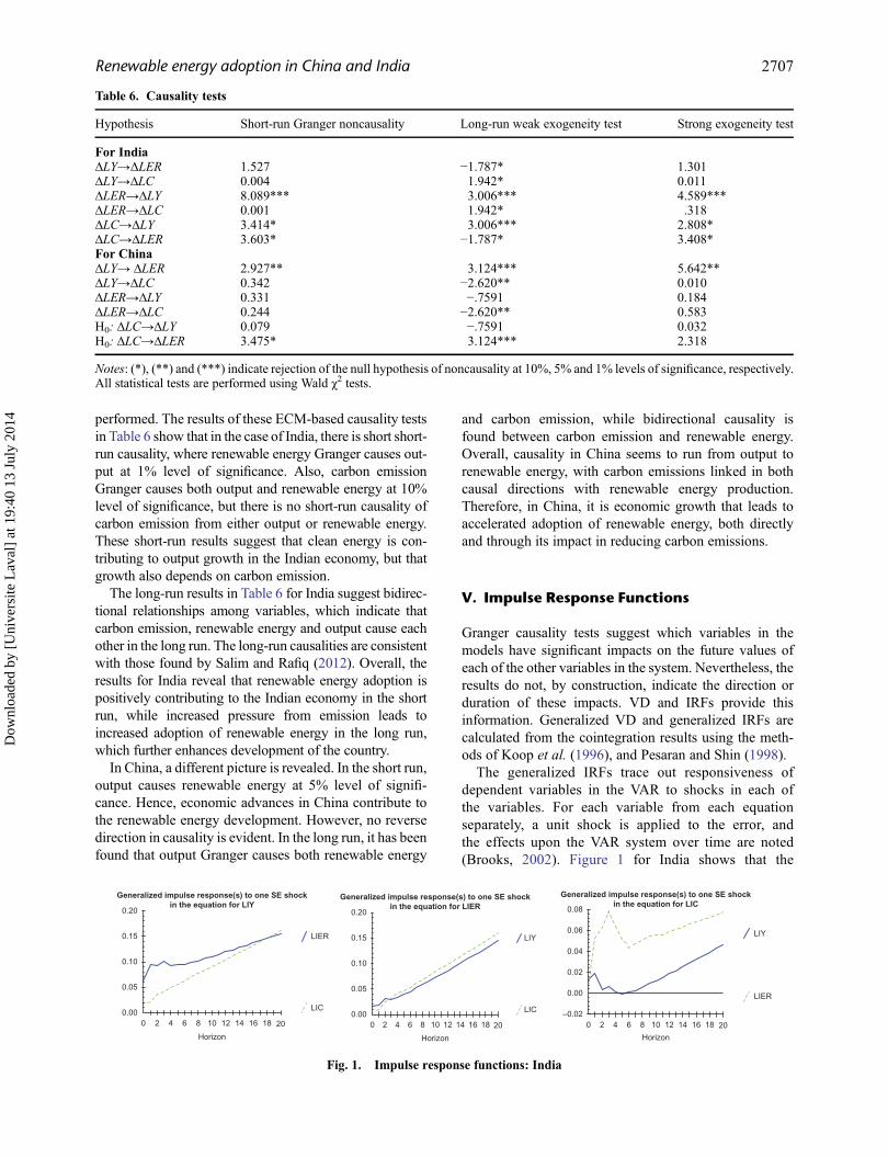
The generalized IRFs trace out responsiveness ofdependent variables in the VAR to shocks in each ofthe variables. For each variable from each equationseparately, a unit shock is applied to the error, andthe effects upon the VAR system over time are noted(Brooks, 2002). Figure 1 for India shows that the

Table 6. Causality tests

Hypothesis Short-run Granger noncausality Long-run weak exogeneity test Strong exogeneity test

For IndiaΔLY→ΔLER 1.527 −1.787* 1.301ΔLY→ΔLC 0.004 1.942* 0.011ΔLER→ΔLY 8.089*** 3.006*** 4.589***ΔLER→ΔLC 0.001 1.942* .318ΔLC→ΔLY 3.414* 3.006*** 2.808*ΔLC→ΔLER 3.603* −1.787* 3.408*For ChinaΔLY→ ΔLER 2.927** 3.124*** 5.642**ΔLY→ΔLC 0.342 −2.620** 0.010ΔLER→ΔLY 0.331 −.7591 0.184ΔLER→ΔLC 0.244 −2.620** 0.583H0: ΔLC→ΔLY 0.079 −.7591 0.032H0: ΔLC→ΔLER 3.475* 3.124*** 2.318

Notes: (*), (**) and (***) indicate rejection of the null hypothesis of noncausality at 10%, 5% and 1% levels of significance, respectively.All statistical tests are performed using Wald χ2 tests.

Generalized impulse response(s) to one SE shockin the equation for LIY

LIER

LIC

Horizon

0.00

0.05

0.10

0.15

0.20

0 4 6 8 10 12 14 16 18 20

Generalized impulse response(s) to one SE shockin the equation for LIER

LIY

LIC

Horizon

0.00

0.05

0.10

0.15

0.20

0 2 4 6 8 10 12 14 16 18 20

Generalized impulse response(s) to one SE shockin the equation for LIC

LIY

LIER

Horizon

–0.02

0.00

0.02

0.04

0.06

0.08

0 4 6 8 10 12 14 16 18 2022

Fig. 1. Impulse response functions: India

Renewable energy adoption in China and India 2707

Dow

nloa

ded

by [

Uni

vers

ite L

aval

] at

19:

40 1

3 Ju

ly 2

014

LIER response from a one unit SE shock in the LIYequation is 10% after 2 years and, after 20 years, itreaches to 15%, while the response of LIC is 2.5%after 2 years, and it increases up to 15% by 20 years.In response to a shock in the equation for LER, analmost continual increase of LIY and LIC is revealed.This supports the causality result that LIER and LICcause LIY. For a shock in the LIC equation, a steadyincrease in both LIY and LIER occur only after someperiods of drift or erratic movement. All these resultsare consistent with the Granger causality result forIndia that there is bi-directional causality among allthe variables.

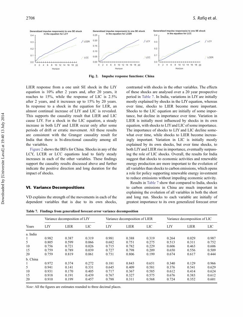
Figure 2 shows the IRFs for China. Shocks in any of theLCY, LCER or LCC equations lead to fairly steadyincreases in each of the other variables. These findingssupport the causality results discussed above and furtherindicate the positive direction and long duration for theimpact of shocks.

VI. Variance Decompositions

VD explains the strength of the movements in each of thedependent variables that is due to its own shocks,

contrasted with shocks in the other variables. The effectsof these shocks are analysed over a 20 year prospectiveperiod in Table 7. In India, variations in LIY are initiallymostly explained by shocks in the LIY equation, whereasover time, shocks to LIER become more important.Shocks to the LIC equation are initially of some impor-tance, but decline in importance over time. Variation inLIER is initially most influenced by shocks in its ownequation, with shocks to LIYand LIC of some importance.The importance of shocks to LIY and LIC decline some-what over time, while shocks to LIER become increas-ingly important. Variation in LIC is initially mostlyexplained by its own shocks, but over time shocks, toboth LIYand LIER rise in importance, eventually surpass-ing the role of LIC shocks. Overall, the results for Indiasuggest that shocks to economic activities and renewableenergy production are more important to the evolution ofall variables than shocks to carbon emissions, which opensa role for policy supporting renewable energy investmentto reduce emissions without impeding economic activity.

Results in Table 7 show that compared to India, shocksto carbon emissions in China are much important inexplaining the evolution of all variables in both the shortand long run. Shocks to each variable are initially ofgreatest importance to its own generalized forecast error

Generalized impulse response(s) to one SE shockin the equation for LCY

LCER

LCC

Horizon

0.0

0.1

0.2

0.3

0.4

0 2 4 6 8 10 12 14 16 18 20

Generalized impulse response(s) to one SE shockin the equation for LCER

LCY

LCC

Horizon

0.00

0.05

0.10

0.15

0.20

0.25

0 2 4 6 8 10 12 14 16 18 20

Generalized impulse response(s) to one SE shockin the equation for LCC

LCY

LCER

Horizon

0.0

0.1

0.2

0.3

0.4

0 2 4 6 8 10 12 14 16 18 20

Fig. 2. Impulse response functions: China

Table 7. Findings from generalized forecast error variance decomposition

Variance decomposition of LIY Variance decomposition of LIER Variance decomposition of LIC

Years LIY LIER LIC LIY LIER LIC LIY LIER LIC

a. India1 0.982 0.387 0.319 0.981 0.388 0.319 0.264 0.029 0.9875 0.805 0.599 0.066 0.682 0.751 0.275 0.513 0.311 0.75210 0.756 0.721 0.026 0.715 0.782 0.229 0.606 0.463 0.60615 0.759 0.789 0.039 0.727 0.798 0.209 0.650 0.556 0.50920 0.759 0.819 0.061 0.731 0.806 0.199 0.674 0.617 0.444

b. China1 0.972 0.374 0.272 0.181 0.843 0.651 0.340 0.129 0.9665 0.941 0.141 0.331 0.645 0.409 0.581 0.376 0.541 0.62910 0.931 0.170 0.405 0.717 0.367 0.585 0.612 0.414 0.62415 0.918 0.191 0.439 0.767 0.327 0.575 0.676 0.383 0.61220 0.910 0.199 0.457 0.788 0.311 0.568 0.724 0.352 0.601

Note: All the figures are estimates rounded to three decimal places.

2708 S. Rafiq et al.

Dow

nloa

ded

by [

Uni

vers

ite L

aval

] at

19:

40 1

3 Ju

ly 2

014

VD, but eventually, shocks to LCY are of greatest impor-tance and shocks to LCC of second importance in eachequation. Shocks to LCER are of much lesser importancein the long run than for either LCY or LCC. Overall, thissuggests that in the case of China, direct action to cutcarbon emissions has been more important than efforts toincrease renewable energy production.

VII. Conclusion

The main objective of this article is to empirically identifythe drivers of renewable energy adoption by examiningthe dynamic relationship among output, carbon emissionsand renewable energy generation in India and China. Thisis done by applying a multivariate vector error-correctionmodel to data from 1972 to 2011. Understanding the pastcausal relationships among these variables can provideguidance as to feasible directions for sustainable futuredevelopment in these rapidly growing economies.

The results of the empirical analysis show that in India,there is statistically significant unidirectional short-runcausality from carbon emission to both renewable energygeneration and output, as well as from renewable energygeneration to output. This suggests that renewable tech-nologies are being used to reduce the detrimental impactsof growing emissions while also helping to boost eco-nomic growth. In the long run, all the variables havebidirectional causality, which points to the inherent inter-dependence of growth, energy production and pollution.The picture of renewable energy implementation in Indianevertheless shows an encouraging trend as renewableenergy technologies are contributing to the sustainabledevelopment of the country.

The results for short-run causalities in China show uni-directional relationships running from output to renewableenergy and from carbon emission to renewable energygeneration. In the long run, the only unidirectional caus-ality is found from output to renewable energy generation,while bidirectional causality is found between carbonemission and renewable energy generation. These resultssuggest that China has already started to commit its sus-tainable development through the adoption of cleanertechnologies linked to both output and carbon emissiongrowth. However, with the huge environmental degrada-tion caused by human activities in the backdrop, furthereffort is required through increasing investment in renew-able energy sources to help mitigate the adverse effects ofcarbon emission while sustaining economic growth.

Acknowledgement

We are grateful to the anonymous referee and the editorof this journal for helpful comments and suggestions

which tremendously improved the quality and presenta-tion of the article. However, we alone are responsible forany error remaining.

Supplemental data

Supplemental data for this article can be accessed here.

References

Ang, J. B. (2007) CO2 emissions, energy consumption, and out-put in France, Energy Policy, 35, 4772–8. doi:10.1016/j.enpol.2007.03.032

Apergis, N. and Payne, J. E. (2009) Energy consumption andeconomic growth in Central America: evidence from apanel cointegration and error correction model, EnergyEconomics, 31, 211–16. doi:10.1016/j.eneco.2008.09.002

Apergis, N. and Tang, C. F. (2013) Is the energy-led growthhypothesis valid? New evidence from a sample of 85 coun-tries, Energy Economics, 38, 24–31. doi:10.1016/j.eneco.2013.02.007

Arouri, M., Youssef, A. B. M., Hatem, C. et al. (2012) Energyconsumption, economic growth and CO2 emissions inMiddle East and North African countries, DiscussionPaper Series No. 6412, Forschungsinstitut zur Zukunft derArbeit, url:nbn:de:101: 1-201206147237.

Asafu-Adjaye, J. (2000) The relationship between energy con-sumption, energy prices and economic growth: time seriesevidence from Asian developing countries, EnergyEconomics, 22, 615–25. doi:10.1016/S0140-9883(00)00050-5

Bloch, H., Rafiq, S. and Salim, R. A. (2012) Coal consumption,CO2 emission and economic growth in China: empiricalevidence and policy responses, Energy Economics, 34,518–28. doi:10.1016/j.eneco.2011.07.014

Brooks, C. (2002) Introductory Econometrics for Finance,Cambridge University Press, Cambridge.

Chandran, V.G.R. and Tang, C. F. (2013) The dynamic linksbetween CO2 emissions, economic growth and coal con-sumption in China and India, Applied Energy, 104, 310–18.doi:10.1016/j.apenergy.2012.10.042

Engle, R. F. and Granger, C. W. J. (1987) Co-integration anderror correction: representation, estimation, and testing,Econometrica, 55, 251. doi:10.2307/1913236.

Fang, Y. (2011) Economic welfare impacts from renewableenergy consumption: the China experience, Renewableand Sustainable Energy Reviews, 15, 5120–28.doi:10.1016/j.rser.2011.07.044.

Ghali, K. H. and El-Sakka, M. I. T. (2004) Energy use and outputgrowth in Canada: a multivariatecointegration analysis,Energy Economics, 26, 225–38. doi:10.1016/S0140-9883(03)00056-2

Ghosh, S. (2002) Electricity consumption and economic growthin India, Energy Policy, 30, 125–29. doi:10.1016/S0301-4215(01)00078-7

Hall, A. D. (1994) Testing for a unit in timeseries with pretestdata based model selection, Journal of Business andEconomic Statistics, 12, 461–70.

Hamit-Haggar, M. (2012) Greenhouse gas emissions, energyconsumption and economic growth: a panel cointegrationanalysis from Canadian industrial sector perspective,Energy Economics, 34, 358–64. doi:10.1016/j.eneco.2011.06.005

Renewable energy adoption in China and India 2709

Dow

nloa

ded

by [

Uni

vers

ite L

aval

] at

19:

40 1

3 Ju

ly 2

014

Johansen, S. (1988) Statistical analysis of cointegration vectors,Journal of Economic Dynamics and Control, 12, 231–54.doi:10.1016/0165-1889(88)90041-3

Johansen, S. (1991) Estimation and hypothesis-testing of coin-tegration vectors in Gaussian vector autoregressive models,Econometrica, 59, 1551–80. doi:10.2307/2938278

Johansen, S. and Juselius, K. (1990) Maximum likelihood esti-mation and inference on cointegration –with applications tothe demand for money, Oxford Bulletin of Economics &Statistics, 52, 169–210. doi:10.1111/j.1468-0084.1990.mp52002003.x

Koop, G., Pesaran, M. H. and Potters, S. M. (1996) Impulseresponse analysis in nonlinear multivariate models, Journalof Econometrics, 74, 119–47. doi:10.1016/0304-4076(95)01753-4

Kraft, J. and Kraft, A. (1978) On the relationship between energyand GNP, Journal of Energy Development, 3, 401–03.

Lee, J. and Strazicich, M. (2003) Minimum Lagrange multiplierunit root test with two structural breaks, Review ofEconomics and Statistics, 85, 1082–89. doi:10.1162/003465303772815961

Liu, X. (2005) Explaining the relationship between CO2 emis-sions and national income – the role of energy consumption,Economics Letters, 87, 325–28. doi:10.1016/j.econlet.2004.09.015.

Ma, H., Oxley, L., Gibson, J. et al. (2008) China’s energyeconomy: technical change, factor demand and interfactor/interfuel substitution, Energy Economics, 30, 2167–83.doi:10.1016/j.eneco.2008.01.010

Masih, A. M. M. and Rumi, M. (1997) On the temporal causalrelationship between energy consumption, real income, andprices: some new evidence from Asian-energy dependentNICs Based on a multivariate cointegration/vector error-correction approach, Journal of Policy Modeling, 19,417–40. doi:10.1016/S0161-8938(96)00063-4

Minihan, E. S. and Wu, Z. (2012) Economic structure andstrategies for greenhouse gas mitigation, EnergyEconomics, 34, 350–7. doi:10.1016/j.eneco.2011.05.011

Narayan, P. K. and Singh, B. (2007) The electricity consumptionand GDP nexus for the Fiji Islands, Energy Economics, 29,1141–50. doi:10.1016/j.eneco.2006.05.018

Oh, W. and Lee, K. (2004) Causal relationship between energyconsumption and GDP revisited: the case of Korea1970–1999, Energy Economics, 26, 51–9. doi:10.1016/S0140-9883(03)00030-6

Pao, H.-T. and Tsai, C.-M. (2010) CO2 emissions, energy con-sumption and economic growth in BRIC countries, EnergyPolicy, 38, 7850–60. doi:10.1016/j.enpol.2010.08.045

Pedroni, P. (2000) Fully modified OLS for heterogeneous coin-tegrated panels, Nonstationary Panels, PanelCointegration, and Dynamic Panels, 15, 93–130.doi:10.1016/S0731-9053(00)15004-2

Perron, P. (1997) Further evidence on breaking trend functions inmacroeconomic variables, Journal of Econometrics, 80,355–85. doi:10.1016/S0304-4076(97)00049-3

Pesaran, H. H. and Shin, Y. (1998) Generalized impulse responseanalysis in linear multivariate models, Economics Letters58, 17–29. doi:10.1016/S0165-1765(97)00214-0

REN21 (2013) Renewables 2013 global status report, RENSecretariate, Paris.

Sadorsky, P. (2009a) Renewable energy consumption, CO2 emis-sions and oil prices in the G7 countries, Energy Economics,31, 456–62. doi:10.1016/j.eneco.2008.12.010

Sadorsky, P. (2009b) Renewable energy consumption andincome in emerging economies, Energy Policy, 37,4021–28. doi:10.1016/j.enpol.2009.05.003.

Salamaliki, P. K. and Venetis, I. A. (2013) Energy consumptionand real GDP in G-7: multi-horizon causality testing in thepresence of capital stock, Energy Economics, 39, 108–21.doi:10.1016/j.eneco.2013.04.010

Salim, R. A. and Bloch, H. (2009) Business expenditures onR&D and trade performances in Australia: is there a link?,Applied Economics, 41, 351–61. doi:10.1080/00036840601007302

Salim, R. A. and Rafiq, S. (2012) Why do some emergingeconomies proactively accelerate the adoption of renewableenergy?, Energy Economics, 34, 1051–57. doi:10.1016/j.eneco.2011.08.015

Sari, R. and Soytas, U. (2007) The growth of income and energyconsumption in six developing countries, Energy Policy,35, 889–98. doi:10.1016/j.enpol.2006.01.021

Stern, D. I. (2000) Amultivariate cointegration analysis of the roleof energy in the US macroeconomy, Energy Economics, 22,267–83. doi:10.1016/S0140-9883(99)00028-6

The World Bank (2007) Growth and CO2 Emissions: How DoDifferent Countries Fare, Environment Department,Washington, DC.

The World Bank (2011) World Development Indicators 2010,World Bank, Washington, DC.

Wolde-Rufael, Y. (2009) Energy consumption and economicgrowth: the experience of African countries revisited,Energy Economics, 31, 217–24. doi:10.1016/j.eneco.2008.11.005

Zamani, M. (2007) Energy consumption and economic activitiesin Iran, Energy Economics, 29, 1135–40. doi:10.1016/j.eneco.2006.04.008

2710 S. Rafiq et al.

Dow

nloa

ded

by [

Uni

vers

ite L

aval

] at

19:

40 1

3 Ju

ly 2

014