The Determinants of Earnings: A Behavioral Approach Samuel ...
The Pakistan Development Review 37 : 3 (Autumn 1998) pp. 251–274
Determinants of Personal Earnings in Pakistan: Findings from the Labour
Force Survey 1993-94
ZAFAR MUEEN NASIR
The paper explores the role of human and non-human capital factors in determining the earnings of workers in Pakistan. The Labour Force Survey data 1993-94, which provides detailed information about workers, has been used for this analysis. Ordinary least squares estimation technique has been utilised for the analysis. The analysis is carried out separately for male and female workers. It is found that in human capital variables, education plays a dominant role in wage determination. In non-human capital factors, occupation and size of the establishments are found to be relevant variables. Other important variables include regional location and technical training. The sample selection bias has been observed for female workers whereas no problem has been observed for male workers, and the bias has been corrected by using the Heckman procedure, though both corrected and uncorrected results are reported. Important conclusions and policy implications are discussed at the end.
I. INTRODUCTION
The distribution of individual earnings is an important issue from the standpoint of public policy. It becomes more important when earnings are skewed among individuals. What is the cause of disparity in earnings? Does it stem from the personal characteristics of individuals or is caused by the labour market characteristics? This and the related questions could easily be answered if the determinants of earnings are known. The focus of the present study is to determine the factors playing a significant role for personal earnings of the individuals. The identification of factors can help design policies not only to improve the economic and social conditions of the individuals but also the overall income distribution.
Zafar Mueen Nasir is Senior Research Economist at the Pakistan Institute of Development Economics, Islamabad.
Author’s Note: In preparing this paper, I benefited from discussions with Dr Ather Maqsood Ahmed and Dr M. Irfan of PIDE. I like to thank them for their generous help. I wish to thank Dr Sarfraz Khan Qureshi for his constant encouragement, and also anonymous referees of this journal for their valuable comments.
Zafar Mueen Nasir 252
A number of studies have estimated the earnings functions for Pakistan [ for example, see Hamdani (1977); Haque (1977); Guisinger et al. (1984); Khan and Irfan (1985); Ashraf and Ashraf (1993); Ahmad and Sirageldin (1994) and others]. But very few have focused on the determinants of personal earnings of the workers. Haque (1977) included socio-economic and human capital variables in the earnings function to explain the earnings differential. Based on Rawalpindi city data, the analysis showed that the human capital factors played a major role in determining individual earnings. It was observed that workers in the formal sector earned either the same income or slightly less than workers of the informal sector. Moreover, male workers earned more than their female counterparts. Shabbir (1994) estimated Mincerian earnings function by utilising the Population, Labour Force, and Migration (PLM) survey data, 1979. The study pointed out that the labour market was not homogeneous and workers in different segments of the labour market received different returns.
Although these studies contribute significantly to understanding the determinants of personal earnings in Pakistan, they, however, suffer from several weaknesses. First, the study by Haque (1977) is confined to only one city which severely restricts its applicability to all Pakistan workers. The study by Shabbir (1994) is limited to male workers, thus ignoring female workers who play a significant role in the Pakistani labour market. Second, none of the studies discussed the issue of sample selection, which leads to bias estimates.1
The present study uses the earnings function approach to examine the determinants of personal earnings of the wage and salaried workers. The paper uses human capital as well as socio-economic (non-human capital) factors to explain the earnings of individuals. The human capital variables are included in the model because of their positive association with the earnings established in Pakistan by earlier studies [Hamdani (1977); Haque (1977); Guisinger et al. (1984); Khan and Irfan (1985) and Shabbir (1994)]. An attempt is also made to account for the gender differences, because a large disparity exists in the earnings of these two groups [Ashraf and Ashraf (1993)]. Other factors such as the occupation and size of the establishment have also been included in the earnings functions because of the existence of labour market segmentation where the returns differ among workers [Khan and Irfan (1985); Shabbir and Khan (1991); Ashraf and Ashraf (1993); Shabbir (1994)]. Thus the present study intends to bridge the gap in literature by providing recent evidence on several aspects of the Pakistani labour market. It utilises nationally representative Labour Force Survey (1993-94), which provides
1Other studies estimated earnings functions for different reasons. For example, Hamdani (1977); Guisinger et al. (1984) and Khan and Irfan (1985) used these functions to calculate the rate of return to education. Ashraf and Ashraf (1993) estimated earnings functions to calculate the male-female earnings gap. Because of their different objectives, these studies ignored many important variables which should have been included in the model. For example, Ashraf and Ashraf (1993) ignored occupations of the workers and size of the establishment. Most of the other studies mentioned above did not account for the distinction between formal and informal sector and employer size.
Determinants of Personal Earnings 253
information on many characteristics of the Pakistani workers. The exclusion of non-wage workers from the model can bias the results if the model is estimated by the ordinary least squares method. The study goes one step forward by providing estimates corrected for sample selection bias using the Heckman (1979) procedure. The paper is structured as follows. Section Two explains the model and its estimation methodology. Section Three deals with the data and its characteristics. Section Four discusses the results. Major findings and policy implications are provided in the concluding section.
II. THEORETICAL FRAMEWORK AND ESTIMATION PROCEDURE
Following Becker (1964) and Mincer (1974), we begin with a simple human capital earning function which indicates that the variation in earnings arises from difference in investment in human capital. As most studies have shown that experience-earnings profiles are usually concave, therefore the quadratic term is used to capture diminishing marginal returns to experience.2 The other adjustments made in the functional form of the earnings equation are described below.
First, as different levels of education impart different skills and earnings, it would be inappropriate to treat schooling as homogenous.3 Thus five levels of education, i.e., 0–4, 5–7, 8–9, 10–13,and degree education are included in the earnings function.
Second, there is a possibility that distinct regional labour markets (urban/rural) may behave differently. In particular, because high-wage urban regions have greater opportunities for jobs and better prospects for higher earnings, therefore it is important to account for regional differences.4
Third, the wage structure may differ because of the existence of segmented labour market (formal and informal sector). According to the conventional microeconomics theory, workers with similar educational levels and measured traits should receive the same wages in the long run. The view is contradicted by the theory of labour market segmentation, which predicts that even in the long run, workers with identical characteristics will not receive the same wage in different labour market segments. This view is supported by many studies, which found that the size of the establishment has a strong effect on wages even when one controls for personal wage and non-wage characteristics of the job.5 The monitoring models of
2Age of the worker is taken as proxy for experience. It is necessary because of many reasons. First, education is available in levels instead of years completed. The widely used procedure to calculate potential experience (age-schooling-6) suggested by Mincer is not possible to calculate due to this reason. Second, as Ashraf and Ashraf (1993) pointed out, the school-going age is not uniform in different parts of the country. Therefore, potential experience is not very useful in the case of Pakistan. Thus, age itself can be as good a proxy for experience as potential experience.
3Evidence from previous research suggests different returns to different levels of education. See, for example, Haque (1977); Khan and Irfan (1985); Shabbir (1992) and Asharf and Ashraf (1993).
4See Shabbir (1994) and Shabbir and Khan (1992). 5Rebitzer and Robinson (1991) examine the effect of employer size on wages in different labour
market segments. See Dickens and Katz (1987) and Krueger and Summers (1988) for studies of industry wage differentials.
Zafar Mueen Nasir 254
labour market segmentation and sociological theories of rent-sharing in the primary sector also support this view. Therefore, to control for the employer size, big and small establishment jobs are separated from the informal sector jobs.
Fourth, because of the divide-and-rule strategies, one can expect firms to favour men over women. According to these models, employers treat one equally productive group of workers better than another by paying a lower wage and thus extract more effort from workers [Roemer (1979); Bowls (1985) and Gintis (1976)]. Furthermore, households assign proportionally larger number of non-work activities to women than men [Juster and Stafford (1991)]. This results in shorter tenures in market jobs and a strong desire for shorter working weeks. Because of these aggregate gender differences, the employers may restrict the access of women to low-paying jobs. Employers may also engage in statistical discrimination against women if, as a group, they have shorter expected tenure than male workers [Bulow and Summers (1986)]. It is, therefore, important to account for the gender differences.
The general form of the equation representing all these variables is presented below.
iiiiii uSOZXwln +β+β+β+β+β= 43210 … … … (1)
In Equation 1, Xi is vector of human capital variables consisting of educational categories, age and its square term, and job training. Zi is the vector of other characteristics such as dummies for regional location and gender groups. Oi is the vector of occupational categories and Si represents the size of the establishments. A complete list of the variables is provided in Table 1.
Before we close this section, a few words regarding the estimation technique are in order. A model like the one presented in Equation 1, if estimated by the ordinary least squares estimation procedure, which excludes non-wage earners, hence truncating the sample, may introduce bias in estimates. As wage-related characteristics also affect labour market participation, it is important to include the non-wage earners in the model for unbiased estimates. A two-step procedure suggested by Heckman (1979), to estimate the wage and labour market participation equations, may reduce sample selection bias from the earnings estimates. In the first step of the Heckman procedure, the inverse of Mill’s ratio, a new regresser, is constructed by estimating a probit model for the probability that an individual is earning. In the second step, earnings are estimated by ordinary least squares using an additional regressor, the inverse of Mill’s ratio. Mathematically, the model can be outlined as:
Let the earnings function be
ii uXYi +β= if Yi > 0 = 0 otherwise … … … … (2)
Determinants of Personal Earnings 255
Table 1
Description of the Variables Used in the Study Variables Description LW Log of monthly earnings of main job at current prices. AGE Current age of the individual. AGESQ Age Squared. LPRIM One if education less than primary including illiterates (zero otherwise). PRIM One if education is between five to seven years (zero otherwise). MID One if education is between eight to nine years (zero otherwise). MAT One if education is between ten to thirteen years (zero otherwise). DEG One if completed degree education (zero otherwise). PRO One if professional, Technical and related workers (zero otherwise). MANG One if Administrative and Managerial workers (zero otherwise). CLERC One if Clerical and related workers (zero otherwise). SALE One if Sales workers (zero otherwise). SERV One if Service workers (zero otherwise). PROD One if Production workers (zero otherwise). AGW One if the profession is agriculture (zero otherwise). SO One if workers of the Small Establishments (zero otherwise). BO One if workers of the Big Establishments (zero otherwise). SEX One if worker is Male (zero otherwise). UR One if worker lives in Urban areas (zero otherwise). WPART One if participate in the wage market (zero otherwise). TT One if completed technical training (zero otherwise). MSP One if married and lives with spouse (zero otherwise). WPART One if participate in the wage market (zero otherwise). DRATIO Dependency ratio = (HS-HE)/HS*
*Here HE and HS stand for earners and total members of the household respectively. where Yi is individual earnings and Xi is a vector of all regressors. Because of the exclusion of non-wage earners from the sample, E (ui) ≠ 0, which violates the important assumption of the ordinary least squares estimation procedure. The inclusion of non-wage earners will modify the model, which becomes
iiii XY ε+δλ+β= … … … … … … (3)
where E(εi)=0 and the new regressor λi is the inverse of Mill’s ratio. The inverse of Mill’s ratio is defined as:
Zafar Mueen Nasir 256
⎭⎬⎫
⎩⎨⎧
δβ
⎭⎬⎫
⎩⎨⎧
δβ
=λi
i
i XF
Xf
… … … … … … (4)
where f is the density and F is the probability distribution function of the standard
normal distribution. Both functions are evaluated at δ
β iX . To overcome the
estimation problem because of the λi , an unknown, Heckman suggested using a censoring indicator in the first step. For this purpose, a dependent dummy of wage participation Zi is considered. This variable includes both wage and non-wage earners. It is defined as
Zi = 1 if Yi > 0 = 0 if Yi ≤ 0 … … … … … (5)
Information on this variable is available. The probit model to be estimated by the maximum likelihood estimation procedure is
)(11)0(
)()1(
ii
i
ii
i
XFXFZP
XFXFZP
ω−=⎭⎬⎫
⎩⎨⎧
δβ
−==
ω=⎭⎬⎫
⎩⎨⎧
δβ
==
which provides estimates of ω. Once ω is estimated, by substitution we obtain λi, which is
)()(
XFXf i
i ωω
=λ … … … … … … (7)
As λi , the inverse of Mill’s ratio can be derived in the first step, the estimation of Equation 4 in the second step, by OLS results in unbiased and consistent estimates.
III. DATA CHARACTERISTICS
The data used in this paper are drawn from the Labour Force Survey (LFS) 1993-94. It is a regular feature of the Federal Bureau of Statistics (FBS) since July, 1963. These data provides comprehensive information not only on the unemployed persons but also on many characteristics of employed persons. The information on earnings, age, education levels, sex, marital status, regions, employer size, occupation, and employment status is particularly important for this study. The
… … … … (6)
Determinants of Personal Earnings 257
unique aspect of the Labour Force Survey data is that it separates regular wage employees from casual paid workers, paid non-family apprentices, and those who are working at piece rate.6 This distinction enabled us to separate regular wage employees from irregular wage workers. The other useful information in the Labour Force Survey is about the place of work. This information helped us to separate the formal sector from the informal sector. Additionally, from the information given, we can distinguish small establishments from the big ones. Another feature of the data set is that it has detailed information about earnings. It separates cash payments from non-cash payments and the bonuses from regular salary. Moreover, this data set is used for the first time to estimate earnings functions.
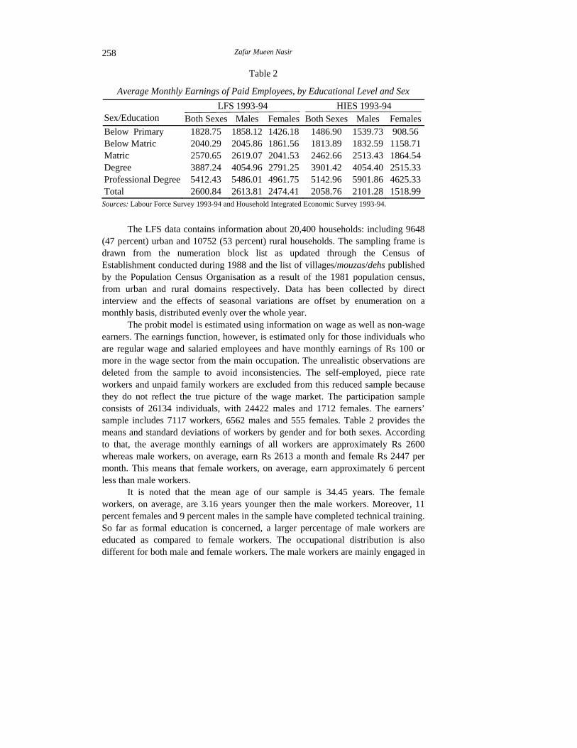
The other commonly used comparable data source is the Household Integrated Economic Survey (HIES). Although it provides information about many characteristics of individuals but lacks such details as the LFS provides. The Labour Force Survey is exclusively designed to explore the Pakistani labour market, whereas the HIES has its main focus on gathering information on income and expenditure of the household. Both data sets are compared in Table 2, which presents average monthly earnings of paid employees by education. This comparison is carried out for both sexes, and for males and females, separately.
The comparison shows that except for degree-holders, workers in the LFS with different educational backgrounds receive much higher wages relative to the workers represented in the HIES. It is also noted that the HIES data represent a higher percentage of female workers having ten or less years of schooling (i.e., 76 percent in the HIES as compared to 46 percent in the LFS). This is one of the reasons for lower female-male earnings ratio in the HIES relative to the LFS. To further explore the low female-male earnings ratio in the HIES as compared to the LFS, we disaggregated both data sets into formal and informal sectors of employment. This was done due to the fact that the earnings in the informal sector are lower than in the formal sector [Ghayur (1993)]. It is found that the representation of informal sector workers in the HIES is higher than in the LFS data, i.e., 59 percent in the HIES as compared to 53 percent in the LFS. Furthermore, it is found that a higher percentage of female workers in the HIES (65 percent) relative to the LFS (59 percent) work in the informal sector. The average earnings of these female workers are found to be Rs 928.92 and Rs 1596.27 in the HIES and the LFS respectively. This may be another reason for lower female-male earnings ratio.
The comparison of these two data sets leads us to believe that the earnings of workers in the HIES are understated relative to the LFS data. The analysis based on the HIES data may lead us to biased estimates, therefore we used the LFS data for this study. Some important details of the LFS are provided below.
6The list of irregular workers included those who are paid when the service has been performed.
Zafar Mueen Nasir 258
Table 2
Average Monthly Earnings of Paid Employees, by Educational Level and Sex LFS 1993-94 HIES 1993-94
Sex/Education Both Sexes Males Females Both Sexes Males Females Below Primary 1828.75 1858.12 1426.18 1486.90 1539.73 908.56 Below Matric 2040.29 2045.86 1861.56 1813.89 1832.59 1158.71 Matric 2570.65 2619.07 2041.53 2462.66 2513.43 1864.54 Degree 3887.24 4054.96 2791.25 3901.42 4054.40 2515.33 Professional Degree 5412.43 5486.01 4961.75 5142.96 5901.86 4625.33 Total 2600.84 2613.81 2474.41 2058.76 2101.28 1518.99
Sources: Labour Force Survey 1993-94 and Household Integrated Economic Survey 1993-94.
The LFS data contains information about 20,400 households: including 9648
(47 percent) urban and 10752 (53 percent) rural households. The sampling frame is drawn from the numeration block list as updated through the Census of Establishment conducted during 1988 and the list of villages/mouzas/dehs published by the Population Census Organisation as a result of the 1981 population census, from urban and rural domains respectively. Data has been collected by direct interview and the effects of seasonal variations are offset by enumeration on a monthly basis, distributed evenly over the whole year.
The probit model is estimated using information on wage as well as non-wage earners. The earnings function, however, is estimated only for those individuals who are regular wage and salaried employees and have monthly earnings of Rs 100 or more in the wage sector from the main occupation. The unrealistic observations are deleted from the sample to avoid inconsistencies. The self-employed, piece rate workers and unpaid family workers are excluded from this reduced sample because they do not reflect the true picture of the wage market. The participation sample consists of 26134 individuals, with 24422 males and 1712 females. The earners’ sample includes 7117 workers, 6562 males and 555 females. Table 2 provides the means and standard deviations of workers by gender and for both sexes. According to that, the average monthly earnings of all workers are approximately Rs 2600 whereas male workers, on average, earn Rs 2613 a month and female Rs 2447 per month. This means that female workers, on average, earn approximately 6 percent less than male workers.
It is noted that the mean age of our sample is 34.45 years. The female workers, on average, are 3.16 years younger then the male workers. Moreover, 11 percent females and 9 percent males in the sample have completed technical training. So far as formal education is concerned, a larger percentage of male workers are educated as compared to female workers. The occupational distribution is also different for both male and female workers. The male workers are mainly engaged in
Determinants of Personal Earnings 259
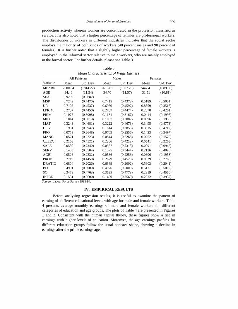
production activity whereas women are concentrated in the profession classified as service. It is also noted that a higher percentage of females are professional workers. The distribution of workers in different industries indicates that the social sector employs the majority of both kinds of workers (48 percent males and 90 percent of females). It is further noted that a slightly higher percentage of female workers is employed in the informal sector relative to male workers, who are mainly employed in the formal sector. For further details, please see Table 3.
Table 3 Mean Characteristics of Wage Earners
All Pakistan Males Females Variable Mean Std. Dev Mean Std. Dev Mean Std. Dev MEARN 2600.84 (1814.22) 2613.81 (1807.25) 2447.41 (1889.56) AGE 34.46 (11.54) 34.70 (11.57) 31.51 (10.81) SEX 0.9200 (0.2682) – – – – MSP 0.7242 (0.4470) 0.7415 (0.4378) 0.5189 (0.5001) UR 0.7103 (0.4537) 0.6980 (0.4592) 0.8559 (0.3516) LPRIM 0.2737 (0.4458) 0.2767 (0.4474) 0.2378 (0.4261) PRIM 0.1075 (0.3098) 0.1131 (0.3167) 0.0414 (0.1995) MID 0.1014 (0.3019) 0.1067 (0.3087) 0.0396 (0.1953) MAT 0.3243 (0.4681) 0.3222 (0.4673) 0.3495 (0.4773) DEG 0.1931 (0.3947) 0.1814 (0.3853) 0.3315 (0.4712) PRO 0.0759 (0.2648) 0.0703 (0.2556) 0.1423 (0.3497) MANG 0.0521 (0.2223) 0.0544 (0.2268) 0.0252 (0.1570) CLERC 0.2168 (0.4121) 0.2306 (0.4212) 0.0541 (0.2263) SALE 0.0530 (0.2240) 0.0567 (0.2313) 0.0091 (0.0945) SERV 0.1433 (0.3504) 0.1375 (0.3444) 0.2126 (0.4095) AGRI 0.0526 (0.2232) 0.0536 (0.2253) 0.0396 (0.1953) PROD 0.2719 (0.4450) 0.2879 (0.4528) 0.0829 (0.2760) DRATIO 0.6804 (0.2026) 0.6889 (0.2002) 0.5803 (0.2041) BO 0.4991 (0.5000) 0.4976 (0.5000) 0.5171 (0.5002) SO 0.3478 (0.4763) 0.3525 (0.4778) 0.2919 (0.4550) INFOR 0.1531 (0.3600) 0.1499 (0.3569) 0.2922 (0.3932)
Source: Labour Force Survey 1993-94.
IV. EMPIRICAL RESULTS
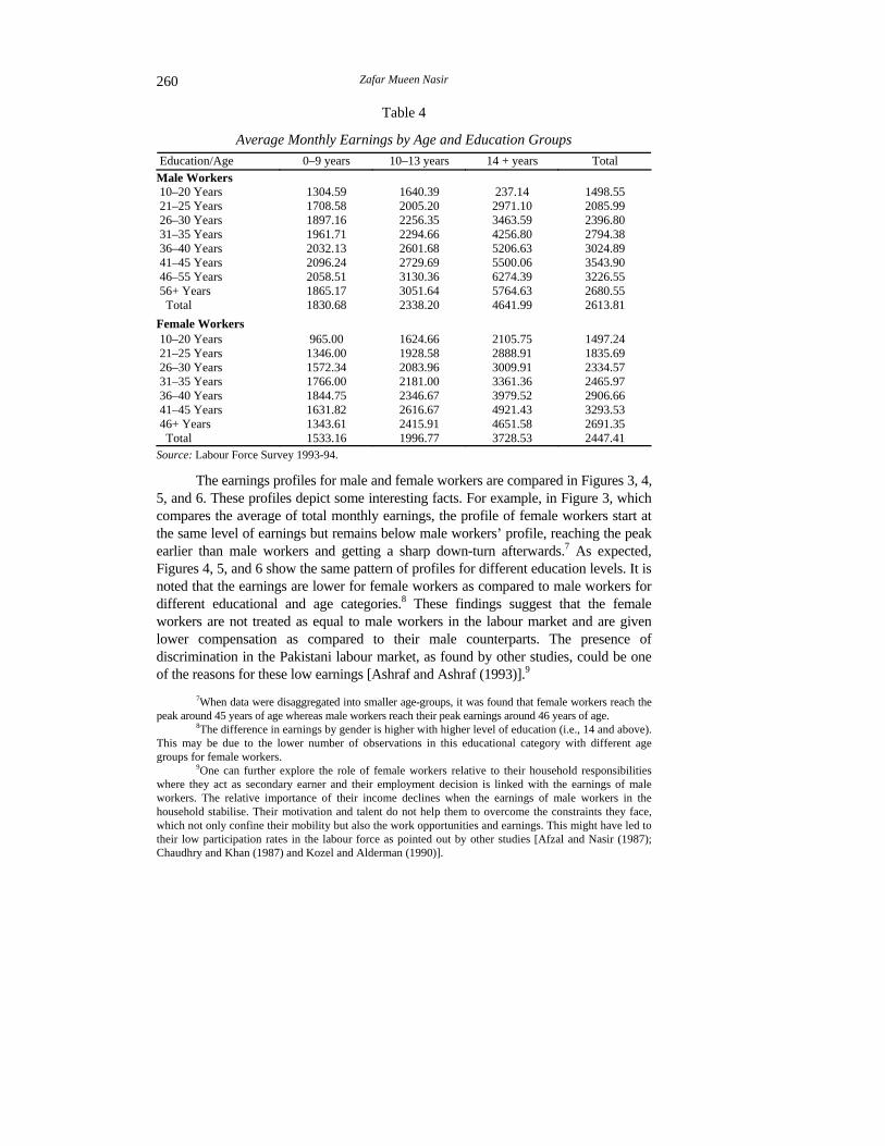
Before analysing regression results, it is useful to examine the pattern of earning of different educational levels with age for male and female workers. Table 4 presents average monthly earnings of male and female workers for different categories of education and age groups. The plots of Table 4 are presented in Figures 1 and 2. Consistent with the human capital theory, these figures show a rise in earnings with higher levels of education. Moreover, the age earnings profiles for different education groups follow the usual concave shape, showing a decline in earnings after the prime earnings age.
Zafar Mueen Nasir 260
Table 4
Average Monthly Earnings by Age and Education Groups Education/Age 0–9 years 10–13 years 14 + years Total
Male Workers 10–20 Years 1304.59 1640.39 237.14 1498.55 21–25 Years 1708.58 2005.20 2971.10 2085.99 26–30 Years 1897.16 2256.35 3463.59 2396.80 31–35 Years 1961.71 2294.66 4256.80 2794.38 36–40 Years 2032.13 2601.68 5206.63 3024.89 41–45 Years 2096.24 2729.69 5500.06 3543.90 46–55 Years 2058.51 3130.36 6274.39 3226.55 56+ Years 1865.17 3051.64 5764.63 2680.55 Total 1830.68 2338.20 4641.99 2613.81
Female Workers 10–20 Years 965.00 1624.66 2105.75 1497.24 21–25 Years 1346.00 1928.58 2888.91 1835.69 26–30 Years 1572.34 2083.96 3009.91 2334.57 31–35 Years 1766.00 2181.00 3361.36 2465.97 36–40 Years 1844.75 2346.67 3979.52 2906.66 41–45 Years 1631.82 2616.67 4921.43 3293.53 46+ Years 1343.61 2415.91 4651.58 2691.35 Total 1533.16 1996.77 3728.53 2447.41
Source: Labour Force Survey 1993-94.
The earnings profiles for male and female workers are compared in Figures 3, 4, 5, and 6. These profiles depict some interesting facts. For example, in Figure 3, which compares the average of total monthly earnings, the profile of female workers start at the same level of earnings but remains below male workers’ profile, reaching the peak earlier than male workers and getting a sharp down-turn afterwards.7 As expected, Figures 4, 5, and 6 show the same pattern of profiles for different education levels. It is noted that the earnings are lower for female workers as compared to male workers for different educational and age categories.8 These findings suggest that the female workers are not treated as equal to male workers in the labour market and are given lower compensation as compared to their male counterparts. The presence of discrimination in the Pakistani labour market, as found by other studies, could be one of the reasons for these low earnings [Ashraf and Ashraf (1993)].9
7When data were disaggregated into smaller age-groups, it was found that female workers reach the peak around 45 years of age whereas male workers reach their peak earnings around 46 years of age.
8The difference in earnings by gender is higher with higher level of education (i.e., 14 and above). This may be due to the lower number of observations in this educational category with different age groups for female workers.
9One can further explore the role of female workers relative to their household responsibilities where they act as secondary earner and their employment decision is linked with the earnings of male workers. The relative importance of their income declines when the earnings of male workers in the household stabilise. Their motivation and talent do not help them to overcome the constraints they face, which not only confine their mobility but also the work opportunities and earnings. This might have led to their low participation rates in the labour force as pointed out by other studies [Afzal and Nasir (1987); Chaudhry and Khan (1987) and Kozel and Alderman (1990)].

Fig. 1. Earning Profile of Male Workers by Age and Education.
Fig. 2. Earning Profile of Female Workers by Age and Education.
0
1000
2000
3000
4000
5000
6000
7000
10-20 y 21-25 y 26-30 y 31-35 y 36-40 y 41-45 y 46-55 y 56+
Age (years)
Ave
rage
Mon
thly
Ear
ning
(Rs)
0-9 years 10-13 years 14 + years
0
1000
2000
3000
4000
5000
6000
10-20 y 21-25 y 26-30 y 31-35 y 36-40 y 41-45 y 46-55 yAge (years)
Ave
rage
Mon
thly
Ear
ning
(Rs)
0-9 years 10-13 years 14 + years
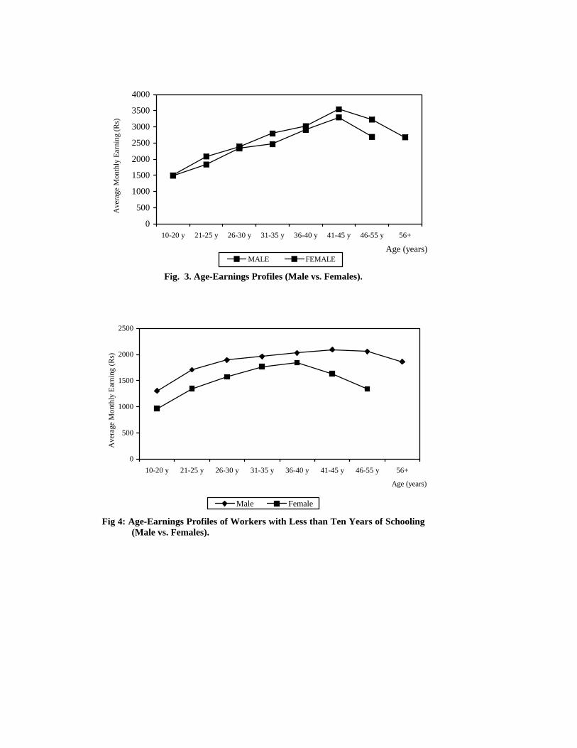
Fig. 3. Age-Earnings Profiles (Male vs. Females).
Fig 4: Age-Earnings Profiles of Workers with Less than Ten Years of Schooling (Male vs. Females).
0
500
1000
1500
2000
2500
3000
3500
4000
10-20 y 21-25 y 26-30 y 31-35 y 36-40 y 41-45 y 46-55 y 56+
Age (years)
Ave
rage
Mon
thly
Ear
ning
(Rs)
MALE FEMALE
0
500
1000
1500
2000
2500
10-20 y 21-25 y 26-30 y 31-35 y 36-40 y 41-45 y 46-55 y 56+
Age (years)
Ave
rage
Mon
thly
Ear
ning
(Rs)
Male Female
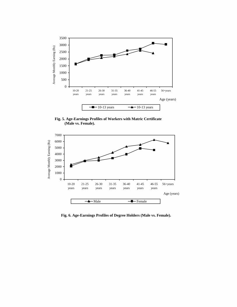
Fig. 5. Age-Earnings Profiles of Workers with Matric Certificate
(Male vs. Female).
Fig. 6. Age-Earnings Profiles of Degree Holders (Male vs. Female).
0
500
1000
1500
2000
2500
3000
3500
10-20years
21-25years
26-30years
31-35years
36-40years
41-45years
46-55years
56+years
Age (years)
Ave
rage
Mon
thly
Ear
ning
(Rs)
10-13 years 10-13 years
0
1000
2000
3000
4000
5000
6000
7000
10-20years
21-25years
26-30years
31-35years
36-40years
41-45years
46-55years
56+years
Age (years)
Ave
rage
Mon
thly
Ear
ning
(Rs)
Male Female
Zafar Mueen Nasir 264
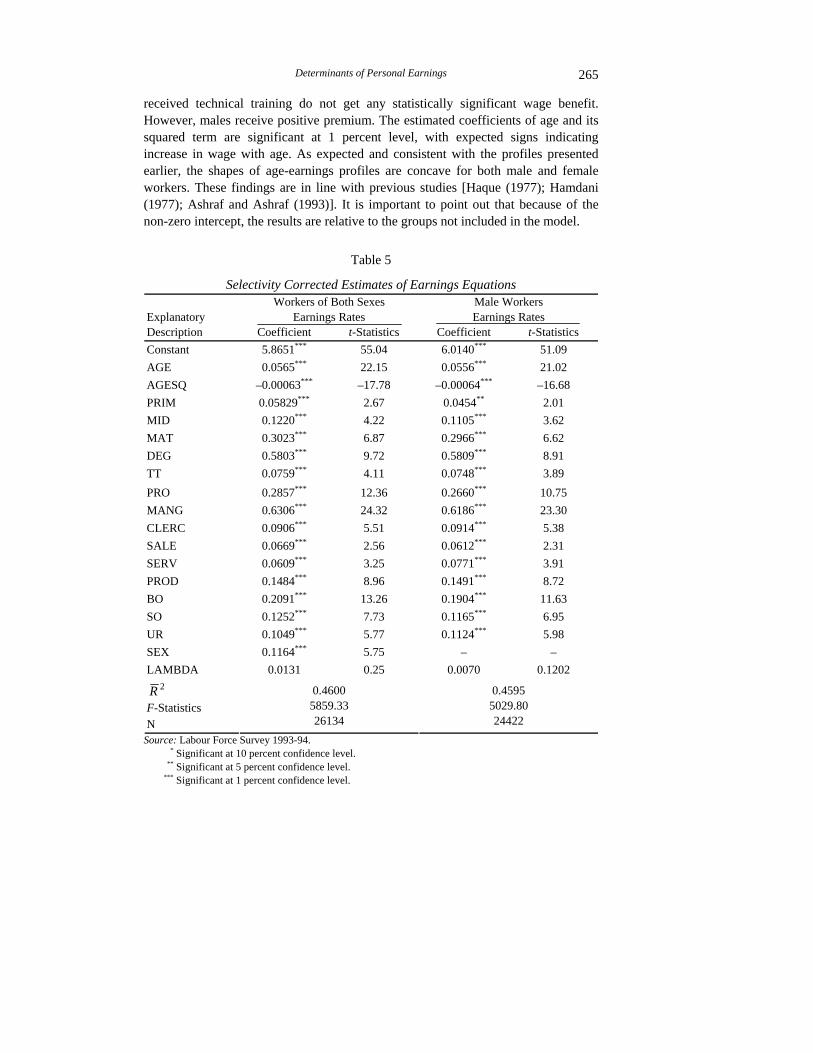
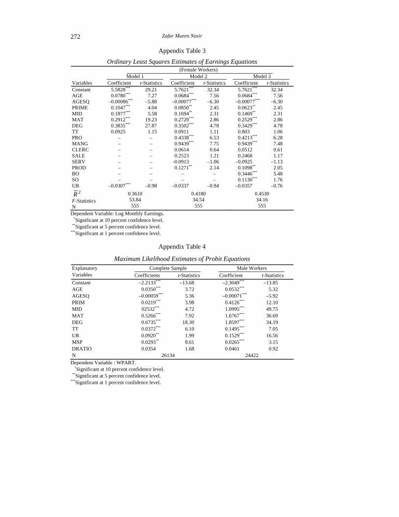
The wage functions estimated by the maximum likelihood method using probit estimates of wage participation are presented in Tables 5 and 6 for all, male and female workers respectively. Models with step-wise inclusion of different traits of workers are presented in Appendix. The wage estimates indicate that human capital variables explain a substantial portion of the variation in earnings. Among the important determinants of productivity, age (proxy for experience) and education are crucial. Consistent with the human capital theory, earnings in the present case are an increasing function of education. A partial model that includes only human capital variables explains 38 percent of the variation for the complete sample, whereas such a model explains 39 percent for male workers and 36 percent for female workers. Inclusion of dummy variables for occupation and size of the firm explains an additional 8 percent of variation in the main regression models.10 Moreover, judged by the F-statistics, the overall performance of the models is also good. Since the dependent variable “monthly earnings” is in logs, the coefficients of independent variables are interpreted as percentage.
The sample selectivity revealed by the inverse of Mill’s ratio for the complete sample and the sample for the male workers turned out to be statistically insignificant for variable LAMDA. This suggests that there is no problem of selection for male workers as those who opt wage sector employment do not earn differently from those who choose to work in the non-wage sector. In contrast to male workers, there is a strong evidence of selectivity among female workers. A negative and significant LAMDA indicates positive selection bias for females’ earnings in the wage sector. This implies that those who participate in the labour market belong to a non-random sample of the population. The endogenous nature of decision rule is clearly evident for women as compared to their male counterparts. Women who choose wage sector employment earn more than average non-wage sector earners. This also suggests that females who choose wage sector employment have above-average abilities; they are highly motivated, and are careful in their decision process.
As expected, the coefficients on schooling for males and females are positive and statistically significant for all levels. The premiums for primary, middle, and secondary level are 8 percent, 15 percent, and approximately 30 percent, respectively, for female workers relative to the base group.11 It is noted that the highest returns are associated with degree education. A similar pattern is observed for male workers. These results are consistent with other studies, which reported rising trend in earnings with the levels of education involved [Ashraf and Ashraf (1993); Kozel and Alderman (1990); and Shabbir (1992)]. Female workers who
10This 2R is quite high for our model because usually it is low for cross-section estimates. 11The returns are calculated by taking the anti-log of 0.0757 (estimated coefficient of PRIM) and
subtracting one. To convert into percentage, we multiply the value by 100. For more details, see Gujarati (1988), p. 149.
Determinants of Personal Earnings 265
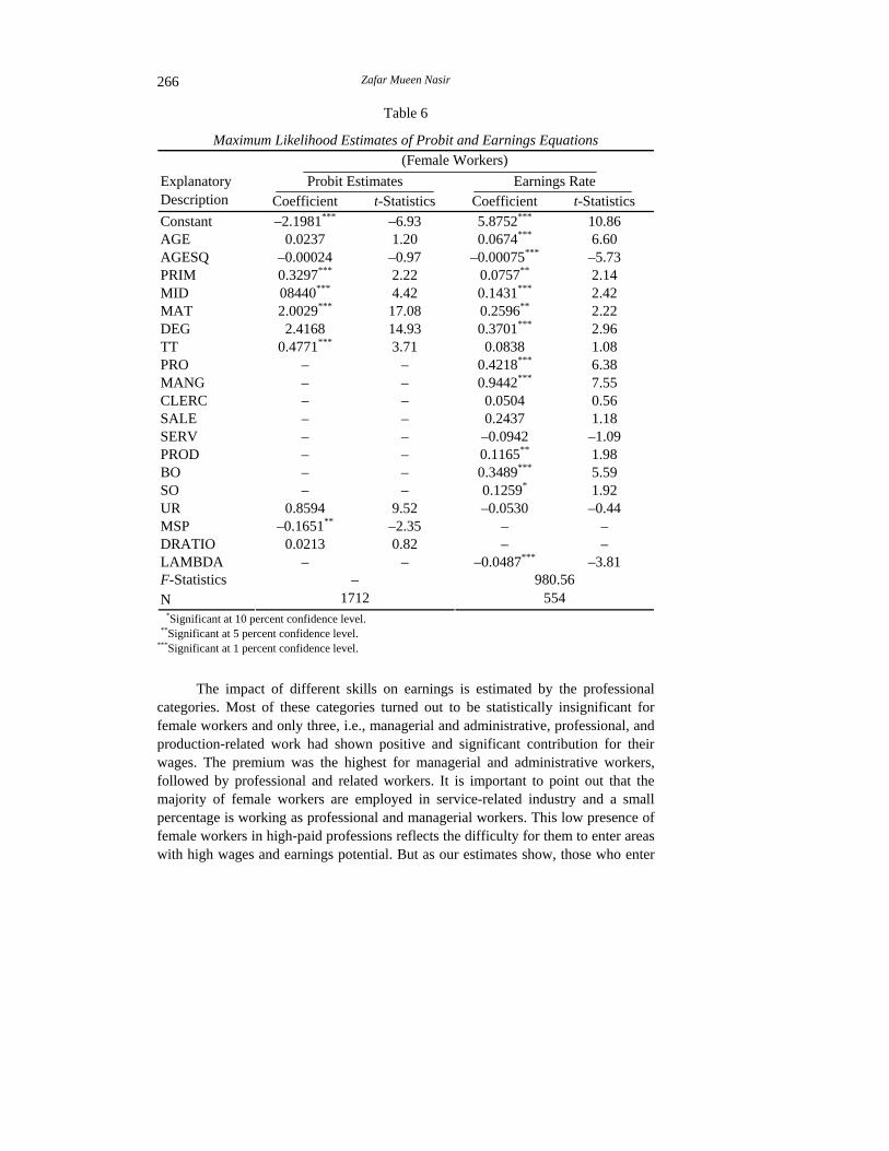
received technical training do not get any statistically significant wage benefit. However, males receive positive premium. The estimated coefficients of age and its squared term are significant at 1 percent level, with expected signs indicating increase in wage with age. As expected and consistent with the profiles presented earlier, the shapes of age-earnings profiles are concave for both male and female workers. These findings are in line with previous studies [Haque (1977); Hamdani (1977); Ashraf and Ashraf (1993)]. It is important to point out that because of the non-zero intercept, the results are relative to the groups not included in the model.
Table 5
Selectivity Corrected Estimates of Earnings Equations Workers of Both Sexes Male Workers Explanatory Earnings Rates Earnings Rates Description Coefficient t-Statistics Coefficient t-Statistics Constant 5.8651*** 55.04 6.0140*** 51.09 AGE 0.0565*** 22.15 0.0556*** 21.02 AGESQ –0.00063*** –17.78 –0.00064*** –16.68 PRIM 0.05829*** 2.67 0.0454** 2.01 MID 0.1220*** 4.22 0.1105*** 3.62 MAT 0.3023*** 6.87 0.2966*** 6.62 DEG 0.5803*** 9.72 0.5809*** 8.91 TT 0.0759*** 4.11 0.0748*** 3.89 PRO 0.2857*** 12.36 0.2660*** 10.75 MANG 0.6306*** 24.32 0.6186*** 23.30 CLERC 0.0906*** 5.51 0.0914*** 5.38 SALE 0.0669*** 2.56 0.0612*** 2.31 SERV 0.0609*** 3.25 0.0771*** 3.91 PROD 0.1484*** 8.96 0.1491*** 8.72 BO 0.2091*** 13.26 0.1904*** 11.63 SO 0.1252*** 7.73 0.1165*** 6.95 UR 0.1049*** 5.77 0.1124*** 5.98 SEX 0.1164*** 5.75 – – LAMBDA 0.0131 0.25 0.0070 0.1202
2R F-Statistics N
0.4600 5859.33 26134
0.4595 5029.80 24422
Source: Labour Force Survey 1993-94. * Significant at 10 percent confidence level. ** Significant at 5 percent confidence level. *** Significant at 1 percent confidence level.
Zafar Mueen Nasir 266
Table 6
Maximum Likelihood Estimates of Probit and Earnings Equations (Female Workers)
Probit Estimates Earnings Rate Explanatory Description Coefficient t-Statistics Coefficient t-Statistics Constant –2.1981*** –6.93 5.8752*** 10.86 AGE 0.0237 1.20 0.0674*** 6.60 AGESQ –0.00024 –0.97 –0.00075*** –5.73 PRIM 0.3297*** 2.22 0.0757** 2.14 MID 08440*** 4.42 0.1431*** 2.42 MAT 2.0029*** 17.08 0.2596** 2.22 DEG 2.4168 14.93 0.3701*** 2.96 TT 0.4771*** 3.71 0.0838 1.08 PRO – – 0.4218*** 6.38 MANG – – 0.9442*** 7.55 CLERC – – 0.0504 0.56 SALE – – 0.2437 1.18 SERV – – –0.0942 –1.09 PROD – – 0.1165** 1.98 BO – – 0.3489*** 5.59 SO – – 0.1259* 1.92 UR 0.8594 9.52 –0.0530 –0.44 MSP –0.1651** –2.35 – – DRATIO 0.0213 0.82 – – LAMBDA – – –0.0487*** –3.81 F-Statistics N
– 1712
980.56 554
*Significant at 10 percent confidence level. **Significant at 5 percent confidence level. ***Significant at 1 percent confidence level.
The impact of different skills on earnings is estimated by the professional
categories. Most of these categories turned out to be statistically insignificant for female workers and only three, i.e., managerial and administrative, professional, and production-related work had shown positive and significant contribution for their wages. The premium was the highest for managerial and administrative workers, followed by professional and related workers. It is important to point out that the majority of female workers are employed in service-related industry and a small percentage is working as professional and managerial workers. This low presence of female workers in high-paid professions reflects the difficulty for them to enter areas with high wages and earnings potential. But as our estimates show, those who enter
Determinants of Personal Earnings 267
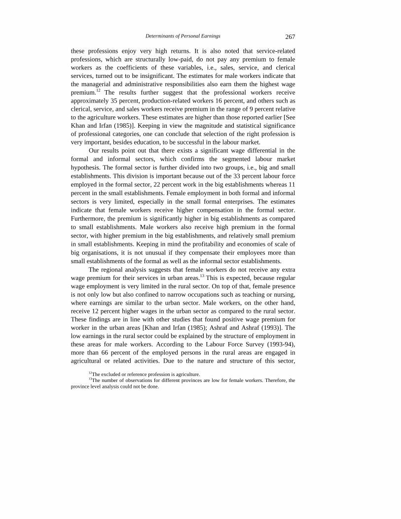
these professions enjoy very high returns. It is also noted that service-related professions, which are structurally low-paid, do not pay any premium to female workers as the coefficients of these variables, i.e., sales, service, and clerical services, turned out to be insignificant. The estimates for male workers indicate that the managerial and administrative responsibilities also earn them the highest wage premium.12 The results further suggest that the professional workers receive approximately 35 percent, production-related workers 16 percent, and others such as clerical, service, and sales workers receive premium in the range of 9 percent relative to the agriculture workers. These estimates are higher than those reported earlier [See Khan and Irfan (1985)]. Keeping in view the magnitude and statistical significance of professional categories, one can conclude that selection of the right profession is very important, besides education, to be successful in the labour market.
Our results point out that there exists a significant wage differential in the formal and informal sectors, which confirms the segmented labour market hypothesis. The formal sector is further divided into two groups, i.e., big and small establishments. This division is important because out of the 33 percent labour force employed in the formal sector, 22 percent work in the big establishments whereas 11 percent in the small establishments. Female employment in both formal and informal sectors is very limited, especially in the small formal enterprises. The estimates indicate that female workers receive higher compensation in the formal sector. Furthermore, the premium is significantly higher in big establishments as compared to small establishments. Male workers also receive high premium in the formal sector, with higher premium in the big establishments, and relatively small premium in small establishments. Keeping in mind the profitability and economies of scale of big organisations, it is not unusual if they compensate their employees more than small establishments of the formal as well as the informal sector establishments.
The regional analysis suggests that female workers do not receive any extra wage premium for their services in urban areas.13 This is expected, because regular wage employment is very limited in the rural sector. On top of that, female presence is not only low but also confined to narrow occupations such as teaching or nursing, where earnings are similar to the urban sector. Male workers, on the other hand, receive 12 percent higher wages in the urban sector as compared to the rural sector. These findings are in line with other studies that found positive wage premium for worker in the urban areas [Khan and Irfan (1985); Ashraf and Ashraf (1993)]. The low earnings in the rural sector could be explained by the structure of employment in these areas for male workers. According to the Labour Force Survey (1993-94), more than 66 percent of the employed persons in the rural areas are engaged in agricultural or related activities. Due to the nature and structure of this sector,
12The excluded or reference profession is agriculture. 13The number of observations for different provinces are low for female workers. Therefore, the
province level analysis could not be done.
Zafar Mueen Nasir 268
earnings are low and uncertain. This survey reports that 53 percent of the rural employed persons earn up to Rs 1500 per month. It is also found that in rural areas, a majority (26 percent) of employees is daily wage earner. This provides a solid reason for lower earnings in the rural sector as compared to the urban areas.
V. CONCLUSIONS AND POLICY IMPLICATIONS
The study is carried out to determine the factors playing an important role in the personal earnings of regular wage employees. Our complete sample, which includes both male and female workers, was not different from the workers randomly selected from the population. However, when it was disaggregated on gender basis, we found the selectivity problem for female workers. This suggested that the female workers in our sample had characteristics different from those who worked in the non-wage sector. The reported results are adjusted by the Heckman procedure for the bias arising from this sample selectivity. The main findings are summarised below.
Our results suggested that the labour market was structured differently for male and female workers. The difference arose because of individual’s regional location, selection of occupation, industry association, and personal characteristics.
Education is found to be an important determinant of the earnings for female as well as male workers; it enhances their productivity, and thus earnings. The earnings were the highest for those having a college/university education.
The selection of profession was also an important determinant of earnings for both male and female workers. It was found that females classified as professional or managerial and administrative workers received much higher compensation as compared to the other professions. A statistically significant wage premium for male workers was found for all professional categories.
It was observed that compensation in the formal sector was higher than in the informal sector. Size of the establishment in the formal sector, however, was important for female workers. They received significant wage premium in the big establishments whereas no extra premium was found in the small establishments. Although the earnings’ premium for male workers was higher in the big establishments, small establishment workers also received wage premium. The regional location was found to be less important for female workers. However, male workers received higher compensation in the urban areas as compared to the rural sector. These findings point out the segmentation of the labour market for primary and secondary jobs.
The improvement in the economic and social conditions of low-paid groups, particularly female workers, require comprehensive policy formulation. Some policy measures are suggested below. These measures can reduce the earnings differential and income inequality among workers by providing them opportunities to enter the primary sector where earnings potential is higher.
Determinants of Personal Earnings 269
To reduce the regional earnings differential, it is suggested that professions other than agriculture be promoted in the rural areas. Moreover, agro-based industries such as sugar, preservation and canning of fruits and vegetables, and ginning should be established in the rural areas. The cottage industry should also be given due importance in the rural areas. There is a dire need to develop the infrastructure in rural areas to attract investment. These steps will be very helpful in raising earnings of the rural area workers and in reducing the earnings gap. It is also recommended to give more incentives to labour-intensive industries so as to absorb unemployed youth.
Participation of females in all occupations should also be encouraged by providing them with the opportunity to enhance their human capital endowment, i.e., education and training in different fields. In addition to that, the informal sector needs to be restructured and employment opportunities for female workers should be increased. At present, female participation in this sector is very low because of its unsuitability for female employment. The restructuring of this sector by promoting female entrepreneureship in female-related professions can provide better prospects for female employment. This will not only help all female workers as a group but also those who are unskilled, less educated, and have inadequate resources. It is important to mention that the majority of the female workers are in this category. Other measures such as easy access to credit at low mark-up rates for female-headed micro-businesses and facilities to lessen the burden of their domestic labour can help make a substantial increase in their earnings. Moreover, the exiting policies need to be evaluated according to their impact on different categories of women to make these policies more appropriate and effective.
Zafar Mueen Nasir 270
Appendices
Appendix Table 1
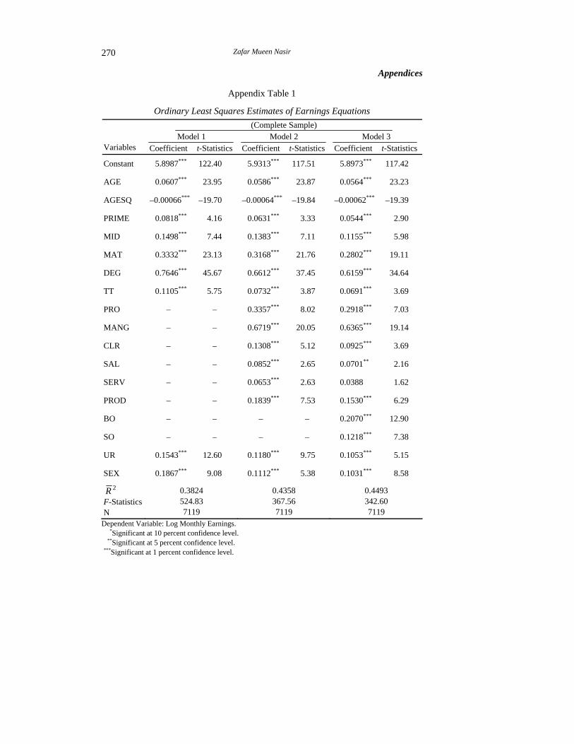
Ordinary Least Squares Estimates of Earnings Equations (Complete Sample)
Model 1 Model 2 Model 3 Variables Coefficient t-Statistics Coefficient t-Statistics Coefficient t-Statistics
Constant 5.8987*** 122.40 5.9313*** 117.51 5.8973*** 117.42
AGE 0.0607*** 23.95 0.0586*** 23.87 0.0564*** 23.23
AGESQ –0.00066*** –19.70 –0.00064*** –19.84 –0.00062*** –19.39
PRIME 0.0818*** 4.16 0.0631*** 3.33 0.0544*** 2.90
MID 0.1498*** 7.44 0.1383*** 7.11 0.1155*** 5.98
MAT 0.3332*** 23.13 0.3168*** 21.76 0.2802*** 19.11
DEG 0.7646*** 45.67 0.6612*** 37.45 0.6159*** 34.64
TT 0.1105*** 5.75 0.0732*** 3.87 0.0691*** 3.69
PRO – – 0.3357*** 8.02 0.2918*** 7.03
MANG – – 0.6719*** 20.05 0.6365*** 19.14
CLR – – 0.1308*** 5.12 0.0925*** 3.69
SAL – – 0.0852*** 2.65 0.0701** 2.16
SERV – – 0.0653*** 2.63 0.0388 1.62
PROD – – 0.1839*** 7.53 0.1530*** 6.29
BO – – – – 0.2070*** 12.90
SO – – – – 0.1218*** 7.38
UR 0.1543*** 12.60 0.1180*** 9.75 0.1053*** 5.15
SEX 0.1867*** 9.08 0.1112*** 5.38 0.1031*** 8.58 2R
F-Statistics N
0.3824 524.83 7119
0.4358 367.56 7119
0.4493 342.60 7119
Dependent Variable: Log Monthly Earnings. *Significant at 10 percent confidence level. **Significant at 5 percent confidence level. ***Significant at 1 percent confidence level.
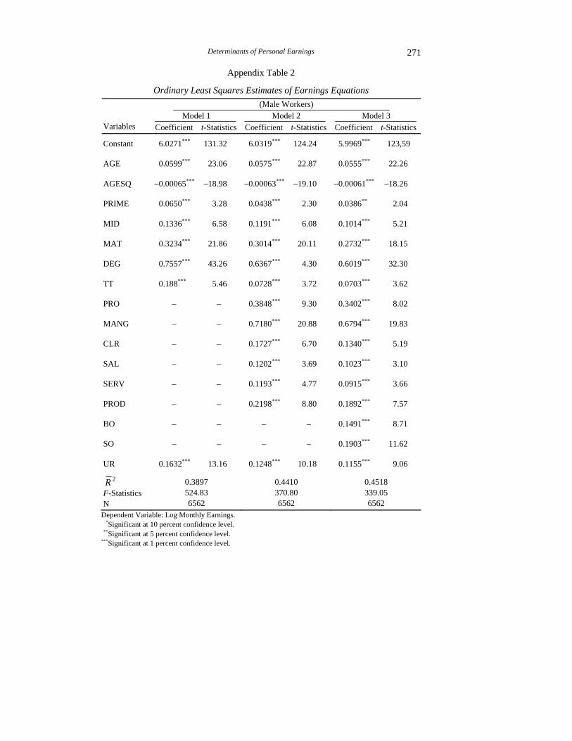
Determinants of Personal Earnings 271
Appendix Table 2
Ordinary Least Squares Estimates of Earnings Equations (Male Workers)
Model 1 Model 2 Model 3 Variables Coefficient t-Statistics Coefficient t-Statistics Coefficient t-Statistics
Constant 6.0271*** 131.32 6.0319*** 124.24 5.9969*** 123,59
AGE 0.0599*** 23.06 0.0575*** 22.87 0.0555*** 22.26
AGESQ –0.00065*** –18.98 –0.00063*** –19.10 –0.00061*** –18.26
PRIME 0.0650*** 3.28 0.0438*** 2.30 0.0386** 2.04
MID 0.1336*** 6.58 0.1191*** 6.08 0.1014*** 5.21
MAT 0.3234*** 21.86 0.3014*** 20.11 0.2732*** 18.15
DEG 0.7557*** 43.26 0.6367*** 4.30 0.6019*** 32.30
TT 0.188*** 5.46 0.0728*** 3.72 0.0703*** 3.62
PRO – – 0.3848*** 9.30 0.3402*** 8.02
MANG – – 0.7180*** 20.88 0.6794*** 19.83
CLR – – 0.1727*** 6.70 0.1340*** 5.19
SAL – – 0.1202*** 3.69 0.1023*** 3.10
SERV – – 0.1193*** 4.77 0.0915*** 3.66
PROD – – 0.2198*** 8.80 0.1892*** 7.57
BO – – – – 0.1491*** 8.71
SO – – – – 0.1903*** 11.62
UR 0.1632*** 13.16 0.1248*** 10.18 0.1155*** 9.06
2R F-Statistics N
0.3897 524.83 6562
0.4410 370.80 6562
0.4518 339.05 6562
Dependent Variable: Log Monthly Earnings. *Significant at 10 percent confidence level. **Significant at 5 percent confidence level. ***Significant at 1 percent confidence level.
Zafar Mueen Nasir 272
Appendix Table 3
Ordinary Least Squares Estimates of Earnings Equations (Female Workers)
Model 1 Model 2 Model 3 Variables Coefficient t-Statistics Coefficient t-Statistics Coefficient t-Statistics Constant 5.5828*** 29.21 5.7621*** 32.34 5.7621*** 32.34 AGE 0.0780*** 7.27 0.0684*** 7.56 0.0684*** 7.56 AGESQ –0.00086*** –5.88 –0.00077*** –6.30 –0.00077*** –6.30 PRIME 0.1047*** 4.04 0.0850** 2.45 0.0623** 2.45 MID 0.1877*** 5.58 0.1694** 2.31 0.1469** 2.31 MAT 0.2912*** 19.23 0.2729*** 2.86 0.2529*** 2.86 DEG 0.3835*** 27.87 0.3502*** 4.78 0.3429*** 4.78 TT 0.0925 1.15 0.0911 1.11 0.803 1.06 PRO – – 0.4338*** 6.53 0.4213*** 6.28 MANG – – 0.9439*** 7.75 0.9439*** 7.48 CLERC – – 0.0614 0.64 0.0512 0.61 SALE – – 0.2523 1.21 0.2468 1.17 SERV – – -0.0913 –1.06 –0.0925 –1.13 PROD – – 0.1271** 2.14 0.1098** 2.05 BO – – – – 0.3446*** 5.48 SO – – – – 0.1130*** 1.76 UR –0.0307*** –0.98 –0.0337 –0.94 –0.0357 –0.76
2R F-Statistics N
0.3610 53.84 555
0.4180 34.54 555
0.4530 34.16 555
Dependent Variable: Log Monthly Earnings. *Significant at 10 percent confidence level. **Significant at 5 percent confidence level. ***Significant at 1 percent confidence level.
Appendix Table 4
Maximum Likelihood Estimates of Probit Equations Complete Sample Male Workers Explanatory
Variables Coefficients t-Statistics Coefficient t-Statistics Constant –2.2133*** –13.68 –2.3049*** –13.85 AGE 0.0350*** 3.72 0.0532*** 5.32 AGESQ –0.00059*** 5.36 –0.00071*** –5.92 PRIM 0.0219*** 3.98 0.4126*** 12.10 MID 02532*** 4.72 1.0995*** 49.75 MAT 0.5266*** 7.92 1.6767*** 36.69 DEG 0.6735*** 18.30 1.8597*** 34.19 TT 0.0372*** 6.10 0.1495*** 7.05 UR 0.0920** 1.99 0.1529*** 16.56 MSP 0.0293** 8.61 0.0265*** 3.15 DRATIO 0.0354 1.68 0.0461 0.92 N 26134 24422
Dependent Variable : WPART. *Significant at 10 percent confidence level. **Significant at 5 percent confidence level. ***Significant at 1 percent confidence level.
Determinants of Personal Earnings 273
REFERENCES
Afzal, Mohammad, and Zafar Mueen Nasir (1987) Is Female Labour Force Participation Really Low and Declining in Pakistan? A Look at Alternative Data Sources. The Pakistan Development Review 26:4 699–707.
Ahmed, Ather M., and Ismail Sirageldin (1994) Internal Migration, Earnings, and the Importance of Self-selection. The Pakistan Development Review 33:3 211–227.
Ashraf, Javed, and Birjees Ashraf (1993) An Analysis of the Male-Female Earnings Differential in Pakistan. The Pakistan Development Review 32:4 895–904.
Becker, Gary S. (1964) Human Capital. New York: National Bureau of Economic Research.
Bowles, Samual (1985) The Production Process in a Competitive Economy: Walrasian, Neo-Hobbesian and Marxian Models. American Economic Review 75: 16–36.
Bulow, Jeremy I., and Lawrence H. Summers (1986) A Theory of Dual Labour Markets with Application to Industrial Policy, Discrimination, and Keynesian Unemployment. Journal of Labour Economics 4: 376–414.
Chaudhry, M. Ghaffar, and Zubeda Khan (1987) Female Labour Force Participation Rates in Rural Pakistan: Some Fundamental Explanations and Policy Implica-tions. The Pakistan Development Review 26:4 687–696.
Dickens, William T., and Lawrence F. Katz (1987) Inter-Industry Wage Differences and Industry Characteristics. In Kevin Lang and Jonathan S. Leonard (eds) Unemployment and the Structure of Labour Markets. New York: Basil Blackwell. 46–89.
Ghayur, Sabur (1993) The Informal Sector of Pakistan: Problems and Policies. Friedrich-Ebert-Stiftung, Islamabad. (The Informal Sector Study No. 3).
Gintis, Herbert (1976) The Nature of the Labour Exchange and the Theory of Capitalist Production. Review of Radical Political Economy 8: 36–54.
Guisinger, S. E., J. W. Henderson, and G. W. Scully (1984) Earnings, Rates of Return to Education, and Earnings Distribution in Pakistan. Economics of Education Review 3:4.
Gujarati, Damodar N. (1988) Basic Econometrics. New York: McGraw Hill. Hamdani, Khalil A. (1977) Education and the Income Differential: An Estimation
For Rawalpindi City. The Pakistan Development Review 26:2 144–164. Haque, Nadeem Ul (1977) Economic Analysis of Personal Earnings in Rawalpindi
City. The Pakistan Development Review 26:4 687–696. Harrison, Bennett, Chirs Tilly, and Barry Bluestone (1986) Wage Inequality Takes a
Great U-turn. Challenge 29: 1 26-32. Heckman, J. (1979) Sample Selection Bias as a Specification Error. Econometrica
47:1.
Zafar Mueen Nasir 274
Juster, F. Thomas, and Frank P. Stafford (1991) The Allocation of Time: Empirical Findings, Behavioural Models and Problems of Measurements. Journal of Economic Literature 29: 471–522.
Karoly, Lynn A. (1992) Changes in the Distribution of Individual Earnings in the United States: 1967-1986. The Review of Economics and Statistics 74:1 107–115.
Khan, Shahrukh Rafi, and Mohammad Irfan (1985) Rate of Returns to Education and the Determinants of Earnings in Pakistan. The Pakistan Development Review 24:3&4 471–680.
Kozel, Valerie, and Harold Alderman (1990) Factors Determining Work Participation and Labour Supply Decisions in Pakistan’s Urban Areas. The Pakistan Development Review 29:1 1–18.
Krueger, Allen B., and Lawrence H. Summers (1988) Efficiency Wages and the Inter-industry Wage Structure. Econometrica 56: 259–293.
Lawrence, Robert Z. (1984) Sectoral Shifts and the Size of the Middle Class. The Brookings Review Fall: 3–11.
Mincer, Jacob (1974) Schooling, Experience and Earnings. New York: National Bureau of Economic Research.
Rebitzer, James (1993) Radical Political Economy and the Economics of Labour Markets. Journal of Economic Literature 31: 1394–1434.
Rebitzer, James, and Michael Robinson (1991) Employer Size and Dual Labour Markets. Review of Economics and Statistics 73: 710–715.
Roemer, John E. (1979) Divide and Conquer: Micro-foundations of a Marxian Theory of Wage Determination. Bell Journal of Economics 10: 695–705.
Shabbir, Tayyeb (1992) Sheepskin Effects in the Returns to Education in a Developing Country. The Pakistan Development Review 30: 1–19.
Shabbir, Tayyeb (1994) Mincerian Earnings Function for Pakistan. The Pakistan Development Review 33:4 1–18.
Shabbir, Tayyeb and Alia H. Khan (1991) Mincerian Earnings Functions for Pakistan: A Regional Analysis. Pakistan Economic and Social Review 24: 99–111.
Thurow, Lester (1987) A Surge in Inequality. Scientific American 256:5 30–37.


![Determinants of Personal Earnings in Pakistan: Findings ... · Irfan (1985); Ashraf and Ashraf (1993); Ahmad and Sirageldin (1994) and others]. But very few have focused on the determinants](https://static.fdocuments.in/doc/165x107/5b35149e7f8b9a330e8cd327/determinants-of-personal-earnings-in-pakistan-findings-irfan-1985-ashraf.jpg)