DETERMINANTS OF INFLATION IN PAKISTAN: AN … · DETERMINANTS OF INFLATION IN PAKISTAN: AN...
12
Australian Journal of Business and Management Research Vol.1 No.5 [71-82] | August-2011 71 DETERMINANTS OF INFLATION IN PAKISTAN: AN ECONOMETRIC ANALYSIS USING JOHANSEN CO-INTEGRATION APPROACH Mr. Furrukh Bashir (Corresponding Author) Ph.D Scholar, Department of Economics, University of the Punjab, Lahore, Pakistan. Email: [email protected] Mr. Shahbaz Nawaz Part time teacher, Masters in Statistics, Bahauddin Zakariya University, Multan, Pakistan. Email: [email protected] Ms. Kalsoom Yasin M.Phil Scholar, Department of Statistics, Bahauddin Zakariya University, Multan, Pakistan Email: [email protected] Mr. Usman Khursheed Part time teacher, Masters in Statistics, Bahauddin Zakariya University, Multan, Pakistan. Email: [email protected] Mr. Jahanzeb Khan Masters in Public Administration Quaid – e – Azam University, Islamabad, Pakistan. Email: [email protected] Mr. Muhammad Junaid Qureshi Masters in Economics, Bahauddin Zakariya University, Multan, Pakistan. Email: [email protected] ABSTRACT Inflation is regarded as regressive taxation against the poor. The most visible impact of inflation in recent times is its effect on real output, relative prices, taxes and interest rates. The study focuses to examine demand side and supply side determinants of inflation in Pakistan on economic and econometric criterion and also to investigate causal relationships among some macroeconomic variables. For that purpose, study has undertaken time series data for the period from 1972 to 2010. Long run and short run estimates have been investigated using Johansen Co-integration and Vector Error Correction approached. Causal relationships have been observed using Granger causality test. Data on macroeconomic variables have been selected from Handbook on Statistics of Pakistan 2010. The findings of the study reveal that in the long run consumer price index has found to be positively influenced by money supply, gross domestic product, imports and government expenditures on the other side government revenue is reducing overall price level in Pakistan. Long run elasticities of Price level with respect to money supply, gross domestic product, government expenditures, government revenue and imports are 0.61, 0.73, 0.32, -1.37 and 0.41 respectively. In the short run, last year consumer price index and two years before government revenue are directly involved in enhancing consumer price index of current year. Improvement in gross domestic product and government expenditures is necessary but it is suggested that there should be optimal level for all of them so that price level should be stable. Keywords: Consumer price index, Government expenditures, gross domestic product, Johansen Co-integration technique, Money supply, Long run elasticities. I. INTRODUCTION Inflation means continuous rise in general price level of the economy. Inflation is process in which the price index is rising and money is losing its value. The issue of inflation takes primary importance in Pakistan as the rising inflation has far reaching economic and social implications. From an economic and business perspective,
Transcript of DETERMINANTS OF INFLATION IN PAKISTAN: AN … · DETERMINANTS OF INFLATION IN PAKISTAN: AN...

Australian Journal of Business and Management Research Vol.1 No.5 [71-82] | August-2011
71
DETERMINANTS OF INFLATION IN PAKISTAN: AN ECONOMETRIC
ANALYSIS USING JOHANSEN CO-INTEGRATION APPROACH
Mr. Furrukh Bashir (Corresponding Author)
Ph.D Scholar, Department of Economics,
University of the Punjab, Lahore, Pakistan.
Email: [email protected]
Mr. Shahbaz Nawaz
Part time teacher, Masters in Statistics,
Bahauddin Zakariya University, Multan, Pakistan.
Email: [email protected]
Ms. Kalsoom Yasin
M.Phil Scholar, Department of Statistics,
Bahauddin Zakariya University, Multan, Pakistan
Email: [email protected]
Mr. Usman Khursheed
Part time teacher, Masters in Statistics,
Bahauddin Zakariya University, Multan, Pakistan.
Email: [email protected]
Mr. Jahanzeb Khan
Masters in Public Administration
Quaid – e – Azam University, Islamabad, Pakistan.
Email: [email protected]
Mr. Muhammad Junaid Qureshi
Masters in Economics,
Bahauddin Zakariya University, Multan, Pakistan.
Email: [email protected]
ABSTRACT
Inflation is regarded as regressive taxation against the poor. The most visible impact of inflation in recent times
is its effect on real output, relative prices, taxes and interest rates. The study focuses to examine demand side
and supply side determinants of inflation in Pakistan on economic and econometric criterion and also to
investigate causal relationships among some macroeconomic variables. For that purpose, study has undertaken
time series data for the period from 1972 to 2010. Long run and short run estimates have been investigated
using Johansen Co-integration and Vector Error Correction approached. Causal relationships have been
observed using Granger causality test. Data on macroeconomic variables have been selected from Handbook on
Statistics of Pakistan 2010. The findings of the study reveal that in the long run consumer price index has found
to be positively influenced by money supply, gross domestic product, imports and government expenditures on
the other side government revenue is reducing overall price level in Pakistan. Long run elasticities of Price level
with respect to money supply, gross domestic product, government expenditures, government revenue and
imports are 0.61, 0.73, 0.32, -1.37 and 0.41 respectively. In the short run, last year consumer price index and
two years before government revenue are directly involved in enhancing consumer price index of current year.
Improvement in gross domestic product and government expenditures is necessary but it is suggested that there
should be optimal level for all of them so that price level should be stable.
Keywords: Consumer price index, Government expenditures, gross domestic product, Johansen Co-integration
technique, Money supply, Long run elasticities.
I. INTRODUCTION
Inflation means continuous rise in general price level of the economy. Inflation is process in which the price
index is rising and money is losing its value. The issue of inflation takes primary importance in Pakistan as the
rising inflation has far reaching economic and social implications. From an economic and business perspective,

Australian Journal of Business and Management Research Vol.1 No.5 [71-82] | August-2011
72
the inflation rate directly relates to gross domestic product, money supply, exports, prices of imports, exchange
rate, interest rate, fiscal deficit, government expenditure, tax revenue etc.
The major problems faced by the society arise due to higher inflation. Due to higher price level, the people need
more money to make day to day transactions and every consumer has to carry more money with them as value
of money declines. Inflation discourages saving and promotes consumption. The effect of inflation severity is
more social than economic due to the erosion of the real value of money the real value of money. The recent
inflationary environment in the country may be blamed to some extent for lower deposit growth and lower
savings. Historically, Pakistan is accustomed to lower inflation and thus has less tolerance towards higher
double digit inflation. In this backdrop persistence of high double digit inflation for third year in a row has
become intolerable and the government is pursuing combination of several policy measures such as the control
of the budget deficit through appropriate fiscal and monetary policies, the improvement of agricultural
productivity, the fostering of investment to stimulate output and the constant vigilance on the market situation to
ensure the adequate availability of consumer goods to the common man at a reasonable price to bring inflation
down to a tolerable and sustainable level.
The year 2010-11 is the most eventful year for the world inflation. The inflation poses serious threat to
macroeconomic stability around the world. More worrying thing is that the recent spike in inflation is coming
more from food inflation which is detrimental for poverty situation, According to ADB study, a 10 percent rise
in food inflation is likely to deteriorate poverty situation by 2.7 percentage points. Inflation may also result from
either increase in aggregate demand or a decrease in aggregate supply, these two sources effect price level of an
economy. An inflation resulting from increase in aggregate demand is called demand pull inflation. Demand
pull inflation arises due to many factors like money supply, government expenditures, exports or gross domestic
product etc. Cost push inflation may be defined as the increase in general price level resulting from increase in
cost of production. The main sources of cost push inflation may be decrease in aggregate supply that may be due
to cost of production, increasing wages, higher imports, rising taxes, budget deficit or fiscal deficit.
The present study aims at investigating both demand and supply side determinants of inflation on the basis of
statistical criterion as well as on economic criterion and also to trace out causal effects of some macroeconomic
variables on inflation of Pakistan. The study is organized as follows: Apart from introduction in section one,
some empirical studies are reviewed in section second, data sources and econometric model are discussed in
section third, fourth section deals with appropriate methodology, in fifth sections, results are discussed on
economic and econometric criterion, and finally sixth section concludes the whole research.
II. REVIEW OF SOME EMPIRICAL STUDIES
Study of determining the factors affecting inflation or consumer price index has been conducted by many
macroeconomic economists nationally as well as internationally. These all are different from each other either
from country to country, sample size, time period or from selection of variables. In this section, few of them are
comprehensively summarized as below;
Lim and Papi (1997) have shed light on the determinants of inflation in Turkey. In this study, they have adopted
time series data from 1970 to 1995. The authors have applied Johansen Co integration technique to find out
results. The analysis concludes that money, wages, prices of exports and prices of imports have positive
influence on domestic price level where as exchange rate exerts inverse effect on the domestic price level in
Turkey.
Kuijs (1998) has analyzed the determinants of three variables; the price level, exchange rate and output. In this
study, the author uses time series data. Moreover vector autoregressive model has been applies to investigate the
relationships. The study suggests that first lag of prices, 3rd
lag of prices, 1st lag of excess money supply and 1
st
lag of output gap are directly related to price level where as 2nd
lag of prices, 4th
lag of prices and output gap are
indirectly linked with price level in Nigeria.
Liu and Adedeji (2000) have established a framework for analyzing the major determinants of inflation in the
Islamic Republic of Iran. Time series data has been chosen from 1989 to 1999 for this study. The authors have
applied Johansen co-integration test and vector error correction model to examine the results. The analysis has
found that lag value of money supply, monetary growth, four years previous expected rate of inflation are
positively contributed towards inflation while two years previous value of exchange premium is negatively
correlated with inflation.

Australian Journal of Business and Management Research Vol.1 No.5 [71-82] | August-2011
73
Laryea and Sumaila (2001) have examined the major determinants of inflation in Tanzania. For this analysis,
they have used the time series data from 1992 to 1998 on quarterly basis. Ordinary least square method has been
applied to have estimates. The analysis demonstrates that money supply and exchange rate have positive
impression on consumer price index while gross domestic product has negative impact on consumer price index
of Tanzania.
Khan et al. (2007) have found the most significant explanatory factors for recent inflation trends in Pakistan.
Time series data from 1972 to 2005 has been used in the study. The authors have employed ordinary least
square method to estimate results. The analysis concludes that government sector borrowing, real demand,
private sector borrowing, import prices, exchange rate, government taxes, previous year consumer price index
and wheat support prices are found to have direct contribution in consumer price index of Pakistan.
Abdullah and Khalim (2009) have explored the main determinants of food price inflation in Pakistan. For that
purpose, they have used time series data for the period from 1972 to 2008. Johansen co-integration technique
has been employed to estimate long run results. The analysis illustrates that money supply; per capita GDP,
agriculture support price, food exports and food imports are direct associated with food inflation in Pakistan.
Mosayed and Mohammad (2009) have traced out the major determinants of inflation in Iran. They have used the
time series data from 1971 to 2006 in their analysis. The study uses Autoregressive and distributed lag model to
discover the long run estimates. The study probes that money supply, exchange rate, gross domestic product,
change in domestic prices and foreign prices are presenting the effect of Iran or Iraq war on Iran’s economy and
all are positively contributing to the domestic prices in Iran.
Khan and Gill (2010) have focused on the determinants of inflation in Pakistan using different price indicators
i.e. CPI, WPI, SPI and GDP Deflator. They have adopted time series data from 1971 to 2005 for the analysis.
Ordinary least square method has been employed for the estimation of values of coefficients. The explanatory
variables that are budget deficit, exchange rate, wheat support price, Imports, Support price of sugarcane and
cotton and money supply are found to be directly affecting all the price indicators while interest rate is indirectly
related to all the explained variables in Pakistan.
Abidemi and Malik (2010) have critically analyzed the dynamic and simultaneous inter relationship between
inflation and its determinants in Nigeria. Johansen co-integration technique and error correction model are used
to analyze determinants of inflation for the time series data for the period from 1970 to 2007. The findings
reveal that growth rate of GDP, money supply, Imports, 1st lag of inflation and interest rate give positive
impression on inflation rate. While other explanatory variables such as fiscal deficit and exchange rate are
indirectly associated to inflation.
Olatunji et al. (2010) have examined the recent factors which are affecting inflation in Nigeria. Time series data
has been selected for this particular study. In this paper they have applied Johansen technique to formulate the
results. The study reveals that the previous year total imports, previous year consumer price index for food,
previous year government expenditure, and previous year exchange rate have negative influence on inflation
rate. On the other side, previous year exports, previous year agricultural output, previous year interest rate and
crude oil exports have negative impact on the rate of inflation in Nigeria.
III. MODEL BUILDING, VARIABLES AND DATA SOURCES
The current study focuses on demand and supply side determinants of inflation in Pakistan and to see causal
relationships of some macroeconomic variables with inflation. For that purpose, we have included both the
factors (demand side and supply side) as given in following equation form;
iiiiiiii LGRLGELXLMLGDPLBMLCPI 654321
Relationships (+) (+) (+) (–) (+) (–)
Dependent Variable:
LCPI = Log of Consumer Price Index based on 2000 prices
Explanatory Variables:
LBM = Log of Broad Money
LGDP = Log of Gross Domestic Product
LM = Log of Imports of Goods and Services

Australian Journal of Business and Management Research Vol.1 No.5 [71-82] | August-2011
74
LX = Log of Exports of Goods and Services
LGE = Log of Government Expenditures
LGR = Log of Government Revenue
= Intercept
’s = Slope Coefficients
= Error term
The contemporary examination uses time series data for the period from 1972 to 2010. Log – log model has
been employed to have the elasticities of price with respect to money supply, gross domestic product, exports,
imports, government expenditures and government revenue. All the data series are taken in current million
rupees. The authors have used Handbook of statistics on Pakistan Economy 2010 as data source published by
government of Pakistan.
IV. METHODOLOGICAL DISCUSSION
Trended time series can potentially create major problems in empirical econometrics due to spurious
regressions. Most macroeconomic variables are trended and therefore the spurious regression problem is highly
likely to be present in most macro econometric models. One way of resolving this is to take difference of the
series successively until stationarity is achieved and then use stationary series for regression analysis. However,
this solution is not ideal. Applying first differences of the variables leads to the loss of long run properties, since
the models in differences have no long run solution. The basic idea is that if there are economic time series that
are integrated and of the same order (they are non stationary), which we know are related (mainly through a
theoretical framework), then trying to check whether we can find a way to combine them together into a single
series which is itself non stationary. If this is possible, then the series that exhibits this property is called co-
integrated.
Elliot, Rothenberg, and Stock Point Optimal Unit Root Test (ERS)
The ERS point optimal test is based on the quasi – differencing regression defined follows;
)()(ˆ)|()|( aaaxdayd ttt
Where xt contains either a constant, or a constant and trend, and let )(ˆ a be the OLS estimates from
regression. Define the residuals as )(ˆ)|()|()( aaxdayda ttt , and let SSR( a ) = )(ˆ 2 at be the
sum of squared residuals function. The ERS (feasible) point optimal test statistic of the null that 1 against
the alternative that a , is then defined as;
PT = (SSR ( a ) - a SSR (1)) / f0
Where, f0 is an estimator of the residual spectrum at frequency zero. To compute the ERS test, you must specify
the set of exogenous regressors xt and a method for estimating f0. Critical values for the ERS test statistic are
computed by interpolating the simulation results provided by ERS. The Null hypothesis for ERS unit test is that
variable has a unit root.
Information Criteria (Lag length Selection)
The information criteria are often used as a guide in model selection. The Kullback – Leibler quantity of
information contained in a model is the distance from the true model and is measured by the log likelihood
function. The notion of an information criterion is to provide a measure of information that strikes a balance
between this measure of goodness of fit and parsimonious specification of the model. The various information
criteria differ in how to strike this balance.
The basic information criteria are given by;
Akaike info criterion (AIC) = - 2 ( l / T ) + 2 ( k / T)
Schwarz Criterion (SC) = - 2 ( l / T ) + k log ( T) / T
Hannan – Quinn criterion (HQ) = - 2 ( l / T ) + 2 k log ( log ( T)) / T

Australian Journal of Business and Management Research Vol.1 No.5 [71-82] | August-2011
75
Johansen Co-integration Technique
Johansen (1988) and Johansen and Juselius (1990) have given new technique for co-integration for long run as
well as short run relationships for multivariate equation as explained below. Let’s assume that we have three
variables, Yt, Xt and Wt which can all be endogenous, i.e. we have that (using matrix notation for Zt = [Tt, Xt,
Wt]).
Zt = A1 Zt-1 + A2 Zt-2 + ................ + Ak Zt-k + ut
It can be reformulated in a vector error correction model (VECM) as follows;
∆Zt = r1 ∆Zt-1 + r2 ∆Zt-2 + ................ + rk-1 ∆Zt-k + ∏ Zt-1 + ut
Where ri = (I – A1 – A2 – ….. – Ak) (I = 1, 2, ….., k-1) and ∏ = – ( I – A1 – A2 – ….. – Ak). Here we need to
carefully examine the 3 Χ 3 ∏ matrix (The ∏ matrix is 3 Χ 3 due to the fact that we assume three variables in Zt
= [Tt, Xt, Wt]). The ∏ matrix contains information regarding the long run relationship. In fact ∏ = a where
a will include the speed of adjustment to equilibrium coefficients while will be the long run matrix of
coefficients
Therefore the Zt-1 term is equivalent to the error correction term (Yt-1 – β0 – β1 Xt-1) in the single equation
case, except that now Zt-1 contains up to (n – 1) vectors in a multivariate framework.
For simplicity we assume that k = 1, so that we have only two lagged terms and the model is then the following:
t
t
t
t
t
t
t
t
t
t
e
W
X
Y
W
X
Y
r
W
X
Y
1
1
1
1
1
1
1
Or t
t
t
t
t
t
t
t
t
t
e
W
X
Y
aa
aa
aa
W
X
Y
r
W
X
Y
1
1
1
32
31
22
21
12
11
2331
2221
1211
1
1
1
1
Let us now analyze only the error correction part of the first equation (i.e. for ∆Yt on the left hand side) which
gives;
1
1
1
111-t1 ([ Z
t
t
t
W
X
Y
aaaaaa
Where, ∏1 is the first row of the ∏ matrix. The above equation can be rewritten as;
1212131311111-t1 () ( Z tttttt WXYaWXYa
Which shows clearly the co-integrating vectors with their respective speed of adjustment terms 11a and a .
Johansen (1988) and Johansen and Juselius (1990) have proposed few steps for reliable results discussed below.
1. For the application of Johansen Co-integration approach, all time series variables involving in the study
should be integrated of order one [I(1)].
2. At second step, lag length would be chosen using VAR model on the basis of minimum values of Final
Predication Error (FPE), Akaike Information Criterion (AIC), and Hannan and Quinn information criterion
(HQ).
3. At third step, appropriate model regarding the deterministic components in the multivariate system are to be
opted.
4. Johansen (1988) and Johansen and Juselius (1990) examine two methods for determining the number of co-
integrating relations and both involve estimation of the matrix ∏. Maximal eigenvalue statistics and trace
statistic are utilized in 4th
step for no of co-integrating relationships and also for the values of coefficients and
standard errors regarding econometric model.
Vector Error Correction Mode (VECM)
A vector error correction model is a restricted vector autoregressive (VAR) designed for use with non stationary
series that are known to be co-integrated. It may be tested for co-integration using an estimated VAR object.

Australian Journal of Business and Management Research Vol.1 No.5 [71-82] | August-2011
76
The VECM has co-integration relations built into the specification so that it restricts the long run behavior of the
endogenous variables to converge to their co-integrating relationships while allowing for short run adjustment
dynamics. The co-integration term is known as the error correction term (speed of adjustment) since the
deviation from long run equilibrium is corrected gradually through a series of partial short run adjustments. The
Short run equation is given below;
q
j
tt
q
j
q
j
q
j
q
j
q
j
q
j
ECMLGRaLGEaLXa
LMaLBMaLGDPaLCPIaa
LCPI
jtjtjt
jtjtjtjt
0
111
0
7
0
65
0 0
43
0
2
1
10
Where, ∆ is difference operator, q is chosen lag length, a’s are parameters, is error correction term or speed
of adjustment term (calculated from long run results) and is error term.
Granger Causality Test
The granger causality test for the case of two variables Yt and Xt, involves following steps as the estimation of
the following VAR model;
1
11
1 eYrXbaYq
j
jti
p
i
itit
2
11
2 eXdYcaXq
j
jtj
p
i
itit
Where, it is assumed that both e1 and e2 are uncorrelated white noise error terms.
V. DISCUSSION ON ECONOMETRIC AND ECONOMIC CRITERION
Examination of Unit root test
Johansen Co-integration technique requires confirming the order of integration of all the variables used in the
study. Table 1 reports the results of ERS unit root test and corroborate that all the variables are integrated at
order one.
Table 1: ERS Unit Root Test
Variables Tests for
Unit Root in
Include in
Test Equation
P - Statistics
Result ERS Test
Statistics
Critical
Value
LCPI Level
Intercept 511.64 1.87*
I(1) Trend and Intercept 985.99 4.22*
1st Difference Intercept 1.8901 2.97**
LBM Level
Intercept 3543.51 1.87*
I(1) Trend and Intercept 7.55 4.22*
1st Difference Intercept 0.81 1.87*
LGDP Level
Intercept 4578.38 1.87*
I(1) Trend and Intercept 47.28 4.22*
1st Difference Intercept 2.15 2.97**
LGE Level
Intercept 1179.49 1.87*
I(1) Trend and Intercept 34.51 4.22*
1st Difference Intercept 3.36 3.91***
LGR Level
Intercept 2680.43 1.87*
I(1) Trend and Intercept 72.72 4.22*
1st Difference Intercept 3.52 3.91***
LM Level
Intercept 239.10 1.87*
I(1) Trend and Intercept 46.00 4.22*
1st Difference Intercept 1.69 1.87*
LX Level
Intercept 81.28 1.87*
I(1) Trend and Intercept 7.28 6.77***
1st Difference Intercept 0.79 1.87*
Note: *, **, *** shows critical values at 1, 5 and 10 percent level of significance

Australian Journal of Business and Management Research Vol.1 No.5 [71-82] | August-2011
77
Lag Length Selection Process
Second step of Johansen Co-integration technique involves the selection of appropriate lag length using proper
information criterions. We have used Final Prediction error, Akaike information criterion and Hannan – Quinn
information criterion in our study and results are reported in table 2. Favorable lag length that is selected in
current analysis is assumed to be 2 at which the values of information criterions are minimum.
Table 2: Lag length Selection
Lag FPE AIC HQ
0 2.61e-11 -4.5056 -4.398
1 6.26e-16 -15.190 -14.331
2 2.87e-16* -16.268* -14.656*
* indicates lag order selected by the criterion calculated using EViews-7
FPE: Final prediction error
AIC: Akaike information criterion
HQ: Hannan-Quinn information criterion
No. of Co-integrated Vectors
At third step, the study has found number of co-integrated equations using trace statistics and maximum
eigenvalue statistics. According to probabilities given in tables 3 and 4, the analysis rejects the null hypothesis
that there is no co-integrated vector (None), there is at most 1 co-integrated vector (At most 1), there is at most 2
co-integrated vectors (At most 2), there is 3 co-integrated vectors (At most 3) and also there is at most 4 co-
integrated vectors (At most 4). It means that there are 5 co-integrated vectors in long run results. It shows high
association between explanatory and dependent variables used in current study.
Table 3: Trace Statistics
Unrestricted Co-integration Rank Test (Trace)
Hypothesized No. of E(s) Eigenvalue Trace Statistic 0.05 Critical Value Prob.**
None * 0.880 238.673 125.615 0.000
At most 1 * 0.799 162.113 95.753 0.000
At most 2 * 0.630 104.176 69.818 0.000
At most 3 * 0.580 68.355 47.856 0.000
At most 4 * 0.554 37.124 29.797 0.006
At most 5 0.182 8.051 15.494 0.459
At most 6 0.021 0.764 3.841 0.382
Table 4: Eigenvalue Statistics
Unrestricted Co-integration Rank Test (Maximum Eigenvalue)
Hypothesized No. of CE(s) Eigenvalue Max-Eigen Stats Critical Value Prob.**
None * 0.880 76.560 46.231 0.000
At most 1 * 0.799 57.937 40.077 0.000
At most 2 * 0.630 35.820 33.876 0.029
At most 3 * 0.580 31.231 27.584 0.016
At most 4 * 0.554 29.072 21.131 0.003
At most 5 0.183 7.287 14.264 0.455
At most 6 0.021 0.764 3.841 0.382

Australian Journal of Business and Management Research Vol.1 No.5 [71-82] | August-2011
78
Johansen Co-integration (Long run Estimates)
The long run estimates of inflation model are reported in table 5. First column is showing the names of
variables, similarly, coefficients, standard errors and t-statistics are displayed in 2nd
, 3rd
and 4th
columns. 5th
column concludes the significant and insignificant relationships of all the variables. The results reveal that
money supply is found to be directly related to the price level in case of Pakistan. The coefficient having
positive sign is significant at 1 percent level of significance suggesting that 1 percent increase in money supply
leads to 0.61 percent increase in consumer price index on the average in the long run. Price elasticity with
respect to broad money or money supply is 0.61. The result is according to macroeconomic phenomenon of
classical economists given in quantity theory of money as increase in money supply leads to higher price levels.
Due to higher money supply, more funds will be available to invest in the economy, investment will be taken
place, more employment will be generated, aggregate demand will increase, and finally there will be increase in
consumer price index. It affects price level through demand side. Our results are consistent with previous
findings of Liu and Adedeji (2000), Mosayed and Mohammad (2009), Kuijs (1998), Lim and Papi (1997),
Laryea and Sumaila (2001), Khan and Gill (2010), and Abdullah and Kalim (2009). As expected, gross
domestic product is inducing consumer price index at 1 percent level of significance implying that consumer
price index will increase by 0.734 percent due to 1 percent increase in gross domestic product on the average in
the long run. The Price elasticity with respect to gross domestic product is 0.734. The rationale may be that
higher income level leads to higher aggregate demand of goods and services and eventually price level will
increase due to higher demand. Gross domestic product influences inflation through demand side. Our findings
are matched with previous findings of Mosayed and Mohammad (2009), and Abdullah and Kalim (2009).
Similarly, government expenditures are also tended to raise consumer price index of Pakistan. This variable is
significant at 5 percent level of significant with positive coefficient value. On the average in the long run, it
proposes 0.322 percent enhancement in consumer price index due to one more percent increase in government
expenditures. Elasticity of Price with respect to government expenditure is 0.322. Government expenditures also
affects through demand side, as due to more expenditure, aggregate demand of goods and services will increase
and it would lead to higher prices overall in the economy. Same relationship has been established by Olatunji et
al. (2010).
With regards to government revenue, it is having inverse effects on consumer price index. The sign of
coefficient is negative and significant at 1 percent level of significance as well. One percent rise in tax collection
would be cause of 1.377 percent lower price level in the long run on the average. Price elasticity with respect to
government revenues is -1.377. It may be interpreted as due to one more percent increase in tax collection of
government, the disposable income will decrease, due to lower income available to purchase goods and services,
demand of goods and services will decline, and it will eventually lead to surplus supply and hence lower
consumer price index. It has influence on inflation through supply side.
In the same manner, the study includes also imports of goods and services; surprisingly it gives positive
impression on consumer price index of Pakistan [Olatunji et al. (2010), Lim and Papi (1997), Khan and Gill
(2010), Abdullah and Kalim (2009)]. If imports of goods and services will be raised by 1 percent, price level
will increase by 0.406 percent on the average in the long run. Price elasticity with respect to imports is 0.406.1
This may be justified as due to more imports of goods and services, income level will decline, due to declined
income, investment will be less as well, production of goods and services will be lesser than as past and hence
there will be reduced amount of supply of goods and services and it will be cause of higher inflation in Pakistan.
Imports are also supply side factor.
Table 5: Johansen Long run Results
Variables Coefficients Standard Errors T-Statistics Conclusion
LBM 0.610* 0.178 3.417 Significant
LGDP 0.734* 0.128 5.720 Significant
LGE 0.322** 0.155 2.077 Significant
LGR - 1.377* 0.265 - 5.184 Significant
LM 0.406* 0.055 7.284 Significant
LX - 0.011 0.045 - 0.241 Insignificant
CONSTANT 5.150 --- --- ---

Australian Journal of Business and Management Research Vol.1 No.5 [71-82] | August-2011
79
Coming towards exports of goods and services, the sign of coefficient of exports reveals that it is cause of
decline in aggregate prices of Pakistan. But the relationship is insignificant due to having t – ratio lesser than 2.
The negative relationship may be defined as due to higher exports of goods and services, the net trade revenue
will increase, due to higher income of economy, more investment will be taken place, more goods and services
will be produced, aggregate supply will be more than aggregate demand and hence it results in lower price level
in overall economy. Negative sign may also be justified by the argument that due to higher exports, domestic
industry will achieve economies of scale, cost of production will reduce and eventually price level will come
down. Exports also effect through demand side. Our results are reconciliated with the findings of Olatunji et al.
(2010).
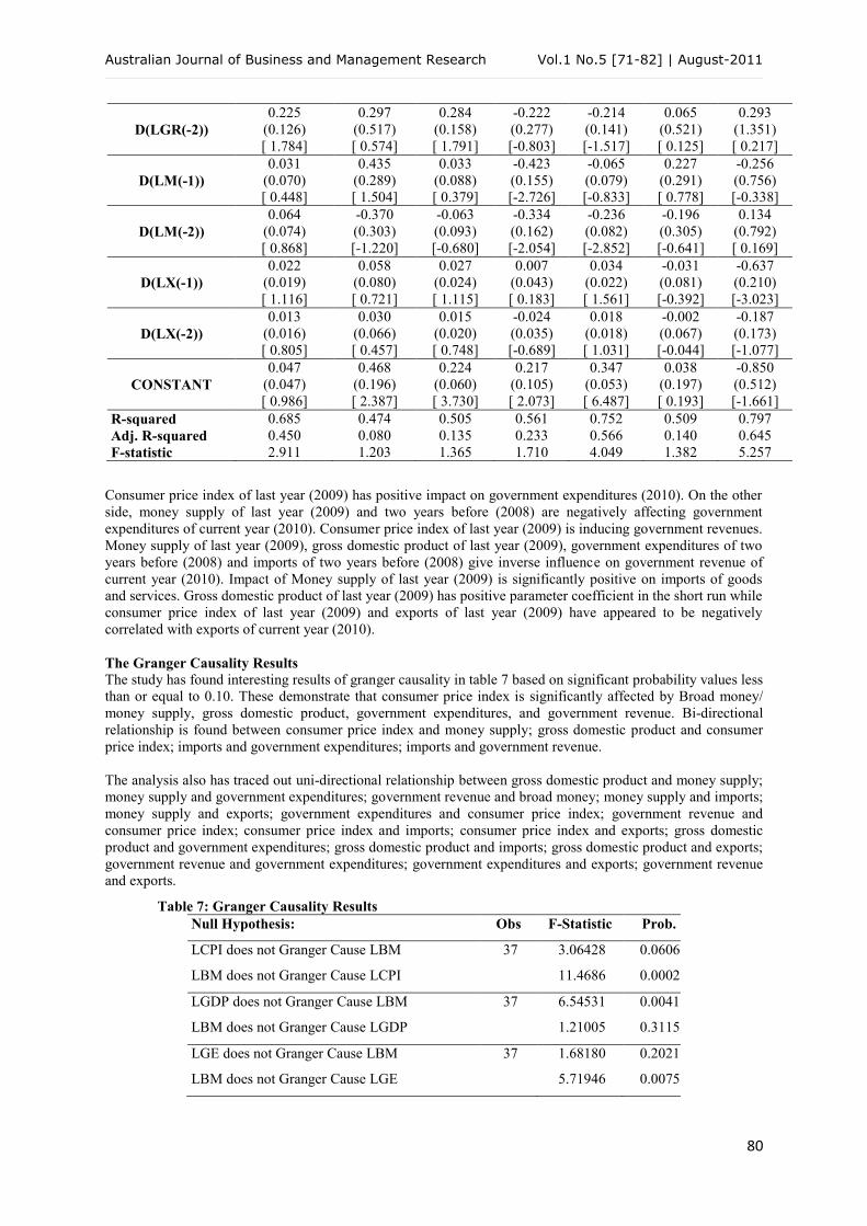
Vector Error Correction Model (Short run Results)
Table 6 discusses the short run results using vector error correction model. Values without brackets are short run
coefficients, values in round brackets are showing standard errors and square brackets are denoting t – statistics.
The most important thing in the short run results is speed of adjustment term. It shows that how much time
would be taken by the economy to reach at long run equilibrium. Negative sign of speed of adjustment term
shows that the economy will converge towards long run equilibrium after taking 3 percent annually adjustments
in the short run however the value of coefficient is statistically insignificant.
Short run results of Vector error correction model (VECM) reveal that consumer price index of last year (2009),
and government revenue of two years before (2008) are found to be positively related with consumer price index
of 2010. Money supply of last year (2009) and two years before (2008) and government expenditure of two
years before (2008) are negatively affecting money supply of current year (2010). Gross domestic product of
current year (2010) is positively affected by Consumer price index of last year (2009) and government revenue
of two years before (2008). While gross domestic product of two years before (2008) is exerting negative
influence on gross domestic product of current year (2010).
Table 6: Vector Error Correction Short run results
Variables D(LCPI) D(LBM) D(LGDP) D(LGE) D(LGR) D(LM) D(LX)
Speed of
Adjustment
-0.037
(0.080)
[ 0.460]
-0.100
(0.329)
[-0.304]
-0.071
(0.100)
[-0.705]
-0.667
(0.176)
[-3.782]
-0.544
(0.089)
[-6.068]
-0.320
(0.331)
[-0.967]
0.220
(0.859)
[ 0.256]
D(LCPI(-1)) 0.492
(0.229)
[ 2.145]
0.732
(0.940)
[ 0.778]
0.620
(0.288)
[ 2.152]
0.917
(0.503)
[ 1.819]
1.066
(0.256)
[ 4.155]
0.357
(0.947)
[ 0.377]
-7.646
(2.455)
[-3.113]
D(LCPI(-2)) 0.0549
(0.250)
[ 0.219]
1.539
(1.026)
[ 1.500]
0.365
(0.314)
[ 1.162]
-0.054
(0.549)
[-0.098]
0.301
(0.279)
[ 1.075]
-0.647
(1.033)
[-0.626]
1.951
(2.678)
[ 0.728]
D(LBM(-1))
-0.064
(0.063)
[-1.018]
-0.611
(0.258)
[-2.367]
-0.105
(0.079)
[-1.329]
-0.063
(0.138)
[-0.455]
-0.167
(0.070)
[-2.376]
0.498
(0.260)
[ 1.913]
0.1030
(0.674)
[ 0.153]
D(LBM(-2))
-0.031
(0.088)
[-0.354]
-0.867
(0.364)
[-2.380]
-0.075
(0.111)
[-0.672]
0.059
(0.195)
[ 0.304]
-0.165
(0.099)
[-1.664]
0.453
(0.366)
[ 1.234]
0.996
(0.950)
[ 1.047]
D(LGDP(-1))
-0.051
(0.210)
[-0.244]
-1.097
(0.863)
[-1.271]
-0.427
(0.264)
[-1.616]
-0.400
(0.462)
[-0.865]
-0.665
(0.235)
[-2.827]
0.228
(0.869)
[ 0.263]
11.281
(2.254)
[ 5.004]
D(LGDP(-2)) -0.405
(0.301)
[-1.346]
-1.065
(1.233)
[-0.863]
-0.851
(0.378)
[-2.252]
0.295
(0.660)
[ 0.446]
-0.436
(0.336)
[-1.296]
-0.388
(1.242)
[-0.312]
-2.599
(3.220)
[-0.807]
D(LGE(-1))
0.040
(0.102)
[ 0.396]
-0.032
(0.420)
[-0.077]
-0.096
(0.128)
[-0.747]
-0.301
(0.225)
[-1.337]
-0.104
(0.114)
[-0.911]
-0.252
(0.423)
[-0.595]
-0.655
(1.098)
[-0.597]
D(LGE(-2))
-0.024
(0.080)
[-0.310]
-0.555
(0.327)
[-1.693]
-0.051
(0.100)
[-0.513]
-0.111
(0.175)
[-0.635]
-0.189
(0.089)
[-2.124]
-0.080
(0.330)
[-0.242]
0.916
(0.855)
[ 1.071]
D(LGR(-1))
0.150
(0.130)
[ 1.153]
0.202
(0.533)
[ 0.378]
0.145
(0.163)
[ 0.889]
0.244
(0.285)
[ 0.854]
-0.135
(0.145)
[-0.933]
0.044
(0.537)
[ 0.082]
0.263
(1.393)
[ 0.189]
Australian Journal of Business and Management Research Vol.1 No.5 [71-82] | August-2011
80
D(LGR(-2))
0.225
(0.126)
[ 1.784]
0.297
(0.517)
[ 0.574]
0.284
(0.158)
[ 1.791]
-0.222
(0.277)
[-0.803]
-0.214
(0.141)
[-1.517]
0.065
(0.521)
[ 0.125]
0.293
(1.351)
[ 0.217]
D(LM(-1))
0.031
(0.070)
[ 0.448]
0.435
(0.289)
[ 1.504]
0.033
(0.088)
[ 0.379]
-0.423
(0.155)
[-2.726]
-0.065
(0.079)
[-0.833]
0.227
(0.291)
[ 0.778]
-0.256
(0.756)
[-0.338]
D(LM(-2))
0.064
(0.074)
[ 0.868]
-0.370
(0.303)
[-1.220]
-0.063
(0.093)
[-0.680]
-0.334
(0.162)
[-2.054]
-0.236
(0.082)
[-2.852]
-0.196
(0.305)
[-0.641]
0.134
(0.792)
[ 0.169]
D(LX(-1))
0.022
(0.019)
[ 1.116]
0.058
(0.080)
[ 0.721]
0.027
(0.024)
[ 1.115]
0.007
(0.043)
[ 0.183]
0.034
(0.022)
[ 1.561]
-0.031
(0.081)
[-0.392]
-0.637
(0.210)
[-3.023]
D(LX(-2))
0.013
(0.016)
[ 0.805]
0.030
(0.066)
[ 0.457]
0.015
(0.020)
[ 0.748]
-0.024
(0.035)
[-0.689]
0.018
(0.018)
[ 1.031]
-0.002
(0.067)
[-0.044]
-0.187
(0.173)
[-1.077]
CONSTANT
0.047
(0.047)
[ 0.986]
0.468
(0.196)
[ 2.387]
0.224
(0.060)
[ 3.730]
0.217
(0.105)
[ 2.073]
0.347
(0.053)
[ 6.487]
0.038
(0.197)
[ 0.193]
-0.850
(0.512)
[-1.661]
R-squared 0.685 0.474 0.505 0.561 0.752 0.509 0.797
Adj. R-squared 0.450 0.080 0.135 0.233 0.566 0.140 0.645
F-statistic 2.911 1.203 1.365 1.710 4.049 1.382 5.257
Consumer price index of last year (2009) has positive impact on government expenditures (2010). On the other
side, money supply of last year (2009) and two years before (2008) are negatively affecting government
expenditures of current year (2010). Consumer price index of last year (2009) is inducing government revenues.
Money supply of last year (2009), gross domestic product of last year (2009), government expenditures of two
years before (2008) and imports of two years before (2008) give inverse influence on government revenue of
current year (2010). Impact of Money supply of last year (2009) is significantly positive on imports of goods
and services. Gross domestic product of last year (2009) has positive parameter coefficient in the short run while
consumer price index of last year (2009) and exports of last year (2009) have appeared to be negatively
correlated with exports of current year (2010).
The Granger Causality Results
The study has found interesting results of granger causality in table 7 based on significant probability values less
than or equal to 0.10. These demonstrate that consumer price index is significantly affected by Broad money/
money supply, gross domestic product, government expenditures, and government revenue. Bi-directional
relationship is found between consumer price index and money supply; gross domestic product and consumer
price index; imports and government expenditures; imports and government revenue.
The analysis also has traced out uni-directional relationship between gross domestic product and money supply;
money supply and government expenditures; government revenue and broad money; money supply and imports;
money supply and exports; government expenditures and consumer price index; government revenue and
consumer price index; consumer price index and imports; consumer price index and exports; gross domestic
product and government expenditures; gross domestic product and imports; gross domestic product and exports;
government revenue and government expenditures; government expenditures and exports; government revenue
and exports.
Table 7: Granger Causality Results
Null Hypothesis: Obs F-Statistic Prob.
LCPI does not Granger Cause LBM 37 3.06428 0.0606
LBM does not Granger Cause LCPI 11.4686 0.0002
LGDP does not Granger Cause LBM 37 6.54531 0.0041
LBM does not Granger Cause LGDP 1.21005 0.3115
LGE does not Granger Cause LBM 37 1.68180 0.2021
LBM does not Granger Cause LGE 5.71946 0.0075

Australian Journal of Business and Management Research Vol.1 No.5 [71-82] | August-2011
81
LGR does not Granger Cause LBM 37 2.56222 0.0929
LBM does not Granger Cause LGR 0.46027 0.6352
LM does not Granger Cause LBM 37 0.41814 0.6618
LBM does not Granger Cause LM 9.07424 0.0008
LX does not Granger Cause LBM 37 0.15490 0.8571
LBM does not Granger Cause LX 10.1452 0.0004
LGDP does not Granger Cause LCPI 37 11.8252 0.0001
LCPI does not Granger Cause LGDP 2.68252 0.0837
LGE does not Granger Cause LCPI 37 9.70499 0.0005
LCPI does not Granger Cause LGE 0.62137 0.5436
LGR does not Granger Cause LCPI 37 9.48111 0.0006
LCPI does not Granger Cause LGR 0.45805 0.6366
LM does not Granger Cause LCPI 37 1.10338 0.3440
LCPI does not Granger Cause LM 2.88252 0.0706
LX does not Granger Cause LCPI 37 0.12975 0.8788
LCPI does not Granger Cause LX 10.0624 0.0004
LGE does not Granger Cause LGDP 37 1.78391 0.1843
LGDP does not Granger Cause LGE 2.62765 0.0878
LGR does not Granger Cause LGDP 37 0.86876 0.4291
LGDP does not Granger Cause LGR 1.71568 0.1960
LM does not Granger Cause LGDP 37 0.81847 0.4501
LGDP does not Granger Cause LM 4.00840 0.0280
LX does not Granger Cause LGDP 37 1.73934 0.1918
LGDP does not Granger Cause LX 14.1929 0.0000
LGR does not Granger Cause LGE 37 4.83499 0.0146
LGE does not Granger Cause LGR 0.69584 0.5060
LM does not Granger Cause LGE 37 2.48045 0.0997
LGE does not Granger Cause LM 3.06621 0.0605
LX does not Granger Cause LGE 37 0.35051 0.7070
LGE does not Granger Cause LX 10.7777 0.0003
LM does not Granger Cause LGR 37 3.07992 0.0598
LGR does not Granger Cause LM 7.01402 0.0030
LX does not Granger Cause LGR 37 0.08244 0.9211
LGR does not Granger Cause LX 11.0065 0.0002
LX does not Granger Cause LM 37 1.09030 0.3483
LM does not Granger Cause LX 2.12092 0.1365
VI. CONCLUDING REMARKS AND POLICY SUGGESTIONS
The study carries out long run as well as short run estimates of some factors influencing consumer price index
(inflation) in Pakistan. The results of the analysis reveal that in the long run money supply, gross domestic
product, government expenditures and imports are contributed in raising consumer price index while consumer
Australian Journal of Business and Management Research Vol.1 No.5 [71-82] | August-2011
82
price index is bound to decrease due to higher government revenues. In the short run, the coefficient of error
correction term is -0.03 suggesting 3 percent annual adjustment towards long run equilibrium. Consumer price
index of last year (2009), consumer price index of two years before (2008) and government revenue of two year
before (2008) have a net positive effect on consumer price index of current year (2010) in the short run.
Long run elasticities of Price level with respect to money supply, gross domestic product, government
expenditures, government revenue and imports are 0.61, 0.73, 0.32, -1.37 and 0.41 respectively. Causality
inferences are quite interesting implying bi-directional as well as uni-directional relationships among few
variables. But money supply, gross domestic product, government expenditures and government revenue are
playing role to have significant effect on consumer price index. At the end, it is suggested that gross domestic
product, government expenditure, and imports should not be as much higher that these all raise the price level
those are not in favor of any economy.
REFERENCES
1. Abdullah, M. and Kalim, R. (2009). Determinants of food price inflation in Pakistan. Paper presented
in the conference of University of Management Sciences, 1 – 21.
2. Abidemi, O. I. and Malik, S. A. A. (2010). Analysis of Inflation and its determinant in Nigeria.
Pakistan Journal of Social Sciences, 7(2), 97 – 100.
3. Akaike, H. (1987), Factor analysis and AIC. Psychometrika, 52(3), 317 – 332.
4. Asteriou, D. (2006). Applied Econometrics A modern approach using Eviews and Microfit. Palgrave
Macmillan.
5. Ekelund, R. B. and Delorme, C. D. (1987). Macroeconomic, 2nd
Edition.
6. Elliott, Graham, Thomas., J. R. and James, H. S. (1996). Efficient tests for an autoregressive unit root.
Econometrica, 64, 813 – 836.
7. Engle, R. F. and Granger, C. W. J. (1987). Co-integration and Error Correction: Representation,
Estimation, and Testing. Econometrica, 55, 251 – 276.
8. Government of Pakistan (2010). Handbook of Statistics on Pakistan Economy. State bank of Pakistan.
9. Johansen, S (1988). Statistical Analysis of Cointegrating Vectors. Journal of Economic Dynamics and
Control, 12, 231-54.
10. Johansen, S. and Juselius, K. (1990). Maximum Likelihood Estimation and Inferences on Cointegration
– with applications to the demand for money. Oxford Bulletin of Economics and Statistics, 52, 169 –
210.
11. Khan, A. A., Bukhari, S. K. H. and Ahmad, Q. M. (2007), Determinants of Recent Inflation in
Pakistan. MPRA paper no. 16254, 1 – 16.
12. Khan, R. E. A. and Gill, A. R. (2010). Determinants of Inflation: A Case of Pakistan (1970 – 2007).
Journal of Economics, 1(1), 45 – 51.
13. Kuijs, L. (1998). Determinants of inflation, exchange rate and output in Nigeria. IMF working paper
no. 160, 1 – 33.
14. Kullback, S. and Leibler, R. A. (1951). On Information and Sufficiency. Annuals of Mathematical
Statistics, 22, 79 – 86.
15. Laryea, S. A. and Sumaila, U. R. (2001). Determinants of Inflation in Tanzania. Chr. Michelsen
Institute Development Studies and Human Rights, WP-12, 1 – 17.
16. Lim, C. H. and Papi, L. (1997). An Econometric Analysis of the determinants of Inflation in Turkey.
IMF Working paper no. 170, 1 – 32.
17. Liu, O. and Adedeji, O. S. (2000). Determinants of Inflation in the Islamic Republic of Iran: A
Macroeconomic analysis. IMF Working paper 127, 1 – 28.
18. Mosayeb, P and Mohammad, R. (2009). Sources of Inflation in Iran: An application of the real
approach. International Journal of Applied Econometrics and Quantitative Studies, 6(1), 61 – 76.
19. Olatunji, G. B. Omotesho, O. A., Ayinde, O. E. and Ayindo, K. (2010). Determinants of Inflation in
Nigeria: A Co-integration approach. Paper presented at the Joint 3rd
African association of agricultural
economists, 1 – 12.