Determinants of Global Palm Oil Demand: A Gravity Approach

Economic Journal of Emerging Markets, 10(2) 2018, 148-164

Econ.J.Emerg.Mark. Available athttp://journal.uii.ac.id/index.php/jep

P ISSN 2086-3128 | E ISSN 2502-180X

Copyright @ 2018 Authors. This is an open-access article distributed under the terms of the Creative Commons Attribution License

(http://creativecommons.org/licences/by-sa/4.0/)

Determinants of Global Palm Oil Demand: A Gravity Approach

Rini Yayuk Priyati *

The University of Western Australia and Universitas Terbuka, IndonesiaCorresponding Author e-mail: [email protected]

Article Info

Article history:

Received : 16 January 2016Accepted : 2 July 2018Published : 1 October 2018

Keywords:

Palm oil, trade, gravity model

JEL Classification:

F14, Q17

Abstract

This paper reviews the determinants of global palm oil trade using the gravitymodel. This model helps to explain how the shift in demand for palm oil has affectedtrade flows among trading partners. We decompose the effects of growth in theregional markets, location, and the reduction in the palm oil price relative to otheredible oils, on palm oil exports. We find that standard variables suggested by thegravity literature, such as the growth of GDP, GDP per capita, and location, areindeed important determinants of palm oil trade. Given the preceding results, we

simulate whether the economic growth of Indonesia☂s trading partners can explainthe growth in palm oil export demand from Indonesia. The simulation results fortop ten Indonesia☂s trading partners suggest that the growth of palm oil imports isa great deal higher than the growth of income for all countries.

Introduction

Palm oil (PO) is a type of vegetable oil derived from oil palm (Elaeis guineensis Jacq.) fresh fruit bunch (FFB).

Oil palm cultivation is found in tropical areas of Africa, South America, and South East (SE) Asia. The history

of oil palm cultivation and trade began in Africa and was associated with the slave trade in the 16th century.

However, the modern development of the PO industry in Africa has lacked behind SE Asia, particularly

Indonesia and Malaysia, the two largest PO producers globally.

The vast growth in global PO demand is undeniable. In fact, PO is one of the fastest growing perennial

crops in the world (Koh & Wilcove, 2008). However, the industrialisation of PO was only prominent after the

1980s. The global PO trade has increased more than five-fold from 1990 to 2015, or from 8.3 million tonnes to

45.1 million tonnes (USDA-FAS, 2016).

However, PO industry development is also one of the most controversial global problems, as it is argued

to be one of the major sources of deforestation, particularly in biodiversity-rich countries like Indonesia and

Malaysia. In 2013, the total area of global oil palm plantation was 18.1 million hectares, increased from 6.1

million hectares in 2013 (FAOstat, 2015).

The largest share of global PO demand comes from Asian countries, with India and China being the

largest and second largest importers of PO. Together they account for more than 33 percent of the global PO

export market. But, does the growth in these two markets account for the growth in Indonesia☂s PO exports?

To answer this question, we employ the gravity model. This model will help to explain how the shift

in demand for PO has affected trade flows among trading partners. We will examine the effects of growth in

the regional markets, location, and the reduction in PO price relative to other edible oils on PO exports. The

second aim of this paper is to examine the role of income growth in top 10 Indonesia☂s palm oil importers,

particularly China and India in determining PO demand from Indonesia.

In the global edible oil market, PO is the most important traded vegetable oil, with import growth of 7

percent annually between 1990 and 2015. PO import shares of total vegetable oil imports have increased

substantially, from around 41 percent in 1990 to around 64 percent in 2014. Meanwhile, import shares of

soybean oil have gradually decreased from around 17 percent to around 14 percent over the same period.

Indonesia and Malaysia dominate the PO export market. Their combined export share is around 90

percent of the world☂s total demand. Since 2008, Indonesia has surpassed Malaysia in PO exports. In 1980,

Indonesia☂s export share was only 6 percent, while Malaysia was 72 percent. Whereas in 2014, Indonesia☂s

export share was 54 percent and Malaysia☂s was 37 percent. A significant growth in Indonesian PO exports

* The author would like to thank W/Prof. Peter Robertson and W/Prof. Rodney Tyers for their constructive comments.

DOI:10.20885/ejem.vol10.iss2.art4

http://journal.uii.ac.id/index.php/jep

mailto:[email protected]

mailto:[email protected]

http://creativecommons.org/licences/by-sa/4.0/

dx.doi.org/10.20885/ejem.vol10.iss2.art4

Determinants of Global Palm Oil ▁ (Priyati) 149

occurred after 1990. Meanwhile, the export share for the rest of the world has remained constant at around 10

percent since 2000.

Source: USDA-FAS (2016).

Figure 1. Major Vegetable Oil Imports, 1964♠2015 (Million MT)

Figure 2 shows that there has been a major shift in the largest PO import countries since 1970. In 1970,

PO imports were dominated by European countries, including the UK, Germany, and the Netherlands. Between

1980 and 1990, several European countries, including the Netherlands, Germany, the UK and the former Soviet

Union, still played an important role in the PO market. After that, the market shifted to Asian countries.

Source: USDA-FAS (2016).

Figure 2. Top Five Palm Oil Imports, 1970♠2015 (Million Metric Tonnes)

Recently, the largest market for global PO is Asia. Data from USDA-FAS (2016) shows that, in 2015,

four out of the top five PO importers are located in Asia: India, China, Pakistan and Bangladesh. Since early

2000, India and China have been the largest importers of PO. India absorbed around 21 percent and China 12

percent of global PO imports in 2015. Another top importer is Egypt. These top five countries alone were

responsible for more than 46 percent of global PO demand in 2015.

0

5

10

15

20

25

30

35

40

45

50

19

64

19

66

19

68

19

70

19

72

19

74

19

76

19

78

19

80

19

82

19

84

19

86

19

88

19

90

19

92

19

94

19

96

19

98

20

00

20

02

20

04

20

06

20

08

20

10

20

12

20

14

Palm oil

Rapeseed oil

Soybean oil

Sunflower oil

Other oils

0

1

2

3

4

5

6

7

8

9

10

1970 1980 1990 2000 2010 2015

United Kingdom Singapore

Germany Netherlands

United States India

Pakistan Soviet Union

China Egypt

Japan Malaysia

Bangladesh

150 Economic Journal of Emerging Markets, 10(2) 2018, 148-164

Strong population and economic growth is likely to increase demand for PO in many Asian countries,

particularly India and China. Population growth will increase the total demand for PO, while economic growth

will increase the average edible oil consumption, particularly since the average consumption in both countries

is far below the world average. We estimated the annual per capita consumption of major vegetable oils for

selected countries based on total domestic consumption from USDA data and total population data from World

Bank. The results are available in Table 1.

Table 1. Per Capita Consumption of Major Vegetable Oils, 1990♠2010 (kg/year)

Country 1990 2000 2010

China 5.74 10.71 20.92India 5.75 10.55 12.92Indonesia 11.75 19.97 32.92US 28.69 25.38 38.12World 11.05 14.95 22.10

Source: (USDA-FAS, 2016) and (Word Bank, 2016).Note: per capita consumption is author☂s calculation.

Major vegetable oils include coconut oil, cottonseed oil, olive oil, palm oil, palm kernel oil, groundnut

oil, rapeseed oil, soybean oil and sunflower oil. Note that this estimation indicates the per capita of total

domestic consumption. It does not separate oils for food and industrial consumption

Table 1 shows that per capita vegetable oil consumption has increased over time. The increase was

particularly large in China with per capita consumption increasing almost four-fold during 1990♠2010. Though

not as significant as China, growth of per capita consumption in India is still considered high, more than

doubling during the same period. However, these figures are still below the world average and below the

Western average (for example, if compared with per capita consumption in the US). High per capita

consumption in Indonesia might be misleading as it represents not only the actual consumption of PO, but also

the PO processing industries in Indonesia.

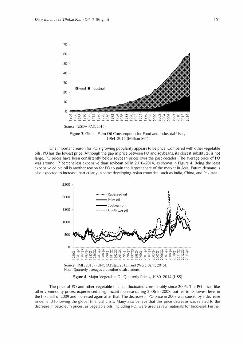
Palm oil is predominantly served as edible oil. However, it can also be used for industrial purposes.

Figure 3 shows the global consumption of PO for food and industrial uses. The figure shows that total

consumption of PO increased more than five-fold between 1990 and 2015, from 11 million MT in 1990 to 61

million MT in 2015. However, the growth rate of industrial PO exceeded that for edible PO. During the same

period, PO used for non-food industry grew by more than 700 percent, from 1.9 million MT to 16.3 million MT,

while PO used for food increased by 400 percent, from 9 million MT to 45 million MT. In 1980, almost 100

percent of PO was served as food. In 2015, this had decreased to 73 percent.

Though this figure does not mention in detail what the industrial purposes are, many believe that this

is strongly correlated with the growing increase of the biodiesel industry, especially in European countries (Lam

et al., 2009, Lam et al., 2009, Murphy, 2009). According to Mitchel (2008), biodiesel was responsible for

approximately one-third of the increase in vegetable oil consumption in 2004♠2007. In the early 19th century

Europe, PO was predominantly used for soap, candles and heating (Henderson & Osborne, 2000). Nowadays,

according to Gerasimchuk and Koh (2013), biodiesel feedstock in Europe increased by 365 percent from 2006

to 2012, equivalent to an increase from 0.4 million MT to 1.9 million MT, and an increase of 40 percent for

electricity and heat generation from 0.4 million MT to 0.6 million MT. For comparison, the use of PO for other

purposes, mainly food, increased by 6 percent (Gerasimchuk and Koh, 2013). This is important, since Europe is

the largest producer of biodiesel (Tan et al., 2009, Zhou and Thomson, 2009). There is also a growing interest

in biodiesel production in Asian countries, especially PO-based biodiesel in Indonesia and Malaysia (Mekhilef,

Siga and Saidur, 2011, Santosa, 2008, Wirawan and Tambunan, 2006, Zhou and Thomson, 2009).


Source: (USDA-FAS, 2016).

Figure 3. Global Palm Oil Consumption for Food and Industrial Uses,

1964♠2015 (Million MT)

One important reason for PO☂s growing popularity appears to be price. Compared with other vegetable

oils, PO has the lowest price. Although the gap in price between PO and soybeans, its closest substitute, is not

large, PO prices have been consistently below soybean prices over the past decades. The average price of PO

was around 17 percent less expensive than soybean oil in 2010♠2014, as shown in Figure 4. Being the least

expensive edible oil is another reason for PO to gain the largest share of the market in Asia. Future demand is

also expected to increase, particularly in some developing Asian countries, such as India, China, and Pakistan.

Source: (IMF, 2015), (UNCTADstat, 2015), and (Word Bank, 2015).Note: Quarterly averages are author☂s calculations.

Figure 4. Major Vegetable Oil Quarterly Prices, 1980♠2014 (US$)

The price of PO and other vegetable oils has fluctuated considerably since 2005. The PO price, like

other commodity prices, experienced a significant increase during 2006 to 2008, but fell to its lowest level in

the first half of 2009 and increased again after that. The decrease in PO price in 2008 was caused by a decrease

in demand following the global financial crisis. Many also believe that this price decrease was related to the

decrease in petroleum prices, as vegetable oils, including PO, were used as raw materials for biodiesel. Further

0

10

20

30

40

50

60

70

19

64

19

66

19

68

19

70

19

72

19

74

19

76

19

78

19

80

19

82

19

84

19

86

19

88

19

90

19

92

19

94

19

96

19

98

20

00

20

02

20

04

20

06

20

08

20

10

20

12

20

14

Food Industrial

0

500

1000

1500

2000

2500

1980Q

1

1981Q

2

1982Q

3

1983Q

4

1985Q

1

1986Q

2

1987Q

3

1988Q

4

1990Q

1

1991Q

2

1992Q

3

1993Q

4

1995Q

1

1996Q

2

1997Q

3

1998Q

4

2000Q

1

2001Q

2

2002Q

3

2003Q

4

2005Q

1

2006Q

2

2007Q

3

2008Q

4

2010Q

1

2011Q

2

2012Q

3

2013Q

4

Rapeseed oil

Palm oil

Soybean oil

Sunflower oil


research concerning vegetable oils and energy markets can be found in Abdel and Arshad (2008), Peri and Baldi

(2010), Priyati and Tyers (2016), Sanders, Balagtas and Gruere (2014), and Yu et al. (2006).

The main possible factors explaining why PO prices are very competitive are lower production costs

and higher yields compared with other major vegetable oils. Unlike other oils, such as soybean, rapeseed or

sunflower oil, which are annual crops, oil palms are a perennial crop with year-round harvesting. Palm oil incurs

less production costs and less labour costs, since oil palm plantations are mostly found in countries like Indonesia

and Malaysia where lower wages are paid to workers (Murphy, 2009a). According to Carter et al. (2007), the

average production cost of PO in 2004♠2005 was slightly above US$200, compared with more than US$300

for sunflower and soybean oils and more than US$500 for rapeseed oil.

Yield-wise, PO also appeared to have the highest productivity per ha compared with other vegetable

oils. With an average yield of nearly 4 MT/hectare/year excluding palm kernel oil (PKO) which is also derived

from oil palm fruits, the PO was more productive than other oils, which had a productivity of less than 0.5

MT/hectare/year (Johnston et al., 2009 and Murphy, 2009a).

Methods

The gravity model

Palm oil is generally shipped in bulk, because the unit price is relatively low. Asia is the most important market

for Indonesian PO. In 2010, almost 70 percent of Indonesian PO was exported to Asian countries, with the

largest and second largest being India (32 percent) and China (13 percent). In this case, proximity might be an

important factor to determine the flow of PO trades. The fact that Indonesia and Malaysia are close to these

large and rapidly growing markets may help explain the rapid growth in their PO exports. This is an interesting

hypothesis that will form the basis of our gravity model.

The role of distance in international trade is commonly investigated by the gravity model. The

traditional gravity model was introduced by Tinbergen (1962). He proposed that trade between two countries

is determined in part by their sizes and distance. Size determines the volume of demand and distance explains

the transportation cost.

The gravity model has been empirically successful in explaining international trade flows. The

theoretical foundations of the gravity model have been discussed by Anderson (1979), Bergstrand (1985),

Bergstrand (1989), and Deardorff (1998). This model is mainly employed for general trade, with an emphasis

on trade agreements or free trade zones. Only a few specific commodities have been investigated using the

gravity model. A few examples of the gravity model being employed with a specific emphasis in agricultural

good trades are Lambert and Grant (2008), Hatab, Romstad and Huo (2010), Olper and Raimondi (2008), and

Sarker and Jayasinghe (2007).

In its simplest form, the gravity equation can be written as:

(1)

Where Mjit determines imports of country j to country i in year t, and determine GDP of country i and j,

and is the distance between i and j. In our gravity model specification, we include several additional

variables, such as per capita income of both country i and country j (PY), the relative price of PO over soybean

oil (RP), importer-specific importer dummy variable (D), and interaction dummies for their incomes (DY). Taking

the logarithms, the gravity model specification can be written as:

(2)

Where, is the GDP of exporter countries and is the GDP of importer countries. Both exporters☂ and

importers☂ GDPs are used to represent supply and demand factors, respectively (Egger & Pfaffermayr, 2003).

Therefore, we expect both and to have positive signs. The distance between exporter and importer

countries is represented by . Distance is used as a proxy for transport cost to export goods from one

country to another. The greater the distance between two countries, the higher the transport cost, which also

means the trade flow between those two countries will be lesser. So, the expected sign of is negative.

We also add per capita income growth of both exporter and importer countries and the relative price

of PO over its closest substitute, soybean oil. Where, is per capita GDP of exporter countries, and is

per capita GDP of importer countries. The positive and statistically significant coefficient of exporter per capita

31 20 (1)jit it jt ijM Y Y Dist

0 1 2 3 4 4 5

6 7

ln ln ln ln ln ln + ln (2)

tjit it jt ij it jt

jt jt t

M Y Y Dist PY PY RPD D Y


income ( ) suggests that the good is capital intensive, otherwise it is labour-intensive. For importer countries,

positive and statistically significant per capita GDP ( ) suggests that the good is luxurious; otherwise it is a

necessity (Bergstrand, 1989).

The first five variables are standard properties in the gravity model. To capture the substitution between

PO and soybean oil, we have added relative price of PO over soybean oil ( ) . We assume people will

shift from palm oil to soybean oil when the price of palm oil increases, and vice versa. Therefore, we expect a

negative sign of .

We also introduce the importer-specific effect; therefore, we add dummy variables for India and China

as the countries of interest ( ). Additionally, we also include the interaction dummies of their incomes, which

equals the multiplication of importer dummy and the log of income ( ln ) . Since we only have two

dummies (China and India), there will be only two interaction dummies ( ln ) and ( ln ),as they are the two most important importers of PO from Indonesia and Malaysia, which imported around 33

percent of global PO in 2010.

Data

Throughout this paper, we will use Standard International Trade Classification (SITC) revision-3. Under this

classification, PO is coded as 4222, while its disaggregated products, crude PO (CPO) and refined PO (RPO) are

under 42221 and 42229 classifications, respectively. Palm kernel oil (PKO/4224), another product derived from

oil palm fruit, is beyond the scope of this paper, since it is sold in different markets and used in different

industries.

The model is estimated using annual import data reported by almost all countries (some are excluded

because of the lack of data) importing PO that originated in Indonesia and Malaysia. The model only covers

imports from Indonesia and Malaysia because they represent around 90 percent of global PO trade. The analysis

will be carried out using SITC classification: 4222 for PO, 42221 for CPO, and 42229 for RPO. The imported

country lists are in Appendix A1.

Table 2. Summary of Variables and Data Sources

mjit

: import of country j from country j measured in US$ (2000) constant price, data for export and importare obtained from UN-COMTRADE (http://wits.worldbank.org/wits/) and deflated by US importprice indices obtained from US Bureau of Labour Statistics database

(http://www.bls.gov/data/#prices).y

it: constant GDP of country i, data obtained from World Development Indicator (WDI), The World Bank

(http://data.worldbank.org/data-catalog/world-development-indicators)y

jt: constant GDP of country j, data obtained from WDI

pyit

: constant GDP per capita of country i, data obtained from WDIpy

jt: constant GDP per capita of country j, data obtained from WDI

distij

: distance between i dan j, obtained from Mayer and Zignago (2011) available at French Institute forResearch on International Economy (CEPII) database,(http://www.cepii.fr/anglaisgraph/bdd/distances.htm)

rp(PO/SBO)t

: relative price of palm oil over soybean oil to capture the substitution effect between palm oil andsoybean oil, data obtained from the World Bank commodity markets (pink sheet)(http://econ.worldbank.org/).

dIND

: dummy for India, 1=India, otherwise=0d

CHN: dummy for China, 1=China, otherwise=0

dINDy

jt: Interaction dummy for India, d

INDy

jt= d

IND* y

jt

dCHNy

jt: Interaction dummy for China, d

CHNy

jt= d

CHN* y

jt

i : exporter countries (Indonesia and Malaysia)j : importer countries (all countries#)

Note: # some countries are omitted because of data limitations.

We focus on the period between 1999 and 2011. We have chosen the starting year of 1999 because in

1998 the Indonesian government banned PO exports for several months as a result of the depreciation of the

Rupiah following the Asian financial crisis in 1997. We use PO import data of country j from both Indonesia

and Malaysia obtained from the United Nations Commodity Trade Statistics Database (UN-COMTRADE). Since

the import data is in current value, we deflate it by the US import indices taken from the US Bureau of Labour


Statistics. The GDP and per capita GDP are in constant 2000 US dollars obtained from WDI, available from the

World Bank website. Other variables and data sources are summarised in Table 2.

Results and Discussions

We estimate the gravity model on PO trade using panel data of two exporter countries (Indonesia and Malaysia)

and 157 importer countries, over the period of 1999♠2011. We include time fixed effects in model 2, model 3

and model 4 as in Egger and Pfaffermayr (2003) and Matyas (1997). Importer effect comes as importer-specific

effects for India and China. However, since there are only two exporter countries included in this analysis, we

exclude exporter fixed effects. The analysis will be carried out using ordinary least squares (OLS) and Poisson

pseudo-maximum-likelihood (PPML). The first is a standard method used in the majority of gravity models in

the relevant literature, and the latter is an alternative proposed by Silva and Tenreyro (2006). They argue that

PPML estimation can be used to deal with zero trade problems and is found to be consistent even in the presence

of heteroskedasticity (Silva & Tenreyro, 2006).

Table 3. Gravity Equation Estimates: Palm Oil (SITC 4222)

Variable OLS PPML

Model Model

1 2# 3# 4# 1 2# 3# 4#

LnGDP:

exporter (Yit) 1.42***

(0.21)"0.42(2.33)

"0.40(2.33)

"0.41(2.33)

1.97***

(0.22)3.03(2.09)

3.01(1.99)

3.00(2.01)

importer (Yjt) 1.14***

(0.03)1.14***

(0.03)1.12***

(0.03)1.12***

(0.03)0.93***

(0.02)0.93***

(0.02)0.78***

(0.04)0.79***

(0.04)

LnGDP per capita:

exporter (PYit) 0.87***

(0.09)0.19(0.86)

0.20(0.86)

0.20(0.86)

0.79***

(0.09)1.19(0.77)

1.20(0.74)

1.19(0.75)

importer (PYjt) "0.80***

(0.04)"0.80***

(0.04)"0.78***

(0.04)"0.78***

(0.04)"0.67***

(0.04)"0.67***

(0.04)"0.49***

(0.06)"0.49***

(0.06)Ln distance (Distij) "0.77***

(0.10)"0.78***

(0.10)"0.76***

(0.10)"0.76***

(0.10)"0.62***

(0.07)"0.62***

(0.07)"0.61***

(0.07)"0.61***

(0.07)Ln relative price

(RP(PO/SBO)t)"0.89(0.09)

0 0 0 "0.83(0.68)

1.63(7.55)

1.60(7.22)

1.67(7.21)

Dummy:

India (DIND) " " 0.75***

(0.27)11.38(9.27)

" " 0.78***

(0.25)3.99(7.99)

China (DCHN) " " 0.48***

(0.19)"9.13***

(2.36)

" " 0.62***

(0.18)"3.58(3.28)

Interaction dummy:

DIND*ln YIND " " " "0.79(0.70)

" " " "0.24(0.60)

DCHN*lnYCHN " " " 0.66***

(0.16)

" " " 20.29(0.23)

constant "14.72***

(3.23)11.68(33.83)

11.36(33.83)

11.38(33.85)

"19.38***

(3.12)"35.17(31.05)

"34.95(29.59)

"34.71(29.88)

N 2537 2537 2537 2537 3668 3668 3668 3668R2 0.42 0.43 0.43 0.43 0.64 0.65 0.67 0.66F-statistic 317.21 114.00 411.93 682.89RMSE 2.30 2.30 2.29 2.30Log pseudo-likelihood "8.91e+

07"8.79e+07

"8.58e+07

"8.56e+07

Note: dependent variables are import values in natural logarithms (ln) for OLS and in levels for PPML. Figures inparentheses are robust standard errors.#includes time fixed effect.Individual time fixed effect is not reported.*** indicates that a coefficient is significant at the 1% level and **significant at the 5% level.

Table 3 presents the OLS panel and the alternative results from PPML for PO. Overall, the results of

OLS and PPML are consistent with the general results in the gravity literature. That is, on average all the

significant income coefficients are close to unity. The distance coefficients are between "0.78 and "0.61. In

both tables, the first column (model 1) shows the model without time fixed effects; while all other three columns

(models 2, 3 and 4) show the results with time fixed effects. The R2 ranges between 0.42 and 0.43 for OLS and

higher for PPML between 0.64 and 0.67. This means that PPML generally performs better than OLS. Also in


line with Silva and Tenreyro (2006), we found that the coefficient of most variables were lower in PPML

compared with OLS.

The main result is that importers☂ GDP and GDP per capita variables are estimated to be strongly

significant (p<0.01), and this is consistent across models. The importer☂s GDP coefficients for PO reported in

Table 3 all have positive signs and are all close to unity. For PPML, importers☂ GDP coefficients are slightly

smaller than OLS results, ranging from 0.78 to 0.93.

The elasticity reported for GDP per capita of importer countries was found to be negative and significant

for PO both from OLS and PPML results. These results are also in line with Sarker and Jayasinghe (2007) who

found that importer☂s GDP per capita was negatively correlated for oilseeds and vegetables in the European market.

Our results suggest that PO imports will decrease by between 0.78 percent and 0.8 percent with every 1 percent

per capita income increase when using OLS, and 0.49 percent and 0.67 percent when using PPML.

Our findings also prove that the bilateral distances between trading partners are negatively correlated

in PO trade. The elasticities of distances are around "0.8 for OLS and around "0.6 for PPML. As mentioned

earlier, PO imports used in this analysis come from Indonesia and Malaysia only, where almost 90 percent of

global PO originates. For both countries, China and India constitute the most important importers of PO. In fact,

in 2011, both China and India absorbed around 40 percent of total PO from Indonesia and Malaysia. The growth

of both countries could be an important determinant of PO demand.

Table 4. Gravity Equation Estimates: Crude Palm Oil (SITC 42221)

Variable OLS PPML

Model Model

1 2# 3# 4# 1 2# 3# 4#

LnGDP:


(0.36)3.13(3.93)

3.12(3.90)

2.94(3.91)

2.92***

(0.44)5.10(3.75)

5.09*

(2.82)5.08*

(2.81)


(0.06)0.88***

(0.06)0.88***

(0.07)0.88***

(0.07)0.82***

(0.05)0.82***

(0.05)0.67***

(0.04)0.67***

(0.05)LnGDP per capita:

exporter (PYit) "0.09(0.15)

0.39(1.45)

0.39(1.44)

0.32(1.44)

0.47***

(0.15)1.30(1.39)

1.32(1.07)

1.31(1.06)


(0.07)"0.74***

(0.07)"0.72***

(0.08)"0.72***

(0.08)"0.68***

(0.09)"0.68***

(0.09)"0.40***

(0.08)"0.40***


(0.15)

"0.56***

(0.15)

"0.55***

(0.16)

"0.55***

(0.16)

"0.79***

(0.12)

"0.79***

(0.12)

"0.78***

(0.11)

"0.78***


(RP(PO/SBO)t)0.26(0.97)

0 0 0 "1.44(1.19)

6.46(14.75)

6.52(9.38)

6.89(9.25)

Dummy:

India (DIND) " 1.80**

(0.39)"21.41**

(9.95)

" " 1.68***

(0.25)"4.62(6.09)

China (DCHN) " "1.61***

(0.52)"45.19***

(12.55)

" " "1.09***

(0.30)"9.15(9.34)

Interaction dummy:

DIND*ln YIND " " 1.73**

(0.735)

" " 0.46(0.45)

DCHN*lnYCHN " " 3.01***

(0.86)

" " 0.55(0.64)

Constant "12.53**

(5.38)"31.53(56.77)

"31.52(56.43)

"28.78(56.49)

"26.59***

(6.16)"58.83(55.85)

"59.54(42.09)

"59.34(41.88)

N 1398 1398 1398 1398 3668 3668 3668 3668R2 0.24 0.24 0.25 0.25 0.33 0.34 0.74 0.74F-statistic 58.35 21.51 59.23 130.93 "RMSE 2.82 2.83 2.81 2.81Log pseudo-likelihood "6.88e+07 6.81e+07 "5.74e+07 "5.73e+07

Note: dependent variables are import values in natural logarithms (ln) for OLS and in levels for PPML.Figures in parentheses are robust standard errors.#includes time fixed effect.Individual time fixed effect is not reported.*** indicates that a coefficient is significant at the 1% level and **significant at the 5% level.

To capture the importance of China and India, we included country specific effects for China and India

as dummy variables in model 3 and model 4. In model 3, we found that both dummies for India and China are

significant. The coefficients of Indian dummies for PO are 0.75 for OLS and 0.78 for PPML; for China, the


dummy coefficients are 0.48 for OLS and 0.62 for PPML. Overall, India has a bigger impact on PO trade than

China. The OLS results suggest that India imports 2.12 (exp(0.75)) times more PO than non-India and non-China

countries, and China imports 1.57 (exp(0.48)) times more PO than non-China and non-India countries.

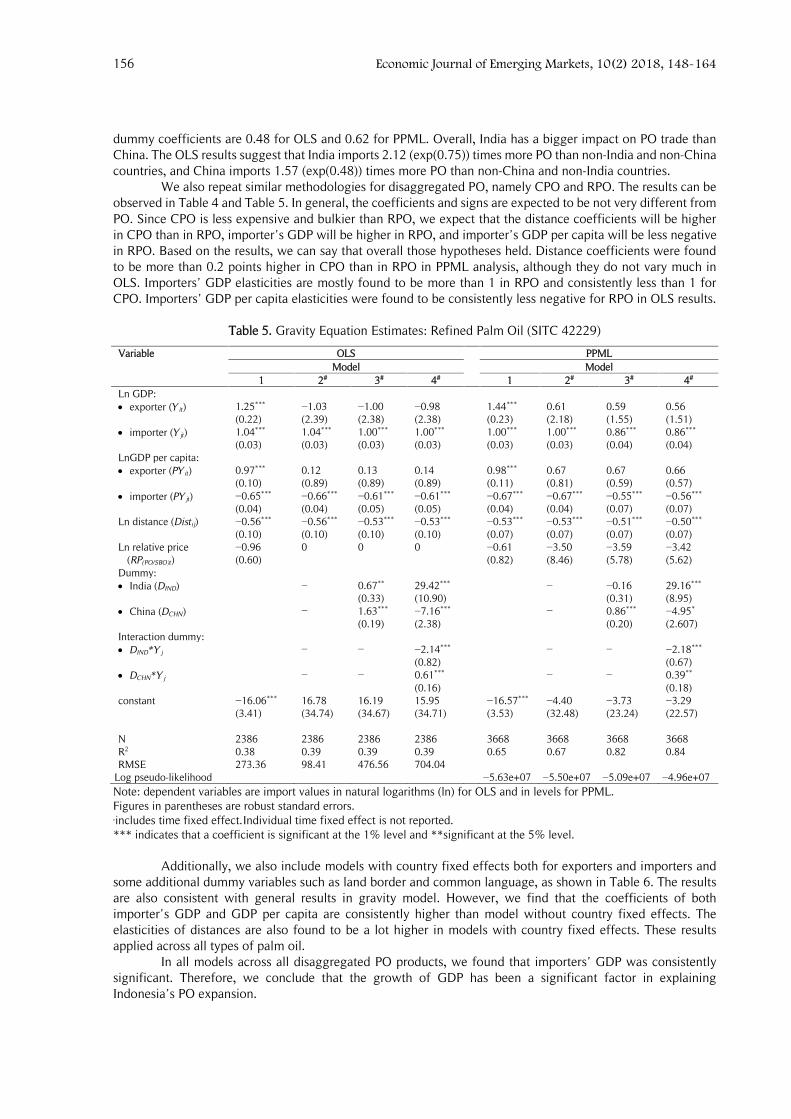
We also repeat similar methodologies for disaggregated PO, namely CPO and RPO. The results can be

observed in Table 4 and Table 5. In general, the coefficients and signs are expected to be not very different from

PO. Since CPO is less expensive and bulkier than RPO, we expect that the distance coefficients will be higher

in CPO than in RPO, importer☂s GDP will be higher in RPO, and importer☂s GDP per capita will be less negative

in RPO. Based on the results, we can say that overall those hypotheses held. Distance coefficients were found

to be more than 0.2 points higher in CPO than in RPO in PPML analysis, although they do not vary much in

OLS. Importers☂ GDP elasticities are mostly found to be more than 1 in RPO and consistently less than 1 for

CPO. Importers☂ GDP per capita elasticities were found to be consistently less negative for RPO in OLS results.

Table 5. Gravity Equation Estimates: Refined Palm Oil (SITC 42229)

Variable OLS PPML

Model Model

1 2# 3# 4# 1 2# 3# 4#

Ln GDP:


(0.22)"1.03(2.39)

"1.00(2.38)

"0.98(2.38)

1.44***

(0.23)0.61(2.18)

0.59(1.55)

0.56(1.51)


(0.03)1.04***

(0.03)1.00***

(0.03)1.00***

(0.03)1.00***

(0.03)1.00***

(0.03)0.86***

(0.04)0.86***

(0.04)LnGDP per capita:

exporter (PYit) 0.97***

(0.10)0.12(0.89)

0.13(0.89)

0.14(0.89)

0.98***

(0.11)0.67(0.81)

0.67(0.59)

0.66(0.57)


(0.04)"0.66***

(0.04)"0.61***

(0.05)"0.61***

(0.05)"0.67***

(0.04)"0.67***

(0.04)"0.55***

(0.07)"0.56***


(0.10)"0.56***

(0.10)"0.53***

(0.10)"0.53***

(0.10)"0.53***

(0.07)"0.53***

(0.07)"0.51***

(0.07)"0.50***


(RP(PO/SBO)t)"0.96(0.60)

0 0 0 "0.61(0.82)

"3.50(8.46)

"3.59(5.78)

"3.42(5.62)

Dummy:

India (DIND) " 0.67**

(0.33)29.42***

(10.90)

" "0.16(0.31)

29.16***

(8.95)

China (DCHN) " 1.63***

(0.19)"7.16***

(2.38)

" 0.86***

(0.20)"4.95*

(2.607)Interaction dummy:

DIND*Yj " " "2.14***

(0.82)

" " "2.18***

(0.67)

DCHN*Yj " " 0.61***

(0.16)

" " 0.39**

(0.18)constant "16.06***

(3.41)16.78(34.74)

16.19(34.67)

15.95(34.71)

"16.57***

(3.53)"4.40(32.48)

"3.73(23.24)

"3.29(22.57)

N 2386 2386 2386 2386 3668 3668 3668 3668R2 0.38 0.39 0.39 0.39 0.65 0.67 0.82 0.84RMSE 273.36 98.41 476.56 704.04

Log pseudo-likelihood "5.63e+07 "5.50e+07 "5.09e+07 "4.96e+07

Note: dependent variables are import values in natural logarithms (ln) for OLS and in levels for PPML.Figures in parentheses are robust standard errors.#includes time fixed effect.Individual time fixed effect is not reported.*** indicates that a coefficient is significant at the 1% level and **significant at the 5% level.

Additionally, we also include models with country fixed effects both for exporters and importers and

some additional dummy variables such as land border and common language, as shown in Table 6. The results

are also consistent with general results in gravity model. However, we find that the coefficients of both

importer☂s GDP and GDP per capita are consistently higher than model without country fixed effects. The

elasticities of distances are also found to be a lot higher in models with country fixed effects. These results

applied across all types of palm oil.

In all models across all disaggregated PO products, we found that importers☂ GDP was consistently

significant. Therefore, we conclude that the growth of GDP has been a significant factor in explaining

Indonesia☂s PO expansion.


Table 6. Gravity Equation Estimates: OLS Results with Country Fixed Effects

and Additional Dummies

Variable PO CPO RPO

Ln GDP:

exporter (Yit) 0.71**

(0.05)-1.76(0.22)

1.00*(0.08)

-3.57(0.14)

1.10***(0.00)

0.64(0.7)


(0.00)4.43***(0.00)

1.81***(0.00)

1.53(0.27)

2.13***(0.00)

3.64***(0.00)

LnGDP per capita:

exporter (PYit) 3.12

(0.13)6.40*(0.06)

0.23(0.92)

importer (PYjt) -2.03***

(0.00)0.46(0.77)

-1.75**(0.01)

Ln(dist) -1.57**(0.04)

-1.59**(0.04)

-2.01(0.14)

-1.96(0.15)

-2.11***(0.01)

-2.11***(0.01)

Ln relative price

(RP(PO/SBO)t

)

-1.11**

(0.02)

-1.28***

(0.01)

- -1.89**

(0.15)

- -0.93*

(0.08)Dummy:

border 1.74**(0.02)

1.77**(0.0.02)

-0.61(0.76)

-0.41(0.84)

2.06***(0.00)

2.07***(0.00)

common language 0.83**(0.04)

0.82**(0.04)

1.07(0.16)

1.00(0.18)

0.52(0.15)

0.53(0.14)

Constant -59.81***(0.00)

-57.11***(0.01)

-37.97***(0.01)

18.47(0.63)

-46.51***(0.00)

-60.51***(0.01)

Exporter fixed effect yes yes yes yes yes YesImporter fixed effect yes yes yes yes yes yesn 2537 2537 1398 1398 2386 2386R2 0.73 0.73 0.69 0.70 0.69 0.69

Note: dependent variables are import values in natural logarithms (ln).Figures in parentheses are probabilities.*** indicates that a coefficient is significant at the 1% level, **significant at the 5% level and *significant at 10% level.

Mostly backed by descriptive data, many papers mention the importance of India and China in

determining global PO demand, such as Corley (2009) and Koh and Wilcove (2007). This comes from the fact

that China and India alone are responsible for 40 percent of PO imports originating in Indonesia and Malaysia.

Given the preceding results, a relevant question is whether the growth of Indonesia☂s trading partners can

explain the growth in PO export demand. In particular, there has been rapid growth in China and India, which

are the two of Indonesia☂s largest trading partners. To what extent does the growth of income of Indonesia☂s

trading partners explain the boom in Indonesia☂s PO export demand? The estimated model 4 from PPML analysis

for PO (Table 3) is used for simulating PO imports from Indonesia for the period 2000♠201. We only include

the significant coefficients for the simulations. The importer☂s GDP coefficient in this model is 0.79, meaning

that a 1 percent increase in importer☂s GDP may lead to 0.79 percent of PO import from Indonesia.

For simplicity, we selected Indonesia☂s top 10 PO importers only. The selection is based on import data

from 2011. Total imports from these countries accounted for 73 percent of total PO exports from Indonesia.

India had the largest share, with nearly 40 percent, followed by China, with almost 20 percent. The total

Indonesian PO imported by the top 10 countries can be plotted in Figure 5. We use the estimated coefficients

for importer GDP (GDPj) and importer☂s GDP per capita (PGDPj) to estimate the share of PO trade for each top

10 country.

The simulated shares of PO imports from Indonesia to the top 10 countries based on importer GDP

(GDPj) and importer☂s per capita GDP (PGDPj) for the period 2000♠2011 are reported in Figures 6 (all top 10),

Figure 7 (China), and Figure 8 (India). More complete simulation results are reported in Appendix A2.


Source: UN-COMTRADE (WITS, 2015).

Figure 5. Indonesia☂s Palm Oil Exports, 1999♠2011 (Million US$)

Figure 6. Palm Oil Real Import and Import Simulation for the Top 10 Countries

(Million US$)

Overall, we find that GDPj and the combination of GDPj and PGDPj explain very little of the rapid

growth in PO export demand from Indonesia. For instance, over the sample period, China☂s GDP grew by 131

percent, while the growth of China☂s PO imports from Indonesia was more than 800 percent. For India, the

growth of GDP was 95 percent, while the actual growth of PO imports from Indonesia was more than 1000

percent.

0

2000

4000

6000

8000

10000

12000

1999 2000 2001 2002 2003 2004 2005 2006 2007 2008 2009 2010 2011

TotalTop 10

0

1000

2000

3000

4000

5000

6000

7000

8000

9000

1999 2000 2001 2002 2003 2004 2005 2006 2007 2008 2009 2010 2011

Real M (T-10) SimGDPj SimGDPj+PGDPj


Figure 7. Palm Oil Real Import and Import Simulation for China (Million US$).

Figure 8. Palm Oil Real Import and Import Simulation for India (Million US$).

Figure 6 shows that, consistent with results for China and India, the actual PO imports from Indonesia

to all countries are far more than the simulated PO imports explained by importer☂s GDP and importer per capita

GDP. For example, the actual PO import to the top 10 countries was US$8.5 billion compared with only US$1.8

billion as projected by the growth in GDP (see Appendix A2).

These results suggest that income growth alone cannot be used to explain the boom in PO export

demand. There are possibly other variables that explain the vast increase in global PO demand, including

changing preferences, diversification in end uses and import tariff reduction, but those variables are not included

in this research.

Conclusion

Global vegetable oil demand has increased very rapidly in the last decade, with PO now being the most produced

vegetable oil, displacing soybean oil in 2007. Indonesia and Malaysia are the largest producers and exporters of

PO, capturing a combined market share of around 90% in 2014.

0

200

400

600

800

1000

1200

1400

1600

1800

1999 2000 2001 2002 2003 2004 2005 2006 2007 2008 2009 2010 2011

Real M (CHN) SimGDPj SimGDPj+PGDPj

0

500

1000

1500

2000

2500

3000

3500

4000

1999 2000 2001 2002 2003 2004 2005 2006 2007 2008 2009 2010 2011

Real M (IND) SimGDPj SimGDPj+PGDPj


In this paper, we employ gravity equations to observe the trade in palm oil market with only Indonesia

and Malaysia as exporters and all other countries as their importers. The gravity model is widely used to

investigate the role of distance and economic growth in international trade flows.

The results suggest that PO trade follows the general results in gravity literature. We find that importer

GDP and importer per capita GDP variables are consistently significant in all models in both OLS and PPML

used in this study. Our findings also prove that the bilateral distances between trading partners are negatively

correlated in PO trades. However, we are unable to confirm the importance of relative price between palm oil

and soybean oil in determining palm oil trade flows.

Given the large growth in China and India☂s GDP and their proximity to Indonesia and Malaysia, we

also examine the impact of China and India in the model. We find that both dummies for China and India are

positively correlated.

Furthermore, we do a simulation using the samples of top ten imported countries of Indonesia☂s palm

oil. We, particularly, observe how the economic growth of importer countries affect the flow of palm oil trade.

The simulation result for top ten Indonesia☂s trading partners suggest that the simulated palm oil trades

explained by importer GDPs account for only 15 percent in average when compared to the actual trade flows.

This result is also applied for China and India which both GDPs explain only 25 percent and 17 percent of their

actual palm oil imports. There are possibly other variables that explain the vast increase in global PO demand,

including changing preferences, diversification in end uses and import tariff reduction, but those variables are

not included in this research.

References

Abdel, H., & Fatimah Mohamed Arshad. (2008). The impact of petroleum prices on vegetable oils prices:

Evidence from cointegration tests. International Borneo Business ▁, 2008(January 2000), 31♠40.

Anderson, J. E. (1979). A theoretical foundation for the gravity equation. The American Economic Review,

69(1), 106♠116. https://doi.org/10.2307/1802501

Bergstrand, J. H. (1985). The gravity equation in international trade: Some microeconomic foundations and

empirical evidence. The Review of Economics and Statistics, 67(3), 474.

https://doi.org/10.2307/1925976

Bergstrand, J. H. (1989). The generalized gravity equation, monopolistic competition, and the factor-

proportions theory in international trade. The Review of Economics and Statistics, 71(1), 143.

https://doi.org/10.2307/1928061

Carter, C., Finley, W., Fry, J., Jackson, D., & Willis, L. (2007). Palm oil markets and future supply. European

Journal of Lipid Science and Technology, 109(4), 307♠314. https://doi.org/10.1002/ejlt.200600256

Corley, R. H. V. (2009). How much palm oil do we need? Environmental Science and Policy, 12(2), 134♠139.

https://doi.org/10.1016/j.envsci.2008.10.011

Deardorff, A. V. (1998). Chapter title: Determinants of bilateral trade: does gravity work in a neoclassic

world? Determinants of bilateral trade: Does gravity work in a neoclassical world?, ISBN, 0♠226.

Egger, P., & Pfaffermayr, M. (2003). The proper panel econometric specification of the gravity equation: A

three-way model with bilateral interaction effects. Empirical Economics, 28(3), 571♠580.

https://doi.org/10.1007/s001810200146

FAOstat. (2015). Production. Retrieved from http://www.fao.org/faostat/

Gerasimchuk, I., & Yam Koh, P. (2013). The EU biofuel policy and palm oil: Cutting subsidies or cutting

rainforest? The International Institute for Sustainable Development, (September), 20.

Hatab, A. A., Romstad, E., & Huo, X. (2010). Determinants of Egyptian agricultural exports: A gravity model

approach. Modern Economy, 01(03), 134♠143. https://doi.org/10.4236/me.2010.13015

Henderson, J., & Osborne, D. J. (2000). The oil palm in all our lives: How this came about. Endeavour, 24(2),

63♠68. https://doi.org/10.1016/S0160-9327(00)01293-X

IMF. (2015). IMF primary commodity prices. Retrieved from

https://www.imf.org/external/np/res/commod/index.aspx


Johnston, M., Foley, J. A., Holloway, T., Kucharik, C., & Monfreda, C. (2009). Resetting global expectations

from agricultural biofuels. Environmental Research Letters, 4(1), 014004.

https://doi.org/10.1088/1748-9326/4/1/014004

Koh, L. P., & Wilcove, D. S. (2007). Cashing in palm oil for conservation. Nature, 448(7157), 993♠994.

https://doi.org/10.1038/448993a

Koh, L. P., & Wilcove, D. S. (2008). Is oil palm agriculture really destroying tropical biodiversity?

Conservation Letters, 1(2), 60♠64. https://doi.org/10.1111/j.1755-263X.2008.00011.x

Lam, M. K., Tan, K. T., Lee, K. T., & Mohamed, A. R. (2009). Malaysian palm oil: Surviving the food versus

fuel dispute for a sustainable future. Renewable and Sustainable Energy Reviews, 13(6♠7), 1456♠

1464. https://doi.org/10.1016/j.rser.2008.09.009

Lambert, D. M., & Grant, J. H. (2008). Do regional trade agreements increase members☂ agricultural trade?

American Journal of Agricultural Economics, 90(3), 765♠782. https://doi.org/10.1111/j.1467-

8276.2008.01134.x

Matyas, L. (1997). Proper econometric specification of the gravity model. The World Economy, 20(3), 363♠

368. https://doi.org/10.1111/1467-9701.00074

Mekhilef, S., Siga, S., & Saidur, R. (2011). A review on palm oil biodiesel as a source of renewable fuel.

Renewable and Sustainable Energy Reviews, 15(4), 1937♠1949.

https://doi.org/10.1016/j.rser.2010.12.012

Mitchel, D. (2008). A note on rising food prices. The World Bank. https://doi.org/10.1596/1813-9450-4682

Murphy, D. J. (2009a). Global oil yields: Have we got it seriously wrong? Inform, 20, 499♠500.

https://doi.org/10.1088/1748-9326/4/1/014004.

Murphy, D. J. (2009b). Oil palm: Future prospects for yield and quality improvements. Lipid Technology,

21(11♠12), 257♠260. https://doi.org/10.1002/lite.200900067

Olper, A., & Raimondi, V. (2008). Agricultural market integration in the OECD: A gravity-border effect

approach. Food Policy, 33(2), 165♠175. https://doi.org/10.1016/j.foodpol.2007.06.003

Peri, M., & Baldi, L. (2010). Vegetable oil market and biofuel policy: An asymmetric cointegration approach.

Energy Economics, 32(3), 687♠693. https://doi.org/10.1016/j.eneco.2009.09.004

Priyati, R. Y., & Tyers, R. (2016). Economics price relationships in vegetable oil and energy markets price

relationships in vegetable oil and energy markets. Annual Australiasian Development Economics

Workshop.

Sanders, D. J., Balagtas, J. V., & Gruere, G. (2014). Revisiting the palm oil boom in South-East Asia: Fuel

versus food demand drivers. Applied Economics, 46(2), 127♠138.

https://doi.org/10.1080/00036846.2013.835479

Santosa, S. J. (2008). Palm oil boom in Indonesia: From plantation to downstream products and biodiesel.

Clean - Soil, Air, Water, 36(5♠6), 453♠465. https://doi.org/10.1002/clen.200800039

Sarker, R., & Jayasinghe, S. (2007). Regional trade agreements and trade in agri-food products: Evidence for

the European Union from gravity modeling using disaggregated data. Agricultural Economics, 37(1),

93♠104. https://doi.org/10.1111/j.1574-0862.2007.00227.x

Silva, J. M. C. S., & Tenreyro, S. (2006). The log of gravity. Review of Economics and Statistics, 88(4), 641♠

658. https://doi.org/10.1162/rest.88.4.641

Tan, K. T., Lee, K. T., Mohamed, A. R., & Bhatia, S. (2009). Palm oil: Addressing issues and towards

sustainable development. Renewable and Sustainable Energy Reviews, 13(2), 420♠427.

https://doi.org/10.1016/j.rser.2007.10.001

Tinbergen, J. (1962). Shaping the world economy: Suggestions for an international economic policy. Books

(Jan Tinbergen). Twentieth Century Fund, New York.

UNCTADstat. (2015). Free market commodity prices. United Nations Conference on Trade and Development.


Geneva.

USDA-FAS. (2016). Production, supply, and distribution.

Wirawan, S. S., & Tambunan, A. H. (2006). The current status and prospects of biodiesel development in

Indonesia: A review.

WITS. (2015). Trade data (UN Comtrade). Retrieved from https://comtrade.un.org/data/

Word Bank. (2015). Commodity markets. Retrieved from http://www.worldbank.org/en/research/commodity-

markets

Word Bank. (2016). World Bank Open Data. Retrieved from https://data.worldbank.org/

Yu, T.-H., Bessler, D. A., Fuller, S., & Bessler, D. (2006). Cointegration and causality analysis of world

vegetable oil and crude oil prices.

Zhou, A., & Thomson, E. (2009). The development of biofuels in Asia. Applied Energy, 86(SUPPL. 1), S11♠

S20. https://doi.org/10.1016/j.apenergy.2009.04.028


APPENDICES

Appendix A1. List of Indonesia and Malaysia Trading Partners on Palm Oil TradesAlbania Georgia NicaraguaUnited Arab Emirates Ghana Netherlands

Argentina Guinea NorwayArmenia Gambia* NepalAntigua and Barbuda** Greece New ZealandAustralia Guatemala OmanAustria Guyana** PakistanAzerbaijan Hong Kong, China PanamaBurundi Honduras** PeruBelgium Croatia PhilippinesBenin Hungary Papua New GuineaBurkina Faso Indonesia** PolandBangladesh India PortugalBulgaria Ireland Qatar**Bahrain** Iran, Islamic Rep. Romania

Bosnia and Herzegovina Iraq** Russian FederationBelarus Israel RwandaBrazil Italy Saudi ArabiaBarbados** Jamaica SudanBrunei Jordan SenegalBhutan Japan SerbiaBotswana** Kazakhstan SingaporeCentral African Republic Kenya Solomon IslandCanada Kyrgyz Republic El SalvadorSwitzerland Cambodia SurinameChile Kiribati** Slovak RepublicChina Korea, Rep. SloveniaCote d'Ivoire Kuwait Sweden

Cameroon Lebanon Seychelles**Congo, Rep. Libya** Syrian Arab RepublicColombia Saint Lucia** TogoComoros Sri Lanka ThailandCape Verde** Lithuania East Timor*Costa Rica** Luxembourg** Tonga*Cyprus Latvia Trinidad and TobagoCzech Republic Macao TunisiaGermany Morocco TurkeyDjibouti Moldova TanzaniaDominica** Madagascar UgandaDenmark Maldives** UkraineDominican Rep.** Mexico Uruguay

Algeria Macedonia, FYR United StatesEcuador Mali St. Vincent and the

Grenadines*Egypt, Arab Rep. Malta** VenezuelaEritrea** Mongolia VietnamSpain Mozambique VanuatuEstonia Mauritania SamoaEthiopia (excludesEritrea)

Mauritius Yemen

Finland Malawi South AfricaFiji Malaysia* ZambiaFrance Namibia ZimbabweGabon Niger

United Kingdom Nigeria

Note: *trade with Indonesia only. **trade with Malaysia only.


Appendix A2. Simulation Results (Million US$)Real data

CHN DEU EGY IND ITA MYS NLD PAK RUS TZA Total

2000 146.84 74.02 11.06 357.88 7.22 9.54 102.91 4.29 10.52 30.62 754.902001 102.39 84.75 10.16 381.86 13.77 19.13 110.61 26.59 25.33 42.66 817.252002 199.89 116.53 6.81 568.32 11.59 115.45 182.45 108.45 43.53 52.31 1405.332003 384.11 111.96 1.73 1069.20 25.84 143.77 189.75 101.76 51.30 66.05 2145.472004 535.29 156.63 44.21 1242.50 60.39 336.91 233.15 226.43 54.84 68.94 2959.292005 501.43 148.67 33.44 902.56 66.38 134.52 219.46 288.59 98.36 68.94 2462.342006 618.73 155.47 178.68 824.34 77.63 224.22 226.98 309.43 96.81 106.87 2819.152007 783.16 237.96 74.23 974.75 85.75 196.28 304.36 345.78 90.07 79.31 3171.662008 1437.37 406.57 388.47 1770.77 314.63 463.21 571.92 383.81 94.56 33.92 5865.252009 1290.31 293.04 211.83 2229.89 395.05 545.85 490.15 112.89 81.16 56.17 5706.342010 1430.67 373.11 161.18 2823.77 421.00 780.54 434.60 31.01 210.33 65.35 6731.57

2011 1643.66 262.79 323.69 3436.91 394.70 1237.86 518.50 152.96 333.96 159.72 8464.75

Simulation: GDPj

2000 185.17 57.54 7.31 316.50 22.43 74.05 123.86 4.86 8.58 2.72 803.022001 202.47 58.52 7.60 334.07 22.90 74.48 126.53 4.97 9.07 2.91 843.522002 223.22 58.52 7.80 348.73 23.02 78.99 126.64 5.15 9.55 3.14 884.762003 248.36 58.28 8.08 379.90 23.00 84.13 127.12 5.43 10.34 3.38 948.022004 276.62 59.04 8.45 413.45 23.45 90.55 130.30 5.88 11.17 3.68 1022.602005 311.86 59.49 8.88 456.68 23.70 95.97 133.29 6.39 11.97 3.99 1112.222006 356.55 61.96 9.56 504.32 24.28 102.28 138.37 6.83 13.07 4.29 1221.512007 413.72 64.23 10.32 560.00 24.74 109.73 144.46 7.27 14.33 4.63 1353.43

2008 458.45 65.01 11.16 584.46 24.42 115.66 147.38 7.40 15.17 5.02 1434.122009 505.94 61.29 11.74 638.65 22.92 113.54 141.56 7.70 13.85 5.36 1522.552010 565.23 63.83 12.42 707.35 23.38 122.73 144.24 8.05 14.52 5.79 1667.542011 624.42 65.97 12.67 761.88 23.50 129.81 146.14 8.27 15.22 6.20 1794.08

Simulation: GDPj+PGDPj

2000 195.67 58.85 7.51 322.00 23.06 77.67 126.94 4.93 9.24 2.77 828.642001 226.00 60.47 7.91 348.42 23.87 77.03 130.85 5.04 10.18 3.04 892.812002 264.72 60.40 8.15 370.09 24.02 83.62 130.39 5.27 11.15 3.39 961.212003 314.96 59.95 8.53 422.74 23.85 91.47 130.74 5.69 12.80 3.77 1074.492004 375.43 61.29 9.07 482.19 24.45 101.94 135.98 6.42 14.66 4.27 1215.70

2005 456.65 62.11 9.72 564.13 24.74 110.80 141.06 7.29 16.54 4.78 1397.832006 568.63 66.61 10.86 659.90 25.67 121.67 150.11 8.05 19.27 5.30 1636.082007 725.89 70.88 12.20 779.31 26.35 135.25 161.21 8.82 22.56 5.91 1948.392008 858.38 72.46 13.72 828.64 25.62 145.97 166.28 8.96 24.89 6.62 2151.542009 1008.19 65.69 14.76 952.63 22.90 139.70 154.66 9.45 21.32 7.23 2396.542010 1208.67 70.46 16.02 1120.74 23.61 157.43 159.03 10.07 23.09 8.04 2797.162011 1422.35 74.56 16.35 1257.73 23.71 171.00 161.98 10.38 25.01 8.83 3171.89

Determinants of Global Palm Oil Demand: A Gravity Approach

Documents

Transcript of Determinants of Global Palm Oil Demand: A Gravity Approach